quantifying benefits of signal timing maintenance and ...docs.trb.org/prp/15-1343.pdf ·...
TRANSCRIPT

Quantifying Benefits of Signal Timing Maintenance and
Optimization Using both Travel Time and Travel Time
Reliability Measures by
Howell Li
Purdue University
Steven M. Lavrenz
Purdue University
Christopher M. Day
Purdue University
Amanda Stevens
Indiana Department of Transportation
Corresponding author:
Darcy M. Bullock
Purdue University
550 Stadium Mall Drive
West Lafayette, IN 47906
Phone (765) 494-2226
Word Count: 4,558 words + 10 * 250 words/(figure-table) = 7,058 words
November 14, 2014
Li, Lavrenz, Day, Stevens, Sturdevant, Bullock 15-1343
2
ABSTRACT 1
Maintaining and optimizing signal timing directly contributes to an improved end-user driving 2
experience. With recent developments in crowd-sourced vehicle probe data, travel time 3
improvements associated with signal re-timings can be quantitatively assessed without costly 4
infrastructure. 5
This study compares the performance of three signal re-timing scenarios—1) pre-6
maintenance, 2) post- time-of-day and clock maintenance, and 3) post-progression optimization—7
for the weekday AM peak, mid-day, and PM peak time periods. The percentage of vehicles arriving 8
on green and vehicle travel time distributions were evaluated for each of the tasks in each period. 9
User benefits were then quantified using the travel time data with the mean-variance method to 10
determine the dollar savings for the tasks performed. Signal time-of-day plan maintenance and 11
clock synchronization accounted for some of the travel time benefits, but the savings were less 12
reliable than progression optimization, which improved both travel times and reliability. 13
14

Li, Lavrenz, Day, Stevens, Sturdevant, Bullock 15-1343
3
MOTIVATION 1
Quantifying signalized corridor travel time performance generally involves investment in data 2
collection infrastructure, equipment, and manpower. For decades, travel time assessment for a 3
signalized corridor was only possible with manual in-vehicle time keeping, instrumented probe 4
vehicles acting as singular data points to record the trajectory and control delay at every 5
intersection [1], or through the use of videography and manual counting. In 2008, Bluetooth re-6
identification emerged as a technology that could provide much larger and representative sample 7
sizes using data collection devices placed at strategically instrumented locations along an arterial 8
[2]. 9
10
There have been many performance measures developed in the last decade to assess arrival 11
characteristics, delay, and travel time through a signalized arterial using high-resolution signal 12
event data [3, 4, 5]. These data are digital logs of controller events, including phase and detector 13
activations, to one-tenth of a second time resolution. However, because these performance 14
measures are developed from the data on an intersection-by-intersection basis, such as arrival on 15
green (AOG) and volume-to-capacity ratio, they do not necessarily capture an individual driver’s 16
direct experience through multiple intersections [6]. More recently, crowd-sourced probe vehicle 17
data has enabled performance assessment of arterials without intrusive infrastructure. The data has 18
gained in both precision and robustness with the ever-growing ubiquity of smart phone adoption 19
[7]. The increased geographic and temporal resolution make crowd-sourced data a valuable 20
emerging resource for evaluating the effects of corridor maintenance and re-timing operations on 21
travel time. Consequently, opportunities have arisen to combine the crowd-sourced travel time 22
data with localized high-resolution signal event data to characterize user improvements using 23
volume-weighted methods [8]. 24
25
As many agencies struggle with shortfalls in funding, basic signal maintenance tasks such as clock 26
synchronization, detector health, and communication uptime are budgeted according to 27
performance-based, objective and quantifiable methods [9]. On the other hand, for agencies with 28
sufficient communications and central systems already in place, the next logical step is to improve 29
corridor travel performance by optimization heuristics or algorithms [10]. This paper presents a 30

Li, Lavrenz, Day, Stevens, Sturdevant, Bullock 15-1343
4
case study that assesses the incremental improvement in operations associated with signal 1
maintenance and optimization activities that such agencies may routinely undertake. 2
3
STUDY CORRIDOR 4
The corridor selected for progression improvement is State Road 37 (SR-37), a heavily-traveled 5
commuting arterial south of Indianapolis (Figure 1a). The corridor is a two-way, four-lane divided 6
highway consisting of twelve signals over 9.3 miles. On the north end, there are four closely-7
spaced intersections within a half-mile (Figure 1b). One of the intersections includes a two-signal 8
interlocking diamond interchange with I-465. SR-37 near the interchange has an AADT of 9
approximately 34,000 vehicles. The south end of the study corridor terminates at SR-144; the 10
AADT at this location is 27,000 vehicles. Additionally, the signal spacing is increased further to 11
the south (Figure 1c): over one mile separates Fairview Road and Smith Valley Road, and 3.1 12
miles separate Smith Valley Road and SR-144. The majority of the intersections are eight-phased, 13
with the exception of the I-465 interchange and Harding Street, where a two-phase plan sufficiently 14
operates the T-intersection due to a right-turn-only policy for the westbound approach. 15
16
In January 2013, the Indiana Department of Transportation (INDOT) initiated an effort to improve 17
progression statewide for select agency-managed signalized arterials using the link-pivot 18
optimization heuristic [11]. The heuristic leverages vehicle arrival and phase activation data from 19
the high-resolution signal event logs at each intersection to determine offset adjustments that 20
would allow for the greatest number of vehicles arriving during green. SR-37 was selected due to 21
its relatively long corridor consisting of irregular spacing between intersections. The corridor was 22
previously managed by two different agency districts – one district managed the intersections from 23
Pilot Gas to Wicker Road and another district managed the intersections from County Line Road 24
to State Road 144. One year prior to the initiative, the north portion of the corridor had been re-25
timed without the aid of high-resolution detection data, travel time data, or data-driven 26
optimization heuristics. Since this initial re-timing, signal controller firmware was upgraded to 27
enable the logging of high-resolution signal detection and phase event information for all twelve 28
intersections of the corridor. The data provided an opportunity to objectively improve corridor 29
progression with the north and south sections combined. In addition, advances in crowd-sourced 30

Li, Lavrenz, Day, Stevens, Sturdevant, Bullock 15-1343
5
probe vehicle data saw increases in spatial and temporal fidelity, which allowed for a scalable 1
method of computing arterial travel times based on an average space mean speed [12]. The fusion 2
of the two data sets provided fertile ground for an enhanced implementation and evaluation of the 3
link-pivot combination method heuristic for progression optimization. 4
5
The objective of this study is to quantify the improvements of progression optimization and to 6
attribute to the contribution of performing timing maintenance tasks (often a pre-requisite for data-7
driven optimization heuristics). Performance data associated with each set of tasks are assessed for 8
the following dates: 9
January 30, 2013 – original state of system (pre-maintenance); 10
February 13, 2013 – maintenance tasks complete (post-maintenance); 11
February 20, 2013 – optimized offsets implemented (post-optimization). 12
13
MAINTENANCE ACTIVITIES 14
The initial maintenance evaluation includes checking whether controller event logging and vehicle 15
detection are functioning at each intersection. Both features are necessary to characterize the 16
arrival patterns of vehicles at each approach. Furthermore, each signal cabinet requires IP 17
communication over a wide-area network for data retrieval. Network connectivity is not only 18
critical for retrieving controller event data, but is also necessary for uploading controller 19
parameters such as time-of-day plans. Initially, Fairview Road was the only intersection identified 20
in the evaluation as needing network repair. However, during the network repair phase, Harding 21
Street also lost network communications. 22
23
An inventory of the detector channel configuration for each intersection is needed for the detector 24
health check and to correlate the channels to phases. In this study, improving arterial progression 25
is the main objective, and consequently the mainline detection is prioritized for evaluation. Table 26
1 lists the signals on SR-37, their internal identification numbers, approaches, corresponding 27
detectors and phasing setup for the mainline through movements in each direction. This type of 28
signal detector inventory table provides a mapping of detection channels to associate phases for 29
interpreting high-resolution event data, optimize progression, and subsequently analyze vehicle 30

Li, Lavrenz, Day, Stevens, Sturdevant, Bullock 15-1343
6
arrival improvements [5]. Combining phase on/off events with the vehicle arrival times, it becomes 1
possible to determine when a vehicle has arrived during the green or red portion of a phase [5]. In 2
this study, no mainline detection issues were discovered. 3
4
Crowd-sourced probe vehicle data, on the other hand, requires no physical network and no 5
detection infrastructure components for arterial travel time assessment. The data are downloaded 6
from a third-party web-based traffic services resource. Each record contains an average speed 7
value in a given direction for a segment of roadway over a one-minute interval. Using this speed 8
value, the space mean speed can be computed over the length of the segment. The SR-37 study 9
corridor comprises six of these segments in each mainline direction. Each of the segments are 10
identified and downloaded for the pre-maintenance, post-maintenance, and post-optimization 11
days, covering 13 hours of data per day. 12
13
Time-of-Day Plan Schedule Maintenance 14
A time-of-day plan is a set of controller timings and parameters enacted during a specific time of 15
a day. The weekday time-of-day plan begin and end times, as well as cycle lengths of each 16
intersection are inspected on February 4, 2013, after communication network maintenance was 17
performed at all intersections. The SR-37 signals predominantly run coordination with vehicle 18
actuation on all phases [13] operation from 0600 to 2200, and fully-actuated operation for other 19
times during weekdays; the exception is the I-465 interchange, which consists of a pair of 20
continuously-coordinated intersections driven by a single controller. Traffic signals south of 21
Wicker Road are also managed separately from the ones to the north because of an agency district 22
boundary. 23
24
Figure 2a shows the time-of-day plans for each intersection, with shading indicating the cycle 25
length in use for each corresponding period. From the graph, several time-of-day boundaries and 26
cycle length inconsistencies can be seen on both sides of Harding Street. It can also be seen that 27
coordination on the corridor begins at 0600 for the morning peak, with a consistent cycle length 28
of 120s for all intersections. At 0900, the mid-day plan for the northernmost three intersections 29
operate at 80s cycle lengths, while Harding Street runs a 40s cycle because of two-phased 30
operation. Shorter cycle lengths around the I-465 interchange are used to prevent the build-up of 31

Li, Lavrenz, Day, Stevens, Sturdevant, Bullock 15-1343
7
long queues and subsequent intersection lock-up due to the short signal spacing. South of Harding 1
Street, corridor intersections operate at 120s cycle lengths for the mid-day plan. Although this 2
creates longer queues, given the greater distances between intersections the longer cycle lengths 3
accommodate a greater dispersion of platoons. 4
5
For the post-maintenance and post-optimization procedures, different traffic conditions at the north 6
and south ends of the corridor necessitate maintaining all cycle lengths at their original values. 7
Although cycle length consistency is compromised during the mid-day and PM peak periods, the 8
values still allow opportunities for half-cycle or third-cycle coordination [14]. South of Thompson 9
Rd, the transition from the mid-day to PM peak timing plans occurs at 1400; however, from 10
Thompson Road northward, the mid-day plan persists until 1530. Consequently, the end times for 11
these mid-day plans are adjusted to align with the 1400 transition, as shown in Figure 2b. In 12
addition, the PM peak plans for the northern three intersections are extended to 1900 to align with 13
the PM peak plans to the south. 14
15
The corridor was monitored over a one-week period after the time-of-day plans were aligned. As 16
part of this monitoring, clock synchronization issues were discovered between February 6 and 17
February 11, using the high-resolution signal controller data. The issues include differences in time 18
zone offsets and clock drifting between signals. Time zone offset inaccuracies do not allow for the 19
correct time-of-day plans to run when they are required. Similarly, clock drifting renders vehicle 20
arrival characteristics to be unpredictable between intersections, due to a difference in the 21
communication systems between the northern and southern portions of the corridor. To the north, 22
the intersections with Pilot Gas, I-465, Thompson Road, and Harding Street synchronize time via 23
a local clock server located at Thompson Road. To the south, the remaining intersections 24
synchronize time via a network connection to a time server at the INDOT Traffic Management 25
Center (TMC). To resolve these clock issues, the northern intersections were configured to 26
synchronize via the same TMC server as the southern intersections. 27
28
Li, Lavrenz, Day, Stevens, Sturdevant, Bullock 15-1343
8
OPTIMIZATION AND RESULTS 1
After time-of-day plan and clock maintenance are performed, the link-pivot combination heuristic 2
[11] is used to improve progression on the corridor. Figure 3 shows a screenshot of the web-based 3
application used to run the heuristic. Vehicle detection and phase on and off data from the post-4
maintenance period are used to compute offset adjustments, with an objective of maximizing 5
AOG. This value is determined from a simulated change in upstream vehicle departure times. 6
Callout (i) shows the resulting offset adjustments needed for each intersection, while Callout (ii) 7
and (iii) indicate the Purdue Coordination Diagrams (PCDs) [5] for the respective before and 8
predicted arrival patterns of the mid-day period for one intersection. The offset adjustments are 9
then added to the existing offset values at each controller and the optimization routine is repeated 10
for each time interval corresponding to a time-of-day plan. 11
12
Finally, the high-resolution signal event data and crowd-sourced probe vehicle data are combined 13
to assess post-maintenance and post-optimization vehicle arrival characteristics compared to the 14
pre-maintenance baseline scenario. Using the signal event data, the change in the percent of 15
vehicles arriving during the green portion of the phase (POG) from the pre-maintenance period is 16
computed for all intersections in the corridor. In addition, travel times through the corridor are 17
computed using the crowd-sourced probe vehicle data. Although travel time itself is not an 18
objective of the link-pivot optimization heuristic, it acts as a surrogate metric for assessing 19
progression. 20
21
AM Peak 22
The AM peak vehicle detection counts from the event data are illustrated in Figure 4a for each of 23
the three days of analysis. During the AM peak period, the maintenance tasks improve POG for 24
all northbound and southbound approaches by an average of 1.8 and 1.9 percentage points, 25
respectively (Figure 4b, Figure 4c). The biggest gains are seen at Smith Valley Road for the 26
northbound direction at nearly 18 percentage points, while Fairview Road suffers most from the 27
maintenance by dropping 3.8 percentage points in the northbound direction compared to pre-28
maintenance. Most of the gains from maintenance activities are in the south portion of the corridor, 29
likely due to the north section being retimed one year prior. The optimization improves the POG 30
by 3 points northbound and 2.9 points southbound over the pre-maintenance baseline averages. 31

Li, Lavrenz, Day, Stevens, Sturdevant, Bullock 15-1343
9
However, percentages of green arrivals after the optimization at Epler Avenue and County Line 1
Road drop 4.9 and 15.7 points, respectively, for the southbound direction. This is due to the tidal 2
nature of vehicles heading northbound on SR-37 during the morning period. As the offsets are 3
optimized at each signal by the heuristic, the predicted AOGs at the upstream and downstream 4
intersections are considered in both directions. By using AOG, the heuristic naturally favors the 5
higher northbound volumes to achieve a greater number of vehicles arriving on green. However, 6
POG assessment is not sensitive to day-to-day volume changes. 7
8
Empirical cumulative frequency distribution curves in Figure 4d and Figure 4e are used to 9
characterize the travel times using crowd-sourced probe data for all three scenarios (pre-10
maintenance, post-maintenance, and post-optimization) in both directions. The median (50th-11
percentile) northbound post-maintenance travel time improves by 0.9 minutes over the pre-12
maintenance period, while the post-optimization median travel time improves by 2 minutes. 13
Generally, the overall travel time reliability also increases for the post-optimization scenario, as 14
characterized by a steeper distribution curve. In the southbound direction, only marginal 15
improvements of 0.1 and 0.6 minutes at the median are recorded for the post-maintenance and 16
post-optimization periods, with the post-maintenance period seeing a generally-less reliable travel 17
time distribution. 18
19
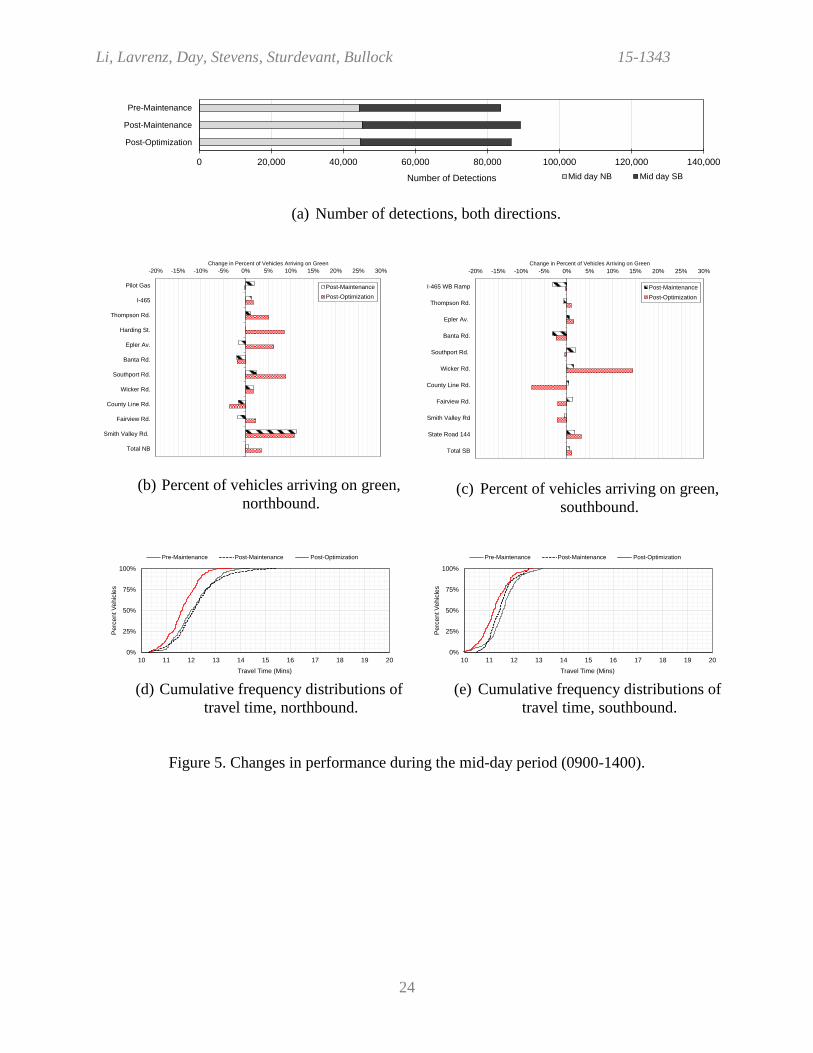
Mid-Day 20
The mid-day period experiences more modest gains in both POG (Figure 5b, Figure 5c) and 21
reduction in travel time (Figure 5d, Figure 5e). Overall, the corridor gains less than 1 percentage 22
point in both the northbound and southbound POG by maintenance alone. Optimization improves 23
the northbound POG by 3.5 points and the southbound by 1 point. Northbound arrivals see the 24
biggest gain at Smith Valley Road at 11 percentage points after maintenance, but a post-25
optimization increase of only 10 points, relative to the pre-maintenance period. This has been 26
offset by a slightly higher POG increase in the southbound approach at SR-144 during the same 27
period. The northbound travel time remains unchanged for the post-maintenance period, while 28
seeing a modest improvement of 0.3 minutes post-optimization. The southbound direction had 29
negligible improvements of 0.1 and 0.4 minutes at the median for post-maintenance and post-30
optimization periods, respectively. 31
Li, Lavrenz, Day, Stevens, Sturdevant, Bullock 15-1343
10
PM Peak 1
The PM peak period experiences the biggest increase in northbound POG again at Smith Valley 2
Road by 29 points post-maintenance and 28 points post-optimization, as seen in Figure 6b. Overall 3
however, these northbound gains are curbed by POG decreases at Fairview Road for post-4
maintenance, and I-465 and Epler Avenue for post-optimization. The overall northbound POG 5
increases by 1.8 and 3 percentage points, respectively, for post-maintenance and post-optimization. 6
In the southbound direction, the overall post-maintenance POG remains unchanged, while the 7
post-optimization results improve by an overall 3.4 percentage points, as shown in Figure 6c. 8
9
The travel time results during the PM peak period show that for the northbound direction, 10
maintenance improves travel time slightly more than optimization (Figure 6d). The median 11
northbound travel time post-maintenance is 0.7 minutes less than the baseline, while the post-12
optimization travel time is only 0.5 minutes less. This is due to the optimization heuristic favoring 13
the heavier southbound volumes (Figure 6a) and POG. However, as reflected in the southbound 14
travel time graph in Figure 6e, only marginal improvements of 0.4 minutes resulted from the 15
optimization, with negligible improvements by maintenance alone. For the slowest 20% of 16
travelers, both maintenance and optimization activities increased travel time in the southbound 17
direction compared to the baseline, signifying a reduction in arterial travel time reliability. 18
19
Statistical Significance of POG 20
A statistical test is conducted to determine whether the improvements in POG are significant for 21
post-maintenance and post-optimization from the pre-maintenance baseline for all time periods. A 22
one-sided significance test with consideration to the volume proportions of each scenario is 23
conducted with α = 0.05. For post-maintenance, nine, five, and eight approaches in the corridor 24
have significant improvements to the POG in the AM peak, mid-day, and PM peak, respectively 25
while three, seven, and twelve approaches have significant worsening of POG performance in the 26
AM peak, mid-day, and PM peak, respectively (Table 2a). For the post-optimization scenario, 27
twelve, ten, and eleven approaches improve in the AM peak, mid-day, and PM peak, respectively 28
while two, seven, and eight approaches worsen in the AM peak, mid-day, and PM peak, 29
respectively (Table 2b). The bulk of improvements from maintenance and optimization occur 30

Li, Lavrenz, Day, Stevens, Sturdevant, Bullock 15-1343
11
during the AM peak period, while there is more tradeoff between the northbound and southbound 1
approaches for the other two periods. 2
3
4
USER BENEFIT COST ESTIMATION 5
Signal timing maintenance and optimization almost invariably fall under the purview of some 6
public entity, whether it is the state DOT or a local municipal agency. Consequently, there are 7
significant benefits which can be calculated for the progression of vehicles through a corridor. The 8
most commonly considered of these benefits is the reduction in travel time for individual drivers. 9
This time savings can easily be monetized by determining a time value of money for passenger 10
cars and freight vehicles [15]. 11
12
Traditional user benefit calculations related to travel time savings have focused on the reduction 13
in average or median corridor travel time [16, 17]. However, there is increasing interest from 14
practitioners in also considering the impact of improvements in travel time reliability; that is, a 15
reduction in the variability of travel times around some central value. Prior study has shown that 16
consumers value improvements to travel time reliability at least as much, if not more so, than 17
actual reductions in travel time [18, 19, 20]. 18
19
In estimating user travel time benefits that result from the post-maintenance and post-optimization 20
scenarios, we incorporate both the monetary value of travel time savings and the value of 21
improvements in reliability, in a method known as the “mean-variance approach.” The mean-22
variance approach was utilized due to its explicit consideration of both measures of central 23
tendency and dispersion within the travel time distributions. While some measures (such as the 24
travel time/buffer/planning indices) describe travel time variability, they do not adequately convey 25
cases in which both travel time mean and variance are impacted. Similarly, mean-variance does 26
not provide the user with a direct comparison of travel time along the corridor relative to free flow 27
conditions. However, the principal interest in evaluating travel conditions in this study was relative 28
to the different maintenance scenarios, rather than against some baseline performance standard. 29
30

Li, Lavrenz, Day, Stevens, Sturdevant, Bullock 15-1343
12
The measure for travel time reliability is chosen to be the standard deviation of travel time through 1
the corridor, in line with this methodology [21, 22]. The travel time benefits for passenger and 2
commercial vehicles are computed as: 3
4
𝐵𝑒𝑛𝑒𝑓𝑖𝑡𝑖 = 𝑇𝑇𝑆𝑉𝑖 + 𝑇𝑇𝑅𝑉𝑖 (1) 5
Where 6
𝐵𝑒𝑛𝑒𝑓𝑖𝑡𝑖 = total travel time benefits for vehicle type i ($) 7
𝑇𝑇𝑆𝑉𝑖 = travel time savings value for vehicle type i ($) 8
𝑇𝑇𝑅𝑉𝑖 = travel time reliability value for vehicle type i ($) 9
And 10
𝑇𝑇𝑆𝑉𝑖 = ∆𝑇𝑇 ∗ 𝑉𝑜𝑙 ∗ 𝑃𝑖 ∗ 𝑂𝑐𝑐𝑖 ∗ 𝑇𝑇𝑉𝑖 ∗ 1 ℎ𝑟60 𝑚𝑖𝑛⁄ (2) 11
𝑇𝑇𝑅𝑉𝑖 = ∆𝑆𝐷 ∗ 𝑉𝑜𝑙 ∗ 𝑃𝑖 ∗ 𝑂𝑐𝑐𝑖 ∗ 𝑆𝐷𝑉𝑖 ∗ 1 ℎ𝑟60 𝑚𝑖𝑛⁄ (3) 12
Here, 13
∆𝑇𝑇 = The change in mean travel time along the corridor, as measured using crowd-14
sourced data (min) 15
∆𝑆𝐷 = The change in the standard deviation of travel time along the corridor (min) 16
𝑉𝑜𝑙 = The traffic volume through the corridor during the analysis period, measured using 17
count detectors on the intersection approaches (vehicles) 18
𝑃𝑖 = The percentage of the traffic stream that vehicle type i comprises 19
𝑂𝑐𝑐𝑖 = The average vehicle occupancy of vehicle type i (persons) 20
𝑇𝑇𝑉𝑖 = The time value of money for an individual in vehicle type i ($/person-hr) 21
𝑆𝐷𝑉𝑖 = The monetary value of a unit change in travel time standard deviation for an 22
individual in vehicle type i ($/person-hr) 23
24
In this analysis, two vehicle types are considered: passenger cars and commercial trucks. The value 25
of travel time, as well as the travel time savings estimation methodology are drawn from the latest 26
version of the Urban Mobility Report [23]. At present, the Urban Mobility Report does not provide 27
a direct way to monetize travel time reliability. However, a recent NCHRP report provides a ratio 28
of 1.3 for the value of a unit change in reliability to a unit change in actual travel time [24]. This 29
ratio is applied to the time value of money in the Urban Mobility Report to estimate the monetary 30

Li, Lavrenz, Day, Stevens, Sturdevant, Bullock 15-1343
13
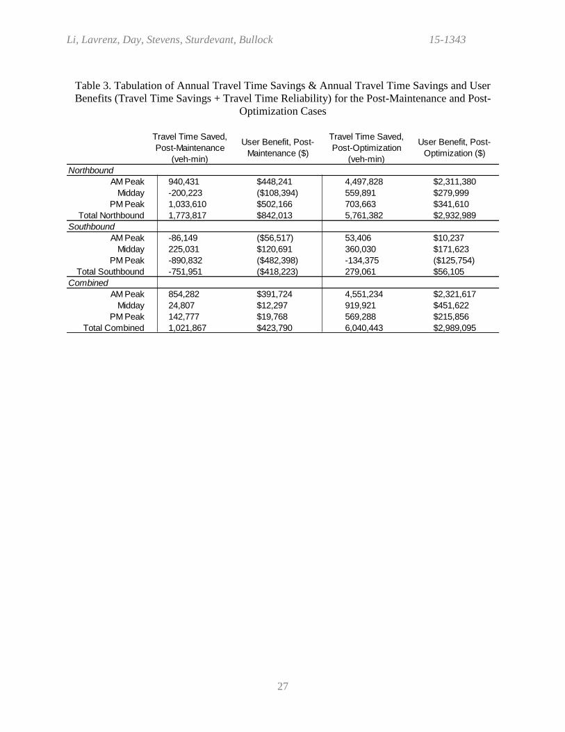
benefit of a change in travel time reliability. Table 3 provides a summary of the annual estimates 1
of travel time savings for weekday drivers, along with an estimation of the annual user travel time 2
benefits for the post-maintenance and post-optimization scenarios. Generally, it can be seen that 3
the largest user benefits accrue to northbound traffic during the morning period, with annual 4
benefits ranging from $448,241 to $2,311,380. 5
6
The impact of increased travel time and variability in certain periods for southbound traffic can 7
also be seen; traffic on the southbound lanes in the evening period saw increases in both average 8
travel times and travel time standard deviations, which is reflected in negative annual benefits (or 9
additional user costs) of $482,398 and $125,754 for post-maintenance and post-optimization, 10
respectively. Overall, however, the benefits of signal maintenance and optimization has a net 11
positive effect, with combined annual benefits for both directions totaling $423,473 for post-12
maintenance, and $2,989,095 for post-optimization. 13
14
Figure 7 provides a further breakdown of the user benefits attributable to changes in travel time 15
and travel time reliability. Here, the column charts show the same “total benefit” values for each 16
time period and direction as presented in Table 3. Additionally, the separate “time savings 17
benefit” and “reliability” benefit are displayed for each case. In Figure 7b for example, it is 18
evident that a majority of user benefits in the corridor were accrued for the northbound direction 19
during the AM period of the post-optimization scenario. Roughly 60% of this benefit was from 20
travel time savings, while the remainder was due to significant increases in travel time reliability 21
(that is, a decrease in standard deviation). 22
23
It can also be seen that for a number of other cases, such as the mid-day period of the post-24
optimization scenario (Figure 7d), travel time reliability comprised a substantial amount of the 25
total user benefit, relative to travel time savings. In several instances, such the southbound lanes 26
during the PM peak period of the post-optimization scenario (Figure 7f), a worsening of travel 27
time reliability actually changed the net user benefit to a negative value, relative to the benefits 28
that resulted only from reductions in travel time. 29
30
Li, Lavrenz, Day, Stevens, Sturdevant, Bullock 15-1343
14
It can be seen that for the post-maintenance scenario in Figure 7a, the effect of increased reliability 1
for the northbound lanes is modest relative to reductions in average travel time. Conversely, while 2
the southbound lanes see only a slight increase in average travel time, there is a larger increase in 3
travel time variance (standard deviation), with this measure capturing most of the negative benefits 4
as shown in Table 3. For the post-optimization scenario in Figure 7b, it can be seen that the impact 5
of increased travel time reliability for the northbound lanes has nearly the same benefit as the 6
actual travel time savings; for the combined benefits of both directions, increased travel time 7
reliability still carries substantial value to the end user. 8
9
CONCLUSIONS 10
Percentage of vehicles arriving on green and vehicle travel times for a section of SR-37 south of 11
Indianapolis were evaluated for three separate scenarios in 2013. The pre-maintenance baseline 12
data assessed the corridor without changes to signal timing. After the time-of-day plans were 13
aligned and controller clocks were synchronized, the post-maintenance median travel times saw 14
modest reductions in the northbound direction by 0.9 minutes in the AM peak period. The 15
progression-optimized offsets provided the greatest reductions in travel time, with a median of 2 16
minutes for the northbound AM peak over the pre-maintenance scenario. The improvements to 17
percent of green arrivals were also found to be statistically significant for that period. The PM peak 18
saw a more modest improvement of 0.7 minutes in the northbound direction after optimization. 19
However, both after-scenarios resulted in less reliable travel times for the heavy southbound PM 20
peak flows, especially for the slowest 20% of travelers. There were more tradeoffs in arrivals on 21
green between northbound and southbound approaches throughout the corridor in the PM peak as 22
a result of maintenance and optimization. 23
24
Using the mean-variance user benefit calculation method, which accounted for both median travel 25
time and travel time reliability, the user benefit accrued for maintenance-only tasks was $423,473 26
for all weekdays in one year. Benefits as a result of optimization activities were substantially 27
higher, totaling $2,989,095 for all weekdays in one year. This study has shown that a non-trivial 28
amount of user benefit can be derived simply by performing time-of-day and clock maintenance 29
tasks; additional positive impact can be demonstrated in future research through measures such as 30

Li, Lavrenz, Day, Stevens, Sturdevant, Bullock 15-1343
15
fuel savings and emissions reductions associated with this maintenance. These maintenance 1
activities are also crucial for accurately performing optimization tasks that do not involve new 2
equipment or infrastructure investments. Moreover, progression optimization may come with 3
additional agency time and resource costs which may not be practical at all locations. Future 4
research may leverage methods similar to the mean-variance approach to monetize the value of 5
these maintenance and optimization activities. This valuation, based on objective measures of 6
travel time and travel time reliability improvements, will serve as a strongly defensible metric for 7
continuing the development of integrated signal optimization tasks based on high-resolution 8
controller and crowd-sourced probe vehicle data. 9
10
ACKNOWLEDGEMENT 11
The data source used for this paper was provided by INRIX. This work was supported in part by 12
the Joint Transportation Research Program and Pooled Fund Study (TPF-5(258)) led by the 13
Indiana Department of Transportation (INDOT) and supported by the state transportation agencies 14
of California, Georgia, Kansas, Minnesota, Mississippi, New Hampshire, Pennsylvania, Texas, 15
Utah, and Wisconsin, the Federal Highway Administration Arterial Management Program, and the 16
Chicago Department of Transportation. The contents of this paper reflect the views of the authors, 17
who are responsible for the facts and the accuracy of the data presented herein, and do not 18
necessarily reflect the official views or policies of the sponsoring organizations. These contents do 19
not constitute a standard, specification, or regulation. 20

Li, Lavrenz, Day, Stevens, Sturdevant, Bullock 15-1343
16
REFERENCES
1. 1. Dowling, R.G., W.K. Cheng. “Evaluation of Speed Measurement and Prediction
Techniques for Signalized Arterials.” Transportation Research Record, n. 1564, pp. 20-29,
1996.
2. Wasson, Jayson S. J.R. Sturdevant, D.M. Bullock. “Real-time Travel Time Estimates Using
Media Access Control Address Matching.” ITE Journal, v. 78, n. 6, pp. 20-23, June 2008.
3. Liu, H.X., W. Ma. “A virtual vehicle probe model for time-dependent travel time estimation
on signalized arterials.” Transportation Research Part C: Emerging Technologies, v. 17, n. 1,
pp. 11-26, 2009.
4. Day, C.M., R. Haseman, H. Premachandra, T.M. Brennan, J.S. Wasson, J. R. Sturdevant, and
D.M. Bullock. “Evaluation of Arterial Signal Coordination: Methodologies for Visualizing
High-Resolution Event Data and Measuring Travel Time.” Transportation Research Record
No. 2192, pp. 37-49, 2010.
5. Day, C. M., D. M. Bullock, H. Li, S. M. Remias, A. M. Hainen, R. S. Freije, A. L. Stevens, J.
R. Sturdevant, and T. M. Brennan. “Performance Measures for Traffic Signal Systems: An
Outcome-Oriented Approach.” Purdue University, West Lafayette, Indiana, 2014. doi:
10.5703/1288284315333.
6. Wu, X., D. M. Levinson, H. X. Liu. “Perception of Waiting Time at Signalized
Intersections.” Transportation Research Record, n. 2135, pp. 52-59, 2009.
7. Wang, Y. et al. “Which phone will you get next: observing trends and predicting the choice.”
IEEE/IFIP Network Operations and Management Symposium (NOMS), pp. 7, 2014
8. Day, C.M., T.M. Brennan, A.M. Hainen, S.M. Remias, H. Premachandra, J.R. Sturdevant, G.
Richards, J.S. Wasson, and D.M. Bullock. “Reliability, Flexibility, and Environmental
Impact of Alternative Objective Functions for Arterial Offset Optimization.” Transportation
Research Record No. 2259, pp. 8-22, 2011.
9. Chen, W., L. Henley, J. Price. “Assessment of Traffic Signal Maintenance and Operations
Needs at Virginia Department of Transportation.” Transportation Research Record, n. 2128,
pp. 11-19, 2009.
10. Kergaye, C., A. Stevanoic, P. T. Martin. “Comparison of Before–After Versus Off–On
Adaptive Traffic Control Evaluations.” Transportation Research Record, n. 2128, pp. 192-
201, 2009.
11. Day, C.M. and D.M. Bullock. “Computational Efficiency of Alternative Algorithms for
Arterial Offset Optimization.” Transportation Research Record No. 2259, pp. 37-47, 2011.
12. Remias, S. M. et al. “Performance Characterization of Arterial Traffic Flow with Probe
Vehicle Data.” Transportation Research Record, n. 2380, pp. 10-21, 2013.
13. Kell, J. H., I. J. Fullerton, and M. K. Mills. Traffic Detector Handbook, 2d ed. Report
FHWA-IP-90-002. FHWA, U.S. Department of Transportation, July 1990.
14. Traffic Signal Timing Manual. Publication No. FHWA-HOP-08-024, Section 6.6, 2008.
15. K. Sinha and S. Labi, Transportation Decision Making: Principles of Project Evaluation and
Programming, Hoboken, New Jersey: John Wiley & Sons, Inc., 2007.
16. Kittleson & Associates, Inc., "SHRP 2 Project L17 Guidebook: Placing a Value on Travel-
Time Reliability," Transportation Research Board of the National Academies, Washington,
DC, 2013.
17. Litman, T. ""Travel Time", Transportation Cost and Benefit Analysis." 2009. [Online].
Available: http://www.vtpi.org/tca/tca0502.pdf.

Li, Lavrenz, Day, Stevens, Sturdevant, Bullock 15-1343
17
18. Noland, R., K. Small. "Travel-time Uncertainty, Departure Time Choice, and the Cost of
Morning Commutes." Transportation Research Record, v. 1493, pp. 150-158, 1995.
19. De Jong, G., S. Bakker, M. Pieters and P. Wortelboer-van Donselaar. "New Values of Time
and Reliability in Freight Transport in the Netherlands." AVV Transport Research Centre,
Dutch Ministry of Transport, Public Works and Water Management, Rotterdam, 2004.
20. Fosgerau, M., K. Hjorth, C. Brems and D. Fukuda, "Travel Time Variability - Definition and
Valuation." Danish Department of Transport, Copenhagen, 2008.
21. Jackson, W. and J. Jucker, "An Empirical Study of Travel Time Variability and Travel
Choice behavior." Transportation Science, v. 16, pp. 460-475, 1982.
22. Cambridge Systematics, ICF International, "Value of Travel Time Reliability: Synthesis
Report & Workshop Working Paper." SHRP 2 Workshop on the Value of Travel Time
Reliability, Washington, DC, 2012.
23. Schrank, D., B. Eisele and T. Lomax, "The Urban Mobility Report." Texas A&M
Transportation Institute, 2012.
24. Small, K., R. Noland, X. Chiu and D. Lewis, "NCHRP Report 431 - Valuation of Travel
Time Savings and Predictability in Congested Conditions for Highway User-Cost
Estimation." Transportation Research Board of the National Academies, Washington, DC,
1999.

Li, Lavrenz, Day, Stevens, Sturdevant, Bullock 15-1343
18
FIGURES AND TABLES
Figures
Figure 1. Map overview. ............................................................................................................... 19
Figure 2. Time-of-day plan compatibility assessment of intersections, shaded by cycle length. 21
Figure 3. Web-based application to optimize signal offsets for progression. ............................... 22
Figure 4. Changes in performance during the AM peak period (0600-0900). ............................. 23
Figure 5. Changes in performance during the mid-day period (0900-1400). ............................... 24
Figure 6. Changes in performance during the PM peak period (1400-1900). .............................. 25
Figure 7. Comparison of annual travel time savings benefits, travel time reliability benefits, and
total benefits. .......................................................................................................................... 28
Tables
Table 1. Detection and phasing inventory of study corridor. ....................................................... 20
Table 2. Statistical significance (α = 0.05) of changes in POG. ................................................... 26
Table 3. Tabulation of Annual Travel Time Savings & Annual Travel Time Savings and User
Benefits (Travel Time Savings + Travel Time Reliability) for the Post-Maintenance and
Post-Optimization Cases ........................................................................................................ 27

Li, Lavrenz, Day, Stevens, Sturdevant, Bullock 15-1343
19
(a) Corridor location within Indiana.
(c) Southern portion of corridor
(b) Northern portion of corridor.
Figure 1. Map overview.
Corridor Location
12. State Road 144
11. Smith Valley Rd.
10. Fairview Rd.
9. County Line Rd.
8. Wicker Rd.
7. Southport Rd.
6. Banta Rd.
5. Epler Av.
5540 ft
2660 ft
5840 ft
2900 ft
5490 ft
5660 ft
16500 ft
4. Harding St.
3. Thompson Rd.
2. I-465 Ramps
2470 ft to Epler Av.
1. Pilot Gas
860 ft
950 ft
640 ft

Li, Lavrenz, Day, Stevens, Sturdevant, Bullock 15-1343
20
Table 1. Detection and phasing inventory of study corridor.
* Two intersections using a single controller.
Intersection Identification No. Channels Phase Channels Phase
1. Pilot Gas 4493 5, 6, 9 2 -- --
37, 38 Overlap B 41, 42, 45 Overlap F
1, 2, 5, 6 Overlap G 21, 22 Overlap A
3. Thompson Rd. 2028 5, 6, 9, 10 2 22, 25, 26 6
4. Harding St. 2153 2, 5, 6 2 -- --
5. Epler Av. 2138 5, 6, 9 2 14, 17, 18 6
6. Banta Rd. 4414 17, 18 6 19, 20 2
7. Southport Rd. 4437 2 6 13 2
8. Wicker Rd. 4443 2, 4 2 8, 10 6
9. County Line Rd. 4431 9 6 13 2
10. Fairview Rd. 4413 10, 11 6 5, 16 2
11. Smith Valley Rd. 4469 6 6 2 2
12. State Road 144 4458 -- -- 13, 14 2
Northbound Southbound
2. I-465* 2077

Li, Lavrenz, Day, Stevens, Sturdevant, Bullock 15-1343
21
(a) Before alignment.
(b) After alignment.
Figure 2. Time-of-day plan compatibility assessment of intersections, shaded by cycle length.
0 3 6 9 12 15 18 21
Time of Day
State Road 144
Smith Valley Rd.
Fairview Rd.
County Line Rd.
Wicker Rd.
Southport Rd.
Banta Rd.
Epler Av.
Harding St.
Thompson Rd.
I-465
Pilot Gas
State Road 144
Smith Valley Rd.
Fairview Rd.
County Line Rd.
Wicker Rd.
Southport Rd.
Banta Rd.
Epler Av.
Harding St.
Thompson Rd.
I-465
Pilot Gas
FREE 120 Seconds 80 Seconds 40 Seconds
AM peak Mid-day PM peak

Li, Lavrenz, Day, Stevens, Sturdevant, Bullock 15-1343
22
Figure 3. Web-based application to optimize signal offsets for progression.
i
ii iii

Li, Lavrenz, Day, Stevens, Sturdevant, Bullock 15-1343
23
(a) Number of detections, both directions.
(b) Percent of vehicles arriving on green,
northbound.
(c) Percent of vehicles arriving on green,
southbound.
(d) Cumulative frequency distributions of
travel time, northbound.
(e) Cumulative frequency distributions of
travel time, southbound.
Figure 4. Changes in performance during the AM peak period (0600-0900).
0 20,000 40,000 60,000 80,000 100,000 120,000 140,000
Post-Optimization
Post-Maintenance
Pre-Maintenance
Number of Detections AM NB AM SB
-20% -15% -10% -5% 0% 5% 10% 15% 20% 25% 30%
Pilot Gas
I-465
Thompson Rd.
Harding St.
Epler Av.
Banta Rd.
Southport Rd.
Wicker Rd.
County Line Rd.
Fairview Rd.
Smith Valley Rd.
Total NB
Change in Percent of Vehicles Arriving on Green
Post-Maintenance
Post-Optimization
-20% -15% -10% -5% 0% 5% 10% 15% 20% 25% 30%
I-465 WB Ramp
Thompson Rd.
Epler Av.
Banta Rd.
Southport Rd.
Wicker Rd.
County Line Rd.
Fairview Rd.
Smith Valley Rd
State Road 144
Total SB
Change in Percent of Vehicles Arriving on Green
Post-Maintenance
Post-Optimization
0%
25%
50%
75%
100%
10 11 12 13 14 15 16 17 18 19 20
Pe
rce
nt V
eh
icle
s
Travel Time (Mins)
Pre-Maintenance Post-Maintenance Post-Optimization
0%
25%
50%
75%
100%
10 11 12 13 14 15 16 17 18 19 20
Pe
rce
nt V
eh
icle
s
Travel Time (Mins)
Pre-Maintenance Post-Maintenance Post-Optimization
Li, Lavrenz, Day, Stevens, Sturdevant, Bullock 15-1343
24
(a) Number of detections, both directions.
(b) Percent of vehicles arriving on green,
northbound.
(c) Percent of vehicles arriving on green,
southbound.
(d) Cumulative frequency distributions of
travel time, northbound.
(e) Cumulative frequency distributions of
travel time, southbound.
Figure 5. Changes in performance during the mid-day period (0900-1400).
0 20,000 40,000 60,000 80,000 100,000 120,000 140,000
Post-Optimization
Post-Maintenance
Pre-Maintenance
Number of Detections Mid day NB Mid day SB
-20% -15% -10% -5% 0% 5% 10% 15% 20% 25% 30%
Pilot Gas
I-465
Thompson Rd.
Harding St.
Epler Av.
Banta Rd.
Southport Rd.
Wicker Rd.
County Line Rd.
Fairview Rd.
Smith Valley Rd.
Total NB
Change in Percent of Vehicles Arriving on Green
Post-Maintenance
Post-Optimization
-20% -15% -10% -5% 0% 5% 10% 15% 20% 25% 30%
I-465 WB Ramp
Thompson Rd.
Epler Av.
Banta Rd.
Southport Rd.
Wicker Rd.
County Line Rd.
Fairview Rd.
Smith Valley Rd
State Road 144
Total SB
Change in Percent of Vehicles Arriving on Green
Post-Maintenance
Post-Optimization
0%
25%
50%
75%
100%
10 11 12 13 14 15 16 17 18 19 20
Pe
rcen
t V
eh
icle
s
Travel Time (Mins)
Pre-Maintenance Post-Maintenance Post-Optimization
0%
25%
50%
75%
100%
10 11 12 13 14 15 16 17 18 19 20
Pe
rcen
t V
eh
icle
s
Travel Time (Mins)
Pre-Maintenance Post-Maintenance Post-Optimization

Li, Lavrenz, Day, Stevens, Sturdevant, Bullock 15-1343
25
(a) Number of detections, both directions.
(b) Percent of vehicles arriving on green,
northbound.
(c) Percent of vehicles arriving on green,
southbound.
(d) Cumulative frequency distributions of
travel time, northbound.
(e) Cumulative frequency distributions of
travel time, southbound.
Figure 6. Changes in performance during the PM peak period (1400-1900).
0 20,000 40,000 60,000 80,000 100,000 120,000 140,000
Post-Optimization
Post-Maintenance
Pre-Maintenance
Number of Detections PM NB PM SB
-20% -15% -10% -5% 0% 5% 10% 15% 20% 25% 30%
Pilot Gas
I-465
Thompson Rd.
Harding St.
Epler Av.
Banta Rd.
Southport Rd.
Wicker Rd.
County Line Rd.
Fairview Rd.
Smith Valley Rd.
Total NB
Change in Percent of Vehicles Arriving on Green
Post-Maintenance
Post-Optimization
-20% -15% -10% -5% 0% 5% 10% 15% 20% 25% 30%
I-465 WB Ramp
Thompson Rd.
Epler Av.
Banta Rd.
Southport Rd.
Wicker Rd.
County Line Rd.
Fairview Rd.
Smith Valley Rd
State Road 144
Total SB
Change in Percent of Vehicles Arriving on Green
Post-Maintenance
Post-Optimization
0%
25%
50%
75%
100%
10 11 12 13 14 15 16 17 18 19 20
Pe
rcen
t V
eh
icle
s
Travel Time (Mins)
Pre-Maintenance Post-Maintenance Post-Optimization
0%
25%
50%
75%
100%
10 11 12 13 14 15 16 17 18 19 20
Pe
rcen
t V
eh
icle
s
Travel Time (Mins)
Pre-Maintenance Post-Maintenance Post-Optimization

Li, Lavrenz, Day, Stevens, Sturdevant, Bullock 15-1343
26
Table 2. Statistical significance (α = 0.05) of changes in POG.
(a) Post-maintenance from pre-maintenance.
(b) Post-optimization from pre-maintenance.
Z-Score P-Value Improved? Worsened? Z-Score P-Value Improved? Worsened? Z-Score P-Value Improved? Worsened?
Pilot Gas (NB) -1.65412 0.049 No Yes 1.54262 0.061 No No 2.15865 0.015 Yes No
I-465 WB Ramp (NB) -0.24683 0.403 No No -3.55828 0.000 No Yes -10.85279 0.000 No Yes
I-465 WB Ramp (SB) 0.20718 0.418 No No -2.13899 0.016 No Yes -0.16526 0.434 No No
I-465 EB Ramp (NB) 2.95039 0.002 Yes No 1.15711 0.124 No No -0.22255 0.412 No No
I-465 EB Ramp (SB) -0.27907 0.390 No No -1.90701 0.028 No Yes -9.10254 0.000 No Yes
Thompson Rd. (NB) 2.86528 0.002 Yes No 1.23387 0.109 No No 2.69044 0.004 Yes No
Thompson Rd. (SB) 2.74163 0.003 Yes No -0.61635 0.269 No No -1.66760 0.048 No Yes
Harding St. (NB) -1.69198 0.045 No Yes -0.12112 0.452 No No 3.68708 0.000 Yes No
Epler Av. (NB) 1.08720 0.138 No No -1.63804 0.051 No No -2.29138 0.011 No Yes
Epler Av. (SB) 0.24312 0.404 No No 0.61853 0.268 No No -8.09132 0.000 No Yes
Banta Rd. (NB) -0.78828 0.215 No No -3.18132 0.001 No Yes 8.45821 0.000 Yes No
Banta Rd. (SB) 0.43493 0.332 No No -5.54012 0.000 No Yes 5.11448 0.000 Yes No
Southport Rd. (NB) 1.49615 0.067 No No 1.96719 0.025 Yes No 2.55545 0.005 Yes No
Southport Rd. (SB) -0.07790 0.469 No No 1.52909 0.063 No No -3.10472 0.001 No Yes
Wicker Rd. (NB) 6.26022 0.000 Yes No 2.28692 0.011 Yes No -3.03842 0.001 No Yes
Wicker Rd. (SB) 0.03396 0.486 No No 1.50479 0.066 No No -4.16198 0.000 No Yes
County Line Rd. (NB) 6.07302 0.000 Yes No -2.09974 0.018 No Yes -1.13141 0.129 No No
County Line Rd. (SB) -0.25856 0.398 No No 0.75509 0.225 No No -2.05252 0.020 No Yes
Fairview Rd. (NB) -4.91025 0.000 No Yes -2.24999 0.012 No Yes -8.98787 0.000 No Yes
Fairview Rd. (SB) 7.37278 0.000 Yes No 2.00471 0.022 Yes No -1.73244 0.042 No Yes
Smith Valley Rd. (NB) 13.90282 0.000 Yes No 9.86392 0.000 Yes No 24.47125 0.000 Yes No
Smith Valley Rd. (SB) 1.82962 0.034 Yes No -0.42191 0.337 No No 3.92685 0.000 Yes No
SR 144 (SB) 4.86363 0.000 Yes No 1.71142 0.044 Yes No -1.80289 0.036 No Yes
PM Peak (1400 - 1900)AM Peak (0600 - 0900) Mid-Day (0900 - 1400)
Approach
Z-Score P-Value Improved? Worsened? Z-Score P-Value Improved? Worsened? Z-Score P-Value Improved? Worsened?
Pilot Gas (NB) -0.62239 0.267 No No -0.17544 0.430 No No -0.22878 0.410 No No
I-465 WB Ramp (NB) 0.31330 0.377 No No -3.15039 0.001 No Yes -6.59831 0.000 No Yes
I-465 WB Ramp (SB) 1.00956 0.156 No No -0.21023 0.417 No No 1.64209 0.050 No No
I-465 EB Ramp (NB) 2.30414 0.011 Yes No 1.51906 0.064 No No -6.84866 0.000 No Yes
I-465 EB Ramp (SB) 0.45019 0.326 No No -2.04737 0.020 No Yes -3.87003 0.000 No Yes
Thompson Rd. (NB) 6.69938 0.000 Yes No 5.54876 0.000 Yes No 2.59677 0.005 Yes No
Thompson Rd. (SB) 0.90688 0.182 No No 0.89955 0.184 No No 8.37191 0.000 Yes No
Harding St. (NB) 2.69696 0.003 Yes No 10.44737 0.000 Yes No 5.09669 0.000 Yes No
Epler Av. (NB) 1.02586 0.152 No No 6.95326 0.000 Yes No -14.00992 0.000 No Yes
Epler Av. (SB) -4.48713 0.000 No Yes 1.65417 0.049 Yes No -3.60227 0.000 No Yes
Banta Rd. (NB) -0.75053 0.226 No No -3.04939 0.001 No Yes 10.03601 0.000 Yes No
Banta Rd. (SB) -1.63626 0.051 No No -4.14688 0.000 No Yes 11.02179 0.000 Yes No
Southport Rd. (NB) 3.91313 0.000 Yes No 7.12701 0.000 Yes No -3.21919 0.001 No Yes
Southport Rd. (SB) 8.35780 0.000 Yes No -0.33049 0.371 No No -0.72221 0.235 No No
Wicker Rd. (NB) 7.62963 0.000 Yes No 2.32694 0.010 Yes No -0.16323 0.435 No No
Wicker Rd. (SB) 11.78819 0.000 Yes No 16.27737 0.000 Yes No 2.80638 0.003 Yes No
County Line Rd. (NB) 7.68108 0.000 Yes No -4.28901 0.000 No Yes -4.46305 0.000 No Yes
County Line Rd. (SB) -12.24148 0.000 No Yes -9.97269 0.000 No Yes 4.93974 0.000 Yes No
Fairview Rd. (NB) 0.94372 0.173 No No 2.81420 0.002 Yes No 22.99020 0.000 Yes No
Fairview Rd. (SB) 8.37791 0.000 Yes No -2.65259 0.004 No Yes -2.66271 0.004 No Yes
Smith Valley Rd. (NB) 15.59135 0.000 Yes No 9.35042 0.000 Yes No 23.85304 0.000 Yes No
Smith Valley Rd. (SB) 4.14156 0.000 Yes No -1.44246 0.075 No No 2.56236 0.005 Yes No
SR 144 (SB) 8.77263 0.000 Yes No 3.13884 0.001 Yes No 16.16597 0.000 Yes No
PM Peak (1400 - 1900)Mid-Day (0900 - 1400)AM Peak (0600 - 0900)
Approach
Li, Lavrenz, Day, Stevens, Sturdevant, Bullock 15-1343
27
Table 3. Tabulation of Annual Travel Time Savings & Annual Travel Time Savings and User
Benefits (Travel Time Savings + Travel Time Reliability) for the Post-Maintenance and Post-
Optimization Cases
Travel Time Saved,
Post-Maintenance
(veh-min)
User Benefit, Post-
Maintenance ($)
Travel Time Saved,
Post-Optimization
(veh-min)
User Benefit, Post-
Optimization ($)
Northbound
AM Peak 940,431 $448,241 4,497,828 $2,311,380
Midday -200,223 ($108,394) 559,891 $279,999
PM Peak 1,033,610 $502,166 703,663 $341,610
Total Northbound 1,773,817 $842,013 5,761,382 $2,932,989
Southbound
AM Peak -86,149 ($56,517) 53,406 $10,237
Midday 225,031 $120,691 360,030 $171,623
PM Peak -890,832 ($482,398) -134,375 ($125,754)
Total Southbound -751,951 ($418,223) 279,061 $56,105
Combined
AM Peak 854,282 $391,724 4,551,234 $2,321,617
Midday 24,807 $12,297 919,921 $451,622
PM Peak 142,777 $19,768 569,288 $215,856
Total Combined 1,021,867 $423,790 6,040,443 $2,989,095

Li, Lavrenz, Day, Stevens, Sturdevant, Bullock 15-1343
28
(a) Post-maintenance, AM peak.
(b) Post-optimization, AM peak.
(c) Post-maintenance, mid-day.
(d) Post-optimization, mid-day.
(e) Post-maintenance, PM peak.
(f) Post-optimization, PM peak.
Figure 7. Comparison of annual travel time savings benefits, travel time reliability benefits, and
total benefits.
-$500,000
$0
$500,000
$1,000,000
$1,500,000
$2,000,000
$2,500,000
Northbound Southbound Combined-$500,000
$0
$500,000
$1,000,000
$1,500,000
$2,000,000
$2,500,000
Northbound Southbound Combined
-$500,000
$0
$500,000
$1,000,000
$1,500,000
$2,000,000
$2,500,000
Northbound Southbound Combined
Time Savings Benefit
Reliability Benefit
Total Benefit
-$500,000
$0
$500,000
$1,000,000
$1,500,000
$2,000,000
$2,500,000
Northbound Southbound Combined
-$500,000
$0
$500,000
$1,000,000
$1,500,000
$2,000,000
$2,500,000
Northbound Southbound Combined-$500,000
$0
$500,000
$1,000,000
$1,500,000
$2,000,000
$2,500,000
Northbound Southbound Combined