1

Quantification of additive manufacturing induced variations in

the global and local performance characteristics of a complex

multi-stage control valve trim

Dharminder Singha*, Matthew Charltonb, Taimoor Asimc, Rakesh Mishraa, Andrew Townsenda, Liam Blunta

aSchool of Computing & Engineering, University of Huddersfield, Queensgate, Huddersfield HD1 3DH, United

Kingdom

bPreviously Manager of Product Development, Trillium Flow Technologies, Britannia House, Huddersfield

Road, Elland HX5 9JR, United Kingdom

cSchool of Engineering, Robert Gordon University, Garthdee Road, Aberdeen AB10 7GJ, United Kingdom

Abstract

Control valves that are used in severe service applications have trim cages that are

geometrically quite complex. Most of these trims are manufactured using traditional

manufacturing methods which are expensive and time-consuming. In order to reduce

manufacturing costs and shorten the product development cycles, Additive Manufacturing

(AM) methods have been gaining popularity over the traditional manufacturing methods.

Selective Laser Melting (SLM) is one of the most popular AM techniques. In this paper, the

effect of the conventional Electron Discharge Machining (EDM) method and the SLM

method on the performance characteristics of a complex multi-stage disc stack trim is

investigated. Experimental tests conducted on the SLM trim showed that the flow capacity

reduced in comparison to the EDM manufactured trim. Surface profile measurements

indicated that the surface roughness of the SLM trim was significantly higher than the EDM

trim. In order to evaluate the effect of surface roughness on performance in detail, well

validated numerical simulations were conducted to compare the local performance of the

valve trims manufactured by the two methods. The simulation results showed that the wall

shear stress increases by 1.9 times on the trim manufactured by the SLM method due to the

increased roughness.

Keywords: Additive manufacturing; Selective laser melting; Control valves; Surface

roughness; Computation Fluid Dynamics (CFD); Flow capacity

1. Introduction

Control valves are one of the most critical and complex components of process control

systems. They are designed to control process parameters such as flow rate, pressure,

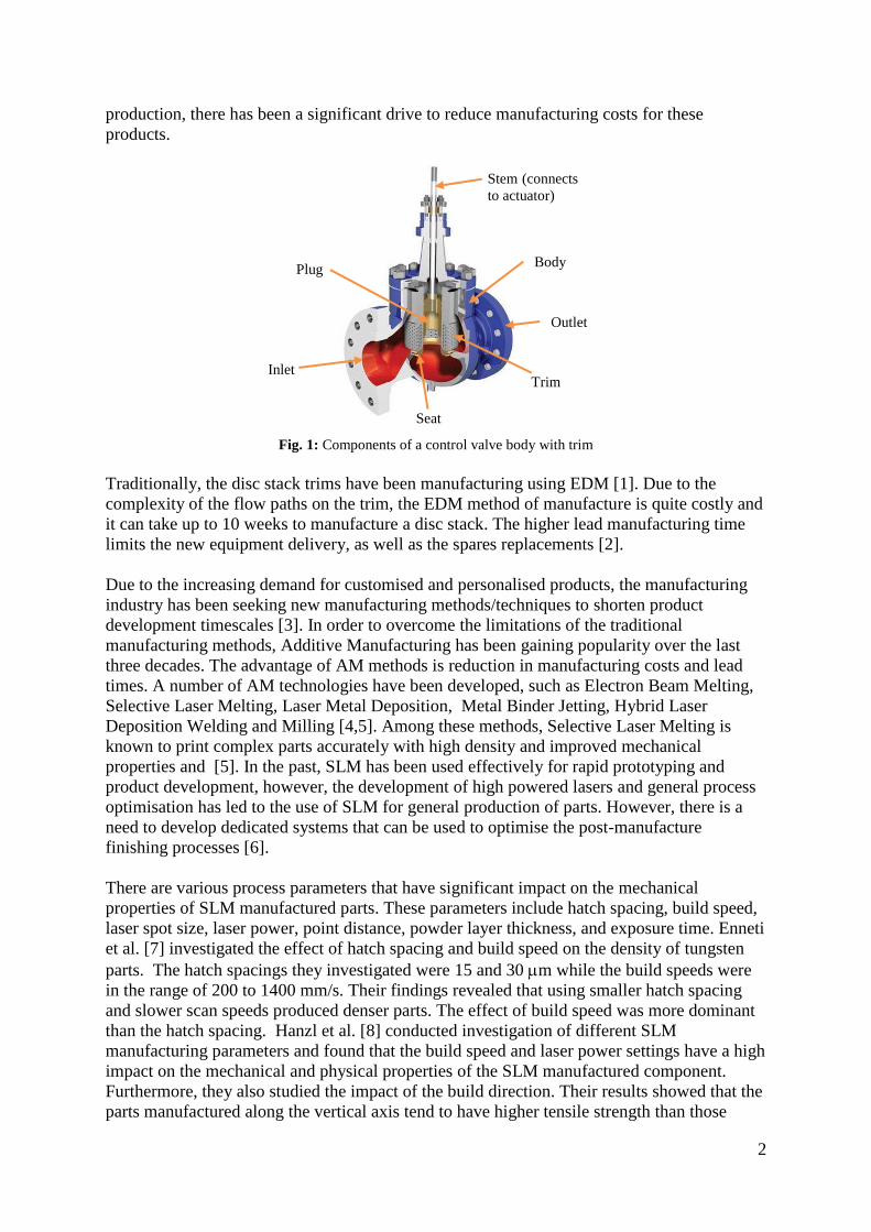
temperature, etc. The components of a control valve are shown in Fig. 1. Flow control is

achieved by varying the flow area by controlling the position of a plug against a seat inside a

cage/stack. The cage is composed of a number of discs stacked together that incorporate

provisions for complex fluid flow paths on their surface. This is achieved by incorporating

well designed obstructions in the flow paths to induce a controlled amount of energy loss.

The discs are designed to provide pressure drop in a number of stages, where the flow area is

expanded after the pressure drop at each stage and effectively reducing the fluid velocity

across the surface of the disc in order to prevent problems like noise, cavitation and erosion.

There have been significant developments in the design of severe service control valves over

the past two decades from their initial concept designs. As the number of services that require

these type of control valves continues to increase and due to the associated costs of

2

production, there has been a significant drive to reduce manufacturing costs for these

products.

Fig. 1: Components of a control valve body with trim

Traditionally, the disc stack trims have been manufacturing using EDM [1]. Due to the

complexity of the flow paths on the trim, the EDM method of manufacture is quite costly and

it can take up to 10 weeks to manufacture a disc stack. The higher lead manufacturing time

limits the new equipment delivery, as well as the spares replacements [2].

Due to the increasing demand for customised and personalised products, the manufacturing

industry has been seeking new manufacturing methods/techniques to shorten product

development timescales [3]. In order to overcome the limitations of the traditional

manufacturing methods, Additive Manufacturing has been gaining popularity over the last

three decades. The advantage of AM methods is reduction in manufacturing costs and lead

times. A number of AM technologies have been developed, such as Electron Beam Melting,

Selective Laser Melting, Laser Metal Deposition, Metal Binder Jetting, Hybrid Laser

Deposition Welding and Milling [4,5]. Among these methods, Selective Laser Melting is

known to print complex parts accurately with high density and improved mechanical

properties and [5]. In the past, SLM has been used effectively for rapid prototyping and

product development, however, the development of high powered lasers and general process

optimisation has led to the use of SLM for general production of parts. However, there is a

need to develop dedicated systems that can be used to optimise the post-manufacture

finishing processes [6].

There are various process parameters that have significant impact on the mechanical

properties of SLM manufactured parts. These parameters include hatch spacing, build speed,

laser spot size, laser power, point distance, powder layer thickness, and exposure time. Enneti

et al. [7] investigated the effect of hatch spacing and build speed on the density of tungsten

parts. The hatch spacings they investigated were 15 and 30 m while the build speeds were

in the range of 200 to 1400 mm/s. Their findings revealed that using smaller hatch spacing

and slower scan speeds produced denser parts. The effect of build speed was more dominant

than the hatch spacing. Hanzl et al. [8] conducted investigation of different SLM

manufacturing parameters and found that the build speed and laser power settings have a high

impact on the mechanical and physical properties of the SLM manufactured component.

Furthermore, they also studied the impact of the build direction. Their results showed that the

parts manufactured along the vertical axis tend to have higher tensile strength than those

Inlet

Outlet

Trim

Plug

Stem (connects

to actuator)

Body

Seat

3

manufactured along the horizontal axis. Building at an angle of less than 45° caused

delamination of the layers and deteriorated the components’ mechanical properties.

Osakada and Shiomi [9] investigated the deformation of SLM manufactured parts caused by

thermal distortion using Finite Element Analysis. Their findings show that there is an

increase in the degree of thermal distortion of a single layer with increase in the length of

scanning track and thus, there is an increase in the maximum tensile stress. They suggested

that during the formation of a large layer on the powder bed, the forming area should be

divided into a number of small segments. Rapid heating and cooling of the part induces

residual stresses within the part. Osakada and Shiomi [9] discovered that residual tensile

stresses have a large effect on the deformities produced on the manufactured part. They also

found large residual tensile stresses are present in the top layers of the model which decrease

rapidly as the distance from the model’s top surface increases. Based on these findings, the

authors suggested that re-scanning during each layer formation can reduce the residual

stresses. This provides more optimised control over the applied heat on the component, thus

the manufacturing speed reduces and rapid heating is prevented. Build speed is, therefore, a

very important parameter that needs to be considered, especially when manufacturing parts

with greater heights from the base plate.

It is evident from the published literature [10–12] that the surface finish of a manufactured

part depends on the method of manufacture. Due to the nature of the surface finish, the

roughness of the surface varies depending on the manufacturing method used. The variation

in surface roughness affects the flow parameters and performance of control valves as these

valves have many intricate geometric features [13]. As control valves are an important

component of flow handling systems, their performance affects the efficiency of the flow

handling systems. Thus, it is necessary to evaluate the performance of control valves in order

to maintain/improve the efficiency of the flow handling systems.

Some authors have conducted some research studies recently where they have analysed the

flow behaviour in such geometrically complex trims. Green et al [14] conducted 2-D CFD

simulations on a disc quarter of a disc stack trim and compared the results with the

experimentally obtained data. Their simulations resulted in 25% higher valve flow capacity

as compared to the experiments. The reason for this difference can be attributed to the

significant simplification of the complete disc to a quarter of the disc. Surface roughness was

not modelled in their simulations as the trim disc used in this study was considered to be

hydrodynamically smooth. Asim et al [15–17] and Oliveira [18] adopted the approach of 3-D

simulations to conduct CFD simulations on the full three-dimensional body of the valve.

These simulations showed very close agreement with the results from the experimental

testing. They have reported that the flow capacity of the control valves is independent of the

flow conditions and it depends on the valve opening position (VOP) only. As the VOP

increases, there is an increase in the flow capacity of the valve. Asim et al [15–17] conducted

studies on the variation of pressure and velocity within the trim and highlighted the

importance of local flow analysis within the trim which could be used for the development of

better designs of the trim. They observed that cavitation may occur in the flow paths within

the trim as the local static pressure at some locations around the cylinders may drop below

the vapour pressure under extreme conditions of operation. The trim used in their study was

EDM manufactured and had a surface roughness of 0.5 mm. Sun et al [19] investigated the

effect of surface roughness on the flow capacity of a valve. They found that surface

roughness reduced the performance of a fully opened valve by up to 17%. They also state that

with an increase in the VOP, as the flow rate increases, the pressure loss resulting from

friction also increases rapidly. Thus, surface roughness is an important factor that can affect

4

the performance of a valve. Singh et al [20] investigated the effect of design changes to assist

the additive manufacturing process of SLM in order to improve the performance of the

control valve trims. However, the performance evaluation was carried out only at the global

level but not at the local level.

The purpose of the present study is to critically evaluate the performance characteristics of

the valve trim which has been manufactured by the SLM method and compare its

performance to the trim manufactured using the EDM method with a view to establish the

effectiveness of the AM methods’ usefulness for complex valve trims. The performance of

the trims has been evaluated at both global and local level. In order to evaluate the global

performance of the valve trims experimental tests have been conducted. The effect of both

the manufacturing methods on the local performance of the valve trims has been investigated

using CFD simulations.

2. Details of SLM manufacturing process employed

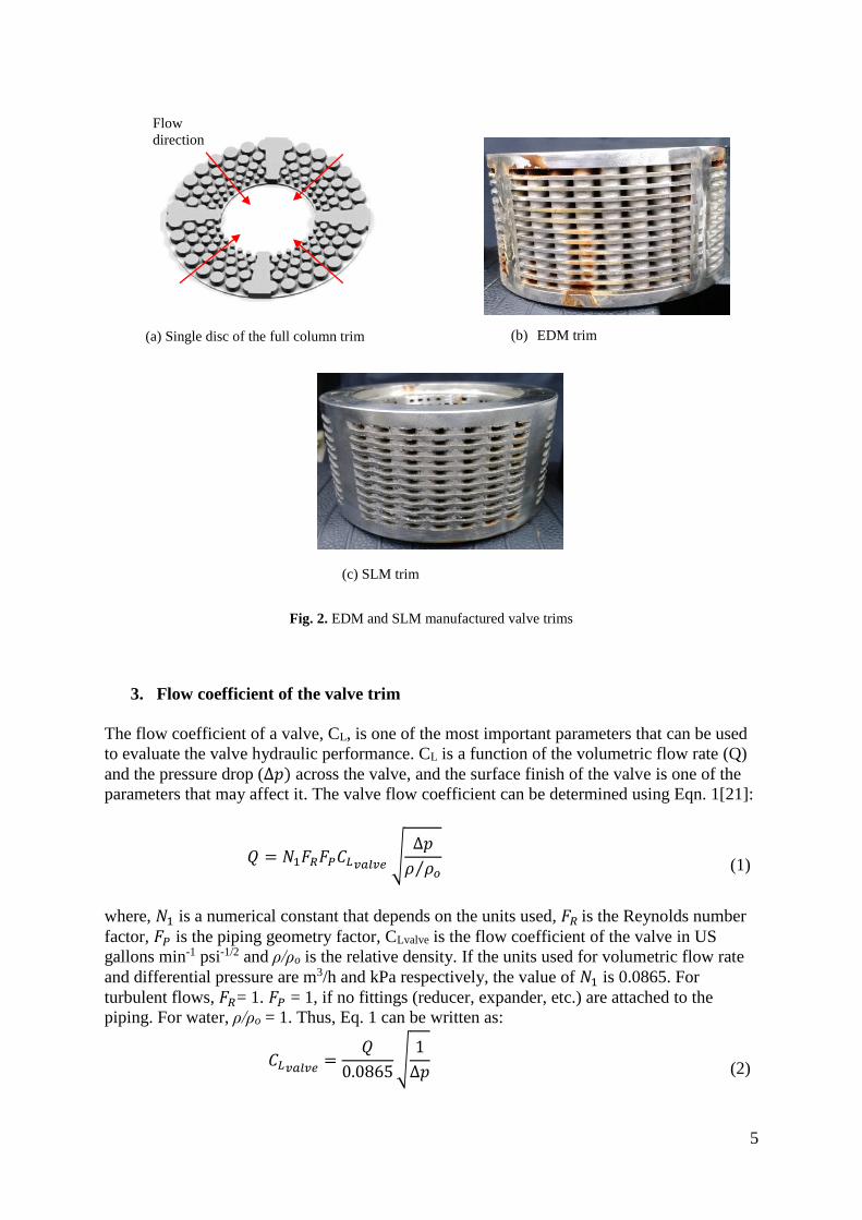
The design of the trim used in this study is quite complex where the fluid flows on well-

designed flow paths on discs that are arranged in a stack. A single disc of the trims is shown

in Fig. 2 (a). As can be seen in the figure, there are five rows of cylinders of varying

diameters on the disc. If the EDM method is used to manufacture such trims, each disc needs

to be manufactured separately and then arranged in a stack and welded together whereas

using the SLM method the whole trim can be manufactured additively. Manufacturing the

trim using SLM also reduced the manufacturing cost by 50%. Figs. 2(b) and 2(c) show the

trims manufactured using the EDM and SLM methods respectively. A Renishaw AM250

machine was used to manufacture the SLM trim. The process parameters for the SLM

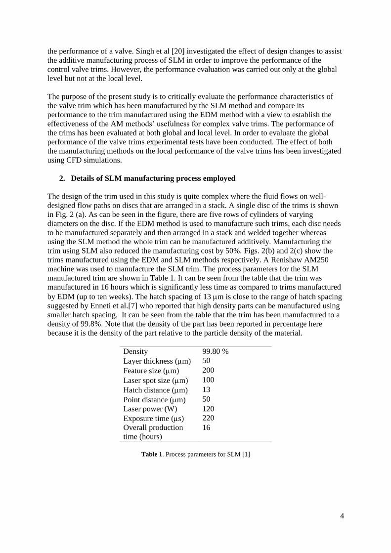
manufactured trim are shown in Table 1. It can be seen from the table that the trim was

manufactured in 16 hours which is significantly less time as compared to trims manufactured

by EDM (up to ten weeks). The hatch spacing of 13 m is close to the range of hatch spacing

suggested by Enneti et al.[7] who reported that high density parts can be manufactured using

smaller hatch spacing. It can be seen from the table that the trim has been manufactured to a

density of 99.8%. Note that the density of the part has been reported in percentage here

because it is the density of the part relative to the particle density of the material.

Density 99.80 %

Layer thickness (m) 50

Feature size (m) 200

Laser spot size (m) 100

Hatch distance (m) 13

Point distance (m) 50

Laser power (W) 120

Exposure time (s) 220

Overall production

time (hours)

16

Table 1. Process parameters for SLM [1]

5

Fig. 2. EDM and SLM manufactured valve trims

3. Flow coefficient of the valve trim

The flow coefficient of a valve, CL, is one of the most important parameters that can be used

to evaluate the valve hydraulic performance. CL is a function of the volumetric flow rate (Q)

and the pressure drop (∆𝑝) across the valve, and the surface finish of the valve is one of the

parameters that may affect it. The valve flow coefficient can be determined using Eqn. 1[21]:

𝑄 = 𝑁1𝐹𝑅𝐹𝑃𝐶𝐿𝑣𝑎𝑙𝑣𝑒 √

∆𝑝

𝜌 𝜌𝑜⁄

(1)

where, 𝑁1 is a numerical constant that depends on the units used, 𝐹𝑅 is the Reynolds number

factor, 𝐹𝑃 is the piping geometry factor, CLvalve is the flow coefficient of the valve in US

gallons min-1 psi-1/2 and ρ/ρo is the relative density. If the units used for volumetric flow rate

and differential pressure are m3/h and kPa respectively, the value of 𝑁1 is 0.0865. For

turbulent flows, 𝐹𝑅= 1. 𝐹𝑃 = 1, if no fittings (reducer, expander, etc.) are attached to the

piping. For water, ρ/ρo = 1. Thus, Eq. 1 can be written as:

𝐶𝐿𝑣𝑎𝑙𝑣𝑒=

𝑄

0.0865√

1

∆𝑝

(2)

(b) EDM trim

(c) SLM trim

Flow

direction

(a) Single disc of the full column trim

6

The valve is composed of the trim, the valve body and the seat, therefore, the overall Δ𝑝

across the valve is the sum of pressure drops across each of these:

Δ𝑝 = ∆𝑝𝑣𝑎𝑙𝑣𝑒 𝑏𝑜𝑑𝑦 + ∆𝑝𝑡𝑟𝑖𝑚 + ∆𝑝𝑠𝑒𝑎𝑡 (3)

As it can be seen from Eq. 2 that the pressure drop is inversely proportional to the square of

the flow coefficient, therefore:

1

𝐶𝐿𝑣𝑎𝑙𝑣𝑒2 =

1

𝐶𝐿𝑣𝑎𝑙𝑣𝑒 𝑏𝑜𝑑𝑦2 +

1

𝐶𝐿𝑡𝑟𝑖𝑚2 +

1

𝐶𝐿𝑠𝑒𝑎𝑡2

(4)

The flow coefficients of the valve body (CLvalve body) and the seat (CLseat) can be calculated as:

𝐶𝐿𝑣𝑎𝑙𝑣𝑒 𝑏𝑜𝑑𝑦= 𝑘1 (

𝐷𝑉𝑎𝑙𝑣𝑒

𝐷𝑆𝑒𝑎𝑡)

2

(5)

and,

𝐶𝐿𝑠𝑒𝑎𝑡= 𝑘2 (

𝐷𝑉𝑎𝑙𝑣𝑒

𝐷𝑆𝑒𝑎𝑡)

2

(6)

where, 𝑘1and 𝑘2 are geometry dependent coefficients of the valve and the seat, and 𝐷𝑉𝑎𝑙𝑣𝑒

and 𝐷𝑆𝑒𝑎𝑡 are the diameters of the valve and seat respectively. Here, the values of CL for the

valve body and the seat are 301.6 and 65 respectively [16].

Therefore, to determine the 𝐶𝑣 value for the trim, Eq. 4 can be transformed into:

1

𝐶𝐿𝑡𝑟𝑖𝑚

= √(1

𝐶𝐿𝑣𝑎𝑙𝑣𝑒2) − (

1

𝐶𝐿𝑣𝑎𝑙𝑣𝑒 𝑏𝑜𝑑𝑦2) − (

1

𝐶𝐿𝑠𝑒𝑎𝑡2) (7)

The trim geometry is designed according to the required CLtrim which is defined by the

process requirements. Therefore, for performance comparison of EDM and SLM trims,

experiments have been conducted to determine the CLvalve. By using the values of the valve

body and seat flow coefficients given above, CLtrim can be calculated using Eqn. 7.

4. Experimental set-up

The flow loop for testing the capacity of the valve trims has been set up according to standard

BS EN 60534-2-3 [21], and test procedure VT-QC-SP503 [22]. The valve used in this study

is a globe valve with inlet and outlet diameter of 100 mm. The valve is attached to a pipe of

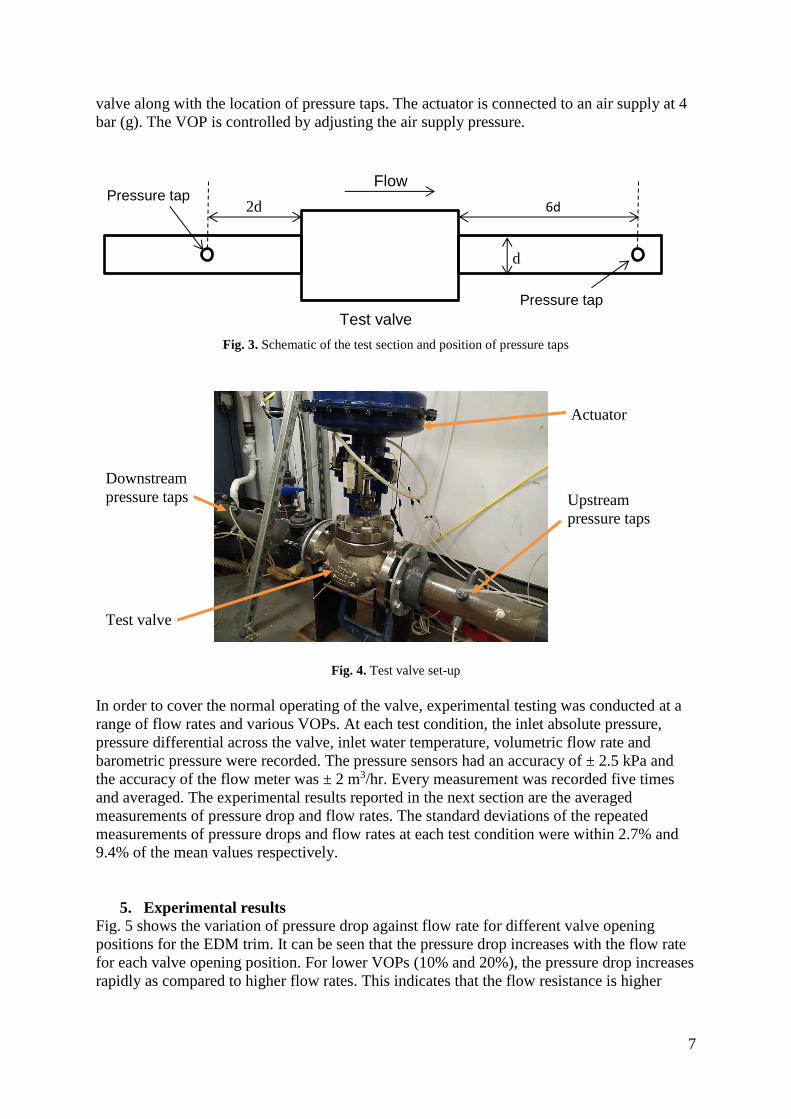
nominal diameter 100 mm in the arrangement shown in Fig. 3. The length of the upstream

pipe is 2 m while the downstream pipe is 1.8 m long. Inlet pressure at the valve is measured

at pressure taps installed at a distance of 200 mm upstream of the valve while the outlet

pressure is measured at pressure taps installed 600 mm downstream of the valve. There are

four pressure taps at the upstream and downstream locations which are installed

circumferentially and spaced equally at both locations. At these locations, average pressure is

measured by the pressure transducers. Water is circulated through the flow loop by a

centrifugal pump. The flow rate is measured using a turbine flow meter. The data from the

turbine flow meter and the pressure transducers is collected via Omega USB-4718 data

acquisition module. The temperature of the test fluid is measured using a thermocouple which

is installed within the water storage tank. Fig. 4 shows the pneumatically actuated control

7

valve along with the location of pressure taps. The actuator is connected to an air supply at 4

bar (g). The VOP is controlled by adjusting the air supply pressure.

Fig. 3. Schematic of the test section and position of pressure taps

Fig. 4. Test valve set-up

In order to cover the normal operating of the valve, experimental testing was conducted at a

range of flow rates and various VOPs. At each test condition, the inlet absolute pressure,

pressure differential across the valve, inlet water temperature, volumetric flow rate and

barometric pressure were recorded. The pressure sensors had an accuracy of ± 2.5 kPa and

the accuracy of the flow meter was ± 2 m3/hr. Every measurement was recorded five times

and averaged. The experimental results reported in the next section are the averaged

measurements of pressure drop and flow rates. The standard deviations of the repeated

measurements of pressure drops and flow rates at each test condition were within 2.7% and

9.4% of the mean values respectively.

5. Experimental results

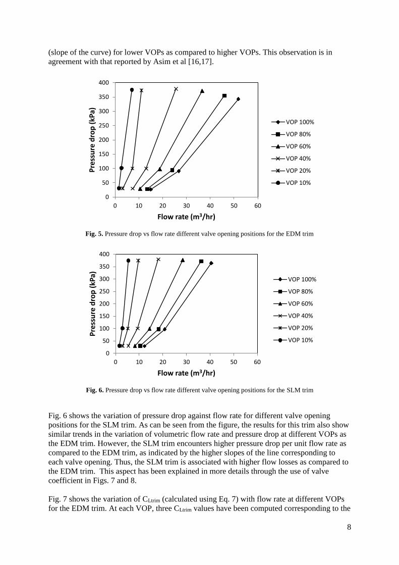
Fig. 5 shows the variation of pressure drop against flow rate for different valve opening

positions for the EDM trim. It can be seen that the pressure drop increases with the flow rate

for each valve opening position. For lower VOPs (10% and 20%), the pressure drop increases

rapidly as compared to higher flow rates. This indicates that the flow resistance is higher

d

Flow

Pressure tap

Pressure tap 2d 6d

Test valve

Downstream

pressure taps Upstream

pressure taps

Test valve

Actuator

8

(slope of the curve) for lower VOPs as compared to higher VOPs. This observation is in

agreement with that reported by Asim et al [16,17].

Fig. 5. Pressure drop vs flow rate different valve opening positions for the EDM trim

Fig. 6. Pressure drop vs flow rate different valve opening positions for the SLM trim

Fig. 6 shows the variation of pressure drop against flow rate for different valve opening

positions for the SLM trim. As can be seen from the figure, the results for this trim also show

similar trends in the variation of volumetric flow rate and pressure drop at different VOPs as

the EDM trim. However, the SLM trim encounters higher pressure drop per unit flow rate as

compared to the EDM trim, as indicated by the higher slopes of the line corresponding to

each valve opening. Thus, the SLM trim is associated with higher flow losses as compared to

the EDM trim. This aspect has been explained in more details through the use of valve

coefficient in Figs. 7 and 8.

Fig. 7 shows the variation of CLtrim (calculated using Eq. 7) with flow rate at different VOPs

for the EDM trim. At each VOP, three CLtrim values have been computed corresponding to the

0

50

100

150

200

250

300

350

400

0 10 20 30 40 50 60

Pre

ssu

re d

rop

(kP

a)

Flow rate (m3/hr)

VOP 100%

VOP 80%

VOP 60%

VOP 40%

VOP 20%

VOP 10%

0

50

100

150

200

250

300

350

400

0 10 20 30 40 50 60

Pre

ssu

re d

rop

(kP

a)

Flow rate (m3/hr)

VOP 100%

VOP 80%

VOP 60%

VOP 40%

VOP 20%

VOP 10%

9

three flow rates and pressure drops that were shown in Fig. 5. It can be seen from the figure

that CLtrim remains nearly constant for each valve opening position. This is expected because

CLtrim is dependent on the VOP, and not the flow conditions. These results are consistent with

the findings of Asim et al [15,16] and Oliveira [18]. It can also be seen from the figure that

CLtrim increases linearly with increase in VOP. Fig. 8 shows the variation of CLtrim with flow

rate at various VOPs for the SLM trim. Again, it can be seen from the figure that CLtrim

remains nearly constant for each VOP and increases linearly with increase in VOP, similar to

the EDM trim. At 100 % VOP, the average value of CLtrim for the EDM trim is 37.52 while it

is 26.58 for the SLM trim, which is a 29% drop in the performance.

Fig. 7. Variation of CLtrim with flow rate at various valve opening positions – EDM trim

Fig. 8. Variation of CLtrim with flow rate at various valve opening positions – SLM trim

0

5

10

15

20

25

30

35

40

45

0 10 20 30 40 50 60

CLt

rim

Flow rate (m3/hr)

VOP 100%

VOP 80%

VOP 60%

VOP 40%

VOP 20%

VOP 10%

0

5

10

15

20

25

30

0 10 20 30 40 50

CLt

rim

Flow rate (m3/hr)

VOP 100%

VOP 80%

VOP 60%

VOP 40%

VOP 20%

VOP 10%

10

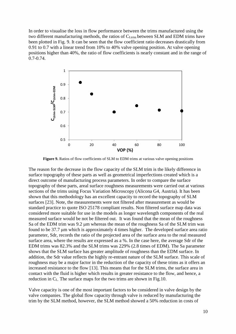
In order to visualise the loss in flow performance between the trims manufactured using the

two different manufacturing methods, the ratios of CLtrim between SLM and EDM trims have

been plotted in Fig. 9. It can be seen that the flow coefficient ratio decreases drastically from

0.91 to 0.7 with a linear trend from 10% to 40% valve opening position. At valve opening

positions higher than 40%, the ratio of flow coefficients is nearly constant and in the range of

0.7-0.74.

Figure 9. Ratios of flow coefficients of SLM to EDM trims at various valve opening positions

The reason for the decrease in the flow capacity of the SLM trim is the likely difference in

surface topography of these parts as well as geometrical imperfections created which is a

direct outcome of manufacturing process parameters. In order to compare the surface

topography of these parts, areal surface roughness measurements were carried out at various

sections of the trims using Focus Variation Microscopy (Alicona G4, Austria). It has been

shown that this methodology has an excellent capacity to record the topography of SLM

surfaces [23]. Note, the measurements were not filtered after measurement as would be

standard practice to quote ISO 25178 compliant results. Non filtered surface map data was

considered more suitable for use in the models as longer wavelength components of the real

measured surface would be not be filtered out. It was found that the mean of the roughness

Sa of the EDM trim was 9.2 μm whereas the mean of the roughness Sa of the SLM trim was

found to be 37.7 μm which is approximately 4 times higher. The developed surface area ratio

parameter, Sdr, records the ratio of the projected area of the surface area to the real measured

surface area, where the results are expressed as a %. In the case here, the average Sdr of the

EDM trims was 82.3% and the SLM trims was 229% (2.8 times of EDM). The Sa parameter

shows that the SLM surface has greater amplitude of roughness than the EDM surface. In

addition, the Sdr value reflects the highly re-entrant nature of the SLM surface. This scale of

roughness may be a major factor in the reduction of the capacity of these trims as it offers an

increased resistance to the flow [13]. This means that for the SLM trims, the surface area in

contact with the fluid is higher which results in greater resistance to the flow, and hence, a

reduction in CL. The surface maps for the two trims are shown in Fig.10.

Valve capacity is one of the most important factors to be considered in valve design by the

valve companies. The global flow capacity through valve is reduced by manufacturing the

trim by the SLM method, however, the SLM method showed a 50% reduction in costs of

0.5

0.6

0.7

0.8

0.9

1

0 20 40 60 80 100

CLt

rim

-SLM

/CLt

rim

-ED

M

VOP (%)

11

manufacture and significant reduction in manufacturing lead time. The estimation of effects

of local roughness variations on flow performance using experimental means is very difficult

hence the possibility of using a well validated numerical scheme for this purpose has been

explored in the next section.

Figure 10. Areal surface maps of a) EDM surface b) SLM surface, maps plotted on same scale

6. CFD modelling of the control valve

In the previous section, the global flow parameters of the valves manufactured by both the

manufacturing methods have been determined by experimental methods. The experimental

methods currently can only provide information on the global performance parameters and

have severe limitations in providing local flow field information. During the operation of

valves, various problems such as cavitation and erosion can develop, which are local

phenomena and therefore, it is important to investigate the local flow parameters of the

valves which could be utilised to optimise the performance characteristics of the valve trims.

The investigation of local flow parameters can also provide detailed information on how the

change in the surface finish affects the flow field within the discs of the valve trim locally

which affects the overall CL. Therefore, in order to evaluate the effect of the manufacturing

method on the local performance of the valve trims, numerical simulations have been

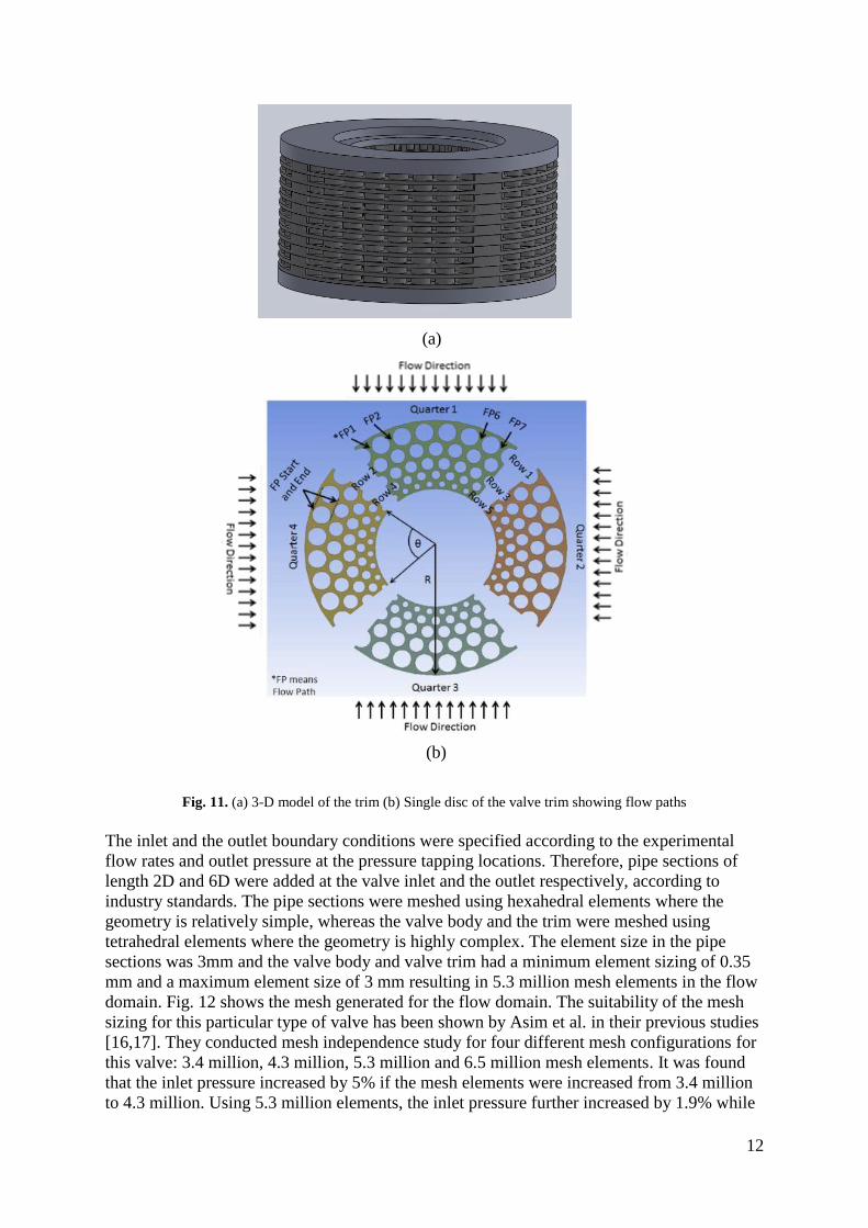
conducted. The three-dimensional model of the valve trim used in these simulations is shown

in Fig. 11. There are 11 discs in the trim stack and the flow direction within the discs is from

the outer diameter towards the inner diameter, i.e., from row 1 to row 5 as shown in Fig.

11(a). Each disc is made up of four identical quarters. In each quarter, there are different flow

paths in between the cylinders where fluid can flow. There are 7 flow paths on rows 1, 3 and

5 whereas there are 8 flow paths on rows 2 and 4 as shown in Fig. 11(b).

(a) (b)

12

Fig. 11. (a) 3-D model of the trim (b) Single disc of the valve trim showing flow paths

The inlet and the outlet boundary conditions were specified according to the experimental

flow rates and outlet pressure at the pressure tapping locations. Therefore, pipe sections of

length 2D and 6D were added at the valve inlet and the outlet respectively, according to

industry standards. The pipe sections were meshed using hexahedral elements where the

geometry is relatively simple, whereas the valve body and the trim were meshed using

tetrahedral elements where the geometry is highly complex. The element size in the pipe

sections was 3mm and the valve body and valve trim had a minimum element sizing of 0.35

mm and a maximum element size of 3 mm resulting in 5.3 million mesh elements in the flow

domain. Fig. 12 shows the mesh generated for the flow domain. The suitability of the mesh

sizing for this particular type of valve has been shown by Asim et al. in their previous studies

[16,17]. They conducted mesh independence study for four different mesh configurations for

this valve: 3.4 million, 4.3 million, 5.3 million and 6.5 million mesh elements. It was found

that the inlet pressure increased by 5% if the mesh elements were increased from 3.4 million

to 4.3 million. Using 5.3 million elements, the inlet pressure further increased by 1.9% while

(a)

(b)

13

increasing the mesh elements to 6.5 million, the inlet pressure decreased by 0.9%. The mesh

with 5.3 million elements was chosen because the difference in the inlet pressure was less

than 1% as compared to the mesh with 6.5 million elements [16,17]. ANSYS Fluent 17.0 has

been used to conduct the numerical flow simulations. The turbulence model employed is a

two equation Shear Stress Transport (SST) k-ω model because it has been shown to be

effective in modelling the severe velocity gradients accurately in control valve applications

[24–27].

(a)

(b)

Fig. 12. Mesh in (a) the valve (b) the trim

The effect of the surface roughness of the trims was modelled by using the modified law-of-

the-wall for roughness [28] which is defined as:

𝑢𝑝𝑢∗

𝜏𝑤 𝜌⁄=

1

𝐾ln (𝐸

𝜌𝑢∗𝑦𝑝

𝜇) − ∆𝐵 (7)

where, 𝑢𝑝 is the fluid mean velocity at the wall-adjacent cell centroid, 𝑢∗ is the friction

velocity, 𝑦𝑝 is the distance from the wall to the wall-adjacent cell centroid, 𝜏𝑤 is the wall

shear stress, 𝐾 = 0.4187 is the von Karman constant, 𝐸 = 9.793 is an empirical constant and 𝜇

14

is the dynamic viscosity of the fluid. The friction velocity is related to a constant 𝐶𝜇 and the

turbulent kinetic energy (𝑘) by the following equation:

𝑢∗ = 𝐶𝜇0.25𝑘0.5 (8)

∆𝐵 is related to 𝐾𝑠+ (non-dimensional roughness height) which is defined as:

𝐾𝑠+ =

𝜌𝐾𝑠𝑢∗

𝜇 (9)

where, 𝐾𝑠 is the physical roughness value.

For hydrodynamically smooth regime (𝐾𝑠+ ≤ 2.25):

∆𝐵 = 0 (10)

For the transitional regime (2.25 ≤ 𝐾𝑠+ ≤ 90):

∆𝐵 =1

𝐾ln [

𝐾𝑠+ − 2.25

87.75+ 𝐶𝑠𝐾𝑠

+] × sin[0.4258(ln 𝐾𝑠+ − 0.811)] (11)

where, 𝐶𝑠 is a roughness constant which depends on the type of roughness.

In the fully rough regime (𝐾𝑠+ > 90):

∆𝐵 =1

𝐾ln(1 + 𝐶𝑠𝐾𝑠

+) (12)

In the simulations conducted for this paper, a roughness height (𝐾𝑠) of 500 microns and 1000

microns was specified for the EDM and SLM trims respectively. These 𝐾𝑠 values have been

chosen to match the global CL results with experiments and to take into account that several

flow paths that were found to be completely blocked on the SLM trim. The roughness

constant (𝐶𝑠) was specified as 1 to represent the non-uniform roughness.

In order to determine the accuracy of the numerical modelling, CFD results have been

verified against the experimental results by comparing the CLtrim values as shown in Table 2.

The simulations for both trims were run at 100 % VOP. It can be seen in the table that there is

a difference of only 3.27% and 1.8% in the CLtrim values for the EDM and SLM trims

respectively. Therefore, the CFD results show a close agreement with the experimental

results.

Trim Experimental

CLtrim

CFD predicted

CLtrim

% Difference

EDM 37.52 36.29 -3.27

SLM 26.58 27.06 +1.8

Table 2. Verification of CFD results

15

7. Local performance analysis of the EDM and SLM trims

In order to compare the performance of the two trims on the local level, a detailed

investigation was conducted on local flow coefficients within the trims at different flow paths

within different rows of cylinders on the discs as well as the variation of pressure and

velocity within the top disc in the trims at the 100 % valve opening position. This analysis is

shown on a quarter of the disc as the other quarters exhibit similar behaviour.

7.1 Local flow coefficients

In order to evaluate the difference in performance of the valve trims at local level, flow

capacities were calculated at all the flow paths on a quarter of the top disc of the valve trims.

The local flow coefficient of a flow path was calculated using the pressure drop and the flow

rate across each flow path using Eqn. 2. Fig. 13 shows the location of these flow paths on a

quarter of the trim disc. As can be seen from the figure, there are seven flow paths in rows 1,

3 and 5 whereas there are eight flow paths. The start and end of each flow path is considered

to be at the entry and exit of each row of cylinders. Table 3 shows normalised local flow

coefficients of all flow paths at each row of cylinders on the EDM trim while Table 4 shows

normalised local flow coefficients of all flow paths of the SLM trim. The coefficients have

been normalised by the average of flow path flow coefficients for each row. The tables show

that the normalised local flow coefficients remain nearly constant (close to 1) at different

flow paths of first, third and fifth rows because the all the flow paths are similar. At second

and fourth rows, the normalised local flow coefficients are nearly 0.5 in flow paths 1 and 8

whereas they are in the range of 1.1-1.2 in flow paths 2-7. This is because of the difference

in the geometry of flow paths 1 and 2 as compared to other flow paths in rows 2 and 4.

Fig. 13. Flow paths between cylinders on a quarter of the trim disc (FP = flow path)

It can be seen from Table 3 that, for the EDM trim, the highest flow coefficient is observed to

at row 5 while row 3 has the lowest flow coefficient. In the direction of flow, there is a

reduction of 8 % in the average local flow coefficient from row 1 to 2, a reduction of 2 %

FP start

FP end

16

from row 2 to 3 whereas it increases by 2.8 % from row 3 to 4 and by 36.5 % from row 4 to

5. From Table 4, it can be seen that for the SLM trim, the highest flow coefficient is still

observed at row 5 but the lowest flow coefficient is seen at row 4. The normalised local flow

coefficient in the SLM trim decreases from row 1 to 2 by 8.7 %, from row 2 to 3 by 2.5 %,

from row 3 to 4 by 1.9 % whereas it increases from row 4 to 5 by 3.3 %.

Flow path

CL- Flow path / Average CL-Row

Row 1 Row 2 Row 3 Row 4 Row 5

1 1.007 0.502 1.004 0.514 1.006 2 1.007 1.174 1.008 1.192 1.003

3 0.985 1.178 1.004 1.137 0.994 4 0.993 1.190 0.992 1.176 0.989 5 1.018 1.126 0.984 1.137 0.971 6 1.011 1.134 0.984 1.161 0.994 7 0.989 1.166 1.012 1.141 1.049 8

0.514

0.545

Average CL-Row

0.275 0.253 0.248 0.255 0.348

Table 3. Local flow coefficients of different flow paths of a quarter of the top disc of the EDM trim

Flow path

CL-Flow path/Average CL –Row

Row 1 Row 2 Row 3 Row 4 Row 5

1 0.997 0.506 1.006 0.521 1.020 2 0.993 1.153 1.000 1.162 0.996 3 1.001 1.167 1.001 1.172 0.989 4 1.008 1.175 0.999 1.160 0.987 5 1.001 1.162 0.986 1.146 0.988 6 0.994 1.164 0.997 1.151 0.993 7 1.006 1.160 1.009 1.160 1.027

8 0.512 0.528

Average CL-Row

0.267 0.244 0.237 0.233 0.311

Table 4. Local flow coefficients of different flow paths of a quarter of the top disc of the SLM trim

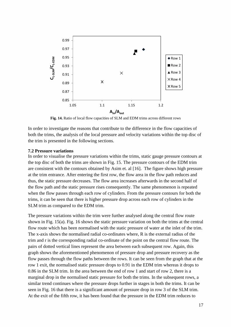
Comparing the local flow coefficients of the rows in both the trims shows that the local flow

coefficients of all the rows are lower in the SLM trim. The decrease in the flow coefficient in

the SLM trim for rows 1 to 5 is 3%, 3.7%, 4.2%, 8.6% and 10.6% respectively. The decrease

in the flow capacity of each row contributes to the overall drop in CL for the trim

manufactured by the SLM method. The decrease in the flow coefficients is depicted in the

form of ratios of the flow capacities of SLM and EDM across different rows in Fig. 14. In

this graph, the ratio of flow coefficients ratio is plotted against Ain/Aout, where Ain is the area

at the inlet and Aout is the area at the outlet of the flow paths at each row. The graph shows

that decrease in the flow coefficient ratios increase with increase in Ain/Aout. The flow

coefficient ratio is highest in row 1 and minimum in row 5.

17

Fig. 14. Ratio of local flow capacities of SLM and EDM trims across different rows

In order to investigate the reasons that contribute to the difference in the flow capacities of

both the trims, the analysis of the local pressure and velocity variations within the top disc of

the trim is presented in the following sections.

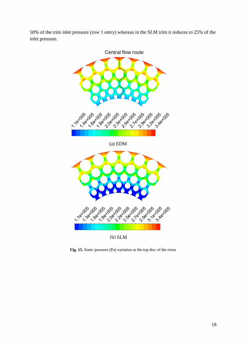
7.2 Pressure variations

In order to visualise the pressure variations within the trims, static gauge pressure contours at

the top disc of both the trims are shown in Fig. 15. The pressure contours of the EDM trim

are consistent with the contours obtained by Asim et. al [16]. The figure shows high pressure

at the trim entrance. After entering the first row, the flow area in the flow path reduces and

thus, the static pressure decreases. The flow area increases afterwards in the second half of

the flow path and the static pressure rises consequently. The same phenomenon is repeated

when the flow passes through each row of cylinders. From the pressure contours for both the

trims, it can be seen that there is higher pressure drop across each row of cylinders in the

SLM trim as compared to the EDM trim.

The pressure variations within the trim were further analysed along the central flow route

shown in Fig. 15(a). Fig. 16 shows the static pressure variation on both the trims at the central

flow route which has been normalised with the static pressure of water at the inlet of the trim.

The x-axis shows the normalised radial co-ordinates where, R is the external radius of the

trim and r is the corresponding radial co-ordinate of the point on the central flow route. The

pairs of dotted vertical lines represent the area between each subsequent row. Again, this

graph shows the aforementioned phenomenon of pressure drop and pressure recovery as the

flow passes through the flow paths between the rows. It can be seen from the graph that at the

row 1 exit, the normalised static pressure drops to 0.91 in the EDM trim whereas it drops to

0.86 in the SLM trim. In the area between the end of row 1 and start of row 2, there is a

marginal drop in the normalised static pressure for both the trims. In the subsequent rows, a

similar trend continues where the pressure drops further in stages in both the trims. It can be

seen in Fig. 16 that there is a significant amount of pressure drop in row 3 of the SLM trim.

At the exit of the fifth row, it has been found that the pressure in the EDM trim reduces to

0.85

0.87

0.89

0.91

0.93

0.95

0.97

0.99

1.05 1.1 1.15 1.2

CL-

SLM

/CL-

EDM

Ain/Aout

Row 1

Row 2

Row 3

Row 4

Row 5

18

50% of the trim inlet pressure (row 1 entry) whereas in the SLM trim it reduces to 25% of the

inlet pressure.

Fig. 15. Static pressure (Pa) variation at the top disc of the trims

Central flow route

(b) SLM

(a) EDM

19

Fig. 16. Normalised static pressure variations within the top disc of the trims along the central flow route

The ratio of normalised static pressure variation of SLM and EDM trims along the central flow

path has been presented in Fig. 17. The figure also shows that the pressure ratio decreases at a

significantly higher rate in rows 3, 4 and 5 than the first two rows. At the exit from the trim at

the end of row 5, the normalised static pressure in SLM trim is half of that in the EDM trim.

Fig. 17. Variations of normalised static pressure ratio between SLM and EDM trims along the central flow route

In order to compare the pressure drop across various rows of the disc, normalised differential

pressure across each row along the central flow route is plotted in Fig. 18. It can be seen that

the pressure drop is higher at each row in the SLM trim as outlined previously. For both the

trims, the pressure drop is slightly lower in the second row as compared to the first row. The

20

decreasing trend continues in row 3 for the EDM trim, however, it increases in the fourth row

and then decreases again in the fifth row. On the other hand, for the SLM trim, the pressure

drop in the third row is the highest after which it shows a decreasing trend. It was found that

row 3 of the SLM trim contributes to 26% of the overall pressure drop across the top disc of

the trim.

Fig. 18. Normalised differential static pressure across different rows at the central flow route within the top disc

of the trims

Fig. 19 shows the ratio of normalised differential pressures of SLM and EDM trims at each

row plotted against Ain/Aout. The differential pressure ratios in rows 1-5 are 1.76, 1.78, 4.22,

2.18 and 2.82 respectively, giving an average of 2.55 across all rows. It can be seen in the

figure that the normalised differential pressure ratio decreases with increase in Ain/Aout,

except row 3, where it is the highest. Abnormal flow behaviour at row 3 of this kind of trim

was also reported by Asim et al. [29] while investigating the pressure losses per unit radial

distance. The next highest point in the graph is at row 5. The pressure drop across the flow

paths is the combined effect of geometrical features of the flow paths as well as the surface

roughness. Previous papers by Asim et al. [16,17] have discussed the effect of the

geometrical features on the pressure drop across the flow paths and they showed how change

in the geometrical features affected the pressure drop across each flow path for EDM

manufactured trims. In the present paper, the geometrical features of both the trims are

similar to those used by Asim et al., therefore, Figs. 16-19 show how the variation of surface

roughness affects the pressure drop across each flow path.

21

Figure 19. Normalised differential static pressure ratio of SLM and EDM across different rows within the top

disc

7.3 Velocity variations

After analysing the pressure variations for both the trims, velocity variations within the trims

at the top disc are presented in this section. Fig. 20 shows the flow velocity magnitude

contours at a quarter of the top disc of both the trims. It can be seen from the figure that after

entry in each row of the trim, the flow velocity increases as it passes the narrow area between

the cylinders in a row and then decreases with increase in the flow area towards the exit of

each row. The maximum velocity of the fluid in the EDM trim along the central flow path is

each row is 12 m/s (Row 1), 11.5 m/s (Row 2), 12.7 m/s (Row 3), 11 m/s (Row 4) and 9.9

m/s (Row 5), whereas in the SLM trim, the maximum flow velocity in each row is 8.9 m/s

(Row 1), 8.93 m/s (Row 2), 10.3 m/s (Row 3), 9.3 m/s (Row 4) and 6.8 m/s (Row 5). Thus, it

can be seen that the flow velocities are higher in the EDM trim as compared to the SLM trim

due to the reason that in the SLM trim, the resistance to flow is greater due to its greater

surface roughness. These simulations were conducted for a similar pressure drop which

resulted in lower flow rate with the SLM trim case which results in the lower flow velocities

in the flow paths. The reduction in maximum flow velocities in the SLM trim from rows 1-5

is 11.2%, 11.2%, 9.7%, 10.8% and 14.7% respectively.

1

1.5

2

2.5

3

3.5

4

4.5

1.05 1.1 1.15 1.2

Ain/Aout

Row 1

Row 2

Row 3

Row 4

Row 5

𝜟𝐩

𝐩𝐢𝐧

𝐥𝐞𝐭

𝑺𝑳

𝑴

𝜟𝐩

𝐩𝐢𝐧

𝐥𝐞𝐭

𝑬𝑫

𝑴

22

Fig. 20. Velocity (m/s) variation within the top disc of the trims

Fig. 21. Arcs in the middle of each row for velocity profile extraction

Flow velocity was extracted at an arc passing through each row of the discs as shown in Fig.

21 for analysing the flow velocity further. The normalised velocity profiles at each row are

presented in Figs. 22 and 23. Due to the reason that rows 1, 3 and 5 have seven flow paths

(a) EDM

(b) SLM

23

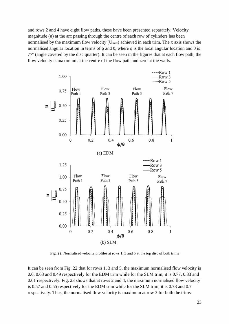
and rows 2 and 4 have eight flow paths, these have been presented separately. Velocity

magnitude (u) at the arc passing through the centre of each row of cylinders has been

normalised by the maximum flow velocity (Umax) achieved in each trim. The x axis shows the

normalised angular location in terms of ϕ and θ, where ϕ is the local angular location and θ is

77o (angle covered by the disc quarter). It can be seen in the figures that at each flow path, the

flow velocity is maximum at the centre of the flow path and zero at the walls.

Fig. 22. Normalised velocity profiles at rows 1, 3 and 5 at the top disc of both trims

It can be seen from Fig. 22 that for rows 1, 3 and 5, the maximum normalised flow velocity is

0.6, 0.63 and 0.49 respectively for the EDM trim while for the SLM trim, it is 0.77, 0.83 and

0.61 respectively. Fig. 23 shows that at rows 2 and 4, the maximum normalised flow velocity

is 0.57 and 0.55 respectively for the EDM trim while for the SLM trim, it is 0.73 and 0.7

respectively. Thus, the normalised flow velocity is maximum at row 3 for both the trims

(a) EDM

(b) SLM

24

because row 3 has the smallest available flow area. In contrast, the normalised flow velocity

is minimum at row 5 because it has the maximum flow area. The flow velocity variation

patterns in different flow paths within each row are similar except first and last flow paths of

row 2 and 4 because of their different geometry as compared to other flow paths.

Fig. 23. Normalised velocity profiles at rows 2 and 4 at the top disc of both trims

(a) EDM

(b) SLM

25

Figure 24. Normalised velocity profiles in each row along the central flow path for both trims

Row 1

Row 5

Row 4

Row 3

Row 2

26

The normalised velocity profile in the central flow paths in each row is depicted in Fig. 24 for

both the EDM and SLM trims, where, URow is the maximum velocity in the row. It can be

seen that the velocity profile in the SLM trim becomes flatter due to the effect of the

increased surface roughness. For the EDM trim, the velocity profile is the peaky in the first

two rows and it becomes flatter as it goes along the flow paths in subsequent rows on the

disc. The velocity profile in row 5 of both trims shows two peaks and a dip in the middle. The

location of these high velocity regions in row 5 can be seen in Fig. 20 along the sides of the

cylinders in row 5. Furthermore, the gradient of velocity change with increasing distance

from the wall is greater for the SLM trim as comparted to the EDM trim.

7.4 Boundary shear

It has been shown in the previous sections that the performance of the valve trim decreased

with the change of surface finish/roughness. The reason for the drop in performance is

because of the increased boundary shear due to the increased surface roughness. In order to

present the effect of roughness, wall shear stress has been calculated for each flow path along

the central flow route. Fig. 25 shows the average wall shear stress at the flow paths in each

row in both the trims. It can be seen that the wall shear stress is higher in all the rows in the

SLM trim as compared to the EDM trim because of the higher surface roughness. The highest

wall shear stress occurs at row 4 whereas the lowest wall shear stress occurs at row 1 for both

the trims. On average, the wall shear stress in the SLM trim is 1.9 times higher than the EDM

trim. The trend in the wall shear stress is similar for both the trims across different rows.

Fig. 25. Wall shear stress along the central flow path at different rows of EDM and SLM trims

The ratios of wall shear stress between the SLM and EDM trims at each row are plotted in

Fig. 26. The wall shear stress ratio can be seen to vary from 1.85 to 1.99 between different

rows of the trims and it is seen to be maximum at row 3. The wall shear stress ratio is

minimum at row 1 which then increases in row 2 and 3 and then drops in rows 4 and 5. This

explains the reason for the highest pressure drop occurring in row 3 of the SLM trim.

0

500

1,000

1,500

2,000

2,500

3,000

3,500

4,000

1 2 3 4 5

t wal

l(P

a)

Row number

EDM

SLM

27

Figure 26. Wall shear stress ratio of SLM to EDM trim at each row along the central flow path

Thus, the analysis of results from CFD simulations have shown how the change in surface

roughness due to manufacturing method has changed the local flow parameters, such as

pressure, velocity and wall shear stress on the flow paths of the trims. The Sdr parameter for

the SLM trim was 2.8 times and the Sa was four times of that for the EDM trim. Increase in

surface roughness lead to an increase in the wall shear stress of 1.9 times on average across

all the rows of the trim. The maximum pressure drop has been observed to occur at row 3 of

the SLM trim which is due to the highest increase in the wall shear stress occurring at row 3

as seen in Fig. 26. However, the maximum decrease in the local flow coefficient has been

noticed at row 5 where the differential pressure drop ratio between the SLM and EDM trims

is the second highest and the decrease in maximum velocity is the highest. Therefore, it has

been seen that rows 3 and 5 are the highest contributors in the decrease in the performance of

the trim manufactured using the SLM method.

The surface roughness of AM parts is highly re-entrant in nature and it is probable that

conventional line of sight measured roughness parameters underestimate the scale of

roughness and certainly would underestimate the real surface area [30]. Enabling the re-

entrant nature to be included in model could enhance the accuracy of the modelling.

The above results indicate that although the additive manufacturing methods offer significant

advantages in the manufacturing processes, the effectiveness of products manufactured needs

to be carefully investigated. This is particularly true for flow handling equipment as it may

have both local as well as global effects.

8. Conclusion

The traditional method of EDM requires a significant amount of time and cost to manufacture

a complex geometry multi-stage disc stack trim. Therefore, in order to reduce costs of

manufacturing, a valve trim was manufactured by employing the additive manufacturing

method of SLM and its performance was tested. The experimental testing of the trim showed

performance of the trim was reduced as compared to the EDM manufactured trim due to the

1.84

1.86

1.88

1.90

1.92

1.94

1.96

1.98

2.00

1 2 3 4 5

t wall

-SL

M/t

wall

-ED

M

Row number

28

higher surface roughness of the SLM manufactured valve trim. Local performance analysis

using CFD showed that the rows 3 and 5 of the SLM trim to be the highest contributors to the

decrease in the flow capacity of the trim because the pressure drop ratios are higher in these

rows as compared to the EDM trim. The increase in pressure drop in the SLM trim is due to

the wall shear stress increase in the SLM trim because of the higher surface roughness. On

average, the wall shear stress in the SLM trim has been found to be 1.9 times higher than the

EDM trim. Despite the shortcomings in performance, the SLM trim was manufactured in a

considerably shorter time and a cost reduction of 50% was achieved as compared with the

trim manufactured by EDM. Finishing processes have been developed that can reduce the

roughness of complex AM parts however their effectiveness in reducing roughness in

complex parts and the effect on changing the geometry of the trim elements needs further

study [31]. Consequently, the additive manufacturing method of SLM with additional

finishing is possibly still viable commercially.

References

[1] M. Charlton, Cost effective manufacturing and optimal design of X-stream trims for

severe service control valves, MSc Thesis, University of Huddersfield, 2014.

[2] M. Charlton, R. Mishra, T. Asim, The effect of manufacturing method induced

roughness on severe service control valve performance, in: Proc. 6th Int. 43rd Natl.

Conf. Fluid Mech. Fluid Power, 2016.

[3] M.K. Thompson, G. Moroni, T. Vaneker, G. Fadel, R.I. Campbell, I. Gibson, A.

Bernard, J. Schulz, P. Graf, B. Ahuja, F. Martina, Design for Additive Manufacturing:

Trends, opportunities, considerations, and constraints, CIRP Ann. 65 (2016) 737–760.

doi:10.1016/j.cirp.2016.05.004.

[4] D. Herzog, V. Seyda, E. Wycisk, C. Emmelmann, Additive manufacturing of metals,

Acta Mater. 117 (2016) 371–392. doi:10.1016/j.actamat.2016.07.019.

[5] Q.B. Nguyen, D.N. Luu, S.M.L. Nai, Z. Zhu, Z. Chen, J. Wei, The role of powder layer

thickness on the quality of SLM printed parts, Arch. Civ. Mech. Eng. 18 (2018) 948–

955. doi:10.1016/J.ACME.2018.01.015.

[6] S. Tsopanos, Micro heat exchangers by selective laser melting, PhD thesis, University

of Liverpool (2008).

[7] R.K. Enneti, R. Morgan, S. V. Atre, Effect of process parameters on the Selective Laser

Melting (SLM) of tungsten, Int. J. Refract. Met. Hard Mater. 71 (2018) 315–319.

doi:10.1016/J.IJRMHM.2017.11.035.

[8] P. Hanzl, M. Zetek, T. Bakša, T. Kroupa, The Influence of Processing Parameters on the

Mechanical Properties of SLM Parts, Procedia Eng. 100 (2015) 1405–1413.

doi:10.1016/J.PROENG.2015.01.510.

[9] K. Osakada, M. Shiomi, Flexible manufacturing of metallic products by selective laser

melting of powder, Int. J. Mach. Tools Manuf. 46 (2006) 1188–1193.

doi:10.1016/J.IJMACHTOOLS.2006.01.024.

[10] B.N. Turner, S.A. Gold, A review of melt extrusion additive manufacturing processes:

II. Materials, dimensional accuracy, and surface roughness, Rapid Prototyp. J. 21 (2015)

250–261. doi:10.1108/RPJ-02-2013-0017.

[11] S. Thamizhmanii, S. Saparudin, S. Hasan, Analyses of surface roughness by turning

process using Taguchi method, J. Achiev. Mater. Manuf. Eng. 20 (2007) 503–505.

doi:10.1007/s00170-007-1147-0.

29

[12] L. Blunt, X. Jiang, Advanced techniques for assessment of surface topography, Kogan

Page Science, 2003.

[13] J.B. Taylor, A.L. Carrano, S.G. Kandlikar, Characterization of the effect of surface

roughness and texture on fluid flow—past, present, and future, Int. J. Therm. Sci. 45

(2006) 962–968. doi:10.1016/j.ijthermalsci.2006.01.004.

[14] J. Green, R. Mishra, M. Charlton, R. Owen, Validation of CFD predictions using process

data obtained from flow through an industrial control valve, J. Phys. Conf. Ser. 364

(2012) 012074. doi:10.1088/1742-6596/364/1/012074.

[15] T. Asim, R. Mishra, M. Charlton, C. Oliveira, Capacity Testing and Local Flow Analysis

of a Geometrically Complex Trim Installed within a Commercial Control Valve, in: Int.

Conf. Jets, Wakes Separated Flows, Stockholm, Sweden, 2015.

[16] T. Asim, M. Charlton, R. Mishra, CFD based investigations for the design of severe

service control valves used in energy systems, Energy Convers. Manag. 153 (2017) 288–

303. doi:10.1016/J.ENCONMAN.2017.10.012.

[17] T. Asim, R. Mishra, A. Oliveira, M. Charlton, Effects of the geometrical features of flow

paths on the flow capacity of a control valve trim, J. Pet. Sci. Eng. 172 (2019) 124–138.

doi:10.1016/J.PETROL.2018.09.050.

[18] A. Oliveira, Capacity testing of X-stream valves for single-component single-phase

flows, Report submitted to Weir Valves and Controls, UK (2017).

[19] X. Sun, H.S. Kim, S.D. Yang, C.K. Kim, J.Y. Yoon, Numerical investigation of the

effect of surface roughness on the flow coefficient of an eccentric butterfly valve, J.

Mech. Sci. Technol. 31 (2017) 2839–2848. doi:10.1007/s12206-017-0527-0.

[20] D. Singh, M. Charlton, T. Asim, R. Mishra, Design for additive manufacturing and its

effect on the performance characteristics of a control valve trim, Int. J. COMADEM. 22

(2019) 59–67.

[21] British Standards Institute, BS EN 60534-2-3 (1998) Industrial-process control valves.

Part 2–3: Flow capacity – Test procedures., (1998).

[22] T. Asim, Capacity testing of x-stream valves for single-component single-phase flows,

Report submitted to Weir Valves and Controls, UK (2013).

[23] A. Townsend, N. Senin, L. Blunt, R.K. Leach, J.S. Taylor, Surface texture metrology

for metal additive manufacturing: a review, Precis. Eng. 46 (2016) 34–47.

doi:10.1016/J.PRECISIONENG.2016.06.001.

[24] E. Palmer, R. Mishra, J. Fieldhouse, A computational fluid dynamic analysis on the

effect of front row pin geometry on the aerothermodynamic properties of a pin-vented

brake disc, Proc. Inst. Mech. Eng. Part D J. Automob. Eng. 222 (2008) 1231–1245.

doi:10.1243/09544070JAUTO755.

[25] A. Shahzad, T. Asim, R. Mishra, A. Paris, Performance of a Vertical Axis Wind Turbine

under Accelerating and Decelerating Flows, Procedia CIRP. 11 (2013) 311–316.

doi:10.1016/j.procir.2013.07.006.

[26] K. Park, T. Asim, R. Mishra, Computational Fluid Dynamics based Fault Simulations

of a Vertical Axis Wind Turbines, J. Phys. Conf. Ser. 364 (2012) 012138.

doi:10.1088/1742-6596/364/1/012138.

[27] B. Tesfa, F. Gu, R. Mishra, A.D. Ball, LHV predication models and LHV effect on the

performance of CI engine running with biodiesel blends, Energy Convers. Manag. 71

(2013) 217–226. doi:10.1016/j.enconman.2013.04.005.

[28] Ansys Inc, Ansys Fluent 17 User Guide, (2015).

[29] T. Asim, A. Oliveira, M. Charlton, R. Mishra, Improved design of a multi-stage

continuous-resistance trim for minimum energy loss in control valves, Energy. 174

(2019) 954–971. doi:10.1016/j.energy.2019.03.041.

[30] A. Townsend, L. Pagani, P.J. Scott, L. Blunt, Introduction of a Surface Characterization

30

Parameter Sdrprime for Analysis of Re-entrant Features, J. Nondestruct. Eval. 38 (2019)

58. doi:10.1007/s10921-019-0573-x.

[31] A. Diaz, L. Winkleman, J. Michaud, C. Terrazas, Surface Finishing and Characterization

of Titanium Additive Manufacturing Components: From Rich to Smooth Surface, in:

Eur. Congr. Exhib. Powder Metall. Eur. PM Conf. Proc., Hamburg, 2016: p. 6.