quantification of geometry and material mismatch...
TRANSCRIPT

International Journal of Fracture99: 211–237, 1999.© 1999Kluwer Academic Publishers. Printed in the Netherlands.
Quantification of geometry and material mismatch constraint insteel weldments with fusion line cracks
Ø. RANESTAD1, Z.L. ZHANG2 and C. THAULOW1
1NTNU, Department of Machine Design and Materials Technology, N-7034 Trondheim, Norwaye-mail: [email protected] Materials Technology, N-7034 Trondheim, Norway
Received 12 December 1997; accepted in revised form 18 May 1999
Abstract. Finite element analyses of an idealised steel weldment show that the constraint caused by geometry andmaterial mismatch can be separated in a Modified Boundary Layer (MBL) model. The MBL model was loaded byaKI + T displacement field. Analyses of four fracture mechanics specimens revealed that the loss of constraintin the investigated weldments was different from the corresponding loss of constraint in a homogeneous referencecase. Therefore, it was not possible to use the homogeneous reference to predict the development of constraint inthe investigated weldments. In the fracture mechanics specimens the analyses show that the mismatch constraintis slightly reduced together with the loss of geometry constraint as large scale yielding develops in the specimens.By using the mismatch constraint determined from the MBL model, good predictions of the constraint in thespecimens were obtained. In order to predict the fracture toughness in steel weldments with varying materialmismatch and geometry constraint, three failure criteria have been compared. The results show that the RKRfailure criterion by Ritchie et al. (1973) is applicable to the inhomogeneous material in this study. The studyreveals that the mismatch effect on the failure predictions is influenced by the critical threshold stress used in thefailure criteria. For all the investigated criteria, the mismatch effect on the predicted toughness was amplified by anelevation of the threshold stress. The constraint description has been used together with the RKR failure criterionto predict the required toughness(Jref) as a function ofJ for all the investigated geometries and mismatch cases.
Key words: Weldment, steel, interface, fusion-line, crack, mismatch, constraint.
1. Introduction
In large welded structures like ships and offshore constructions, cracks are often found in theweld zone. The most critical location for cracks in weldments is in many cases close to thefusion line. The main reasons are the low toughness in the adjacent heat-affected zone (HAZ)and the local elevation of the stresses due to the material mismatch constraint (Thaulow andToyoda, 1997).
For cracks located on the fusion line of weldments there are two constraints that invalidatesingle parameter characterisation of the crack-tip stress-field, namely the geometry constraintand the material mismatch constraint.
The geometry constraint reflects that the intensity of the near tip stress-field is governed bythe geometry and loading of the cracked body. The most important parameters that influencethe evolution of the geometry constraint are the specimen geometry, the crack size (a/W
ratio), type of loading (bending or tension), the specimen size and the flow properties of thematerial. The relative crack size and the type of loading affect the constraint through theT -stress, whereas the absolute size and the flow properties affect the loss of constraint in largescale yielding.
212 Ø. Ranestad et al.
Fracture toughness values are obtained from geometries with high geometry constraint.Cracks in structures are in most cases subjected to much lower constraint than the test spe-cimens used to determine the fracture toughness. Changes in the constraint shift the stresslevel close to the crack-tip at the same global load. When the constraint is high, the stressesare elevated close to the crack-tip, and the measured fracture toughness will be lower thanthe toughness in geometries with low constraint. Therefore, fracture assessment performedwithout constraint corrections can be overly conservative. In order to be able to carry out anaccurate and critical assessment of cracks in weldments, the crack tip constraint level must betaken into account.
The geometry constraint has been quantified with theT -stress (Bilby et al., 1986; Betegónand Hancock, 1991) and theQ-parameter (O’Dowd et al., 1991). Whereas theT -stress isa part of the linear elastic stress-field and characterises the inherent constraint of the geo-metry, theQ-parameter is a direct measure of the level of the elastic–plastic stress-fields.O’Dowd and Shih (1991) argued on dimensional grounds thatQ andT are uniquely relatedunder small-scale yielding (SSY) conditions. In finite geometries under large scale yielding,however, the geometry constraint is influenced by the interaction of the plastic zone withthe specimen boundaries. O’Dowd and Shih (1991) found that the geometry constraint(Q)
is a function of the normalised loadJ/Lσ0 in large scale yielding. The parameterL in thenormalized load denotes the relevant distance in the cracked geometry, usually the ligamentlength(W) or the crack size(a). The dependence of the constraint on the dimensionless loadimplies that large specimens (largeL) can carry the initial high constraint to a higher load level(J ). O’Dowd (1995) has shown that theQ vs. load curve mainly depends on the hardeningof the material, and thatQ vs. load can be transferred between materials with different yieldstrengthσ0 when the hardening is the same. O’Dowd also compared calculatedQ vs. loadcurves to predictions based onT -stress. The results showed that the predictions based onT -stress are in most cases conservative, but theT -stress can give non-conservative predictionsof Q for some geometries.
For some geometries, constraint predictions based onT -stress are known to be conservativeand reasonably accurate. In these geometries predictions based onT -stress can be usefulbecause theT -stress is more easy to determine, andT -stress solutions are available in theliterature for many geometries (Sham, T.-L., 1991; Sherry et al., 1995). In a general largescale yielding case it is, however, more safe to useQ as the geometry constraint parameter.Q
is a direct measure of the constraint in the crack-tip stress-field taking the loss of constraintdue to excessive yielding into account.
The material mismatch constraint evolves from the difference in plastic properties in thecrack tip region for cracks at the fusion line of weldments. When two materials with differentyield strength are joined, the weak material will be exposed to higher stresses in a region closeto the interface between the two materials. In steel weldments the weld metal often representsthe strong material, and the HAZ is the weak material that is exposed to elevation of the stresslevel because of the mismatch constraint.
In order to be able to assess brittle fracture in welded joints with cracks in the criticallocation close to the fusion line, the mismatch constraint should be taken into account. Zhanget al. (1996) have proposed a framework for quantification of the mismatch constraint effecton the near tip stress fields in elastic–plastic bimaterials. The framework has been calledJ -Mtheory, and the approach is analogous to theJ -Q theory introduced by O’Dowd and Shih(1991) for treatment of the geometry constraint in homogenous materials. TheJ -Q andJ -Mtheories have been merged into aJ -Q-M theory (Zhang et al., 1997) for treatment of cracks

Quantification of geometry and material mismatch constraint213
in weldments where both geometry and mismatch constraints are taken into account. TheJ -Q-M theory has been used together with the RKR (Ritchie et al., 1973) failure criterion toassess brittle fracture in wide plate and CTOD (Crack-Tip Opening Displacement) specimens(Zhang et al., 1997), and recently theJ -Q-M predictions have been compared to experimentalinvestigations of the strength mismatch effect (Thaulow et al., 1998).
The J -M framework presented in (Zhang et al., 1996) is, however, based on bimaterialMBL models, and the bimaterial description is very simplified compared to the complexdistribution of mechanical properties in a real weldment. In order to investigate the effectof introducing a third material, the bimaterial model was extended to a trimaterial modelby introducing a thin layer of HAZ in the MBL model (Ranestad et al., 1998). This gave amore realistic simplification of the weldment and allowed studies of the effect of changingthe thickness of the HAZ layer. TheJ -integral was found to be applicable in the trimaterialmodel. It was found that theJ -M concept can be applied in the trimaterial model.
The previous study was carried out using a MBL model with a pureKI -field as boundarycondition(T = 0). In this study we aim to study configurations with both material mismatchconstraint and geometry constraint, and the interaction between them. The study is carried outusing a MBL model and four different specimen geometries, with the same core mesh andHAZ layer thickness as the MBL model.
In this paper we have changed the geometry constraint in the MBL model by changingtheT -stress. The four fracture mechanics geometries have different geometry constraint dueto their crack size and loading. In addition, the specimens reveal loss of constraint whenthe plastic zone spreads to the boundaries of the specimens. The effect of loss of geometryconstraint on the mismatch constraint level will also be addressed in this study.
If the mismatch constraint is independent of the geometry constraint, the mismatch con-straint can be determined in MBL models and transferred to real geometries. Also, frac-ture toughness values for weldments can be transferred between geometries with differentgeometry constraint without modifications.
In order to utilize the stress field descriptions for toughness predictions, a micromechanicalfailure criterion must be applied. It is not appearant that the failure criteria used for homogen-eous material are applicable to the weldment in this study. Three failure criteria have beencompared to predict the effect of the constraint on the fracture toughness in this study.
For assessment of cracks in welded structures, the welding residual stresses are very im-portant for the failure predictions. In this parametric study, the residual stresses have not beenincluded. Inclusion of residual stresses in theJ -Q-M theory is regarded as an important taskfor future studies.
2. Numerical procedures
2.1. FINITE ELEMENT PROCEDURES
The finite element analyses were carried out using ABAQUS with 8 node 2D plane strainquadrilateral elements and reduced integration scheme (4 gauss points). Small strain theoryandJ2 deformation plasticity was applied in the analyses. As small strain theory was used, theresults from the large strain zone close to the crack-tip have been discarded. The large strainzone was interpreted as the area closer than the distanceJ/σ0 from the crack tip.
214 Ø. Ranestad et al.
yx
(a) (b)
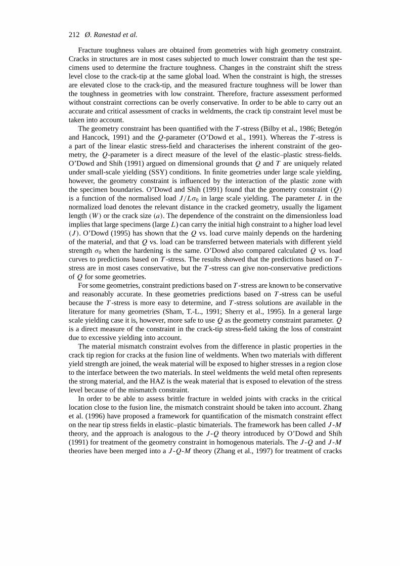
Figure 1. (a) The MBL model used for the calculations and (b) the material definitions in the model.
2.2. THE MBL MODEL
The trimaterial MBL model shown in Figure was used in the study. The model was loadedby aKI + T displacement field to simulate SSY conditions, and different levels of geometryconstraint were simulated by changing theT -stress(T ). The amplitude of the displacementfield was adjusted to giveJ = 200 N/mm after the final load step. The magnitude of theT -stress was varied in steps fromT /σ0 = −0.45 toT /σ0 = 0.5. For convenience, theT -stresswas applied before theKI -field in order to have constantT /σ0 during theKI loading.
The finite element model contains 3 materials. The mesh is very focused in the directionperpendicular to the crack(y) in order to allow for changes of the HAZ thickness, Figure 1(a).The global diameter of the MBL model(D) in Figure 1(a) is 400 mm. Figure 1(b) shows thematerial zones in the model, and Figure 2 shows the crack tip mesh and deformation. Thecrack tip has an initial opening(d) of 20µm, givingD/d = 20.000. The size of the smallestelement in the model was 4µm.
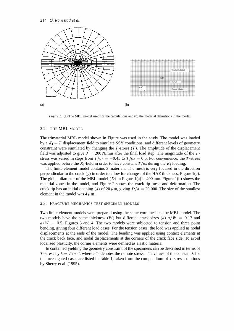
2.3. FRACTURE MECHANICSTEST SPECIMEN MODELS
Two finite element models were prepared using the same core mesh as the MBL model. Thetwo models have the same thickness(W) but different crack sizes(a) a/W = 0.17 anda/W = 0.5, Figures 3 and 4. The two models were subjected to tension and three pointbending, giving four different load cases. For the tension cases, the load was applied as nodaldisplacements at the ends of the model. The bending was applied using contact elements atthe crack back face, and nodal displacements at the corners of the crack face side. To avoidlocalised plasticity, the corner elements were defined as elastic material.
In contained yielding the geometry constraint of the specimens can be described in terms ofT -stress byk = T /σ∞, whereσ∞ denotes the remote stress. The values of the constantk forthe investigated cases are listed in Table 1, taken from the compendium ofT -stress solutionsby Sherry et al. (1995).

Quantification of geometry and material mismatch constraint215
WM
HAZ 0.6
mm
(a) (b)
Figure 2. Finite element mesh at the crack tip (a) undeformed and (b) deformed atJ = 200 N/mm, material case7-6-5, see Table 2.
26 m
m
Figure 3. Shallow cracked specimena/W = 0.17.
26 m
m
Figure 4. Deep cracked specimena/W = 0.5.
Table 1. Fracture mechanics specimen models
Case W a a/W Loading k = T/σ∞(Sham, T.-L., 1991)
SENB017 26 mm 4.4 mm 0.17 3 point bending −0.278
SENB05 26 mm 13.0 mm 0.5 3 point bending +0.318
SENT017 26 mm 4.4 mm 0.17 Tension −0.581
SENT05 26 mm 13.0 mm 0.5 Tension −0.432
216 Ø. Ranestad et al.
Table 2. Yield strength combinations in the trimaterial model
Material σWM0 σHAZ
0 σBM0 Local mismatch
combination [MPa] [MPa] [MPa] mL = σWM0 /σHAZ
0
7-6-5 700 600 500 1.167
65-6-5 650 600 500 1.083
6-6-5 600 600 500 1.0
55-6-5 550 600 500 0.927
2.4. MATERIAL PROPERTIES
The three material zones had identical elastic properties, with Young’s modulusE = 210000MPa, and Poisson ratioν = 0.3.
The material’s stress-strain relation is described by the Ramberg–Osgood power hardeninglaw (α = 1)
ε
ε0= σ
σ0+ α
(σ
σ0
)n, (1)
whereε denotes the strain,ε0 is the yield strain, defined through the yield stressσ0 and Young’smodulus asε0 = σ0/E. σ denotes the flow stress andn is the strain hardening exponent of thematerial.
The plastic properties of the base metal (BM) and the HAZ were kept constant in allcalculations, and the yield strength of weld metal was changed. The yield strength of thebase metal wasσBM
0 = 500 MPa and yield strength of the HAZσHAZ0 = 600 MPa. The
investigated weld metal (WM) yield strengths(σWM0 ) were 700, 650, 600 and 550 MPa. All
three materials had identical hardening exponentnWM = nBM = nHAZ = 14.3. The thicknessof the HAZ layer was 0.6 mm for all the calculations. The HAZ in this model representsthe coarse grained part of the HAZ in a real weldment. The effect of changes in the HAZthickness and the hardening exponents has been studied in a MBL model by the authors in(Ranestad et al., 1997, 1998). The investigated strength mismatch combinations are shownin Table 2. The material properties are regarded as typical values for modern high strengthsteels and their weldments. Thelocal mismatch, mL = σWM
0 /σHAZ0 is also shown in the table.
In addition to the mismatch combinations shown in Table 2, a calculation with homogeneousHAZ material properties (6-6-6) was carried out and used as a reference. The investigatedyield strength combinations are regarded as realistic cases for modern high strength steelweldments designed to have weld metal overmatch.
3. Material mismatch constraint in the MBL model
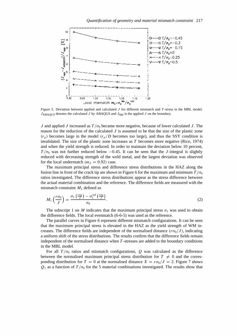
The MBL model was analysed withT /σ0 ratios ranging from−0.45 to 0.5 with all materialcombinations shown in Table 2. TheJ -integral was found to be path independent, and theagreement between applied and calculatedJ was acceptable. Figure 5 shows the deviationbetween applied and calculatedJ at appliedJ = 200 N/mm. The deviation of the calculated
Quantification of geometry and material mismatch constraint217
Figure 5. Deviation between applied and calculatedJ for different mismatch andT -stress in the MBL model.JABAQUS denotes the calculatedJ by ABAQUS andJapp is the appliedJ on the boundary.
J and appliedJ increased asT /σ0 became more negative, because of lower calculatedJ . Thereason for the reduction of the calculatedJ is assumed to be that the size of the plastic zone(rp) becomes large in the model(rp/D becomes too large), and thus the SSY condition isinvalidated. The size of the plastic zone increases asT becomes more negative (Rice, 1974)and when the yield strength is reduced. In order to maintain the deviation below 10 percent,T /σ0 was not further reduced below−0.45. It can be seen that theJ -integral is slightlyreduced with decreasing strength of the weld metal, and the largest deviation was observedfor the local undermatch(mL = 0.92) case.
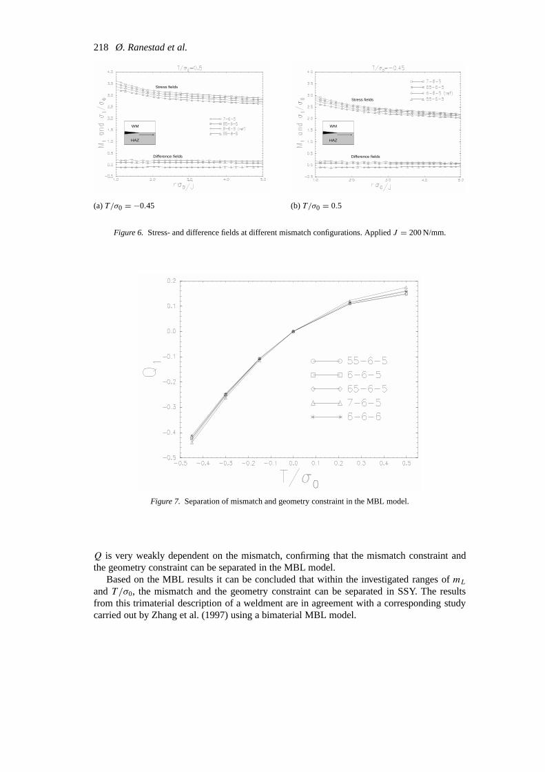
The maximum principal stress and difference stress distributions in the HAZ along thefusion line in front of the crack tip are shown in Figure 6 for the maximum and minimumT /σ0
ratios investigated. The difference stress distributions appear as the stress difference betweenthe actual material combination and the reference. The difference fields are measured with themismatch constraintM1 defined as
M1
(rσ0
J
)= σ1
(rσ0J
)− σ ref1
(rσ0J
)σ0
. (2)
The subscript 1 onM indicates that the maximum principal stressσ1 was used to obtainthe difference fields. The local evenmatch (6-6-5) was used as the reference.
The parallel curves in Figure 6 represent different mismatch configurations. It can be seenthat the maximum principal stress is elevated in the HAZ as the yield strength of WM in-creases. The difference fields are independent of the normalised distance(rσ0/J ), indicatinga uniform shift of the stress distributions. The results confirm that the difference fields remainindependent of the normalised distance whenT -stresses are added to the boundary conditionsin the MBL model.
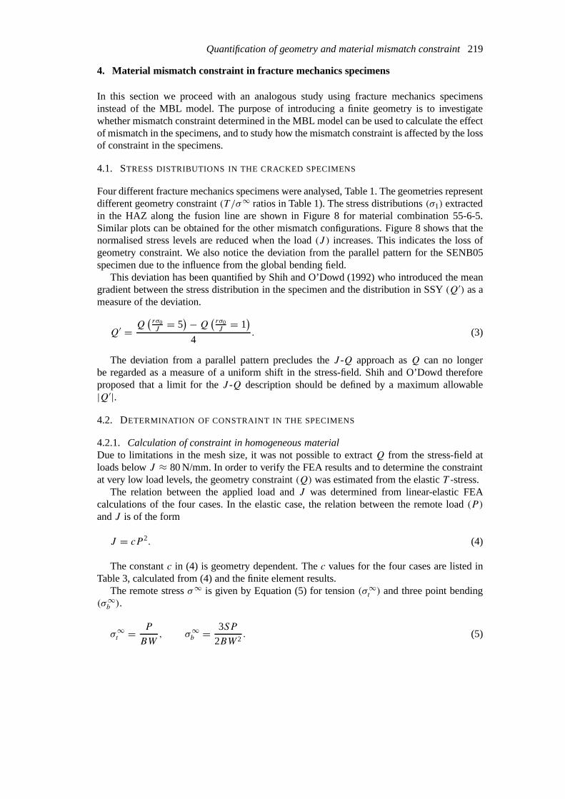
For all T /σ0 ratios and mismatch configurations,Q was calculated as the differencebetween the normalised maximum principal stress distribution forT 6= 0 and the corres-ponding distribution forT = 0 at the normalised distanceX = rσ0/J = 2. Figure 7 showsQ1 as a function ofT /σ0 for the 5 material combinations investigated. The results show that
218 Ø. Ranestad et al.
HAZ
WM
Stress fields
Difference fields
HAZ
WM
Stress fields
Difference fields
(a)T/σ0 = −0.45 (b)T/σ0 = 0.5
Figure 6. Stress- and difference fields at different mismatch configurations. AppliedJ = 200 N/mm.
Figure 7. Separation of mismatch and geometry constraint in the MBL model.
Q is very weakly dependent on the mismatch, confirming that the mismatch constraint andthe geometry constraint can be separated in the MBL model.
Based on the MBL results it can be concluded that within the investigated ranges ofmLandT /σ0, the mismatch and the geometry constraint can be separated in SSY. The resultsfrom this trimaterial description of a weldment are in agreement with a corresponding studycarried out by Zhang et al. (1997) using a bimaterial MBL model.
Quantification of geometry and material mismatch constraint219
4. Material mismatch constraint in fracture mechanics specimens
In this section we proceed with an analogous study using fracture mechanics specimensinstead of the MBL model. The purpose of introducing a finite geometry is to investigatewhether mismatch constraint determined in the MBL model can be used to calculate the effectof mismatch in the specimens, and to study how the mismatch constraint is affected by the lossof constraint in the specimens.
4.1. STRESS DISTRIBUTIONS IN THE CRACKED SPECIMENS
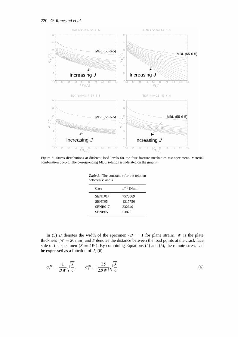
Four different fracture mechanics specimens were analysed, Table 1. The geometries representdifferent geometry constraint(T /σ∞ ratios in Table 1). The stress distributions(σ1) extractedin the HAZ along the fusion line are shown in Figure 8 for material combination 55-6-5.Similar plots can be obtained for the other mismatch configurations. Figure 8 shows that thenormalised stress levels are reduced when the load(J ) increases. This indicates the loss ofgeometry constraint. We also notice the deviation from the parallel pattern for the SENB05specimen due to the influence from the global bending field.
This deviation has been quantified by Shih and O’Dowd (1992) who introduced the meangradient between the stress distribution in the specimen and the distribution in SSY(Q′) as ameasure of the deviation.
Q′ = Q(rσ0J= 5
)−Q ( rσ0J= 1
)4
. (3)
The deviation from a parallel pattern precludes theJ -Q approach asQ can no longerbe regarded as a measure of a uniform shift in the stress-field. Shih and O’Dowd thereforeproposed that a limit for theJ -Q description should be defined by a maximum allowable|Q′|.4.2. DETERMINATION OF CONSTRAINT IN THE SPECIMENS
4.2.1. Calculation of constraint in homogeneous materialDue to limitations in the mesh size, it was not possible to extractQ from the stress-field atloads belowJ ≈ 80 N/mm. In order to verify the FEA results and to determine the constraintat very low load levels, the geometry constraint(Q) was estimated from the elasticT -stress.
The relation between the applied load andJ was determined from linear-elastic FEAcalculations of the four cases. In the elastic case, the relation between the remote load(P )
andJ is of the form
J = cP 2. (4)
The constantc in (4) is geometry dependent. Thec values for the four cases are listed inTable 3, calculated from (4) and the finite element results.
The remote stressσ∞ is given by Equation (5) for tension(σ∞t ) and three point bending(σ∞b ).
σ∞t =P
BW, σ∞b =
3SP
2BW 2. (5)
220 Ø. Ranestad et al.
Increasing J Increasing J
Increasing J Increasing J
MBL (55-6-5)MBL (55-6-5)
MBL (55-6-5) MBL (55-6-5)
Figure 8. Stress distributions at different load levels for the four fracture mechanics test specimens. Materialcombination 55-6-5. The corresponding MBL solution is indicated on the graphs.
Table 3. The constantc for the relationbetweenP andJ
Case c−1 [Nmm]
SENT017 7573369
SENT05 1317756
SENB017 332640
SENB05 53820
In (5) B denotes the width of the specimen(B = 1 for plane strain),W is the platethickness(W = 26 mm) andS denotes the distance between the load points at the crack faceside of the specimen(S = 4W). By combining Equations (4) and (5), the remote stress canbe expressed as a function ofJ , (6)
σ∞t =1
BW
√J
c, σ∞b =
3S
2BW 2
√J
c. (6)

Quantification of geometry and material mismatch constraint221
A simple estimate forQ based onT -stress can be obtained by using the piecewise linearrelations (7) suggested by Ainsworth and O’Dowd (1995) for|T /σ0| < 0.5.
Q = T
σ0, T < 0, Q = T
2σ0, T > 0. (7)
TheT -stress(T ) is proportional to the remote stress(T = kσ∞), and the factorsk havebeen calculated by Sherry et al. (1995), and are provided in Table 1 for the investigated loadcases. The equation for estimation ofQ thus becomes (8) for tension and three point bending
Tension: Three point bending:
Q = k
BWσ0
√J
c,
T
σ0< 0, Q = 3kS
2BW 2σ0
√J
c,
T
σ0< 0,
Q = k
2BWσ0
√J
c,
T
σ0> 0, Q = 3kS
4BW 2σ0
√J
c,
T
σ0> 0.
(8)
The formulation (8) is based on linear elastic conditions, and will only be a good approx-imation for low values ofJ whereJ ≈ Jel andJpl ≈ 0. In order to find the maximum loadwhere the plastic part ofJ can be neglected, the load that gives a plasticJ, Jpl = 1 N/mm werecalculated for the specimens. Kumar et al. (1981) have presented an equation for estimationof Jpl
Jpl = h(P
P0
)n+1
, (9)
whereP denotes the applied load andP0 the limit load of the specimen,h is a material andgeometry dependent constant andn is the Ramberg Osgood hardening exponent of the mater-ial. Equation (9) was solved forP with Jpl = 1 N/mm for each specimen and the maximumallowableJ values were calculated from Equation (4).
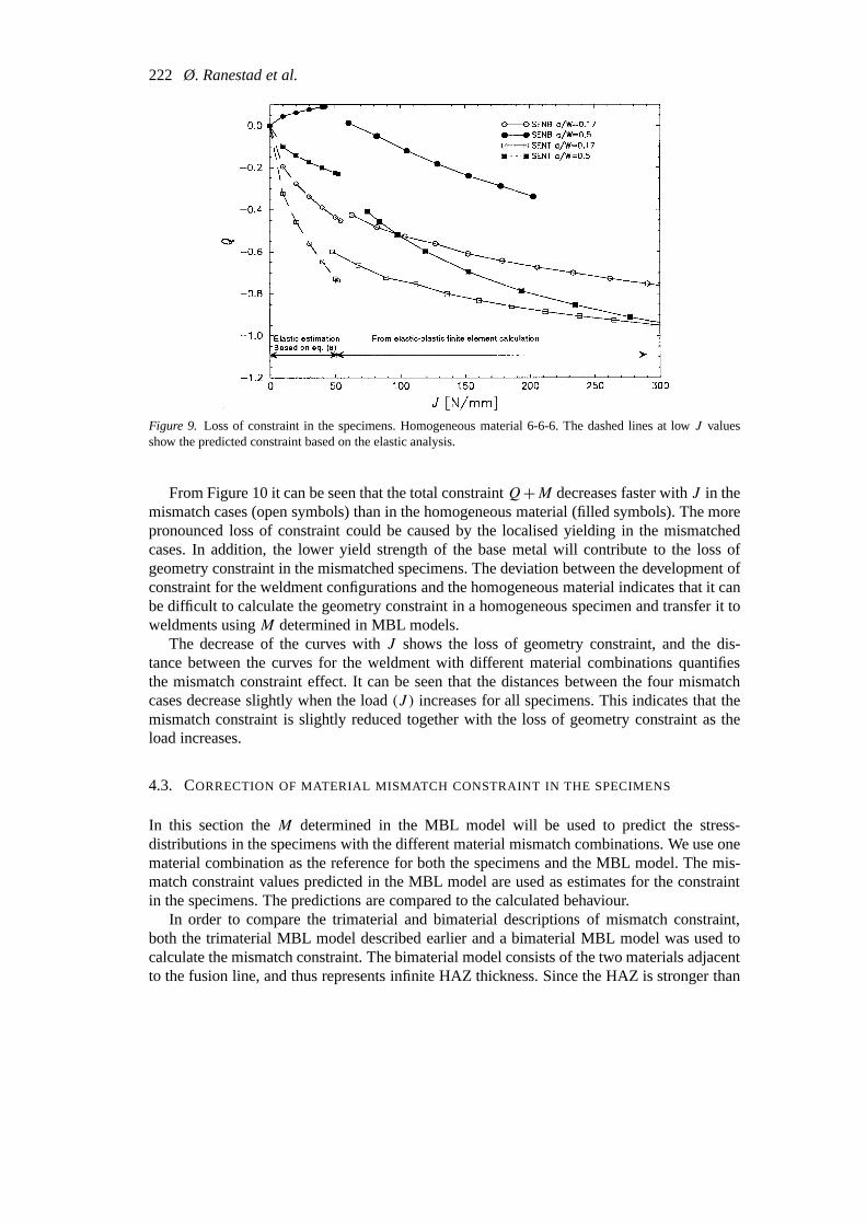
The constraintQ is plotted in Figure 9 as a function of theJ -integral. The solid linesrepresent results from the elastic plastic analysis with HAZ material properties. The dashedlines show the corresponding predictions based on (8). The elastic solution (8) is in agreementwith the finite element results. Equations (8) predict slightly lower constraint for the shortcrack cases and slightly higher constraint for the deep crack cases.
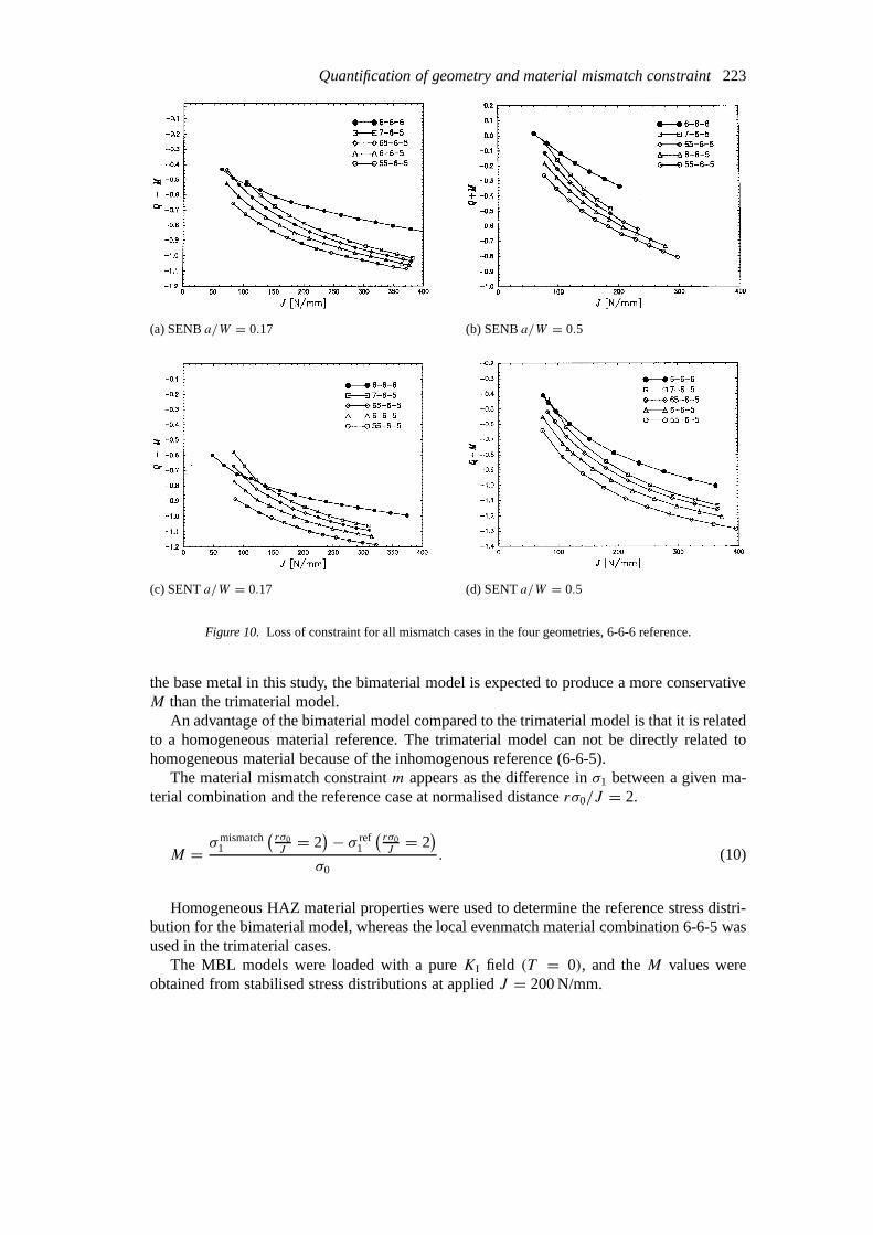
4.2.2. Calculation of constraint in the trimaterial modelIn order to compare the mismatch constraint effect in the different geometries, the total con-straint has been plotted in Figure 10 for the four load cases. The total constraint is definedas the difference between the maximum principal stress in the homogenous material’s (6-6-6) MBL solution (T = 0) and the corresponding stress distribution for the specimenswith different mismatch configurations. The differences between the stress distributions werequantified atX = rσ0/J = 2 in the HAZ, 0.02 mm from the fusion line.
In order to assure thatQ is representative for the change in constraint, limits on the max-imumQ′ were enforced. To avoid disturbances from the elements close to the crack-tip at lowload(J ),Q′ was defined as the mean deviation betweenX = 2 andX = 5 instead of betweenX = 1 andX = 5 as originally proposed by Shih and O’Dowd (1992). The limit was set toQ′ < 0.1 for all specimens.
222 Ø. Ranestad et al.
Figure 9. Loss of constraint in the specimens. Homogeneous material 6-6-6. The dashed lines at lowJ valuesshow the predicted constraint based on the elastic analysis.
From Figure 10 it can be seen that the total constraintQ+M decreases faster withJ in themismatch cases (open symbols) than in the homogeneous material (filled symbols). The morepronounced loss of constraint could be caused by the localised yielding in the mismatchedcases. In addition, the lower yield strength of the base metal will contribute to the loss ofgeometry constraint in the mismatched specimens. The deviation between the development ofconstraint for the weldment configurations and the homogeneous material indicates that it canbe difficult to calculate the geometry constraint in a homogeneous specimen and transfer it toweldments usingM determined in MBL models.
The decrease of the curves withJ shows the loss of geometry constraint, and the dis-tance between the curves for the weldment with different material combinations quantifiesthe mismatch constraint effect. It can be seen that the distances between the four mismatchcases decrease slightly when the load(J ) increases for all specimens. This indicates that themismatch constraint is slightly reduced together with the loss of geometry constraint as theload increases.
4.3. CORRECTION OF MATERIAL MISMATCH CONSTRAINT IN THESPECIMENS
In this section theM determined in the MBL model will be used to predict the stress-distributions in the specimens with the different material mismatch combinations. We use onematerial combination as the reference for both the specimens and the MBL model. The mis-match constraint values predicted in the MBL model are used as estimates for the constraintin the specimens. The predictions are compared to the calculated behaviour.
In order to compare the trimaterial and bimaterial descriptions of mismatch constraint,both the trimaterial MBL model described earlier and a bimaterial MBL model was used tocalculate the mismatch constraint. The bimaterial model consists of the two materials adjacentto the fusion line, and thus represents infinite HAZ thickness. Since the HAZ is stronger than
Quantification of geometry and material mismatch constraint223
(a) SENBa/W = 0.17 (b) SENBa/W = 0.5
(c) SENTa/W = 0.17 (d) SENTa/W = 0.5
Figure 10. Loss of constraint for all mismatch cases in the four geometries, 6-6-6 reference.
the base metal in this study, the bimaterial model is expected to produce a more conservativeM than the trimaterial model.
An advantage of the bimaterial model compared to the trimaterial model is that it is relatedto a homogeneous material reference. The trimaterial model can not be directly related tohomogeneous material because of the inhomogenous reference (6-6-5).
The material mismatch constraintm appears as the difference inσ1 between a given ma-terial combination and the reference case at normalised distancerσ0/J = 2.
M = σmismatch1
(rσ0J= 2
) − σ ref1
(rσ0J= 2
)σ0
. (10)
Homogeneous HAZ material properties were used to determine the reference stress distri-bution for the bimaterial model, whereas the local evenmatch material combination 6-6-5 wasused in the trimaterial cases.
The MBL models were loaded with a pureKI field (T = 0), and theM values wereobtained from stabilised stress distributions at appliedJ = 200 N/mm.
224 Ø. Ranestad et al.
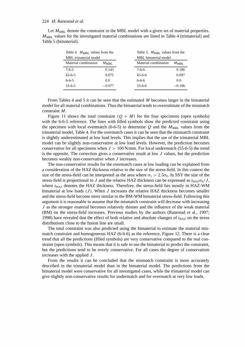
LetMMBL denote the constraint in the MBL model with a given set of material properties.MMBL values for the investigated material combinations are listed in Table 4 (trimaterial) andTable 5 (bimaterial).
Table 4.MMBL values from the
MBL trimaterial model
Material combination MMBL
7-6-5 0.143
65-6-5 0.075
6-6-5 0.0
55-6-5 −0.077
Table 5.MMBL values from the
MBL bimaterial model
Material combination MMBL
7-6-6 0.186
65-6-6 0.097
6-6-6 0.0
55-6-6 −0.106
From Tables 4 and 5 it can be seen that the estimatedM becomes larger in the bimaterialmodel for all material combinations. Thus the bimaterial tends to overestimate of the mismatchconstraintM.
Figure 11 shows the total constraint(Q + M) for the four specimens (open symbols)with the 6-6-5 reference. The lines with filled symbols show the predicted constraint usingthe specimen with local evenmatch (6-6-5) to determineQ and theMMBL values from thetrimaterial model, Table 4. For the overmatch cases it can be seen that the mismatch constraintis slightly underestimated at low load levels. This implies that the use of the trimaterial MBLmodel can be slightly non-conservative at low load levels. However, the prediction becomesconservative for all specimens whenJ > 100 N/mm. For local undermatch (55-6-5) the trendis the opposite. The correction gives a conservative result at lowJ values, but the predictionbecomes weakly non-conservative whenJ increases.
The non-conservative results for the overmatch cases at low loading can be explained froma consideration of the HAZ thickness relative to the size of the stress-field. In this context thesize of the stress-field can be interpreted as the area whereσ1 > 2.5σ0. In SSY the size of thestress-field is proportional toJ and the relative HAZ thickness can be expressed astHAZσ0/J ,wheretHAZ denotes the HAZ thickness. Therefore, the stress-field lies mostly in HAZ-WMbimaterial at low loads(J ). WhenJ increases the relative HAZ thickness becomes smallerand the stress-field become more similar to the BM-WM bimaterial stress-field. Following thisargument it is reasonable to assume that the mismatch constraint will decrease with increasingJ as the stronger material becomes relatively thinner and the influence of the weak material(BM) on the stress-field increases. Previous studies by the authors (Ranestad et al., 1997;1998) have revealed that the effect of both relative and absolute changes oftHAZ on the stressdistributions close to the fusion line are small.
The total constraint was also predicted using the bimaterial to estimate the material mis-match constraint and homogeneous HAZ (6-6-6) as the reference, Figure 12. There is a cleartrend that all the predictions (filled symbols) are very conservative compared to the real con-straint (open symbols). This means that it is safe to use the bimaterial to predict the constraint,but the predictions tend to be overly conservative. For all cases the degree of conservatismincreases with the appliedJ .
From the results it can be concluded that the mismatch constraint is more accuratelydescribed in the trimaterial model than in the bimaterial model. The predictions from thebimaterial model were conservative for all investigated cases, while the trimaterial model cangive slightly non-conservative results for undermatch and for overmatch at very low loads.
Quantification of geometry and material mismatch constraint225
(a) SENBa/W = 0.17 (b) SENBa/W = 0.5
(c) SENTa/W = 0.17 (d) SENTa/W = 0.5
Figure 11. Correction of the mismatch constraint usingM from the trimaterial MBL model.
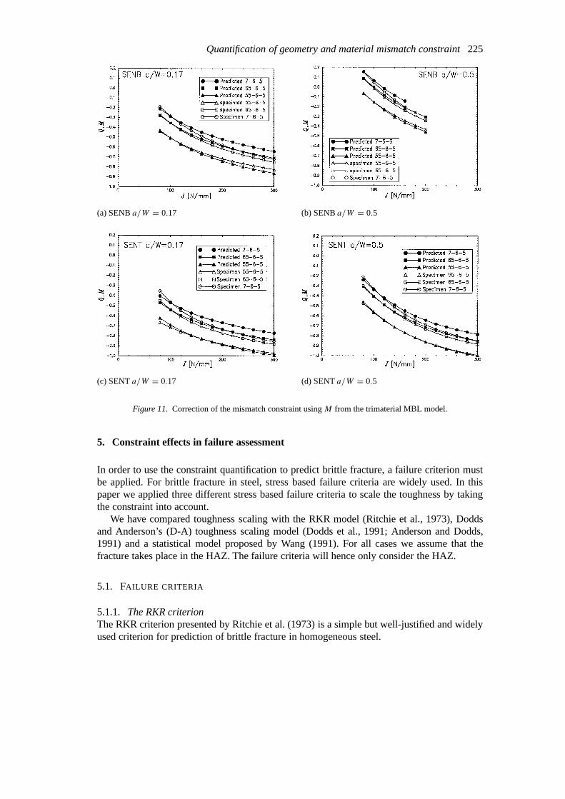
5. Constraint effects in failure assessment
In order to use the constraint quantification to predict brittle fracture, a failure criterion mustbe applied. For brittle fracture in steel, stress based failure criteria are widely used. In thispaper we applied three different stress based failure criteria to scale the toughness by takingthe constraint into account.
We have compared toughness scaling with the RKR model (Ritchie et al., 1973), Doddsand Anderson’s (D-A) toughness scaling model (Dodds et al., 1991; Anderson and Dodds,1991) and a statistical model proposed by Wang (1991). For all cases we assume that thefracture takes place in the HAZ. The failure criteria will hence only consider the HAZ.
5.1. FAILURE CRITERIA
5.1.1. The RKR criterionThe RKR criterion presented by Ritchie et al. (1973) is a simple but well-justified and widelyused criterion for prediction of brittle fracture in homogeneous steel.

226 Ø. Ranestad et al.
(a) SENBa/W = 0.17 (b) SENBa/W = 0.5
(c) SENTa/W = 0.17 (d) SENTa/W = 0.5
Figure 12. Correction of mismatch constraint withM from the bimaterial MBL model.
The RKR criterion predicts fracture when the maximum principal stress exceeds a criticalvalue (σ1/σ0)c over a microstructurally critical distancerc in front of the crack. In order toapply the RKR criterion to the MBL model, the values for(σ1/σ0)c andrc must be determined.rc should capture the fracture process zone in front of the crack-tip. Ritchie et al. originallyproposed thatrc should be approximately the size of two grains. Since we are now invest-igating an inhomogeneous material, the stresses are obtained in the HAZ close to the fusionline.
The RKR criterion can be applied in two different ways, see Figure 13(a, b). One possibilityis to fix the critical stress level (a),(σ1/σ0)c throughout the loading, while the critical distanceis increasing. Another way is to fix the critical normalised distance (b) and apply the RKRcriterion with decreasing critical stress level and increasing absolute distance.
In order to compare the two approaches the toughness was predicted as a function of thelocal mismatch as shown in Figure 13. The RKR toughness scaling was carried out accordingto (11)
Jconstraint
Jref= Xref
Xconstraint, (11)
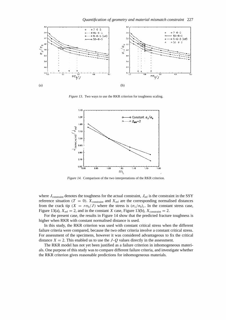
Quantification of geometry and material mismatch constraint227
(a) (b)
Figure 13. Two ways to use the RKR criterion for toughness scaling.
Figure 14. Comparison of the two interpretations of the RKR criterion.
whereJconstraintdenotes the toughness for the actual constraint,Jref is the constraint in the SSYreference situation(T = 0). XconstraintandXref are the corresponding normalised distancesfrom the crack tip(X = rσ0/J ) where the stress is(σ1/σ0)c. In the constant stress case,Figure 13(a),Xref = 2, and in the constantX case, Figure 13(b),Xconstraint= 2.
For the present case, the results in Figure 14 show that the predicted fracture toughness ishigher when RKR with constant normalised distance is used.
In this study, the RKR criterion was used with constant critical stress when the differentfailure criteria were compared, because the two other criteria involve a constant critical stress.For assessment of the specimens, however it was considered advantageous to fix the criticaldistanceX = 2. This enabled us to use theJ -Q values directly in the assessment.
The RKR model has not yet been justified as a failure criterion in inhomogeneous materi-als. One purpose of this study was to compare different failure criteria, and investigate whetherthe RKR criterion gives reasonable predictions for inhomogeneous materials.
228 Ø. Ranestad et al.
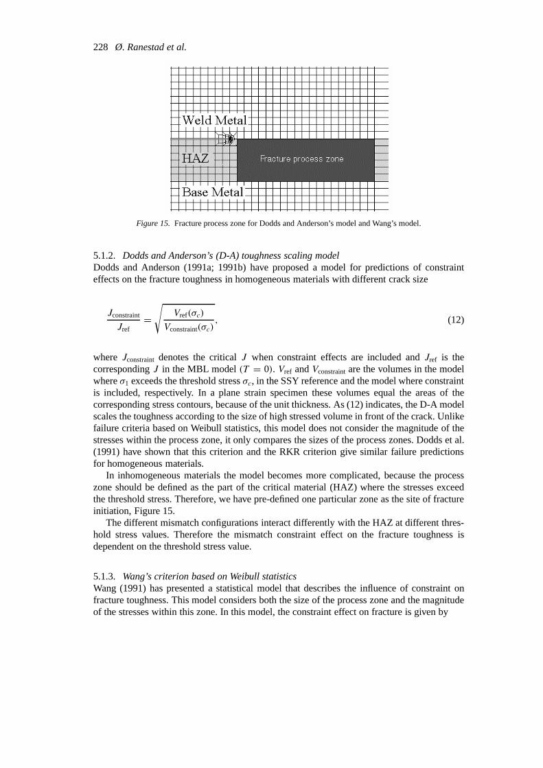
Figure 15. Fracture process zone for Dodds and Anderson’s model and Wang’s model.
5.1.2. Dodds and Anderson’s (D-A) toughness scaling modelDodds and Anderson (1991a; 1991b) have proposed a model for predictions of constrainteffects on the fracture toughness in homogeneous materials with different crack size
Jconstraint
Jref=√
Vref(σc)
Vconstraint(σc), (12)
whereJconstraint denotes the criticalJ when constraint effects are included andJref is thecorrespondingJ in the MBL model(T = 0). Vref andVconstraintare the volumes in the modelwhereσ1 exceeds the threshold stressσc, in the SSY reference and the model where constraintis included, respectively. In a plane strain specimen these volumes equal the areas of thecorresponding stress contours, because of the unit thickness. As (12) indicates, the D-A modelscales the toughness according to the size of high stressed volume in front of the crack. Unlikefailure criteria based on Weibull statistics, this model does not consider the magnitude of thestresses within the process zone, it only compares the sizes of the process zones. Dodds et al.(1991) have shown that this criterion and the RKR criterion give similar failure predictionsfor homogeneous materials.
In inhomogeneous materials the model becomes more complicated, because the processzone should be defined as the part of the critical material (HAZ) where the stresses exceedthe threshold stress. Therefore, we have pre-defined one particular zone as the site of fractureinitiation, Figure 15.
The different mismatch configurations interact differently with the HAZ at different thres-hold stress values. Therefore the mismatch constraint effect on the fracture toughness isdependent on the threshold stress value.
5.1.3. Wang’s criterion based on Weibull statisticsWang (1991) has presented a statistical model that describes the influence of constraint onfracture toughness. This model considers both the size of the process zone and the magnitudeof the stresses within this zone. In this model, the constraint effect on fracture is given by
Quantification of geometry and material mismatch constraint229
Jconstraint
Jref=
√√√√√√∫A
(σ−σuσ0
)mdA|ref∫
A
(σ−σuσ0
)mdA|constraint
, (13)
where the fracture process zonesAref andAconstraintare defined as the part of the plastic zonewhere the stressσ exceeds a threshold stress level,σu. σ denotes the opening stress(σ22) orthe maximum principal stress(σ1), and the stress values within the process zone are raised tothe powerm, andm = 2 is a typical value for this model (Wang and Parks, 1992; Karstensen,1996).
As shown in Figure 15, we have a predefined fracture process zone, the HAZ, and insteadof considering the part of the plastic zone that has stresses greater thanσu, we consider thepart of the fracture process zone in the HAZ whereσ1 > σu.
5.1.4. Comparison of the criteriaDodds et al. (1991) found that the RKR model provides a good approximation to the D-Amodel in homogeneous materials. One reason for this is the uniform shift in the whole crack-tip stress-field when the constraint(Q) changes. TheM-fields are however different fromtheQ-fields. TheQ-fields are approximately independent of the angleθ ahead of the crack,whereas theM-fields are dependent onθ (Zhang et al., 1996). The geometry constraint isuniform in the whole forward sector, whereas the mismatch constraint has its maximum valuein a smaller area close to the fusion line. This difference between mismatch and geometryconstraint suggests that ‘line-based’ failure criteria (RKR) and area/volume based criteria(Wang, D-A) can give different failure predictions for inhomogeneous materials.
The RKR criterion assumes that brittle fracture is governed by the maximum principalstress, and that the crack will advance along the crack plane when the fracture is initiated.The inhomogeneous material in this study is assumed to have a weak zone, the HAZ, wherethe fracture will take place. The RKR criterion has been applied to this situation, assumingthat the fracture should take place in the HAZ close to the fusion line. This assumption issupported by experimental results by Thaulow et al. (1994) that show that the most criticalcrack location is close to the fusion line, and that fractures often initiate from sites close to thefusion line.
We will now examine the results from Sections 3 and 4, and compare the results obtainedby different failure criteria.
5.2. TOUGHNESS SCALING IN THEMBL MODEL
In the MBL model the mismatch and geometry constraint can be separated easily as shownin Section 3. This allows the mismatch constraint to be studied separately. In the MBL modelthe stress-fields in front of the crack-tip are stabilised. Figure 16 shows the MBL stabilisedstress-distributions from HAZ, 0.02 mm from the fusion line.
The stabilised stress-distributions of the four mismatch cases were compared using thethree criteria described earlier.
5.2.1. RKR toughness scalingEquation (11) was used to scale the toughness taking the constraint into account. In order torestrictrc to the fracture process zone defined in Figure 15,Xssy 6 6 should be enforced at

230 Ø. Ranestad et al.
Figure 16. Reference stress distributions from the four mismatch cases.
Figure 17. Prediction of mismatch constraint in the MBL model with the RKR failure criterion.
J = 200 N/mm. The critical stress level must be restricted to(σ/σ0)c > 2.6 to keeprc withinthe fracture process zone.
Figure 17 shows the influence of the local mismatch on the predicted fracture toughness(Jconstraint/Jref) for different levels of the critical stress(σ1/σ0)c. For the two lowest stresslevels,rc exceeds the process zone defined in Figure 15. The detrimental effect of overmatch(mL > 1) is increasing slightly with the critical stress level. The tendency for local under-match is not clear, but the general trend is that the constraint effect on the toughness increaseswhen the critical stress level is elevated.
5.2.2. Dodds and Anderson’s toughness scaling modelFigure 18 shows the maximum principal stress areas that are used to calculate the toughnesscorrections for two different threshold stress levels. In Figure 18 the appliedJ = 200 N/mm.For this deformation level, the fracture process zone shown in Figure 18 reaches torσ0/J = 6in front of the crack tip.

Quantification of geometry and material mismatch constraint231
0 .20 0 .60 1 .00 1.40 1 .80
x [m m ]
0 .50 1 .00 1.50
x [m m ]
0 .50 1 .00 1.50
x [m m ]
0 .50 1 .00 1.50
x [m m ]
0 .50 1 .00 1.50
x [m m ]
-1 .00
-0 .50
0 .00
0 .50
1 .00
y [m
m] 7 -6 -5 65-6 -5 6-6-5 55-6 -5 6-6-6
σ /σ1 0 =2 ,6
0.20 0 .60 1 .00 1.40 1 .80
x [m m ]
0 .50 1 .00 1.50
x [m m ]
0 .50 1 .00 1.50
x [m m ]
0 .50 1 .00 1.50
x [m m ]
0 .50 1 .00 1.50
x [m m ]
-1 .00
-0 .50
0 .00
0 .50
1 .00
y [m
m] 7 -6 -5 65-6 -5 6-6-5 55-6 -5 6-6-6
σ /σ1 0 =2 ,9
Figure 18. Stress contours in the fracture process zone for two different stress levels,σ1/σ0 = 2.6 (upper) andσ1/σ0 = 2.9 (lower) for the investigated material combinations.
Figure 19. Prediction of mismatch constraint effect on fracture toughness with the D-A model. Effect of differentthreshold stress levels.
Based on the measured size of the areas in Figure 18, the toughness predictions in Figure 19were obtained using (12). The trends are similar to the RKR predictions, but stress levels lowerthanσ1/σ0 = 2.6 could not be examined, because the stress contours exceeded the fractureprocess zone.
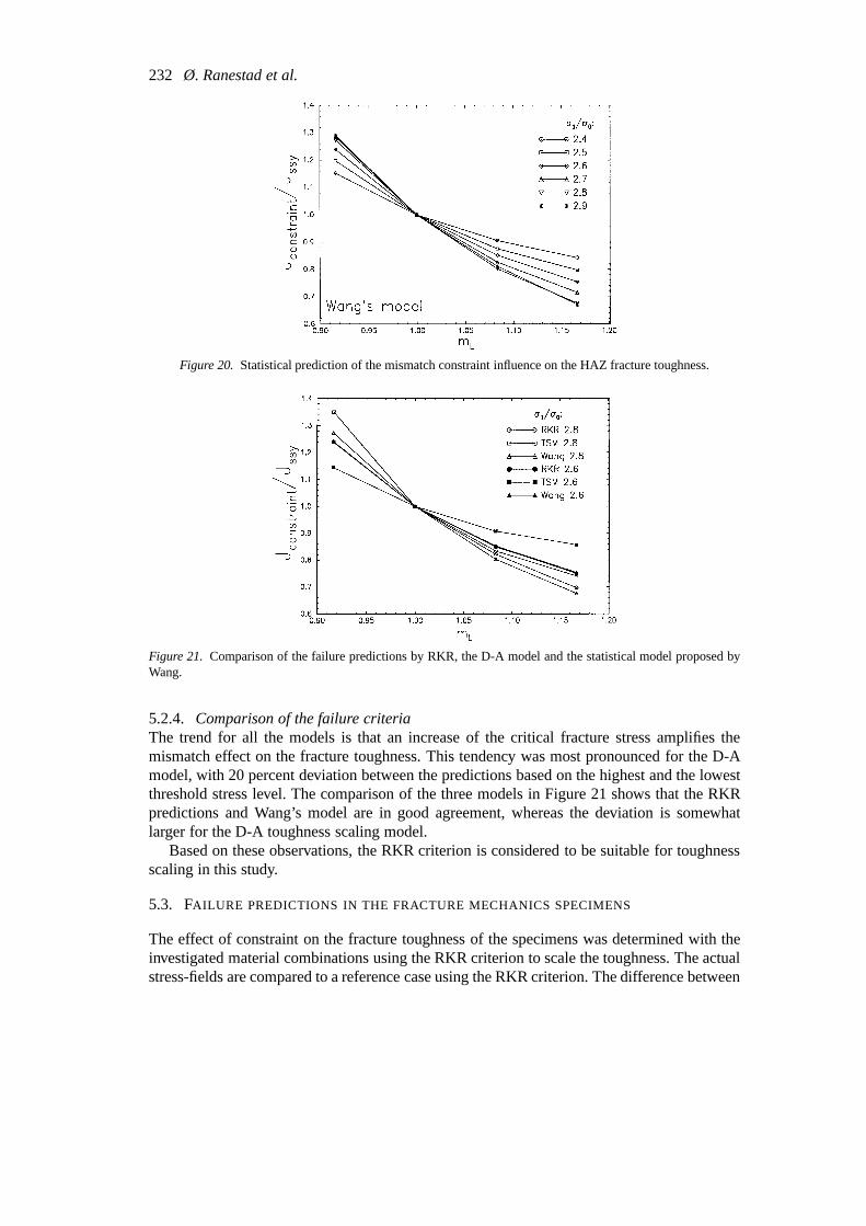
5.2.3. Toughness scaling with Wang’s modelWang’s criterion, Equation (13), was applied to the fracture process zone in the MBL model,Figure 15. The threshold stress was varied, withm = 2. The toughness predictions areshown in Figure 20. An increase of the threshold stress amplifies the mismatch effect onthe constraint. This trend is the same as predicted with the two other models.
232 Ø. Ranestad et al.
Figure 20. Statistical prediction of the mismatch constraint influence on the HAZ fracture toughness.
Figure 21. Comparison of the failure predictions by RKR, the D-A model and the statistical model proposed byWang.
5.2.4. Comparison of the failure criteriaThe trend for all the models is that an increase of the critical fracture stress amplifies themismatch effect on the fracture toughness. This tendency was most pronounced for the D-Amodel, with 20 percent deviation between the predictions based on the highest and the lowestthreshold stress level. The comparison of the three models in Figure 21 shows that the RKRpredictions and Wang’s model are in good agreement, whereas the deviation is somewhatlarger for the D-A toughness scaling model.
Based on these observations, the RKR criterion is considered to be suitable for toughnessscaling in this study.
5.3. FAILURE PREDICTIONS IN THE FRACTURE MECHANICSSPECIMENS
The effect of constraint on the fracture toughness of the specimens was determined with theinvestigated material combinations using the RKR criterion to scale the toughness. The actualstress-fields are compared to a reference case using the RKR criterion. The difference between
Quantification of geometry and material mismatch constraint233
the toughness scaling in the MBL model and in the specimens is that the stress distributionsare not stabilised. Hence, the constraint varies with the loading, and the RKR criterion wasused to calculate the effectiveJref as a function of the appliedJapp in the specimens.
The curves in the Figures 8 and 16 were curve fitted using 4th order polynomials. Thedifferent geometries were compared using the same critical distanceX = 2. This enabled usto determine the toughness scaling from the reference stress distribution and theJ -Q curve.The RKR criterion gives
Jref
Japp= Xapp
Xref. (14)
By settingXapp= 2 and curve fitting the reference stress distributionXref(σ1/σ0) and theinverse function,6ref(X) = [σ1/σ0]ref(X) as 4th order polynomials, the effectiveJ, Jref canbe expressed as
Jref = 2Japp
Xref= 2Japp
Xref(∑
ref(2)+Q). (15)
The accuracy of the RKR toughness scaling was ensured through a set of requirements forthe RKR model and the stress distributions. Limits must be defined for application of the RKRcriterion to the specimens. The set of requirements defines a ‘window’ for application of theRKR scaling approach. The requirements used for this study are presented in the next section.
5.3.1. Window for toughness predictionsIn this study a ‘window’ is proposed for applicable toughness predictions. The window definesthe limitations of the analysis.
In order to use theJ -Q-M description of the stress-fields, the stress distributions in thefinite geometry should be parallel to the reference stress distribution. The deviation wasquantified by the parameterQM ′ , which was defined as
QM ′ = QM(5)−QM(2)
3. (16)
In Equation (16)QM(X) denotes the difference field at distanceX from the crack tip. Thesubscript ‘M ’ onQ indicates that the deviation could be caused by bothQ andM. The distanceX = 2 was preferred toX = 1 to avoid influence from the crack tip at low load levels. Thelimit |QM ′ | < 0.1 was applied to ensure that the constraint parameter describes the differencefield properly. This restriction limits the maximumJapp in the SENB05 specimen.
A limit for the lowest allowableXapp > 1 was set to avoid the finite strain zone close tothe crack-tip in the model. This restriction limits the maximumQ that can be allowed in theanalysis.
In real specimens ductile crack growth will start after a certain load has been reached. Sinceductile crack growth is not included in the analyses a maximumJapp should be set, definingwhen ductile crack growth must be taken into account. The initiation of ductile tearing can bea function of the constraint as well as the deformation(J ) (Anderson et al., 1993).
The RKR criterion assumes that the fracture is controlled by the combination of a criticalstress(σ1/σ0)c and a critical distancerc. rc should be a microstructurally significant distancein the fracture process zone. The fracture process zone for brittle fracture is often defined as

234 Ø. Ranestad et al.
σσ
1
0
X=rσ /J0
MBLreference
Range for Q
Specimen
window
X=2
Q=0
Q'>0.1X<1
Figure 22. ‘Window’ for RKR toughness scaling. The shaded region indicates where the results should bediscarded.
δ/r〈2,8〉 or rσ0/J 〈1,5〉. In this study we consider the stress in the specimen at(rσ0/J ) = 2,and thereforerc always lies in the fracture process zone in the specimen. However,rc may lieoutside the fracture process zone in the reference geometry. Whenrσ0/J = 2 is fixed in thespecimen, the critical stress level can be expressed with sum of the reference stress andQ. AsQ becomes more negative during the loading, the critical stress level is reduced. By assumingthat a certain stress level(σ1/σ0)c is required to trigger cleavage fracture, a lower bound valuefor Q can be obtained. In this study we have assumed that cleavage will not occur whenQ < −1, and thus this limit is applied in the analysis. Together with the maximumJ whereductile crack growth is expected, this criterion limits the maximumJapplied in the analysis.
The proposed limits for the RKR scaling concept defines a ‘window’ for prediction ofbrittle fracture. This window is shown in Figure 22, where the shadowed areas are excludedfrom the scaling procedure. The upper limit in Figure 22 atX = 1 is defined by the maximumQ, which is a function of the hardening exponent of the reference field(n). The lower limit forthe window is set by the radial dependence limit(Q′ < 0.1) or the minimumQ for cleavage.
5.3.2. RKR toughness scaling of the specimensThe procedure outlined above was applied to the stress distributions in Figure 8. The resultsare presented in Figure 23 asJref(Japp) functions.Jref is interpreted as theeffectiveJ , or theJ that gives the same crack-tip stress distribution in the MBL reference model asJapp gives inthe examined geometry.
Figure 23 shows the failure predictions for the four investigated specimens. The opensymbols show the curves from the mismatched specimens. The predictions based on the MBLcorrections for the material mismatch constraint are shown with filled symbols in Figure 23.The predictions are based on the constraint curves shown in Figure 11, with the local even-match 6-6-5 used as the reference. It is apparent that the SENB05 specimen has a much highereffectiveJ than the other specimens. The predictions based on the MBL calculation of themismatch constraint are conservative for the overmatch cases in all specimens. However, theeffectiveJ is weakly underestimated for the local undermatch cases in bending with the MBL
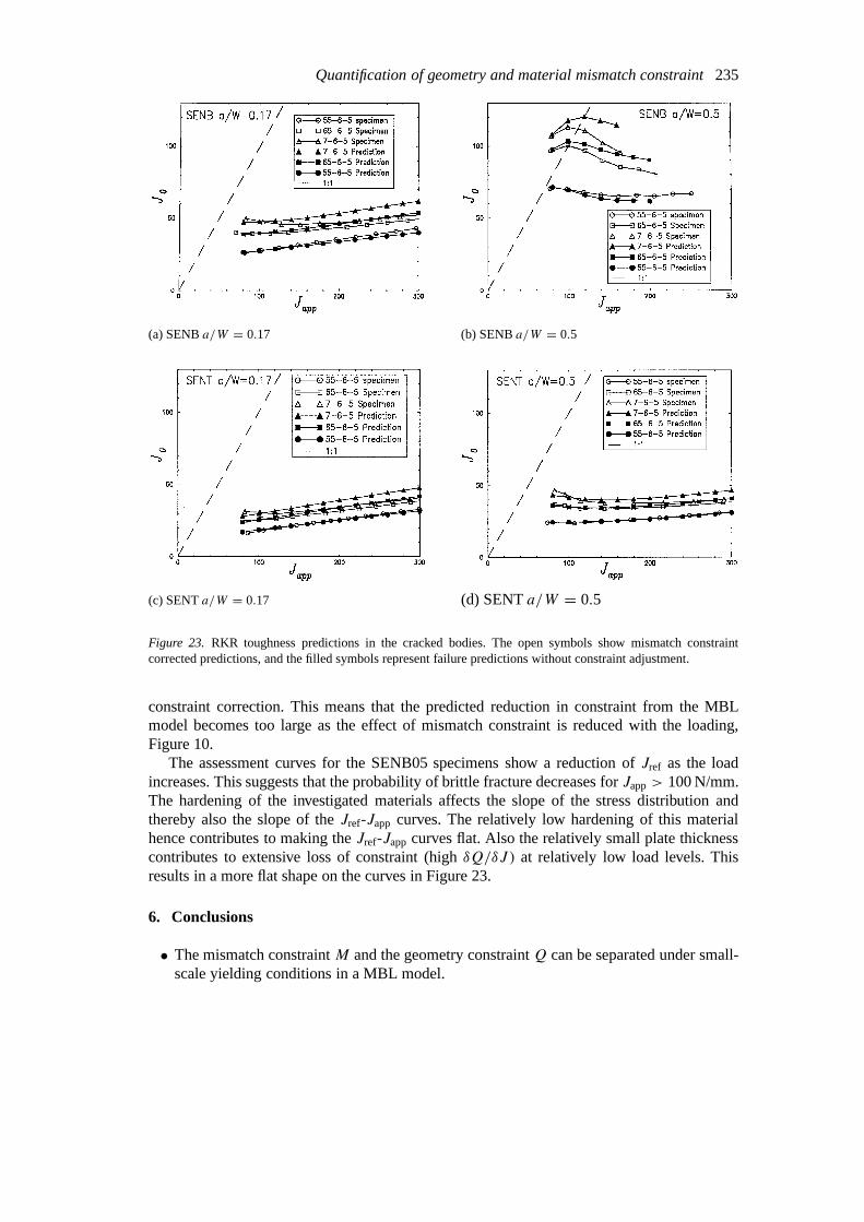
Quantification of geometry and material mismatch constraint235
(a) SENBa/W = 0.17 (b) SENBa/W = 0.5
(c) SENTa/W = 0.17 (d) SENTa/W = 0.5
Figure 23. RKR toughness predictions in the cracked bodies. The open symbols show mismatch constraintcorrected predictions, and the filled symbols represent failure predictions without constraint adjustment.
constraint correction. This means that the predicted reduction in constraint from the MBLmodel becomes too large as the effect of mismatch constraint is reduced with the loading,Figure 10.
The assessment curves for the SENB05 specimens show a reduction ofJref as the loadincreases. This suggests that the probability of brittle fracture decreases forJapp> 100 N/mm.The hardening of the investigated materials affects the slope of the stress distribution andthereby also the slope of theJref-Japp curves. The relatively low hardening of this materialhence contributes to making theJref-Japp curves flat. Also the relatively small plate thicknesscontributes to extensive loss of constraint (highδQ/δJ ) at relatively low load levels. Thisresults in a more flat shape on the curves in Figure 23.
6. Conclusions
• The mismatch constraintM and the geometry constraintQ can be separated under small-scale yielding conditions in a MBL model.
236 Ø. Ranestad et al.
• For the investigated fracture mechanics specimens and material combinations in this study,it was found that the loss of constraint is different in the weldments than in homogeneousHAZ material. Therefore, the behaviour of the weldments could not be predicted from ahomogeneous specimen and a trimaterial MBL model.• The mismatch constraint is slightly reduced together with the loss of geometry constraint
when large scale yielding develops.• The change in mismatch constraint from an inhomogeneous reference situation was pre-
dicted from mismatch constraint valuesM obtained from a MBL model. The predic-tions were conservative for overmatched specimens, and slightly non-conservative forundermatched specimens.• Predictions obtained with the trimaterial model and an inhomogeneous reference material
combination were more accurate than predictions from a WM/HAZ bimaterial with ahomogeneous reference material. The bimaterial predictions were on the conservativeside.• Three different stress-based failure criteria for predictions of the mismatch effect on the
cleavage toughness in the MBL model were compared. The predictions were similar, andin all cases the predictions depend on the selected critical stress level. The RKR criterionwas preferred due to its simplicity compared to the other criteria.• A window for valid cleavage predictions with theJ -Q-M framework and the RKR failure
criterion was proposed.• By correcting a reference specimen with mismatch constraint values obtained in the MBL
model, the effectiveJ was predicted from the RKR failure criterion.
Acknowledgements
This work has been supported by Kværner ASA, through a PhD grant for Øyvind Ranestad,within the research project ‘Ship for the future’.
The work has also received support from The Research Council of Norway (Programmefor Supercomputing) through a grant of computing time.
References
Ainsworth, R.A. and O’Dowd, N.P. (1995). Constraint in the failure assessment diagram approach for fractureassessment.Journal of Pressure Vessel Technology117, 260–267.
Anderson, T.L. and Dodds, R.H., Jr. (1991). Specimen size requirements for fracture toughness testing in thetransition region.Journal of Testing and Evaluation19, 123–134.
Anderson, T.L., Vanaparthy, N.M.R. and Dodds, R.H., Jr. (1993). Predictions of specimen size dependence onfracture toughness for cleavage and ductile tearing.Constraint Effects in Fracture, ASTM STP 1171(Editedby E.M. Hackett, K.-H. Schwalbe and R.H. Dodds), American Society for Testing and Materials, Philadelphia,pp. 473–491.
Betegón, C., and Hancock, J.W. (1991). Two-parameter characterization of elastic–plastic crack-tip fields.Journalof Applied Mechanics58, 104–110.
Bilby, B.A., Cardew, G.E., Goldthorpe, M.R. and Howard, I.C. (1986). A finite element investigation of the effectof specimen size and geometry on the fields of stress and strain at the tip of stationary cracks, inSize Effectsin Fracture, I Mech. E., London, pp. 37–46.
Dodds, R.H. Jr., Anderson, T.L. and Kirk, M.T. (1991a). A framework to correlatea/W ratio effects on elastic–plastic fracture toughness(Jc). International Journal of Fracture48, 1–22.
Dodds, R.H., Jr., Shih, C.F. and Anderson, T.L. (1991b).International Journal of Fracture64, 101–133.Karstensen, A.D. (1996).Constraint Estimation Schemes in Fracture Mechanics, PhD. thesis, Univ of Glasgow,
UK.
Quantification of geometry and material mismatch constraint237
Kumar, V., German, M.D. and Shih, C.F. (1981).An Engineering Approach for Elastic–Plastic Fracture AnalysisEPRI report NP 1931, Electric Power Research Institute, Palo Alto, CA, USA.
O’Dowd, N.P. (1995). Applications of two parameter approaches in elastic–plastic fracture mechanics.Engineer-ing Fracture Mechanics52/3, 445–465.
O’Dowd, N.P. and Shih, C.F. (1991). Family of crack-tip fields characterized by a triaxiality parameter – I: Fractureapplications.Journal of the Mechanics and Physics of Solids40, 939–963.
O’Dowd, N.P. and Shih, C.F. (1991). Family of crack-tip fields characterized by a triaxiality parameter – I:Structure of the fields.Journal of the Mechanics and Physics of Solids39, 989–1015.
Ranestad, Ø., Zhang, Z.L. and Thaulow, C. (1997). Quantification of mismatch constraint in an elastic–plastictrimaterial system.Mis-matching of Interfaces and Welds(Edited by K.-H. Schwalbe and M. Kocak), GKSSResearch Center Publications, Geestacht, FRG, pp. 749–758.
Ranestad, Ø., Zhang, Z.-L. and Thaulow, C. (1998). Two-parameter (J-M) description of crack-tip stress-fields foran idealized weldment in small scale yielding.International Journal of Fracture88/4, 315–333.
Rice, J.R. (1974). Limitations to the small scale yielding approximation for crack tip plasticity.Journal of theMechanics and Physics of Solids22, 17–26.
Ritchie, R.O., Knott, J.F. and Rice, J.R. (1973). On the relationship between critical tensile stress and fracturetoughness in mild steel.Journal of the Mechanics and Physics of Solids21, 395–410.
Sham, T.-L. (1991). The determination of the elasticT -term using higher order weight functions.InternationalJournal of Fracture48, 81–102.
Sherry, A.H., France, C.C. and Goldthorpe, M.R. (1995).Fatigue and Fracture of Engineering Materials andStructures18(1), 141–155.
Shih, C.F. and O’Dowd, N.P. (1992). A fracture mechanics approach based on a toughness locus, inProceedingsof TWI/EWI/IS International Conference on Shallow Crack Fracture Mechanics, TWI, Cambridge, UK.
Thaulow, C., Hauge, M., Paauw, A.J., Toyoda, M. and Minami, F. (1994). Effect of notch TIP location in CTODtesting of the heat affected zone of steel weldments, inProceedings from ECF 10: Structural Integrity:Experiments, Models and Applications(Edited by Schwalbe, K.-H. and Berger, C.), Berlin, pp. 1053–1066.
Thaulow, C. and Toyoda, M. (1997). Strength mis-match effect on fracture behaviour of HAZ.Mis-matchingof Interfaces and Welds(Edited by K.-H. Schwalbe and M. Kocak), GKSS Research Center Publications,Geestacht, FRG, pp. 75–98.
Thaulow, C., Hauge, M., Zhang, Z.L., Ranestad, Ø. and Fattroini, F. (1988). On the interrelationship betweenfracture toughness and material mismatch for cracks located at the fusion line of weldments, to appear inspecial issue ofEngineering Fracture Mechanicson strength mis-match effect.
Wang, Y.-Y. (1991).A Two-parameter Characterisation of Elastic–Plastic Crack-tip Fields and Applications toCleavage Fracture. Ph.D. thesis, Dept. of Mechanical Engineering, Massachusetts Institute of Technology.
Wang, Y.Y. and Parks, D.M. (1992). Characterisation of constraint effect on cleavage toughness usingT -stress, inProceedings of TWI/EWI/IS International Conference on Shallow Crack Fracture Mechanics, TWI,Cambridge, UK.
Zhang, Z.L., Hauge, M. and Thaulow, C. (1996). Two-parameter characterization of the near-tip stress fields for abi-material elastic–plastic interface crack.International Journal of Fracture79, 65–83.
Zhang, Z.L., Hauge, M. and Thaulow, C. (1997). The effect ofT -stress on the near tip stress field of an interfacecrack.Proceedings of the 9th International Conference on Fracture, Sydney, (Edited by B.L. Karihalo, Y.-W.Mai, M.I. Ripley and R.O. Ritchie), 2643–2650.
Zhang, Z.L., Thaulow, C. and Hauge, M. (1997). Effects of crack size and weld metal mismatch on the HAZcleavage toughness of wide plates.Engineering Fracture Mechanics57/6, 653–664.