quality pricing and release time optimal market …

RESEARCH ARTICLE

QUALITY, PRICING, AND RELEASE TIME:OPTIMAL MARKET ENTRY STRATEGY FOR

SOFTWARE-AS-A-SERVICE VENDORS

Haiyang FengCollege of Management and Economics, Tianjin University,

Tianjin 300072, CHINA {[email protected]}

Zhengrui JiangCollege of Business, Iowa State University,

Ames, Iowa 50011-2027 U.S.A. {[email protected]}

Dengpan LiuSchool of Economics and Management, Tsinghua University,

Beijing, CHINA 100084 {[email protected]}

Appendix

Proofs

1 Proof of Equilibrium Solutions (8) and (9)

(7)

( )( )

0

0

ˆmax

ˆmax 1

ˆ. . 1

0, 0

DL

DH

D DL L

p

D DH H

p

D

D DL H

p

p

s tp p

π θ θ

π θ

θ θ

= −

= −

≤ ≤

≥ ≥

Substituting into (7), and solving the first order conditions yields( ) ( )θ θ γ γ

τ τ γ γD p p

q qHD

LD

L H

H B L B H L= − − −

− − −0

(8.1)

( ) ( ) ( )( ) ( )( )

( ) ( ) ( )( ) ( )( )

0 0

0 0

2 1 23

1 2 1 23

H B L B L H

H B L B L H

q qDH

q qDL

p

p

θ τ τ θ γ γ

θ τ τ θ γ γ

− − − − +∗

− − − − +∗

=

=

MIS Quarterly Vol. 42 No. 1—Appendix/March 2018 A1

Feng, Jiang, & Liu/Optimal Market Entry Strategy for New SaaS Vendors

A2 MIS Quarterly Vol. 42 No. 1‒Appendix/March 2018

and ∗ = ( ) ( ) ( ) ( ) ( )( ) ( )∗ = ( ) ( ) ( ) ( )( )( ) ( ) ∗ = ( ) ( ) ( ) ( )( )( ) ( ) (8.2)

Thus, the two vendors’ profits are ∗ = ( ) ( ) ( ) ( )( )( ) ( )∗ = ( ) ( ) ( ) ( )( )( ) ( ) (8.3)

The prices and demands of the two vendors in this equilibrium are positive if and only if ( ) − ( ) ≥ ( + 2 ).

When ( ) − ( ) < ( + 2 ), the price of Vendor L in Equilibrium (8) is negative, hence we have a new equilibrium

solution by setting ∗ = 0: ∗ = ( ) − ( ) + (1 − )∗ = 0 (9.1)

∗ = ∗ = 1 −∗ = 0 (9.2)

∗ = ( ) − ( ) (1 − ) + (1 − )∗ = 0 (9.3)

□□

2 Proof of Lemma 1

After product B’ release, the quality difference of the two products remains unchanged because the two vendors have the same post-release quality improvement rate. Therefore, from equations (8) and (9), the equilibrium prices and profit rates for the two products remain constant in the duopoly stage. In addition, equilibrium prices and profit rates for the two products increase with quality difference of the two products

upon the release of product B because ∗ ≥ 0 and

∗ ≥ 0 hold ( = ( ) − ( )). □□

3 Proof of Observation 1

From equilibrium (9.1) through (9.3), in the zero-profit region, i.e., ( ) − ( ) < ( + 2 ), the price and profit rate of

Vendor L are both zero. Since is positive, any increase in or would expand this zero-profit region of Vendor L. □□


MIS Quarterly Vol. 42 No. 1‒Appendix/March 2018 A3

4 Proof of Proposition 1

maxΠ = [ ( ) − ( )]( − ) − , ≤[ ( ) − ( )]( − ) − , > (10)

The necessary conditions for to be the globally optimal solution of (10) are < < (A1)

Π ( ) > Π (0) (A2)

Condition (A1) ensures that belongs to the feasible region ( , ), and (A2) is needed because is the more profitable solution than 0.

Since = and = + − , condition (A1) is equivalent to

∆ < −

The profit difference between the two local optimal solutions is Π ( ) − Π (0) = − − − ∆ + + −

It can be shown that Π ( ) > Π (0) leads to Δ < Δ or Δ > Δ

where Δ = + + − + + + and Δ = + + + + + + .

Note that Δ > − ; thus, Δ > Δ violates condition (A1). Therefore, conditions (A1) and (A2) hold only when Δ satisfies

Δ ≤ Δ

where Δ = min + + − + + + , − .

Therefore, if Δ ≤ Δ , is the optimal release time; otherwise, Vendor B should release its product at time 0. Correspondingly, the profits of the two vendors are Π∗ = ∆ , >

4 − 2 − 2 + 4 + 4 − 2 , ∆ ≤

Π∗ = ∆ , ∆ >Π ∗ + Π ∗, ∆ ≤

where Π ∗ = ∗ + − and Π ∗ = − − . □□



5 Proof of Corollary 1 When ∗ = 0, the prices of product A and B take the forms ∗ = Δ∗ = Δ

The condition ∈ 0, leads to > ; thus, the equilibrium price of product B is lower than that of product A.

When Vendor B releases its product at ∗ = + − , the prices of product A and B become

∗ = ( + ∗ − )∗ = ( + ∗ − )

Since > , we conclude that the price of product B is higher than that of product A when the new entrant adopts the late-release

strategy. □□

6 Proof of Corollary 2

As stated in Proposition 1, when ≤ , Vendor B’s profit is given by Π∗ = 4 − 2 − 2 + 4 + 4 − 2

which is a quadric function of . As increases, Π∗ reaches its minimum at = + . Since < + , Π∗ decreases with

when ≤ . When > , the profit of Vendor B is given by Π∗ = ∆

which is an increasing function of ∆ . Therefore, Vendor B’s profit increases monotonically with when > . □□


(1) When ∆ > Δ , the two vendors’ profits are given by

Π∗ = ∆Π∗ = ∆

Thus, ∗ = Δ > 0,

∗ = > 0, ∗ = Δ > 0, and

∗ = > 0.

(2) When ∆ ≤ Δ , the vendors’ profits are

Π∗ = Π ∗ + Π ∗Π∗ = − − + + −



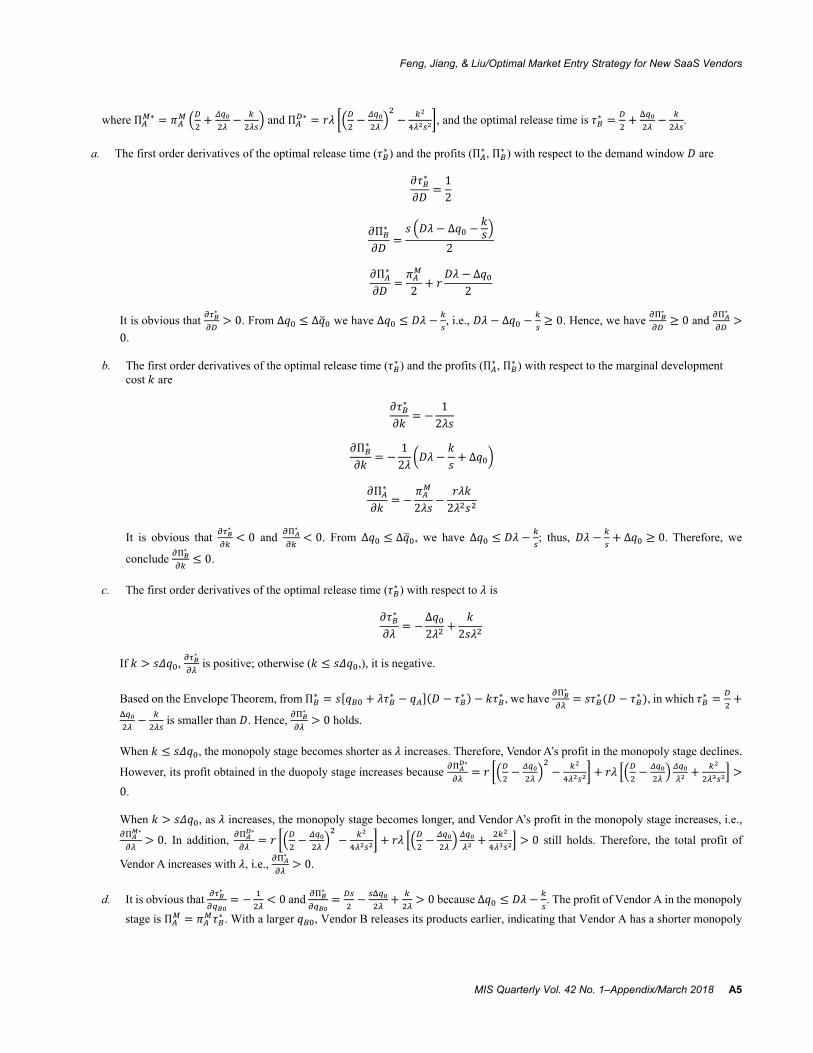
where Π ∗ = + − and Π ∗ = − − , and the optimal release time is ∗ = + − .

a. The first order derivatives of the optimal release time ( ∗ ) and the profits (Π∗ , Π∗ ) with respect to the demand window are

∗ = 12

Π∗ = − Δ −2

Π∗ = 2 + − Δ2

It is obvious that ∗ > 0. From ∆ ≤ Δ we have ∆ ≤ − , i.e., − ∆ − ≥ 0. Hence, we have

∗ ≥ 0 and ∗ >0.

b. The first order derivatives of the optimal release time ( ∗ ) and the profits (Π∗ , Π∗ ) with respect to the marginal development

cost are ∗ = − 12

Π∗ = − 12 − + Δ

Π∗ = −2 − 2

It is obvious that ∗ < 0 and

∗ < 0. From ∆ ≤ Δ , we have ∆ ≤ − ; thus, − + Δ ≥ 0. Therefore, we

conclude ∗ ≤ 0.

c. The first order derivatives of the optimal release time ( ∗ ) with respect to is

∗ = −Δ2 + 2

If > , ∗ is positive; otherwise ( ≤ ,), it is negative.

Based on the Envelope Theorem, from Π∗ = [ + ∗ − ]( − ∗ ) − ∗ , we have ∗ = ∗ ( − ∗ ), in which ∗ = +− is smaller than . Hence,

∗ > 0 holds.

When ≤ , the monopoly stage becomes shorter as increases. Therefore, Vendor A’s profit in the monopoly stage declines.

However, its profit obtained in the duopoly stage increases because ∗ = − − + − + >0.

When > , as increases, the monopoly stage becomes longer, and Vendor A’s profit in the monopoly stage increases, i.e., ∗ > 0. In addition,

∗ = − − + − + > 0 still holds. Therefore, the total profit of

Vendor A increases with , i.e., ∗ > 0.

d. It is obvious that ∗ = − < 0 and

∗ = − + > 0 because ∆ ≤ − . The profit of Vendor A in the monopoly

stage is Π = ∗ . With a larger , Vendor B releases its products earlier, indicating that Vendor A has a shorter monopoly



stage; thus, its profit in the monopoly stage decreases, i.e. ∗ < 0. Furthermore, the first order derivatives of Π ∗ with respect

to is ∗ = − . Because ∆ < − , we have

∗ > 0. □□

8 Proof of Lemma 2 From the equilibrium outcomes (8) and (9), if ∈ , , Vendor B’s profit rate is zero; thus it is not profitable for Vendor B to release its product in this zero-profit region. If Vendor B releases its product in its winner-take-all region ( , ), the demand of Vendor A drops to

zero, i.e., product A is driven out of market. Because = 0, > 0, and < 0, both regions expand as increase. Similarly, the two

regions expand as increases ( = 0, > 0, and < 0). □□

9 Equilibrium Prices and Demands Corresponding to Different Release Strategies

a. When Vendor B adopts the instant-release strategy, ∗ = ( ) ( )( )

∗ = ( ) ( )( ) (A3)

∗ = ( ) ( )( )∗ = ( ) ( )( ) (A4)

b. When Vendor B adopts the late-release strategy and ∗ ∈ , , ∗ = 0∗ = ( ∗ − Δ ) + (1 − ) (A5)

∗ = 0∗ = 1 − (A6)

c. When Vendor B adopts the late-release strategy and ∗ ∈ [ , ],

∗ = ( )( ∗ ) ( )( )∗ = ( )( ∗ ) ( )( ) (A7)



∗ = ( )( ∗ ) ( )( )∗∗ = ( )( ∗ ) ( )( )∗ (A8)

□□

10 Proof of Proposition 2

From equilibrium solutions (8) and (9), if Vendor B adopts the instant-release strategy, its optimal price, demand, and profit are given by ∗ = ( ) ( )( )∗ = ( ) ( )( )Π∗ = [( ) ( )( )]

Then, we have ∗ > 0, because

∗ > 0 and ∗ > 0.

When Vendor B releases its products at ( > ), a. If ∈ , , the profit of Vendor B is given by

Π = [ ( − Δ )(1 − ) + (1 − ) ]( − ) − which decreases with .

b. If ∈ [ , ], the profit of Vendor B is given by Π = 19 [(2 − )( − Δ ) − (1 − )(2 + )] − Δ − − ( − ) −

Then, we have ΠΔ = ( − )[(2 − )( − Δ ) − (1 − )(2 + )]9 2 + (3 − ) − (2 − )( − Δ )( − Δ − − )

≥ yields 2 + (3 − ) − (2 − )( − Δ ) ≤ 0. Thus, we have ≤ 0, implying that Vendor B’s profit decreases with Δ .

Therefore, when Vendor B releases its products after , its profit curve will move downwards as the initial quality gap Δ becomes larger. Hence, Vendor B’s maximal profit obtained by releasing products in [ , ] decreases with Δ . Vendor B’s profit obtained from the instant-release strategy increases with , while that obtained from the late-release strategy decreases with it. Therefore, there exists a threshold value for the initial quality gap, under which the late-release strategy is more profitable than the instant-release strategy. Vendor B’s profit maximization problem is, therefore,



maxΠ = [( )( ) ( )( )] ( − ) − , < [ ( + − )(1 − ) + (1 − ) ]( − ) − , < <[( )( ) ( )( )] ( − ) − , ≤ ≤ (12)

s.t. ∈ 0, ∪ ( , ]

When ∈ [ , ], it is intractable to obtain the locally optimal release time in this interval. When = 0, the only root of = 0 in [ , ] takes the form, = 4 + 3(Δ + + )4 + ( − Δ − − )[ − Δ − − + ]4

where = ( ) (2 + ) − 8 − 8 .

Hence, when = 0, in time interval [ , ], and are the only two possible optimal solutions for Vendor B. Furthermore, we have < 0; based on the envelop theorem, the locally optimal release time of Vendor B in [ , ] decreases with , i.e.,

∗ < 0.

Therefore, we conclude that when adopting the late-release strategy, Vendor B should not release its product later than time or time , whichever occurs later. That is, ∗ < max , . □□


From Proposition 2, Vendor B cannot release its products later than time or time , whichever occurs later. Thus, if a Type I late-release strategy is adopted, must be larger than and the optimal release time must fall within [ , ). In addition, Lemma 2 indicates that, when product B is released after , products A and B coexist in the market and serve the low-end and the high-end markets, respectively. Regarding Type II late release strategy, Lemma 2 proves that when product B is released in the winner-take-all time interval ( , ), product A will be driven out of the market. □□

12 Proof of Lemma 3

As shown in Table 2, when Vendor B adopts the instant-release strategy, its product quality is lower than Vendor A’s. Thus, Vendor B’s profit rate decreases with or . Hence, Vendor B’s total profit also decreases with the level of incompatibility. When Vendor B adopts the late-release strategy, and the optimal release time falls within ( , ), we have Π ( ) = [ ( + − )(1 − ) + (1 − ) ]( − ) −

Obviously, Vendor B’s profit curve moves upward as becomes larger and its maximal profit increases with . When Vendor B adopts the late-release strategy, and the optimal release time falls within [ , ], Vendor B’s profit is Π ( ) = [( )( ) ( )( )] ( − ) −

Thus, for a given , we have ( ) < 0 and

( ) > 0. Therefore, when releasing its product in [ , ], Vendor B’s maximal profit

increases with , while decreases with . □□



13 Equilibrium with Switching Cost Considered

Case I In this case, the vendors’ objectives are to maximize their respective profit rates:

max = −max = 1 − (A9)

s.t. ≤ ≤ ≤ ≤ 1

Based on the fulfilled expectation equilibrium, solving (A9) yields the following equilibrium solution: ∗ = ( ) ( ) ( ) ( )( )

∗ = ( ) ( ) ( ) ( )( ) (A10.1)

∗ = ( ) ( ) ( ) ( ) ( )( ) ( )∗ = ( ) ( ) ( ) ( )( )( ) ( ) ∗ = ( ) ( ) ( ) ( )( )( ) ( )

(A10.2)

Π ∗ = ( ) ( ) ( ) ( )( )( ) ( )Π ∗ = ( ) ( ) ( ) ( )( )( ) ( ) (A10.3)

This equilibrium holds when ≤ ≤ ∗ ≤ ∗ < 1. Case II In this case, the profit-maximization problem is max = − + −max = 1 − + − (A11)

s.t. ≤ ≤ < ≤ 1

The corresponding equilibrium prices and profit rates are ∗ = ( ) ( )( )

∗ = ( ) ( )( ) (A12.1)

∗ = ( ) ( )( )( )∗ = ( ) ( )( )( )

(A12.2)



Π ∗ = ( ) ( )( )( )Π ∗ = ( ) ( )( )( ) (A12.3)

This equilibrium holds when ∗ ≥ 0, ∗ ≥ 0, ∗ ≥ 0, and ∗ ≥ 0. Case III The two vendors’ objectives are to maximize their respective profit rates: max = 1 −max = − (A13)

s.t. ≤ < ≤ 1

The equilibrium prices and profit rates take the following forms: ∗ = ( )( ) ( )( )

∗ = ( )( ) ( )( ) (A14.1)

∗ = ( )( ) ( ) ( )∗ = ( )( ) ( )( ) ∗ = ( )( ) ( )( )

(A14.2)

Π ∗ = ( )( ) ( )( )Π ∗ = ( )( ) ( )( ) (A14.3)

The above equilibrium holds when ≤ < ∗ ≤ 1. □□ 14 Model Extension II: A Model with Quadratic Cost Function In this subsection, we analyze the case in which marginal development cost is a quadratic function of development time: = (A15)

We find that under this new quadratic cost function, the equilibrium prices, demands, and profit rates shown in (8) and (9) remain valid. In the full-compatibility scenario, the optimal release time for Vendor B can be derived by maxΠ = (Δ − )( − ) − , ≤( − Δ )( − ) − , > (A16)

where = . By solving (A16), we have two local optima: = 0 and = , corresponding to instant-release and late-release

strategies, respectively. Proposition 1still holds under a quadratic cost function, but the threshold value takes a different form:



Δ = min + [ ( + ) + − ( + )ℎ],

where ℎ = ( ) ( ).

If the initial quality gap is larger than Δ , Vendor B should release its products immediately; otherwise, the late-release strategy is preferred. In the partial-compatibility scenario, Vendor B’s profit maximization problem is,

maxΠ = [( )( ) ( )( )] ( − ) − , < [ ( + − )(1 − ) + (1 − ) ]( − ) − , < <[( )( ) ( )( )] ( − ) − , ≤ ≤ (A17)

s.t. ∈ 0, ∪ ( , ] As shown in Figure A1, the result in the partial-compatibility scenario still holds when the quadratic cost function is adopted.

(a) Optimal Market Entry Strategy

(b) Maximal Profit

( = 20, = 0.1, = 2, = 0, = 0.5, = 0.1, = 1.25, and , ∈ [0,0.5]) Figure A1. Optimal Market Entry Strategy and Maximal Profit of Vendor B

In summary, our main analytically findings still hold even when a quadratic cost function is adopted. □□ 15 Model Extension III: A Model with Unequal Quality Improvement Rates In this subsection, we investigate the scenario where the two vendors have unequal post-release quality improvement rates. After , the quality levels of product A and B are given by ( ) = + , ∈ [0, ]( ) = + + ( − ), ∈ [ , ] (A18)

where and are post-release quality improvement rates of product A and B, respectively. Let denote the difference between and , i.e., = − . > 0 ( < 0) indicates that, after product B’s release, product A’s quality increases faster (slower) than that of product B.



From the solutions of optimal profit rates, i.e., Equations (8.3) and (9.3), we have the following findings. In the case of unequal post-release quality improvement rates, as the quality gap between the two products in the duopoly stage increases (decreases) over time, the profit rates of both vendors increase (decrease) over time. The explanation for this finding is as follow. A larger quality gap leads to less competition between the two vendors, so both the prices and profit rates for the two products increase. So long as the post-release quality improvement doesn’t change the sign of ( ) − ( ) , another finding follows immediately: If product B has a lower post-release quality improvement rate ( > ), the profit rate of Vendor B associated with the instant-release strategy increases over time, whereas its profit rate associated with the late-release strategy decreases over time. On the other hand, if the post-release quality improvement rate of product B is higher ( < ), the profit rate of Vendor B associated with the instant-release strategy decreases over time, whereas its profit rate associated with the late-release strategy increases over time. In Table A1 below, we summarize the changes in quality gap and profit rates of the two vendors when their post-release quality improvement rates are different.

Table A1. Changes in Profit Rates of the Two Vendors

Strategy Quality Gap (Over time)

Profit rate of Vendor B (Over time)

Profit rate of Vendor A (Over time) > 0 Instant-Release Increase Increase Increase Late-Release Decrease Decrease Decrease < 0 Instant-Release Decrease Decrease Decrease Late-Release Increase Increase Increase

As shown in Table A1, if Vendor B has a lower post-release quality improvement rate than Vendor A, the instant-release strategy is preferred by the new entrant; otherwise, the unequal quality improvement rates improve Vendor B’s profit in the late-release strategy. This result is similar in spirit to Proposition 1. In both cases, the new vendor should adopt the instant-release strategy if it is difficult to compete with the incumbent on product quality, and choose the late-release strategy otherwise. A closer examination of Table A1 reveals that the release strategy preferred by the new entrant is always the one that results in an increasing quality gap over time. This is because a larger quality gap can effectively reduce the competition between the two products.

(a) Optimal Market Entry Strategy

( = 20, = 0.1, = 2, = 1.5, ∈ [0,0.05], ∈ [0,0.05], = 0, = 0.2, = = 0.1, = 0.1)

Figure A2. Optimal Market Entry Strategy and Maximal Profit of Vendor B

0 0.005 0.01 0.015 0.02 0.025 0.03 0.035 0.04 0.045 0.050

0.005

0.01

0.015

0.02

0.025

0.03

0.035

0.04

0.045

0.05

λ2B

λ 2A

Instant Release

Late Release

0

0.01

0.02

0.03

0.04

0.05

00.01

0.020.03

0.040.05

0

0.5

1

1.5

2

λ2Bλ2A

Prof

it of

Ven

dor

B

Instant Release Late Release

(b) Maximal Profit



Figure A2(a) shows that an increase in may change Vendor B’s optimal strategy from late-release to instant-release, while an increase in has the opposite effect. As shown in Figure A2(b), in the region where the instant-release strategy is optimal, Vendor B attains its highest

profit when = 0.05 and = 0. Similarly, when the values of ( , ) falls within the region where the late-release strategy is optimal, Vendor B attains its highest profit at ( , ) = (0, 0.05). □□

16 Model Extension IV: A Model with Partial Market Coverage

In the full-compatibility scenario, to ensure that the market is fully covered, the value of , representing the type of customers with the minimum marginal willingness-to-pay, should satisfy − ∗ + (1 − ) > 0 (A19)

in which L represents the product with lower quality and ∗ = ( )( ). From (A19), we have

> ( ) ( )( ) (A20)

Similarly, in the partial-compatibility scenario, when ( − ) ≥ ( + 2 ), should satisfy

− ∗ + ∗ + ∗ > 0 (A21)

Because and ∗ are non-negative terms, ∗ > ∗ is a sufficient condition for (A21). Substituting ∗ =( )( ) ( )( ) and ∗ = ( )( ) ( )( )

into ∗ > ∗, we have

> − − − (A22)

When ( − ) < ( + 2 ), i.e., in the zero-profit region for Vendor L, the full-coverage assumption holds unconditionally

because the price of L drops to zero. Therefore, we conclude that when the intensity of network effects is sufficiently high, our assumption that “the value of is set in such a way that all consumers will purchase either A or B in the duopoly stage” can be satisfied.

Figure A3. Market Segmentation

Figure A3 shows the market segmentation under partial market coverage. denotes the type of consumer who is indifferent between purchasing product L and making no purchasing. In this case, the two vendors’ equilibrium prices when the two products are fully compatible are

∗ = ( − )∗ = ( − ) (A23)

Both ∗ and ∗ equal zero when = ; thus, Lemma 2 still holds under partial market coverage. That is, the new entrant should not release its product at the time when its product quality equals that of the incumbent.

For robustness check, we analyze an extreme case in which the intensity of network effects equals zero ( = 0). In this case, the optimal prices, demand, and profit rates for the two vendors are

1

H L No purchase



∗ = ( )∗ = ( ) ∗ =∗ = ∗ = ( )( )∗ = ( )( ) (A24)

The optimal release time can be obtained by solving maxΠ = ( ) ( )[ ( ) ( )][ ( ) ( )] ( − ) − , ≤( )[ ( ) ( )][ ( ) ( )] ( − ) − , > (A25)

Since the optimal release time for the new entrant is analytically intractable, we choose to graphically compare the profits of Vendor B under full and partial market coverage. The solid and the dotted lines in Figure A4 represent the profit curves of Vendor B under full coverage, and partial coverage, respectively. As shown in the figure, although the optimal release time and profit for Vendor B under partial coverage differs from those under full coverage, the pattern of two-local-optima remains unchanged.

(a) = 0.25

(b) = 0.5

(c) = 0.75

( = 20, = 0.1, = 2, = 0, = 0.2 (for full coverage only), = 0.1)

Figure A4. Profit Comparison We have also examined whether instant release and late release remain the only feasible release strategies under partial market coverage. We find that, theoretically speaking, a third possible strategy does exist. Specifically, under partial market coverage, after adopting the instant-release strategy, Vendor B’s product quality is lower than Vendor A’s. In this case, if Vendor B increases its product quality, more low-end consumers will be attracted to purchase product B, i.e., becomes smaller. However, when we assume to be sufficiently large to ensure that the market is fully covered, such expansion in low-end market wouldn’t exist. Therefore, using to assure full-market coverage could in some cases eliminate Vendor B’s incentive to increase its product quality. As discussed above, when we relax the full-market coverage assumption by considering the partial-coverage scenario (i.e., ∈ [0,1]), a higher quality for product B will attract more low-end customers; thus, it is theoretically possible that the “releasing on time 0” strategy could change to “releasing in (0, ),” which allows Vender B to further increase its quality even when it determines to target the low end market. However, further analysis reveals that even in the partial-coverage scenario (i.e., ∈ [0,1]), Vendor B prefers “releasing at time 0” to “releasing in (0, )” in most cases. This is because although delaying the release from time 0 to a later time in (0, ) might lead to a slightly larger market share for Vendor B, the benefit of releasing its product at time 0 can still be higher for the following reasons:

(a) Releasing at time 0 would give Vendor B the longest possible duration of service. (b) Releasing at time 0 would save Vendor B’s development cost. (c) Releasing at time 0 would help Vendor B better differentiate its product from the incumbent’s in quality, thus reducing competition

between the vendors.

To examine the tradeoffs, we have conducted additional numerical experiments. We find that “releasing at time 0” can still be a viable strategy under various circumstances, whereas “releasing in (0, )” can be optimal only when the initial quality of vendor B’s product is close to 0. Recall that the scenario we consider in this study is that Vendor B’s product is ready for release at time 0, which indicates that product B’s initial quality cannot be too low. Therefore, although it is theoretically possible for “releasing in (0, )” to be an optimal strategy, the probability that it would occur under the scenario we consider is very small.

0 2 4 6 8 10 12 14 16 18 20-2

-1.5

-1

-0.5

0

0.5

1

1.5

2

2.5

3

τB

Prof

it of

Ven

dor

B

Full CoveragePartial Coverage

0 2 4 6 8 10 12 14 16 18 20-2

-1.5

-1

-0.5

0

0.5

1

1.5

2

2.5

τB

Prof

it of

Ven

dor

B


0 2 4 6 8 10 12 14 16 18 20-2

-1.5

-1

-0.5

0

0.5

1

1.5

2

τB

Prof

it of

Ven

dor

B


quality pricing and release time optimal market …

Documents