quality in phrase mining - massachusetts institute of...
TRANSCRIPT
Universitat des SaarlandesMax-Planck-Institut fur Informatik
Quality in Phrase Mining
Masterarbeit im Fach Informatik
Masters Thesis in Computer Science
von / by
Alekh Jindal
angefertigt unter der Leitung von / supervised by
Prof. Dr. Jens Dittrich
betreut von / advised by
Prof. Dr. Gerhard Weikum
begutachtet von / reviewers
Prof. Dr. Jens Dittrich
Prof. Dr. Gerhard Weikum
Saarbrucken, December 28, 2009

i
Non-plagiarism Statement
Hereby I confirm that this thesis is my own work and that I have documented all sources
used.
(Alekh Jindal)
Saarbrucken, December 28, 2009
Declaration of Consent
Herewith I agree that my thesis will be made available through the library of the Com-
puter Science Department.
(Alekh Jindal)
Saarbrucken, December 28, 2009
ii

iii

Abstract
Phrase snippets of large text corpora like news articles or web search results offer great
insight and analytical value. While much of the prior work is focussed on efficient storage
and retrieval of all candidate phrases, little emphasis has been laid on the quality of
the result set. In this thesis, we define phrases of interest and propose a framework
for mining and post-processing interesting phrases. We focus on the quality of phrases
and develop techniques to mine minimal-length maximal-informative sequences of words.
The techniques developed are streamed into a post-processing pipeline and include exact
and approximate match-based merging, incomplete phrase detection with filtering, and
heuristics-based phrase classification. The strategies aim to prune the candidate set of
phrases down to the ones being meaningful and having rich content. We characterize
the phrases with heuristics- and NLP-based features. We use a supervised learning
based regression model to predict their interestingness. Further, we develop and analyze
ranking and grouping models for presenting the phrases to the user. Finally, we discuss
relevance and performance evaluation of our techniques. Our framework is evaluated
using a recently released real world corpus of New York Times news articles.

v

Acknowledgements
I would like to express my sincere gratitude to Prof. Jens Dittrich and Prof. Gerhard
Weikum for giving me an opportunity to work under their supervision. Regular discus-
sions with Prof. Jens Dittrich were helpful in keeping up the momentum and motivating
to further meander through the course of the work. I came to admire and aspire his
disruptive approach to research. Periodic reviews and soul searching with Prof. Gerhard
Weikum were greatly helpful in getting the big picture and deciding upon the further
course of action. It was a privilege to know and learn from his depth of experiences.
I am also thankful to Klaus Berberich for providing the initial support for the existing
system, Tobias Leidinger and Sven Obser for their wonderful coordination in phrases
analytics server and web interfaces development and to Jorg Schad for providing the
reliable hardware and cluster support.
Finally, I am grateful to my parents, relatives and friends for fusing in me the desire to
learn and the will to achieve.
vi

vii

Contents
Abstract iv
Acknowledgements vi
List of Figures xii
List of Tables xiv
List of Algorithms xvi
1 Introduction 11.1 Motivation . . . . . . . . . . . . . . . . . . . . . . . . . . . . . . . . . . . 11.2 Need for Phrase Mining . . . . . . . . . . . . . . . . . . . . . . . . . . . . 21.3 Need for Quality in Phrase Mining . . . . . . . . . . . . . . . . . . . . . . 21.4 Contributions . . . . . . . . . . . . . . . . . . . . . . . . . . . . . . . . . . 31.5 Outline of the Thesis . . . . . . . . . . . . . . . . . . . . . . . . . . . . . . 3
2 Related Work 52.1 Term level analysis . . . . . . . . . . . . . . . . . . . . . . . . . . . . . . . 52.2 Term level multi-dimensional view . . . . . . . . . . . . . . . . . . . . . . 62.3 Phrase level analysis . . . . . . . . . . . . . . . . . . . . . . . . . . . . . . 6
2.3.1 KeyPhrases . . . . . . . . . . . . . . . . . . . . . . . . . . . . . . . 62.3.2 Auto-completion Systems . . . . . . . . . . . . . . . . . . . . . . . 72.3.3 Multidimensional Content eXploration (MCX) . . . . . . . . . . . 72.3.4 Phrase Forward Index . . . . . . . . . . . . . . . . . . . . . . . . . 9
3 Domain Model and Interestingness 113.1 Domain Model . . . . . . . . . . . . . . . . . . . . . . . . . . . . . . . . . 113.2 Interesting Phrases . . . . . . . . . . . . . . . . . . . . . . . . . . . . . . . 12
4 System Architecture 154.1 System Overview . . . . . . . . . . . . . . . . . . . . . . . . . . . . . . . . 154.2 Post Processing . . . . . . . . . . . . . . . . . . . . . . . . . . . . . . . . . 16
4.2.1 Merging . . . . . . . . . . . . . . . . . . . . . . . . . . . . . . . . . 174.2.2 Filtering . . . . . . . . . . . . . . . . . . . . . . . . . . . . . . . . . 184.2.3 Classification . . . . . . . . . . . . . . . . . . . . . . . . . . . . . . 19
viii
Contents ix
4.2.4 Ranking . . . . . . . . . . . . . . . . . . . . . . . . . . . . . . . . . 194.2.5 Grouping . . . . . . . . . . . . . . . . . . . . . . . . . . . . . . . . 20
4.3 User Interface . . . . . . . . . . . . . . . . . . . . . . . . . . . . . . . . . . 214.4 Conclusion . . . . . . . . . . . . . . . . . . . . . . . . . . . . . . . . . . . 22
5 Merge Strategies 235.1 Exact Merge . . . . . . . . . . . . . . . . . . . . . . . . . . . . . . . . . . 23
5.1.1 Prefix Merge . . . . . . . . . . . . . . . . . . . . . . . . . . . . . . 245.1.2 Suffix Merge . . . . . . . . . . . . . . . . . . . . . . . . . . . . . . 265.1.3 Prefix-Suffix Merge . . . . . . . . . . . . . . . . . . . . . . . . . . . 27
5.2 Approximate Merge . . . . . . . . . . . . . . . . . . . . . . . . . . . . . . 305.2.1 Stop-Word Merge . . . . . . . . . . . . . . . . . . . . . . . . . . . . 325.2.2 Synonym Merge . . . . . . . . . . . . . . . . . . . . . . . . . . . . 335.2.3 Other Merges . . . . . . . . . . . . . . . . . . . . . . . . . . . . . . 35
5.3 Conclusion . . . . . . . . . . . . . . . . . . . . . . . . . . . . . . . . . . . 35
6 Filter Strategies 376.1 Static Rule based filtering . . . . . . . . . . . . . . . . . . . . . . . . . . . 37
6.1.1 Custom filter . . . . . . . . . . . . . . . . . . . . . . . . . . . . . . 376.1.2 Prefix/Suffix filter . . . . . . . . . . . . . . . . . . . . . . . . . . . 396.1.3 Parts-of-Speech (POS) filter . . . . . . . . . . . . . . . . . . . . . . 40
6.2 Corpus-based filtering . . . . . . . . . . . . . . . . . . . . . . . . . . . . . 426.2.1 FussyTree filter . . . . . . . . . . . . . . . . . . . . . . . . . . . . . 42
6.3 Conclusion . . . . . . . . . . . . . . . . . . . . . . . . . . . . . . . . . . . 46
7 Phrase Classification 477.1 Feature Extraction . . . . . . . . . . . . . . . . . . . . . . . . . . . . . . . 477.2 Feature Selection . . . . . . . . . . . . . . . . . . . . . . . . . . . . . . . . 527.3 Training Classifier . . . . . . . . . . . . . . . . . . . . . . . . . . . . . . . 537.4 Label Prediction (Classification) . . . . . . . . . . . . . . . . . . . . . . . 547.5 Classifier based filtering . . . . . . . . . . . . . . . . . . . . . . . . . . . . 55
7.5.1 Threshold filter . . . . . . . . . . . . . . . . . . . . . . . . . . . . . 557.6 Conclusion . . . . . . . . . . . . . . . . . . . . . . . . . . . . . . . . . . . 56
8 Phrase Ranking 578.1 Ranking Within and Across Labels . . . . . . . . . . . . . . . . . . . . . . 578.2 Ranking Parameters . . . . . . . . . . . . . . . . . . . . . . . . . . . . . . 58
8.2.1 Local and Global Frequency . . . . . . . . . . . . . . . . . . . . . . 588.2.2 Classification Distribution . . . . . . . . . . . . . . . . . . . . . . . 598.2.3 Document Relevance . . . . . . . . . . . . . . . . . . . . . . . . . . 598.2.4 Size of document collection . . . . . . . . . . . . . . . . . . . . . . 598.2.5 Document Rank . . . . . . . . . . . . . . . . . . . . . . . . . . . . 598.2.6 Global Statistics . . . . . . . . . . . . . . . . . . . . . . . . . . . . 60
8.3 Ranking Functions . . . . . . . . . . . . . . . . . . . . . . . . . . . . . . . 608.4 Conclusion . . . . . . . . . . . . . . . . . . . . . . . . . . . . . . . . . . . 61
9 Phrase Grouping 639.1 Group by Clustering . . . . . . . . . . . . . . . . . . . . . . . . . . . . . . 63

Contents x
9.2 Similarity based Grouping . . . . . . . . . . . . . . . . . . . . . . . . . . . 649.2.1 Noun Similarity . . . . . . . . . . . . . . . . . . . . . . . . . . . . . 669.2.2 Cosine Similarity . . . . . . . . . . . . . . . . . . . . . . . . . . . . 67
9.3 Conclusion . . . . . . . . . . . . . . . . . . . . . . . . . . . . . . . . . . . 67
10 Experimental Evaluation and Results 6910.1 Experimental Setup . . . . . . . . . . . . . . . . . . . . . . . . . . . . . . 69
10.1.1 System Configuration . . . . . . . . . . . . . . . . . . . . . . . . . 6910.1.2 Data set . . . . . . . . . . . . . . . . . . . . . . . . . . . . . . . . . 7010.1.3 Experiments . . . . . . . . . . . . . . . . . . . . . . . . . . . . . . 70
10.2 Results . . . . . . . . . . . . . . . . . . . . . . . . . . . . . . . . . . . . . . 7110.2.1 Ranked Results . . . . . . . . . . . . . . . . . . . . . . . . . . . . . 7110.2.2 Grouped Results . . . . . . . . . . . . . . . . . . . . . . . . . . . . 72
10.3 Evaluation . . . . . . . . . . . . . . . . . . . . . . . . . . . . . . . . . . . . 7210.3.1 Precision . . . . . . . . . . . . . . . . . . . . . . . . . . . . . . . . 7210.3.2 Recall . . . . . . . . . . . . . . . . . . . . . . . . . . . . . . . . . . 7410.3.3 Precision/Recall Variation in Post-Processing . . . . . . . . . . . . 7510.3.4 Filtering Effectiveness . . . . . . . . . . . . . . . . . . . . . . . . . 7510.3.5 Processing Latencies . . . . . . . . . . . . . . . . . . . . . . . . . . 7710.3.6 Cross Validation . . . . . . . . . . . . . . . . . . . . . . . . . . . . 7810.3.7 Normalized Discounted Cumulative Gain (NDCG) . . . . . . . . . 79
10.4 Discussion . . . . . . . . . . . . . . . . . . . . . . . . . . . . . . . . . . . . 8010.5 Conclusion . . . . . . . . . . . . . . . . . . . . . . . . . . . . . . . . . . . 81
11 Further Optimizations 8311.1 Forward Index Translation . . . . . . . . . . . . . . . . . . . . . . . . . . . 8311.2 Forward Index Pruning . . . . . . . . . . . . . . . . . . . . . . . . . . . . 85
11.2.1 Pushing Merge down to Indexing . . . . . . . . . . . . . . . . . . . 8611.2.2 Pushing Filter down to Indexing . . . . . . . . . . . . . . . . . . . 86
11.3 Conclusion . . . . . . . . . . . . . . . . . . . . . . . . . . . . . . . . . . . 87
12 Conclusion and Future Work 8912.1 Future Work . . . . . . . . . . . . . . . . . . . . . . . . . . . . . . . . . . 91
A Ranked Phrases 93
B Grouped Phrases 99
Bibliography 105

xi

List of Figures
4.1 System Overview . . . . . . . . . . . . . . . . . . . . . . . . . . . . . . . . 164.2 Processing Pipeline . . . . . . . . . . . . . . . . . . . . . . . . . . . . . . . 174.3 Merge Post-Processing Stage . . . . . . . . . . . . . . . . . . . . . . . . . 174.4 Filter Post-Processing Stage . . . . . . . . . . . . . . . . . . . . . . . . . . 184.5 Classify Post-Processing Stage . . . . . . . . . . . . . . . . . . . . . . . . 194.6 Rank Post-Processing Stage . . . . . . . . . . . . . . . . . . . . . . . . . . 204.7 Group Post-Processing Stage . . . . . . . . . . . . . . . . . . . . . . . . . 204.8 Phrase Mining Interface . . . . . . . . . . . . . . . . . . . . . . . . . . . . 22
5.1 Merge Strategies . . . . . . . . . . . . . . . . . . . . . . . . . . . . . . . . 24
6.1 Filter Strategies . . . . . . . . . . . . . . . . . . . . . . . . . . . . . . . . . 38
7.1 Classification Steps . . . . . . . . . . . . . . . . . . . . . . . . . . . . . . . 487.2 Phrase Classification . . . . . . . . . . . . . . . . . . . . . . . . . . . . . . 55
8.1 Phrase Ranking . . . . . . . . . . . . . . . . . . . . . . . . . . . . . . . . . 58
10.1 Precision by Query . . . . . . . . . . . . . . . . . . . . . . . . . . . . . . . 7310.2 Recall by Query . . . . . . . . . . . . . . . . . . . . . . . . . . . . . . . . 7410.3 Precision Variation . . . . . . . . . . . . . . . . . . . . . . . . . . . . . . . 7510.4 Recall Variation . . . . . . . . . . . . . . . . . . . . . . . . . . . . . . . . . 7610.5 Filtering Effectiveness . . . . . . . . . . . . . . . . . . . . . . . . . . . . . 7610.6 Filtering Scalability . . . . . . . . . . . . . . . . . . . . . . . . . . . . . . 7710.7 Processing Latency . . . . . . . . . . . . . . . . . . . . . . . . . . . . . . . 7810.8 Cross Validation . . . . . . . . . . . . . . . . . . . . . . . . . . . . . . . . 7910.9 NDCG . . . . . . . . . . . . . . . . . . . . . . . . . . . . . . . . . . . . . . 80
11.1 Forward Index Translation . . . . . . . . . . . . . . . . . . . . . . . . . . . 8411.2 Phrase Layout . . . . . . . . . . . . . . . . . . . . . . . . . . . . . . . . . 8511.3 POS Tag Encoding . . . . . . . . . . . . . . . . . . . . . . . . . . . . . . . 8511.4 Named Entity Tag Encoding . . . . . . . . . . . . . . . . . . . . . . . . . 86
xii

xiii

List of Tables
2.1 Phrase Inverted Index . . . . . . . . . . . . . . . . . . . . . . . . . . . . . 82.2 Phrase Forward Index . . . . . . . . . . . . . . . . . . . . . . . . . . . . . 9
5.1 Prefix Merge . . . . . . . . . . . . . . . . . . . . . . . . . . . . . . . . . . 245.2 Suffix Merge . . . . . . . . . . . . . . . . . . . . . . . . . . . . . . . . . . . 265.3 Prefix-Suffix Merge . . . . . . . . . . . . . . . . . . . . . . . . . . . . . . . 285.4 Levenshtein Distance . . . . . . . . . . . . . . . . . . . . . . . . . . . . . . 315.5 Stop-word merge . . . . . . . . . . . . . . . . . . . . . . . . . . . . . . . . 335.6 Synonym merge . . . . . . . . . . . . . . . . . . . . . . . . . . . . . . . . . 34
6.1 Custom Filter Rules . . . . . . . . . . . . . . . . . . . . . . . . . . . . . . 386.2 Prefix/Suffix Filter Rules . . . . . . . . . . . . . . . . . . . . . . . . . . . 396.3 POS Filter Rules . . . . . . . . . . . . . . . . . . . . . . . . . . . . . . . . 416.4 POS Filter Rules . . . . . . . . . . . . . . . . . . . . . . . . . . . . . . . . 41
7.1 Phrase Labels . . . . . . . . . . . . . . . . . . . . . . . . . . . . . . . . . . 53
10.1 Training and Testing Queries . . . . . . . . . . . . . . . . . . . . . . . . . 7110.2 Top-10 Phrases . . . . . . . . . . . . . . . . . . . . . . . . . . . . . . . . . 7110.3 Grouped Phrases . . . . . . . . . . . . . . . . . . . . . . . . . . . . . . . . 72
xiv

xv
List of Algorithms
5.1 Prefix Merge . . . . . . . . . . . . . . . . . . . . . . . . . . . . . . . . . . . 25
5.2 Suffix Merge . . . . . . . . . . . . . . . . . . . . . . . . . . . . . . . . . . . 27
5.3 Prefix-Suffix Merge . . . . . . . . . . . . . . . . . . . . . . . . . . . . . . . 28
5.4 Approximate Merge . . . . . . . . . . . . . . . . . . . . . . . . . . . . . . . 32
6.1 FussyTree frequency table . . . . . . . . . . . . . . . . . . . . . . . . . . . . 43
6.2 FussyTree construction . . . . . . . . . . . . . . . . . . . . . . . . . . . . . 44
6.3 FussyTree add phrase . . . . . . . . . . . . . . . . . . . . . . . . . . . . . . 44
6.4 FussyTree frequency check . . . . . . . . . . . . . . . . . . . . . . . . . . . 45
9.1 Phrase Grouping . . . . . . . . . . . . . . . . . . . . . . . . . . . . . . . . . 64
9.2 Populating Phrase Groups . . . . . . . . . . . . . . . . . . . . . . . . . . . 65
9.3 Similar Phrase . . . . . . . . . . . . . . . . . . . . . . . . . . . . . . . . . . 65
xvi

xvii

Chapter 1
Introduction
1.1 Motivation
The dramatic growth of digital information today offers opportunities as well as chal-
lenges for making use of it. The World Wide Web, for instance, is growing at a rapid
pace. According to recent studies Google contains more than 25 billion web pages in
its web search index. Fo a typical keyword query like “Barack Obama” Google fetches
several million results, making it impossible for a user to consider all of them. Support-
ing this claim, Alexa [1] reports google.com having 9.35 page views, on an average, per
user visit during September-November 2009. While the search engines rank documents
to place the relevant ones at the top, many application areas like business analytics,
product related events, user-interaction logs, legal documents and market research re-
quire a user to consider the entire result set. Additionally, the online presence of people
has increased and they have contributed to more textual content over the Internet. Ac-
cording to recent survey [10] the average size of a web page tripled from 2003 to 2008.
The increased content per web page makes sifting through and identifying the relevant
information even more challenging for a user.
Apart from the increase in the volume of data there is also a surge in potentially valu-
able text data on Web 2.0 such as blogs, community forums, publish-subscribe platforms
and social networks. Text analytics - the analysis of text with the help of algorithmic
techniques - therefore becomes important for business intelligence applications such as
market research, campaign planning, trend prediction and customer relationship man-
agement. As pointed out by Alkis et al. [31], document level analysis alone is not
sufficient for such analytical tasks.
1
Chapter 1. Introduction 2
1.2 Need for Phrase Mining
Text documents can be broken down into smaller pieces of relevant and interesting in-
formation. They are succinct (minimal length) and yet crucial (maximal informative).
These minimal length maximal informative pieces, called phrases, can offer outright yet
deep insight of the data under consideration. Phrases of interest could be names of
people (e.g. “Larry Page”), places (e.g. “Paris”) or organizations (e.g. “Stanford Uni-
versity”), marketing slogans (e.g. “I think therefore I Mac”), celebrity statements (e.g.
“Everyone is entitled to my opinion”), news (e.g. “Climate action urged amid contro-
versy”), facts (e.g. “Mass of one liter of water”) or trivia (e.g. “Delhi half marathon a
gold label road race”). For example, keyword query “Iraq War” could produce names of
places affected in iraq war like “Tikrit”; political statements during the war like “Disar-
mament through diplomacy”; facts about Saddam Hussian or George Bush like “Son of
a preceding president”; and trivia about chemical or other weapons of mass destruction
like “First use against kurdish civilians”. All of these phrases can help to understand
“Iraq War” better and get an overview of what is available on this topic.
1.3 Need for Quality in Phrase Mining
The ground breaking work on phrase mining, MCX [31], extracts frequent phrases from
a set of ad-hoc document collections. In this work the authors store the extracted
phrases in an inverted index. A posting list for a phrase contains the identifiers of the
documents containing it. The posting lists are merged at query time until identifiers
of all documents in the ad-hoc document collection are covered. This effectively means
that all posting lists need to be considered for merging. Due to the large number of
posting lists being merged, this method does not scale well to very large data sets.
The follow-up work by Srikanta et al. [16] uses a forward index instead of inverted
index to store the phrases. In this work a posting list for a document in the forward
index contains the phrases present in that document. With this approach, the number
of postings lists to be merged at query time comes down to the number of documents
in the ad-hoc document collection. However, this work does not addresses the quality
aspects of the phrases in the result set. The system simply returns the phrases ordered
by the ratio of their local frequency in the ad-hoc document collection and the global
frequency in the overall corpus.
Phrases retrieved as described above suggest only their relative occurrences without
indicating their interestingness. Phrases are extracted from a text corpus using a sliding
window over the documents. Hence, many phrases are not meaningful, non-distinctive
Chapter 1. Introduction 3
or uninformative. Such phrases are expected to be of little interest to a user. Phrase
interestingness, in this context, needs to be further explored and defined. Instead of
trying to rank all possible phrases, it would then be highly desirable to reduce the set
of phrases to the likely interesting ones. Moreover, the phrases which are candidates to
be interesting have recurring patterns based on heuristics. For instance, an interesting
phrase will not end abruptly with a conjunction (or, and etc.). It would be desirable
to learn such patterns and then predict the interestingness of the subsequent phrases.
Previous works focussed on efficient retrieval of phrases but the result set is still not
useful for a user. Clearly, there is need to fill the gap between efficient phrase retrieval
and effective result set for the end user.
1.4 Contributions
We make the following contributions in our work:
1. We discuss the domain model and define phrase interestingness in terms of the
desired textual attributes and measurable parameters.
2. We propose an extensible post-processing pipeline to process the dynamically re-
trieved phrases at query time.
3. We apply supervised machine learning technique to predict the interestingness
of phrases by leveraging the underlying attribute patterns of known interesting
phrases.
4. We propose several phrase ranking functions to fetch top-k interesting phrases
from an ad-hoc document collection.
5. We propose techniques for the grouping of similar phrases.
6. We present experimental results for relevance and performance evaluation on a
real world corpus of New York Times containing 1.8 million news articles.
7. Further, we propose strategies to prune the phrase index to a manageable size for
better maintenance and storage.
1.5 Outline of the Thesis
This thesis is organized as follows: Chapter 2 reviews the related work and discusses the
state-of-the-art system. We formalize the domain model and define several attributes of
Chapter 1. Introduction 4
interestingness in Chapter 3. In Chapter 4 we give a top level description of the phrase
mining system architecture and introduce the post-processing pipeline at the core of it.
We discuss several strategies to merge similar phrases in Chapter 5. Similarly, we discuss
strategies to filter out uninteresting phrases in Chapter 6. Chapter 7 illustrates how
supervised learning can be employed to predict interestingness of a phrase. In Chapter
8 and 9 we discuss the possible ranking functions and grouping strategies respectively.
We describe our experimental setup and present relevance and performance results in
Chapter 10. Chapter 11 discusses further optimizations to the phrase mining system
including pushing the processing stages down to the indexing level and phrase index
pruning. Finally, we conclude our work and propose directions for future work in Chapter
12.

Chapter 2
Related Work
Phrase mining is a special case of text analytics. Prior work on term level text analytics
has dealt with buzz-words and tag clouds on search engines, discussion forums and other
content management systems. Recent works include multi-dimensional view of data and
phrase level analysis. Typical application areas of text analytics are:
• Customer Feedback
• Market Intelligence
• Fraud Detection
• Sentiment Analysis
2.1 Term level analysis
Term level analysis in text discovers the terms which are bursty, frequent, temporal,
authoritative or sentimental. For instance, Micah et al. [19] visualize the evolution of
tags over time on Flickr. They define tag interestingness as the ratio of temporal and
overall frequencies of the tag. Jon Kleinberg [24] identifies the “burst” of activity over
text data streams. Similarly, the idea of buzz words is to extract popular terms, based
usually on frequency, from text data. Initially it was used by analysts to get better
insight into user activity and trends. But recently the extracted buzz words have been
visualized as tag clouds on blogs, discussion forums and social networks as starting points
for end users. BlogScope [15], for instance, provides keyword analysis over blog data.
Facebook Lexicon [2] includes unigram as well as bigram analysis of the user generated
content. It looks for the buzz on users’ Facebook wall, where collective conversations
take place, after excluding personal information. Likewise, Wordle [12] is a tool to
5

Chapter 2. Related Work 6
generate tag clouds over any arbitrary data for better visualization. Term level analysis,
however, is limited to single word terms. Many single term frequent words make sense
only in conjunction with the neighboring words. Therefore, our phrase mining system
relaxes single term constraint. It produces variable length phrases depending upon the
merit of their interestingness and not their length.
2.2 Term level multi-dimensional view
Several works have presented text analytics in a multi-dimensional Online Analytical
Processing (OLAP) style view. Their aim is to answer complex but precise analytical
queries and produce exact results as a pivot table. Examples include Multi-Structure
Databases [20], user-driven tools to interface with a warehouse-of-words [23] as well as
the systems analyzing textual documents with their underlying semantic information
[22]. Likewise, Google Search Options [3] on Google web search lets users slice and dice
their results and sort by time. Though OLAP style presentation aids text analysis, these
systems provide the results items either as documents or as words. Documents are too
coarse-granular while words are too fine-granular for text analysis. Our phase mining
system takes the middle ground by presenting phrases as results.
2.3 Phrase level analysis
As compared to single term analysis, phrase level analysis becomes complicated because
of variable sized word sequences. Helena Ahonen [14] proposes a method for extracting
maximal frequent sequence of words in a set of documents. The author suggests to use
the frequent phrases as content descriptors and similarity mappings between documents.
Longer word sequences may also act as concise summary. On similar lines PatentMiner
[26] collects phrases based on frequencies and later allows users to execute trend queries.
But these works consider the document collection as a whole, are not scaled to large-
scale text collections, and have processing time of the order of minutes as opposed to a
few seconds typically required. Our phrase mining system has a processing time of the
order of seconds.
2.3.1 KeyPhrases
A keyphrase, similar to keywords, is a popular or the central phrase of a given document.
In this direction, KEA [32] uses the Naıve Bayes machine learning algorithm for training
and extracting keyphrases from a document. The goal of this work is to provide metadata

Chapter 2. Related Work 7
for documents. However, the phrases extracted are from within a single document rather
than from an ad-hoc document collection. Also, the machine learning strategy aims to
capture the author’s style and identify similar phrases when presented with another
document from the same author. In contrast, our phrase mining system tries to capture
interesting phrases in general, irrespective of the document similaritis.
2.3.2 Auto-completion Systems
Auto-completion systems such as Reactive Keyboard [18] assist the users by suggesting
possible text completions in an unobtrusive manner. Examples scenarios are email
address fields, URL address bars, query suggestions on search engines and assistance for
people with writing disabilities. Typically, as a user starts typing characters, the system
provides possible single word completions. To do so, the system maintains a suffix tree
containing all words in its vocabulary. Each node in the tree stores a character and the
system traverses the tree from top to bottom as a user types in more characters. Arnab
et al. [29] extend the idea of single word autocompletion to multi-word autocompletion.
Their work modifies the suffix tree such that each node stores a word. Their system
defines a significance criteria and stores only the phrases satisfying it in the suffix tree.
With every additional word entered by a user, the system traverses the suffix tree from
top to bottom and provides possible phrase completions. Suggesting phrase completions
in this manner is akin to finding the most meaningful and frequent phrases given a
prefix of few words. This can be looked upon as a hint of an interesting phrase. But
the key difference is that this work focusses only on co-occurring terms. Given a prefix
of few words, the system finds the most likely co-occurring sequence of words. This
sequence of words may not necessarily be interesting. Moreover, there may exist many
other interesting phrases related to the given keyword prefixes which may start with
completely different prefix words.
2.3.3 Multidimensional Content eXploration (MCX)
Multidimensional Content eXploration (MCX) [31] is the first step towards scalable
phrase-level analysis. This work considers frequent phrases as a core dynamic dimension
in a multidimensional data representation. Basically, MCX poses and addresses the
problem when a user tries to understand the entire hit list from a retrieval system.
Hence, MCX treats extracting the frequent phrases as a core operation for more complex
text analysis.
As a preprocessing step, MCX uses a sliding window over the document content to
generate phrases and stores them in an inverted index. A phrase posting list contains the

Chapter 2. Related Work 8
identifiers of the documents having that phrase. At query time the hit list is intersected
with each of the phrase posting list to get the top-k phrases. For instance, Table 2.1(a)
shows the posting lists for ten phrases (p1 to p10) present in ten documents (d1 to d10).
Table 2.1(b) shows the phrases with non-zero intersection size for the hit list [d1, d5, d7,
d10].
(a) Posting Lists
Phrase Documentsp1 d8, d9, d10
p2 d1, d4, d5
p3 d6, d7, d8, d9
p4 d1, d10
p5 d2, d4
p6 d3, d5, d7, d10
p7 d6, d9, d10
p8 d4, d8
p9 d5, d7, d9
p10 d1, d6, d7, d10
(b) Intersected Lists
Phrase Intersection Sizep6 3p10 3p2 2p4 2p9 2p1 1p3 1p7 1
Table 2.1: Example of phrase retrieval from phrase inverted index
The above idea is simple but does not scale to millions of documents in posting and hit
lists. To reduce the posting list intersection costs, MCX proposes the following pruning
methods:
• Early-out: MCX processes posting lists in descending order of their length. It
maintains a priority queue of the top-k phrases. A posting list with a length less
than the current minimum intersection size cannot make it into the queue and is
hence ignored.
• Approximate intersection: MCX needs to intersect the hit list with each of the
posting list. MCX computes the intersection using the following two optimizations:
1. Skipping uniformly the items in the posting and the hit list during intersec-
tion.
2. Stopping after M comparisons between posting and the hit list items, or after
finding I common items between them.
With the above two optimizations, MCX’s performance improves by orders of magnitude.
However, the phrase results thus produced are approximate and not exact. Additionally,
due to approximate intersection, the phrases produced do not have a track of their parent
documents. Finally, the use of inverted index to store phrases creates far more posting
lists than documents. This does not scale very well for large scale document collections.

Chapter 2. Related Work 9
2.3.4 Phrase Forward Index
Srikanta et al. [16] propose a forward index to store phrases to overcome the problems
of approximate results and scalability in MCX. In their work a document posting list
contains the phrases present in that document. Their work merges the posting lists
corresponding to each document in the hit list at query time. An immediate advantage
of this is the smaller number of posting lists to be merged. Since each document has its
own posting list, the number of posting lists to be merged becomes restricted only to
the size of the hit list. For instance, Table 2.1(a) shows the posting lists for the same set
phrases and documents as before. For the hit list [d1, d5, d7, d10], Table 2.2(b) shows
the selected posting lists to be merged. Table 2.2(c) shows the phrases with the number
of posting lists containing them, called local frequency.
(a) Posting Lists
Document Phrasesd1 p2, p4, p10
d2 p5
d3 p6
d4 p2, p5, p8
d5 p2, p6, p9
d6 p3, p7, p10
d7 p3, p6, p9, p10
d8 p1, p3, p8
d9 p1, p3, p7, p9
d10 p1, p4, p6, p7, p10
(b) Selected Lists
Document Phrasesd1 p2, p4, p10
d5 p2, p6, p9
d7 p3, p6, p9, p10
d10 p1, p4, p6, p7, p10
(c) Merged Result
Phrase Local Frequencyp6 3p10 3p2 2p4 2p9 2p1 1p3 1p7 1
Table 2.2: Example of phrase retrieval from phrase forward index
Further, to fetch the top-k results Srikanta et al. [16] define the notion of interesting-
ness. For a given phrase p and an ad-hoc subcollection D′ of a document corpus D,
interestingness is defined as:
Interestingness(p,D′) =frequency of p in D′
frequency of p in D

Chapter 2. Related Work 10
The above work enables to efficiently retrieve accurate results. However, it pays little
attention to the quality of the phrases in the result set. Interestingness as defined by
them is too generic and over simplistic. Many frequent phrases provide little informa-
tion to the end user. Conversely, phrases not relatively frequent in ad-hoc document
collection may still be of interest. Our work methodically investigates these aspects of
phrase interestingness in depth.

Chapter 3
Domain Model and
Interestingness
3.1 Domain Model
Basic Types :
Document (D), Document Identifier (DID), Phrase (Phrase),
Global frequency (G), Local frequency (L), Query (Q).
Composite Types :
Document corpus (C) = {DID ×D}-set
Dynamically retrieved documents (C ′) = {DID ×D}-set
such that: C ′ ⊂ C
Set of all phrases(P ) = {Phrase×G}-set
Set of candidate phrases(P ′) = {Phrase×G× L}-set
such that: p ∈ Phrases(P ), ∀ p ∈ P ′∣∣P ′∣∣ < |P |Forward Index (FWDI) = {DID × {Phrase×G}-set}-set
Operations :
retrieve documents : C ×Q→ C ′
retrieve phrases : FWDI ×DID-set→ P ′
11

Chapter 3. Domain Model and Interestingness 12
3.2 Interesting Phrases
Srikanta et al. [16] define interestingness of a phrase as the ratio of its local and global
frequency. Though frequency based measures work well in information retrieval systems,
still this definition of interestingness is not sufficient. First, the local frequency, in most
cases, tends to be very close to the global frequency. This produces lots of phrases having
interestingness equal to or very close to 1. This makes it difficult to distinguish between
the interestingness of phrases. Second, frequency measures provide no indication about
the structural or linguistic meaningfulness of the phrase.
The phrase mining system generates phrases using a sliding window over the document
content. Due to this brute force approach, forward index contains a whole bag of similar,
broken and ill-constructed phrases. Hence, we believe that an interestingness measure
based on relative occurrences, as proposed by Srikanta et al. [16], is not sufficient for
a real world text corpora. Instead, we define a set of properties for a set of phrases to
be interesting. The system considers phrases having none of these properties as unin-
teresting and filters them out in the first step. Next, it ranks the phrases having more
properties of interest higher than others. Below we discuss the properties of interesting
phrases and formalize each of them as observable values.
1. Non-noise: A noise phrase is a phrase produced by the sliding window from
unintended text in the corpus. An interesting phrase should not be a noise phrase.
Real world text documents contain many pieces of noise for e.g. advertisements,
obituaries and spoiler alerts. Phrases constructed from such text strings are likely
to be uninteresting to a user. For instance, “notice memorials of sarah parks”
and “till now. starting from” are examples of corpus and phrase extraction noises
respectively. The idea is to incorporate prior knowledge. We, therefore, define such
phrases as uninteresting. This is a trivial but an essential property for straight
away ignoring the uninteresting phrases. We formalize noise in a phrase set as an
observable value as follows:
Value obs noise : P ′ → VNoise
2. Uniqueness: Interesting phrases should be unique. By uniqueness we mean in-
formation and structural uniqueness. A set of interestingness phrases must be
distinctive and individually informative. The sliding window algorithm produces
many subsuming phrases. For instance, “presidential elections” is subsumed in“the
new presidential elections”. Similarly, many meaningful phrases might get broken
down into partially overlapping phrases. Such phrases contain essentially the same

Chapter 3. Domain Model and Interestingness 13
information and must be merged into the single most representative phrase. We
model uniqueness in a phrase set as an observable value as follows:
Value obs uniqueness : P ′ → VUniqueness
3. Completeness: The phrases which are incomplete in structure and meaning con-
vey little or no information. A phrase should be complete for it to be interesting
i.e. it should make partial or full sense. While a phrase may not be a grammati-
cally complete sentence, it must be a sequence of words rendering comprehensible
information. Again, the sliding window algorithm to produce the phrase generates
many half-broken or ill-constructed phrases. For instance, “the agony of a” is a
broken phrase. The idea is to ignore such phrases which anyways will not make
any sense to a user. We formalize completeness as an observable value as follows:
Value obs completeness : P ′ → VCompleteness
4. Artifacts: A phrase should have some interesting attributes like facts, news,
trivia, names of people, places or organizations or any other artifact which differ-
entiates it from plain ordinary sentences and gives a hint of something interesting.
For instance, “born in london in 1912” has place and time artifacts. Common sense
suggests that interestingness is highly subjective but still the idea is to uncover
patterns of phrase features like phrase length, term frequencies, parts of speech
etc and prioritize the ones that are most likely to be interesting. We can model
these interesting attributes or artifacts as an observable value as follows:
Value obs artifacts : P ′ → VArtifacts
5. Order: A set of phrases should be arrangeable in the descending order of inter-
estingness. Given a query, each phrase must numerical measure which quantifies
the interestingness in the form of a score. This helps us to compare phrases while
producing a interestingness sorted phrase list for a user. For instance, “the net-
work led by osama bin laden” is more interesting than “a terrorist conspiracy that
led”. This is important for a user to prioritize and order the phrases. Also, the
interestingness sorted phrase list helps to observe the variation of interestingness
and determine the cut-off point depending on the user requirements. Additionally,
the interestingness score also helps to gauge the quality of phrases and compare
two different phrase result sets. A phrase set with higher scores indicates more
interesting phrases and hence may draw the first attention. We model the quality

Chapter 3. Domain Model and Interestingness 14
of ranking or the ordering of phrases as follows:
Value obs order : P ′ → VRanking
6. Diversity: A set of phrases for a given query should be from diverse domains.
This is to give a user a well rounded overview and a better feel of the underly-
ing documents. For instance, “the wedding planner” is a Jennifer Lopez movie
while “the sweetface fashion” is her company. Diversity may be confused with the
uniqueness property. But note that two phrases within the same domain may still
be unique. Uniqueness is more in structural sense whereas diversity fringes on the
semantic sense. We model the diversity of phrases as follows:
Value obs diversity : P ′ → VDiversity

Chapter 4
System Architecture
This chapter describes the architecture of our phrase mining system. We present a big
picture of our system and elaborate the phrase post-processing pipeline, which is the
core contribution of this work. We also show a snapshot of our user interface.
4.1 System Overview
Figure 4.1 depicts the system architecture of our phrase mining system. Given a docu-
ment corpus, our phrase mining system builds a document inverted index and a phrase
forward index. This is a one time and offline process. At query time, the system first
retrieves the document results from the document inverted index. It then uses the iden-
tifiers of the documents in the retrieved document results to retrieve relevant phrases,
called candidate phrases, from the phrase forward index. The post-processing pipeline
processes the candidate phrases in real-time to produce quality phrase. Finally, the sys-
tem presents a reduced set of quality phrases to the end user in an interactive interface.
The phrase mining system does not obviate the document search results. Instead, it
complements them with interesting phrases. The major goals of post-processing are:
• Merge the similar candidate phrases into unique ones.
• Prune the candidate set of phrases to meaningful ones.
• Classify the phrases as per their interestingness levels.
• Rank the phrases in the result by their interestingness.
• Group the phrases for better user navigation.
15

Chapter 4. System Architecture 16
Corpus
DocumentInverted Index
Phrase Forward Index
Query
Documents
Documents Ids
Search EngineQuery
Documents
Post Processing Pipeline
Phrases
Figure 4.1: Phrase mining system overview
Our system uses the standard document inverted index and the phrase forward index
as proposed by Srikanta et al. [16]. The post-processing pipeline and the user interface
are new additions. We describe these two in the following sections.
4.2 Post Processing
A post-processing pipeline processes the candidate phrases retrieved from the forward
index before presenting them to the user. The pipeline emits quality phrases which
are much more likely to be interesting. The pipeline processes the phrases at query
time. It consists of a number of processing stages streamed one after the other. The
processing stages are configurable i.e the pipeline can rearrange, remove or add new
stages depending on the quality requirements and response time guarantees. Since the
processing is done at the query time, processing time should be of the order of seconds.
Additionally, the pipeline can push the intermediate phrase results produced at any
stage of the pipeline to the user. The post-processing can continue while the user can
start seeing intermediate results. This is, however, constrained by the quality of phrases
at the intermediate stages and the processing latency overhead. Figure 4.2 illustrates
the various stages in post-procesing pipeline.
The candidate phrases are input to the post-processing pipeline. The pipeline consists
of merging(!), filtering(σ), classification(γ), ranking(µ) and grouping(Γ) stages. We

Chapter 4. System Architecture 17
MergeCandidate Phrases
QualityPhrasesFilter Rank GroupClassify
Pipeline
Figure 4.2: Post-processing pipeline schematic
denote the phrase set output from each of these stages as P ′!, P ′
!,σ, P ′!,σ,γ , P ′
!,σ,γ,µ and
P ′!,σ,γ,µ,Γ respectively. We formally specify the post-processing as:
Operation :
post processing : P ′ !−→ P ′!
σ−→ P ′!,σ
γ−→ P ′!,σ,γ
µ−→ P ′!,σ,γ,µ
Γ−→ P ′!,σ,γ,µ,Γ
Each of these stages in turn contain a series of methods which are internally pipelined.
We will elaborate each stage more in the following subsections.
4.2.1 Merging
The first stage in the post-processing pipeline is merge where similar phrases are merged
together. The idea is to reduce the set of candidate phrases to really unique ones. Figure
4.3 depicts the merge stage.
MergeCandidate Phrases
UniquePhrases
Figure 4.3: Merging stage in the post-processing pipeline
This stage detects phrases to be similar based on overlap, structure, linguistic or other
heuristic based attributes. For example, “those who shall live in sin” and “those who
shall live in sin shall die in sin” are overlapping phrases. Merging aims to try and
combine all such similar phrases by subsuming, prepending, appending, substituting or
inserting them into the most comprehensive phrase. We try to combine together all
supplementary phrases into single phrase. However, still there are complementary or
redundant phrases which we cannot merge together. In such scenarios, we pick the most
representative of all such phrases and consider the rest to be merged within. Formally,
Chapter 4. System Architecture 18
we depict the merge stage as follows:
Operation :
! : P ′ → P ′!
such that: obs uniqueness(P ′!) > obs uniqueness(P ′)∣∣P ′
!∣∣ ≤ ∣∣P ′∣∣
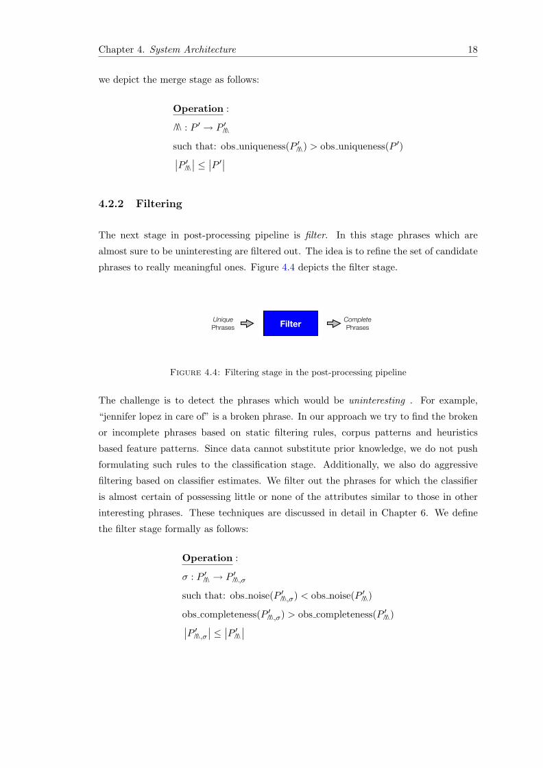
4.2.2 Filtering
The next stage in post-processing pipeline is filter. In this stage phrases which are
almost sure to be uninteresting are filtered out. The idea is to refine the set of candidate
phrases to really meaningful ones. Figure 4.4 depicts the filter stage.
Unique Phrases
CompletePhrasesFilter
Figure 4.4: Filtering stage in the post-processing pipeline
The challenge is to detect the phrases which would be uninteresting . For example,
“jennifer lopez in care of” is a broken phrase. In our approach we try to find the broken
or incomplete phrases based on static filtering rules, corpus patterns and heuristics
based feature patterns. Since data cannot substitute prior knowledge, we do not push
formulating such rules to the classification stage. Additionally, we also do aggressive
filtering based on classifier estimates. We filter out the phrases for which the classifier
is almost certain of possessing little or none of the attributes similar to those in other
interesting phrases. These techniques are discussed in detail in Chapter 6. We define
the filter stage formally as follows:
Operation :
σ : P ′! → P ′
!,σ
such that: obs noise(P ′!,σ) < obs noise(P ′
!)
obs completeness(P ′!,σ) > obs completeness(P ′
!)∣∣P ′!,σ∣∣ ≤ ∣∣P ′
!∣∣
Chapter 4. System Architecture 19
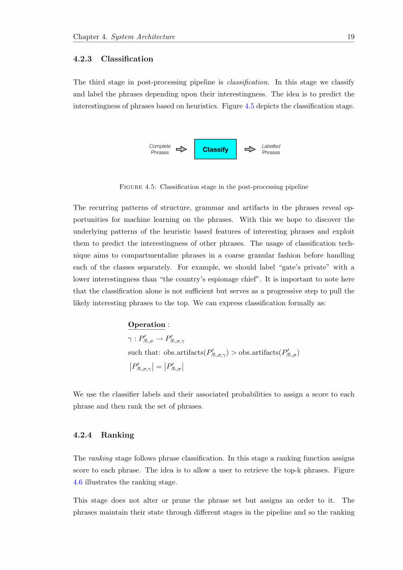
4.2.3 Classification
The third stage in post-processing pipeline is classification. In this stage we classify
and label the phrases depending upon their interestingness. The idea is to predict the
interestingness of phrases based on heuristics. Figure 4.5 depicts the classification stage.
Complete Phrases
LabelledPhrasesClassify
Figure 4.5: Classification stage in the post-processing pipeline
The recurring patterns of structure, grammar and artifacts in the phrases reveal op-
portunities for machine learning on the phrases. With this we hope to discover the
underlying patterns of the heuristic based features of interesting phrases and exploit
them to predict the interestingness of other phrases. The usage of classification tech-
nique aims to compartmentalize phrases in a coarse granular fashion before handling
each of the classes separately. For example, we should label “gate’s private” with a
lower interestingness than “the country’s espionage chief”. It is important to note here
that the classification alone is not sufficient but serves as a progressive step to pull the
likely interesting phrases to the top. We can express classification formally as:
Operation :
γ : P ′!,σ → P ′
!,σ,γ
such that: obs artifacts(P ′!,σ,γ) > obs artifacts(P ′
!,σ)∣∣P ′!,σ,γ
∣∣ =∣∣P ′
!,σ∣∣
We use the classifier labels and their associated probabilities to assign a score to each
phrase and then rank the set of phrases.
4.2.4 Ranking
The ranking stage follows phrase classification. In this stage a ranking function assigns
score to each phrase. The idea is to allow a user to retrieve the top-k phrases. Figure
4.6 illustrates the ranking stage.
This stage does not alter or prune the phrase set but assigns an order to it. The
phrases maintain their state through different stages in the pipeline and so the ranking

Chapter 4. System Architecture 20
Classified Phrases
RankedPhrasesRank
Figure 4.6: Ranking stage in the post-processing pipeline
function can make use of the intermediate processing results. This stage quantifies the
interestingness of a phrase. This allows us to compare phrases amongst each other. We
can formulate ranking stage as:
Operation :
µ : P ′!,σ,γ → P ′
!,σ,γ,µ
such that: obs order(P ′!,σ,γ,µ) > obs order(P ′
!,σ,γ)∣∣P ′!,σ,γ,µ
∣∣ =∣∣P ′
!,σ,γ∣∣
4.2.5 Grouping
Finally, the last stage in the post-processing pipeline is grouping. This stage attempts
to create groups of the phrases. Figure 4.7 illustrates the grouping stage.
Ranked Phrases
QualityPhrasesGroup
Figure 4.7: Grouping stage in the post-processing pipeline
Though the ranking stage produces phrases in a sorted list fashion, the result listings
tend to be quite large in practical systems. Thus, it becomes difficult for a user to
navigate through all the phrases in the result list. Also, our merging techniques do not
capture the topics of the phrases. Hence, many interesting phrases might be on the same
topic or theme. A user may not be interested in one particular topic. Since our system
does takes into account the interest of each user, it becomes imperative to bring out a
diverse set of interesting phrases. Hence, grouping becomes important for dynamic drill

Chapter 4. System Architecture 21
down by a user. We can model grouping as follows:
Operation :
Γ : P ′!,σ,γ,µ → P ′
!,σ,γ,µ,Γ
such that: obs diversity(P ′!,σ,γ,µ,Γ) > obs diversity(P ′
!,σ,γ,µ)∣∣P ′!,σ,γ,µ,Γ
∣∣ =∣∣P ′
!,σ,γ,µ∣∣
4.3 User Interface
Apart from an effective post-processing, the phrase mining system must also have an
intuitive user interface. The evolution of the Internet in the past decade has made the
Google style web interfaces a must for most document related retrieval systems. The
users are able to relate to it better and faster. Such interfaces usually allow users to
enter query keywords as text input and see matching documents ranked by relevance
below. Figure 4.8 shows a screenshot of the phrase mining user interface developed
by Sven Obser and Tobias Leidinger [25, 30]. This interface follows the Google style
convention and additionally displays interesting phrases from the retrieved documents
on the right hand side. By default, the phrase tab displays top-10 interesting phrases
but we can customize it for more phrases or for group-wise display. Similar to document
result pages’ navigation, the next page of the phrase results can be navigated further.
Since the post-processing pipeline has stages like merging and filtering, it makes sense
to take a considerable number of phrases in the candidate set. A large candidate set
of phrases produces better post-processed phrases. This also serves the dual purpose of
caching. When a user requests only top-10 phrases, the remaining phrases are cached
in the main memory. When the user requests next-10, they are readily available.
In addition to single queries, this interface also supports differential queries to compare
document and phrase results from two queries. For example, a user might be interested
in comparing documents and phrases for “George Bush” and “Barack Obama”. The
important thing to note here is that the underlying post-processing pipeline remains
the same, processing phrases for both the queries separately. This, however, causes the
system to respond quite slow. A possible way to alleviate this problem is to present
intermediate results to the user and keep on updating them as phrases pass though the
different stages in the pipeline. The interface presents OLAP style query results on
similar lines.

Chapter 4. System Architecture 22
Figure 4.8: Screenshot of phrase mining user interface
4.4 Conclusion
Interesting phrases are complementary to the document results from a document re-
trieval system. Therefore, a user expects them to be concise and qualitatively rich. Our
system enables this by post-processing the phrases in a series of stages. The phrase
mining system is built on top of a conventional search engine and hence can be easily
added on top of any another document style information retrieval system. Our current
approach to phrase mining is a bit conservative in terms of interestingness decisiveness.
However, the system makes an effort to channel the results though an intuitive user in-
terface. Additionally, the real time systems need to meet the response time constraints
of a few seconds. Therefore, the phrase mining capabilities should not add too much of
latency overhead.
Finally, interestingness also carries quite a bit of subjectivity. The final set of phrases are
still candidate phrases from a user’s perspective but with a higher confidence of being
interesting. Therefore, next step would be to take the user interest into account. The
next level systems should have interactive user interfaces with user sessions capturing
the user intent and interests to refine down the phrases to targeted ones.

Chapter 5
Merge Strategies
This chapter describes the phrase merging stage in the post-processing pipeline. The
merging stage aggregates all similar phrases with a two fold objective: (1) render unique-
ness by discarding complementary phrases and (2) enrich result set by merging supple-
mentary phrases. The first objective cleans the phrase set from near duplicate phrases
while the second objective produces more meaningful phrases. We try to be conservative
in our merge strategies. First we merge the phrases based on a partial or a complete
overlap between them. Next we take the edit distance as a simple yet effective measure
of string similarity and apply it to the phrases to do approximate merging of the phrases.
5.1 Exact Merge
Figure 5.1 depicts the internal pipeline of the merge stage. This stage looks for a prefix or
a suffix overlap between two phrases. The overlap here means a string match. Depending
upon the overlap we consider the following four cases:
1. The two phrases have a complete overlap of words i.e they are exact duplicates.
2. One phrase is the prefix of the other i.e. it is left contained.
3. One phrase is the suffix of the other i.e. it is right contained.
4. The two phrases have an overlapping prefix and suffix respectively.
The first case of exact duplicates is trivial to handle. We describe the second, third and
fourth cases in detail in the following sub-sections. Figure 5.1 indicates them as the first
three sub-stage in the internal pipeline. Currently, we do not consider merging phrases
which are contained in the middle of other phrases.
23

Chapter 5. Merge Strategies 24
PrefixMerge
Candidate Phrases
MergedPhrases
SuffixMerge
Prefix-SuffixMerge
SynonymMerge
Stop-WordMerge
Exact Merge Approximate Merge
MergeCandidate Phrases
QualityPhrasesFilter Rank GroupClassify
Figure 5.1: Merging strategies in the post-processing pipeline
5.1.1 Prefix Merge
The core idea of the prefix merge is to merge phrases which are prefixes of other phrases
in the set of candidate phrases. In other words we detect and ignore phrases which
are subsumed as prefixes in other phrases. We can do so because smaller subsumed
phrases typically tend to be broken. Or, they are incomplete and contain duplicated
information. For example, consider the phrases in Table 5.1.
1 those who shall live in sin2 those who shall live in sin shall die in sin3 those who shall live in4 those who
Table 5.1: Example of prefix merge
The second phrase in the above table is the most complete and hence the most interesting
among the four given phrases. Although the first phrase makes sense, it is more complete
and interesting when merged into the second phrase. The third phrase is broken in the
end and therefore we can safely merge it. Here, the fourth phrase is an example of noise
phrases created as a result of brute force sliding window and simply gets ignored. Hence,
a prefix merge of the four sentences shown in Table 5.1 produces “those who shall live
in sin shall die in sin” as the most comprehensive phrase.
Algorithm Overview: Algorithm 5.1 presents the pseudo code of the prefix merge
illustrated above. It takes candidate set of phrases as input. We first sort the candidate
phrases lexicographically in line 1. Next, we initialize a set of merged phrases to empty
set (line 2). We maintain the largest prefix seen so far and initialize it (line 3). We also
maintain a count of the number of phrases that get merged (line 4). We iterate over

Chapter 5. Merge Strategies 25
Algorithm 5.1: prefixMergeinput : Set of candidate phrasesoutput: Set of merged phrases
List<Phrase>sortedPhrases←− Sort(phrases,LexicographicComparator);1
Set mergedPhrases←− ∅;2
String prefix←− “”;3
Integer mergeCount←− 0;4
foreach Phrase p in sortedPhrases do5
if startsWith(prefix,p) then6
// case 1: prefix contains the phrase7
mergeCount←− mergeCount+ 1;8
else9
if startsWith(p,prefix) then10
// case 2: phrase contains the prefix11
mergeCount←− mergeCount+ 1;12
else13
// case 3: phrase totally different from the prefix14
mergedPhrases←− mergedPhrases ∪ {prefix};15
end16
prefix←− phrase;17
end18
end19
mergedPhrases←− mergedPhrases ∪ {prefix};20
return mergedPhrases;21
each phrase in the sorted list of phrases (line 5) and ignore it, if it has the same prefix
as seen so far (line 6-9). Otherwise, either the phrase contains the prefix seen so far
(line 10-12) or it is a completely new phrase, in which case we add the prefix seen so far
to the set of merged phrases (line 13-16). In both these cases we set the prefix seen so
far to the new phrase (line 17). Finally, we add the last remaining prefix to the set of
merged phrases (line 20). The algorithm returns the set of merged phrases (line 21).
Analysis: We do the sorting in prefix merge using quick sort and hence it has a time
complexity ofO(nlogn), where n is the number of phrases in the input candidate set. The
merge operation is a single scan operation, wherein we maintain the most comprehensive
phrase seen so far. As soon as we encounter a totally new phrase, we add the previous
most comprehensive phrase to the set of merged phrases. Thus the time complexity of
the prefix merge operation is O(n). The sorting prior to merging helps to avoid the time
complexity getting into quadratic terms.

Chapter 5. Merge Strategies 26
5.1.2 Suffix Merge
Suffix merge is the next merge variant within the merge post-processing stage. Similar
to prefix merge, the basic idea is to merge phrases which are suffixes of other phrases in
the set of candidate phrases i.e. we detect and ignore the phrases which are subsumed
as suffixes in other phrases. The intuition is that the phrases which start in the middle
of a sentence make no sense or contain duplicate information. For example, consider the
phrases in Table 5.2:
1 the iraq clamor2 bush, blair and the iraq clamor3 and the iraq clamor4 blair and the iraq clamor
Table 5.2: Example of suffix merge
Again, the second phrase in the above table is the most complete and hence most
interesting amongst the given four phrases. Though the first phrase also makes sense
but it is more comprehensible and interesting when we merge it into the second phrase.
The third phrase starts in the middle and therefore we can safely merge it. The fourth
phrase looks complete as well as interesting but it carries only one of the two person
named entities in the phrase. Such half information could be unpleasant or undesirable
to various sensitivities. Hence, suffix merge of the four sentences shown in Table 5.2
produces “bush, blair and the iraq clamor” as the most comprehensive phrase.
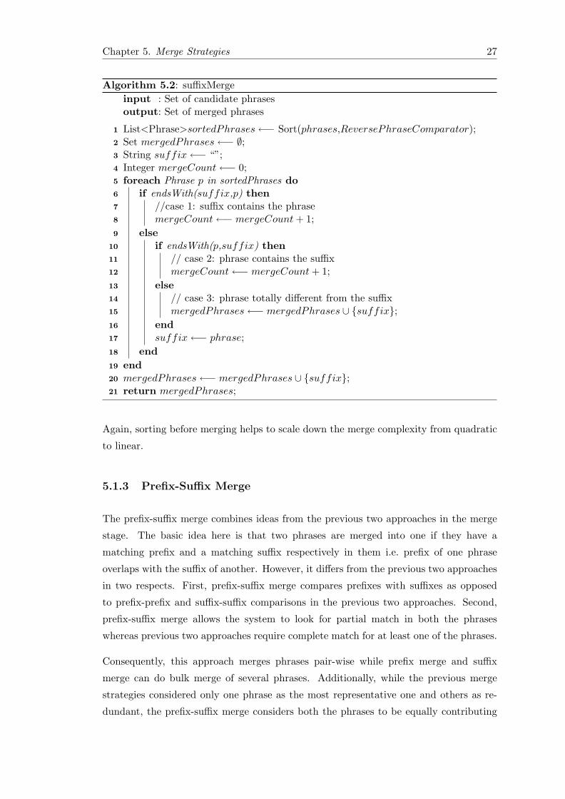
Algorithm Overview: Algorithm 5.2 details the pseudo code of the suffix merge
algorithm as discussed in the above example. Since here we are merging phrases based
on common suffixes, we need to sort the reverse phrases. Line 1 sorts the input set of
candidate phrases using ReversePhraseComparator. This comparator reverses the two
phrases strings before comparing them lexicographically. Rest of the algorithm is similar
to prefix merge. Only difference is that we maintain the largest suffix seen so far while
iterating over the phrases in the candidate set.
Analysis: The major difference in the suffix merge from the prefix merge algorithm
is the the phrase comparator used while sorting. Additionally, to check for subsuming
phrases we check for endsWith instead of startsWith. Similar to that in the prefix merge,
the suffix merge also sorts the phrases using quick sort and has the time complexity of
O(nlogn), where n is the number of phrases in the input candidate set. Since the length
of each phrase is very small as compared to the number of phrases in the candidate set,
we neglect the time taken to reverse the phrases. The merge operation on sorted lists
is again linear, i.e. O(n), with respect to the number of phrases in the candidate set.
Chapter 5. Merge Strategies 27
Algorithm 5.2: suffixMergeinput : Set of candidate phrasesoutput: Set of merged phrases
List<Phrase>sortedPhrases←− Sort(phrases,ReversePhraseComparator);1
Set mergedPhrases←− ∅;2
String suffix←− “”;3
Integer mergeCount←− 0;4
foreach Phrase p in sortedPhrases do5
if endsWith(suffix,p) then6
//case 1: suffix contains the phrase7
mergeCount←− mergeCount+ 1;8
else9
if endsWith(p,suffix) then10
// case 2: phrase contains the suffix11
mergeCount←− mergeCount+ 1;12
else13
// case 3: phrase totally different from the suffix14
mergedPhrases←− mergedPhrases ∪ {suffix};15
end16
suffix←− phrase;17
end18
end19
mergedPhrases←− mergedPhrases ∪ {suffix};20
return mergedPhrases;21
Again, sorting before merging helps to scale down the merge complexity from quadratic
to linear.
5.1.3 Prefix-Suffix Merge
The prefix-suffix merge combines ideas from the previous two approaches in the merge
stage. The basic idea here is that two phrases are merged into one if they have a
matching prefix and a matching suffix respectively in them i.e. prefix of one phrase
overlaps with the suffix of another. However, it differs from the previous two approaches
in two respects. First, prefix-suffix merge compares prefixes with suffixes as opposed
to prefix-prefix and suffix-suffix comparisons in the previous two approaches. Second,
prefix-suffix merge allows the system to look for partial match in both the phrases
whereas previous two approaches require complete match for at least one of the phrases.
Consequently, this approach merges phrases pair-wise while prefix merge and suffix
merge can do bulk merge of several phrases. Additionally, while the previous merge
strategies considered only one phrase as the most representative one and others as re-
dundant, the prefix-suffix merge considers both the phrases to be equally contributing
Chapter 5. Merge Strategies 28
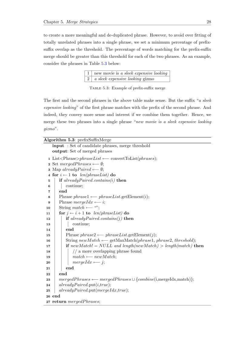
to create a more meaningful and de-duplicated phrase. However, to avoid over fitting of
totally unrelated phrases into a single phrase, we set a minimum percentage of prefix-
suffix overlap as the threshold. The percentage of words matching for the prefix-suffix
merge should be greater than this threshold for each of the two phrases. As an example,
consider the phrases in Table 5.3 below:
1 new movie is a sleek expensive looking2 a sleek expensive looking gizmo
Table 5.3: Example of prefix-suffix merge
The first and the second phrases in the above table make sense. But the suffix “a sleek
expensive looking” of the first phrase matches with the prefix of the second phrase. And
indeed, they convey more sense and interest if we combine them together. Hence, we
merge these two phrases into a single phrase “new movie is a sleek expensive looking
gizmo”.
Algorithm 5.3: prefixSuffixMergeinput : Set of candidate phrases, merge thresholdoutput: Set of merged phrases
List<Phrase>phraseList←− convertToList(phrases);1
Set mergedPhrases←− ∅;2
Map alreadyPaired←− ∅;3
for i ← 1 to len(phraseList) do4
if alreadyPaired.contains(i) then5
continue;6
end7
Phrase phrase1←− phraseList.getElement(i);8
Phrase mergeIdx←− i;9
String match←− “”;10
for j ← i+ 1 to len(phraseList) do11
if alreadyPaired.contains(j) then12
continue;13
end14
Phrase phrase2←− phraseList.getElement(j);15
String newMatch←− getMaxMatch(phrase1, phrase2, threshold);16
if newMatch! = NULL and length(newMatch) > length(match) then17
// a more overlapping phrase found18
match←− newMatch;19
mergeIdx←− j;20
end21
end22
mergedPhrases←− mergedPhrases ∪ {combine(i,mergeIdx,match)};23
alreadyPaired.put(i,true);24
alreadyPaired.put(mergeIdx,true);25
end26
return mergedPhrases;27

Chapter 5. Merge Strategies 29
Algorithm Overview: Algorithm 5.3 sketches the prefix-suffix merge. Input to the
algorithm are a set of candidate phrases and the overlap threshold parameter. Since
we merge the phrases pair-wise, we do not consider the phrases already merged in the
current iteration again. Line 1 converts the set of phrases to a list. Next, we initialize
the set of merged phrases to empty (line 2). We maintain a map to keep track of
the phrases already being paired in the current iteration (line 3). We iterate over all
the indices of the phrases in the phrase list (line 4). The algorithm skips the indices
whose corresponding phrases have already been paired (line 5-7). We fetch the phrase
corresponding to the current index as phrase1 (line 8). MergeIdx maintains the index
of the phrase most overlapping with phrase1 (line 9) and match maintains the overlap
between the two (line 10). Next, we iterate over all remaining phrases in the phrase
list to find the most overlapping phrase with phrase1 (line 11). Again, we skip the
indices whose corresponding phrases have already been paired (line 12-14). Otherwise,
we compute the maximum overlapping match between the current phrase (phrase2 in
line 15) and phrase1 (line 16). We set the maximum overlap as “null” if it is below
the threshold. We update the merge index and match if the maximum overlap thus
computed is bigger than the match seen so far (line 17-21). We merge phrase1 with the
maximum overlapping phrase and add the merged phrase to the set of merged phrases
(line 23). We add the index of phrase1 and mergeIdx to the map of already paired indices
(line 24-25). After merging phrases pair-wise in this fashion, the algorithm returns the
set of merged phrases as output.
In the above algorithm, getMaxMatch() finds the maximum prefix-suffix match between
two phrases. This can be done by first trying to match the maximum prefix of the first
phrase which overlaps with the suffix of the second phrase and then doing the other way
round. It can then return the maximum of the two matches.
Analysis: The sliding window that we use for phrase generation affects the size of the
index. A larger sliding window allows phrases of several lengths and hence produce
many more phrases. For this purpose, we fix the minimum and maximum lengths of the
phrases at the index creation time. But the prefix-suffix merge can create phrases larger
than the maximum phrase length. However, by suitably setting the minimum overlap
parameter (threshold) we can limit the maximum phrase length overshoot. For e.g. the
minimum overlap threshold of 60% can increase the phrase length by at most 40%.
The prefix-suffix merge algorithm merges the phrases pair-wise and hence cannot merge
multiple phrases in one pass. Also, due to the minimum overlap threshold criteria many
phrases may not qualify for merge initially but may qualify later. Therefore we do
multiple passes of the above algorithm as long as the set of merged phrases set keeps
on shrinking. Each recursive call to the prefix-sufix merge tries to find the maximum

Chapter 5. Merge Strategies 30
overlapping phrases satisfying the threshold criteria. Each pass however is a brute force
approach to compare a given phrase with all other phrases. This is unavoidable because
unlike the previous two merge techniques, this technique considers both prefixes and
suffixes at the same time. Consequently, the sorting of phrases is not possible in this
stage. The brute force comparison of every phrase with every other phrase renders the
time complexity as O(n2), where n is the number of phrases. However, we push the
prefix-suffix merge to the end of the internal merge pipeline i.e we apply it as late as
possible. This helps in reducing the size of the set of candidate phrases as much as
possible from the previous stages.
Finally, note that since the prefix-suffix merge procedure merges phrase having par-
tial match, this technique can produce unintended results. It can merge phrases from
different documents and different contexts. The choice of the minimum matching thresh-
old becomes crucial. A lower threshold value may greatly reduce the set of candidate
phrases but runs the risk of unintended merges. A higher threshold value may be too
conservative to have any effect.
5.2 Approximate Merge
So far we have considered subsuming or overlapping phrases and merged them. But many
times phrases have similar, though not exact, words, structure and even information.
This makes them repetitive and hence redundant e.g. “Angela Merkel Chancellor” and
“Angela Merkel the Chancellor”. It is therefore important to merge phrases based on an
approximate match as well. By approximate match we mean that two phrases may not
contain a common continuous sequence of words but rather a sequence of almost similar
words. We describe and discuss edit distance based string similarity techniques below.
Edit distance Measures: Edit distance is defined as the minimum number of editing
operations like insert, delete etc., needed to transform one string into the other. Or,
in other words how many edit operations away is one string from the other. Different
edit distances have been proposed. Hamming distance [21], for example, measures the
number of substitutions required for equal length strings to inter-convert. Naturally,
hamming distance is suited for comparing similarities only between equal length strings.
Extending this, Levenshtein distance [27] considers insert, delete or substitute operations
to measure edit distance. Damerau-Levenshtein distance [17] goes one step further by
including transpose operations while computing the minimum number of edit operations.
However, research literature typically defines these distance measures for character level
edit operations and they are typically used for spell check and similar operations. The
Chapter 5. Merge Strategies 31
character level editing may not be the best approach to find similarities between the
phrases. Below we discuss the application of edit distance to phrases.
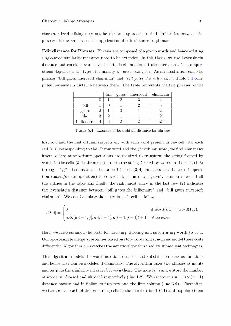
Edit distance for Phrases: Phrases are composed of a group words and hence existing
single-word similarity measures need to be extended. In this thesis, we use Levenshtein
distance and consider word level insert, delete and substitute operations. These oper-
ations depend on the type of similarity we are looking for. As an illustration consider
phrases “bill gates microsoft chairman” and “bill gates the billionaire”. Table 5.4 com-
putes Levenshtein distance between them. The table represents the two phrases as the
bill gates microsoft chairman0 1 2 3 4
bill 1 0 1 2 3gates 2 1 0 1 2the 3 2 1 1 2
billionaire 4 3 2 2 2
Table 5.4: Example of levenshtein distance for phrases
first row and the first column respectively with each word present in one cell. For each
cell (i, j) corresponding to the ith row word and the jth column word, we find how many
insert, delete or substitute operations are required to transform the string formed by
words in the cells (3, 1) through (i, 1) into the string formed by words in the cells (1, 3)
through (1, j). For instance, the value 1 in cell (3, 4) indicates that it takes 1 opera-
tion (insert/delete operation) to convert “bill” into “bill gates”. Similarly, we fill all
the entries in the table and finally the right most entry in the last row (2) indicates
the levenshtein distance between “bill gates the billionaire” and “bill gates microsoft
chairman”. We can formulate the entry in each cell as follows:
d[i, j] =
0 if word(i, 1) = word(1, j),
min(d[i− 1, j], d[i, j − 1], d[i− 1, j − 1]) + 1 otherwise.
Here, we have assumed the costs for inserting, deleting and substituting words to be 1.
Our approximate merge approaches based on stop-words and synonyms model these costs
differently. Algorithm 5.4 sketches the generic algorithm used by subsequent techniques.
This algorithm models the word insertion, deletion and substitution costs as functions
and hence they can be modeled dynamically. The algorithm takes two phrases as inputs
and outputs the similarity measure between them. The indices m and n store the number
of words in phrase1 and phrase2 respectively (line 1-2). We create an (m+ 1)× (n+ 1)
distance matrix and initialize its first row and the first column (line 3-9). Thereafter,
we iterate over each of the remaining cells in the matrix (line 10-11) and populate them

Chapter 5. Merge Strategies 32
Algorithm 5.4: approxMergeinput : phrase1, phrase2output: similarity
Set m←− wordCount(phrase1);1
Set n←− wordCount(phrase2);2
Set d←− matrix[m+ 1, n+ 1];3
for i← 0 to m do4
Set d[i, 0]←− i;5
end6
for j ← 0 to n do7
Set d[0, j]←− j;8
end9
for i← 1 to m do10
for j ← 1 to n do11
Set insertDistance←− d[i− 1, j] + insertCost(getWord(phrase1,i− 1));12
Set deleteDistance←− d[i, j − 1] + deleteCost(getWord(phrase2,j − 1));13
Set substituteDistance←− d[i− 1, j − 1] +14
substituteCost(getWord(phrase1,i− 1), getWord(phrase2,j − 1));Set d[i, j]←− min(insertDistance, deleteDistance, substituteDistance);15
end16
end17
return d[i, j];18
with the minimum of insertion, deletion and substitution costs (line 12-15). We leave the
definition of these costs for specific implementation. The following sub-sections discuss
two specific implementation of this algorithm.
5.2.1 Stop-Word Merge
The stop-word merge is a variant of Levenshtein distance wherein insertion or deletion
of stop-words have very less cost as compared to other words. Typically, we assign
fractional weights to the stop-word insertion/deletion and integral weights to the inser-
tion/deletion of other words. For instance, we can assign the stop-word insertion/dele-
tion cost to 0.1 if we can ignore up to 10 stop words in a phrase. The cost for substitution
is 0 in case two words are equal and 1 otherwise. We write the insert/delete and the
substitute cost functions as follows:
InsertOrDeleteCost (Word) =
0.1 if Word is stop-word
1 otherwise.

Chapter 5. Merge Strategies 33
SubstituteCost (Word1,Word2) =
0 if Word1 = Word2
1 otherwise.
With such a weight assignment an edit distance less than 1 would indicate at most 10
stop-word insert/delete operations. All bigger edit distances would represent one or
more non-stop word insertions/deletions, greater than 10 stop-word insertions/deletions
or substitution operations. We consider phrases having Levenshtein edit distance be-
tween them smaller than 1.0 as similar. For example, Table 5.5 shows the edit distance
computed between “angela merkel chancellor” and “angela merkel the chancellor”. Since
the phrases differ only in the stop-word “the”, the edit distance between them comes
out to be 0.1 (lower right cell). Hence the two phrases are similar.
angela merkel the chancellor0 1 2 3 4
angela 1 0 1 1.1 2.1merkel 2 1 0 0.1 1.1
chancellor 3 2 1 1 0.1
Table 5.5: Example of stop-word merge for phrases
We find the similar phrases in this fashion in our set of candidate phrases and merge
them. Note, that this method finds the pairwise similar phrases. Hence, similar to
prefix-suffix merge in algorithm 5.3 we run nested loops over all the phrases to find the
most similar pair of phrases and merge them. In many cases stop-words are not the
most desirable features, while merging the two phrases we keep the shorter of the two
phrases and discard the other one. For stop-words lookup we use a stop-word list [9]
maintained by the Linguistics Department at the University of Glasgow.
Analysis: The merge operation is pairwise and doubly nested over the set of candidate
phrases, therefore the time complexity is O(n2), similar to prefix-suffix merge. The stop-
words list that we use contains 319 stop-words and ca be looked up using a hash map.
Depending on the maximum number of stop-words which we can tolerate in each phrase,
we adjust the fractional cost assigned to insert/delete of stop-word. Further, instead of
assigning fixed costs to stop-words and non stop-words, we can assign costs inversely
proportional to the individual term frequencies. This would imply that frequent terms,
which are more likely to be stop-words, will have very small insert/delete costs.
5.2.2 Synonym Merge
Synonym merge uses another variant of Levenshtein distance wherein substitution of
synonyms words carries lesser weight compared to substitutions of other words. We

Chapter 5. Merge Strategies 34
assign zero cost to substitution of synonyms and integral weight to all other edit oper-
ations. Effectively, we relax the equality condition for words and consider synonyms as
equal. We represent the insert/delete and substitute cost functions as follows:
InsertOrDeleteCost (Word) = 1
SubstituteCost (Word1,Word2) =
0 if Word1 = Word2 or Word1 synonym of Word2
1 otherwise.
Again, we consider phrases having only synonym substitution operations as similar and
merge them. As an example, Table 5.6 shows the computation of edit distance between
“google announced quarterly results” and “google declared quarterly results” using such
a substitution cost function. The final edit distance between the two phrases is 0 (lower
right cell).
google announced quarterly results0 1 2 3 4
google 1 0 1 2 3declared 2 1 0 1 2quarterly 3 2 1 0 1
results 4 3 2 1 0
Table 5.6: Example of synonym merge for phrases
Similar to the stop-word merge, the synonym merge is a pair-wise merge. Hence we need
to iterate in nested loops over candidate phrases to merge all phrases. Since the similar
phrases differ only in synonymy, in order to merge them we discard one of the phrases
and keep the other one. We use the open source lexical english database WordNet [13]
to lookup the word synonyms. We fetch sets of synonyms, called synsets, for one of the
word and match the other word with each item in the synsets. If we find a match then
we consider the two words as synonyms. Otherwise, we fetch synonym sets of the other
word and match the first word against it. If still we do not find a match then the two
words are not considered as synonyms.
Analysis: Similar to the stop-word merge, the synonym merge being pair-wise, we
need nested loops for all possible merges. The time complexity of the merge operation
is O(n2), where n is the number of candidate phrases. However, synonym lookup is
expensive. WordNet 3.0 contains over 155,000 words with over 117,000 synsets and
hence locating a word in the synsets of the other is an expensive task. Once we detect
two phrases as similar, the question is how to merge them. Currently, we take either
of the two phrases and discard the other. This may not be the best strategy. A better
approach could be to use the term frequencies and retain the phrases having rarer

Chapter 5. Merge Strategies 35
terms. Finally, as opposed to the previous merge strategies, synonym merge works for
a highly selective and rather rare pairs of phrases. Hence, the performance pay off for
the synonym merge is low and its usage should be judicious.
5.2.3 Other Merges
We can extend the approximate merge for phrases as illustrated in algorithm 5.4 to many
other notions of text similarity. One such example could be approximate merge based
on stemming. Many phrases have the same word stem but they differ morphologically.
It could make great sense to merge all such phrases having same word stems. Another
example could be the use of phonetics based similarity depending on the application and
document content type. For example, documents about music (with transliterated song
snippets) could be used for such a merge.
5.3 Conclusion
We merge phrases to unique-ify the candidate set. We presented merge strategies in
this chapter which aim at combining complementary phrases and discarding redundant
supplementary phrases. We can merge phrases by the exact merge or the approximate
merge algorithms. The approximate merge carries the risk of false positives i.e. we
may merge phrases which are not really similar. But our approaches of stop-word
and synonym merges are conservative to weed out really similar phrases. We can take
more fuzzy matches into account depending upon the application requirements and
user preferences. The experiment section in Chapter 10 discusses the merging and
performance effectiveness of each of the merge strategies presented in this chapter.

36

Chapter 6
Filter Strategies
This chapter describes the filtering stage in the post-processing pipeline. The previous
merging stage produces unique phrases but many of them are not meaningful. The
filtering stage attempts to identify and filter out the phrases which could not possibly
make any sense to a user. The strategies presented in this chapter focus on the structural
and grammatical completeness of the phrases. Our phrase mining system filters out all
incomplete phrases broken in this sense.
6.1 Static Rule based filtering
Figure 6.1 depicts the filter stage and its sub-stages. The first three sub-stages are
static filters. Prior to post-processing, the phrases have been generated by the brute
force sliding window method. Hence, they are often cut in the middle at unexpected
positions in a sentence. This make them incomplete and hence incomprehensible to a
user. The large number of such malformed phrases need a filter for screening. Static
filters which are based on some pre-identified rules serve well for this purpose. Rules are
formed by looking at the data and generalizing over recurring patterns in the phrases.
As a consequence of filtering we incorporate all available prior knowledge about the data
and rule out the meaningless phrases. This helps in the classification stage which follows
next. The following sub-sections detail the three static filters based on the corpus, the
prefix-suffix information and parts-of-speech respectively.
6.1.1 Custom filter
The custom filter filters out the phrases based on static rules derived from the corpus. We
use custom the filter to weed out the corpus specific noise like advertisements, obituaries,
37
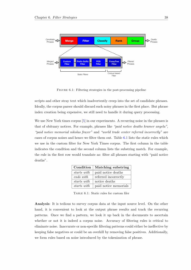
Chapter 6. Filter Strategies 38
Prefix-SuffixFilter
Merged Phrases
FilteredPhrases
POSFilter
FussyTreeFilter
Static FiltersCorpus based
Filter
Custom Filter
MergeCandidate Phrases
QualityPhrasesFilter Rank GroupClassify
Figure 6.1: Filtering strategies in the post-processing pipeline
scripts and other stray text which inadvertently creep into the set of candidate phrases.
Ideally, the corpus parser should discard such noisy phrases in the first place. But phrase
index creation being expensive, we still need to handle it during query processing.
We use New York times corpus [5] in our experiments. A recurring noise in the phrases is
that of obituary notices. For example, phrases like “paid notice deaths kramer angela”,
“paid notice memorial nikolas frazer” and “world trade center referred incorrectly” are
cases of corpus noises and hence we filter them out. Table 6.1 lists the static rules which
we use in the custom filter for New York Times corpus. The first column in the table
indicates the condition and the second column lists the substring match. For example,
the rule in the first row would translate as: filter all phrases starting with “paid notice
deaths”.
Condition Matching substringstarts with paid notice deathsends with referred incorrectlystarts with notice deathsstarts with paid notice memorials
Table 6.1: Static rules for custom filer
Analysis: It is tedious to survey corpus data at the input source level. On the other
hand, it is convenient to look at the output phrase results and track the recurring
patterns. Once we find a pattern, we look it up back in the documents to ascertain
whether or not it is indeed a corpus noise. Accuracy of filtering rules is critical to
eliminate noise. Inaccurate or non-specific filtering patterns could either be ineffective by
keeping false negatives or could be an overkill by removing false positives. Additionally,
we form rules based on noise introduced by the tokenization of phrase.

Chapter 6. Filter Strategies 39
6.1.2 Prefix/Suffix filter
The prefix/suffix filter matches patterns of prefixes or suffixes and statically removes
the matched ones. The difference here as compared to custom filter above is that the
filtered prefixes or suffixes are not characteristic of the corpus but apply quite in general.
For instance, looking at the candidate phrases over several queries, we noticed a large
number of phrases ending with articles (a, an, the) which do not make sense for the user.
While such phrases may still contain some interesting attributes, they do not make sense
on the whole e.g. “tsunami hit the”. Here note that we are not interested in dissecting
a phrase into smaller parts to extract the information. We treat a phrase as a whole
and do not consider any sub-part of it. Hence, the phrases ending with articles can be
safely filtered out with high confidence. The conjunctions (and, or) appearing in the
end of a phrase are also the indicators of incompleteness. Similarly, many other phrases
are pieces of sentences having broken second or third person speeches. For instance, a
phrase may contain “said” in the end and make little sense to a user. An example of a
prefix pattern is the “s” from possessive terms. Table 6.2 lists the static rules which we
have identified.
Condition Matching patternends with &ends with andends with orends with aends with anends with theends with saidstarts with s
Table 6.2: Static rules for prefix/suffix filter
Analysis: As in the custom filter, we need to craft the filtering rules carefully after rig-
orous skimming on representative phrases. Also, we should suitably adjust the tradeoff
between effective and over filtering. The single word patterns match a wide group of
phrases. This makes this filtering approach less conservative. Although this seems nec-
essary, we need to substantiate it by studying the drop in precision for a given query. We
present the results analyzing the effectiveness and the cost of these filtering techniques
in Chapter 10.

Chapter 6. Filter Strategies 40
6.1.3 Parts-of-Speech (POS) filter
The Parts-of-Speech (POS) filter makes use of the grammatical structure of a phrase to
decide whether or not to filter it. Certain sequences of parts-of-speech are strong indica-
tors of incomplete sentences. We attempt to identify such parts-of-speech sequences and
discard all the matching phrases. We form static filtering rules based on these sequences
and apply them to the dynamically retrieved phrase set. We could have made the pre-
fix/suffix filter in the previous sub-section redundant by incorporating the prefix/suffix
rules as parts-of-speech sequences. However, note that the parts-of-speech sequences
define a very generic set of rules which encompass a wider group of phrases. Due to this
lack of specificity in the POS filter, we first apply the more specific prefix/suffix filter
followed by a limited and universally applicable set of POS rules. These rules are framed
based on observation on the data over a range of representative queries. Finally, static
rules based filter, like POS filter, allows us to to eliminate the meaningless phrases. This
helps in the classification stage where we can train on better set of training phrases.
For the parts-of-speech tagging we use the Stanford Parts-Of-Speech Tagger [8]. We
tag each word in a phrase by its parts-of-speech. We tag the phrases on the fly during
query processing. However, the phrases being subpart of sentences, the tagger may not
be able to tag them accurately. A more comprehensive approach would be to tag the
phrases and store their tags in the phrase index itself. However, this would slow down
the index creation and inflate the index size. We discuss this idea in more detail in
Chapter 11. The Stanford Parts-Of-Speech Tagger uses the Penn Treebank tag-set [6]
for producing the tag outputs. It produces 36 different tags but we use 32 major ones
to be able to encode it in five bits. Hence, in this way up to six-term phrases could have
their tags encoded into a single integer. The bit packing of the parts-of-speech tag into
an integer helps save memory and disk space (for index level tagging) and also speed up
computation by allowing bitwise operations.
The POS sequences which we identify as patterns for filtering could be prefixes, suffixes
or contained in the phrases. Since the corpus parser tokenizes the phrases, which in our
case replaces all special symbols by a space character, we have to take care of possessive
forms of words. This is to make sure to treat the possessive word and the following
“s” as a single word. For instance, two of our static rules (sno. 9, 10) filters out the
phrases ending with the possessive forms of common or proper nouns. Table 6.3 lists
the rules used in our parts-of-speech filter. The second column in the table indicates
the matching condition (prefix, suffix, possessive ending). The third column contains
the parts-of-speech sequences in the Penn Treebank tag-set notation. The last column
in the table gives relevant examples.

Chapter 6. Filter Strategies 41
SNo. Condition POS pattern tags Example1 starts with VBZ is the major client2 ends with NN CC performances by leigh gable and3 ends with NN IN jennifer lopez in care of4 ends with NNS IN the graduates of5 ends with NN WP al hallak who6 ends with VBD DT lopez birdied the7 ends with IN DT studio comedies of the8 ends with DT JJ its protagonist has a great9 ends possessive with NN my father’s10 ends possessive with NNP barrack obama’s
Table 6.3: Static rules for parts-of-speech filtering
Table 6.4 lists the description and examples of the tags used in the above rules. The
complete list of description for all tags can be found at [7].
Tag Description ExamplesCC conjunction, co-
ordinating& and both but either et for less minus neither nor or plusso therefore times v. versus vs. whether yet
DT determiner an another any both each either many much nary neither nosome such that the them these this those ...
IN preposition orconjunction,subordinating
astride among uppon whether out inside pro despite onby throughout below within for towards near behind atoparound if like until below next into if beside ...
JJ adjective or nu-meral, ordinal
third ill-mannered pre-war regrettable oiled calamitous firstseparable ectoplasmic battery-powered participatory fourthstill-to-be-named multilingual multi-disciplinary ...
NN noun, common,singular or mass
common-carrier cabbage afghan shed thermostat investmentslide humour falloff slick wind hyena override ...
NNP noun, proper, sin-gular
Motown Venneboeger Czestochwa Ranzer Conchita Trum-plane Christos Oceanside Escobar Kreisler Sawyer CougarYvette Ervin ODI Darryl CTCA Shannon A.K.C. Meltex ...
NNS noun, common,plural
undergraduates scotches bric-a-brac products bodyguardsfacets coasts divestitures storehouses designs clubs fra-grances averages subjectivists apprehensions muses ...
VBD verb, past tense dipped pleaded swiped regummed soaked tidied convenedhalted registered cushioned exacted snubbed strode aimedadopted belied figgered speculated wore appreciated ...
VBZ verb, presenttense, 3rd personsingular
bases reconstructs marks mixes displeases seals carps weavessnatches slumps stretches authorizes smolders picturesemerges stockpiles seduces fizzes uses bolsters slaps ...
WP WH-pronoun that what whatever whatsoever which who whom whosoever
Table 6.4: Static rules for parts-of-speech filtering
Analysis: As opposed to custom and prefix/suffix filters, the parts-of-speech filter de-
fines the most generic set of static rules. Hence, we need to evaluate the drop in precision

Chapter 6. Filter Strategies 42
across this stage. The POS tagging at post-processing time could be a processing over-
head since the system is constrained with a few seconds of response time. Hence, we
need to consider the time latency and the tagging accuracy requirements of this filter.
Chapter 10 details the evaluation for POS filter. Additionally, by virtue of using POS
tagger, this filter is restricted by the POS tagging capabilities. For instance, it cannot be
applied on multi-lingual corpus or corpus having transliterated text because POS tagger
will not work on these. Also, the POS tagger assumes grammatically well formed text in
the corpus. This may not be the case for many real world data like social network forums
and discussions which are prevalent with abbreviations and other colloquial language.
Finally, the static filtering techniques can be used for index pruning by removing the
phrases which are consistently observed to be filtered out over a period of time. Chapter
11 discusses these optimizations in detail.
6.2 Corpus-based filtering
The filters discussed so far try to formulate rules applicable across all phrases. But
we can also learn from the corpus itself. Recurring patterns in the corpus could be
framed as rules applicable to a particular corpus. Based on the corpus, if we are sure
of a group of words occurring together in a sequence then they can be used to detect
incompleteness. Given a phrase we try to see if it can be extended in its suffix. The
information pieces in sentences are usually in their latter part. Hence, phrases which
are extensible in their suffixes with high confidence could indicate incompleteness. We
can store frequent phrases in the corpus in a tree like data structure (e.g. suffix tree).
We can then use it to deduce whether a given phrase can be safely extended in its suffix
or not. Below, we describe the usage of a variant of suffix tree in our application.
6.2.1 FussyTree filter
Arnab et al. [29] propose a technique for phrase prediction in auto-completion and user
assistive systems. The idea is similar to string suffix trees [28]. Their objective is to
predict and suggest the full phrase suffix as a user starts typing in the first few words.
To do so, they propose a variant of the pruned count suffix tree called FussyTree in which
each node represents a word. Additionally, the FussyTree contains only those phrases
which satisfy the notion of significance. A phrase “AB” is said to be significant if it
satisfies the following conditions:
• frequency : “AB” occurs at least τ times in the corpus.

Chapter 6. Filter Strategies 43
• co-occurence : Observed joint probability of “AB” is higher than that of indepen-
dent occurrences, i.e.
P (“AB”) > P (“A”)× P (“B”)
• comparability : Likelihood occurrence of “AB” is comparable to “A”, i.e. for z ≥ 1
P (“AB”) ≥ 1z× P (“A”)
• uniqueness : “AB” is more likely than “ABC” for every choice of “C”, i.e.
P (“AB”) ≥ y × P (“ABC”)
Above four conditions have τ, y and z as tuning parameters. All the phrases satisfying
these conditions are inserted into the FussyTree. Algorithms 6.1-6.4 shows the construc-
tion of FussyTree. The FussyTree method first constructs a pruned n-gram frequency
table and then builds the tree as the second step. The n-gram frequency table contains
frequencies of all phrases of length up to a maximum window size. Algorithm 6.1 out-
lines the frequency table construction. The algorithm parses the corpus (line 1-5) and
updates the frequency table for each phrase found within the sliding window. It then
prunes the overall frequency table based on the minimum threshold frequency.
Algorithm 6.1: buildFrequencyTableinput: maxTrainingWindowSize, threshold
foreach document in corpus do1
foreach sentence in document do2
for i← to maxTrainingWindowSize do3
//slide through with a window of size i4
foreach phrase in slidingWindow(sentence,i) do5
updateFrequencyTable(phrase);6
end7
end8
end9
end10
pruneFrequencyTable(threshold);11
The next step us to built the FussyTree using the frequency table constructed above.
Algorithm 6.2 shows the building stage. Again, the algorithm parses the corpus (line
1-3) and calls addPhrase() method for each phrase of length maxWindowSize. The
algorithm adds the phrase and its sub-phrases recursively in addPhrase().
Algorithm 6.3 shows the addPhrase() method. The algorithm iterates over all prefixes
of the phrase. It adds the prefix if it satisfies the frequency criteria. Each node in

Chapter 6. Filter Strategies 44
Algorithm 6.2: buildFussyTreeinput: corpus, maxWindowSize
foreach document in corpus do1
foreach sentence in document do2
foreach phrase in slidingWindow(sentence,maxWindowSize) do3
addPhrase(phrase);4
end5
end6
end7
the suffix tree contains the word and pointers to its parent and children for navigation.
Additionally, the nodes having the last word of a phrase also contain a flag indicating that
this particular access path is a phrase. For better compression and memory optimization,
we use integer term IDs for each term in the phrase to store in the tree nodes. Also, note
that as opposed to single-term suffix trees where each node stores a single character and
hence can have at most 26 children, the suffix tree nodes in our scenario contain words
and hence can have a considerably large fan out.
Algorithm 6.3: addPhraseinput: phrase
while phrase 6= {} do1
if isFrequent(phrase) then2
appendToTree(phrase);3
return ;4
end5
Set phrase←− removeRightmostWord(phrase);6
end7
To check whether a phrase is frequent or not, we look up all its sub-phrases of length
up to maxTrainingWindowSize into the frequency table (Algorithm 6.4). If any of
these sub-phrases is not present in the already pruned frequency table then we consider
the phrase as infrequent. This is in accordance to the definition of significance that we
defined earlier.
The FussyTree construction is CPU intensive. However, since it is based on the corpus,
it changes only when the corpus changes. Hence, we can extract and store the frequent
phrases with their corresponding frequencies in a serialized fashion on the external stor-
age. We load these significant phrases into the tree structure in main memory during
startup. This saves the frequency table construction and phrase significance detection
overheads during startup.
Once we have constructed and loaded the FussyTree into the memory, we can look
up incoming phrases for possible suffix completions. Starting from the root node, for

Chapter 6. Filter Strategies 45
Algorithm 6.4: isFrequentinput : phraseoutput: boolean
for i← 1 to maxTrainingWindowSize do1
//slide through with a window of size i2
foreach p in slidingWindow(phrase,i) do3
if not frequencyTableContains(p) then4
return false;5
end6
end7
return true;8
end9
every word in the phrase we traverse down the suffix tree until we locate the node
corresponding to the last word in the phrase. From this node, we do breath first search
through its children to find if there are any descendent nodes marked as phrase. In case
we find at least one such descendent, the phrase is deduced to have a complementing
suffix. However, no suffix extension is possible if we cannot find a corresponding node
at any level in the suffix tree.
Suffix completions to a phrase predicted in this fashion can be used to decide whether
to keep or discard the original phrase. While the original FussyTree paper tries to
find possible completions for auto-suggestion, we find probable completions for effec-
tive filtering. However, we need to adjust the tuning parameters to transform the
acceptability criteria into unacceptability criteria with high confidence. Arnab et al.
[29] deduce maxTrainingWindowSize as 8. But while they are looking for arbitrar-
ily long auto-completions, we are looking at relatively smaller phrases. So we choose
maxTrainingWindowSize as 3 i.e. we consider uni-grams, bi-grams and tri-grams while
constructing the frequency table. Similarly, the original work decides the frequency
threshold value of 4. In our case we are looking at rejection criteria, hence we take
a threshold value of 12. Finally, we also limit the maximum phrase length to 9 while
building the tree. This is done considering our phrase index contains only 2-5 word
phrases.
We use FussyTree constructed in such a manner to find possible suffix completions. In
case we find a completion, the FussyTree filter discards the corresponding phrase from
the set of candidate phrases. An example scenario of such filtering can be a phrase
ending with only a part of a named entity that is truncated in between. For instance,
if we have a text corpus containing documents on world travel then the FussyTree can
detect a phrase ending with “the great wall” to be extending to “the great wall of china”.

Chapter 6. Filter Strategies 46
Analysis: Though the FussyTree stores the phrases as integers, the size of the trie is
a major concern. Arnab et al. [29] experimented with just 53MB of data whereas the
New York Times corpus which we use is 12GB in size. We construct a sparse tree in
our experiments choosing 1 in every 100 documents uniformly. The resulting FussyTree
with the above mentioned significance constraints has 882, 749 phrases and has a size
of around 700MB. This could be a considerable overhead given that the tree needs
to be in memory during post-processing. Another issue could be the effectiveness of
this filtering approach. While the phrases which FussyTree filters out could be justified,
the ones left behind may still be contentious. We need to evaluate the payoff for the
complicated tree construction and maintenance. Finally, the sparsity of the FussyTree
(1 in 100 documents in our case) is a crucial parameter. For larger data sets, as in
our case, there is a trade-off between coverage and size of the FussyTree. Consequently,
many phrases might not find their end node in the FussyTree due to the lack of coverage
and not due to insignificance.
6.3 Conclusion
Our phrase mining system system uses static rule based, corpus based and dynamic
classification based filtering. Filtering is an effective way to utilize information observ-
able from the data and alleviate the overhead in subsequent stages. The downside,
though, is the tedious inspection of data and the possible risking of loosing the relevant
phrases. While formulating filtering rules, there is a trade-off between too loose (under-
specifying) and too strict (over-specifying) rules. We need to evaluate the trade-off using
experimental study. Chapter 10 presents experimental results on this.

Chapter 7
Phrase Classification
This chapter describes the phrase classification stage in our post-processing pipeline. The
filtering process discussed in the previous chapter is a best effort filter and the subsequent
phrase set still contains a mix of phrases ranging from most the interesting to not at all
meaningful ones. Interesting phrases have an underlying pattern of attributes or features
and we wish to uncover it. For this we first extract all heuristics based attributes or
features characterizing a phrase. Depending upon their features, the phrases are assigned
labels as per their interestingness, evaluated with reference to a pre-labelled data. We
discuss the various steps of phrase classification in this chapter. Later, we aggressively
filter the phrases which are obviously uninteresting based on the classifier probability
estimates for the class labels.
7.1 Feature Extraction
The first step to machine learning based classification is to extract features from the
data items to be classified. A feature is a prominent or a distinctive aspect, quality or
characteristic of the data. To be able to make the decision of assigning a particular label
to a data item, we need to extract all such prominent and distinctive aspects present
in the data item. The quality and accuracy of classification depends on the choice of
features and their effective extraction. The goal is to identify and extract the typical
features that really characterize the data items to be able to do precise classification.
Though a perfect set of features is desirable, getting the right features is a challenging
task. Once extracted, we express the features in numerical terms and arrange them in
the vector form, called the feature vector. This helps us in performing the subsequent
computations. Since the feature vector for every data item has the same number of
47

Chapter 7. Phrase Classification 48
dimensions, many of them could be sparse vectors i.e. many dimensions may have empty
or null values due to the lack of the corresponding feature in the data item.
Feature Extraction
Filtered Phrases
ClassifiedPhrases
Feature Selection
Label Prediction
MergeCandidate Phrases
QualityPhrasesFilter Rank GroupClassify
ThresholdFilter
Figure 7.1: Classification steps in the post-processing pipeline
Our phrase mining system extracts features and constructs feature vectors for each of
the phrases. These vectors are then used to classify the phrases into labels depending
upon their interestingness levels. We are extracting features on the fly and hence time
level guarantees must be adhered. We face several problems in feature extraction. One
particular problem is their short length of phrases. Another problem is the ad-hoc nature
of phrases as they have been clipped from anywhere in a sentence. This impedes the
extraction of much more rich set of features as many of the artifacts may get split or
terminated unexpectedly. Below we list the phrase features used in our phrase mining
system and we describe their extraction in detail:
1. Number Of Terms: Amongst different phrases, the length of a phrase may be an
indicator of its interestingness. So this feature simply counts the number of single
word terms present in the phrase.
2. First Term: Starting word of a phrase may be another indicator of phrase quality.
Certain standard starting words may be helpful in identifying good or bad phrases
in terms of quality. This features classifies first word in the phrase as a stop-word,
an article, a query term or any other word and assigns it the value of 1,2,3 or 4
respectively.
3. Last Term: This feature finds the type of the last word in the phrase as a stop-
word, an article, a query term or any other word and assigns it the value of 1,2,3
or 4 respectively.
4. Fresh Terms Ratio: By fresh terms we mean terms other than stop-words and those
present in the user query. The fresh terms may indicate additional information in

Chapter 7. Phrase Classification 49
a phrase. This feature value corresponds to the ratio of the number of fresh terms
and the total number of terms in the phrase. We take the ratio to normalize the
value. Since number of terms is a separate feature, normalized values would suit
better.
5. Possessive Terms Ratio: During inspection of the data we observe a lot of pos-
sessive terms like “principal’s”. Apart from indicating a noun or even a named
entity, some information related to that noun may also follow the possessive term.
This feature value corresponds to the ratio of the number of possessive terms and
the number of terms in the phrase.
6. Average Term Length: The lengths of the terms in a phrase is another characteris-
tic of the phrase. While smaller length words tend to be more like stop-words and
irrelevant, larger length words are more likely to be conveying some information.
This feature contains the average length of all terms in a phrase.
7. Maximum Term Length: The average of the term lengths may smooth out a char-
acteristically long word in a long phrase. Hence, we use another feature to capture
this spike in the term length. This feature value is set to the maximum term length
amongst all terms in the phrase.
8. Salutation Terms Ratio: The salutation terms address people and indicate the
subsequent partial or complete presence of named entities. Such phrases may
obviously be of interest. The salutation terms we look for are: “mr”, “mrs”,
“miss”, “master”, “lord”, “excellency”, “highness” and “majesty”. This feature
value contains the number of salutation terms normalized by the total number of
terms in the phrase.
9. Initial Terms Ratio: Many times the names of people, places and organizations
are abbreviated, called initials, to the first alphabets of the terms. Again, this
gives indication about a named entity being discussed. This feature value consists
the ratio of the number of initial terms found in the phrase and total number of
terms present in it.
10. Currency Symbols Ratio: The currency symbols indicate some quantifiable infor-
mation, which could be of interest. This feature value represents the number of
dollar symbols normalized by the number of terms in the phrase.
11. Numeric Terms Ratio: As pointed out in previous feature numerical terms are
significant artifact in a phrase. The numbers may denote time, money, or any
other measurable quantity. This feature represents the ratio of the number of
numerical terms to the total number of terms in a phrase.

Chapter 7. Phrase Classification 50
12. Query Terms Ratio: The presence of query terms indicates relevance. At the same
time phrases being small length texts, too many query terms in a phrase may not
leave the room for any additional information. Nevertheless, number of query
terms is an important feature in a phrase. As in previous features, this number is
normalized.
13. Stop Words Ratio: The phrases inundated with stop-words may have less infor-
mation content and consequently lower interestingness value. However, there are
counter examples like “to be or not to be” where the phrase is interesting despite
most of its words being stop-words. This is an one-off example and stop-words
usually do not add to the information of interest. This feature value corresponds
to the fraction of stop-word terms in a phrase.
14. Articles Ratio: The stop-words cover a wide range of words and hence may not
form patterns in interesting phrases. Articles (“a”, “an”, “the”) on the other hand
is a smaller set and can have some recurring pattern in the data. This feature value
contains the fraction of article terms in the phrase.
15. Named Person Entities: This feature uses a named entity recognizer to extract
the named entities in the phrase. We use the Stanford Named Entity Recognizer
to extract named entities. The entities can have multiple terms within a phrase.
This feature value represents the number of person named entities (for example
“Jim Carrey”) found in the phrase. We do not normalize the value here because
we expect phrases containing more named entities to be more interesting despite
being longer.
16. Named Location Entities: This feature value represents the number of location
named entities (for example “London”) found in the phrase.
17. Named Organization Entities: This feature value represents the number of orga-
nization named entities (for example “Saarland University”) found in the phrase.
18. Parts Of Speech First Term: The parts-of-speech of the terms in the phrase can
help us understand the nature, structure and correctness of the phrase. Addition-
ally, presence of nouns can indicate things of interest. Phrases being of variable
length, it is not possible to capture parts-of-speech of every term in a phrase as a
feature. However, we can capture parts-of-speech for the starting and the ending
terms, which are crucial. We use the parts-of-speech tags from Penn Treebank
tag-set [6] and represent them as integers between 0-31. This feature value is the
integer representation of the parts-of-speech of the first term in the phrase.
19. Parts Of Speech Second Term: This feature value is the integer representation of
the parts-of-speech of the second term in the phrase.

Chapter 7. Phrase Classification 51
20. Parts Of Speech Last Term: This feature represents the parts-of-speech of the last
term in the phrase.
21. Parts Of Speech Second Last Term: This feature represents the parts-of-speech of
the second last term in the phrase.
22. Parts Of Speech Third Last Term: This feature represents the parts-of-speech of
the third last term in the phrase.
23. Inverse Term Frequency First Term: The term frequencies are good indicators of
frequent or rare terms. Rarity is an element of surprise and hence highly likely
to be interesting. Since we compute the frequencies over the full corpus, they do
not have any local effects. Inverse term frequencies are frequencies represented in
inverse order such that frequent terms have smaller numbers and rare terms have
larger number. Again, since we cannot put inverse term frequencies of all terms
in a phrase as features, we consider the inverse term frequencies of starting and
ending terms as features. This feature represents the inverse term frequency of the
first term in the phrase.
24. Inverse Term Frequency Second Term: This feature value represents the inverse
term frequency of the second term in the phrase.
25. Inverse Term Frequency Last Term: This feature value represents the inverse term
frequency of the last term in the phrase.
26. Inverse Term Frequency Second Last Term: This feature value represents the
inverse term frequency of the second last term in the phrase.
27. Inverse Term Frequency Third Last Term: This feature value represents the inverse
term frequency of the third last term in the phrase. Since ending words are more
crucial we take one extra term frequency in the trailing part of the phrase.
28. Average Inverse Term Frequency : The inverse term frequencies of the beginning
and the ending terms in a phrase give term level insight. Similarly, an average
of the term frequencies over all terms can give an idea of the overall rarity of the
phrase. This feature value represents the average of inverse term frequencies of all
terms in the phrase.
29. Maximum Inverse Term Frequency : Sometimes there is only one very rare term
in a phrase, enough to make the whole phrase interesting. This feature captures
such a spike by representing the maximum inverse frequency amongst all terms in
the phrase.

Chapter 7. Phrase Classification 52
30. Minimum Inverse Term Frequency : Converse to the maximum inverse term fre-
quency, this features represents the minimum inverse term frequency among all
terms in the phrase.
As mentioned before, the short phrase length is a hindrance to extracting a much more
rich set of features. However, we can push down some feature extraction techniques to
the indexing stage. For instance, we can do parts-of-speech tagging and store the tags at
the indexing stage itself. This improves the accuracy of tagging as the tagger can work
on full sentences as opposed to an ad-hoc subset of it. Similarly, we can do named entity
extraction at the indexing level as well. These techniques, however, require considerable
pre-processing and storage at index time. We discuss these in more detail in Chapter
11.
More possibilities on extracting phrase features exist. So far we have only considered
statistics local to our corpus. We can also consider global statistics from web search
engines. We can count the occurrences of phrases on such systems and thereby compute
point-wise mutual information style measure. This can be considered as another feature
for the phrases. So far we have characterized desirable aspects in a phrase. We could
also characterize the non-desired facets of the phrases.
Another approach for a more exhaustive set of underlying features could be to first
cluster similar phrases dynamically and then extract features from the whole group of
phrases. The classifier will then assign labels to clusters as a whole. We can extract
much more relevant and quantity of features from such a dynamic cluster of phrases.
The challenge, however, lies first in forming the appropriate clusters and second in
aggregating the features values of all phrases in the same cluster. Additionally, very
small clusters may tend to over-specialize while too big clusters may become generic.
One might also think that in order to create the right clusters we need the right features
and so the problem becomes recursive. Another issue is to aggregate the feature values
for a cluster of phrases. Averaging them could produce a jaded and lesser distinctive
feature set. Still we can explore this idea as part of future work.
7.2 Feature Selection
Not all the features present in a feature set may be relevant for the classifier. Many
features are redundant and add to the noise. Additionally, large number of dimensions
(each feature being a separate dimension) makes classification computationally expen-
sive. Pruning down the feature set to the more relevant features makes the training and
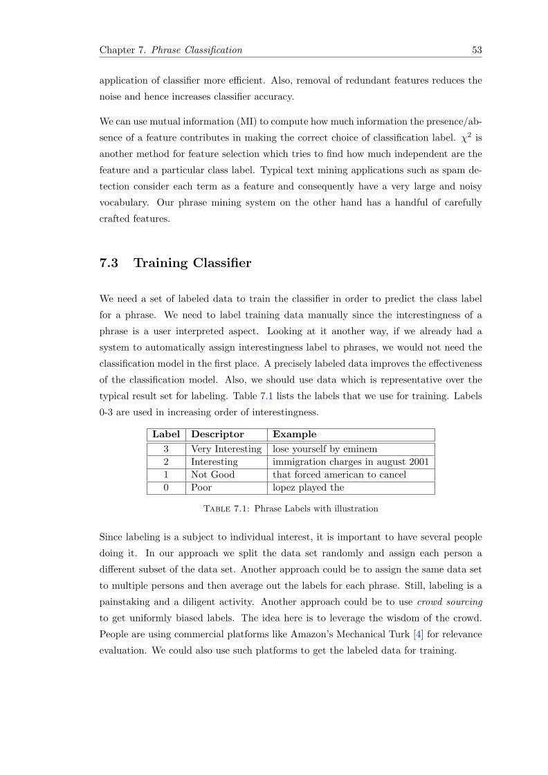
Chapter 7. Phrase Classification 53
application of classifier more efficient. Also, removal of redundant features reduces the
noise and hence increases classifier accuracy.
We can use mutual information (MI) to compute how much information the presence/ab-
sence of a feature contributes in making the correct choice of classification label. χ2 is
another method for feature selection which tries to find how much independent are the
feature and a particular class label. Typical text mining applications such as spam de-
tection consider each term as a feature and consequently have a very large and noisy
vocabulary. Our phrase mining system on the other hand has a handful of carefully
crafted features.
7.3 Training Classifier
We need a set of labeled data to train the classifier in order to predict the class label
for a phrase. We need to label training data manually since the interestingness of a
phrase is a user interpreted aspect. Looking at it another way, if we already had a
system to automatically assign interestingness label to phrases, we would not need the
classification model in the first place. A precisely labeled data improves the effectiveness
of the classification model. Also, we should use data which is representative over the
typical result set for labeling. Table 7.1 lists the labels that we use for training. Labels
0-3 are used in increasing order of interestingness.
Label Descriptor Example3 Very Interesting lose yourself by eminem2 Interesting immigration charges in august 20011 Not Good that forced american to cancel0 Poor lopez played the
Table 7.1: Phrase Labels with illustration
Since labeling is a subject to individual interest, it is important to have several people
doing it. In our approach we split the data set randomly and assign each person a
different subset of the data set. Another approach could be to assign the same data set
to multiple persons and then average out the labels for each phrase. Still, labeling is a
painstaking and a diligent activity. Another approach could be to use crowd sourcing
to get uniformly biased labels. The idea here is to leverage the wisdom of the crowd.
People are using commercial platforms like Amazon’s Mechanical Turk [4] for relevance
evaluation. We could also use such platforms to get the labeled data for training.

Chapter 7. Phrase Classification 54
7.4 Label Prediction (Classification)
Once we have the feature set and a training data, we can classify the phrases. Given a
data item, a classifier predicts the most likely class label for it. There is an important
distinction between classification and clustering which we need to clarify. Classification
is a supervised learning where we know the number of class labels before hand whereas
clustering is an unsupervised learning where we determine the number of class labels on
the fly. Consequently, classification requires labeled data as opposed to clustering.
One way to measure interestingness could be to combine the feature values, which are
already in numerical terms, in a linear fashion. The problem then boils down to learning
the weights of the features to be combined in the linear fashion. This is considered a
linear regression problem. A classifier can exploit this and then do the classification
using the regression function. Many other classification techniques exist in literature.
Right choice of classifier depends on data distribution, the training data and the feature
set. Below we mention some of the techniques which we considered for our system:
Linear Regression: It has linear decision boundaries i.e. hyper-planes in higher dimen-
sions. The classifier obtains the hyper-planes by linear combination of feature values.
The problem then reduces to finding the weights to the feature values.
Logistic Regression: It is a generalized linear model which predicts the probability of
occurrence of an event by trying to fit data to a logistic curve.
Perceptron: It finds hyper-plane that correctly classifies data points as much as pos-
sible. It is guaranteed to learn from linearly separable data.
SVM: It finds the hyper-plane that maximizes the margin (largest distance between
two nearest two data points). It is also called large margin classifier.
k-Nearest Neighbor: The idea of this classifier is to find the best matching phrase
from the training set. To classify a phrase, the classifier assigns it the class label of the
most similar phrase from the training data. This is a non-linear classifier.
Naive Bayes: It is a simple classifier method based on Bayes theorem with feature
independence assumption i.e. presence or absence of a feature is independent of presence
or absence of class label.
In our phrase mining system we use the classifier in the post-processing pipeline to
predict the interestingness of a phrase in terms of the predicted label. This coarse
granular indication of interestingness helps in getting chunks of phrases similar to those
produced manually by labeling. We can then compute the actual interestingness measure

Chapter 7. Phrase Classification 55
as a combination of the probability estimates for the class labels. In case of linear
regression the probability estimates are simply the linear combination of feature values.
We can use the interestingness measure or scores to rank and differentiate phrases within
a class. Figure 7.2(a), (b), (c) shows raw, classified and ranked phrases respectively. We
discuss this strategy in more detail in the next chapter.
Phrase
Phrase
Phrase
PhrasePhrase
PhrasePhrasePhrase
Phrase
Phrase
Phrase
Phrase
Phrase
Phrase
Phrase
Phrase
Phrase
Phrase
Phrase
Phrase
(a) Raw Phrases
Phrase
Phrase
Phrase
PhrasePhrase
PhrasePhrasePhrase
Phrase
Phrase
Phrase
Phrase
Phrase
Phrase
Phrase
Phrase
Phrase
Phrase
Phrase
Phrase
(b) Classified Phrases
Phrase
Phrase
Phrase
Phrase
Phrase
Phrase
Phrase
Phrase
Phrase
Phrase
Phrase
Phrase
Phrase
Phrase
Phrase
Phrase
Phrase
Phrase
Phrase
Phrase
(c) Ranked Phrases
Figure 7.2: Phrase Classification
7.5 Classifier based filtering
In this filter we use the classifier probability distribution for the class labels to aggres-
sively filter and further prune the set of candidate phrases. Though we can incorporate
classifier estimates into the ranking function but we can still exploit the probability
estimates of the classifier for filtering.
7.5.1 Threshold filter
We assume to have a classifier assigning class labels to phrases based on their interest-
ingness. We also assume to have probability distributions for the class labels i.e. for each
class label we have the probability of a phrase being classified in that label. We can
then use them to set hard coded threshold boundaries for totally uninteresting phrases
i.e. we outright filter phrases labelled as uninteresting with very high probability (or
confidence) or interesting with very low probability (or confidence).
Out of the four class labels (0,1,2,3) used in our phrase mining system, the class label
3 indicates the most interesting phrases while label 0 indicates not at all interesting
phrases. We apply the following static filtering rule to discard the phrases based on
their class label probability distributions:
P (label = 0) ≥ 0.90 ||P (label = 1) ≥ 0.90

Chapter 7. Phrase Classification 56
With this rule we filter out the phrases having at least 90% likelihood for label 0 or 1.
The above rule tries to discard the obviously uninteresting phrases by applying only the
negation test i.e. only those phrases having high probability for labels 0 and 1. We do
not yet discard phrases which have low probability for labels 2 and 3 and hope that this
will be taken care of by scoring function during ranking described in the next chapter.
7.6 Conclusion
This chapter discussed the use of machine learning techniques to phrase mining. Phrases
being arbitrary sequence of words, the most crucial challenge is to have the right set
features. Hand crafted set of features and hence limited vocabulary alleviates the need
for dedicated feature selection. We can apply standard classification techniques to pre-
dict and assign labels to phrases. Text classification is in general limited by the quality
of the feature set and the training data. However, we need to experimentally com-
pare the different techniques for their accuracy. Chapter 10 describes such experimental
evaluation.

Chapter 8
Phrase Ranking
This chapter describes the ranking of phrases in our post-processing pipeline. We rank
phrases to get a top-k list of phrases. The previous classification stages produces sets
of interesting phrases but we still need to order them. We need an effective ranking
to pull the most interesting phrases to the top. Also, ranking gives us an idea of the
overall quality of the result set. In this chapter we describe the ranking of phrases across
different classes, identify the important ranking parameters and discuss possible ranking
functions.
8.1 Ranking Within and Across Labels
The previous chapter on classification mentioned the four class labels used by our phrase
mining system. These class labels give a coarse level indication of phrase interestingness.
But since we extract the phrases from ad-hoc document collections, the number of
phrases in each of the classes may be too large for manual inspection. Hence, we need
to add some order in each of the classes of phrases. Figure 8.1(a) depicts the ranking of
phrases within each class.
The phrases, thus ranked internally within each class, still require a user to sample
phrases from each of the classes. This requires us to fetch top-k phrases from each
bucket. If the number of buckets or classes is large then top-k retrieval from each bucket
may be expensive. Also, the result of classification stage depends on the training set of
phrases. We obtained four sets of broadly classified phrases. But it is possible that the
best phrase in “interesting” class can be more interesting than the worst phrase in “very
interesting” class. Hence, we need to create a globally ranked list of phrases as depicted
in 8.1(b).
57
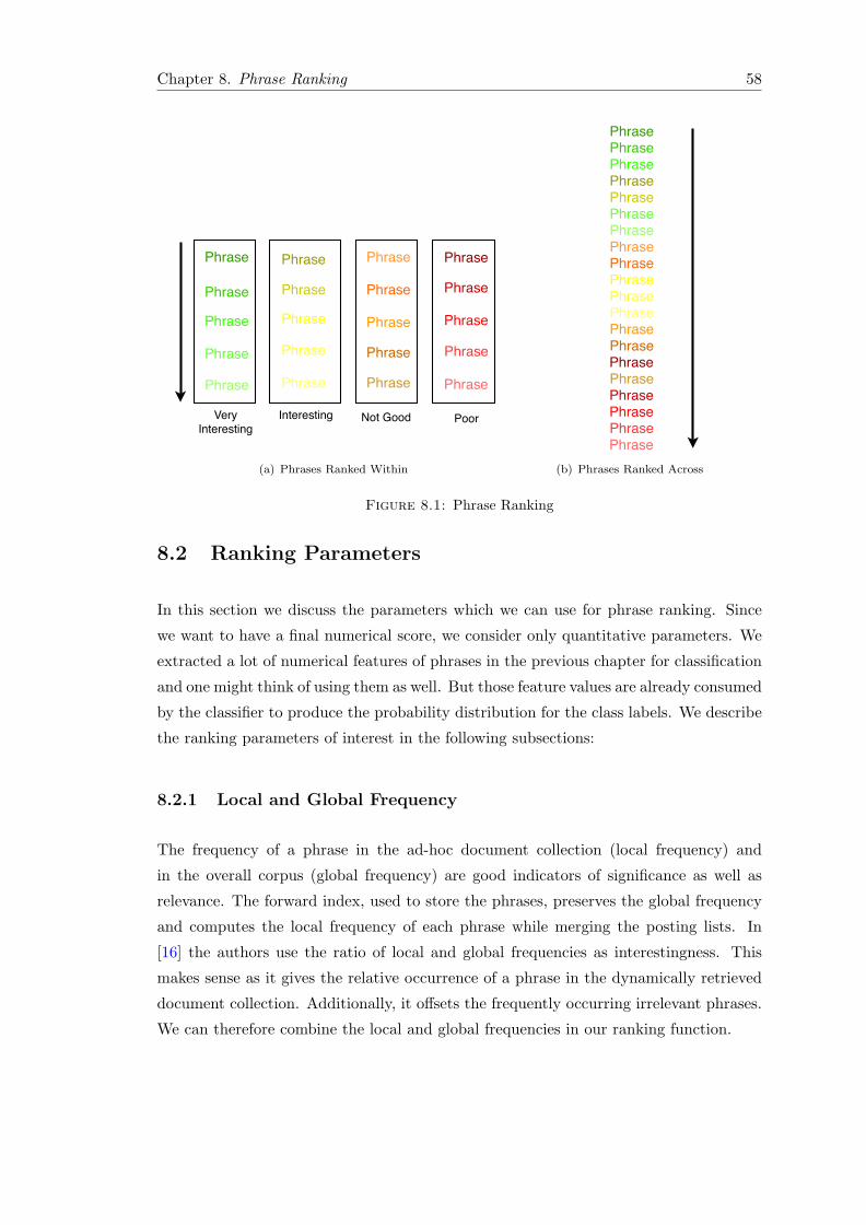
Chapter 8. Phrase Ranking 58
Phrase
Phrase
Phrase
Phrase
Phrase
Phrase
Phrase
Phrase
Phrase
Phrase
Phrase
Phrase
Phrase
Phrase
Phrase
Phrase
Phrase
Phrase
Phrase
Phrase
Very Interesting
Interesting Not Good Poor
(a) Phrases Ranked Within
PhrasePhrasePhrase
PhrasePhrase
PhrasePhrase
PhrasePhrasePhrase
PhrasePhrase
PhrasePhrase
PhrasePhrase
PhrasePhrasePhrasePhrase
(b) Phrases Ranked Across
Figure 8.1: Phrase Ranking
8.2 Ranking Parameters
In this section we discuss the parameters which we can use for phrase ranking. Since
we want to have a final numerical score, we consider only quantitative parameters. We
extracted a lot of numerical features of phrases in the previous chapter for classification
and one might think of using them as well. But those feature values are already consumed
by the classifier to produce the probability distribution for the class labels. We describe
the ranking parameters of interest in the following subsections:
8.2.1 Local and Global Frequency
The frequency of a phrase in the ad-hoc document collection (local frequency) and
in the overall corpus (global frequency) are good indicators of significance as well as
relevance. The forward index, used to store the phrases, preserves the global frequency
and computes the local frequency of each phrase while merging the posting lists. In
[16] the authors use the ratio of local and global frequencies as interestingness. This
makes sense as it gives the relative occurrence of a phrase in the dynamically retrieved
document collection. Additionally, it offsets the frequently occurring irrelevant phrases.
We can therefore combine the local and global frequencies in our ranking function.

Chapter 8. Phrase Ranking 59
8.2.2 Classification Distribution
The classification stage described in the previous chapter estimates the probability of
a phrase being in each of the class labels. Then it selects the label with maximum
probability as the predicted label. Apart from considering the predicted label, we can
also use the probability distributions of the class labels and combine them in an effective
manner. The combination can assign positive weights to the relevant labels (2 and 3)
and negative weights to the irrelevant ones (0 and 1).
8.2.3 Document Relevance
Apart from looking at phrase features, we can also look at the document containing
the phrase. The most obvious measure is the relevance of the document containing the
phrase. This tells us how much is the phrase relevant to the user query and consequently
how much is it likely to be interesting for the user. Search engines typically compute
document scores at query time to rank the documents. We can incorporate the same
scores in our ranking functions.
8.2.4 Size of document collection
Size of document collection is another dynamic measure which we can consider. This
gets especially important when comparing phrases from several queries in an OLAP
style analysis. The queries which fetch a small number of relevant documents could be
highly specific. Hence, a large set of phrases from them could be of interest to the user.
On the other hand, queries which fetch a large number of documents may need to prune
their phrase set more aggressively.
8.2.5 Document Rank
The parameters discussed above use only the dynamic properties of a phrase. We can
also use static measures like the static rank of the document containing the phrase.
This means that we rank the phrases retrieved from more important or authoritative
documents higher as compared to those from less authoritative documents. PageRank
is a widely used document rank and can be incorporated into the ranking function.

Chapter 8. Phrase Ranking 60
8.2.6 Global Statistics
The measurements so far use only the corpus local information. But we can also consider
global statistic from other popular information retrieval systems like web search engines.
Our document corpus being limited and restricted may not truly reflect the universal
appeal or interestingness of a phrase irrespective of the context or query. We can get
frequencies of a phrase and its individual terms and then use them to get a point-wise
mutual information (PMI) style measure. This can give an hint to the global surprise
factor associated with a particular phrase.
8.3 Ranking Functions
Currently, we use the probability distribution of the class labels for ranking and consider
the various ways to combine them. These include linear, logarithmic or exponential
combination of the parameters. However, to arrive at the right ranking function we
need to do relevance evaluation of our results. Below we discuss and describe some of
the ranking functions considered in our phrase mining system. Here p0, p1, p2 and p3
are the probabilities of labels 0,1,2 and 3 respectively:
Linear combination with positive weights: This scoring function simply assigns
the corresponding labels values as weights to the label probabilities. Label 0 gets a
weight of 0 and hence its corresponding probability does not contribute to the scoring
function. We illustrate the function as below:
Score = 3.p3 + 2.p2 + 1.p1 + 0.p0
Linear combination with positive and negative weights: This scoring function is
again a linear combination but allows both positive and negative weights. We consider
labels 3 and 2 as desirable and labels 1 and 0 as undesirable. Hence, probabilities of
label 3 and 2 have positive weights while the probabilities of label 1 and 0 have equally
negative weight. The function is as below:
Score = 2.p3 + 1.p2 − 1.p1 − 2.p0
Exponential combination: Instead of looking at each label individually, we can boost
the ranking score if relevant labels (2 and 3) have higher probabilities and punish if
irrelevant labels (0 and 1) have higher probabilities. This strategy pulls up the phrases
which have high probabilities for labels 2 and 3. Similarly, it pushes down phrases which
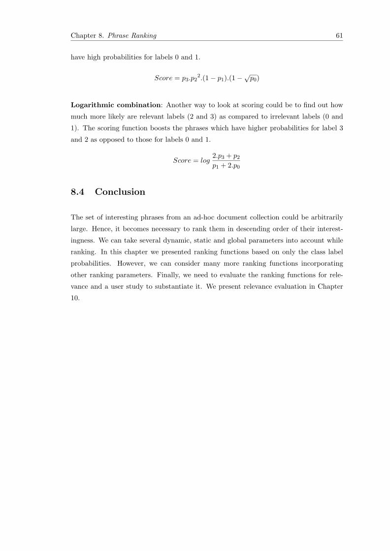
Chapter 8. Phrase Ranking 61
have high probabilities for labels 0 and 1.
Score = p3.p22.(1− p1).(1−√p0)
Logarithmic combination: Another way to look at scoring could be to find out how
much more likely are relevant labels (2 and 3) as compared to irrelevant labels (0 and
1). The scoring function boosts the phrases which have higher probabilities for label 3
and 2 as opposed to those for labels 0 and 1.
Score = log2.p3 + p2
p1 + 2.p0
8.4 Conclusion
The set of interesting phrases from an ad-hoc document collection could be arbitrarily
large. Hence, it becomes necessary to rank them in descending order of their interest-
ingness. We can take several dynamic, static and global parameters into account while
ranking. In this chapter we presented ranking functions based on only the class label
probabilities. However, we can consider many more ranking functions incorporating
other ranking parameters. Finally, we need to evaluate the ranking functions for rele-
vance and a user study to substantiate it. We present relevance evaluation in Chapter
10.

62

Chapter 9
Phrase Grouping
This chapter describes the grouping of phrases in the post-processing pipeline. The
ranking stage returns top-k results ranked by interestingness. However, the phrase
result set may still contain a lot of phrases on similar topics or domains. Such phrase
results may get boring for a user. At the same time, slightly lesser interesting phrases
from other domains could provide a better overview. Hence, for a holistic view we need
to diversify the top-k phrases. In this chapter we describe grouping of phrases based on
clustering and similarity. We discuss nouns and cosine similarities as two measures for
grouping.
9.1 Group by Clustering
The previous classification stage groups phrase into four classes. But we may need more
fine granular and dynamically derived groups. We can do this by clustering. A possible
way to do it is to use a subset of the phrase features for clustering. For instance, we
can use the term frequencies of words in the phrase to group phrases having same or
similarly frequent words. We can use popular clustering techniques like Expectation-
Maximization and k-Means. This machine learning based clustering can even precede
the ranking stage. Such a scenario will be akin to a two-stage machine learning. The first
stage creates clusters and the second stage labels phrases within each cluster. However,
the problem with machine learning based clustering is that it is hard to adjust the
clusters such that each cluster represents a separate topic. Hence, the features which we
use for clustering are crucial.
63

Chapter 9. Phrase Grouping 64
9.2 Similarity based Grouping
Apart from machine learning techniques, we can also group phrases based on similarity
between them. The objective is to form groups of most similar phrases. Since we need
grouping to be much more definitive, heuristics based features may not be suitable. We
take more suggestive artifacts such as nouns to group phrases. Once we have a similarity
measure, for a given phrase we find the phrases most similar to it. Next, we look up the
phrases which are most similar to this new phrase. We repeat this process recursively,
as long as we find phrases satisfying the lower threshold for similarity. This approach is
similar to connected components labeling.
Algorithm: Algorithm 9.1 takes a set of phrases and a similarity measure as inputs.
Line 1 initializes a set of groups to empty. Next we iterate over the set of phrases as long
as it contains ungrouped items (line 2). In each iteration, we pick a phrase, called the
root phrase, from the phrase set (line 3) and create a new group with the root phrase as
its element (line 4). Next, we populate the group with similar phrases from the phrase
set (line 5). We add the populated group to the set of groups (line 6). Finally, we return
the set of groups as the output (line 8).
Algorithm 9.2 populates the group with similar phrases. It takes a phrase set, a root
phrase, a similarity measure and a phrase group as inputs. Line 1 removes the root
phrase from the phrase set since it has been already added to the group. Next, we find
the phrase most similar, based on the similarity measure, to the root phrase (line 2).
If such a phrase exists then we add it to the group (line 3-4) and populate the group
recursively, considering the similar phrase as the root now (line 5). Else, we terminate
(line 6).
Algorithm 9.1: phraseGroupinginput : phrases, measureoutput: groups
Set groups←− {};1
while phrases 6= {} do2
Set root←− pickOne(phrases);3
Set group←− {phrase};4
populateGroup(phrases, root, measure, group);5
groups←− groups ∪ group;6
end7
return groups;8
Algorithm 9.3 finds the most similar phrase from the set of phrases for a given root
phrase. Line 1 initializes the similar phrase to NULL and line 2 sets the maximum
similarity to 0. Then we iterate over each phrase in the phrase set (line 3) and compute

Chapter 9. Phrase Grouping 65
Algorithm 9.2: populateGroupinput : phrases, root, measure, group
phrases←− phrases \ {root};1
Set similar ←− similarPhrase(root, phrases, measure);2
if similar ! = NULL then3
group←− group ∪ similar;4
populateGroup(phrases, similar, measure, group);5
end6
Algorithm 9.3: similarPhraseinput : root, phrases, measureoutput: similar
similar ←− NULL;1
maxSimilarity ←− 0;2
foreach Phrase p in phrases do3
Set currentSimilarity ←− measure(root, p);4
if currentSimilarity > maxSimilarity then5
Set similar ←− p;6
Set maxSimilarity ←− currentSimilarity;7
end8
end9
return similar;10
its similarity with the root phrase (line 4). If the similarity is greater than the maximum
similarity seen so far then we set the similar phrase to the current phrase in the iteration
and maximum similarity to the current similarity (line 5-7). Finally, we return the most
similar phrase found in this fashion (line 10).
Analysis: In terms of complexity, essentially the algorithm has two nested loops of
iteration over the set of phrases. First reaction would be think the time complexity
to be quadratic with the number of phrases. But note that we eliminate the grouped
phrases from the phrase set. Hence, the phrase set keeps on shrinking depending on the
size of the groups. In the worst case, each group contains a single element (i.e. no groups
formed) and the time complexity would be O(n2), where n is the number of phrases in
the input set. Whereas in the best case when we group all phrases into a single group,
the time complexity would be O(n), where n is the number of phrases in the input set.
This is because we need only a single parse over the input set of phrases. However, both
these extremes are unexpected. Below we analyze the time complexity of our grouping
algorithm assuming an average group size p:
Consider a phrase set S with n phrases:
|S| = n

Chapter 9. Phrase Grouping 66
Assume the average size of the groups to be p. Now consider the number of iterations
over the phrase set. For the first parse, on the first phrase, we check all remaining
phrases for similarity, i.e:
#Iteration1 = n− 1
For the second parse only the phrases still left ungrouped are iterated, i.e.:
#Iteration2 = n− 1− p
For groups of average size p, n/p passes would be required. Summing up, the total
number of iterations is:
#Iterations = (n− 1) + (n− 1− p) + (n− 1− 2p) + (n− 1− 3p) + ...+ (n− 1− (n
p− 1)p)
=n
p(n− 1)− [p+ 2p+ 3p+ ...+ (
n
p− 1)p]
=n2
p− n
p− p[1 + 2 + 3 + ...+ (
n
p− 1)]
=n2
p− n
p− p[ n
2p(n
p− 1)]
#Iterations =n2
2p− n
p+n
2
The time complexity of the above algorithm is O(n2
p −np +n). For p of the order of O(n)
(e.g. p = n/10), the complexity becomes linear i.e. O(n).
9.2.1 Noun Similarity
The previous description of grouping algorithm still leaves the similarity measure as an
abstraction. By inspecting the phrases, we realize that nouns are the most likely indi-
cators of the domain or the topic of the phrases. In this similarity measure we compute
the number of common nouns between two phrases. We consider the phrases having the
maximum number of nouns in common as similar. We expect the interesting phrases
to contain the nouns pertinent only to their domain. With this we can treat nouns as
the keywords for the phrases and use them as grouping parameters. As an example,
query “bill gates” produces all phrases about Microsoft like “Microsoft’s founder bill
gates” and “A microsoft sponsored conference” in a single group. We express the noun
similarity between two phrases as follows:
Simnoun(phrase1, phrase2) = |nouns(phrase1) ∩ nouns(phrase2)|

Chapter 9. Phrase Grouping 67
9.2.2 Cosine Similarity
Instead of just using one attribute, we can use a list of attributes for comparing sim-
ilarity. The attributes can be modeled as a feature vector as explained in Chapter 7.
Consequently, we can compute cosine similarity between the feature vectors as defined
below:
Simcosine(phrase1, phrase2) =−−−−−−−−−−−−−−−−−→featureVector(phrase1) ·
−−−−−−−−−−−−−−−−−→featureVector(phrase2)
|featureVector(phrase1)| × |featureVector(phrase2)|
9.3 Conclusion
Grouping is necessary for better user accessibility and to diversify the phrases across a
variety of topics. We can create groups dynamically using clustering. But this requires
precise feature set. We can also do grouping using noun similarity between phrases. For
this, however, we need a fair number of nouns to be present in the phrases. However,
we have the risk of the groups having too less (over-grouping) or too many (under-
grouping) phrases. The cosine similarity can be used as another measure for similarity.
Finally, getting the right granularity of groups is a challenge and it needs a user study
for evaluation.

68

Chapter 10
Experimental Evaluation and
Results
This chapter discusses the experimental evaluation of our phrase mining system. We
proposed several strategies for processing in the post-processing pipeline in the previous
chapters. We now need to analyze the processing cost versus the quality benefits of
these strategies to be able to justify their use. In this chapter we first describe the
experimental setup, then we present brief results and finally we discuss the evaluation
results.
10.1 Experimental Setup
10.1.1 System Configuration
We developed the phrase mining system and did the experiments on a MacBook Pro
machine running Max OS X Version 10.5.8 on 2.53 GHz Intel Core 2 Duo processor, 4
GB 1067 MHz DDR3 memory and 320 GB of disk storage. We did the development
in Java 1.6.0. We averaged all experimental results over at least 3 trials. We used the
Phrase Forward index, as proposed by Srikanta et al. [16], to store the phrases. We used
the following external software packages: Stanford Parts-Of-Speech Tagger [8] version
1.6, Weka Data Mining Software for Java [11] version 3-6-1 and WordNet [13] version 3.0.
Additionally, we use the stop words lists [9] maintained by the Linguistics Department
at University of Glasgow.
69

Chapter 10. Experimental Results and Evaluation 70
10.1.2 Data set
We used the recently released news archives from New York Times [5] as data set in our
experiments. It contains over 1.8 million annotated news articles written and published
by the New York Times between January, 1987 and June, 2007. The GZIP compressed
data file of the corpus is 2.4 GB in size. The phrase forward index built on this corpus
is 11.9 GB in size. Later we tag the phrase forward index to contain the POS and the
Named Entity tags along with the phrases. The tagged phrase forward index is 18 GB
in size. We discuss the tagging of phrase forward index in more detail in Chapter 11.
10.1.3 Experiments
There are three stages in the experiments on phrase mining system. First, we manually
label representative phrases. Next, we use the labeled data to train the classifier. Finally,
we post-process the candidate phrases, obtained from testing queries, through the post-
processing pipeline. We evaluate the final set of phrases for the following metrics:
1. Overall precision of relevant phrases.
2. The recall of relevant phrases through post-processing pipeline.
3. Precision and recall through the processing stages in the pipeline.
4. Time latency of the stages in the processing pipeline.
5. Filtering effectiveness i.e. number of phrases filtered through each stage.
6. Cross validation to evaluate the classifier.
7. Normalized discounted cumulative gain (NDCG) to evaluate the ranking function.
Queries: We select 5 queries (training queries) and produce over 200 phrases from each
of them (1100 phrases in total). Table 10.1(a) lists the training queries. To reduce the
personal bias, two computer science masters students manually label these 1100 phrases.
We select 6 more representative queries (testing queries) which are different from the
training queries. Table 10.1(b) lists the testing queries. We need to additionally label
the candidate phrases from the testing queries for the evaluations.

Chapter 10. Experimental Results and Evaluation 71
(a) Training Queries
Jennifer LopezOsama Bin LadenEminemWorld Trade CenterAmerican Airlines
(b) Testing Queries
Ronald ReaganBill GatesIraq WarBrad PittAfghanistanGoogle Founder
Table 10.1: Training and testing queries
10.2 Results
10.2.1 Ranked Results
We rank the phrases from each of the training queries using the following linear ranking
function with both positive and negative weights:
RankScore = 2.p3 + 1.p2 − 1.p1 − 2.p0
The above ranking function was observed to be performing good in our experiments.
Here, p3, p2, p1 and p0 are the probabilities of class label 3, 2, 1 and 0 resectively. Table
10.2 shows the top-10 phrases that we obtain for query “Ronald Reagan” and rank by
the above ranking function.
Rank Phrase1 Lead former president ronald reagan died2 Comparing the styles and policies3 The reagan biography4 Governor reagan his rise to power5 Loving brother of mary anne stalter6 The real reagan according to deaver7 84. died february 18. of white river junction8 I now begin the journey9 The statements coming from oliver10 Former president’s funeral and a related
Table 10.2: Top-10 phrases for “Ronald Reagan”
We can observe that most of the result phrases are unique and do not contain duplicate
information. Additionally, the phrases in the result set are complete i.e. they are more or
less not broken and make some sense. More importantly, many of them contain elements
of interest like Reagan’s death, his styles and policies, his biography, his rise to power,
his funeral etc. However, we still see many phrases from the same topic. For instance,
three to four phrases in the above list are concerning to his demise.
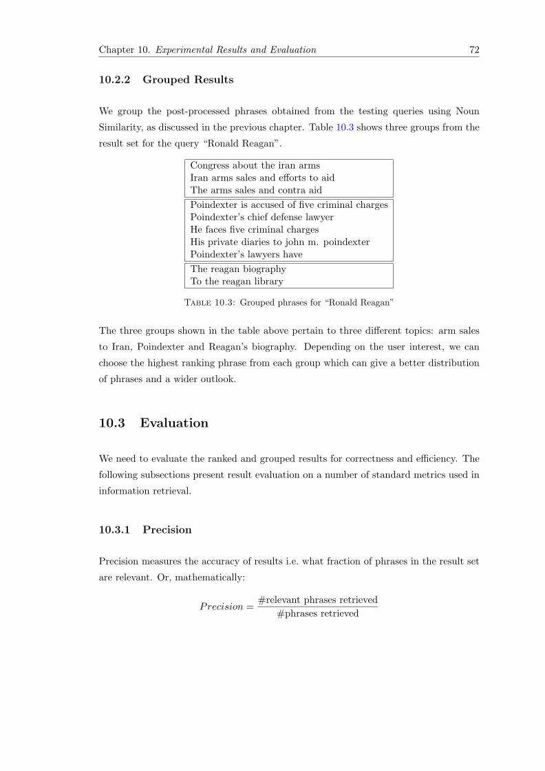
Chapter 10. Experimental Results and Evaluation 72
10.2.2 Grouped Results
We group the post-processed phrases obtained from the testing queries using Noun
Similarity, as discussed in the previous chapter. Table 10.3 shows three groups from the
result set for the query “Ronald Reagan”.
Congress about the iran armsIran arms sales and efforts to aidThe arms sales and contra aidPoindexter is accused of five criminal chargesPoindexter’s chief defense lawyerHe faces five criminal chargesHis private diaries to john m. poindexterPoindexter’s lawyers haveThe reagan biographyTo the reagan library
Table 10.3: Grouped phrases for “Ronald Reagan”
The three groups shown in the table above pertain to three different topics: arm sales
to Iran, Poindexter and Reagan’s biography. Depending on the user interest, we can
choose the highest ranking phrase from each group which can give a better distribution
of phrases and a wider outlook.
10.3 Evaluation
We need to evaluate the ranked and grouped results for correctness and efficiency. The
following subsections present result evaluation on a number of standard metrics used in
information retrieval.
10.3.1 Precision
Precision measures the accuracy of results i.e. what fraction of phrases in the result set
are relevant. Or, mathematically:
Precision =#relevant phrases retrieved
#phrases retrieved

Chapter 10. Experimental Results and Evaluation 73
In our setting we label the set of candidate phrases for the testing queries. We define
relevance as follows:
Relevance =
relevant, if label = 3 or label = 2
irrelevant, if label = 1 or label = 0
To measure precision, we scan the final result set from post-processing to find out how
many relevant phrases are retained. However, since post-processing merges the phrases,
full string comparison alone may not work. We also need to look at phrase substrings.
Figure 10.1 shows the precision variation for the six test queries listed in Table 10.1(b).
0
0.2
0.4
0.6
0.8
Ronald
Reagan
Bill
Gate
s
Iraq W
ar
Bra
d P
itt
Afg
hanis
tan
Founder
0.71
0.658
0.6250.605
0.763
0.73
Pre
cis
ion
Figure 10.1: Precision variation by query
We can observe precision values between 0.6 and 0.8. We can attribute lower precision
to either of the following two reasons:
1. We still have lots of irrelevant phrases in the result set. This implies that we still
have room for more aggressive filtering.
2. We could be filtering out many of the relevant phrases.
We describe the recall measure in the next subsection to understand this better.

Chapter 10. Experimental Results and Evaluation 74
10.3.2 Recall
Recall measures the fraction of the relevant phrases present in the result set. In phrase
mining it is difficult to estimate the total number of relevant phrases in the whole index.
To simplify things, we assume that the initial set of candidate phrases obtained from the
Forward Index contains all the relevant phrases. In other words we measure the recall
of relevant phrases through the post-processing pipeline only. We can express the recall
of relevant phrases as:
Recall =#relevant phrases retrieved
#relevant phrases
Again, we use the labeled set of phrases for the test queries and compare how many of
the relevant phrases persist in the output set of phrases. Figure 10.2 shows the recall of
relevant phrases for six different testing queries.
0.6
0.7
0.8
0.9
1
Ronald
Reagan
Bill
Gate
s
Iraq W
ar
Bra
d P
itt
Afg
hanis
tan
Founder
0.88
0.903
0.845
0.757
0.851
0.914
Re
ca
ll
Figure 10.2: Recall variation by query
We can see that the recall values lie between 0.75 and around 0.9. Apart from the query
“Brad Pitt” all other queries have recall better than 0.8. The recall value for the query
“Brad Pitt” is unusually low and this could be because of the lesser range of interesting
things about him in the corpus.

Chapter 10. Experimental Results and Evaluation 75
10.3.3 Precision/Recall Variation in Post-Processing
So far we have evaluated precision and recall across the post-processing pipeline. But
we also need to evaluate them within the pipeline to see which stages impact the most.
Figure 10.3 shows the variation of the precision values across different stages in the
pipeline.
0
0.2
0.4
0.6
0.8
Cust
om
Edito
r
Sto
pW
ord
sMer
ge
Syn
onym
Mer
ge
Pre
fixS
uffix
Filt
er
PO
SFilt
er
Fuss
ySuffix
Filt
er
Sim
ple
Heu
rist
ics
Cla
ssifi
catio
nFilt
er
MLC
lust
er
Precision Variation (by query)
Ronald Reagan Bill Gates Iraq WarBrad Pitt Afghanistan Google FounderP
rec
isio
n
Figure 10.3: Precision variation in the post-processing pipeline
As we can see, initially the precision value is between 0.4 and 0.6 and gradually it
gets better as phrases are processed through the pipeline and finally the precision value
ranges between 0.6 and 0.8. Similarly, Figure 10.4 shows the variation of the recall
values through the post-processing pipeline.
Here, we can see that the recall values start from 1 and diminishing through the pipeline.
The final recall values lie in the range of 0.75 to 0.9.
10.3.4 Filtering Effectiveness
Similar to measuring precision and recall across different stages in the pipeline, we would
also like to measure the number of phrases filtered (called the filtering effectiveness) in
each stage in the pipeline. We measure filtering effectiveness as the reduction in the
cardinality of the candidate set across a stage.
Filtering Effectiveness = #input phrases−#output phrases

Chapter 10. Experimental Results and Evaluation 76
0
0.25
0.5
0.75
1
Cust
om
Edito
r
Sto
pW
ord
sMer
ge
Syn
onym
Mer
ge
Pre
fixS
uffix
Filt
er
PO
SFilt
er
Fuss
ySuffix
Filt
er
Sim
ple
Heu
rist
ics
Cla
ssifi
catio
nFilt
er
MLC
lust
er
Recall Variation (by query)
Ronald Reagan Bill Gates Iraq WarBrad Pitt Afghanistan Google Founder
Re
ca
ll
Figure 10.4: Recall variation in the post-processing pipeline
0
75
150
225
300
Custo
mFilt
er
ExactM
erg
e
Custo
mE
ditor
Sto
pW
ord
sM
erg
e
Syn
onym
Merg
e
Pre
fixS
uff
ixFilt
er
PO
SFilt
er
FussyS
uff
ixFilt
er
Sim
ple
Heuri
stics
Cla
ssific
ationFilt
er
MLC
luste
r
0
23.833
00.167
39.333
18.667
09.333
0
259.333
2.833
Nu
mb
er
(Avg
) o
f fi
lte
red
ph
rase
s
Figure 10.5: Filtering effectiveness of stages in the post-processing pipeline

Chapter 10. Experimental Results and Evaluation 77
0
125
250
375
500
100 200 300 400 500
Filtering Vs Number of Input Phrases
Ronald Reagan Bill Gates Iraq WarBrad Pitt Afghanistan Google Founder
Nu
mb
er
of
Filte
red
Ph
rase
s
Figure 10.6: Filter scalability with candidate set size
Figure 10.5 shows the decrease in the size of the candidate set of phrases after each stage.
Initial set of phrases contain 500 phrases and we have averaged the numbers shown over
the 6 testing queries.
As shown in the figure, exact merge which includes prefix, suffix and prefix-suffix merge,
is the most effective stage in the post-processing pipeline. The merge operation depends
on the number of input phrases. Hence, a large candidate set may have more phrases
pruned out. Figure 10.6 shows the variation in filtering effectiveness by varying the size
of the initial candidate set from 100 to 500. Not surprisingly, filtering scales linearly with
the size of the initial phrase set. However, a large number of input phrases can be merged
and therefore add more meaning to the broken or incomplete phrases. Consequently, we
observe the quality of results to be higher with a larger number of input phrases. Hence,
size of the candidate set of phrases is an important consideration.
10.3.5 Processing Latencies
In the last subsection we discussed how larger phrase sets could produce better quality
results. This, however, comes with the price of processing latencies. The post-processing
of phrases is expensive and at query time. The system must therefore have an acceptable
response time. We need to analyze the time taken by each stage in the post-processing
pipeline and then see how much we gain at the price of this latency. We measure latencies

Chapter 10. Experimental Results and Evaluation 78
by noting the time difference between the start and the end of processing in a stage.
TimeLatency = End Time− Start Time
Figure 10.7 shows the time latencies (in secs) for different stages in the post-processing
pipeline. Again, we average the values over the 6 test queries.
0
3.75
7.5
11.25
15
Custo
mFilt
er
ExactM
erg
e
Custo
mE
ditor
Sto
pW
ord
sM
erg
e
Syn
onym
Merg
e
Pre
fixS
uff
ixFilt
er
PO
SFilt
er
FussyS
uff
ixFilt
er
Sim
ple
Heuri
stics
Cla
ssific
ationFilt
er
MLC
luste
r
0.00300.583
0.002
3.649
0.001
13.401
0.2520.0090.324
0.009
Exe
cu
tio
n T
ime
(se
c)
Figure 10.7: Post-processing stage-wise latencies
As we see from the figure, synonym merge has the maximum time latency. This is
because it has to look up the synsets for each word in the WordNet database. Another
bottleneck is the parts-of-speech filter (POS Filter). The POS filter has to identify the
parts-of-speech of the terms in the phrase and hence the delay.
10.3.6 Cross Validation
An n-fold cross validation is the standard technique to evaluate the accuracy of the
classifier. The idea is that the training set is divided into n sets and one set is chosen for
testing while the remaining sets are used to train the classifier. This way the percentage
of correctly classified instances are measured and it is averaged over all sets of testing
phrases.
In our experiments we perform 4-fold cross validation to measure the accuracy of the
classifier. We have used multilayer perceptron for classification, but we compare the
accuracy of several classifiers on our training data set. Figure 10.8 shows the percentage
accuracy i.e. the percentage of correctly classified items, for several classifiers.
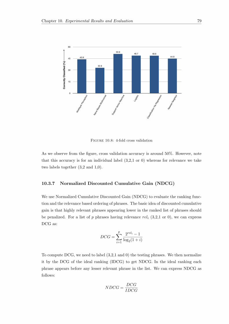
Chapter 10. Experimental Results and Evaluation 79
0
15
30
45
60
Multi
laye
r P
erce
ptron
Nai
ve B
ayes
Multi
nom
ial
Support
Vec
tor M
achin
e
Logis
tic
Cla
ssifi
catio
n V
ia R
egre
ssio
n
Nea
rest
Nei
ghbor
44.8
48.648.750.9
32.9
43.9
Co
rre
ctl
y C
lassif
ied
(%
)
Figure 10.8: 4-fold cross validation
As we observe from the figure, cross validation accuracy is around 50%. However, note
that this accuracy is for an individual label (3,2,1 or 0) whereas for relevance we take
two labels together (3,2 and 1,0).
10.3.7 Normalized Discounted Cumulative Gain (NDCG)
We use Normalized Cumulative Discounted Gain (NDCG) to evaluate the ranking func-
tion and the relevance based ordering of phrases. The basic idea of discounted cumulative
gain is that highly relevant phrases appearing lower in the ranked list of phrases should
be penalized. For a list of p phrases having relevance reli (3,2,1 or 0), we can express
DCG as:
DCG =p∑i=1
2reli − 1log2(1 + i)
To compute DCG, we need to label (3,2,1 and 0) the testing phrases. We then normalize
it by the DCG of the ideal ranking (IDCG) to get NDCG. In the ideal ranking each
phrase appears before any lesser relevant phrase in the list. We can express NDCG as
follows:
NDCG =DCG
IDCG
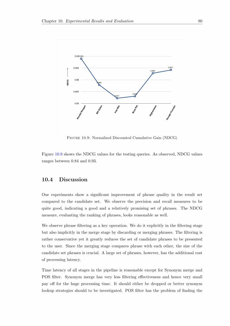
Chapter 10. Experimental Results and Evaluation 80
0.83
0.855
0.88
0.905
0.93
Ronald
Reagan
Bill
Gate
s
Iraq W
ar
Bra
d P
itt
Afg
hanis
tan
Founder
0.925
0.869
0.8410.845
0.894
0.901N
DC
G
Figure 10.9: Normalized Discounted Cumulative Gain (NDCG)
Figure 10.9 shows the NDCG values for the testing queries. As observed, NDCG values
ranges between 0.84 and 0.93.
10.4 Discussion
Our experiments show a significant improvement of phrase quality in the result set
compared to the candidate set. We observe the precision and recall measures to be
quite good, indicating a good and a relatively promising set of phrases. The NDCG
measure, evaluating the ranking of phrases, looks reasonable as well.
We observe phrase filtering as a key operation. We do it explicitly in the filtering stage
but also implicitly in the merge stage by discarding or merging phrases. The filtering is
rather conservative yet it greatly reduces the set of candidate phrases to be presented
to the user. Since the merging stage compares phrase with each other, the size of the
candidate set phrases is crucial. A large set of phrases, however, has the additional cost
of processing latency.
Time latency of all stages in the pipeline is reasonable except for Synonym merge and
POS filter. Synonym merge has very less filtering effectiveness and hence very small
pay off for the huge processing time. It should either be dropped or better synonym
lookup strategies should to be investigated. POS filter has the problem of finding the

Chapter 10. Experimental Results and Evaluation 81
parts-of-speech at query time. This can be avoided by doing parts-of-speech tagging at
index level itself. This idea and implementation is elaborated in more detail in Chapter
11.
The final results presented to the user can be organized in many ways. We produce the
best effort result set which is likely to be interesting. However, the phrases presented
to a user may still be too broad. Thus, we may need user personalization to cater to
specific user interests.
10.5 Conclusion
Experiments are a crucial part of any scientific study. In our experiments we use news
archive data from New York Times. However, one can use data corpus from other
domains like blogs, emails and other user generated content to run similar experiments
and draw the parallels. We used several measures from information retrieval literature
to evaluate the system. The experimental results obtained in this thesis underscore the
potential of phrase mining and encourage the possibility of future work.

82

Chapter 11
Further Optimizations
This chapter describes further optimization in our phrase mining system. The exper-
imental evaluations in the previous chapter show some stages in the post-processing
pipeline to be computationally expensive. These slow straggler stages must be opti-
mized. To avoid query time latencies, we need to push post-processing down the pro-
cessing pipeline and indexing levels as much as possible. Additionally, the size of the
phrase index is a concern. We can understand the merging and filtering patterns over
time and embed the intelligence into the system to prune the phrase index. We discuss
parts-of-speech tagging, named entity tagging and phrase index pruning in this chapter.
11.1 Forward Index Translation
A forward index is used to store the phrases as described in Chapter 2. By default
the forward index stores the global frequencies of phrases and computes local frequency
dynamically at query time. However, we can store other things such as parts-of-speech
along with the global frequency and save significant computation time during the query
processing. This could even increase the accuracy because the phrase properties ex-
tracted at the indexing time have full view of the corpus. We must pack the properties
extracted in such a manner into the forward index. We call this operation as forward
index translation i.e. translating forward index to stuff additional information.
Two such properties are the parts-of-speech of the terms in a phrase and the named
entities contained in a phrase. We have used these two features in the post-processing
and they have considerable latency when extracted at query time. Additionally, the
parts-of-speech and the named entities being natural language artifacts, they need at
least full sentences if not full documents to be effectively accurate. Below we describe
their extraction and the corresponding forward index translation.
83

Chapter 11. Further Optimizations 84
Figure 11.1 depicts the process of forward index translation. We are given a text cor-
pus and a forward index created previously (denoted by hashed line). We now want
to add to it the parts-of-speech and the named entities information for each phrase.
We parse the documents corresponding to each of the document identifiers (did) in the
text corpus. We tokenize each of the documents using a tokenizer. We then send the
the tokenized document to a parts-of-speech tagger and a named entity recognizer to
extract the parts-of-speech and the named entities respectively. The index translator
then queries the phrase index by the document identifier (did) and gets the correspond-
ing phrase list. It adds the parts-of-speech and the named entities information to each
phrase in the phrase list. Finally, we store the tagged phrases into a translated forward
index.
TextCorpus
ForwardIndex
TokenizeParts-Of-Speech
Tagger
Named Entity Recognizer
TranslateTranslatedForward
Index
diddocument
POS Tags
Named Entities
did
< phrase >
Figure 11.1: Forward Index Translation
In the above design we tokenize and tag the whole document. We need to locate each
phrase back in the corpus to add the parts-of-speech and the named entities information
to it. It can be very hard to trace back the phrases in the corpus since they are arbitrary
subset of words in a document . Fortunately, the forward index stores posting lists for
each document and hence the document can be easily traced. Within a document,
however, we still need to locate the phrase. We do this by running a sliding window over
the content of the document.
Implementation wise, we can pack the parts-of-speech tag and the named entity tag into
the posting lists in two ways. Since the forward index already stores the phrases as a
list of integer term identifiers, we can add the integer encoded tags as extra terms into
the phrase as shown in Figure 11.2(a). Second way to pack the tags is to put them
next to the phrase separately without touching the phrase as shown in Figure 11.2(b).
The second way is cleaner and provides a concrete segregation between the phrase and

Chapter 11. Further Optimizations 85
the tags. This makes the use of tags optional and we can safely skip them, without
modifying phrase processing, in case they are not required.
Phrase POS NamedEntities
(a) Implicit Phrase Layout
Phrase POS NamedEntities
(b) Explicit Phrase Layout
Figure 11.2: Phrase Layout options
Next, we describe the encoding of the parts-of-speech and the named entity tags into
integer representations. The parts-of-speech tag contains the part-of-speech for each
word in the phrase. We use 32 major tags from the Penn Treebank tag-set [6]. Hence,
we can encode each POS with 5 bits and pack up to 6 terms in one 4-byte integer as
shown in Figure 11.3.
0 5 10 15 20 25 30
POS 1 POS 2 POS 3 POS 4 POS 5 POS 632
Figure 11.3: POS tag encoding
The named entity tag contains the start index, the end index and the type of the named
entity in a phrase. For phrases having up to 8 terms, 3 bits are sufficient for start and
end indices. The named entities can be of type person, location or organization. We
need one bit for each because the same terms can be multiple named entities in different
parts of the document. Thus each named entity takes 9 bits and for each phrase we can
pack 3 named entities in one 4-byte integer as shown in Figure 11.4.
11.2 Forward Index Pruning
The previous section described how by pushing things down to indexing level we can
save processing time while querying. Another class of optimization is to reduce the set
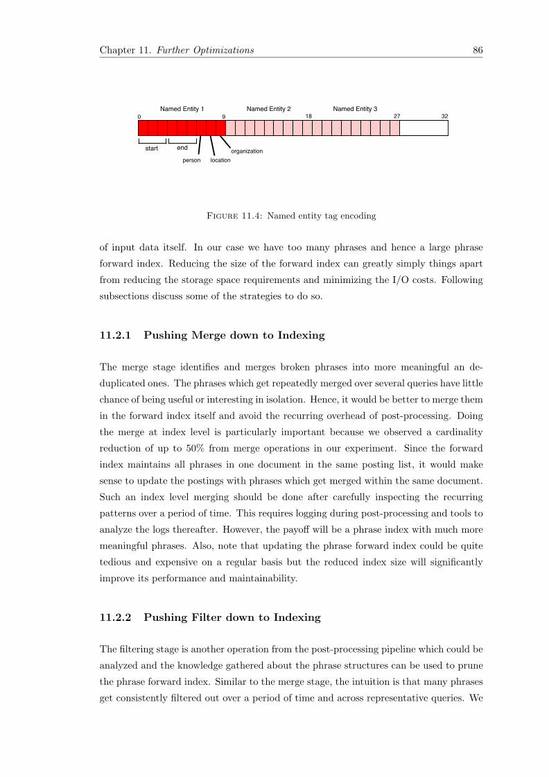
Chapter 11. Further Optimizations 86
start end
person locationorganization
0 9 18 27 32Named Entity 1 Named Entity 2 Named Entity 3
Figure 11.4: Named entity tag encoding
of input data itself. In our case we have too many phrases and hence a large phrase
forward index. Reducing the size of the forward index can greatly simply things apart
from reducing the storage space requirements and minimizing the I/O costs. Following
subsections discuss some of the strategies to do so.
11.2.1 Pushing Merge down to Indexing
The merge stage identifies and merges broken phrases into more meaningful an de-
duplicated ones. The phrases which get repeatedly merged over several queries have little
chance of being useful or interesting in isolation. Hence, it would be better to merge them
in the forward index itself and avoid the recurring overhead of post-processing. Doing
the merge at index level is particularly important because we observed a cardinality
reduction of up to 50% from merge operations in our experiment. Since the forward
index maintains all phrases in one document in the same posting list, it would make
sense to update the postings with phrases which get merged within the same document.
Such an index level merging should be done after carefully inspecting the recurring
patterns over a period of time. This requires logging during post-processing and tools to
analyze the logs thereafter. However, the payoff will be a phrase index with much more
meaningful phrases. Also, note that updating the phrase forward index could be quite
tedious and expensive on a regular basis but the reduced index size will significantly
improve its performance and maintainability.
11.2.2 Pushing Filter down to Indexing
The filtering stage is another operation from the post-processing pipeline which could be
analyzed and the knowledge gathered about the phrase structures can be used to prune
the phrase forward index. Similar to the merge stage, the intuition is that many phrases
get consistently filtered out over a period of time and across representative queries. We
Chapter 11. Further Optimizations 87
can infer such phrases as junk or spam and hence discarded them permanently from the
forward index.
11.3 Conclusion
We can optimize several stages in the post-processing pipeline or push them down to the
indexing level. The forward index translation with tags stored along with their phrases
can avoid doing the parts-of-speech and the named entity tagging at query time. We
can push the merging and filtering stages down to indexing level in order to prune the
forward index to a much smaller size. The ideal scenario would be to apply the merge,
filter and classify stages at the forward index building time. We should need only the
ranking and the grouping stages at query time.

88

Chapter 12
Conclusion and Future Work
In today’s world there is a ubiquity of textual data. Ideally, the data should be struc-
tured but majority of the data is unstructured. Text analytics on such data is a highly
specialized task, but spans broad reaching topics having applications in life sciences,
financial services, legal, retail, government, media, and entertainment, to name a few.
Phrase mining, as a special case of text analytics, produces interesting phrases to un-
derstand and analyze the potentially valuable data. However, several aspects of phrase
mining need to be considered.
Understanding interestingness: A major challenge in mining phrases of interest is
to understand the interest itself. Usually we ask the end users to distinguish between
interesting and uninteresting phrases. But the set of candidate phrases, for a given user
query, is too big and noisy. This gave the need to statically define the interestingness
of phrases. Prior works proposed a single statistics based definition of interestingness.
However, this is not sufficient to characterize and capture the potentially interesting
phrases. In this work we tried to define and generalize some static properties of interest-
ingness. Consequently, we suggested an elaborate post-processing of phrases to surface
the ones having these properties.
Interestingness, however, can be a far more reaching property. Apart from structural
sanctity, interestingness can also mean a very wide range of other things in a general
sense. The most common being the presence of factual content in the phrases. We can
extract these factual mappings from ontology databases. Temporal events are another
set of things which could be of interest but are more difficult to extract. The author
sentiment could also be of great interest especially when the tone is strongly opinionated.
The cultural connotation connect better to some users and hence could be of interest.
Finally, result personalization based on end user preferences could be a great boost.
89

Chapter 12. Conclusion and Future Work 90
The same set of “interesting” phrases can be hot interesting for one user and lukewarm
interesting for another. We need to discern the interestingness in the two cases.
Our System: This work attempts to put an elaborate and in depth approach to phrase
mining. We presented an end to end phrase mining system integrable with any docu-
ment style information retrieval system. We started by analyzing different aspects of
interestingness and the challenges to it. Our aim was to evaluate the phrases on each of
these aspects of interestingness and extract them in the form of features. The idea was
to generate a feature set which characterizes the phrases to the greatest possible extent.
The features arranged in the form of the feature vectors were then used to predict the
interestingness of the phrases using a supervised machine learning technique. Subse-
quently, we ranked and grouped the predicted phrases for a listed view and a diversified
result set respectively. We evaluated the phrase mining system using a range of experi-
ments and analyzed the results. The results from the experiments are encouraging and
strengthen the potential of phrase mining on an ad-hoc document collection. We can
do many optimizations throughout the post-processing pipeline and we have discussed
some of them in detail. Additionally, we proposed methods to prune the size of the
phrase forward index.
The major stumbling block faced in this work was the concrete and precise definition of
interestingness. Other challenges include choosing the threshold confidence factors for
merging and filtering operations, defining and extracting a truly characterizing feature
set, labeling the training data, choosing the appropriate classifier, arriving at the most
suitable ranking function and choosing the right similarity measure for creating groups
of phrases.
Managing the expectations: An important thing about phrase mining is to set
the expectations properly. Users might argue the presence of some highly interesting
phrases in the corpus but these phrases may not be frequent enough to be present in the
phrase forward index. The concerned persons should understand the design decisions and
constraints of the phrase mining system to be able to make better use of the technology.
Coming of an age: Search engines need to incorporate more phrase mining style text
analytics. Though phrase mining resembles information retrieval systems like web search
engines more than business intelligence systems, it strikes the middle ground between
the two. A couple of decades ago, web search was considered to be experts’, called
“professional searchers”, prerogative. Advances in search technology and the advent of
better user interfaces have resulted the web search engines to come of an age. In similar
spirit, we expect the horizons of phrase mining to go well beyond just trained analytics
and hope that an amalgam of search engine and phrase mining will become a natural
choice in the future.
Chapter 12. Conclusion and Future Work 91
12.1 Future Work
Alternate Techniques: Several strategies and methods employed in the various stages
of the post-processing pipeline use standard textbook techniques from the domains of
algorithms, information retrieval and natural language processing. They have a con-
siderable scope for improvement. The merging and grouping stages, for instance, make
use of similarity measures which have been extensively researched over the past several
years. The applicable ideas from many such research and development could be studied
and applied in our setting. Similarly, more ideas for classification and ranking could be
inspired from IR literature whereas parts-of-speech and named entity tagging from NLP
literature.
Post-processing Pipeline Pruning: As discussed in Chapter 11, we can push many
stages in the post-processing pipeline down to the indexing level. This is on similar
lines as query optimization in database community where operators are pushed down
the query processing as much as possible. The advantage of doing this in phrase mining,
same as in databases, is to have lesser data and lesser computations as we move through
the post-processing. Additionally, in our case the entire set of phrases is not really
mandatory to maintain. It was created in brute force fashion by considering only a
lower threshold frequency to decide whether or not to keep a phrase. While this suits
well at index creation time, we can use the phrase related knowledge gathered from the
post-processing over a period of time and apply it to the phrase index. Hence, we can
enrich the quality of phrases inherently and transform the phrase index into an index of
interesting phrases. The goal should be to have as few stages in the post-processing as
possible.
Text Granularity: Currently there are two extremes of text mining: the document
granular search engines and the word granular keyword analysis tools. While in this
work we present a case for interesting phrases, several times single word keywords are
interesting as well. Conversely in many other scenarios phrases seem to be too short
to be expressive and full sentences, summary snippets or even the whole document is
needed to make it interesting. Thus, interestingness should only be based on the static
properties and the user taste and not on the length of the text. To this end a flexible
granularity approach for text mining could be taken which considers words, phrases,
sentences and documents for interestingness. This could be a hybrid of existing systems
for each granularity level or it could be a completely new system redefining the text
mining altogether.
Semantic Sense: Our phrase mining system proposed in this work relies more or less
on three essentials: 1) statistics (frequencies and other heuristics) 2) linguistics (parts

Chapter 12. Conclusion and Future Work 92
of speech and sentence construction) and 3) dictionary (stop-words, synonyms, named
entities). While these may well the suit the purpose so far, we now need to look into the
semantic aspect. This will take phrase mining to the next level. We can back reference
the original document to get the context. Or, we can look up an underlying ontology
engine to get the semantic information. Additionally, we can complement the extracted
phrases with information stored in rich data source such as Wikipedia.

Appendix A
Ranked Phrases
Query: Ronald Reagan
Score Phrase1.88 Lead former president ronald reagan died1.785 Comparing the styles and policies1.768 The reagan biography1.767 Governor reagan his rise to power1.741 Loving brother of mary anne stalter1.67 The real reagan according to deaver1.648 84. died february 18. of white river junction1.637 I now begin the journey1.63 The statements coming from oliver1.582 Former president’s funeral and a related1.465 A president or former president1.344 Known as ron is formally ronald prescott reagan1.341 R.i. july 14 1937. died manhattan feb1.307 154 questions1.301 14 1999. studied music at the boston1.278 Deaths madieros ronald richard1.248 Malcolm s. 84. died february1.239 Rear admiral served as mr1.202 Ronald reagan today1.11 Mourning reagan and weighing his legacy1.105 Devoted husband to dorothea1.104 Iran arms sales and efforts to aid1.099 Campaign of ronald reagan1.097 He faces five criminal charges1.096 Excerpts of his private diaries1.095 His onetime national security1.092 Reagan legacy project1.051 Article that day about his burial1.026 Government assistance to the rebels
Table A.1
93

Appendix A. Ranked Phrases 94
Query: Bill Gates
Score Phrase1.981 That bill gates s1.977 About bill gates s1.973 The carnegie corporation the bill and melinda1.959 A microsoft sponsored conference1.947 The gates cost1.947 Robert m. gates op ed1.935 The engineer ricky1.926 Slanted or politicized1.925 Gates the world’s richest1.924 Gates’s willingness to1.911 Billion in microsoft1.864 Melinda gates foundation gave1.847 Microsoft’s founder bill gates1.825 Including the bill and melinda1.802 The gates learning foundation1.793 A charge microsoft1.78 Purchased the bettmann archive1.772 Bill gates the billionaire1.753 Gates goes to washington1.728 Robert m. gates as deputy director1.726 Gates the microsoft corporation1.709 Gates foundation has given1.684 Warner $30 . the chairman of microsoft1.664 Past is haunted by a dark secret1.62 Chief gates to resign1.618 Cascade investment the investment1.598 Operations threaten human life1.564 Microsoft executives including1.45 Microsoft and its chairman bill gates1.428 Rockefeller and bill gates1.38 The information highway cd rom1.358 Gates spent1.332 Gates’s nomination as director1.313 Microsoft from the inside1.307 Executives bill gates may1.282 Bill gates can t1.282 Melinda gates foundation which is1.28 By bob gates1.261 Gates to stay1.248 L. glaudemans
Table A.2

Appendix A. Ranked Phrases 95
Query: Iraq War
Score Phrase1.961 W. 20 pfc1.956 Suzy t. kane1.955 Killed 27 captured or missing1.952 Destruction of iraq’s most1.947 23 second lt1.941 D. 21 lance cpl1.939 Iraq’s military programs1.908 Week of decision on iraq1.886 The iraq war in kerry’s view1.86 S fateful vote on iraq1.686 Army new york city1.659 By william rivers pitt1.653 Death of the following americans this weekend1.652 C. 22 sgt1.641 Department of defense yesterday confirmed the death1.625 Yesterday confirmed the death of the following1.576 Days of high drama making a choice1.563 44 sgt1.562 The freezing desert1.555 Drama making a choice on iraq1.549 Resolution that ended the gulf1.507 Choices in iraq1.203 Bush blair and the iraq clamor1.184 Iraq insists it1.167 President to seek congress’s assent over iraq1.139 Iraq news article april1.136 To reopen the shatt al arab1.131 Dhahran high 721.104 War with iraq front page1.101 Iraq would violate1.1 Minister said iraq
1.099 With iraq column1.099 From iraq jordan1.093 To war editorial march1.071 Iraq killed n.a. captured or missing 231.016 The quagmire called0.989 Army knoxville tenn0.88 Hanlon and philip h. gordon0.861 Boundary with kuwait0.825 N.c. first infantry division
Table A.3

Appendix A. Ranked Phrases 96
Query: Brad Pitt
Score Phrase1.979 A sleek expensive looking gizmo1.976 And spoofiness in spectacular fashion1.95 The pitt county1.915 Of ice with uncountable casualties including life1.911 By friedrich drrenmatt reunites him1.884 A shaggy dog story mitchell1.857 The renowned explorer heinrich1.83 That the titular figure unleashes mitchell1.821 An austrian mountain climber1.803 An agent and who now1.754 And witty young actors working1.696 The hectic murky action sequences1.616 New movie is a sleek expensive looking1.477 They seem rather to get1.466 The supporting cast especially mr1.395 And serial killer who serves1.315 The x men movies plays1.255 The barbra streisand role scott1.237 The brad pitt jennifer aniston1.146 With bad amnesia1.134 That gave pitt1.13 In the film are always1.12 By william rivers pitt1.115 The effort is hyper real and he1.099 In pitt stadium1.098 To henry tuten1.096 In distress screen persona scott1.023 Of sitting around and consuming1.015 New film about a pair0.889 With second sight who becomes0.868 Of good one act plays0.864 In movies today and ms0.858 By sam raimi r 1120.849 By numbers starring sandra bullock0.833 But spy game does offer0.815 With none of the wired gravitas that0.759 By guy ritchie r 1050.706 By jim jarmusch r 960.544 And ice you don t0.511 Who seems genuinely worried is
Table A.4

Appendix A. Ranked Phrases 97
Query: Afghanistan
Score Phrase1.967 Of the pakistan based guerrilla1.966 The gardez area1.952 The saudi multimillionaire1.952 Southern afghanistan he1.947 4 000 afghan1.944 A 10 month withdrawal1.896 The commanders inside afghanistan1.893 The seven major guerrilla1.764 150 afghans1.762 Mission in afghanistan which1.761 The shomali plain1.722 The afghan national police1.655 Near shkin1.643 Attack in southern afghanistan the taliban1.627 Military intelligence agency the inter services1.625 Inside afghanistan the forgotten1.625 Afghanistan’s future lost in the shuffle1.607 David richards the british commander1.595 Armed opposition to the taliban1.519 Government of president burnahuddin rabbani1.477 Year for afghanistan1.47 The helmand valley1.465 Time afghan1.458 Which the taliban had1.45 The rival afghan1.417 Afghanistan in december 1979 to1.353 The interior minister ali ahmad1.315 It is afghanistan1.287 Book taliban1.281 Out of afghanistan on may1.276 Eastern khost1.264 A taliban force1.245 Be in kabul collapsed1.228 Security of afghanistan1.226 Kill taliban1.205 The seven rebel parties1.198 The pakistani frontier city1.192 To convene a loya jirga1.185 A taliban insurgency1.156 Diego cordovez an ecuadorean
Table A.5
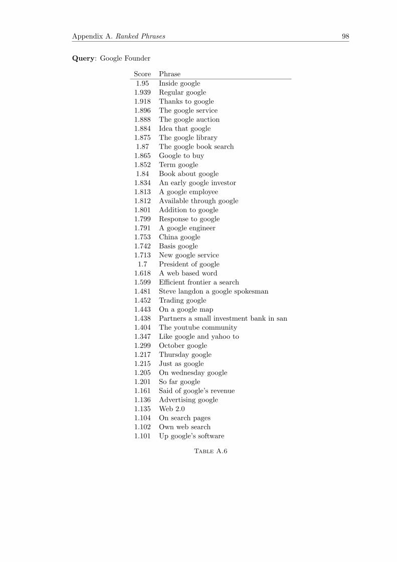
Appendix A. Ranked Phrases 98
Query: Google Founder
Score Phrase1.95 Inside google1.939 Regular google1.918 Thanks to google1.896 The google service1.888 The google auction1.884 Idea that google1.875 The google library1.87 The google book search1.865 Google to buy1.852 Term google1.84 Book about google1.834 An early google investor1.813 A google employee1.812 Available through google1.801 Addition to google1.799 Response to google1.791 A google engineer1.753 China google1.742 Basis google1.713 New google service1.7 President of google
1.618 A web based word1.599 Efficient frontier a search1.481 Steve langdon a google spokesman1.452 Trading google1.443 On a google map1.438 Partners a small investment bank in san1.404 The youtube community1.347 Like google and yahoo to1.299 October google1.217 Thursday google1.215 Just as google1.205 On wednesday google1.201 So far google1.161 Said of google’s revenue1.136 Advertising google1.135 Web 2.01.104 On search pages1.102 Own web search1.101 Up google’s software
Table A.6

Appendix B
Grouped Phrases
Query: Ronald Reagan
Saturday about the former presidentThe nation pauses to remember a presidentA president or former presidentFormer president’s funeral and a relatedFormer president authorizedCongress about the iran armsIran arms sales and efforts to aidThe arms sales and contra aidPoindexter is accused of five criminal chargesPoindexter’s chief defense lawyerHe faces five criminal chargesHis private diaries to john m. poindexterPoindexter’s lawyers haveReagan’s videotaped testimonyGovernor reagan his rise to powerReagan legacy projectKnown as ron is formally ronald prescott reaganMourning reagan and weighing his legacyReagan’s kitchen cabinetReagan’s biographerThe real reagan according to deaverReagan’s politicsReagan’s coffinReagan representsReagan was bornReagan’s testimony wasI now begin the journeyThe journey that will lead meThe reagan biographyTo the reagan library
Table B.1
99

Appendix B. Grouped Phrases 100
Query: Bill Gates
Barbarians led by bill gates the chairmanMicrosoft executives includingMicrosoft from the insideMicrosoft and its chairman bill gatesGates the microsoft corporationYear the bill and melindaBill gates the billionaireGates foundation in seattleGates foundation and george sorosBill gates and microsoftLike bill gates microsoftMelinda gates foundation gaveGates foundation has givenThe gates learning foundationGates a founder of microsoftA microsoft sponsored conferenceWhere bill gates and his wifeMicrosoft comparedMicrosoft’s founder bill gatesMicrosoft’s imageThe carnegie corporation the bill and melindaGates brokeThat the gates foundationGates’s softwareGates’s fortuneMelinda gates foundation and george soros sThe chairman of microsoft bill gatesIncluding the bill and melindaOf his $44 billion fortuneWife susan thompson buffettGates and buffettGates spentGates the world’s richestThe information highway cd romOn the information highway cd rom includedGates is rightGates’s retirementGates’s investmentGates’s managementOperations threaten human lifeWoman contends with a man who brutally attackedMan whose diamond mining operations threaten
Table B.2
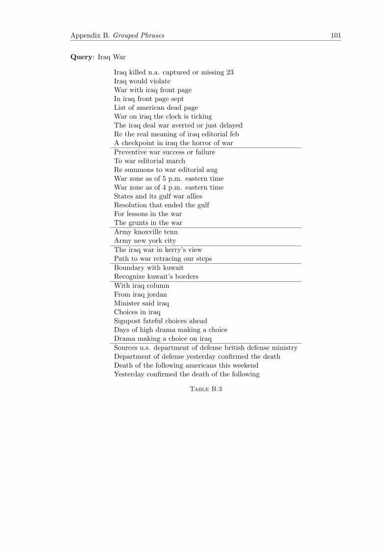
Appendix B. Grouped Phrases 101
Query: Iraq War
Iraq killed n.a. captured or missing 23Iraq would violateWar with iraq front pageIn iraq front page septList of american dead pageWar on iraq the clock is tickingThe iraq deal war averted or just delayedRe the real meaning of iraq editorial febA checkpoint in iraq the horror of warPreventive war success or failureTo war editorial marchRe summons to war editorial augWar zone as of 5 p.m. eastern timeWar zone as of 4 p.m. eastern timeStates and its gulf war alliesResolution that ended the gulfFor lessons in the warThe grunts in the warArmy knoxville tennArmy new york cityThe iraq war in kerry’s viewPath to war retracing our stepsBoundary with kuwaitRecognize kuwait’s bordersWith iraq columnFrom iraq jordanMinister said iraqChoices in iraqSignpost fateful choices aheadDays of high drama making a choiceDrama making a choice on iraqSources u.s. department of defense british defense ministryDepartment of defense yesterday confirmed the deathDeath of the following americans this weekendYesterday confirmed the death of the following
Table B.3

Appendix B. Grouped Phrases 102
Query: Brad Pitt
The hectic murky action sequencesTo a sprawling oddly lighthearted actionIn movies today and msOf this film takes placeS grimly powerful third filmWith such feeling and intelligenceA pair of california homicide detectives msNew film about a pairHis 1995 film the crossingAnd intelligence that you forgive the filmHis movies from the 1970And cigarettes starring cate blanchettThe gift starring cate blanchettIn various degrees of midnightNew movie is a sleek expensive lookingThe movie a rare touchA movie that glows in various degreesA movie for the wholeThe lambs is a movieA centuries old monster fighterThe title character a centuriesAs routine and familiar as the titleFrom a book by friedrich drrenmattBy friedrich drrenmatt reunites himThe supporting cast especially mrA cast that includes ray liotta garyWho serves up a castThat the titular figure unleashes mitchellA shaggy dog story mitchell
Table B.4

Appendix B. Grouped Phrases 103
Query: Afghanistan
With taliban and qaedaA taliban commander mullahWhen the taliban ruledOut taliban and al qaedaA taliban forceMonths the taliban pushedLeader mullah muhammad omar isThe taliban who were oustedThe whereabouts of mullahWhich the taliban hadThe taliban may beTo convene a loya jirgaBy a loya jirgaMajor afghan guerrillaOf the pakistan based guerrillaThe seven rebel partiesThe seven major guerrillaBased guerrilla partiesIndia iran and russiaThe northern alliance delegationMake up the northern alliance genThe so called northern allianceThe alliance of sevenIn eastern kunar provinceCapital of kunar provinceCapital of oruzgan provinceOf parwan provinceThe northern province of kunduzReaching pakistanAfghanistan the associated pressIntelligence officials in pakistanFor refugees in pakistanThe afghan press agencyMilitary intelligence agency the inter servicesMillion afghan refugees who haveWith zahir shahOf king mohammad zahir shahSaid the former kingDiego cordovez an ecuadoreanUnited nations mediator diego cordovez
Table B.5

Appendix B. Grouped Phrases 104
Query: Google Founder
At google in mountain viewCo founder larry pageTo search engineWith google mapsWaiting for google mrHow google and its rivalsOn its google printBy google last yearOf what google doesBy google and other internetAn early google investorA google engineerOn a google mapGoogle’s co foundersLarry page a co founderGoogle’s search technologyGoogle’s strategyGoogle’s biggestGoogle’s latestGoogle’s indexGoogle’s listWith the search engine giantGoogle that itIf google isTo acquire youtubeContent on youtubeBillion acquisition of youtubeThe youtube communityTo sell radio adsAds with graphicsDisplays adsSites that display its adsThe founders larryThe pay per click modelAcquired overtureAdvertising supported web servicesAnd overture servicesThe adsense
Table B.6
Bibliography
[1] Google traffic stats on alexa. http://www.alexa.com/siteinfo/google.com. Last
accessed, November 2009.
[2] Facebook lexicon. http://www.facebook.com/lexicon. Last accessed, November
2009.
[3] Google search options. http://www.google.com/support/websearch/bin/
answer.py?hl=en&answer=142143. Last accessed, November 2009.
[4] Mechanical turk. https://www.mturk.com. Last accessed, November 2009.
[5] New york times annotated corpus. http://corpus.nytimes.com. Last accessed,
April 2009.
[6] Penn treebank tag-set. http://www.cis.upenn.edu/~treebank. Last accessed,
November 2009.
[7] Penn treebank tag-set examples. http://www.comp.leeds.ac.uk/amalgam/
tagsets/upenn.html. Last accessed, November 2009.
[8] Stanford parts-of-speech tagger. http://nlp.stanford.edu/software/tagger.
shtml. Last accessed, November 2009.
[9] University of glasgow stop-word list. http://www.dcs.gla.ac.uk/idom/ir_
resources/linguistic_utils/stop_words. Last accessed, July 2009.
[10] Website optimization. http://www.websiteoptimization.com. Last accessed, Oc-
tober 2009.
[11] Weka 3: Data mining software in java. http://www.cs.waikato.ac.nz/ml/weka.
Last accessed, November 2009.
[12] Wordle. http://www.wordle.net, . Last accessed, November 2009.
[13] Wordnet lexical database. http://wordnet.princeton.edu, . Last accessed,
November 2009.
105

Bibliography 106
[14] Helena Ahonen. Knowledge discovery in documents by extracting frequent word
sequences. Library Trends, 48(1), 1999.
[15] Nilesh Bansal and Nick Koudas. Blogscope: a system for online analysis of high
volume text streams. Proceedings of the 33rd international conference on Very large
data bases, pages 1410–1413, 2007.
[16] Srikanta Bedathur, Klaus Berberich, Jens Dittrich, Nikos Mamoulis, and Gerhard
Weikum. Interesting-phrase mining for ad-hoc text analytics. PVLDB, 2010 (to
appear).
[17] F. J. Damerau. A technique for computer detection and correction of spelling errors.
Communications of the ACM, 7(3):171–176, 1964.
[18] John J. Darragh, Ian H. Witten, and Mark L. James. The reactive keyboard: A
predictive typing aid. Computer, 23(11):41–49, November 1990.
[19] Micah Dubinko, Ravi Kumar, Joseph Magnani, Jasmine Novak, Prabhakar Ragha-
van, and Andrew Tomkins. Visualizing tags over time. International World Wide
Web Conference, 1(2):193–202, August 2007.
[20] Ronald Fagin, R. Guha, Ravi Kumar, Jasmine Novak, D. Sivakumar, and An-
drew Tomkins. Multi-structural databases. Proceedings of the twenty-fourth ACM
SIGMOD-SIGACT-SIGART symposium on Principles of database systems, pages
184–295, 2005.
[21] R. W. Hamming. Error detecting and error correcting codes. Bell System Technical
Journal, 29(2):147–16, 1950.
[22] Akihiro Inokuchi and Koichi Takeda. A method for online analytical processing of
text data. Conference on Information and Knowledge Management archive, pages
455–464, 2007.
[23] Steven Keith, Owen Kaser, and Daniel Lemire. Analyzing large collections of elec-
tronic text using olap. Technical Report TR-05-001, UNBSJ CSAS, June 2005. URL
http://www.daniel-lemire.com/fr/documents/publications/tr05-001.pdf.
[24] Jon Kleinberg. Bursty and hierarchical structure in streams. International Confer-
ence on Knowledge Discovery and Data Mining, pages 91–101, August 2002.
[25] Tobias Leidinger. Entwicklung von back-end und testkonsole fur “phrase search
and analytics”, 2009.
[26] Brian Lent, Rakesh Agrawal, and Ramakrishnan Srikant. Discovering trends in text
databases. Knowledge Discovery and Data Mining, KDD, pages 227–230, 1997.

Bibliography 107
[27] Vladimir I. Levenshtein. Binary codes capable of correcting deletions, insertions,
and reversals. Soviet Physics Doklady, 10(8):707–710, 1966.
[28] Edward M. McCreight. A space-economical suffix tree construction algorithm. IEEE
Transactions on Knowledge and Data Engineering archive, 23(2):262–272, April
1976.
[29] Arnab Nandi and H. V. Jagadish. Effective phrase prediction. Proceedings of the
33rd international conference on Very large data bases, pages 219–230, 2007.
[30] Sven Obser. Entwicklung eines web-frontends fur “phrase search and analytics”,
2009.
[31] Alkis Simitsis, Akanksha Baid, Yannis Sismanis, and Berthold Reinwald. Multidi-
mensional content exploration. PVLDB, 1(1):660–671, March 2008.
[32] Ian H. Witten, Gordon Paynter, Eibe Frank, Carl Gutwin, and Craig G. Nevill-
Manning. Kea: Practical automatic keyphrase extraction. Proceedings of Digital
Libraries, November 1999.