Ecological Modelling, 35 (1987) 211-226 211 Elsevier Science Publishers B.V., Amsterdam - Printed in The Netherlands

QUALITATIVE MODEL OF EUTROPHICATION IN MACROPHYTE LAKES

A.A. VOINOV and A.P. TONKIKH

Laboratory of Mathematical Ecology, Computer Center of the U.S.S.R. Academy of Sciences, Moscow I17333 (U.S.S.R.)

(Accepted 25 March 1986)

ABSTRACT

Voinov, A.A. and Tonkikh, A.P., 1987. Qualitative model of eutrophication in macrophyte lakes. Ecol. Modelling, 35: 211-226.

A model is proposed for a qualitative representation of ecosystem dynamics in a macrophyte water body. The model variables are the concentrations of phytoplankton, macrophytes, nutrients, detritus and dissolved oxygen. By methods of qualitative theory of differential equations the model steady-state dynamics are studied (the 'quasi-stationary' process). The resulting evolution of the water body is in good agreement with the existing ideas about the succession of vegetation types under increasing nutrient load.

INTRODUCTION

To give a theoretical analysis of processes in ecosystems it may be fruitful to use simple mathematical models, containing just a few aggregated varia- bles and allowing an analytical treatment, but still giving a qualitatively correct representation of basic processes in ecosystems. Moiseev and Svirezhev (1979) suggested to term such models minimal models, stressing that they are to grip a certain basic 'minimal ' structure, which is responsible for the most essential dynamic ecosystem processes. Note that there is obviously no unique mathematical formalization of the minimal structure and therefore there may be several minimal models for each ecological system.

Earlier simple dynamic models were proposed for the eutrophication process is freshwater ecosystem (Voinov and Svirezhev, 1981, 1984). They gave a qualitative account of variations in phytoplankton concentrations in a lake under the impact of varying anthropogenic loads. The role of macrophytes, both submerged and emerged, is essentially different from the

0304-3800/87/$03.50 © 1987 Elsevier Science Publishers B.V.

212

ALGAEo

1 2

3 6

DETRITUS L

-I s r

i

41

7

Fig. 1. Flow diagram of material in a lake ecosystem. Numbers indicate: 1, 2 -- nutrient uptake by phytoplankton, and macrophytes, respectively; 3, 4 -- mortality of phytoplankton, and macrophytes, respectively; 5 -- destruction; 6 -- uptake of nutrients from sediments by macrophytes; 7 -- reaeration. Broken lines show 'information' flows.

role of phytoplankton, as their appearance in the lake noticeably affects the total system dynamics. It is known that the macrophyte stage is very

• important in the life-cycle of fresh-water bodies; consequently the ecological role of macrophytes should be taken into account when studying the long-term lake dynamics.

The lake ecosystem is represented by some very simple models, described by systems of ordinary differential equations with variables representing concentrations of phytoplankton and macrophytes, competing for nutrients. The material cycle is closed by the variable which stands for the concentra- tion of detritus (Fig. 1). By methods of qualitative theory of differential equations the model steady-state dynamics are studied (the 'quasi-sta- tionary' process). The predicted evolution of the water body turns to be in good agreement with the existing ideas about the succession of vegetation types under an increasing nutrient load. Proceeding from some general ecosystem characteristics one may define which pathway the lake evolution is most likely to follow.

213

MACROPHYTES IN LAKE ECOSYSTEMS

Both submerged and emergent macrophytes, unlike the rest of the water vegetation and phytoplankton, are attached to the bot tom and can uptake nutrients from the sediments, the settled detritus, etc. Submerged macro- phytes are provided with nutrients partly from the bot tom and partly by those dissolved in the water. The emergent ones get practically all their nutrition from the bottom. This source of nutrition gives emergent macro- phytes a certain competitive advantage with phytoplankton. Furthermore, macrophytes occupy the shores of water bodies and are the first to catch the allochthonous nutrients. Phytoplankton, on the other hand, reaching suffi- ciently high concentrations, can suppress submerged macrophytes depriving them of light. However, macrophytes can develop for some time in the dark due to so-called 'dark respiration' uptake of reserves; this ability to accu- mulate nutrients is a distinctive feature of macrophytes. While the aerial part of the emerging macrophytes dies every year, their root system lives for a number of years, with the ratio of the root biomass to the rest of the plant being close to unity.

It is hard to take account of all these properties in the framework of a minimal model, and they are hardly equally significant when analyzing the long-term qualitative lake dynamics. Analysis of this kind for the eutrophi- cation process has been performed in a paper by Voinov and Svirezhev (1984) where the dynamics of phytoplankton, nutrients, detritus and dis- solved oxygen have been modelled. The choice of these variables has been based on some general biological speculations as well as asymptotic analysis of material transformations in freshwater ecosystems. To consider the mac- rophyte dynamics, let us add one more variable - - the concentration of macrophytes - - and rewrite the model in the following form:

d = e ~ n a - p a

rh = ( f i n + Ns)(1 - r n / M ) m - y m

it = 8 ( x ) s - a n a - f i n ( 1 - m / M ) m (1)

= o a + "I'm - 8 ( x ) s - Ns(1 - m / M ) m

2 = k ( x s - x ) + ~a + f m - o 8 1 ( x ) s

where a is phytoplankton concentration, m macrophyte concentration, n nutrient concentration, s detritus concentration, and x concentration of dissolved oxygen. The parameters in system (1) have the following sense: a is the uptake rate of nutrients by phytoplankton ((mg/1) -1 day- l ) , p phytoplankton mortality (day-1), k reaeration coefficient (day-1), assimila- tion coefficient, i.e. the 0 2 output in photosynthesis (mg O 2 mg x biomass

214

5~(X)

\\\ \ ~ ~x

52(x) I " ' 1

XAN X A

Fig 2. Destruction rate of dead organic material and recycling of nutrients as function of the dissolved oxygen concentration. Broken line shows the function for phosphorus limited ecosystems.

day-a) , o biochemical oxygen demand in destruction process (rag 0 2 mg t biomass), x s saturation concentrat ion of oxygen (mg/1), fl uptake rate of dissolved nutrients by macrophytes ((rag/l) -1 day - l ) , N uptake rate of nutrients of detritus by macrophytes ((mg/1) -1 day-a) , 3, macrophyte mortal i ty (day- l ) , ~" assimilation coefficient for the submerged part of macrophytes (mg O 2 mg -1 biomass day - t ) , M carrying capacity of the environment for macrophytes (mg/1); 3(x) (day -1) characterizes the rela- t ionship between the destruction rate of dead organic material (the recycling of nutrients) and the concentrat ion of dissolved oxygen and it takes the form of one of the two functions presented in Fig. 2. This model may be studied by methods of the qualitative theory of ordinary differential equations.

MODEL WITH EMERGING MACROPHYTES, NOT ACCOUNTING FOR CARRY- ING CAPACITY

Consider the special case when fl = 0, that is, macrophytes uptake nutri- ents only from the sediments. This is the kind of nutri t ion, which is specific to emerging macrophytes; they receive a negligibly small fraction of nutri- ents f rom the water. Since photosynthesis of emerging macrophytes dis- charges oxygen primarily into the atmosphere, we may suppose that ~ = 0. Also suppose that the carrying capacity of the environment by far exceeds the existing macrophyte concentrations, i.e. m / M = O. This assumpt ion is quite plausible for shallow water bodies, where macrophytes can cover the whole surface area.

For the first four equations in system (1) there exists the first integral:

a + m + n + s = A = constant (2)

215

Thus system (1) may be rewritten in the following form:

d = a ( B - m - a - s ) a rh = Nsm - ym g = p a + y m - 8 ( x ) s - N s m (3)

2 = k ( x s - X ) + l i a - o 6 t ( x ) s

where B = A - O/a. This system has three steady-state points:

(1) a 1 = 0 ; r n l = 0 ; s t = 0 ; n l=A; x l = x s

(2) a a = 8 ( x 2 ) B / ( 6 ( x 2 ) + p ) ; m 2 = 0 ;

s2=pB/ (8(x2)+O); n 2 = p / a

where x a is the solution to the equation:

k ( x s - x) + ~ a - o 61(x ) s = O (4)

with a = a 2 , s = s 2.

(3) a 3 = 6 ( x 3 ) V/pS; m 3 = B - Y ( 6 ( x 3 ) + P ) / S p ;

s 3 = y / N ; n 3 = p/ct

x 3 is again the solution to equation (4), which now takes the form:

k ( x s - - X3) -['- ~ 6 (X3) ~//p~'~ -- Or 61(X3) "y/~'~ = 0 (5)

For the second stationary point, which is just the same as the non-trivial equil ibrium in the model studied earlier (Voinoz and Svirezhev, 1984), it is easy to show that equation (4) has a unique positive root if 8 ( x ) = 61(x ). When the parameters satisfy the condit ion that ~ > oO we get x 2 > xs, which means that the lake becomes a source of oxygen. Otherwise xl ~< x s. For 8(x) = 82(x ) in the general case we cannot be sure that a root will exist in (4). Rewrite (4) as:

k(x~-x)(62(x)+p)+~ 62(x) B=opB 61(x ). The left-hand side here is a mono tone non-increasing function of x, denoted f l (x ) ; the r ight-hand side is an increasing function, f2(x). Since f l ( m ) < f 2 ( ~ ) , for a root to exist in (4) it is sufficient that fx(0) >f2(0), that is:

kxsp + 62(0)(~B + kx~) > 31(0 ) 3109 (6)

Note that since 32(0 ) >> 31(0 ) the latter condi t ion will hold for most of the real parameter values. The root will be localized in the interval [0, x J , if we addit ionally demand that f l (Xs)<f2(x~) , i.e. ~ 62 (Xs)<op 61(xs). This condi t ion is also most likely to hold, since 82(x~)<< 61(x~) and it will certainly hold when ~ < op.

216

k X s

(o'q>g)

6

O / k X s

7,(0-q-~)/¢

// / 6 (x)

X

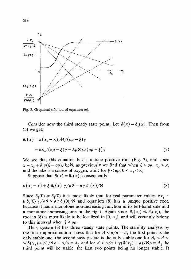
Fig. 3. Graphical solution of equation (6).

Consider now the third steady state point. Let 8 ( x ) = 31(x ). Then from (5) we get:

31(x ) = k ( x s - x ) p ~ / ( o p - ~ )~

= k x s / ( O p - ~ ) y - k p ~ x / ( o p - ~ ) y (7)

We see that this equation has a unique positive root (Fig. 3), and since x = xs + 813,(~ - o p ) / k p ~ , as previously we find that when ~ > oO, x3 > Xs and the lake is a source of oxygen, while for ~ < op, 0 < x 3 < x~.

Suppose that 8(x) = 32(x); consequently:

(Xs- x) 82(x) v/ps =or 3 (x)/s (8)

Since 32(0 ) >> 31(0 ) it is most likely that for real parameter values kx s + 32(0) "y/p~ > o7 81(0)/~ and equation (8) has a unique positive root,

because it has a monotone non-increasing function in its left-hand side and a monotone increasing one in the right. Again since 32(x~)<< 31(xs), the root in (8) is most likely to be localized in [0, x~], and will certainly belong to this interval when ~ < op.

Thus, system (3) has three steady state points. The stability analysis by the linear approximation shows that for A < p / o r = A 1 the first point is the only stable one, the second steady state is the only stable one for A1 < A < y(3(X3) -'[- p ) / N p -[- p / a -.~-A 2 and for A > p / a + y(8(x3) + p)/Np = A 2 the third point will be stable, the first two points being no longer stable. It

217

1 2 3

0 A I A 2

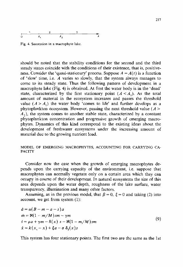
Fig. 4. Succession in a macrophyte lake.

should be noted that the stability conditions for the second and the third steady states coincide with the conditions of their existence, that is, positive- ness. Consider the 'quasi-stationary' process. Suppose A - -A( t ) is a function of 'slow' time, i.e. A varies so slowly, that the system always manages to come to its steady state. Thus the following pattern of development in a macrophyte lake (Fig. 4) is obtained. At first the water body is in the 'dead' state, characterized by the first stationary point (A <At) . As the total amount of material in the ecosystem increases and passes the threshold value (A > A1) the water body 'comes to life' and further develops as a phytoplankton ecosystem. However, passing the next threshold value (A > A2), the system comes to another stable state, characterized by a constant phytoplankton concentration and progressive growth of emerging macro- phytes. Dynamics of this kind correspond to the existing ideas about the development of freshwater ecosystems under the increasing amount of material due to the growing nutrient load.

MODEL OF EMERGING MACROPHYTES, ACCOUNTING FOR CARRYING CA- PACITY

Consider now the case when the growth of emerging macrophytes de- pends upon the carrying capacity of the environment, i.e. suppose that macrophytes can normally vegetate only on a certain area which they can occupy in course of their development. In natural ecosystems the size of this area depends upon the water depth, roughness of the lake surface, water transparency, illumination and many other factors.

Assuming, as in the previous model, that fl = 0, ~ = 0 and taking (2) into account, we get from system (1):

d = a ( B - m - a - s ) a

rh = b~(1 - m/M)srn - ym

~---pa + v r n - 8 ( x ) s - l ' l ( 1 - m / M ) s m

= k ( x s - x) + ~ a - o 81(x)s

(9)

This system has four stationary points. The first two are the same as the 1st

218

and the 2nd stationary points in the previous model. The 3rd point has the following form:

(3) a3=8(x3)(B- M+ ¢(B- M) 2 + 4"yM(~(x3)+ O)/NO) / 2 ( 8 ( x 3 ) + P ) ;

S 3 = P a 3 / 8 ( x 3 ) ; m 3 = M(I - " y S ( x 3 ) / a 3 ~ P ) ; n 3 --- P l o t

x 3 is found from equation (4). The 4th equilibrium is always negative. As in the previous model the

localization problem may be solved for roots of (4). The succession of steady states is the same as in the previous model. The threshold values of A also remain the same, coinciding with the positiveness conditions for the ap- propriate points. However the introduction of the environmental carrying capacity for macrophytes radically alters the dynamics of the 3rd steady state. When A grows from A 2 to M the ecosystem development is char- acterized by a progressive macrophyte growth and a slight increase of the phytoplankton biomass. When A passes the threshold value A = M and the total biomass grows further, the macrophyte biomass asymptotically ap- proaches M, while the concentrations of phytoplankton and detritus sharply start to grow (Fig. 5), i.e. the system steady state becomes characterized by a constant macrophyte biomass and a progressively growing phytoplankton population. It may be concluded that macrophytes play a role specified by a barrier-type function with respect to the nutrient load. After they reach a certain saturation level (for instance, when the cell accumulation of nutrients

15

tn

o Jcl

0 / / 2 0 Ja

I'll I l l ~,~

p IJ ~

i J#/I/'¢l I ¢1¢11 ( 10

0 OI • o ~3 13 2~ ~ Js 4a

Fig. 5. Phytoplankton (1) and macrophyte (2) dynamics under increasing nutrient load: a= 0.46, p = 0.12, 1,1=1.01, T =0.05, 8=0.42, M= 30.0, A3 = 0.49.

219

is at maximum or all the area suitable for vegetation is covered) they can no longer intercept the nutrient load and phytoplankton production is activated. An example is presented by the ecosystem dynamics in the macrophyte lake Sevan in Armenia. After a rapid release of water, when the carrying capacity of the environment for macrophytes was sharply reduced, phytoplankton immediately became the dominant primary producer in this lake (Pokrovskaya et al. 1983).

M O D E L W I T H S U B M E R G E D A N D E M E R G I N G M A C R O P H Y T E S

Let us suppose that by m we represent the aggregated biomass of submerged and emerging macrophytes. In this case it is difficult to specify the value of the carrying capacity and therefore macrophytes are considered to be independent of it. Aggregated macrophytes uptake nutrients both from the water body and from the bottom (Fig. 1), consequently now /3 :g 0. Additionally, submerged macrophytes produce photosynthetic oxygen in the water, so ~ 4: 0. Thus, taking (2) into account, we can write system (1) in the following form:

g t = a ( B - m - a - s ) a

rh = fl( A - a - m - s ) m + Nsm - ' g m

= p a + 3 , m - 3 ( x ) s - N s m

2 = k ( x s - x ) + ~ a + ~ m - o a l ( x ) s

(lO)

Let us find the steady state points in this system. The first two points remain unchanged:

(1)

(2)

a l = O ; m 1 = 0 ; s 1 = 0 ; n l = A ;

a z = 8 ( x 2 ) B / ( 3 ( x 2 ) + P); m 2 = 0 ;

s2=oB/(8(x2)+o); n2=o/ x 2 is a root to equation (4).

X 1 ~ X s

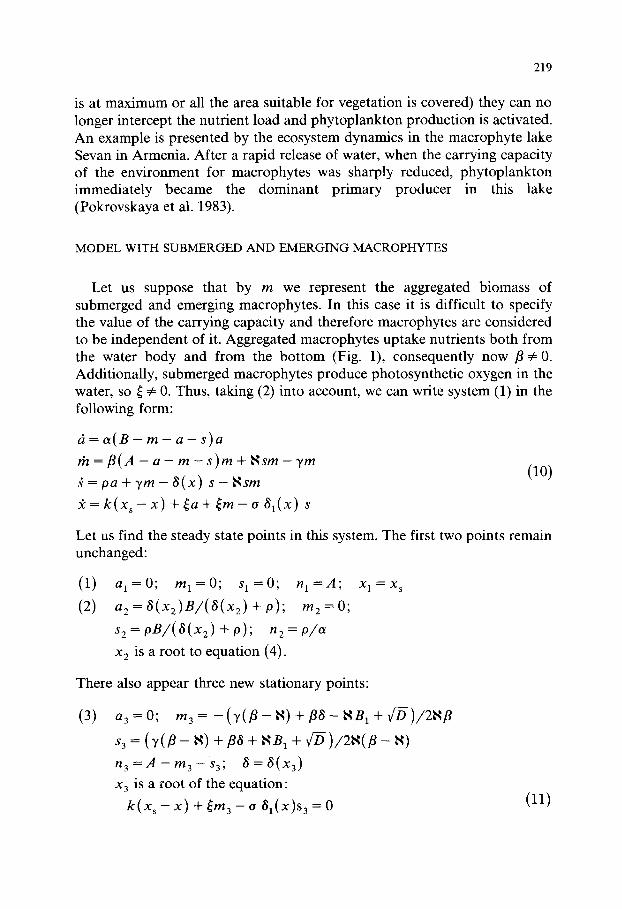
There also appear three new stationary points:

(3) a 3 = 0 ; m , = - ( y ( / 3 - N ) + / 3 3 - N B x+vr-D)/2Nfl

s 3 = ( - / ( /3- N) + 133 + NB 1 + v /D) /2N( /3- N)

n 3 = A - m 3 - s 3 ; 3 = 3 ( x 3 ) x 3 is a root of the equation:

k ( x s - x ) -t- ~m 3 - 0 31(x)s 3 -~- 0 (11)

220

(4) a 4 = 0 ; m4 = -- ( y ( / 3 -- ~ ) -b/3~ -- S B 1 - V ~ - ) / 2 ~ / 3

$4 = (T( /3 -- ~ ) "[- B ~ -]- b~B1 -- vr/))/2b~(/3 - b~)

n 4 = A - m 4 - s 4 ; 8 = 8 ( x 4 )

x 4 is found from equation (11) substituting m 4 and s 4.

Here the following notations have been used:

D = (V(/3 - N) -t--/38 + NB1) 2 - 4Nr ( f l - N)B 1

B 1 = /3A - T

(5) a s = ( a T - p f l ) ( a 8 + f l p ) / a p ~ ( a - B ) - f l B / ( a - B )

m s = - (aT - p f l ) ( p + 8 ) / p l ' ~ ( a - B ) - f l B / ( a - B )

ns = p / a ; ss = ( a T - - / 3 p ) / a ~ ; 8 = a ( x s )

x s is the solution to the equation:

k ( x s - x ) + ~ a + f r n - o S l ( x ) s = 0 (12)

when substituting as, m s and s s. Let us see when these points belong to the positive orthant of the phase

space. The 1st point is always positive. The 2nd point is positive for A > p / a = A x. It is easily shown that the third point is ecologically sensible only when

A2 = (3' + ~ ( x 2 ) ) / ~ < A < T//3 = A3

The condition Tb~ >/3(T + 8) should hold in this case. The condition for the 4th point is A > m i n { ( T + 6 ( x 4 ) / N , 3'//3)- And finally the 5th point is positive only when aT >/30 and min(A 4, As) < A < max(A 4, As), where:

A . = p/a + (a3, - / 3 p ) ( a ~ ( x s ) + / 3 p ) / a / 3 0 s

A s = p/a + ( a T - - / 3 p ) ( p + 8(xs))/apS

Notice that A 4 < A s when a </3 and vice versa. Moreover, for b~ >/3 another condition appears which follows from the demand that the discrimi- nant D be positive:

A 6 = (3' - 8 ) / ~ - 2~/383,(S - / 3 ) / S / 3

< A < (V - 8 ) / N - 2~//36T(N - / 3 ) / N / 3 = A 7

Another series of conditions may still appear from the expressions for the oxygen concentrations x i (i -- 2, 3, 4, 5).

Since it is hardly possible to study analytically the stability of all these points, we resort to numerical computer analysis. A special programme was

221

used to compute the roots of the characteristic polynomial for the linearized matrix. The model parameters have been estimated basing on data from literature (Jorgensen, et al., 1978; Bikbulatov and Bikbulatova, 1979; Yeli- zarova, 1982).

Calculations have been performed for all kinds of combinations of the following parameter values:

a = 0.5 1.0 2.0 p = 0.05 0.1 0.15

/3 = 0.005 0.01 0.1

N = 0.05 0.1 0.5 ~, = 0.001 0.005 0.01

k = 0.1 1.0 = 0.005 0.01 0.05

~ '=0.0005 0.001 0.005

o = 0.018 0.05 0.08 XAH = 1.0 1.5 2.0

X s ---- 2.2 2.5 3.0

X 6 = 10.0

3 = 0 . 0 4

3.0 0.3

0.5

1.0 0.03

0.1

0.01 0.25 0.4

First the model was analyzed for 3 ( x ) = constant, that is assuming the ecodynamics to be independent of oxygen concentrations. As in the preced- ing models the values A i (i = 1, . . . ,7) turned out to be thresholds in the succession of the system stable regimes. The following scheme of calcula- tions was followed: (1) compute the threshold points Ai; (2) divide each interval between two thresholds [A~, Al] into ten parts:

if A t = minAi, then A k = 0; if A k = maxA~, then A l = 2A k i i

(3) for A fixed at one of the intermediate interval points, compute the stationary values for a, m, s and n and study the stability of the point;

(4) pass to the next intermediate interval point and go to 3. Numerical model analysis for different combinations of parameter values

leads us to the conclusion that, generally, all the variants of ecosystem succession under the impact of growing material amount A may be reduced to the patterns presented in Fig. 6. The possible domains of stability of the stationary points for two sets of parameters are presented in Fig. 7. It also turned out that the value of 3 has no effect upon the development of the alternating stable ecosystem states. Since $ is determined by the steady state oxygen concentration x*, we may think that within the framework of the

222

1 i

A~ 2

A 5

5 5 5 5 4 J i i i I . -

A 2 A 7 A 3 A 4 A

(a)

o % 1 i

A2

1

A1 2 i 2~ 4

• 4 7

(b)

5 , 4 4 4 i i i

• 4 5 A 4 /I 3

1 2 2 2 2 5 4 t ~ t i ~ J ! , , 4

A1 A 7 A 3 A 2 A 5 A 4 (C)

1 i

A2

1 1,4

A7

4 4 4 4 t i i I L

A3 A4 A 5 A1 A

(d)

I i

AI 2

A 3

2 I 2 , 4 4 4

(e)

1 2

A3

2 5 5 4

(f)

I 1

A 7

1 4 4 4 4 i i i i - -

A 3 A 5 A, A 2 VA (g)

1 1

A1

2 5 5 4 4

(h)

Fig. 6. Different ways of lake evolution with submerged and emerging macrophytes. Figures indicate the numbers of equilibrium points which are stable in the given interval.

model oxygen dynamics has no qualitative effect upon the succession, but only changes the quantitative values of the thresholds A i between different steady states.

To study the dynamics of oxygen, the function 6(x) was approximated by a piecewise linear one and the following scheme of calculations was chosen: (1) choose a sufficiently small value A; (2) by method of halving the interval solve equation (4) with substituted a 2

and s 2 to get the value x2; (3) similarly solve equations (8) and (9) to find the values x3, x 4 and xs;

1.48

1.11 -

0.74-

0,37 -

o.o

(a )

t I

0~12 0.24 0.36 0.48 0.60

223

0.10

0 .075

0 , 0 5 0

0 . 0 2 5

0.0

(b )

0:12 0.24 0.'36 O.ZI8 0 : 6 0 ~

Fig. 7. Domains of stability of steady state points. I - - 1st point is stable, II - - 2nd point is stable, III - - 4th point is stable, IV - - 5th point is stable. (a) p = 0.05, fl = 0.05, ~ = 0.13, 3' = 0.01, 8 = 0.019. (b) p = 0.07, fl = 0.08, ~ =1.00, 3' = 0.01, 8 = 0.019.

(4) c o m p u t e the co r re spond ing values of a, s, m and n; (5) increase A by AA = 1 and go to 2 if A is smaller t han the preset

pa r a me te r A ma~- It turns out tha t oxygen concen t ra t ions that co r r e spond to posi t ive s table

po in ts take on plausible values close to x S. W h a t m a y be the in t e rp re t a t ion of the ob t a ined var iants of ecosys tem

deve lopmen t? As in the first mode l vers ion the evolu t ion starts with the state charac te r ized by absence of life in the ecosys tem ( l s t point) and eventua l ly comes to the state in which p h y t o p l a n k t o n loses in compet i t ion , declines to ex t inc t ion and mac rophy t e s domina t e the lake (4th point) . Be tween these states the ecosys tem m a y go th rough a series of s table s teady states. F igure 6 demons t r a t e s the succession of stable states in the system for vary ing mode l pa rame te r s and externa l nu t r i en t load. Mos t typical is the succession:

1 ~ 2 ~ 5 ~ 4

224

s t o t e 4

s t o t e 2

0 A 4 A 5

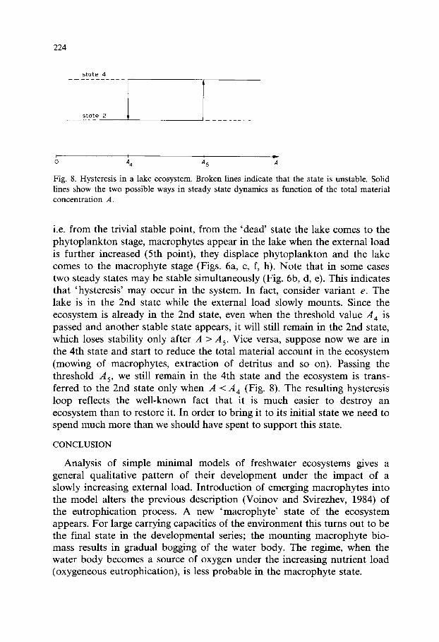
Fig. 8. Hysteresis in a lake ecosystem. Broken lines indicate that the state is unstable. Solid lines show the two possible ways in steady state dynamics as function of the total material concentration A.

i.e. from the trivial stable point, from the 'dead' state the lake comes to the phytoplankton stage, macrophytes appear in the lake when the external load is further increased (5th point), they displace phytoplankton and the lake comes to the macrophyte stage (Figs. 6a, c, f, h). Note that in some cases two steady states may be stable simultaneously (Fig. 6b, d, e). This indicates that 'hysteresis' may occur in the system. In fact, consider variant e. The lake is in the 2nd state while the external load slowly mounts. Since the ecosystem is already in the 2nd state, even when the threshold value A 4 is passed and another stable state appears, it will still remain in the 2nd state, which loses stability only after A > A 5. Vice versa, suppose now we are in the 4th state and start to reduce the total material account in the ecosystem (mowing of macrophytes, extraction of detritus and so on). Passing the threshold As, we still remain in the 4th state and the ecosystem is trans- ferred to the 2nd state only when A < A 4 (Fig. 8). The resulting hysteresis loop reflects the well-known fact that it is much easier to destroy an ecosystem than to restore it. In order to bring it to its initial state we need to spend much more than we should have spent to support this state.

CONCLUSION

Analysis of simple minimal models of freshwater ecosystems gives a general qualitative pattern of their development under the impact of a slowly increasing external load. Introduction of emerging macrophytes into the model alters the previous description (Voinov and Svirezhev, 1984) of the eutrophication process. A new 'macrophyte ' state of the ecosystem appears. For large carrying capacities of the environment this turns out to be the final state in the developmental series; the mounting macrophyte bio- mass results in gradual bogging of the water body. The regime, when the water body becomes a source of oxygen under the increasing nutrient load (oxygeneous eutrophication), is less probable in the macrophyte state.

225

When the carrying capacity is bounded, the macrophyte stage is char- acterized by limited macrophyte growth. Further increase in the external load again results in growing phytoplankton concentrations, that is, in 'phytoplanktonic eutrophication' of the water body.

Some refinement of the model, by the introduction of submerged macro- phytes, makes the analysis considerably more complex. Computer simula- tions show that though the general lake succession remains the same - - f rom a 'dead' lake towards a macrophyte one - - there is a variety of intermediate stages. Their sequence depends upon concrete parameter values specifying the ecosystem. However, the study of the refined model reveals some drawbacks of the adopted conceptional scheme. As a result of the aggrega- tion of submerged and emerging macrophytes in one block, macrophytes always displace phytoplankton in competition. This is actually so if we take into account competition for nutrients only. In competition for light phyto- plankton enjoys more favourable conditions in comparison with submerged macrophytes and displaces them when the nutrient load is increased. To represent this mechanism in a model we need to take into account the light limitation of vegetation growth, which in this case defines the carrying capacity for macrophytes. Submerged and emergent macrophytes will have to be disaggregated, making the qualitative analysis much more difficult. One may expect only a numerical study within the framework of a more complicated simulation model.

In the model the threshold values of A, indicating the beginning of the macrophyte stage in the lake development, usually were rather large. There- fore we may think that this stage presents the period of overgrowing and bogging of the lake. In this case the model results give a sufficiently adequate representation of the qualitative development process in natural lake ecosystems. Thus, using simple models, one may deduce interesting, not obvious intuitively, regimes in lake dynamics (hysteresis, 'oxygen eutrophi- cation'), and find the conditions for the model parameters necessary for their origination. It should be noted that qualitative models in ecology, as a rule, may be related to one of the two classes. On the one hand, it is the models which emanate from a mathematically interesting result which is then interpreted in appropriate ecological terms. On the other hand there is the concept of minimal models which are essentially derived from the ecological object by 'minimizing' it to such an extent that it may be studied qualitatively though not necessarily analytically. Usually this gives no new mathematical results, but leads to a more ecologically justified representa- tion.

ACKNOWLEDGEMENT

The authors are extremely grateful to Prof. Yu.M. Svirezhev for his ideas and helpful discussions.

226

REFERENCES

Bikbulatov, E.S. and Bikbulatova, E.M., 1979. Decay rate of the organic material of dead phytoplankton. In: Microbiological and Chemical Processes of Destruction of Organic Material in Water Bodies. Nauka, Leningrad, pp. 213-224 (in Russian).

Jorgensen, S.E. (Editor-in-chief), Friis, M.B., Henriksen, J., Jorgensen, L.A. and Mejer, H.F. (Editors), 1978. Handbook of Environmental Data and Ecological Parameters. ISEM, Vaedose, Denmark, 1162 pp.

Moiseev, N.N. and Svirezhev, Yu.M., 1979. Conceptional biosphere model. Bull. U.S.S.R. Acad. Sci., 1979 (2): 47-58 (in Russian).

Pokrovskaya, T.N., Mironova, N.Ya. and Shilkrot, G.S., 1983. Macrophyte Lakes and their Eutrophication. Nauka, Moscow, 152 pp. (in Russian).

Voinov, A.A. and Svirezhev, Yu.M., 1981. Stability in a simple model of an aqueous ecosystem. J. Gen. Biol., 42:936-940 (in Russian with English summary).

Voinov, A.A. and Svirezhev, Yu.M., 1984. A minimal model of eutrophication in freshwater ecosystems. Ecol. Modelling, 23: 277-292.

Yelizarova, V.A., 1982. Some data on reproduction rates of planktonic algae in the litoral of the Rybinsk reservoir. In: A.V. Monakov (Editor), Hydrobiological Characteristics of Reservoirs of the Volga Basin, Nauka, Leningrad, pp. 57-68 (in Russian).