On the Stability of the Passive Dynamics of

Quadrupedal Running with a Bounding Gait1

Ioannis Poulakakis2, Evangelos Papadopoulos3, and Martin Buehler4

poulakas@eecs.umich.edu|egpapado@central.ntua.gr|buehler@BostonDynamics.com

2Control Systems Laboratory

Department of Electrical Engineering and Computer Science

The University of Michigan

Ann Arbor, MI 48109, U.S.A.

3Department of Mechanical Engineering

National Technical University of Athens

Athens, 15780, Greece

4Boston Dynamics

Cambridge, MA 02139, U.S.A.

Submitted to the

International Journal of Robotics Research as a Full Paper

September 2005, Accepted March 2006

1 Portions of this paper have previously appeared in conference publications [28] and [30]. The first and third

authors were with the Centre for Intelligent Machines at McGill University when this work was performed. Address

all correspondence related to this paper to the first author.

2

ABSTRACT

This paper examines the passive dynamics of quadrupedal bounding. First, an unexpected

difference between local and global behavior of the forward speed versus touchdown angle in the

self-stabilized Spring Loaded Inverted Pendulum (SLIP) model is exposed and discussed. Next,

the stability properties of a simplified sagittal plane model of our Scout II quadrupedal robot are

investigated. Despite its simplicity, this model captures the targeted steady state behavior of

Scout II without dependence on the fine details of the robot structure. Two variations of the

bounding gait, which are observed experimentally in Scout II, are considered. Surprisingly,

numerical return map studies reveal that passive generation of a large variety of cyclic bounding

motion is possible. Most strikingly, local stability analysis shows that the dynamics of the open

loop passive system alone can confer stability of the motion! These results can be used in

developing a general control methodology for legged robots, resulting from the synthesis of

feedforward and feedback models that take advantage of the mechanical system, and might

explain the success of simple, open loop bounding controllers on our experimental robot.

KEY WORDS – Passive dynamics, bounding gait, dynamic running, quadrupedal robot.

1 INTRODUCTION

Mobility and versatility are the most important reasons for building legged robots, instead of

wheeled and tracked ones, and for studying legged locomotion. Animals exhibit impressive

performance in handling rough terrain, and they can reach a much larger fraction of the earth

landmass on foot than existing wheeled vehicles. Most mobile robotic applications can benefit

from the improved mobility and versatility that legs offer.

Early attempts to design legged platforms resulted in slow moving, statically stable

robots; these robot designs are still the most prevalent today, see [5] for a survey. In this paper,

however, we restrict our attention to dynamically stable legged robots. Twenty years ago Raibert

set the stage with his groundbreaking work on dynamic legged robots by introducing a three-part

controller for stabilizing running on his one-, two-, and four-legged machines, [31]. His

controllers, although very simple, resulted in high performance, robust running with different

gaits, such as the trot, the pace, and the bound. Inspired by Raibert’s work, Buehler and his

3

collaborators at McGill’s Ambulatory Robotics Laboratory (ARL) designed and built power

autonomous one-, four-, and six-legged platforms, which demonstrate walking and running in a

dynamic fashion; see [7] for an overview. Minimal actuation, coupled with a suitably designed

mechanical system featuring compliant legs, and simple control laws that excite the natural

dynamics of the mechatronic system are the underlying fundamental principles exemplified by

ARL’s robots.

Other design and control approaches for dynamically stable running robots have been

proposed, including the Patrush and Tekken robotic quadrupeds by Kimura and his collaborators,

[13], [20]. Based on principles from neurobiology, they implemented bounding by transitioning

from pronking in Patrush by combining compliant legs with a neural oscillator network, [20].

More recently, Fukuoka et al. proposed a controller based on a Central Pattern Generator (CPG)

that alters its active phase based on sensory feedback and results in adaptive dynamic walking on

irregular terrain, [13]. Following a different design approach, Cham et al. introduced Sprawlita, a

spectacularly robust dynamic hexapod, capable of running with speeds over four body lengths

per second on irregular terrains with hip height obstacles, [10]. The authors employed a novel

manufacturing technique to construct a biomimetic mechanism with actuators, sensors and

wiring embedded in the robot’s body and limbs.

Despite their morphological and design differences these robots walk and run using

control laws without intense feedback. For instance, recent research on our quadrupedal robot

Scout II (Fig. 1) demonstrated that simple controllers, requiring only touchdown detection and

local feedback from motor encoders, can be used to stabilize running, [29], [30]. These

controllers simply position the legs at a fixed touchdown angle during the flight phase, and result

in stable bounding with speeds up to 1.3 m/s. A slightly modified control strategy was

successfully implemented on Scout II to result in the first ever reported robot gallop gait, [30],

[38]. Similar design and control ideas as found in Scout II have subsequently been implemented

to generate bounding in a modified (one actuator per leg) version of the SONY AIBO dog, [40],

and in the one-actuator-per-leg hexapedal RHex, [8] (see [32] for design and control details).

Recently RHex traversed irregular terrain with speeds over five body lengths per second and

reduced specific resistance, [39]. Once again the controller employs only local feedback from

encoders, necessary for the leg recirculation strategy, while the parameters for some of its gaits

are determined via Nelder-Mead optimization, [39].

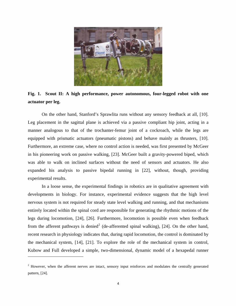
Fig. 1. Scout II: A high performance, power autonomous, four-legged robot with one

actuator per leg.

On the other hand, Stanford’s Sprawlita runs without any sensory feedback at all, [10].

Leg placement in the sagittal plane is achieved via a passive compliant hip joint, acting in a

manner analogous to that of the trochanter-femur joint of a cockroach, while the legs are

equipped with prismatic actuators (pneumatic pistons) and behave mainly as thrusters, [10].

Furthermore, an extreme case, where no control action is needed, was first presented by McGeer

in his pioneering work on passive walking, [23]. McGeer built a gravity-powered biped, which

was able to walk on inclined surfaces without the need of sensors and actuators. He also

expanded his analysis to passive bipedal running in [22], without, though, providing

experimental results.

In a loose sense, the experimental findings in robotics are in qualitative agreement with

developments in biology. For instance, experimental evidence suggests that the high level

nervous system is not required for steady state level walking and running, and that mechanisms

entirely located within the spinal cord are responsible for generating the rhythmic motions of the

legs during locomotion, [24], [26]. Furthermore, locomotion is possible even when feedback

from the afferent pathways is denied2 (de-afferented spinal walking), [24]. On the other hand,

recent research in physiology indicates that, during rapid locomotion, the control is dominated by

the mechanical system, [14], [21]. To explore the role of the mechanical system in control,

Kubow and Full developed a simple, two-dimensional, dynamic model of a hexapedal runner 2 However, when the afferent nerves are intact, sensory input reinforces and modulates the centrally generated

pattern, [24].

4

5

(death-head cockroach, Blaberous discoidalis), [21]. The model had no equivalent of nervous

feedback among any of its components and it was found to be inherently stable. This work first

revealed the significance of mechanical feedback in simplifying neural control, by demonstrating

that stability could result from leg moment arm changes alone. Therefore, one can assume that

intense control action relying on complex feedback from a multitude of sensory receptors is not

necessary to generate and sustain walking and running.

In an attempt to set the basis for a systematic approach in studying legged locomotion

Full and Koditschek introduced the templates and anchors modeling and control hierarchy, [14].

Schmitt and Holmes proposed the Lateral Leg Spring (LLS) template to analyze the horizontal

dynamics of sprawled postured animals, [35]. Surprisingly they found that, despite its

conservative nature, the LLS template exhibits some degree of asymptotic stability without the

need of feedback control laws. To study the basic properties of sagittal plane running, the Spring

Loaded Inverted Pendulum (SLIP) template has been proposed (see [36] and references therein)

which, despite its structural simplicity, was found to sufficiently encode the task-level behavior

of animals and robots, [14]. Recent research conducted independently by Seyfarth et al., [37],

and Ghigliazza et al., [15], showed that when the SLIP is supplied with the appropriate initial

conditions, and for certain touchdown angles, not only does it follow a cyclic motion, but it also

tolerates small perturbations without the need of a feedback control law. The inherent stability of

SLIP and LLS models is a very interesting property since, as is known from mechanics, systems

described by autonomous, conservative, holonomically constrained flows cannot be

asymptotically stable3. However, Altendorfer et al. in [3] showed that the stable behavior of

piecewise holonomic conservative systems is a consequence of their hybrid nature.

The formal connection between templates, such as the SLIP, and more elaborate models,

which enjoy a more faithful correspondence to the morphology of the robot, has not yet been

fully investigated; for preliminary results, see [33]. Furthermore, as was shown in [11],

controllers specifically derived for the SLIP will have to be modified in order to be successful in

inducing stable running in more complete models that include pitch dynamics and comprise

3 By Liouville’s theorem (see [34], p. 122), the incompressibility of the phase fluid precludes the existence of

asymptotically stable equilibria in Hamiltonian systems, for if such points existed, they would reduce a finite

volume in the phase space to a single point.

energy losses. However, simplified models have been proved to be helpful in the design of

controllers that exploit the passive dynamics of the system, resulting in considerable energy

savings, which is a critical requirement for autonomous legged locomotion. A notable example

of such controllers is ARL’s Monopod II, see [1], [2]. Monopod II exploits the passive dynamics

through the use of leg and hip compliance to keep energy expenditure for maintaining the

vertical and hip oscillations at a minimum. Proper initial conditions and selection of compliant

elements, together with a controller that synchronizes the vertical and hip oscillations, result in

motions close to passive dynamic operation with a dramatic decrease in energy requirements;

70% reduction in specific resistance measured in experiments, [2].

Other models have also been proposed to study sagittal running of dynamically stable

quadrupeds. Murphy and Raibert studied pronking and bounding using a model with kneed legs,

whose lengths were controllable, [25]. They discovered that active attitude control in bounding is

not necessary when the body’s moment of inertia is smaller than the mass times the square of

half the hip spacing (see also [31], p. 193). Following that work, Berkemeier showed that

Murphy’s result applies to a simple, linearized, running-in-place model, and that it can be

extended to pronking under appropriate conditions, [4]. These models ([4], [25]) are both

actuated and comprise energy losses. To the best of the authors’ knowledge, only Brown

investigated the conditions for obtaining passive cyclic motion in [6]. He studied two limiting

cases of system behavior: the grounded and the flight regimes, and found that the system in

either regimes can passively trot, gallop or bound under the appropriate initial conditions, only4

when its properties – mass , moment of inertia m I , and half hip spacing – have the particular

relationship .

L2/ 1I mL =

In this paper, motivated by the experimental findings in our robot and in others, we

attempt to provide an explanation for simple control laws being adequate in stabilizing complex

running tasks such as bounding. It is the simplicity of Scout II’s design and control together with

its experimental success that initiated our attempts for this study. Our analysis departs from the

recent developments regarding the self-stabilization property of the SLIP briefly described in

Section 3, where it is shown that self-stabilization cannot be immediately applied to improve the

4 However, in Sections 5, 6, it will be shown that a conservative model of Scout II can passively pronk and bound

despite the fact that its parameters satisfy the inequality 2/ 1I mL < .

6

7

existing intuitive control algorithms. To investigate passive stability in Scout II, a simple

mechanical model that encodes the targeted task-level behavior (steady state bounding) is

proposed in Section 4. The model is unactuated and conservative, so that the properties of the

natural dynamics of Scout II can be revealed. In that respect, it represents an extension of the

SLIP suitable for studying bounding, in which pitching is a very important component of the

motion that is not captured by point-mass models like the SLIP.

Identifying conditions that permit the generation of passive running cycles and studying

their stability properties constitutes the central contribution of this paper. To do so, a Poincaré

return map, whose fixed points describe the cyclic bounding motion, is derived and studied

numerically. Two variations of the bounding gait, which are of experimental interest in Scout II,

are analyzed. It is found that both can be passively generated as a response of the system to an

appropriate set of initial conditions. Most strikingly, a regime where the system is self-stabilized

against small perturbations from the nominal conditions is identified. These results show that

bounding is essentially a natural mode of the system, and that only minor control action and

energy are required keep the robot running.

It must be emphasized that the practical motivation for studying the passive dynamics is

threefold. First, if the system remains close to its passive behavior, then the actuators have less

work to do to maintain the motion, and energy efficiency, a very important issue in mobile

robots, is improved (an example of how this principle is applied conceptually and in experiments

is provided by the ARL Monopod II, [1], [2]). Second, if there are operating regimes where the

system is passively stable, then active stabilization is not required, or else will require less

control effort and sensing. Finally, passive dynamics can be used as a design tool to specify the

desirable behavior of complex, underactuated dynamical systems, where reference trajectory

tracking is not possible. It is important to note that, the purpose of this paper is not to propose a

model of Scout II that achieves a faithful correspondence to the robot’s structure and function,

and is suitable for constructing accurate simulations that reproduce exactly the data collected in

experiments. Such a model was presented in detail in [29]. Rather, in this paper a simplified

model is analyzed, which encodes the targeted behavior and reveals the basic properties of

quadrupedal bounding, without dependence on the fine details of the robot structure.

It is worth mentioning that, since our original work on the stability analysis of the passive

dynamics of quadrupedal bounding, first reported in [27], [28] and [30], other researchers, see

8

[19] or [41] for example, have adopted similar approaches to study running, revealing similar

aspects of the passive dynamics of their robotic quadrupeds, and confirming our early results,

which are anticipated to facilitate the design of legged locomotion controllers that take advantage

of the system’s natural dynamics.

2 EXPERIMENTS WITH SCOUT II: THE BOUNDING GAIT

Scout II has been designed for power autonomous operation: The hip assemblies contain the

actuators and batteries, and the body houses all computing, interfacing and power distribution.

The most significant feature of Scout II is the fact that it uses a single actuator per leg located at

the hip joint. Each leg assembly consists of a lower and an upper leg, connected via a spring to

form a compliant prismatic joint. Thus, each leg has two degrees of freedom (DOF): the hip DOF

(actuated), and the linear compliant DOF (passive); for details regarding the design of Scout II

see [29] and references therein.

In bounding, Scout II uses its front and back legs in pairs, thus the essentials of the

motion take place in the sagittal plane. According to the virtual leg concept, [31], the back and

front physical leg pairs can be replaced by single back and front virtual legs, respectively. Each

of the back and front virtual legs detects three leg states – “flight”, “stance-retraction” and

“stance-brake”, which are separated by touchdown, sweep limit, and liftoff events respectively,

see Fig. 2. During the “flight” state, the controller places the leg to a desired, fixed throughout

the gait, touchdown angle. Then, during the “stance-retraction” state, the leg is swept back by

applying a torque according to the saturation limitations of the motor, until the sweep limit is

reached. In the “stance-brake” state the leg is kept at the sweep limit angle. There is no actively

controlled coupling between the back and front virtual legs – the bounding motion is purely the

result of the controller interaction through the multi-body dynamic system. Furthermore, it must

be emphasized that state changes are made based on data from only two types of sensors: the

legs’ linear potentiometers, which are used to detect touchdown and liftoff, and the legs’ motor

encoders, which allow state transition when the pre-specified sweep limit angle is reached.

This controller, documented in detail in [29], results in the bounding gait presented in

Fig. 3, where two variations in the footfall pattern can be observed. In the first variation, which is

referred to as bounding with double stance, the front leg touchdown occurs directly after the back

leg touchdown event, thus there is a portion of the cycle where both the front and back legs are in

stance (double leg stance phase), see Fig. 3. On the other hand, in the second bounding variation,

which is referred to as bounding without double stance, the front leg touchdown occurs after the

back leg liftoff event, thus the back and front leg stance phases are separated by a double flight

phase, as the dashed line shows in Fig. 3. In experiments, the robot converges to either of the two

variations depending on the system’s energy content at steady state; for instance, at higher

speeds and pitch rates the robot shows preference for the bounding without double stance.

CONTROL ACTION

φtd

τ

τ = kP (φtd-φ) +kDφ

τs

τ = -τmax+ Aφ

τs

τ = kP (φswl-φ) +kDφ

STANCEBRAKE

FLIGHTSWEEP LIMIT

LEG STATE MACHINE

STANCERETRACTION

LIFTOFF

TOUCHDOWN

Fig. 2. The virtual leg state machine and corresponding commanded torques ( maxτ and A

are the offset and the slope of the motor’s torque speed line; for details see [29], where the

gains and set points are also presented).

front leg touchdown

BACK LEGSTANCE

DOUBLE LEGSTANCE

front leg lift-off

DOUBLE LEGFLIGHT

FRONT LEGSTANCE

back

leg

touc

hdow

n

backleg

lift-off

DOUBLE LEGFLIGHT

back leg lift-off

front leg touchdown

Fig. 3. Bounding phases and events with and without double leg stance.

9

10

Scout II is a nonlinear, highly underactuated, system that exhibits intermittent dynamics.

The complexity is further increased by the limited ability in applying hip torques due to actuator

and friction constraints, and by the existence of unilateral ground forces. On the other hand,

running is generally considered a complex task involving the coordination of many limbs and

redundant degrees of freedom, and in general, it cannot be encoded in a set of outputs following

pre-specified desired trajectories, imposed on the system using the actuator inputs5.

Despite this complexity, simple control laws requiring minimal sensing, such as the one

presented in Fig. 2, were found to excite and stabilize periodic motions, resulting in robust and

fast running. Indeed, the controller described above does not require any task-level feedback like

forward velocity. The absence of forward velocity feedback in adjusting the back and front leg

touchdown angles, which are kept constant throughout the motion, constitutes a significant

difference between the controller described here and in [29], and Raibert’s bounding controller,

[31]. Interestingly, as will be described in Section 3, Raibert’s velocity controller cannot predict

the fact that stable cyclic motion can be achieved in the SLIP template by keeping the touchdown

angle constant throughout the motion.

In fact, Scout II’s controller, not only does not require any task-level feedback, but it also

does not require any body state feedback: one only needs to know the position of the leg with

respect to the body and its state (flight, stance-retraction and stance-brake). It is therefore natural

to ask why such a complex system can accomplish such a complex task via minor control action.

As outlined in this paper, a possible answer is that Scout II's unactuated, conservative dynamics

already exhibits stable bounding cycles, and hence a simple controller is all that is needed for

keeping the robot bounding.

3 SELF-STABILIZATION IN THE SLIP: A STARTING POINT

The purpose of this section is to motivate the analysis of the stability of the passive dynamics of

quadrupedal bounding through a brief description of the self-stabilization property recently

5 It must be pointed out that, for certain legged systems exhibiting one degree of underactuation, it is possible to

define a set of outputs whose tracking guarantees the successful accomplishment of the task, [16]. However, Scout II

not only exhibits two degrees of underactuation during the stance phases, but also certain outputs are related to the

inputs via coupling terms that become singular during the motion, thus significantly reducing control affordance.

discovered in the SLIP. Rather than analyzing the much studied SLIP ([3], [9], [11], [14], [15],

[36], [37]), we turn our attention to its implications towards the control of legged robots. We

demonstrate that the mechanism that results in self-stabilization is not yet fully understood, at

least in a way that would immediately be applicable to improve the existing intuitive control

algorithms.

The SLIP, see Fig. 4, consists of a point mass atop a spring and it is passive (no torque

inputs) and conservative (no energy losses). A stride of the SLIP can be divided into a stance

phase, with the foothold fixed on the ground, and a flight phase, where the body follows a

ballistic trajectory under the influence of gravity. In the flight phase, the springy leg

kinematically obtains its desired position given by the touchdown angle tdγ , and in the stance

phase, the mass moves forward by compressing and then decompressing the spring. The system

is open loop since there is no feedback adjusting the touchdown angle according to the state.

A simulation of the SLIP was constructed in Simulink™. The initial conditions include

the forward speed x& and the vertical height at apex, while the touchdown angle y tdγ is kept

constant during the periodic motion. In agreement with other results in the literature (cf. [15],

[37]), it was found that there exists a range of parameter values and initial conditions where the

SLIP is asymptotically stable within a particular total energy level.

m

0, k l

Neutral Point

nx& 1nx +&

tdγSymmetric Stance

Phase

nx& 1nx +&=

Fig. 4. Spring Loaded Inverted Pendulum (SLIP): Neutral point and symmetric stance

phase ( , , ). 80 kgm = 0 1 ml = 20 kN/mk =

It is known that for a set of initial conditions, there exists a touchdown angle at which the

system maintains its initial forward speed. As Raibert noted in [31], if the fixed point is

perturbed by changing the touchdown angle, e.g. by decreasing it (steeper angles), then the

system will accelerate in the first cycle. Thus, at the second step the forward speed will be

11

12

greater than that at the first, and if the touchdown angle is kept constant and equal to the initial

one, the system will accelerate in the subsequent steps and finally fail due to toe stubbing (the

kinetic energy increases at the expense of the potential energy resulting in lower apex heights).

However, when the parameters are within the self-stabilization regime, the system does not fall.

This fact is not captured by Raibert’s linear steady state argument, based on which one would be

unable to predict the self-stabilization behavior of the system.

A question we address next regards the relationship between the forward speed at which

the system converges, called the speed at convergence, and the touchdown angle. To this end,

simulation runs have been performed, in which the initial apex height and initial forward velocity

are fixed, thus the total energy is fixed, while the touchdown angle changes in a range where

cyclic motion is achieved. For a given energy level, this results in a curve relating the speed at

convergence to the touchdown angle. Subsequently, the apex height is kept constant, while the

initial forward velocity varies between 5 and 7 m/s. This results in a family of constant energy

curves, which are plotted in Fig. 5. It is interesting to see in Fig. 5 that in the self-stabilizing

regime of the SLIP, an increase in the touchdown angle at constant energy results in a lower

forward speed at convergence. This means that locally, for constant energy levels, higher

forward speeds can be accommodated by smaller touchdown angles, which, at first glance, is not

in agreement with the global behavior that higher speeds require larger (flatter) touchdown

angles. This global behavior is also evident in Fig. 5, where it can be seen that forward speeds of

about 5 m/s require touchdown angles in the range 21o-23.75o, while higher speeds, such as those

about 7 m/s, require larger touchdown angles, which lie in the range 25.75o-30o.

The fact that globally fixed points at higher speeds require greater (flatter) touchdown

angles was reported by Raibert, [31], and it was used to control the forward speed of his robots

based on a feedback control law. However, Fig. 5 suggests that in the absence of control, i.e.

when the system is open loop, and for a constant energy level, a reduction in the touchdown

angle results in an increase of the speed at convergence6. These findings illustrate that direct

application of the above results in intuitive controllers is not trivial, [27]. Note that similar

6 It must be mentioned here that the behavior shown in Fig. 5 refers to the particular values of initial speed, total

energy and touchdown angle used in simulations, and may not be the same for all the possible combinations of

values of these parameters.

behavior may also hold in quadrupedal models, although the connection with Fig. 5 may not be

straightforward. These issues, as well as the design of controllers that take into account these

properties, are currently under consideration.

Initial Forward Speed = 7 m/s

6.5 m/s

6 m/s

5.5 m/s

5 m/s

Fig. 5. Forward speed at convergence versus touchdown angle at fixed points obtained for

initial forward speeds from 5 to 7 m/s and for an apex height of 1 m.

4 MODELING THE PASSIVE DYNAMICS OF BOUNDING

Motivated by the stable behavior discovered in the conservative, open loop SLIP, an

investigation of the passive dynamics of Scout II in the bounding gait is undertaken in this and

the following sections. Despite its utility for describing running in animals and machines of

various structures, [14], the SLIP does not capture the body pitch stabilization problem, which is

a significant component of the motion in the bounding gait. To overcome this issue, a model for

studying the passive dynamics of Scout II in bounding is developed in this section. The goals of

the analysis are to determine the conditions required to permit steady state cyclic motion, to

understand the fundamentals of the bounding gait followed by the robot, and to find ways to

apply these results to improve the performance of dynamically stable robots such as Scout II.

It is well known that legged robots belong in the category of hybrid systems and cannot

be mathematically described by a single flow. A collection of continuous flows together with

13

discrete transformations governing transitions from one flow to the next are required to model

the dynamics of such systems. In this paper we follow the terminology and notation used in [18].

Let represent a finite index set enumerated by J α , and X̂α , Jα ∈ , a collection of charts.

Here, we are interested in systems that are described by conservative, autonomous,

holonomically constrained vector fields αf with state variables ˆˆTT T Xα⎡ ⎤= ∈⎣ ⎦x q q& and

dynamics . Transitions from vector field ( )ˆ α=x f x& ˆ αf to βf are governed by discrete equations

hβα , called threshold functions. Each threshold function specifies an event at its zero crossing. In

this paper we are interested in studying the stability of certain orbits, whose appropriate

projections are periodic on a recurring sequence of charts, and correspond to the bounding gait.

The model for analyzing the passive dynamics of Scout II in the sagittal plane is

presented in Fig. 6, while the associated parameters are given in Table I. Note that this model can

also be used to study other sagittal plane running gaits such as pronking, pacing, or trotting, in

which the pitch motion is important and cannot be modeled by point mass hoppers like the SLIP.

The index set { }1, 2,3, 4J = includes the four phases that compose the bounding gait

described in Fig. 3. The indices 1, 2, 3, 4 refer to the flight, the back leg stance, the double leg

stance and the front leg stance phase, respectively. The configuration space of each of the phases

is parameterized by the Cartesian coordinates ( ) 2,x y R∈ of the torso’s COM and the torso’s

pitch angle . Thus, all the charts have the same parameterization 1Sθ ∈ 2 1 3ˆ ˆX R S R Xα = × × = ,

Jα ∈ with state variables ˆT

x y x yθ θ⎡= ⎣x && & ⎤⎦ . To derive a simplified mathematical

model for Scout II in all the phases, we assume massless legs. Also, a toe in contact with the

ground is treated as a frictionless pin joint. In each phase, the equations of motion are obtained

using the Lagrangian approach and can be brought in the form

( ) ( ) ( )( )

ˆ ( )addt

⎡ ⎤⎡ ⎤= = =⎢⎢ ⎥

⎣ ⎦ ⎢ ⎥⎣ ⎦-1

qqx

q -M q F q + G q

&&

&ˆ⎥ f x , (1)

where [ ]Tx y θ=q , see Fig. 6, and Jα ∈ , is the mass matrix, and and are the

vectors of the elastic and the gravitational forces, respectively.

M F G

14

L

lf

φbγb

γf

θlb

kb

kf

(x,y)m,I

x

y

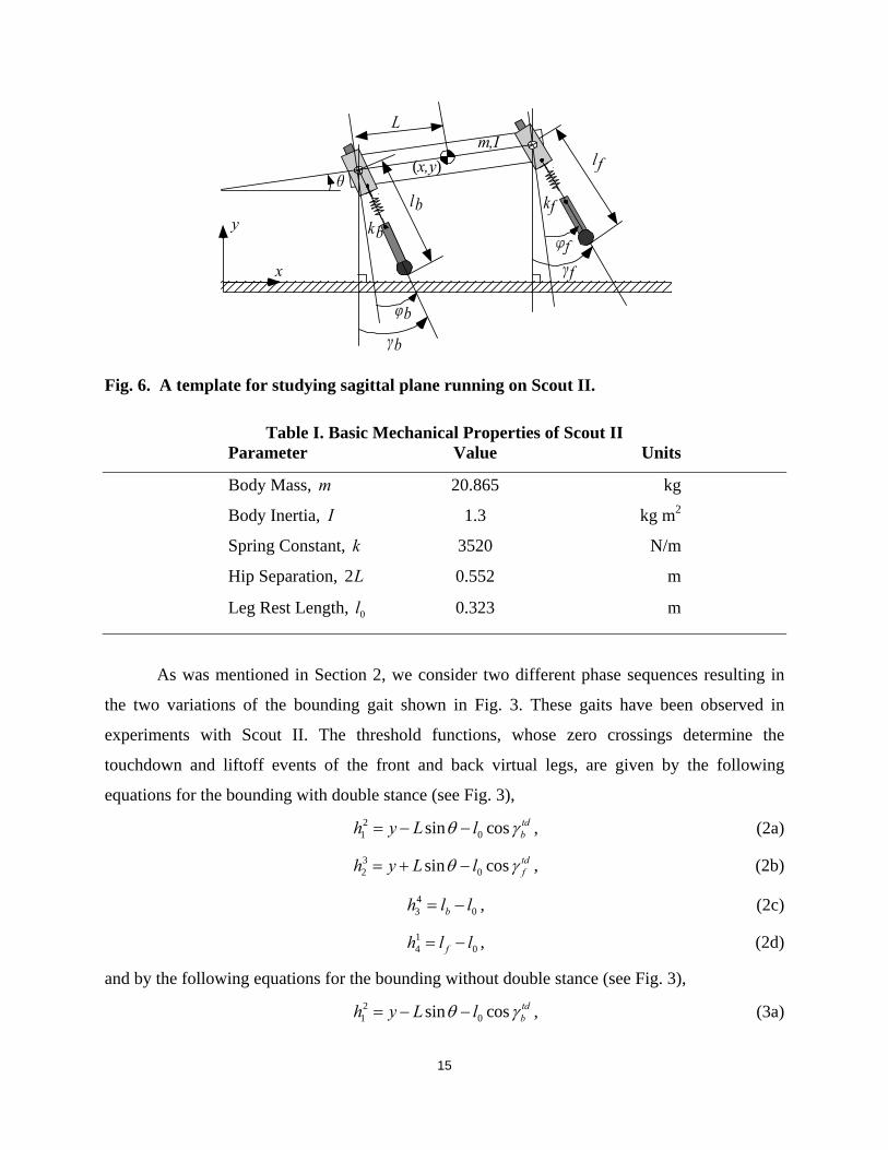
Fig. 6. A template for studying sagittal plane running on Scout II.

Table I. Basic Mechanical Properties of Scout II Parameter Value Units

Body Mass, m 20.865 kg

Body Inertia, I 1.3 kg m2

Spring Constant, k 3520 N/m

Hip Separation, 2 0.552 m L

Leg Rest Length, 0.323 m 0l

As was mentioned in Section 2, we consider two different phase sequences resulting in

the two variations of the bounding gait shown in Fig. 3. These gaits have been observed in

experiments with Scout II. The threshold functions, whose zero crossings determine the

touchdown and liftoff events of the front and back virtual legs, are given by the following

equations for the bounding with double stance (see Fig. 3),

21 0sin cos td

bh y L lθ γ= − − , (2a)

32 0sin cos td

fh y L lθ γ= + − , (2b)

43 bh l l0= − , (2c)

14 fh l l0= − , (2d)

and by the following equations for the bounding without double stance (see Fig. 3),

21 0sin cos td

bh y L lθ γ= − − , (3a)

15

16

0 12 bh l l= − , (3b)

31 0sin cos td

fh y L lθ γ= + − , (3c)

13 fh l l0= − , (3d)

where the superscript td denotes touchdown, the subscripts b and f denote the back and front

virtual legs respectively, and is the uncompressed leg length, see Table I. In (2) and (3),

zeroing of h

0l

βα corresponds to the event that signifies the transition from the flow describing

phase α to that describing phase β . All the other variables in (2) and (3) are defined in Fig. 6.

Note that in the second variation of the bounding phase sequence, the dynamics of the double

stance phase can be dropped in the calculation of the return map.

To define the return map, we first consider a convenient point in the bounding running

cycle. In this work we use the apex height in the double leg flight phase. We could select any

other point in the cycle. However, the selection of the apex height allows for the touchdown

angles of both the front and back virtual legs to explicitly appear in the definition of the return

map as kinematic inputs available for control. We define the Poincaré section, [17], to be the

hyperplane

{ }0ˆˆ ˆ | 0, sin cos , sin costd td

bX y y L l y L l0 fθ γ θΣ = ∈ = − > + >x & γ , (4)

where the conditions 0sin cos tdby L lθ γ− > and 0sin cos td

fy L lθ γ+ > were added to indicate that

the robot is in double leg flight ( becomes zero not only at the apex but also at the lowest

height). The system is at its apex when its orbit pierces the hyperplane

y&

Σ̂ . For the Poincaré map

to be properly defined it is necessary that Σ̂ satisfies the transversality condition (cf. [17]) i.e.

the inner product of the vector field and the hyperplane’s normal vector must never be zero. In

the coordinates ( , , , , , x y x y )θ θ&& & , the normal vector to the hyperplane is simply Σ̂

[ ]0 0 0 0 1 0 T=n . At apex the vector field is ( )1 apexˆ 0 0 0T

x gθ⎡ ⎤= −⎣ ⎦f x && , where

,x Rθ ∈&& , since when the system is in the double flight phase it follows a ballistic trajectory.

Hence, , i.e. the transversality condition is satisfied. ( )1 apexˆ 0T g= − ≠n f x

We seek a function that maps the apex height states of the th stride to those of the

) th stride. The states at the th apex height constitute the initial conditions for the cycle,

n

( 1n + n

17

based o

event

n which we integrate the double flight phase equations, until the back leg touchdown

occurs. This event triggers the back leg stance phase, whose dynamic equations are

integrated using as initial conditions the final conditions of the previous phase (since massless

legs are considered there are no impacts at touchdown). Successive forward integration of the

dynamic equations of all the phases, according to (2) and (3) for the two variations of the

bounding gait, yields the state vector x̂ at the ( )1n + th apex height, which is the value of the

Poincaré return map evaluated at the n th apex height. If the state vector at the new apex height is

identical to the initial the cycle is repetitive.

Note though that the state vector contains the horizontal coordinate x of the torso’s

COM, which is a monotonically increasing f x does not munc ime. Therefore, tion of t ap to itself

after a cycle, and a function that has been obtained by integrating (1) according to (2) and (3)

cannot have fixed points that correspond to the bounding gait. This issue can be resolved by

projecting out the horizontal component x of the state vector x̂ , which is not relevant to

describing the running gait. A further dimensional reduction can be obtained by noticing that on

the Poincaré section Σ̂ the variable y& is identically zero (this dime sional reduction is inherent

to the Poincaré method for stability, see

n

[17]). After the projection ˆ: X XΠ → ;

ˆT

y xθ θ⎡ ⎤=x x &a of the state vector ˆˆ X⎣ ⎦& ∈x onto its non x and y& components, the task

of studying passive bounding reduces to finding the fixed points of the return map

ion with independent coordinates 1 2X R S R

P acting on

the reduced Poincaré sect ∈ = × ×x i.e.

( )1 ,n n n+ =x P x u , (5)

with Ttd td

b fγ γ⎡ ⎤= ⎣ ⎦u , and the subscript n indicates the stride number.

Equation (5) represents a nonlinear discrete tim

do not participate in the

dynami

e system. As expected, despite the fact

that the touchdown angles are not part of the state vector and they

cs, they directly affect the value of the return map. The appearance of the touchdown

angles in the right hand side of (5) is a consequence of the dependence of the threshold functions

(2) and (3) on the touchdown angles’ values. It is apparent from (5) that the touchdown angles

are kinematic inputs available for “cheap” control, since, in Scout II, it is very easy to place the

legs at their target angles during the flight phase. The significance of the flight phase in the

control of running has also been outlined in [3], where it was shown that, in the passive and

conservative SLIP, the stance phase has no contribution to the stability of the gait, while

different leg placement strategies during flight result in different stability properties.

5 EXISTENCE OF PASSIVE BOUNDING CYCLES

5.1 Fixed Points and their Properties

18

o determine the conditions required to permit steady

state cyclic bounding motion of Scout II. In other words we want to find an argument in (5)

The goal of the analysis in this section is t

x

that maps onto itself, i.e. we want to solve the equation

( ),− =x P x u 0 , (6)

for all (experimentally) reasonable values of touchdown angles . Existence of solutions for (6)

not guaranteed, but seems to be the rule rather than th

e

mplexity of the equations

preclud

u

is e exception.

The search space is 4-dimensional with two free paramet rs, since for different values of

touchdown angles, different solutions may be obtained. The co

es describing P as a nonlinear function by analytically integrating the dynamics.

Therefore, we resort to numerical evaluation of the return map, and use a Newton-Raphson

method for finding its fixed points. Thus, an initial guess 0nx for the fixed point is assumed and

then updated using the equation

( )( ) ( )11k k k k

n n

−+ k

n n n⎡ ⎤= + −∇ −⎣ ⎦x

where corresponds to the apex height, corresponds to the number of iterations, and the

radient matrix (Jacobian) of the return map is given by

x x I P x P x , (7)

thn n k

g

y xθ θ

⎡ ⎤∂ ∂ ∂ ∂ ∂=∇ = ⎢ ⎥∂ ∂ ∂ ∂ ∂⎣ ⎦&&

To find a solution, we evaluate (7) iteratively un

P P P P PPx

. (8)

til convergence (the error

). The value of at P knx1 510k k

n n+ −

∞− <x x is calculated through the numerical integration of the

dynami

was used in MAT

c equations during a complete cycle. To do that, the adaptive step Dormand-Price method

LAB™ with 1 10e and 1 9e− − relative and absolute tolerances, respectively.

To evaluate numerically the Jacobian of the return map, the related partial derivatives are

approximated using central differences. Each iteration involves nine evaluations of the return

map P : One corresponds to calculating P at the nominal point knx , and eight to calculate the

gradients. More specifically to compute the components ix∂ ∂P , 1, , 4i = K , of the gradient

matrix ∇P , we need four evaluations of at P kn d−x x (fore of the nominal point), and four at

k

x by some small scalar quantity

n (aft of the nominal point), where is obtained by perturb each of components of d+x x dx ing

ε (in im e we used 1 6eplementing this schem ε = − ).

g (7) is computationally intensive owever, if the initial guess is reasonableEvalua ; h

so

some v

tin 7 and a

lution exists, this method finds it usu lly in less than eleven iterations.

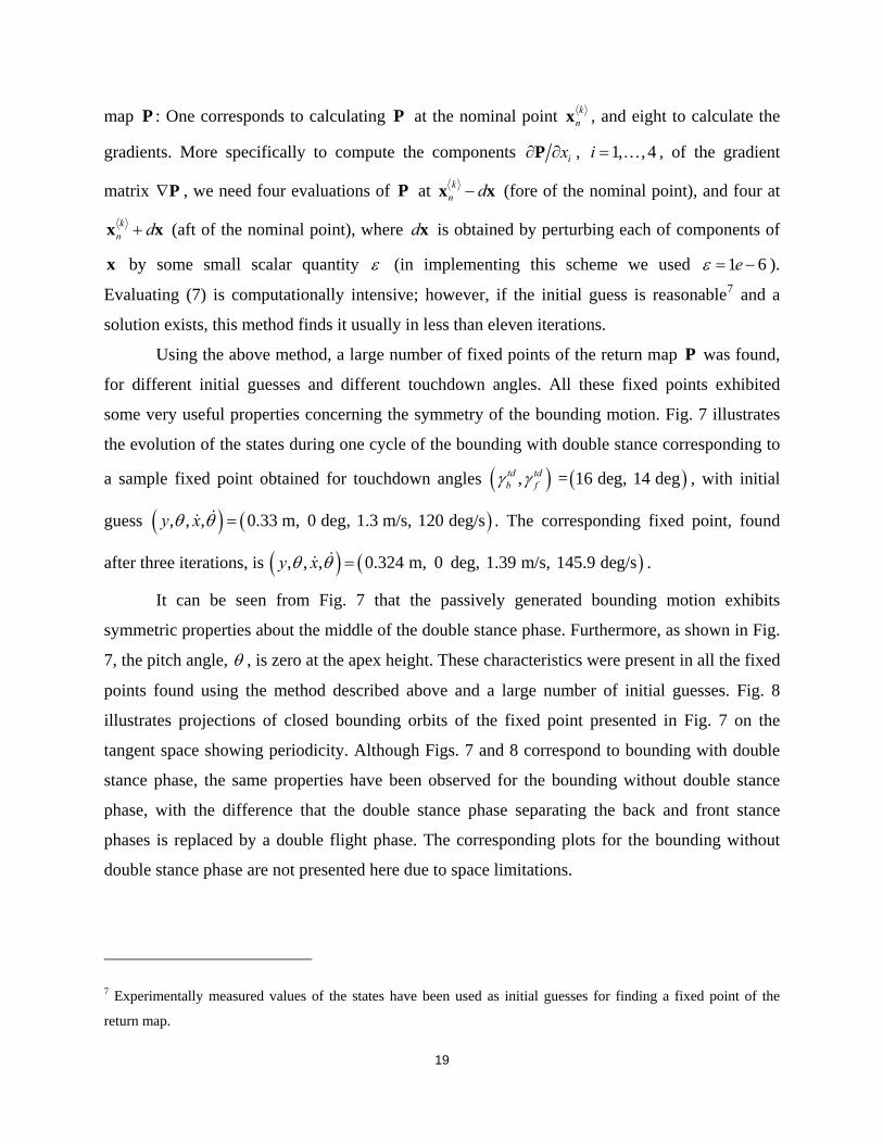
Using the above method, a large number of fixed points of the return map P was found,

for different initial guesses and different touchdown angles. All these

a

fixed points exhibited

ery useful properties concerning the symmetry of the bounding motion. Fig. 7 illustrates

the evolution of the states during one cycle of the bounding with double stance corresponding to

a sample fixed point obtained for touchdown angles ( ) ( ), = 16 deg, 14 degtd tdb fγ γ , with initial

( )guess ( )&

after three iterations, is

, , , 0.33 m, 0 deg, 1.3 m/s, 120 deg/sy xθ θ =& . The corresponding fixed point, found

( ) ( ), , , 0.324 m, 0 deg, 1.39 m/s, 145.9 deg/sy xθ θ =&& .

It can be seen from Fig. 7 that the passively generated bounding motion exhibits

out the middle of the double stance phase. Furthermore, as shown in Fig.

7, the p

symmetric properties ab

itch angle, θ , is zero at the apex height. These characteristics were present in all the fixed

points found using the method described above and a large number of initial guesses. Fig. 8

illustrates projections of closed bounding orbits of the fixed point presented in Fig. 7 on the

tangent space showing periodicity. Although Figs. 7 and 8 correspond to bounding with double

stance phase, the same properties have been observed for the bounding without double stance

phase, with the difference that the double stance phase separating the back and front stance

phases is replaced by a double flight phase. The corresponding plots for the bounding without

double stance phase are not presented here due to space limitations.

7 Experimentally measured values of the states have been used as initial guesses for finding a fixed point of the

return map.

19

Fig. 7. Evolution of the states at bounding with double stance during one cycle. The

vertical lines show the events: Back leg touchdown, front leg touchdown, back leg liftoff,

and front leg liftoff.

Fig. 8. Projections of bounding orbits on the tangent space for the fixed point shown in Fig.

7 (bounding with double leg stance).

Fig. 9 presents the leg lengths and the leg angles for the back and front virtual legs during

one cycle and for the fixed point of Fig. 7. Careful inspection of Fig. 9 reveals another important

property of the fixed points. It can be seen that the touchdown angle of the front leg is equal to

20

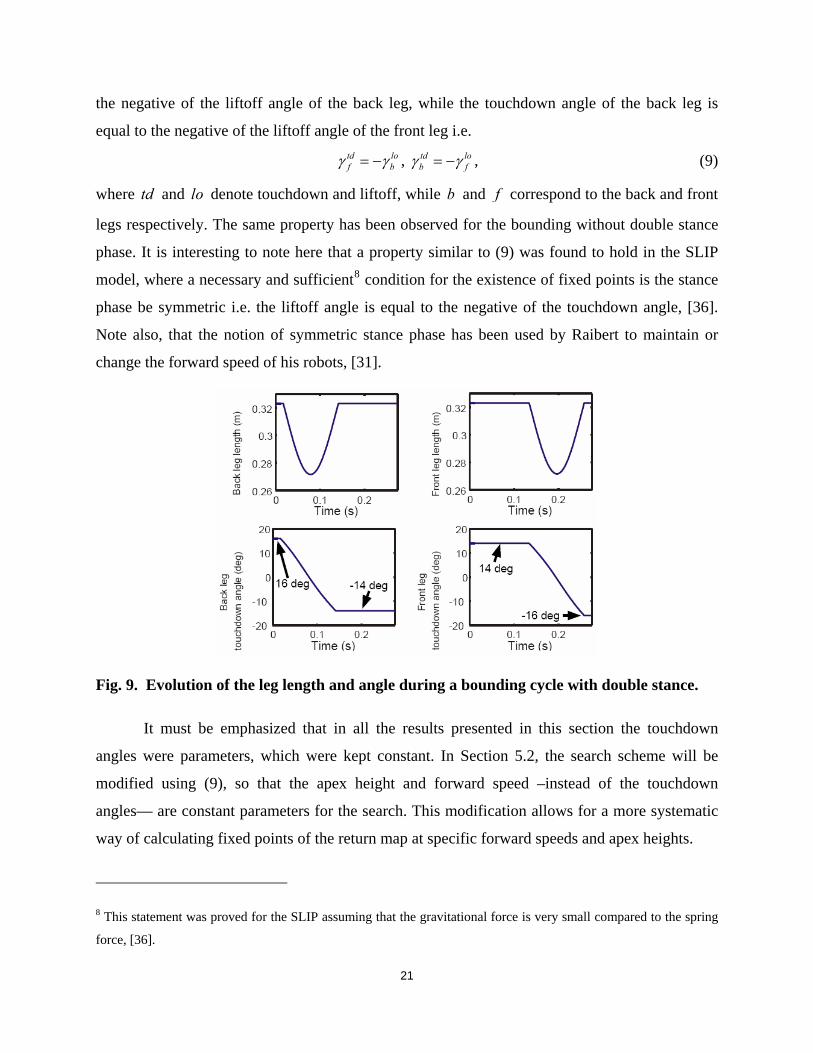
the negative of the liftoff angle of the back leg, while the touchdown angle of the back leg is

equal to the negative of the liftoff angle of the front leg i.e.

td lof bγ γ= − , td lo

b fγ γ= − , (9)

where td and lo denote touchdown and liftoff, while b and f correspond to the back and front

legs respectively. The same property has been observed for the bounding without double stance

phase. It is interesting to note here that a property similar to (9) was found to hold in the SLIP

model, where a necessary and sufficient8 condition for the existence of fixed points is the stance

phase be symmetric i.e. the liftoff angle is equal to the negative of the touchdown angle, [36].

Note also, that the notion of symmetric stance phase has been used by Raibert to maintain or

change the forward speed of his robots, [31].

Fig. 9. Evolution of the leg length and angle during a bounding cycle with double stance.

It must be emphasized that in all the results presented in this section the touchdown

angles were parameters, which were kept constant. In Section 5.2, the search scheme will be

modified using (9), so that the apex height and forward speed –instead of the touchdown

angles— are constant parameters for the search. This modification allows for a more systematic

way of calculating fixed points of the return map at specific forward speeds and apex heights.

8 This statement was proved for the SLIP assuming that the gravitational force is very small compared to the spring

force, [36].

21

5.2 Continuums of Symmetric Fixed Points

For Scout II's bounding running, a specific horizontal speed and a sufficient apex height that

prevents toe stubbing are useful functional requirements. Therefore, the search scheme described

above is modified in this section, so that the forward speed and apex height become its input

parameters, specified according to running requirements and kept constant during the search. The

touchdown angles are now considered to be “states” of the searching procedure, i.e. variables to

be determined from it. By doing so, the search space states and the vector of the parameters

(“inputs” to the search scheme) are respectively

, * Ttd tdb fθ θ γ γ⎡ ⎤= ⎣ ⎦x & [ ]* Ty x=u & , (10)

and the return map whose fixed points are to be calculated becomes ( )* * *

1 ,n n+ =x P x u*n . (11)

It is important to mention that the numerical integration of the equations of motion starting from

the apex height event, results in the calculation of the liftoff angles ( )lob nγ , and not of the

touchdown angles of the legs at the next apex height event. This is a consequence of the

assumption of massless legs. Thus, to calculate the gradients needed to implement the Newton-

Raphson scheme, the liftoff angles must be “mapped” to touchdown angles based on the

symmetry described by (9) i.e.

( )lof n

γ

( ) ( )1

td lob fn nγ γ

+= − and ( ) ( )

1

td lof n

γ+= − b n

γ . (12)

Then, by using the Newton-Raphson algorithm, we update the initial guess until convergence is

achieved.

The above search scheme does not explicitly ensure that the following conditions are

satisfied,

1n ny y+ = , 1n nx x+ =& & , (13)

which are a direct consequence of the definition of a fixed point. Instead, in the new search

scheme, we required that (12) holds. However, examination of the search results shows that,

provided that (12) holds, (13) also holds. Note that this behavior is analogous to that of the SLIP,

where the symmetric stance phase is a condition for a fixed point, [36].

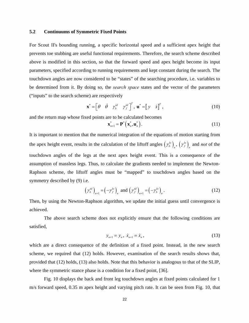
Fig. 10 displays the back and front leg touchdown angles at fixed points calculated for 1

m/s forward speed, 0.35 m apex height and varying pitch rate. It can be seen from Fig. 10, that

22

there exists a continuum of fixed points, which lie on two inner branches, accompanied by two

outer branches. Fixed points lying in the shadow area correspond to the bounding gait with a

double stance phase, while fixed points outside this area correspond to the bounding without a

double stance phase (cf. Fig. 3). It is interesting to note that for both the inner and outer

branches, and for some given forward speed and apex height, the system shows preference

towards the bounding with double stance for low pitch rates. As the pitch rate, and thus the

energy content of the system, increases, the duration of the double stance phase continuously

decreases, until a point where it becomes zero. This point signifies the transition from the

bounding with a double stance phase to the bounding without; no overlapping between the two

variations of the bounding gait is present. It is important to mention that the same tendency has

also been observed experimentally with Scout II. For lower system energies the robot converges

to a bounding motion with a double stance phase. This fact indicates a qualitative agreement

between experiments and the results of Fig. 10.

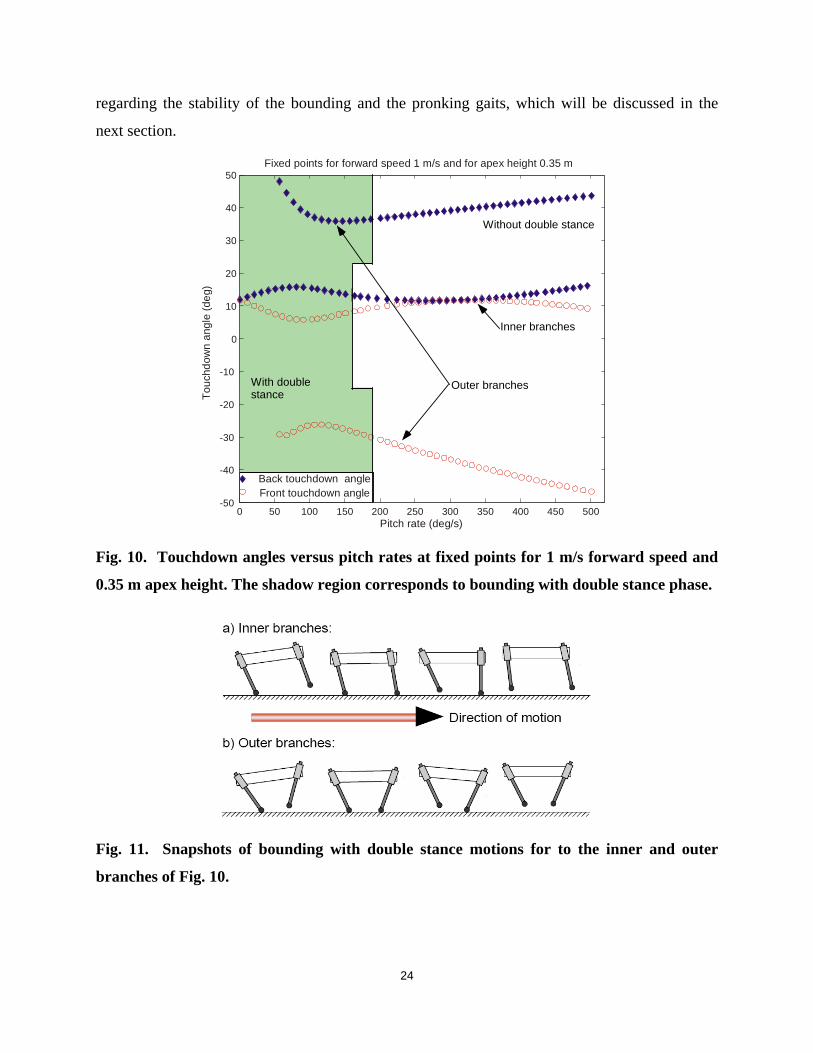
Furthermore, the existence of the outer branches in Fig. 10 shows that there is a range of

pitch rates where two different fixed points exist for the same forward speed, apex height and

pitch rate. This is quite surprising, since the same total energy and the same distribution of that

energy among the three modes of the motion –forward, vertical and pitch— results in two

different motions depending on the touchdown angles. As can be seen from Fig. 11, the fixed

points that lie on the inner branch correspond to a bounding motion similar to the one observed

in experiments with Scout II: the front leg is brought in front of the torso. However, the fixed

points that lie on the outer branch correspond to a motion where the front leg is brought towards

the torso’s COM. The pattern of Fig. 11 b) resembles the dynamic walking gait implemented on

Scout II, see [12], which is only present at lower speeds.

In reading Fig. 10, it is useful to note that the region close to the vertical axis corresponds

to pronking-like motions. Indeed, recall that, at the apex height the pitch angle is zero ( 0θ = )

always, (see Fig. 7 in Section 5.1). As we approach the vertical axis of Fig. 10 ( 0θ =& ), the

touchdown angles of the front and back legs tend to become equal. A gait with 0θ = , 0θ =& and

equal touchdown angles for the front and back legs corresponds to the pronking gait, where the

front and back legs strike and leave the ground in unison. Therefore, points near the vertical axis

correspond to pronking-like motions. This observation will lead to some useful conclusions

23

regarding the stability of the bounding and the pronking gaits, which will be discussed in the

next section.

Back touchdown angleFront touchdown angle

0 50 100 150 200 250 300 350 400 450 500-50

-40

-30

-20

-10

0

10

20

30

40

50

Pitch rate (deg/s)

Touc

hdow

nan

gle

(deg

)

Fixed points for forward speed 1 m/s and for apex height 0.35 m

Without double stance

With doublestance

Inner branches

Outer branches

Fig. 10. Touchdown angles versus pitch rates at fixed points for 1 m/s forward speed and

0.35 m apex height. The shadow region corresponds to bounding with double stance phase.

Fig. 11. Snapshots of bounding with double stance motions for to the inner and outer

branches of Fig. 10.

24

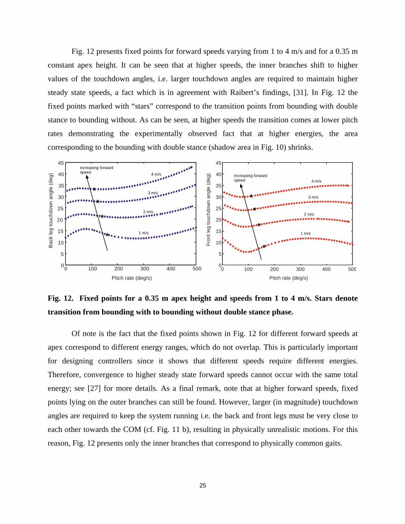
Fig. 12 presents fixed points for forward speeds varying from 1 to 4 m/s and for a 0.35 m

constant apex height. It can be seen that at higher speeds, the inner branches shift to higher

values of the touchdown angles, i.e. larger touchdown angles are required to maintain higher

steady state speeds, a fact which is in agreement with Raibert’s findings, [31]. In Fig. 12 the

fixed points marked with “stars” correspond to the transition points from bounding with double

stance to bounding without. As can be seen, at higher speeds the transition comes at lower pitch

rates demonstrating the experimentally observed fact that at higher energies, the area

corresponding to the bounding with double stance (shadow area in Fig. 10) shrinks.

0 100 200 300 400 5000

5

10

15

20

25

30

35

40

45

Pitch rate (deg/s)

Bac

kle

gto

uchd

own

angl

e(d

eg)

increasing forwardspeed

1 m/s

2 m/s

3 m/s

4 m/s

0 100 200 300 400 500

0

5

10

15

20

25

30

35

40

45

Pitch rate (deg/s)

Fron

tleg

touc

hdow

nan

gle

(deg

) increasing forwardspeed

1 m/s

2 m/s

3 m/s

4 m/s

Fig. 12. Fixed points for a 0.35 m apex height and speeds from 1 to 4 m/s. Stars denote

transition from bounding with to bounding without double stance phase.

Of note is the fact that the fixed points shown in Fig. 12 for different forward speeds at

apex correspond to different energy ranges, which do not overlap. This is particularly important

for designing controllers since it shows that different speeds require different energies.

Therefore, convergence to higher steady state forward speeds cannot occur with the same total

energy; see [27] for more details. As a final remark, note that at higher forward speeds, fixed

points lying on the outer branches can still be found. However, larger (in magnitude) touchdown

angles are required to keep the system running i.e. the back and front legs must be very close to

each other towards the COM (cf. Fig. 11 b), resulting in physically unrealistic motions. For this

reason, Fig. 12 presents only the inner branches that correspond to physically common gaits.

25

6 LOCAL STABILITY OF PASSIVE BOUNDING

The existence of passively generated bounding running cycles is by itself a very important result,

since it shows that an activity as complex as bounding running can simply be a natural motion of

the system. However, in real situations the robot is continuously perturbed, therefore, if a fixed

point were unstable, then the periodic motion would not be sustainable without control effort. In

this section we characterize the stability of the fixed points found in Section 5.

To investigate stability, we assume that the apex height states are perturbed from their

nominal values ( , )x u , by some small amount ( , )Δ Δx u . The discrete model that relates the

deviations from steady state is

1n n+ nΔ = Δ + Δx A x B u , (14)

where Δ = −x x x , Δ = −u u u and

( ),= ∂ ∂ x=xu=u

A P x u x , ( ),= ∂ ∂ x=xu=u

B P x u u .

For small perturbations, the apex height states at the next stride can be calculated by the linear

difference equations (14). If all the eigenvalues of the system matrix have magnitude less

than one, then the periodic solution is stable.

A

Fig. 13 shows the loci of the eigenvalues of matrix for the bounding with and without

double stance phase and for both the inner and outer branches of the fixed points presented in

Fig. 10, as the pitch rate varies. In reading Fig. 13 note that the encircled numbers show the

initial locations of the eigenvalues, which, as the pitch rate increases, move along the directions

of the arrows, on the root locus, and converge to the points marked by “x”. As was expected, in

all cases, one of the eigenvalues is located at one, representing the fact that the system is

conservative

A

9 (for the sake of clarity the point at which eigenvalue 1 converges is not marked by

“x” since it remains always at one). Fig. 13 (a) corresponds to the inner branch of the bounding

with double stance phase (cf. Fig. 10). Two of the eigenvalues, namely 2 and 3, start on the real

axis, and as θ& increases they move towards each other, they meet on the real axis, and finally

they move towards the rim of the unit circle. The third eigenvalue, marked by 4, starts at a high

9 The conservative nature of the system could have been used to further reduce the dimension of the Poincaré return

map in (5). However, we have decided to keep this extra dimension for reasons of verification.

26

value and moves towards the unit circle, but it never gets into it, for those specific values of

forward speed and apex height. The situation is similar for the outer branch of the bounding with

double stance phase, as shown in Fig. 13 (c). Figs. 13 (b) and (d) illustrate the loci of the

eigenvalues for the inner and outer branches of the bounding without a double stance phase.

Again eigenvalue 1 is located at one. Eigenvalues 2 and 3 start at the points where they stopped

during the bounding with double stance phase as shown in Figs. 13 (a) and (c). In Fig. 13 (b)

they move close to the rim of the unit circle, but always stay outside of it. In Fig. 13 (d) they

move in arcs further away from the unit circle until they meet each other on the real axis, after

which they move in opposite directions. Eigenvalue 4 starts from the location at which it stopped

in the bounding with double stance phase, and in Fig. 13 (b) it moves on the real axis away from

the unit circle, while in Fig. 13 (d) it moves towards the unit circle.

Fig. 13. Root locus showing the paths of the four eigenvalues as the pitch rate increases for

the inner (up) and the outer (down) branches of fixed points. The numbers show the

starting points of the eigenvalues, “x” denotes the points where the eigenvalues converge,

and the arrows show the direction of their motion.

In all the above cases there is always at least one eigenvalue outside of the unit circle at

every value of the pitch rate. Therefore, there is no region of parameters where the system is

27

passively stable for forward speed 1 m/sx =& and apex height 0.35 my = . Note that similar, but

not identical, root loci as those presented in Fig. 13 are observed at different forward speeds and

apex heights, the difference being the values the eigenvalues attain as the pitch rate increases.

To show how the forward speed affects the stability of the motion, we present Fig. 14,

which shows the magnitude of the larger eigenvalue at different forward speeds for the inner

branches of the bounding with and without double stance phase. In this figure, the stars denote

transition from bounding with a double stance phase to bounding without one. For sufficiently

high forward speeds and for a region of pitch rates, the larger eigenvalue enters the unit circle,

while the other two eigenvalues remain well behaved. This fact shows that, for these parameter

values, the system is self-stabilized. Furthermore, it is apparent from Fig. 14 that the self-

stabilization regime is present in both variations of the bounding gait, i.e. with and without

double stance phase. It is worth mentioning here that, as depicted in Fig. 14, the largest

eigenvalue obtains its maximum value when the pitch rate θ& is small. Recall that the region

where θ& takes small values corresponds to a pronking-like motion, where both the front and

back legs hit and leave the ground in unison. Thus, we can conclude that pronking-like motions

(low-pitch rates) are “more unstable” than bounding, (high pitch rates). This fact was also

observed in experiments with Scout II.

Fig. 14. Largest eigenvalue norm at various pitch rates and for forward speeds 1 to 4 m/s.

The stars denote transition from bounding with to bounding without double stance.

28

The details of the root locus are shown in Fig. 15. The shape of the root locus is similar to

the root loci presented in Fig. 13 (a) and (b), except for the fact that, for some values of the pitch

rate, eigenvalues 2, 3 and 4 are all inside the unit circle. Note that the changes in the slope of the

norm of the larger eigenvalue in Fig. 14 are attributed to the fact that, as the eigenvalues move

along the branches of the root locus, the eigenvalue that has the larger norm changes; see Fig. 15.

Fig. 15. Root loci for the inner branches of the bounding with (up) and without (down)

double stance and for forward speed 4 m/s. The apex height is 0.35 m.

Interestingly, despite the apparent simplicity of the quadrupedal model presented above,

compared to the complexity of more accurate models of Scout II, as those described in [29], we

have been able to reproduce, qualitatively, many different behaviors, which have also been

observed experimentally on the robot. These behaviors include both variations of bounding

described in Fig. 3, and also pronking-like and dynamic walking motions. Furthermore, a good

qualitative agreement between the bounding results presented in this paper and the experimental

data of [29] has been observed. For instance, the pitch angle as shown in Fig. 7 bears remarkable

resemblance to the corresponding one measured in experiments (see Fig. 12 in [29]). Moreover,

self-stabilization occurs in a range of pitch rates, which is in agreement with the pitch rates

measured in experiments with Scout II. However, experimental Scout II runs are stable at

approximately 1/3 the speeds predicted here. This is most probably due to the stance-brake phase

29

30

present in the controller in experiments; see Fig. 2. The stance-brake phase results in decelerating

the robot, and breaks the touchdown-liftoff symmetry presented in Fig. 9. As is described in

detail in [29], it also results in errors between simulation results and experimental data, even in

more accurate models of Scout II. However, including the stance-brake phase in the controller is

necessary for ensuring toe clearance, especially during the early protraction phase, due to the

absence of active control of the leg length during flight.

Furthermore, effects not present in passive models, such as actuator dynamics, damping

in the leg prismatic joints, intermittent stick/slip of the foot-ground contact, and energy losses at

touchdown due to impact, may contribute to discrepancies between the conservative model

studied here and the robot, such as the difference in the forward speed. More specifically,

regarding the role of the actuators during stance, it is noted that large peaks in the torques appear

at the early phases of the stance-retraction phase. However, as is explained in detail in [29] (see

Figs. 14 and 15 in [29]), motor saturation comes almost immediately after touchdown, resulting

in very small torques throughout the stance-retraction phase, until the stance-brake phase is

reached. The exact role of the actuator dynamics in the resulting motion is currently under

investigation.

The main conclusion from the analysis above is that there exists a regime where the

system can be passively stable. This is an important result since it shows that the system can

tolerate small perturbations away from the nominal conditions without any control action taken.

This fact could provide a possible explanation to why Scout II can bound without the need of

complex state feedback, using very simple control laws that only excite its natural dynamics, and

is in agreement with recent research from biomechanics, which shows that, when animals run at

high speeds, passive dynamic self-stabilization from a feedforward, tuned mechanical system can

reject rapid perturbations and simplify control [14], [21]. Analogous behavior has been

discovered by McGeer in his passive bipedal running work, [22], and recently in the SLIP

template, [15], [37].

7 CONCLUSION

In this paper, we studied the passive dynamics of the bounding running gait of a simple passive

and conservative model of our Scout II robot. Based on the analysis of numerically derived

return maps, we found that the two variations of the bounding gait, which have been

31

experimentally observed on Scout II, can be passively generated with appropriate initial

conditions. Most strikingly, in both bounding variations, there exists a regime where the model

stabilizes itself without the need of any control action! This is the first time that more elaborate

gaits, such as Scout II’s bounding, are found to be inherently stable, and is in agreement with

recent results from biomechanics, contributing to the increasing evidence that simple controllers,

as those reported in [29] that operate mostly in the feedforward regime, are adequate in

stabilizing a complex dynamic task like quadrupedal bounding. Most importantly, self-

stabilization can facilitate the design of more robust, yet minimalistic, controllers for

dynamically stable legged locomotion, by deriving control laws that expand the domain of

attraction of the self-stable behavior. A simplified model, such as the one presented in this paper,

that captures the essentials of the motion, can form the basis of a controlled model in a way

similar to that presented in [1] and [2], resulting in high performance combined with great energy

efficiency. Proposing such a controller for quadrupeds, and implementing it experimentally on

Scout II is our goal. The model presented in this paper provides the first step towards this goal.

ACKNOWLEDGMENTS

Support by the Institute of Robotics and Intelligent Systems (IRIS III, a Canadian Federal

Network of Centres of Excellence), and by the Natural Sciences and Engineering Research

Council of Canada (NSERC) is gratefully acknowledged. The second author would like to

acknowledge support by a PENED 2003 Grant by the Hellenic General Research and

Technology Secretariat. The work of I. Poulakakis has been supported by a R. Tomlinson

Doctoral Fellowship Award and by the Greville Smith McGill Major Scholarship while at

McGill University, and by the W. Benton Fellowship at The University of Michigan.

REFERENCES

[1] Ahmadi M., and Buehler M., “Stable Control of a Simulated Running Robot with Hip

and Leg Compliance”, IEEE Tr. on Robotics and Automation, Vol. 13, No. 1, pp. 96-104,

1997.

32

[2] Ahmadi M., and Buehler M., “The ARL Monopod II Running Robot: Control and

Energetics”, Proc. of IEEE Int. Conf. on Robotics and Automation, pp. 1689-1694,

Detroit, USA, 1999.

[3] Altendorfer R., Koditschek D. E., and Holmes P., “Stability Analysis of Legged

Locomotion by Symmetry-Factored Maps”, The Int. J. of Robotics Research, Vol. 23, No

10-11, pp. 979-1000, 2004.

[4] Berkemeier M. D., “Modeling the Dynamics of Quadrupedal Running”, The Int. J. of

Robotics Research, Vol. 17, No 9, pp. 971-985, 1998.

[5] Berns K. “Walking Machine Catalogue”, http://www.walking-machines.org/ (last

accessed March 14, 2006).

[6] Brown Jr. H. B., “Analysis of Planar Model for Two Limiting Cases”, Technical Report,

CMU-LL-4-1985, Carnegie Mellon University, The Robotics Institute, Pittsburgh, PA,

USA, February 1985.

[7] Buehler M., “Dynamic Locomotion with One, Four and Six-Legged Robots”, J. of the

Robotics Society of Japan, Vol. 20, No. 3, pp. 15-20, 2002.

[8] Campbell D. and Buehler M., “Preliminary Bounding Experiments in a Dynamic

Hexapod,” B. Siciliano and P. Dario (Eds.), Experimental Robotics VIII, pp. 612-621,

Springer-Verlag, 2003.

[9] Cham J. G., Bailey S. A. and Cutkosky M. R., “Robust Dynamic Locomotion through

Feedforward - Preflex Interaction”, ASME Int. Mechanical Engineers Congress and

Exposition (IMECE), Orlando FL, 2000.

[10] Cham J. G., Bailey S. A., Clark J. E., Full R. J., and Cutkosky M. R., “Fast and Robust:

Hexapedal Robots via Shape Deposition Manufacturing”, The Int. J. of Robotics

Research, Vol. 21, No. 10, pp. 869-882, 2002.

[11] Cherouvim N., and Papadopoulos E., “Single Actuator Control Analysis of a Planar

3DOF Hopping Robot”, S. Thrun, G. Sukhatme, S. Schaal (Eds.), Robotics: Science and

Systems I, pp. 145-152, MIT Press, Cambridge MA, 2005.

33

[12] de Lasa M. and Buehler M., “Dynamic Compliant Walking”, Proc. of IEEE Int. Conf. on

Robotics and Automation, Vol. 3. pp. 3153-3158, Seoul, Korea, 2001.

[13] Fukuoka Y., Kimura H., and Cohen A., “Adaptive Dynamic Walking of a Quadruped

Robot on Irregular Terrain Based on Biological Concepts”, The Int. J. of Robotics

Research, Vol. 22, No. 3-4, pp. 187-202, 2003.

[14] Full R. J. and Koditschek D., “Templates and Anchors: Neuromechanical Hypotheses of

Legged Locomotion on Land”, J. of Experimental Biology, 202, pp. 3325-3332, 1999.

[15] Ghigliazza R. M., Altendorfer R., Holmes P. and Koditschek D. E., “A Simply Stabilized

Running Model”, SIAM J. of Applied Dynamical Systems, Vol. 2, No. 2, pp. 187-218,

2003.

[16] Grizzle J. W., Abba G., and Plestan F., “Asymptotically Stable Walking for Biped

Robots: Analysis via Systems with Impulse Effects”, IEEE Tr. on Aut. Control, Vol. 46,

No. 1, pp. 51-64, 2001.

[17] Guckenheimer J. and Holmes P., Nonlinear Oscillations, Dynamical Systems, and

Bifurcations of Vector Fields, Applied Mathematical Sciences, Vol. 42, Springer-Verlag,

NY, 1983.

[18] Guckenheimer J. and Johnson S., “Planar Hybrid Systems”, in Hybrid Systems II, Lect.

Notes in Comp. Science, pp 202-225, Springer-Verlag, 1995.

[19] Iida F. and Pfeifer R., “Cheap Rapid Locomotion of a Quadruped Robot: Self-

Stabilization of Bounding Gait”, Intelligent Autonomous Systems 8, F. Groen et al. (Eds.),

pp. 642-649, IOS Press: Amsterdam, The Netherlands, 2004.

[20] Kimura H., Akiyama S. and Sakurama K., “Realization of Dynamic Walking and

Running of the Quadruped Using Neural Oscillator,” Proc. of the IEEE/RSJ Int. Conf. on

Intelligent Robots and Systems, pp. 406 – 412, Victoria, Canada, 1998.

[21] Kubow T. and Full R., “The Role of the Mechanical System in Control: A Hypothesis of

Self-stabilization in Hexapedal Runners,” Phil. Trans. of the Royal Society of London

Series B – Biological Sciences, 354 (1385), pp. 854-862, 1999.

34

[22] McGeer T., “Passive Bipedal Running”, Technical Report, CSS–IS TR 89-02, Simon

Fraser University, Centre For Systems Science, Burnaby, BC, Canada, 1989.

[23] McGeer T., “Passive Dynamic Walking”, The Int. J. of Robotics Research, Vol. 9, No. 2,

pp. 62 – 82, 1990.

[24] McMahon T., Muscles, Reflexes, and Locomotion, Princeton University Press, 1985.

[25] Murphy K. N., “Trotting and Bounding in a Simple Planar Model”, Technical Report,

CMU-LL-4-1985, Carnegie Mellon University, The Robotics Institute, Pittsburgh, PA,

USA, February 1985.

[26] Pearson K., “The Control of Walking”, Scientific American, Vol. 72, p. 86, 1976.

[27] Poulakakis I., On the Passive Dynamics of Quadrupedal Running, M. Eng. Thesis,

McGill University, Montreal, QC, Canada, July 2002.

[28] Poulakakis I., Papadopoulos E. and Buehler M., “On the Stable Passive Dynamics of

Quadrupedal Running”, Proc. of the IEEE Int. Conf. on Robotics and Automation, pp.

1368-1373, Taipei, Taiwan, 2003.

[29] Poulakakis I., Smith J. A., and Buehler M., “Modeling and Experiments of Untethered

Quadrupedal Running with a Bounding Gait: The Scout II Robot”, The Int. J. of Robotic

Research, Vol. 24, No. 4, pp. 239-256, 2005.

[30] Poulakakis I., Smith J. A., and Buehler M., “On the Dynamics of Bounding and

Extensions Towards the Half-Bound and the Gallop Gaits”, H. Kimura, K. Tsuchiya, A.

Ishiguro, and H. Witte (Eds.), Adaptive Motion of Animals and Machines, pp. 79-88,

Springer-Verlag, 2005.

[31] Raibert M. H., Legged Robots that Balance, MIT Press, Cambridge MA, 1986.

[32] Saranli U., Buehler M., and Koditschek D. E., “RHex: A Simple and Highly Mobile

Hexapod Robot”, The Int. J. Robotics Research, Vol. 20, No. 7, pp. 616-631, 2001.

[33] Saranli U., and Koditschek D. E., “Template Based Control of Hexapedal Running”,

Proc. of the IEEE Int. Conf. on Robotics and Automation, Vol. 1, pp. 1374-1379, Taipei,

Taiwan, 2003.

35

[34] Scheck F., Mechanics: From Newton Laws to Deterministic Chaos, Third Ed., Springer-

Verlag, Berlin, 1999.

[35] Schmitt J. and Holmes P., “Mechanical models for insect Locomotion: Dynamics and

Stability in the Horizontal Plane I. Theory”, Biological Cybernetics, Vol. 83, pp. 501 –

515, 2000.

[36] Schwind W., Spring Loaded Inverted Pendulum Running: A Plant Model, PhD Thesis,

The University of Michigan, Ann Arbor, MI, U.S.A., 1998.

[37] Seyfarth A., Geyer H., Guenther M. and Blickhan R., “A Movement Criterion for

Running”, J. of Biomechanics, Vol. 35, pp. 649-655, 2002.

[38] Smith J. A. and Poulakakis I., “Rotary Gallop in the Untethered Quadrupedal Robot

Scout II”, Proc. of the IEEE/RSJ Int. Conf. on Intelligent Robots and Systems, pp. 406 –

412, Sendai, Japan, 2004.

[39] Weingarten J. D., Lopes G. A. D., Buehler M., Groff R. E., and Koditschek D. E.,

“Automated Gait Adaptation for Legged Robots”, Proc. of the IEEE Int. Conf. on

Robotics and Automation, Vol. 3, pp. 2153-2158, New Orleans, USA, 2004.

[40] Yamamoto Y., Fujita M., De Lasa M., Talebi S., Jewell D., Playter R. and Raibert M.,

“Development of Dynamic Locomotion for the Entertainment Robot – Teaching a New

Dog Old Tricks, 4th Int. Conf. on Climbing and Walking Robots, pp. 695 - 702, 2001.

[41] Zhang Z. G., Fukuoka Y. and Kimura H., “Stable Quadrupedal Running based on a

Spring-Loaded Two-Segment Legged Model”, Proc. of the IEEE Int. Conf. on Robotics

and Automation, Vol. 3, pp. 2601-2606, New Orleans, USA, 2004.