2/4/2009 DRAFT

1

Quadrature (Complex-Valued) Signal Processing

A Technical Overview Jim Shima

Quadrature Signals Redux

Quadrature, or complex-valued, signals refer to waveforms that are deemed “analytic”. In

this context, an analytic signal is one which has a frequency response containing only

positive frequency terms. In this paper, the terms “quadrature” and “analytic” are

sometimes used interchangeably.

Recall from Fourier theory, all real-valued signals have “symmetric” positive and negative

frequency terms. For analytic signals, the negative portion of the frequency response

disappears. Analytic signals are also related to Hilbert transforms, as they can be

represented by:

{ })()()( txHjtxtxquad ⋅+= (1.1)

Where H{x(t)}is the Hilbert transform of the real signal x(t). By definition, the Hilbert

transform shifts the input signal 90 degrees for negative frequencies, and -90 degrees for

positive frequencies [2]. If x(t) is a sinusoid, you can easily see that the Hilbert transform

turns sines into cosines, and vice versa. As such, passing a real-valued signal through a

perfect Hilbert transform creates a phase-shifted version of the input. Combining both

real-valued signals into a single complex-valued waveform creates an “analytic” (or

quadrature) signal.

As an example, let )2cos()( tftx oπ= . This real-valued signal has a symmetric Fourier

transform: )]()([2

1)( oo fffffX ++−= δδ . As stated before, X(f) has a positive and

negative frequency term, and this is true for any real-valued signal [6].

The Hilbert transform of x(t) is:

{ } )2

2cos()(π

π −= tftxH o ,

which is equal to )2sin( tfoπ . So, our quadrature signal takes on the form:

)2sin()2cos()( 0 tfjtftx oquad ππ += .

By using Euler’s identity )sin()cos( xjxe jx += , we get: tfj

quadoetx

π2)( =

The result is a complex-valued exponential. Recall the Fourier transform of a complex

exponential is: )()( oquad fffX −= δ . Hence, our quadrature signal now only has a

positive frequency term, the negative frequency term has conveniently “vanished”. More

on this concept will be presented next.

2/4/2009 DRAFT

2

Quadrature mixing

A common signal processing task is to relocate signals to other frequencies where we can

easily process them. Baseband signal processing is the cornerstone of many

communication schemes and other DSP algorithms. Here we are attempting to mix the

input signals down near DC where we can process them more efficiently.

Quadrature mixing is the process of taking a complex or real-valued discretized input and

mixing it with a complex-valued exponential. In this case, we have 2 data streams now,

the I (in-phase) stream and the Q (quadrature phase) stream. Each signal stream, taken

individually, is a real-valued signal. But when we combine them into a complex-valued

signal, we will see some remarkable properties.

Assume we have a complex-valued exponential at frequency ωo = 2πfo, and a complex

exponential mixer at frequency –ωc. We can show that for a perfect input signal, we are

mathematically mixing the quadrature signal to the frequency (ωo-ωc)

Fig.1 – Complex mixer

We can also assume these signals have already been sampled. So the mixing operation is

done after we have digitized each signal.

The mixer is typically implemented as a numerically-controlled oscillator (NCO), which

is a fancy name for a type of lookup table that stores the mixer samples we wish to use.

NCO analysis is not included in this paper, but suffice it to say that the NCO is simply a

table of complex exponential values at frequency ωc .

A block diagram of a digital complex mixer is shown next.

tj ceω−

tj oeω

tj coe

)( ωω − (1.1b)

(mixer)

2/4/2009 DRAFT

3

Fig. 2 – Block diagram of quadrature (complex) mixdown

In Fig.2 we have used the notation “nT” as the sampling function, where T = 1/Fs and n is

an integer.

Fig. 2 may look complicated, but it is simply the expanded complex multiplication boiled

down into real multiply and add operations. Again using Euler’s identity:

)]sin())][cos(sin()[cos()( 0 nTjnTnTjnTe ccoo

tj c ωωωωωω −+=− (1.2)

Substituting )cos(][ nTnI oω= and )sin(][ nTnQ oω= for the input samples, we get:

)}sin(][)cos(][{)sin(][)cos(][)( 0 nTnInTnQjnTnQnTnIe cccc

tj c ωωωωωω −++=−

cos(ωot) ADC )cos( nTcω

)sin( nTcω

sin(ωot) ADC

)cos( nTcω

)sin( nTcω

+

+

Qmix

Imix

digital NCOs and mix

operation analog

+

-

I[n]

Q[n]

Real part Imaginary part

2/4/2009 DRAFT

4

And these are indeed the operations shown in Fig. 2.

)sin(][)cos(][ nTnQnTnII ccmix ωω += “real part”

)sin(][)cos(][ nTnInTnQQ ccmix ωω −= “imaginary part”

It is interesting to note that you can switch between a down mix and up mix (with or

without a phase shift) just by changing the sign of the additions in the above equations.

Quadrature Signaling vs. Nyquist

It is commonly mentioned in DSP literature that utilizing a complex-valued signal relaxes

the Nyquist sampling frequency by two. That is, the folding frequency for a complex-

valued signal is now Fs, compared to Fs/2 for real-valued signals. Many engineers take

this concept at face value, but the underlying concept brings up several issues that usually

leaves one scratching their head. Some commonly asked questions include:

1) Why isn’t the sampling theorem violated since the two signals are real-valued?

2) What is the sampling rate for my incoming real signals?

3) Why can I run my ADCs at half the sample rate but still represent signals up to Fs?

This paper attempts to answer these questions with satisfaction. Throughout the years I

have heard some engineers claim “Using complex signals mean your new sample rate is

really 2Fs”. Others have said “Complex sampling works because you have twice the data

from I and Q, so you have twice the bandwidth”. These are misnomers that are not far off

the mark, but are not entirely true either. It usually leads to hand waving and a leap of

faith in understanding the root issues. Hopefully the following discussion will lead to a

more standardized nomenclature and understanding of the material.

Most DSP engineers know that when they are processing complex signals, the I and Q

streams go through parallel linear operations, i.e. filters, multipliers, adders, etc. For

example, if we are filtering a quadrature signal, then the I and Q real-valued signals are

individually processed through identical filters. The outputs are still real-valued, but

somewhere in the process we “combine” the two real signals into a complex one. The

identical processing paths are there to retain the relative phase and amplitude relationship

between the signal pairs. Basically, if you do something to the I channel, you want to do

the same to the Q channel in order to uphold the quadrature signal definition.

Firstly, from question 1) the sampling theorem is not violated in the standard case. If we

assume both real-valued signals (I and Q) are band-limited to Fs/2 and are sampled at

frequency Fs, then we meet the classic sampling theorem we all know and love on the 2

real-valued signals. The complex-valued signal will be able to represent frequencies up to

Fs – more on this later.

But let’s say that we band-limit the incoming real-signals to Fs and still keep our original

sampling frequency. What happens now? We obviously know that the two real-valued

signals are now aliased since we have violated the sampling theorem.

2/4/2009 DRAFT

5

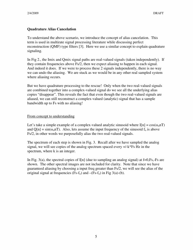
Quadrature Alias Cancelation

To understand the above scenario, we introduce the concept of alias cancelation. This

term is used in multirate signal processing literature while discussing perfect

reconstruction (QMF) type filters [3]. Here we use a similar concept to explain quadrature

signaling.

In Fig 2., the Imix and Qmix signal paths are real-valued signals (taken independently). If

they contain frequencies above Fs/2, then we expect aliasing to happen in each signal.

And indeed it does. If we were to process these 2 signals independently, there is no way

we can undo the aliasing. We are stuck as we would be in any other real sampled system

where aliasing occurs.

But we have quadrature processing to the rescue! Only when the two real-valued signals

are combined together into a complex-valued signal do we see all the underlying alias

copies “disappear”. This reveals the fact that even though the two real-valued signals are

aliased, we can still reconstruct a complex-valued (analytic) signal that has a sample

bandwidth up to Fs with no aliasing!

From concept to understanding

Let’s take a simple example of a complex-valued analytic sinusoid where I[n] = cos(ωonT)

and Q[n] = sin(ωonT). Also, lets assume the input frequency of the sinusoid fo is above

Fs/2, in other words we purposefully alias the two real-valued signals.

The spectrum of each step is shown in Fig. 3. Recall after we have sampled the analog

signal, we will see copies of the analog spectrum spaced every +/-k*Fs Hz in the

spectrum, where k is an integer.

In Fig. 3(a), the spectral copies of I[n] (due to sampling an analog signal) at f=0,Fs,-Fs are

shown. The other spectral images are not included for clarity. Note that since we have

guaranteed aliasing by choosing a input freq greater than Fs/2, we will see the alias of the

original signal at frequencies (Fs-fo) and –(Fs-fo) in Fig 3(a)-(b).

2/4/2009 DRAFT

6

Fig. 3 – Spectral description of quadrature alias cancelation

In Fig 3, step(a)-(b) shows the spectrum of the cos and sin signals, respectively. This is

easily verified using the Euler identities [1],[5]:

( )

( )tjtj

tjtj

eej

t

eet

ωω

ωω

ω

ω

−

−

−−

=

+=

2)sin(

2

1)cos(

(1.3)

The frequencies in our “sample band” of [-Fs/2, Fs/2] are shown to be alias frequencies of

(Fs-fo) and –(Fs-fo). In other words, these are the frequencies we would “see” in the

digital samples due to our aliasing. If we chose to process the real-signals separately, we

could not tell the true input frequency due to this aliasing.

Fs/2 Fs

-Fs/2 -Fs

original alias

I(f)

Fs

-Fs/2

-Fs

Q(f)

+j

-j

Fs/2

Fs -Fs/2 -Fs

orig

alias jQ(f)

Fs -Fs/2

-Fs

orig Z(f) = I(f) + jQ(f)

(a)

(b)

(c)

(d)

fo -fo

Fs/2

Re

Im

Sample band

f (Fs-fo) -(Fs-fo)

fo -(Fs-fo)

2/4/2009 DRAFT

7

In Eq (1.3), note that the spectrum of a sin is purely imaginary. Here we have shown this

on the imaginary “j” axis in Fig. 3(b).

In Fig. 3(c), the first step of creating the complex-valued signal is shown. Here, we are

defining Q(f) to be the imaginary part of the complex signal. Thus, we multiply Q(f) by

“j” as shown in 3(c). This multiplication rotates Q(f) by 90 degrees – placing it on the real

axis. Note that this is really a manifestation of complex math. The multiplication by “j”

re-defines mathematically the Q signal via a rotation. We are not physically rotating the

signal, but mathematically doing so in order to construct a tractable solution. Hence we

are choosing to view the two real-valued signals as one complex-valued signal.

In Fig 3(d). we combine both signals into a complex-valued signal Z(f) = I(f) + jQ(f).

Here is where the magic begins. By adding Fig. 3(a) with Fig. 3(c), we combine the two

real-valued signals into a complex representation. The result - we see the red “dotted”

alias copies subtract away! And the new complex-valued signal is analytic.

One can appreciate the remarkable result here. Even though we started out with two

aliased real-valued signals, we were able to combine them into a complex-valued signal

that canceled the alias images. The beneficial side effect of this cancelation is that we are

able to represent complex-valued signals up to frequencies of Fs. All of this is possible

because the complex signal is analytic and is no longer symmetric. One can see the

negative frequency term has vanished, thus it is not taking up bandwidth from [-Fs/2,0] as

it would in a real-valued signal.

Viewing the signal in the sample band

In this explanation the original input freq was > Fs/2. In Fig 3(d), we can see in our

sample band [-Fs/2, Fs/2] that we will detect a negative frequency. In other words, the

frequency we see in our discrete-time samples is actually a sinusoid at -(Fs–fo) Hz. Why?

Recall that we can only see into the spectral “window” (known as the sample band)

between [-Fs/2, Fs/2]. This is an artifact of the sampling theorem (everything outside of

this folds back down into the sampling band). Here we are “seeing” the analytic signal

copy from –Fs, which shows up in our sample band. The original frequency at fo is

outside our sample band, but we still get one of its spectral copies that falls into our

sample band. Plus the effective bandwidth of the signals we can uniquely determine is

still Fs Hz.

Now, this is only of concern if we were attempting to determine the frequency of the

complex-valued signal. This has no effect on the Nyquist relaxation criteria and is strictly

an artifact of complex signaling. We still get one frequency only in the sample band

(instead of 2 in the real signal case), and we know it to be –(Fs-fo). Thus we can still

solve for fo since we inherently know Fs.

The net effect is this: For any two real signals (in quadrature) with frequencies between

[0, Fs/2], the complex-valued spectrum will have a positive frequency impulse equal to fo.

For any two real signals (in quadrature) with frequencies between [Fs/2, Fs], the complex-

valued spectrum will have a negative frequency impulse equal to –(Fs-fo). The important

2/4/2009 DRAFT

8

fact here is that we can still uniquely determine fo up to frequencies equal to the sampling

frequency of Fs.

Simple example of a powerful concept

To drive the above explanation further, let’s try an example. From DSP theory we know

the DFT of any signal returns discrete frequency coefficients that represent in the input

signal frequency content from [-Fs/2, Fs/2].

Let’s take a sinusoid at fo=1kHz sampled at Fs=8kHz. We perform an FFT on this

sampled signal using MATLAB and take a look at the frequency response:

>> x=cos(2*pi*1000/8000*[0:N-1]);

>> X=fft(x);

>> f=[0:N-1]*8000/N - 4000;

>> plot(f,db(1/N*abs(fftshift(X))))

As expected, we see two frequency impulses at -1kHz and +1kHz for our real-valued

sinusoid. These are the only frequencies present in our [-4kHz, 4kHz] sample band. The

signal is also not aliased since we readily meet the sampling criteria.

Now consider a quadrature signal at fo=7kHz sampled at Fs=8kHz. Obviously, each real

signal is aliased since fo >Fs/2. As demonstrated in Fig. 3, we should expect to see an

analytic signal show up in our sample band at –(Fs-fo), which is equal to -1kHz.

>> x=cos(2*pi*7000/8000*[0:N-1]);

>> y=sin(2*pi*7000/8000*[0:N-1]);

2/4/2009 DRAFT

9

>> z=x+sqrt(-1)*y;

>> Z=fft(z);

>> plot(f,db(1/N*abs(fftshift(Z))))

In the above figure, we can indeed see we have a single complex exponential at -1kHz.

The above MATLAB commands look simple, but the underlying alias cancelation that

happened in Fig.3 was never truly seen. It all took place automatically! By referring to

Fig. 3, we can appreciate the mathematical steps that took place to create the final analytic

signal at -1kHz. And this is typically something that DSP engineers overlook (and for

good reason!).

Once you understand the concepts presented, then creating more complicated and

advanced quadrature systems is not very hard to accomplish.

Given the basis of quadrature signaling then we should be able to answer the original

questions:

1) Quadrature signaling effectively allows us to relax the Nyquist folding frequency

to Fs for analytic signals compared to the typical Fs/2 for real-valued signals.

2) This means if you are processing complex signals that have frequency content up

to Fs, the ADCs only have to sample at Fs rather than 2Fs (since we can cancel the

aliasing in the 2 real signals). In other words, the ADCs only have to run at half

the rate of a commensurate single real-valued sampling system.

2/4/2009 DRAFT

10

Phase and Amplitude Imbalance in Quadrature Signals

Another subject that is hardly discussed in DSP literature is the real-world implications of

imperfect quadrature signaling. As we have seen, if we have perfect analytic signals, then

the mathematics works out to our benefit. But what happens if the quadrature signal has

amplitude differences between the I and Q channel? What happens if the I and Q channel

are no longer 90 degrees out of phase relative to one another (no longer quadrature)?

In short, any amplitude or phase imbalance in the input quadrature signal will create

distortion. Quadrature imbalances void the analytic signal definition and create a situation

where system performance is limited to these errors. These sort of imperfections will

have consequences in digital communications, demodulation routines, and phase angle

detectors - just to name a few related DSP areas.

Phase imbalance

Let us first tackle phase imbalance. Here we start by assuming the quadrature signal has a

phase error offset of φ radians. We can push this entire error into the Q term since we are

worried about the relative phase between I and Q. We need the relative phase to be 90

degrees for a purely analytic signal, and any imbalance will show an error in the relative

phase between I and Q.

In this case it can be shown that the imbalanced complex-valued signal takes on the form:

)sin()cos()( φωωφ ++= tjttA (1.6)

And put into complex exponential notation Eq. (1.6) becomes:

[ ])1()1(2

1)( φωφω

φjtjjtj

eeeetA−− −⋅++⋅= (1.7)

Eq (1.7) shows that Aφ(t) is no longer analytic, but is rather symmetric and complex-

valued. It lies neither on the real or imaginary frequency axis, but somewhere inbetween.

The spectrum of Aφ(t) also has positive and negative frequency terms at w and -w, similar

to a real-valued sinusoid.

NOTE: If we substitute φ=0, you can see that Eq. (1.7) turns back into its analytic tje

ω ,

which is what we expect with no phase imbalance.

Eq. (1.7) gives us a tool to assess what happens when the input signal to a quadrature

mixer has a phase imbalance. It tells us that the phase imbalance creates a negative

frequency image scaled by a complex number )1(2

1 φje

−− . Also, the positive frequency is

scaled - it decreases as the phase imbalance angle increases. Thus for increasing phase

imbalance, the negative freq image gets stronger and the positive freq gets weaker. If

φ=π, we can see that the negative freq image has unity amplitude, and the positive

frequency image disappears. Since the phase angle offset directly affects the strength of

2/4/2009 DRAFT

11

the image frequency, it governs the amount of alias cancelation we will see when we

attempt to combine the real signals into a complex-valued waveform.

Recall for an analytic signal, the absence of negative frequencies is due to the fact that

they directly canceled during the analytic signal derivation. With a phase imbalance, now

these negative frequency “images” will not completely cancel and will be directly

proportional to the phase angle imbalance between the incoming analog signals.

If you reference Fig. 3c, remember when we multiplied the Q signal by “j”, it effectively

rotated the signal 90 degrees so it lined up with the real axis (since it was originally on the

imaginary axis). As such, adding Fig. 3a with Fig. 3c resulted in a spectrum that resided

on the real axis, and the negative (alias) images fully canceled. With a phase imbalance,

you can imagine that the Q signal is no longer aligned on the imaginary axis, but it offset

from it. So rotating this imbalanced Q signal 90 degrees does not align it on the real axis,

but offset from it by φ degrees. When you add the real and imaginary signals, you have to

do vector addition [5] on the I and Q spectral graphs, and you will see that the real part of

the composite quadrature signal is no longer on the real axis. The result is that a portion

of the negative (alias) frequency image remains due to incomplete cancelation.

The phase imbalanced quadrature signal has a frequency response given by:

)]()([2

)()sin(][

)]()([2

1)()cos(][

oo

j

o

ooo

ffffej

fQnTnQ

fffffInTnI

+−−−=⇔+=

++−=⇔=

δδϕω

δδω

ϕ

For the Q signal, we see the delta functions do not lie strictly on the “j” axis, but are now

scaled by ϕje , effectively moving them off the “j” axis.

Next is a plot showing what happens during the complex signal construction with a phase

offset angle equal to φ. We use the same signal as in Fig. 3, where the real-valued I and Q

signals are at fo>Fs/2 (purposefully aliased). This can be done without loss of generality.

NOTE: If the I and Q signals do not violate the sampling theorem (fo<Fs/2), then the

same cancelation issue arises. As a formality, we don’t refer to it as alias cancelation. We

want to cancel the negative frequency images, which are not aliased in that case. But the

concept is really the same - we are attempting to make the negative images in the real

signals “disappear” through construction combination of the real-valued signals.

2/4/2009 DRAFT

12

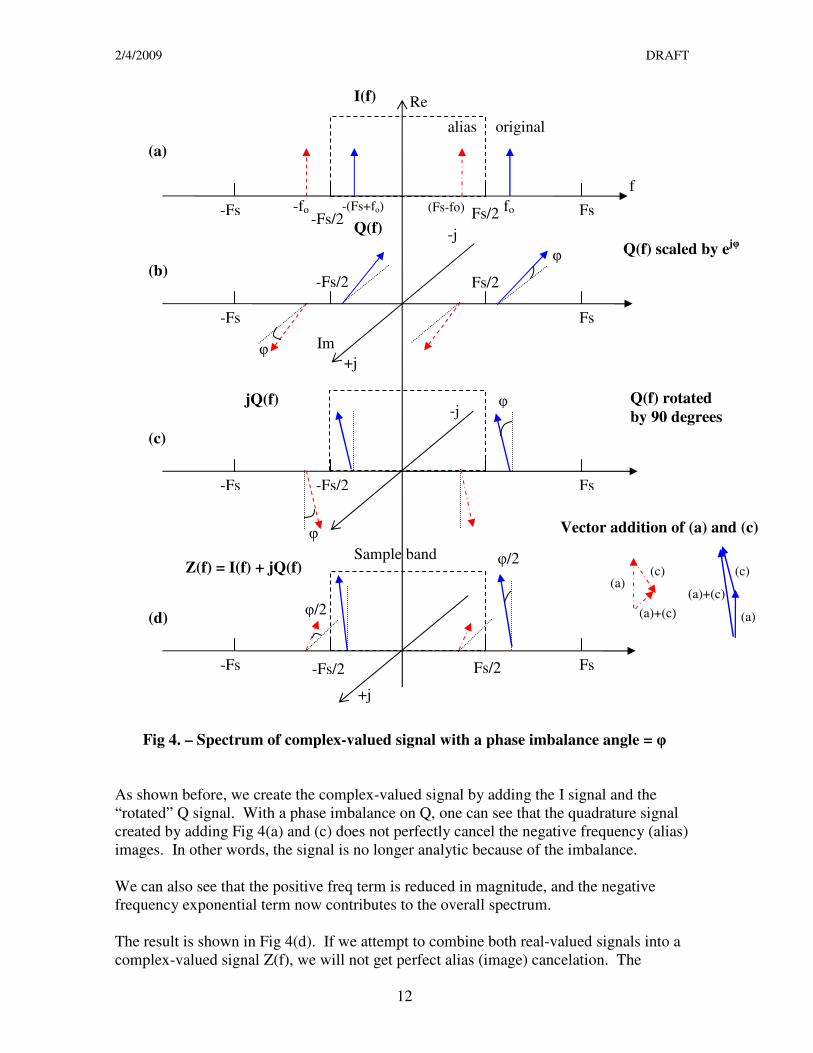
Fig 4. – Spectrum of complex-valued signal with a phase imbalance angle = φ

As shown before, we create the complex-valued signal by adding the I signal and the

“rotated” Q signal. With a phase imbalance on Q, one can see that the quadrature signal

created by adding Fig 4(a) and (c) does not perfectly cancel the negative frequency (alias)

images. In other words, the signal is no longer analytic because of the imbalance.

We can also see that the positive freq term is reduced in magnitude, and the negative

frequency exponential term now contributes to the overall spectrum.

The result is shown in Fig 4(d). If we attempt to combine both real-valued signals into a

complex-valued signal Z(f), we will not get perfect alias (image) cancelation. The

Fs/2 Fs -Fs/2

-Fs

original alias

I(f)

Fs

-Fs/2

-Fs

Q(f)

+j

-j

Fs/2

Fs -Fs/2 -Fs

jQ(f)

Fs -Fs/2 -Fs

Z(f) = I(f) + jQ(f)

(a)

(b)

(c)

(d)

fo -fo

Fs/2

Re

Im

Sample band

f

(Fs-fo)

φ

φ

Vector addition of (a) and (c)

Q(f) rotated

by 90 degrees

φ/2

φ/2

φ

Q(f) scaled by ejφ

-j

+j

(a) (c)

(a)+(c) (a)

(c)

(a)+(c)

φ

-(Fs+fo)

2/4/2009 DRAFT

13

negative frequency term in the sample band will be seen as distortion in our resultant

quadrature signal. This violates our assumption that the complex-valued signal will be

analytic. And because it is no longer analytic, we will not be able to resolve (without

ambiguity) frequencies in the [Fs/2, Fs] band (even though the resultant signal is complex-

valued).

Amplitude imbalance

If the quadrature input signal also has some amplitude error between the I and Q channels,

this also couples with the phase imbalance. Amplitude imbalance also creates disortion in

the form of a negative frequency image.

Let’s now write a quadrature signal with a phase offset of φ radians, the I channel with an

amplitude of α, and the Q channel with an amplitude of β.

)sin()cos()( φωβωα ++= tjttA (1.8)

Eq. (1.8) can also be written in complex-form as:

[ ])()(2

1)( φωφω βαβα jtjjtj

eeeetA−− −⋅++⋅= (1.9)

As before in the phase imbalance case, the signal is no longer analytic and the negative

frequency image (that is seen as a distortion in the output) has a magnitude of:

)(2

1 φβα je

−− (1.10)

Thus we can see the amplitude imbalance terms also play a role in the magnitude of the

negative frequency image in the output complex-valued signal. The amplitude and phase

imbalances are indeed coupled and directly affect the strength of the negative frequency

image.

Of course, if we make α=β, then Eq. (1.9) is equal to Eq. (1.7) with a simple scaling

factor. Also note that for α=β and φ=0, Eq. (1.9) still reduces to the well-known complex

exponential.

2/4/2009 DRAFT

14

Digital Quadrature Phase Balancing

To address phase balancing, we go back to our mixdown example in Fig. 2, where the

input signal is a complex sinusoid being mixed down to an intermediate frequency (IF).

To rectify any phase and amplitude imbalance in the input signal, it turns out that we can

correct these in the digital domain before the complex mix to baseband. Thus, we can

take an ill-formed analog (or digital) quadrature signal and “fix” it with DSP techniques!

Let’s first consider the phase balancing task by itself. Here we will assume there is no

amplitude imbalance (we will see later it can be added in the path without loss of

generality).

The first task is to estimate the phase imbalance angle φ. Once we have estimated this

parameter, we can correct for it digitally. There are several methods on how to do this

phase correction – two such methods are proposed. Estimating the phase imbalance angle

will be presented after the methods of how to actually “fix” the imbalance.

Method 1:

The first method involves using a fractional-delay filter to delay the Q channel. In this

setup, the phase imbalance φ is used to determine how many samples we must delay the Q

channel with respect to the I channel to maintain a 90-degree phase relationship.

With this method we would be delaying the Q channel by “d” samples, where d is not

constrained to be an integer:

Qcorr (n) = Q(n-d), where d = φ/2πfT

The fractional-delay filter will have a total delay D = d + N. The FIR delay “N” is the

inherent delay in the filter itself (related to the number of filter taps), and this delay is

added to the desired fractional delay term to create “total delay” D.

Here is a block diagram:

2/4/2009 DRAFT

15

Fig. 5 – Fractional-delay FIR filter for phase correction

The fractional-delay filter shown in Fig.5 would be generated once the system has

estimated the phase imbalance term. The delay z-N

in the I signal path is strictly there to

time align the 2 signals. Since the Q term will be inherently delayed due to the FIR filter

in it’s path, we must also delay the I term by the integer number of samples due to the

filter delay (N). The composite delay leftover between I and Q will be the fractional delay

“d” we wanted.

A low-order FIR filter could be generated using Lagrange interpolation coeffs for the

fractional-delay filter [4]:

∏≠=

=−

−=

N

nkk

Nnkn

kDnh

0

,...,2,1,0,][

This filter has a great approximation for low frequencies and the filter coefficients are

easy to compute. But there is a phase delay vs. magnitude response tradeoff with this

cos(ωot) ADC )cos( nTcω

)sin( nTcω sin(ωot + φ)

ADC

)cos( nTcω

)sin( nTcω

+

+

Qmix

Imix

digital Filtered phase balancing

and mix operation analog

+

-

Frac-delay

Filter H(z)

estimated φ

z-N

2/4/2009 DRAFT

16

filter structure. Other filters can be used here to meet the necessary specs – including a

least squares filter or a polyphase fractional-delay structure.

Method 2:

The second method of phase correction comes from the serendipitous application of the

basic trig identity:

)sin()cos()cos()sin()sin( bababa +=+

In which if we apply to our phase imbalance signal on the Q channel:

)sin()cos()cos()sin()sin( φωφωφω ttt +=+

Now we can solve for sin(ωt), which is the desired output we wish to generate given our

phase-imbalanced input signal:

)cos(

)sin()cos()sin()sin(

φ

φωφωω

ttt

−+= (1.11)

And referring to Eq. 1.1b, since cos(ωt) = I channel and sin(ωt+φ) = Q channel, we can

use these two inputs to generate a corrected Q signal via:

)cos(

)sin()sin(

φ

φω

⋅−==

IQQt corr (1.12)

Where the phase imbalance angle φ would again be estimated using digital samples.

Since cos(φ) is always less than or equal to one, that means the denominator term in (1.12)

will be greater than one, which is not easily implemented in fixed-pt hardware. Thus if

we are implementing this on a fixed-pt FPGA or DSP, we must rewrite this equation to be

implemented in fixed-pt (integer) math. One equation to use is:

( ) ( ) )(cfsfIQsfIQQcorr ⋅⋅−+⋅−= (1.12b)

Where: sf = sin(φ) and cf = ( 1/cos(φ)-1 ), if 0<φ<60 deg

This “direct method” of phase correction calls for 2 multiplies and 2 adds, and can be

readily implemented inside an FPGA or DSP. Also note we can turn off this correction by

setting the factors sf = 0 and cf = 0.

Next is a block diagram of the direct method:

2/4/2009 DRAFT

17

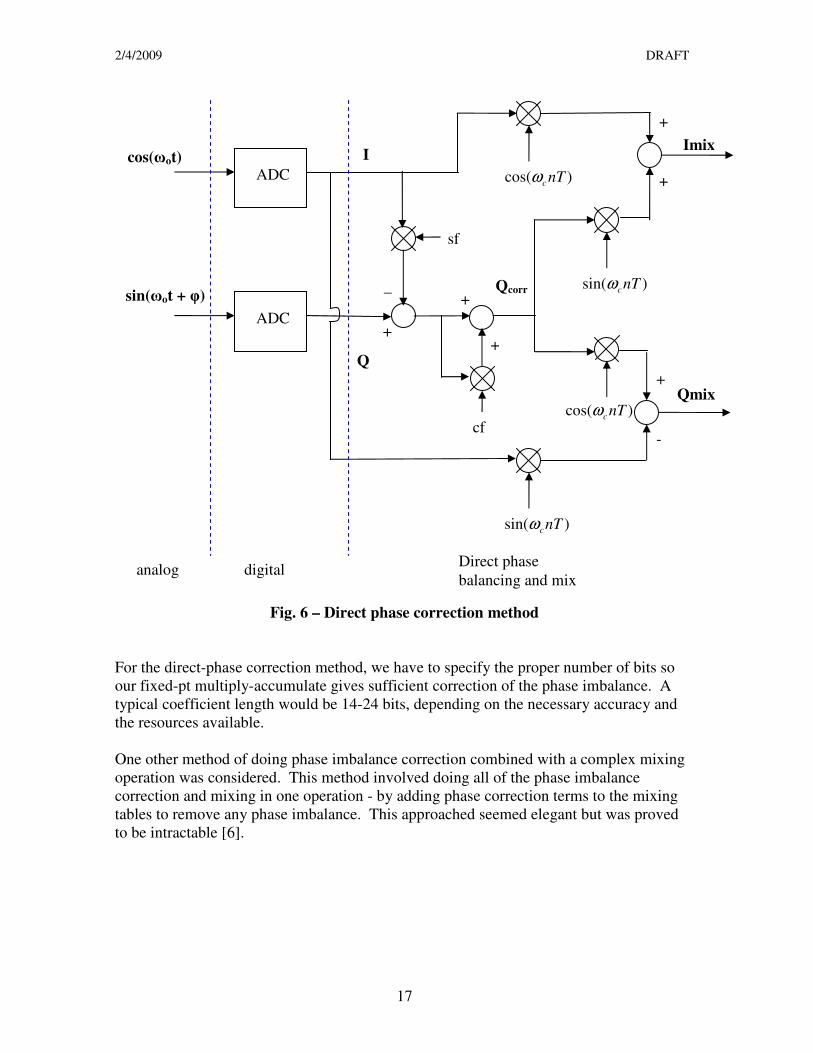
Fig. 6 – Direct phase correction method

For the direct-phase correction method, we have to specify the proper number of bits so

our fixed-pt multiply-accumulate gives sufficient correction of the phase imbalance. A

typical coefficient length would be 14-24 bits, depending on the necessary accuracy and

the resources available.

One other method of doing phase imbalance correction combined with a complex mixing

operation was considered. This method involved doing all of the phase imbalance

correction and mixing in one operation - by adding phase correction terms to the mixing

tables to remove any phase imbalance. This approached seemed elegant but was proved

to be intractable [6].

cos(ωot) ADC )cos( nTcω

)sin( nTcω sin(ωot + φ)

ADC

)cos( nTcω

)sin( nTcω

+

+

Qmix

Imix

digital Direct phase

balancing and mix analog

+

-

sf

+

_

cf

+

+

Qcorr

I

Q

2/4/2009 DRAFT

18

Phase Imbalance Estimation

We already have a method for correcting the phase of the input quadrature signal, but we

first must estimate the actual phase imbalance angle φ. This estimation is more readily

done in a DSP or other processor where multiple time-series digital samples can be

analyzed.

One of the simplest methods is to treat the I and Q signals as vectors in Nth

-dimensional

space. Since each signal can be defined as an element in Hilbert space, then we can use

the definition on the inner (dot) product to estimate the angle between the two signals.

Hence,

)cos(, θ⋅⋅= baba (1.13)

Where the modulus is defined as: ),( aasqrta =

To find the phase angle between the incoming I and Q signals, simply use the dot product

definition over the number of samples collected.

Let us define the inner product in Hilbert space (where I and Q can be complex),

∑−

=

=1

0

*,N

k

kkQIQI , and N = number of samples collected

And,

= ∑

−

=

1

0

2N

k

kIsqrtI ,

= ∑

−

=

1

0

2N

k

kQsqrtQ

Solving for the phase angle in Eq. (1.13),

⋅= −

QI

QI ,cos 1θ (1.14)

θπ

φ −=∴2

These operations are easily done on incoming complex-valued data samples. Also note

that this is not a temporal operation, but a vector operation. Hence we do not need

contiguous data samples for this method to work, we just need N samples of the signal in

order to estimate the phase angle (fragmented or contiguous).

Once we have determined the phase imbalance angle φ, we can set the sin() and cos()

factors to correct the digital Q signal. Once this is done, the incoming analog signal will

now be forced to have a 90-degree separation (analytic), and the resulting complex mix

will be free from negative frequency images due to phase imbalances.

2/4/2009 DRAFT

19

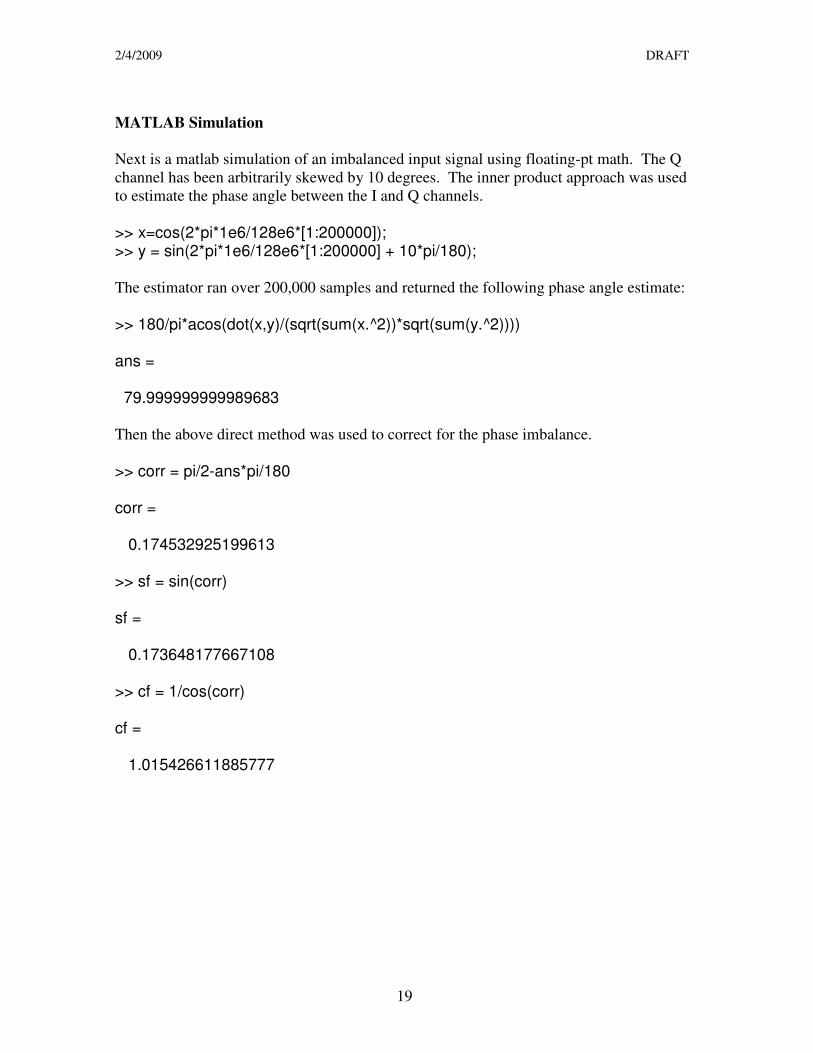
MATLAB Simulation

Next is a matlab simulation of an imbalanced input signal using floating-pt math. The Q

channel has been arbitrarily skewed by 10 degrees. The inner product approach was used

to estimate the phase angle between the I and Q channels.

>> x=cos(2*pi*1e6/128e6*[1:200000]); >> y = sin(2*pi*1e6/128e6*[1:200000] + 10*pi/180);

The estimator ran over 200,000 samples and returned the following phase angle estimate:

>> 180/pi*acos(dot(x,y)/(sqrt(sum(x.^2))*sqrt(sum(y.^2)))) ans = 79.999999999989683

Then the above direct method was used to correct for the phase imbalance.

>> corr = pi/2-ans*pi/180 corr = 0.174532925199613 >> sf = sin(corr) sf = 0.173648177667108 >> cf = 1/cos(corr) cf = 1.015426611885777

2/4/2009 DRAFT

20

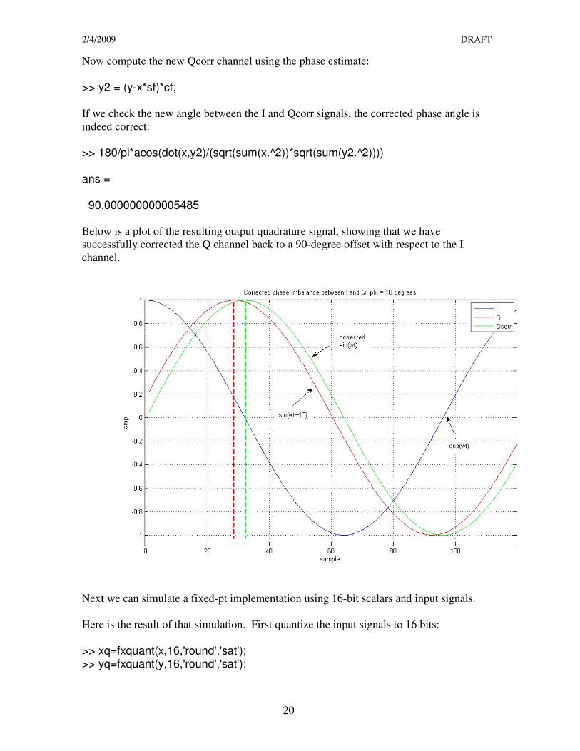
Now compute the new Qcorr channel using the phase estimate:

>> y2 = (y-x*sf)*cf;

If we check the new angle between the I and Qcorr signals, the corrected phase angle is

indeed correct:

>> 180/pi*acos(dot(x,y2)/(sqrt(sum(x.^2))*sqrt(sum(y2.^2)))) ans = 90.000000000005485

Below is a plot of the resulting output quadrature signal, showing that we have

successfully corrected the Q channel back to a 90-degree offset with respect to the I

channel.

Next we can simulate a fixed-pt implementation using 16-bit scalars and input signals.

Here is the result of that simulation. First quantize the input signals to 16 bits:

>> xq=fxquant(x,16,'round','sat'); >> yq=fxquant(y,16,'round','sat');

2/4/2009 DRAFT

21

>> 180/pi*acos(dot(xq,yq)/(sqrt(sum(xq.^2))*sqrt(sum(yq.^2)))) ans = 79.999843652984907

The estimated phase angle is accurate to 1e-4 degrees using 16-bit input samples in the

phase angle estimator.

>> corr = pi/2-ans*pi/180 corr = 0.174535653969622 >> sf = sin(corr)

sf = 0.173650864980322 >> sf = fxquant(sf,16,'round','sat') sf = 0.173645019531250 >> cf = 1/cos(corr) cf = 1.015427100468173 Here we take 1/cos(φ)-1 as outlined before for a fixed-pt implementation:

>> cfq = fxquant(cf-1,16,'round','sat') cfq = 0.015441894531250

2/4/2009 DRAFT

22

Here is the correction done in the FPGA using 16-bit fixed pt multiplies, utilizing Eq.

(1.4b):

>> y2q = fxquant((yq-fxquant(xq*sf,16,'round','sat'))*(1+cfq),16,'round','sat'); Checking our result gives us the corrected phase angle between I and Qcorr:

>> 180/pi*acos(dot(xq,y2q)/(sqrt(sum(xq.^2))*sqrt(sum(y2q.^2)))) ans = 89.999550699810129

So using the proposed fixed-pt implementation with 16-bit samples and multiplies, we

still get a phase angle correction accurate down to 1e-4 degrees.

Digital Quadrature Amplitude Balancing

Up to this point we have brushed aside the amplitude imbalance issue. The reason for this

is that our phase balancing derivation assumed equal amplitudes. So if we simply scale

the I and Q channels to have equal amplitudes and pass the resulting signals to the phase

correction block, we will have solved the coupled problem of phase and amplitude

balancing.

Amplitude correction is easily implemented in a similar fashion by estimating the

envelope of the I and Q signals and correcting them with scalar multiplies before the

phase correction block. We can also push the relative amplitude difference into the Q

term to rid of one extra multiply.

Figure 7 shows one such block diagram that does amplitude correction first, then phase

correction.

2/4/2009 DRAFT

23

Fig. 7 – Amplitude and phase correction for imbalanced quadrature input

In determining the amplitudes α and β for the I and Q signals, one can use a similar

approach to the imbalance phase angle estimation. This time we can look at a contiguous

time series of “N” digital samples. If we assume again we are expecting sinusoidal input,

we can use Parseval’s theorem to compute amplitude from power. Recall Parseval’s

theorem states that power computed in the frequency domain and time domain are equal.

As such, we can compute power (given a zero-mean signal) via:

21

0

])[(1

nxN

PN

n

o ∑−

=

= “Parseval’s theorem”

2

2A

Po = “power in a sinusoid” (1.15)

First compute the power Po over N pts, then solve for the amplitude “A” of the sinusoid

using Eq. (1.15).

NOTE: The above approach guarantees that you will get the “true” amplitude. Consider

if you simply tried to look at the max and min samples of your signal to determine the

amplitude. Then you might not ever see the true max or min amplitude value. In fact,

there are certain frequency relationships between input and sample frequency where you

will never see the true max and min amplitudes in the digital samples! The above

approach mitigates this issue altogether.

αcos(wot) ADC

βsin(wot+φ) ADC

Quadrature amplitude and

phase correction analog

sf

+

_

cf

+

+

Qcorr

I

Q α/β

Icorr

2/4/2009 DRAFT

24

Conclusion

This article focused on quadrature signaling and the definition of complex-valued signals

with respect to real-world inputs. It was shown how real signals are combined into

complex signals, and the folklore behind the advantages of quadrature signaling were

methodically proven. Furthermore, the effects of phase and amplitude imbalances in

quadrature signals were explored, and methods for compensating these imbalances were

discussed.

References

[1] R. Lyons, Understanding Digital Signal Processing, Prentice-Hall PTR, Upper

Saddle River, NJ, 2001, Appendix C

[2] S. Mitra and J. Kaiser, Handbook for Digital Signal Processing, John Wiley & Sons,

New York, 1993, Ch. 13

[3] P. Vaidyanathan, Multirate Systems and Filter Banks, Prentice-Hall, Upper Saddle

River, NJ, 1993

[4] T. Laakso, V. Valimaki, M. Karjalainen, U. Laine, Splitting the Unit Delay, IEEE

Signal Processing Magazine, Jan. 1996

[5] R. Churchill and J. Brown, Complex Variables and Applications, 5th

edition,

McGraw-Hill, 1990

2/4/2009 DRAFT

25

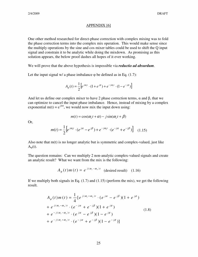
APPENDIX [6]

One other method researched for direct-phase correction with complex mixing was to fold

the phase correction terms into the complex mix operation. This would make sense since

the multiply operations by the sine and cos mixer tables could be used to shift the Q input

signal and constrain it to be analytic while doing the mixdown. As promising as this

solution appears, the below proof dashes all hopes of it ever working.

We will prove that the above hypothesis is impossible via reductio ad absurdum.

Let the input signal w/ a phase imbalance φ be defined as in Eq. (1.7):

[ ])1()1(2

1)( φωφω

φjtjjtj

eeeetA cc −− −⋅++⋅=

And let us define our complex mixer to have 2 phase correction terms, α and β, that we

can optimize to cancel the input phase imbalance. Hence, instead of mixing by a complex

exponential m(t) = e-jwt

, we would now mix the input down using:

)sin()cos()( βωαω +−+= tjttm oo

Or,

[ ])()(2

1)( βαωβαω jjtjjjtj

eeeeeetm oo −−− +⋅+−⋅= (1.15)

Also note that m(t) is no longer analytic but is symmetric and complex-valued, just like

Aφ(t).

The question remains: Can we multiply 2 non-analytic complex-valued signals and create

an analytic result? What we want from the mix is the following:

tj ocetmtA

)()()(

ωωφ

−= (desired result) (1.16)

If we multiply both signals in Eq. (1.7) and (1.15) (perform the mix), we get the following

result.

)]1)((

)1)((

)1)((

)1)(([4

1)()(

)(

)(

)(

)(

φβαωω

φβαωω

φβαωω

φβαωωφ

jjjtj

jjjtj

jjjtj

jjjtj

eeee

eeee

eeee

eeeetmtA

oc

oc

oc

oc

−−−+−

−−

−−−

+

−+⋅+

−−⋅+

++⋅+

+−⋅=

(1.8)

2/4/2009 DRAFT

26

From this mix operation, we can see we only want to keep the 2nd

term, which is the

desired analytic complex exponential in Eq. (1.1b), but scaled by a complex value. All

other terms are images we want to suppress if we want a true analytic output signal.

We can write the following set of constraints to achieve the desired signal as in Eq (1.1b):

(1) 0)1()1( =+−+ φβφα jjjjeeee

(2) λφβφα jjjjj eeeee 4)1()1( =+++ −−

(3) 0)1()1( =−−− −− φβφα jjjjeeee

(4) 0)1()1( =−+− −−−− φβφα jjjj eeee

Uniquely solving these 4 constraints will create an analytic signal and rid of the offending

images due to the phase imbalance.

One can see that constraints (1) and (3) require that:

βα jj

ee = , or πβα n2+=

Whereas constraint (4) requires: βα jj

ee−− −=

Plugging in for α: βπβ jnj

ee−+− −=)2(

11 −=

Which is a contradiction! Therefore there does not exist any (α, β) pair to solve the

problem.

In short, we cannot cancel out all the images in the mixing operation while simultaneously

creating an analytic result. We must fix the phase imbalance before mixing. The above

has proved that two non-analytic complex-valued signals cannot be mixed together with

the side-effect of generating a purely analytic result.