quadratic programming maxcut primal and dual sdp...
TRANSCRIPT

3 - 1 Quadratically Constrained Quadratic Programming P. Parrilo and S. Lall, CDC 2003 2003.12.07.01
3. Quadratically Constrained Quadratic Programming
• Quadratic programming
• MAXCUT
• Boolean optimization
• Primal and dual SDP relaxations
• Randomization
• Interpretations
• Examples
• LQR with binary inputs
• Rounding schemes
3 - 2 Quadratically Constrained Quadratic Programming P. Parrilo and S. Lall, CDC 2003 2003.12.07.01
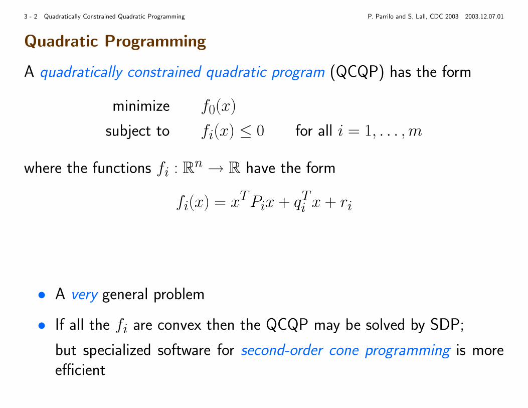
Quadratic Programming
A quadratically constrained quadratic program (QCQP) has the form
minimize f0(x)
subject to fi(x) ≤ 0 for all i = 1, . . . ,m
where the functions fi : Rn→ R have the form
fi(x) = xTPix + qTi x + ri
• A very general problem
• If all the fi are convex then the QCQP may be solved by SDP;
but specialized software for second-order cone programming is moreefficient
3 - 3 Quadratically Constrained Quadratic Programming P. Parrilo and S. Lall, CDC 2003 2003.12.07.01
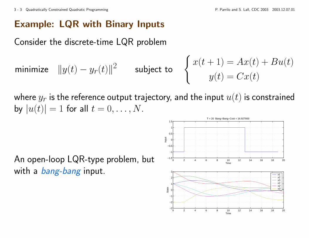
Example: LQR with Binary Inputs
Consider the discrete-time LQR problem
minimize ‖y(t)− yr(t)‖2 subject to
{x(t + 1) = Ax(t) + Bu(t)
y(t) = Cx(t)
where yr is the reference output trajectory, and the input u(t) is constrainedby |u(t)| = 1 for all t = 0, . . . , N .
An open-loop LQR-type problem, butwith a bang-bang input.
0 2 4 6 8 10 12 14 16 18 20−1.5
−1
−0.5
0
0.5
1
1.5
TimeIn
put
T = 20 Bang−Bang−Cost = 16.927000
0 2 4 6 8 10 12 14 16 18 20−3
−2
−1
0
1
2
3
Time
Sta
te
x1x2x3x1’x2’x3’
3 - 4 Quadratically Constrained Quadratic Programming P. Parrilo and S. Lall, CDC 2003 2003.12.07.01
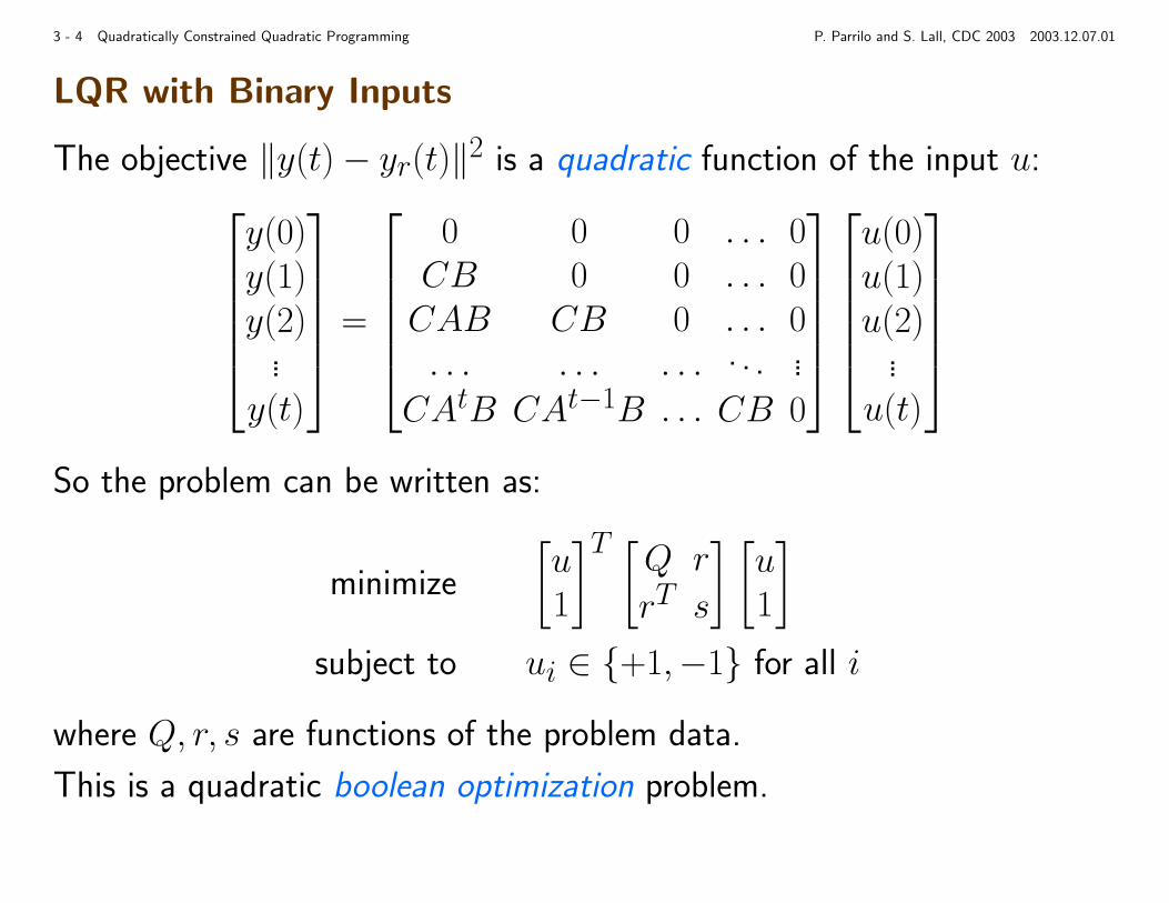
LQR with Binary Inputs
The objective ‖y(t)− yr(t)‖2 is a quadratic function of the input u:
y(0)y(1)y(2)
...y(t)
=
0 0 0 . . . 0CB 0 0 . . . 0CAB CB 0 . . . 0. . . . . . . . . . . . ...
CAtB CAt−1B . . . CB 0
u(0)u(1)u(2)
...u(t)
So the problem can be written as:
minimize
[u1
]T [Q r
rT s
] [u1
]
subject to ui ∈ {+1,−1} for all i
where Q, r, s are functions of the problem data.
This is a quadratic boolean optimization problem.

3 - 5 Quadratically Constrained Quadratic Programming P. Parrilo and S. Lall, CDC 2003 2003.12.07.01
MAXCUT
given an undirected graph, with no self-loops
• vertex set V = { 1, . . . , n }
• edge set E ⊂{{i, j} | i, j ∈ V, i 6= j
}
For a subset S ⊂ V , the capacity of S is the number of edges connectinga node in S to a node not in S
the MAXCUT problem
find S ⊂ V with maximum capacity
the example above shows a cut with capacity 15; this is the maximum

3 - 6 Quadratically Constrained Quadratic Programming P. Parrilo and S. Lall, CDC 2003 2003.12.07.01
Example
a graph with 12 nodes, 24 edges; the maximum capacity cmax = 20
3 - 7 Quadratically Constrained Quadratic Programming P. Parrilo and S. Lall, CDC 2003 2003.12.07.01
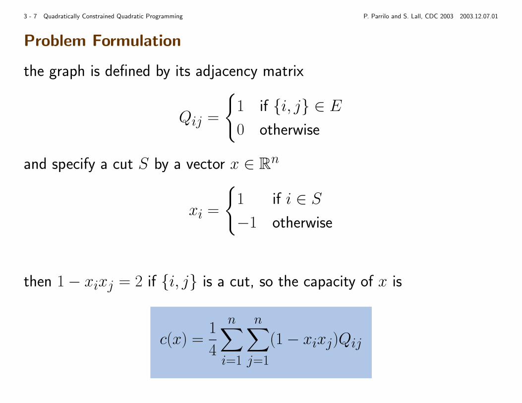
Problem Formulation
the graph is defined by its adjacency matrix
Qij =
{1 if {i, j} ∈ E0 otherwise
and specify a cut S by a vector x ∈ Rn
xi =
{1 if i ∈ S−1 otherwise
then 1− xixj = 2 if {i, j} is a cut, so the capacity of x is
c(x) =1
4
n∑
i=1
n∑
j=1
(1− xixj)Qij

3 - 8 Quadratically Constrained Quadratic Programming P. Parrilo and S. Lall, CDC 2003 2003.12.07.01
Optimization Formulation
so we’d like to solve
minimize xTQx
subject to xi ∈ {−1, 1 } for all i = 1, . . . , n
call the optimal value p?, then the maximum cut is
cmax =1
4
n∑
i=1
n∑
j=1
Qij −1
4p?
3 - 9 Quadratically Constrained Quadratic Programming P. Parrilo and S. Lall, CDC 2003 2003.12.07.01
Boolean Optimization
A classic combinatorial problem:
minimize xTQx
subject to xi ∈ {−1, 1}
• Many other examples; knapsack, LQR with binary inputs, etc.
• Can model the constraints with quadratic equations:
x2i − 1 = 0 ⇐⇒ xi ∈ {−1, 1}
• An exponential number of points. Cannot check them all!
• The problem is NP-complete (even if Q º 0).
Despite the hardness of the problem, there are some very good approaches. . .
3 - 10 Quadratically Constrained Quadratic Programming P. Parrilo and S. Lall, CDC 2003 2003.12.07.01
SDP Relaxations
We can find a lower bound via the dual; the primal is
minimize xTQx
subject to x2i − 1 = 0
Let Λ = diag(λ1, . . . , λn), then the Lagrangian is
L(x, λ) = xTQx−n∑
i=1
λi(x2i − 1) = xT (Q− Λ)x + trace Λ
The dual is therefore the SDP
maximize trace Λ
subject to Q− Λ º 0
3 - 11 Quadratically Constrained Quadratic Programming P. Parrilo and S. Lall, CDC 2003 2003.12.07.01
SDP Relaxations
From this SDP we obtain a primal-dual pair of SDP relaxations
minimize traceQXsubject to X º 0
Xii = 1
maximize trace Λsubject to Q º Λ
Λ diagonal
• We derived them from Lagrangian and SDP duality
• But, these SDP relaxations arise in many other ways
• Well-known in combinatorial optimization, graph theory, etc.
• Several interpretations

3 - 12 Quadratically Constrained Quadratic Programming P. Parrilo and S. Lall, CDC 2003 2003.12.07.01
SDP Relaxations: Dual Side
Gives a simple underestimator of the objective function.
maximize trace Λ
subject to Q º Λ
Λ diagonal
Directly provides a lower bound on the objective: for any feasible x:
xTQx ≥ xTΛx =
n∑
i=1
Λiix2i = trace Λ
• The first inequality follows from Q º Λ
• The second equation from Λ being diagonal
• The third, from xi ∈ {+1,−1}

3 - 13 Quadratically Constrained Quadratic Programming P. Parrilo and S. Lall, CDC 2003 2003.12.07.01
SDP Relaxations: Primal Side
The original problem is:
minimize xTQx
subject to x2i = 1
Let X := xxT . Then
xTQx = traceQxxT = traceQX
Therefore, X º 0, has rank one, and Xii = x2i = 1.
Conversely, any matrix X with
X º 0, Xii = 1, rankX = 1
necessarily has the form X = xxT for some ±1 vector x.
3 - 14 Quadratically Constrained Quadratic Programming P. Parrilo and S. Lall, CDC 2003 2003.12.07.01
Primal Side
Therefore, the original problem can be exactly rewritten as:
minimize traceQX
subject to X º 0
Xii = 1
rank(X) = 1
Interpretation: lift to a higher dimensional space, from Rn to Sn.
Dropping the (nonconvex) rank constraint, we obtain the relaxation.
If the solution X has rank 1, then we have solved the original problem.
Otherwise, rounding schemes to project solutions. In some cases, approxi-mation guarantees (e.g. Goemans-Williamson for MAX CUT).

3 - 15 Quadratically Constrained Quadratic Programming P. Parrilo and S. Lall, CDC 2003 2003.12.07.01
Feasible Points and Certificates
minimize traceQXsubject to X º 0
Xii = 1
maximize trace Λsubject to Q º Λ
Λ diagonal
• Dual relaxations give certified bounds.
• Primal relaxations give information about possible feasible points.
• Both are solved simultaneously by primal-dual SDP solvers

3 - 16 Quadratically Constrained Quadratic Programming P. Parrilo and S. Lall, CDC 2003 2003.12.07.01
Example
minimize 2x1x2 + 4x1x3 + 6x2x3
subject to x2i = 1
The associated matrix is Q =
0 1 21 0 32 3 0
. The SDP solutions are:
X =
1 1 −11 1 −1−1 −1 1
, Λ =
−1 0 0
0 −2 00 0 −5
We have X º 0, Xii = 1, Q− Λ º 0, and
traceQX = trace Λ = −8
Since X is rank 1, from X = xxT we recover the optimal x =[1 1 −1
]T,
-1
-0.50
0.51p1
-1
-0.50
0.51
p2
-1
-0.5
0
0.5
1
p3
-1
-0.5
0
0.5
1
p3
3 - 17 Quadratically Constrained Quadratic Programming P. Parrilo and S. Lall, CDC 2003 2003.12.07.01
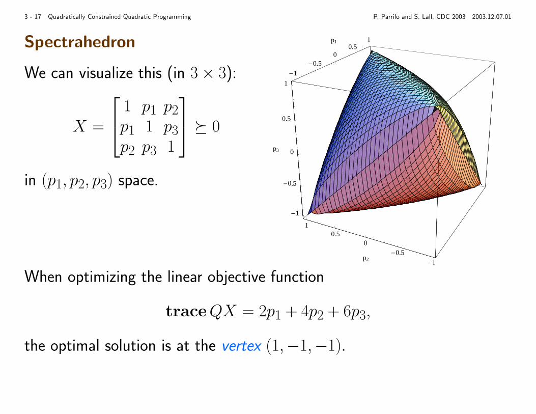
Spectrahedron
We can visualize this (in 3× 3):
X =
1 p1 p2p1 1 p3p2 p3 1
º 0
in (p1, p2, p3) space.
When optimizing the linear objective function
traceQX = 2p1 + 4p2 + 6p3,
the optimal solution is at the vertex (1,−1,−1).

3 - 18 Quadratically Constrained Quadratic Programming P. Parrilo and S. Lall, CDC 2003 2003.12.07.01
Primalization
After solving the SDP for X ∈ Sn, we’d like to map back to x ∈ {−1, 1}n
There may not exist an x ∈ {−1, 1}n such that X = xxT
We can interpret this
• algebraically: rankX 6= 1
• geometrically: X is not a lifted point
We need a procedure for finding a good x given X ; called rounding,primalization, or projection.
This is hard in general, but for MAXCUT good methods are known

3 - 19 Quadratically Constrained Quadratic Programming P. Parrilo and S. Lall, CDC 2003 2003.12.07.01
Randomization
Suppose we solve the primal relaxation
minimize traceQX
subject to X º 0
Xii = 1 for all i = 1, . . . , n
and the optimal X is not rank 1. Goemans and Williamson developed thefollowing randomized algorithm for finding a feasible point
• Factorize X as X = V TV , where V =[v1 . . . vn
]∈ Rr×n
• Then Xij = vTi vj, and since Xii = 1 this factorization gives n vectorson the unit sphere in Rr
• Instead of assigning either 1 or −1 to each vertex, we have assigneda point on the unit sphere in Rr to each vertex
3 - 20 Quadratically Constrained Quadratic Programming P. Parrilo and S. Lall, CDC 2003 2003.12.07.01
Randomized Slicing
Pick a random vector q ∈ Rr, and choose cut
S ={i | vTi q ≥ 0
}
Then the probability that {i, j} is a cut edge is
angle between vi and vjπ
=1
πarccos vTi vj
=1
πarccosXij
So the expected cut capacity is
csdp-expected =1
2
n∑
i=1
n∑
j=1
1
πQij arccosXij
−1 −0.5 0 0.5 10
0.5
1
1.5
2
2.5
3arcos(t)α(1−t)π/2
3 - 21 Quadratically Constrained Quadratic Programming P. Parrilo and S. Lall, CDC 2003 2003.12.07.01
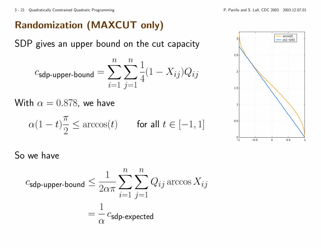
Randomization (MAXCUT only)
SDP gives an upper bound on the cut capacity
csdp-upper-bound =
n∑
i=1
n∑
j=1
1
4(1−Xij)Qij
With α = 0.878, we have
α(1− t)π2≤ arccos(t) for all t ∈ [−1, 1]
So we have
csdp-upper-bound ≤1
2απ
n∑
i=1
n∑
j=1
Qij arccosXij
=1
αcsdp-expected
3 - 22 Quadratically Constrained Quadratic Programming P. Parrilo and S. Lall, CDC 2003 2003.12.07.01
Randomization
So far, we have
• csdp-upper-bound ≤ 1α csdp-expected
• Also clearly csdp-expected ≤ cmax
• And cmax ≤ csdp-upper-bound
After solving the SDP, we slice randomly to generate a random family offeasible points.
We can sandwich the expected value of this family as follows. (α = 0.878)
αcsdp-upper-bound ≤ csdp-expected ≤ cmax ≤ csdp-upper-bound

3 - 23 Quadratically Constrained Quadratic Programming P. Parrilo and S. Lall, CDC 2003 2003.12.07.01
Coin-Flipping Approach
Suppose we just randomly assigned vertices to S with probability 12; then
ccoinflip-expected =1
4
n∑
i=1
n∑
j=1
Qij
A trivial upper bound on the maximum cut is just the total number of edges
ctrivial-upper-bound =1
2
n∑
i=1
n∑
j=1
Qij
and so ccoinflip-expected = 12ctrivial-upper-bound

3 - 24 Quadratically Constrained Quadratic Programming P. Parrilo and S. Lall, CDC 2003 2003.12.07.01
Coin-Flipping Approach
We have
• ccoinflip-expected = 12ctrivial-upper-bound
• ccoinflip-expected ≤ cmax
• cmax ≤ ctrivial-upper-bound
Again, we have a sandwich result
12ctrivial-upper-bound = ccoinflip-expected ≤ cmax ≤ ctrivial-upper-bound
3 - 25 Quadratically Constrained Quadratic Programming P. Parrilo and S. Lall, CDC 2003 2003.12.07.01
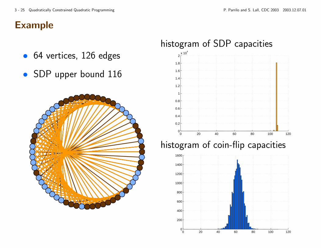
Example
• 64 vertices, 126 edges
• SDP upper bound 116
histogram of SDP capacities
0 20 40 60 80 100 1200
0.2
0.4
0.6
0.8
1
1.2
1.4
1.6
1.8
2x 10
4
histogram of coin-flip capacities
0 20 40 60 80 100 1200
200
400
600
800
1000
1200
1400
1600

3 - 26 Quadratically Constrained Quadratic Programming P. Parrilo and S. Lall, CDC 2003 2003.12.07.01
A General Scheme
Boolean Minimization
Relaxed X Dual-Bound ¤SDP
Duality
PrimalRelaxation
LagrangianDuality
• The relaxed X suggests candidate points.
• The diagonal matrix Λ certifies a lower bound.
Ubiquitous scheme in optimization (convex hulls, fractional colorings, etc. . . )
We will learn systematic ways of constructing these relaxations, and more. . .

3 - 27 Quadratically Constrained Quadratic Programming P. Parrilo and S. Lall, CDC 2003 2003.12.07.01
LQR with Binary Inputs
minimize
[u1
]T [Q r
rT s
] [u1
]
subject to ui ∈ {+1,−1} for all i
for some matrices (Q, r, s) function of the problem data (A,B,C,N).
An SDP dual bound:
maximize trace(Λ) + µ
subject to
[Q− Λ r
rT s− µ
]º 0, Λ diagonal
Let q∗, q∗ be the optimal value of both problems. Then, q∗ ≥ q∗:[u1
]T [Q r
rT s
] [u1
]≥[u1
]T [Λ 00 µ
] [u1
]= trace Λ + µ

3 - 28 Quadratically Constrained Quadratic Programming P. Parrilo and S. Lall, CDC 2003 2003.12.07.01
LQR with Binary Inputs
maximize trace(Λ) + µ
subject to
[Q− Λ r
rT s− µ
]º 0, Λ diagonal
Since (Λ, µ) = (0, 0) is always feasible, q∗ ≥ 0.
Furthermore, the bound is never worse than the LQR solution obtained bydropping the ±1 constraint, since
Λ = 0, µ = s− rTQ−1r
is a feasible point.
Example:
N LQR cost SDP bound Optimal10 14.005 15.803 15.80315 15.216 16.698 16.70520 15.364 16.905 16.927

3 - 29 Quadratically Constrained Quadratic Programming P. Parrilo and S. Lall, CDC 2003 2003.12.07.01
The S-procedure
A sufficient condition for the infeasibility of quadratic inequalities:
{x ∈ Rn | xTAix ≥ 0}
Again, a primal-dual pair of SDP relaxations:
X º 0traceX = 1
traceAiX ≥ 0
∑i λiAi ¹ −I
λi ≥ 0
The basis of many important results in control theory.
3 - 30 Quadratically Constrained Quadratic Programming P. Parrilo and S. Lall, CDC 2003 2003.12.07.01
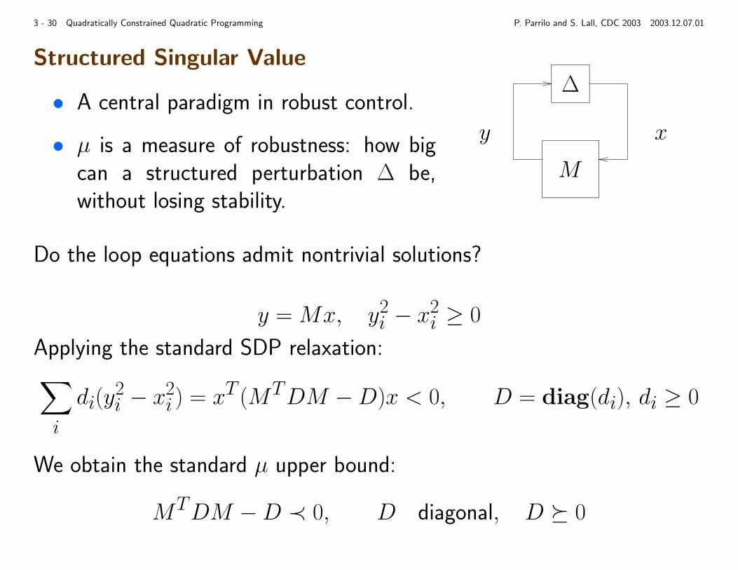
Structured Singular Value
• A central paradigm in robust control.
• µ is a measure of robustness: how bigcan a structured perturbation ∆ be,without losing stability.
∆
M
xy
Do the loop equations admit nontrivial solutions?
y = Mx, y2i − x2
i ≥ 0
Applying the standard SDP relaxation:∑
i
di(y2i − x2
i ) = xT (MTDM −D)x < 0, D = diag(di), di ≥ 0
We obtain the standard µ upper bound:
MTDM −D ≺ 0, D diagonal, D º 0