quadcopter obstacle avoidance using biomimetic algorithmseprints.whiterose.ac.uk/96477/1/as of obs...

This is a repository copy of Quadcopter Obstacle Avoidance using Biomimetic Algorithms.

White Rose Research Online URL for this paper:http://eprints.whiterose.ac.uk/96477/

Version: Submitted Version

Proceedings Paper:Sabo, C. and Simpson, A. (2016) Quadcopter Obstacle Avoidance using Biomimetic Algorithms. In: AIAA Infotech @ Aerospace, AIAA SciTec. AIAA Infotech@Aerospace, 04-08 Jan 2016, San Diego, CA. American Institute of Aeronautics and Astronautics . ISBN978-1-62410-388-9

https://doi.org/10.2514/6.2016-0403

© 2016 AIAA. This is an author produced version of a paper subsequently published in 'AIAA Infotech @ Aerospace' available at http://dx.doi.org/10.2514/6.2016-0403. Uploaded in accordance with the publisher's self-archiving policy.

[email protected]://eprints.whiterose.ac.uk/

Reuse Unless indicated otherwise, fulltext items are protected by copyright with all rights reserved. The copyright exception in section 29 of the Copyright, Designs and Patents Act 1988 allows the making of a single copy solely for the purpose of non-commercial research or private study within the limits of fair dealing. The publisher or other rights-holder may allow further reproduction and re-use of this version - refer to the White Rose Research Online record for this item. Where records identify the publisher as the copyright holder, users can verify any specific terms of use on the publisher’s website.

Takedown If you consider content in White Rose Research Online to be in breach of UK law, please notify us by emailing [email protected] including the URL of the record and the reason for the withdrawal request.

mailto:[email protected]

https://eprints.whiterose.ac.uk/

1 Undergraduate Student, Department of Aerospace Engineering 2 Postdoctoral Researcher, Department of Computer Science, AIAA Senior Member

MAV Obstacle Avoidance using Biomimetic Algorithms

Alexander Simpson1, Chelsea Sabo2 University of Sheffield, Sheffield, UK

Abstract

Unmanned Micro Aerial Vehicles (MAVs) have the potential to operate in diverse environments but are limited by the lack of robust algorithms for autonomous flight. This is largely due to the sensing and processing requirements that exceed the weight and power limitations of this hardware. Recent research has highlighted the potential to overcome these constraints by looking to the natural world, in particular to the possibilities of using optical flow. This work presents a novel biomimetic algorithm that uses optical flow data generated from the on-board camera of a quadcopter MAV to avoid obstacles in flight. Simulation results are presented showing the algorithm performance in a range of flying scenarios. This work also highlights the huge potential of using low resolution sensors and lightweight algorithms in the field of autonomous vehicle control.

I. Introduction

Unmanned Aerial Vehicles (UAVs) have increasingly diverse uses from search & rescue and environmental monitoring to military warfare and mine detection [1]. A UAV is preferable to a manned aircraft for any mission considered ‘dull, dirty or dangerous’ [2]. They have the potential to carry out complex tasks, such as conducting a systematic search or navigating a dense unfamiliar environment, with far greater accuracy and reliability than a human pilot. Between 2005 and 2012, the number of unmanned to manned aircraft operated by the United States Air Force increased from one-in-twenty to one-in-three [3], and these systems are seeing considerable worldwide research investment to develop their civil and military potential.

While technological advances in the aerodynamics, propulsion and materials science are improving UAVs all the time, the vast majority still rely on remote pilot operation. The main reason for this is that they have a limited payload capacity when compared with ground vehicles; this restricts the size, weight and power of sensors and processors that can be carried and imposes constraints on the complexity of algorithms they can employ.

The problem of autonomous control for UAVs has traditionally been regarded as a sub-field of robotics and control engineering, but recent research has highlighted the potential for exploiting solutions provided by nature [4]. Flying insects and animals are proof that virtuosic aerial proficiency does not require a huge brain or a multitude of sensors or masses of computing power. The goal of this research was to make use of the current level of understanding by developing a biomimetic algorithm that mimics object avoidance approaches used in the natural world. The performance of the algorithm was investigated with simulations conducted on videos of different flying scenarios. The following paper consists of a brief literature review, problem formulation, methodology, simulation, results and a discussion.

II. Literature

While UAV size, range and flight characteristics are improving rapidly, the same cannot be said of robust autonomous control techniques. Biomimetic approaches show the most promise to speed up progress in this area [4] [5]. A large proportion of existing flight control and object avoidance systems rely on large, high power sensors and microprocessors [6], but MAVs have payload restrictions that severely limit size, weight and power. Consequently,

of 15 American Institute of Aeronautics and Astronautics

on-board algorithms designed for these systems must be efficient enough to run on low power computers and with data from lightweight sensors [7].

A large body of research has investigated simultaneous localisation and mapping (SLAM) as a possible solution to the problem of obstacle avoidance. This concept involves using sensors to gather depth data and generate a real-time map of the vehicle environment, while simultaneously localising the vehicle within this map. While conceptually simple, this approach has often proved challenging to implement in practice [8]. Other work has demonstrated that object avoidance does not require the generation of a perfect 3D map of the local environment. Ross et al. used a novel imitation learning technique that allowed a small quadcopter UAV to navigate through a cluttered forest environment [9]. This approach gave reliable performance, but only after several pilot-directed learning test runs, amounting to over 1000m distance in total. Beyeler et al. developed a fixed-wing UAV equipped with cameras weighing less than 7 grams, controlled using a simple microprocessor, that could navigate autonomously through urban environments [7]. Simulated flight times of up to 5 minutes were achieved using this configuration in a sparse environment consisting of large rectangular buildings separated by 50m wide alleys, but it is performance in more dense environments would be more challenging. This lightweight implementation, which completed all measuring and calculating on-board, was only possible due to its reliance on optical flow data.

Optical flow is key to the success of flying animals. It provides an efficient means of extracting information about the structure of the local environment and the potential for action within it [4] [10]. Insect and bird brains do not build up a perfect 3D model of their environment; rather, they extract just enough detail to navigate successfully, relying on simple laws and movement thresholds to provoke actions like steering away from oncoming obstacles [11] [12]. Many methods exist for calculating optical flow, but they can be broadly categorised as sparse, where optical flow is calculated at points of interest within an image, and dense, where optical flow is calculated over the whole image. In comparison, sparse methods are less computationally demanding but are also less accurate than dense methods [13] [14]. Optical flow based UAV control has been demonstrated with limited success under constrained operational situations. Many of these approaches utilise off-board processing of data in order to carry out the optical flow calculations [9]. Recent work has shown on-board computation is possible, but this has mostly been limited to low density environments with fixed-wing aircraft [7].

III. Problem Formulation

The following section provides an overview of the problem that this work aimed to solve and the software and hardware that was used.

A. Problem Definition In this work, the video stream from the forward facing camera of a small quadcopter UAV was used as the input to an algorithm that calculated optical flow data, then used this to determine steering commands that would enable the UAV to avoid obstacles in flight. UAV roll, pitch and thrust commands were fixed to give straight, level flight, and the algorithm issued commands to avoid obstacles by controlling the yaw axis. The basic control diagram of this approach is represented in figure 1.

Figure 1 – Block Diagram of Control Problem


The circled region of the control diagram indicates the extent of the algorithm that was developed in this research, with the camera feed acting as an input and a steering angle as an output. A PID controller would then be used to convert the steering angle into a yaw command that could be sent to the UAV. Since the problem was simplified to the case of yaw commands, the steering angle, which would act as the PID variable, was represented in the drone lateral field of view. The PID set-point would be at 0 degrees, in other words the PID controller would steer the drone by trying to centre the steering angle in the drone lateral field of view.

B. Software The C++ interface of the Open Source Computer Vision (OpenCV) library was used to carry out optical flow calculations. OpenCV 3.0.0 was selected as it contained hardware acceleration capabilities that would be important to allow fast optical flow processing needed for real time UAV control. Within the OpenCV libraries, optical flow calculations were carried out with the Farneback optical flow function and developed during previous work [15] [16].

C. Hardware The main flying platform was a Parrot ARDrone, a 420 gram quadcopter with a built in forward facing camera [17]. Camera data from the drone was transmitted using WiFi to a ground station PC that was used to run the main algorithm. On completion of the algorithm, the ground station PC would send a yaw command back to the drone to change its heading. The ARDrone camera transmitted data at 30 frames per second (FPS) and a resolution of 1280 x 720 pixels. The experimental environment used in this work was a small rectangular flying room that could be configured with different obstacle layouts. Simulations of the main algorithm performance were run on test videos obtained from ARDrone flights conducted in the flying room.

IV. Methodology

The solution developed in this work builds upon a range of biological mechanisms but most significantly, the ‘find-the-gap’ model proposed by Lin et al [12]. This model was developed to explain the flight paths taken by birds flying through obstacle fields. The researchers found that birds steer towards the center direction of the largest gap in their optical flow field. An interpretation of this model showed potential to meet many of the requirements of the current research, particularly in relation to simplicity and speed. For each camera frame, the algorithm would evaluate a suitable steering direction by identifying areas of low optical flow since these regions typically represent gaps or the location of more distant objects.

The main conceptual steps that the algorithm carried out are shown in figure 2 and explained in more detail below.

Figure 2 – Algorithm Flow Diagram


A. Optical Flow Calculations The algorithm took two successive video frames and generated an optical flow field, which consisted of an array of vectors that represented the optical flow magnitude at every point in the image. The optical flow calculations were conducted with the Farneback OpenCV function, which implemented a method of calculating dense optical flow that was developed by Farneback [14]. The optical flow calculations could be tuned by varying a number of parameters. Optimizing the Farneback algorithm for use in this work presented a tradeoff between speed and accuracy in the flow calculations. These choices are discussed in more detail in a later section.

B. Segmentation After optical flow had been calculated for each frame, it was split into separate segments which corresponded to potential steering directions. The average value of optical flow was calculated within each of these segments, and a new optical flow frame was assembled from these averaged parts. Example segmented flow can be seen in figure 3.

C. Determine Steering Direction The algorithm then used the segmented flow data to determine an output steering direction that would avoid obstacles. This was achieved by identifying the column of segments with the lowest average optical flow value and representing the lateral co-ordinates of this region as the output steering angle. The steering direction was smoothed by using a moving average over several frames.

V. Simulation

This section outlines the simulation environment used in this work. It also details the process of optimising the algorithm performance.

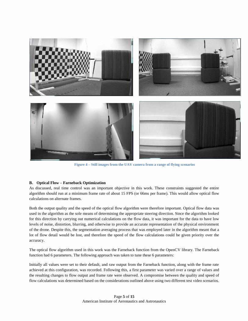
A. Data Acquisition & Simulation Videos from ARDrone flights were captured to be used to simulate the algorithm performance. Flight videos were recorded from the drone forward facing camera in small flying room. Textured cubical blocks were used to simulate obstacles. The test flights involved a range of flight scenarios and at a range of altitudes and speeds, both with and without a fisheye lens adapter attached to the drone camera. Flights involving direct collisions were also recorded. All calculations were run on a laptop computer running a 2.2GHz Intel Core2 Duo processor.

Figure 3 – 16 x 12 segmentation


B. Optical Flow – Farneback Optimization As discussed, real time control was an important objective in this work. These constraints suggested the entire algorithm should run at a minimum frame rate of about 15 FPS (or 66ms per frame). This would allow optical flow calculations on alternate frames.

Both the output quality and the speed of the optical flow algorithm were therefore important. Optical flow data was used in the algorithm as the sole means of determining the appropriate steering direction. Since the algorithm looked for this direction by carrying out numerical calculations on the flow data, it was important for the data to have low levels of noise, distortion, blurring, and otherwise to provide an accurate representation of the physical environment of the drone. Despite this, the segmentation averaging process that was employed later in the algorithm meant that a lot of flow detail would be lost, and therefore the speed of the flow calculations could be given priority over the accuracy.

The optical flow algorithm used in this work was the Farneback function from the OpenCV library. The Farneback function had 6 parameters. The following approach was taken to tune these 6 parameters:

Initially all values were set to their default, and raw output from the Farneback function, along with the frame rate achieved at this configuration, was recorded. Following this, a first parameter was varied over a range of values and the resulting changes to flow output and frame rate were observed. A compromise between the quality and speed of flow calculations was determined based on the considerations outlined above using two different test video scenarios.

Figure 4 – Still images from the UAV camera from a range of flying scenarios


Once this value had been determined it was set as the new default. This process continued for the 5 remaining parameters until all had been tuned to a new value.

To illustrate this process, data is presented from the 14th frame of a sample video of the drone flying towards a fixed obstacle. The figures show the raw flow output after each successive parameter had been set to its new value. Two parameters had no noticeable effect on the flow data output and are therefore not shown in the figure. In the greyscale raw flow data, areas of high optical flow magnitude are depicted by lighter areas and areas of low flow magnitude by darker areas. The frame rate was calculated as the average for the 13 preceding frames in the sequence and is shown in figure 5.

Parameter Changed Frame Rate (FPS) All default values 5.3 Pyramid Scale 7.1 Pyramid Layers 7.1 Averaging Window Size 7.1 Iterations per Level 9.4 Pixel Neighborhood Size 10.4 Gaussian Standard Deviation 10.4

Figure 5 – Table showing frame rate after each tuning stage


Figures 5 and 6 show the impact of successively tuning each parameter on the optical flow output. The flow output after optimization showed a small increase in noise levels and a small decrease in blurring when compared to the default, alongside a significant increase in speed. The final flow data was of suitable quality to clearly determine the outlines of obstacles and other structural features present in the original image. This was accompanied by a 96% increase in speed, giving a final frame rate of 10.4 FPS. While this rate was still below the goal of 15 FPS, it should be noted that the calculations were executed on a laptop computer with a slow processor and without hardware acceleration. The ground station PC used for controlling the drone was equipped with a faster processor and a graphics card, which would allow OpenCV to utilize hardware acceleration and shift much of the calculation to the graphics

Figure 6 - Compound image showing optical flow output after each parameter optimization. Top left is original camera image, top right after pyramid scale, middle left after window size, middle right after iterations, bottom left after size of pixel neighborhood, and

bottom right final result after poly sigma


card, significantly increasing performance. It is fully expected that these factors would provide an increase in speed enough to achieve the desired frame rate of 15 FPS.

C. Segmentation As outlined in the methods section, optical flow data was split into segments to represent potential steering directions. The size and shape of the segments was expected to have a large impact on the performance of the algorithm. The segmented flow data needed to retain sufficient information about the structure of the drone environment, but also to divide the flow into gaps large enough for the drone to fly through. In addition, increasing the number of segments would increase the number of splitting and averaging calculations the algorithm was required to perform on each video frame, reducing the frame rate and the possibility of real time control.

The composite figures 7, 8 and 9 show the algorithm output for increasingly fine uniform segmentation. Frames from three different flying scenarios were used in order to simulate the effect over a range of data. Scenario 1 involved an approach passing a single obstacle, scenario 2 involved an approach between two obstacles and scenario 3 involved a flight past a group of obstacles with the use of a fish-eye lens adapter.

The results highlighted that in order to recover a similar level of detail contained within the original flow data, a relatively fine segmentation approach was needed. For the example frames shown, this level of detail was reached with flow segmentation approximately 64 segments wide and 32 segments high (64 x 32). This result is unsurprising since the flow segments were effectively being viewed like image pixels; increasing the number of ‘pixels’ gave a higher image resolution. More unexpected was the amount of useful information that could be observed with a coarsely segmented flow. In figures 7 and 8, the 4x2 and 8x4 segmentations both show clear dark regions in the direction of gaps that would have represented good steering choices. The flow data in figure 9 from the fish-eye adapter shows a less detailed overall view, with gap regions not as clearly differentiable as with the standard lens.

The calculation time to segment the optical flow data increased roughly linearly with the number of segments making up the flow. Importantly, the timing data showed that the algorithm could segment the optical flow data very quickly. A 16x8 segmentation could be carried out in 4.4 milliseconds, which is over 20 times quicker than the time taken to calculate the optical flow, which took 96 milliseconds as optimized previously.


Figure 9 – Segmented flow output for Test Scenario 2. Segmentations 4x2, 8,4, 16x8, 32x16, 64x32 and 128x64 shown.

Figure 8 – Segmented flow output for Test Scenario 2. Segmentations 4x2, 8,4, 16x8, 32x16, 64x32 and 128x64 shown.

Figure 7 – Segmented flow output for Test Scenario 1. Segmentations 4x2,

8x4, 16x8, 32x16, 64x32, 128x64 shown


D. Gap-finding Simulations The final stage of the algorithm used the segmented optical flow data to determine the drone steering direction. This was achieved by identifying the location of the column of segments with the lowest optical flow magnitude and representing it as a steering angle in degrees. The ability of the algorithm to accurately and reliably identify the gap direction was heavily influenced by the size of segments used, which is the focus of the first part of this section. Additionally, the steering output generated from this process was very unsteady, since switching between flow columns generated step changes in the steering output.

Simulations in this section were conducted with two test videos. Video 1 involved the drone flying towards a single obstacle just to the right of center, while video 2 involved a flight passing between two obstacles. Figure 10 shows a still from test video 1 indicating the axis system used in the simulations. The lens field of view was 68 degrees, and the origin was located at the geometric image center.

In order to simulate the gap direction, for each frame in a video the left and right edges of the gap were identified visually and converted into an angle in degrees. In the following figures the left and right edges of the main gap (there may have been more than one present) as viewed from the drone camera are plotted as dashed blue and red lines respectively.

Timing data is not presented for the gap finding section of the algorithm because all operations took <1ms.

Segmentation The algorithm identified a steering direction by evaluating the segment region with the lowest optical flow. Simulations for a range of segmentation approaches showed the steering direction gave a very unsteady output. The output oscillated over the gap direction and also showed a tendency to switch between gaps if more than one was present. Coarser segmentation gave a lower mean steering error, but also more abrupt changes in steering direction and less range. A 4x2 segmentation was identified as giving a good compromise between these factors.

Moving Average The steering output was smoothed using a moving average. Simulations showed the introduction of the moving average reduced the mean error and smoothed the oscillations that were present in the original output. Simulations were used to investigate the effect of increasing the number of frames included in the moving average on the steering output. Figure 11 shows the steering angle against time in relation to the actual gap direction (dashed line) with a

Figure 10 – Simulation axis system


different number of frames included in the moving average. It was found that the optimum level varied with different scenarios, but including around 60 frames gave good behavior in both simulation cases, as can be seen from figure 12.

VI. Results

-34.0

-30.0

-26.0

-22.0

-18.0

-14.0

-10.0

-6.0

-2.0

2.0

6.0

10.0

14.0

18.0

22.0

26.0

30.0

34.0

0.00 2.00 4.00 6.00 8.00 10.00 12.00

An

gle

(d

eg

ree

s)

Time (secs)

Left Edge Right Edge 10 30 60

0

5

10

15

20

25

0 20 40 60 80 100

Me

an

Err

or

(de

gre

es)

Moving Average Frames

Figure 11 - Graph showing algorithm output against time with different moving averages for scenario 1. Visual gap direction is shown for comparison

Figure 12 - Graph showing simulation mean error against number of moving average frames for two test scenarios. Scenario 1 is shown in blue and scenario 2 is shown in red


This section outlines the algorithm performance after the optimisation detailed in the previous section.

The final algorithm performance was evaluated using simulation videos that were different from those used in the optimization process described previously. Two video scenarios were chosen because they presented a challenging object avoidance problem. Scenario 3 (figure 13) involved flying the drone through the center of a very narrow gap. Scenario 4 (figure 14) involved flying the drone towards an obstacle then making a sharp right turn to avoid it, before steering left again through another gap. The results were obtained using a 4x2 segmentation and with a 60 frame moving average.

Figure 13 – Algorithm steering output compared with visual gap direction for narrow gap navigation scenario

The results of video 3 shows the algorithm steering output when travelling through a narrow gap (figure 13) At the beginning of the simulation, the gap represented about 10 degrees of the drone field of view. The steering output remained within the gap direction for the majority of the simulation and showed a low mean error of 3 degrees. At approximately 5 seconds, the steering output was observed to diverge towards the left edge of the gap. This was followed by a strong steering direction in the opposite direction, before the output returned to the gap center. Despite this behavior, the short period of the divergence and the nature of the compensatory motion mean that it is probable that the drone would have navigated successfully through the gap presented in this simulation.

-34.0

-30.0

-26.0

-22.0

-18.0

-14.0

-10.0

-6.0

-2.0

2.0

6.0

10.0

14.0

18.0

22.0

26.0

30.0

34.0

0.00 2.00 4.00 6.00 8.00 10.00 12.00

An

gle

(d

eg

ree

s)

Time (secs)

Left Edge Right Edge Algorithm Output


The simulation on video 4 (figure 14) shows the algorithm performance in a challenging scenario. The steering output demonstrated two discrete periods of divergence, occurring at 6 and 10 seconds, which were followed by an over-compensatory movement in the opposite direction. This behavior resulted in a high value of mean error of 12 degrees from the gap center. While the algorithm steering commands did coincide with the general gap direction, the two divergent behaviors mean that it is questionable whether the drone would have successfully navigated the field of obstacles in this simulation. A longer moving average might have reduced the divergent tendency, although it would also have slowed the response speed.

VII. Conclusion

This work has demonstrated a novel biomimetic algorithm for use with UAV obstacle avoidance. By simplifying the control problem down to yaw control, a simple algorithm was able to be used to simulate obstacle avoidance in a range of flying scenarios. The main benefit of the approach highlighted in this work - using optical flow in conjunction with a simple control algorithm - is that it does not require a lot of sensing or computing power. This makes it particularly suitable for use with small, lightweight UAVs. While some promising results were obtained in the simple simulations outlined, testing the performance of the algorithm using more rigorous simulation techniques and ultimately with a real flying scenario is important before firm conclusions can be reached.

Contrary to the assumptions of a lot of existing optical flow research, this work shows that the quality of optical flow data generated from camera motion through an environment is relatively insensitive to the camera motion. The range of translatory and rotational movement that naturally arise from the motion of a camera attached to a moving vehicle produce optical flow output with a consistently high level of structural detail. A limiting factor in a lot of previous work has been the weight and power requirements of the microprocessors and sensors that were needed, but the current research shows that lightweight approaches have the potential to fulfill the wider goals of the field. Taken together, these findings suggest an alternative approach to developing autonomous vehicles that can yield better progress.

-34

-30

-26

-22

-18

-14

-10

-6

-2

2

6

10

14

18

22

26

30

34

0.00 2.00 4.00 6.00 8.00 10.00 12.00 14.00

An

gle

(d

eg

ree

s)

Time (secs)

Left Edge Right Edge Algorithm Output

Figure 14 – Algorithm steering output compared with visual gap direction for alternative scenario


Rather than becoming preoccupied by the quest to capture ever more accurate data, we should take inspiration from nature by finding better ways of using the data we already have.

Acknowledgments

The research was partially supported by the EPSRC Green Brain Project (grant number EP/J019690/1). The author would also like to acknowledge J. R. Marshall for their help in this work.

References

[1] S. Gupte, P. Mohandas and J. M. Conrad, "A Survey of Quadrotor Unmanned Aerial Vehicles," in Southeastcon, 2012 Proceedings of IEEE, Orlando, FL, 2012.

[2] B. P. Tice, "Unmanned Aerial Vehicles - The Force Multiplier of the 1990s," Airpower Journal, no. Spring 1991, 1991.

[3] S. Ackerman and N. Shachtman, "Almost 1 In 3 U.S. Warplanes Is a Robot," 9 January 2012. [Online]. Available: http://www.wired.com/2012/01/drone-report/. [Accessed 2 December 2014].

[4] M. Srinivasan, "Honeybees as a Model for the Study of Visually Guided Flight, Navigation, and Biologically Inspired Robotics," Physiological Reviews, vol. 91, pp. 413-460, 2011.

[5] N. Franceschini, "Small Brains, SmartMachines: From Fly Vision to Robot Vision and Back Again," Proceedings of The IEEE, vol. 102, 2014.

[6] C. Goerzen, Z. Kong and B. Mettler, "A Survey of Motion Planning Algorithms from the Perspective of Autonomous UAV Guidance," J Intell Robot Syst, vol. 100, pp. 57-65, 2010.

[7] A. Beyeler, J.-C. Zufferey and D. Floreano, "Vision-based control of near-obstacle flight," Auton Robot, no. 27, pp. 201-219, 2009.

[8] Y.-c. Liu and Q.-h. Dai, "Vision Aided Unmanned Aerial Vehicle Autonomy: An Overview," in 3rd International Congress on Image and Signal Processing, Yantai, China, 2010.

[9] S. Ross, N. Melik-Barkhudarov, K. Shaurya Shankar, A. Wendel, D. Dey, J. A. Bagnell and M. Hebert, "Learning Monocular Reactive UAV Control in Cluttered Natural Environments," in IEEE International Conference on: Robotics and Automation, Karlsruhe, 2012.

[10] P. Bhagavatula, C. Claudianos, M. Ibbotson and M. Srinivasan, "Optic Flow Cues Guide Flight in Birds," Current Biology, vol. 21, pp. 1794-1799, 2011.

[11] A. Schwegmann, "Depth information in natural environments derived from optic flow by insect motion detection system a model analysis".

[12] H.-T. Lin, I. Ros and A. Biewener, "Through the eyes of a bird: modelling visually guided obstacle flight," J R Soc Interface, vol. 11, 2014.

[13] G. Bradski and A. Kaehler, "Optic Flow," in Learning OpenCV, Sebastopol, O'Reilly Media, 2008, pp. 322-337.


[14] G. Farneback, "Two-Frame Motion Estimation Based on Polynomial Expansion," Lecture Notes in Computer Science, vol. 2749, pp. 363-370, 2003.

[15] O. Merry, "Using Optic Flow for Navigation of an Autonomous Quadcopter," University of Sheffield, Sheffield, 2014.

[16] G. B. Project, "About the project," 2015. [Online]. Available: http://greenbrain.group.shef.ac.uk/. [Accessed 02 05 2015].

[17] Parrot, "Parrot ARDrone 2.0 - User Guide," 2013. [Online]. Available: http://parrotcontact.emencia.net/website/user-guides/download-user-guides.php?pdf=ar-drone-2/AR-Drone-2_User-guide_Android_UK.pdf. [Accessed 02 05 2015].

[18] OpenCV Developer Team, "About," 2015. [Online]. Available: http://opencv.org/about.html. [Accessed 01 05 2015].

quadcopter obstacle avoidance using biomimetic algorithmseprints.whiterose.ac.uk/96477/1/as of obs...

Documents