qp - ad&co · pdf fileqp. introduction the andrew davidson ... the model incorporates the...

Quantitative PerspectivesMay 2006

Fixed-Rate Agency MBS Prepayments &Model Enhancements

by Dan Szakallas

QP

Introduction

The Andrew Davidson & Co., Inc. Fixed Rate Prepayment Model version 5.1 represents a major step

forward in prepayment modeling. The model incorporates the Active-Passive Methodology for

burnout as well as the enhanced pool data from Fannie Mae, Freddie Mac and Ginnie Mae. This

model is based upon pool data from 1992 to 2005 and the enhanced data disclosure from the

agencies beginning in June 2003. The initial version of the model was released in October 2005.

This article begins with a discussion of our prepayment modeling philosophy. Next, we explain the

data and the existing factors in our model. We review, in detail, the various factors that drive the

model and discuss a new approach to modeling the 'burnout' effect seen in prepayment modeling.

We will comprehensively examine this approach, called Active-Passive Decomposition (APD), and

illustrate its advantages for modeling and for valuation purposes. We will also discuss how the

Agency data disclosures are incorporated into the new Enhanced Prepayment Model. Finally, we will

compare prepayment model output from v5.1 to the previous version of the pool model and review

valuation results using our OAS and interest rate routines and the new prepayment model.

Andrew Davidson & Co., Inc. (ADCo) believes that prepayment modeling at the pool level is a

mixture of science and art. The key components of prepayments have been understood and

modeled for some time, and a variety of statistical techniques exist to model many of the non-linear

features of prepayment behavior, such as interest rate effects and housing turnover. The various

factors affecting prepayments, however, tend to interact in ways in which standard statistical

techniques may be ill-equipped to handle. Borrower behavior changes over time due to structural

changes in the market, and new factors may influence when and why prepayments occur. For

example, in our last model release, we examined how home price appreciation began to spur the

'cash-out' refinance--in which borrowers were refinancing their loans in order take advantage of the

equity in their homes.1 This was a notable addition because it helped explain higher prepayments

during periods when no real interest rate incentive was apparent. Furthermore, many of the

forecasts that a good model will have to generate for stress-testing and OAS will be for combinations

of factors that have not previously had significant impact on prepayments.

Our modeling approach emphasizes simplicity, robustness and efficiency while recognizing the

importance of both historical model fit and forecasting ability. In the past, we tended to re-fit the

model every 18 to 24 months and add additional factors only after determining their longevity in

affecting future prepayments and gathering sufficient evidence to warrant their introduction. This

latest version, rather than just a re-fit of parameters to more recent data, is a completely new

model. We changed the way certain model features are implemented and introduced new

characteristics that accurately capture unfamiliiar borrower behavior.

Quantitative Perspectives May 2006

Modeling Philosophy

1 See "Home Price & Prepayments: The New Andrew Davidson & Co., Inc. Prepayment Model", Quantitative Perspectives, July2001.

In addition to using historical data to fit model parameters, we adjusted the models to perform

reasonably well across a wide-variety of stress tests and scenarios never experienced in history. As a

supplement to these assessments, we evaluated the impact of changing prepayment model

parameters under a variety of interest rate scenarios on valuation and risk measures such as OAS,

effective duration and convexity.

To estimate the Fixed-Rate MBS Pool Level Prepayment Model, we used pool-level prepayment data

with the following variables:

- Weighted Average Loan Age (WALA)

- Weighted average gross coupon (GWAC)

- Current Balance

- Origination year

- Origination quarter

- One-month prepayment speed

For the Enhanced Pool Level Model, we considered these additional factors:

- Average Original Loan Balance

- Weighted Average Original LTV

- Weighted Average Original Credit Score (FICO)

- % of refinanced loans in pool

- % of new purchase loans in pool

- % of single-family loans in pool

- % of multi-family loans in pool

- % of owner loans in pool

- % of second homes in pool

- % of investment properties in pool

- % geographical composition of pool

This data covers Agency pools originated in 1991 going forward to originations through the third

quarter of 2005. We have monthly prepayment data for all pools through August 2005, and we used

the history for additional enhanced pool data from June 2003 through December 2004.

In addition to pool performance data, we applied monthly mortgage current coupon data (the rate at

which mortgages trade at par) and interest rate data (treasuries, LIBOR, etc.) from Bloomberg and

home price index data provided by Mortgage Risk Assessment Corporation (MRAC). MRAC's home

price appreciation indices (HPI) is calculated using a repeat sales methodology on a monthly sales

database of approximately 52 million properties.


Page2

The Data


The main factors in the fixed rate MBS pool model are turnover, refinance incentive, cash-out

(home price appreciation) and credit cure. Within these factors, other effects such as aging,

seasonality, spread at origination (SATO) and yield curve spread (basis point spread between

the two and 10 year LIBOR rates) are used as well. We will explore why these factors are

important elements of the pool-level prepayment model and then discuss the concepts of aging

and burnout.

Turnover & Seasonality

In the absence of a refinancing incentive, one of the main drivers of prepayments is natural

housing turnover. Natural housing turnover occurs for reasons like change in employment

status or location, change in family size, divorce, etc. It tends to be seasonal in nature and

depends on the age of the loan. For example, a greater proportion of people are inclined to

move in the summer, and most people have a propensity to not sell their home within 12

months of obtaining their mortgage because of various costs involved. Turnover is heavily age

dependent, and we will discuss how aging impacts prepayments shortly.

The seasonality component of turnover captures the cyclical trend in which turnover increases

in the late spring and summer months and diminishes during the fall and winter months as

demonstrated in Figure 1. This pattern has many causes, though weather and the school year

are the standouts. People are less likely to move during the cold winter months and during the

time when their children are in school.

Page3

Model Factors

0.6

0.8

1.0

1.2

1.4

Jan Feb Mar Apr May Jun Jul Aug Sep Oct Nov Dec

Month

Seas

onal

ity M

ultip

lier

Figure 1


Page4

Refinance Incentive

By far, the most important factor that drives fixed-rate MBS prepayments is the level of current

mortgage rates as defined by the current coupon yield plus a spread relative to the weighted-average

gross coupon (GWAC) on the pool of mortgages. If a borrower has a higher interest rate than what is

currently available in the market, the borrower will tend to refinance into the lower market rates,

causing the prepayment speed of that pool to increase. The larger the difference between the rate

held by the borrowers in the pool and the current market rate reference, the faster prepayment speeds

become.

We aim to capture the change in a borrower's monthly mortgage payments rather than just the change

in mortgage rates. Within the model, we calculate an incentive that takes into account several factors:

the GWAC of the pool

the remaining time to maturity of the pool

the difference between the coupon on the pool and the prevailing market coupon at the

time it was originated

the difference between the two-year and ten-year LIBOR rates

We also add a spread to the market reference rate to accurately compare it to the gross coupon. This

spread is calculated by looking at the average difference between the pass-through rate and the gross

rate on pools of each collateral type. For the market reference rate, we weight and sum the last three

months of mortgage current coupon rates; the exact weights are based on historical data.2 The reason

we use lagged rates is that there is a slight delay between drops in rates and increased refinancing,

although this delay is shrinking over time. Five years ago, the weightings were more evenly dispersed

over the three month time period, but recently we have seen a shift to the prior two months with much

less weight being placed on the third month. It currently takes less time from the start of the

refinance process to completion than ever before.

We examine the difference between the original GWAC and the market reference rate at origination in

order to determine what we call spread at origination (SATO). In the basic pool model, we do not

know the credit score (FICO) of the pool, so we use SATO as an approximation (we discuss the use of

FICO in the Enhanced Model later). If this number is large, it means the pool is made up of loans that

had some type of constraint that prevented them from being originated at the lower prevailing rate.

This could be due to poor credit, not enough documentation or some other factor. Whatever the case,

these types of pools behave differently because of this feature, so the model uses this information

when determining the refinance incentive for the pool.

The Yield Curve Spread Effect

A feature added to this version of the Pool Model is the incorporation of the difference between the

2 For more about mortgage current coupons and their dynamics relative to Treasury or Libor/Swap rates, see "The RelationshipBetween the Yield Curve & Mortgage Current Coupon," Quantitative Perspectives, April, 2001


Page5

2 year and 10 year LIBOR rates, termed the "Yield Curve Spread Effect." This spread provides

valuable insight as to whether refinancing out of a fixed-rate mortgage into an adjustable-rate

mortgage (ARM) would be beneficial to the borrower. When the spread between the two rates is

large, it tells us that the yield curve is steep and that the short term rate is significantly less than the

long term rate. Since interest rates for ARMs are based on the short term rates, the borrower would

be able to lower their monthly payment by refinancing their fixed-rate 30 year mortgage into an ARM.

This provides a refinance incentive even when the GWAC of the pool and the market reference rate

are nearly equal. Conversely, when the spread between the 2 year and 10 year rate is small, there is

no real payment incentive for the borrower to refinance into an ARM, so the overall refinance

incentive is dampened. With the explosion of the hybrid and option ARM market over the last few

years, we felt the Yield Curve Spread Effect a necessary addition to the model because it helps

explain why prepayment speeds change during a perceived stable mortgage rate environment.

Now that we have considered many of the characteristics that comprise refinance incentive, let's look

at an example. Figure 2 displays a sample refinancing incentive curve. As the calculated refinance

incentive discussed above increases past 1.0, refinancing begins to pick up significantly and then

levels off after peaking. A good way to understand this graph is to think of the portion below 1.0 as

representative of loans with interest rates below the current market rate, and the portion above 1.1

to represent those with interest rates above the current market rate. The higher the incentive, the

more likely prepayment will occur.

The S-shaped curve in Figure 2 is a composite based on a variety of borrowers living in different

states who face different sets of financial and non-financial costs. In addition, some borrowers pay

greater attention to the level of rates than others. As interest rates drop, the more aggressive

refinancers tend to leave the pool first, effectively changing the shape of the curve as they exit. We

will discuss how this change in the pool composition is captured when we discuss burnout later in this

paper.

0.00

0.05

0.10

0.15

0.8 1.0 1.2 1.4 1.6

Ratio

SM

M

Prepayment Speed

Figure 2

Refinance Incentive


The Home Price (Cash-out) Effect

We introduced the Home Price Appreciation Effect into the Pool Model in 2001. In the late 1990's

and through the end of 2000, we witnessed a steady increase in the appreciation of home values

over time. With equity building up in their homes, borrowers were re-financing their mortgages to

take advantage of this inexpensive source of money. Through "cash-out refi," borrowers were

essentially going through the refinance process in order to access the equity built up in their homes.

This factor is based on a national home price appreciation index, and we look at the change in the

index from a loan's origination forward for a maximum to 24 months, and from then on we look at

the two year change.

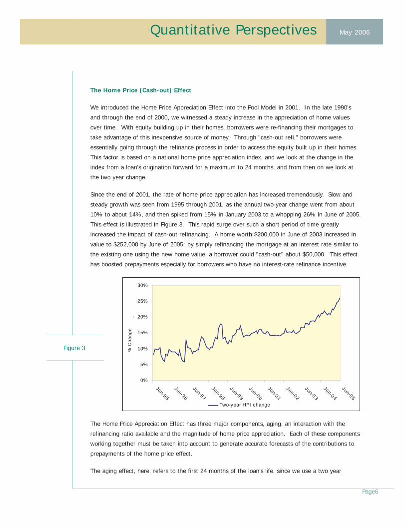
Since the end of 2001, the rate of home price appreciation has increased tremendously. Slow and

steady growth was seen from 1995 through 2001, as the annual two-year change went from about

10% to about 14%, and then spiked from 15% in January 2003 to a whopping 26% in June of 2005.

This effect is illustrated in Figure 3. This rapid surge over such a short period of time greatly

increased the impact of cash-out refinancing. A home worth $200,000 in June of 2003 increased in

value to $252,000 by June of 2005: by simply refinancing the mortgage at an interest rate similar to

the existing one using the new home value, a borrower could "cash-out" about $50,000. This effect

has boosted prepayments especially for borrowers who have no interest-rate refinance incentive.

The Home Price Appreciation Effect has three major components, aging, an interaction with the

refinancing ratio available and the magnitude of home price appreciation. Each of these components

working together must be taken into account to generate accurate forecasts of the contributions to

prepayments of the home price effect.

The aging effect, here, refers to the first 24 months of the loan's life, since we use a two year

Figure 3

Page6

0%

5%

10%

15%

20%

25%

30%

Jun-95

Jun-96

Jun-97

Jun-98

Jun-99

Jun-00

Jun-01

Jun-02

Jun-03

Jun-04

Jun-05

Per

cent

Cha

nge

Two-year HPI change

% C

hang

e


change in HPI as our incentive driver. During the first 24 months in the life of a pool, the incentive is

calculated using the change in the home's value since loan origination. After the 24th month, the

incentive is calculated using the change from the current month and 24 months prior. For example,

for a loan with an age of 48 months in February 2005, the calculated HPI incentive would be relative

to February 2003. Going forward, the model's HPI forecast is, in essence, a rolling two years.

Next, borrowers are less likely to take equity out when the cost of doing so is a higher new mortgage

rate. Hence, the ratio of the current loan to prevailing market rates is an important determinant of

cash-out refinancing. Moreover, as that ratio becomes more favorable to the borrower, purely rate-

based motives take over, and the marginal effect of home price appreciation past a certain ratio

should be minimal.

Credit Cure Effect

The last key factor in this version of the pool-level prepayment model is what we have termed the

Credit Cure Effect. As discussed in the Refinance Incentive section, borrowers sometimes have less

than pristine credit and, as a result, may be forced to borrow at a rate that is measurably higher than

the prevailing market rate. As these borrowers make several consecutive on-time payments, their

credit will improve, making them eligible to receive a prime-based rate if they refinance. Once this

happens, these borrowers will refinance their loans, creating an increase in prepayment speeds even

though mortgage rates may have remained constant for a given period. To capture this effect, we

look at the spread between the rate on the loan and the prevailing market rate at the time the loan

was originated (SATO). The greater the spread, the greater the likelihood of a refinance occurring

after credit improves.

This effect is based on both an aging component and the SATO component. As the loan age

increases and there are no missed payments, the ability of the borrower to refinance increases; so

the effect becomes stronger, contributing more to the overall prepayment speed. The SATO has an

impact on this effect as well, with prepayment speed increasing along with the SATO.

Now that we have gone over the primary model effects (except for the vintage-based loan size effect,

which will be discussed later in the paper), we'll look at how they interact with one another and how

we model burnout. Our modeling of burnout is the part of the model that has changed most

significantly from previous versions, and it represents the basis for all ADCo prepayment models

going forward.

Our new approach to burnout modeling is a concept introduced by Alex Levin et al.3 The APD

method of modeling burnout is unique in that it treats a single pool of loans as essentially two

Page7

Active-Passive Decomposition

3 See "Divide and Conquer: Exploring New OAS Horizons", Quantitative Perspectives, September 2003-June 2004.


Page8

pools — one of "active" borrowers and one of "passive" borrowers. The assumption is that the

active borrowers are more sensitive to refinance opportunities and are aware of market conditions

pertaining to mortgage interest rates. These borrowers are likely to prepay to take advantage of a

lower interest rate, a more favorable loan type or to cash out on the equity built up in their home.

The other pool consists of the passive borrowers who are much less sensitive to refinance

opportunities. The pool consisting of passive borrowers experiences prepayments mostly as a result

of turnover. Passive borrowers, for whatever reason, do not respond to favorable refinance

scenarios, even when they could save thousands of dollars. They do experience a small amount of

refinance incentive, but not nearly as much as their active counterparts. We will discuss this in

further detail later in the paper. It is this group that usually causes the burnout seen in seasoned

MBS pools.

The key to APD is the ability to accurately identify the breakdown of active and passive borrowers

for a given MBS pool without knowing actual pool composition, that is, without having exact

characteristics of each loan in the pool. In this identification, it is important to assume no migration

between the active and passive borrowers within a given pool. A borrower cannot be passive at the

origination of the pool and then later become an active borrower. It is this strict classification of two

distinct pools that allows the APD method to function.

There are several concepts that enable APD to accurately model burnout of an MBS pool. The first

notion is the breakdown of the pool into its two components as we just discussed. The key

compositional variable is designated by Ψ, where Ψ represents the percent of active borrowers in

the pool, and 1 - Ψ represents the percent of passive borrowers in the same pool. When the pool is

first created, Ψ0 represents the initial percentage of active borrowers within the given pool. This Ψ0is estimated when building a prepayment model, and Ψ0 can differ among collateral types. The

overall prepayment speed depends on this active-passive split going forward, and Ψ decreases over

time as the active borrowers leave the pool.

We discussed the main prepayment model factors earlier, and now we will examine how they

interact with each other to forecast prepayments. To compute the total prepayment speed in single

monthly mortality rate (SMM), APD computes an SMM for the passive piece and an SMM for the

active piece. Below is the calculation for the active piece with refi, turnover, cash-out and cure as

components of the prepay model:

ActiveSMM = turnoverSMM + refiSMM + cash-outSMM + cureSMM (Eq. 1)

Active-Passive Decomposition Mathematics


As mentioned in the introduction to APD, the passive piece does experience some refinance

incentive, but not on the same level as the active piece. The calculation for the passive piece is as

follows:

PassiveSMM = turnoverSMM + β1*refiSMM + β2*cash-outSMM + β3*cureSMM (Eq. 2)

In this expression, the different betas represent the amount of each SMM relative to the SMMs from

the active piece. These values are typically 25% or less. Also, it is important to note that the

passive turnoverSMM does not have a beta associated with it because turnover is the same for both

the active and passive pieces of APD, and because turnover itself is an effect that is almost

independent of interest rates. The next step is to compute the total SMM for the entire pool. This

is done as follows:

TotalSMM = Ψ* activeSMM + (1 - Ψ) * passiveSMM (Eq. 3)

Now that we have demonstrated how to compute the monthly SMM from the active and passive

subpools, it is time to investigate how Ψ decreases over time. To calculate Ψ for the next month,

we use the following formula, where k represents the age in months of the pool:

Ψk+1 =Ψk * {(1-ActiveSMMk) / (1-TotalSMMk)} (Eq. 4)

As active borrowers refinance and leave the pool, the ratio of activeSMM to totalSMM decreases and

thusly Ψ decreases. Tracking Ψ over time is a good way to judge how burnt out a given pool is. If

Ψ is around 60%, the pool still has significant refinancibility. If Ψ is around 15%, the pool is very

burnt out, i.e. made up mostly of passive borrowers.

The following exhibits help illustrate how APD works. Figure 4 shows what a typical MBS pool's

prepayments will be when broken down into the active and passive sub-pools. It is easy to see that

the active piece's prepayment speed is heavily weighted toward the refinance component of the

prepayment model, while the passive portion's prepayment speed is more equally weighted between

the refinance and turnover components. Two things are important to note from Figure 4. First,

turnover is the same in both the active and passive sub-pools. As discussed in the previous section,

the TurnoverSMM in Eq. 2 does not have a beta scalar associated with it because turnover is a basic

component of prepayments and, therefore, is a part of both the active and passive sub-pools.

Second, the refinance component of the passive piece is scaled in relation to the refinance

component of the active piece. If we say that turnover accounts for 8 CPR in both the active and

Page9

Active-Passive Decomposition in Practice


passive sub-pools, then we see that the 9 CPR refinance component of the passive piece is 15% of the

60 CPR refinance component of the active piece. That 15% is the value of β from Eq. 2 from the

previous section.

Figure 4 illustrates the mix of the refinance and turnover components of APD, and now we will look at

a graph that demonstrates the decrease of Ψ over time. The following two charts in Figure 5 represent

the same MBS pool from Figure 4, but at different ages. In this example, let's assume that the

ActiveSMM (in CPR) is 68 CPR and the PassiveSMM is 17 CPR. At origination, we see that Ψ0 is 80%

and that active borrowers make up most of the pool. As the pool ages, active borrowers refinance and

leave the pool, thereby, diminishing the impact of Ψ on the overall prepayment speed. Looking at the

same pool after it has aged, we can see that most active borrowers have left the pool, and only 27%

of the pool is made up of active borrowers. Even though those active borrowers are prepaying at 68

CPR, the overall pool speed is only 31 CPR because the pool is more heavily weighted toward the

passive borrowers.

0

10

20

30

40

50

60

70

80

Active Passive

Prep

aym

ent R

ate

(CPR

)

RefinancingTurnover

ActivePassive

Figure 4

Page10

ActivePassive

Prepayment speed (0.80*68 + 0.20*17) = 58 Prepayment speed (0.27*68 + 0.73*17) = 31

Figure 5


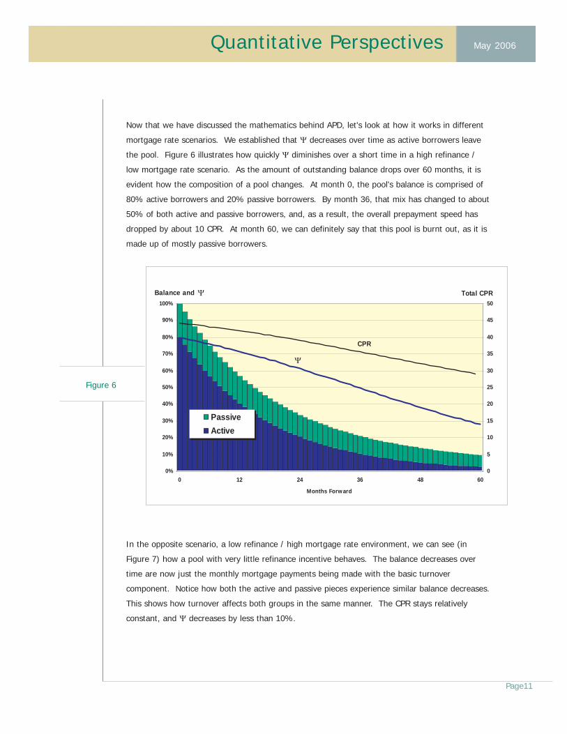
Now that we have discussed the mathematics behind APD, let's look at how it works in different

mortgage rate scenarios. We established that Ψ decreases over time as active borrowers leave

the pool. Figure 6 illustrates how quickly Ψ diminishes over a short time in a high refinance /

low mortgage rate scenario. As the amount of outstanding balance drops over 60 months, it is

evident how the composition of a pool changes. At month 0, the pool's balance is comprised of

80% active borrowers and 20% passive borrowers. By month 36, that mix has changed to about

50% of both active and passive borrowers, and, as a result, the overall prepayment speed has

dropped by about 10 CPR. At month 60, we can definitely say that this pool is burnt out, as it is

made up of mostly passive borrowers.

In the opposite scenario, a low refinance / high mortgage rate environment, we can see (in

Figure 7) how a pool with very little refinance incentive behaves. The balance decreases over

time are now just the monthly mortgage payments being made with the basic turnover

component. Notice how both the active and passive pieces experience similar balance decreases.

This shows how turnover affects both groups in the same manner. The CPR stays relatively

constant, and Ψ decreases by less than 10%.

Page11

0%

10%

20%

30%

40%

50%

60%

70%

80%

90%

100%

0 12 24 36 48 60

Months Forw ard

Balance and PSI

0

5

10

15

20

25

30

35

40

45

50Total CPR

PassiveActive

PSI

CPR

Figure 6

Ψ

Ψ


The APD model naturally simulates the burnout and other prepayment effects, such as incentive-

dependent speed ramping or "catch-up" for prepay-penalty pools. We feel that this is an

improvement over previous methods of capturing burnout, not only because of model accuracy but

because it opens doors to new valuation and modeling tasks in combination with new enhanced

agency data disclosures. We will explore this further in the next section.

Introduction to Enhanced Agency Pool Data

In June 2003, both Fannie Mae and Freddie Mac began to release more pool-level data, which they

referred to as the enhanced data disclosures. This additional data can be used to estimate more

accurate prepayment models, and it allows analysts to value specific pools versus TBA's, in which the

only information available is the mortgage coupon, weighted average loan age (WALA) and collateral

type. We will examine these new data fields and explain why each is important to prepay modeling.

Enhanced Data

Six different data elements were made available in June 2003:

- Weighted-Average Original LTV

- Weighted Average Original FICO Score

- Loan Purpose

- Occupancy Type

- Property Type

0%

10%

20%

30%

40%

50%

60%

70%

80%

90%

100%

0 12 24 36 48 60

Months Forward

Balance and PSI

13.0

13.5

14.0

14.5

15.0

15.5Total CPR

PassiveActive

PSI

CPR

Enhanced Agency Data

Figure 7

Page12

Ψ

Ψ

These data elements plus Weighted-Average Original Loan Balance and Geographical Distribution, which

have been provided for some time, are given for each pool Freddie Mac and Fannie Mae have issued

for all collateral types.

Weighted-Average Original Loan Balance is the amount, in dollars, of the total original pool balance

divided by the number of loans in the pool. Weighted-Average Original LTV represents the average

loan-to-value ratio for the entire pool at origination. Loan-to-value is the ratio of the mortgage amount

to the actual value of the house. Weighted-Average Original FICO Score is the average credit score of

the entire pool at origination. Both Weighted-Average Original LTV and Weighted-Average Original

FICO score are balance-weighted values based on individual loan sizes in the pool.

The next four data elements contain categories, unlike the three we just described, that are

represented with one number. Loan Purpose contains two categories: Purchase or Refinance; referring

to whether the loan was for a new home purchase or a refinance of an existing mortgage. It is

reported using the amount of pool balance in each category, and the total number in each will sum to

the total pool balance. Occupancy Type has three categories: Owner, Second Home or Investment

Property. These are also reported using pool balance, and all three categories will sum to the total

balance of the pool. Property Type contains two categories: Single Family or 2 to 4 Family; referring to

the type of housing unit the loan represents. Like the previous two data elements, it also is reported in

pool balance and sums to the original balance of the pool. Finally, we have the Geographic Distribution

of each pool, which tells what amount of balance from the pool is comprised of loans from different

states. Adding up each state's balance will give you the original balance of the pool. Loan Servicer

disclosure is not included in our modeling effort because we prefer to utilize measures that relate

directly to the underlying loan.

It is helpful to examine these seven data elements in two groups. Weighted-Average Original Loan

Balance (WAOLB), Weighted-Average Original FICO (FICO), and Weighted-Average Original LTV

(WAOLTV) all fall into the same group, because they are reported as single discrete values, for example

$155,000 for WAOLB, 720 for FICO, and 80% for WAOLTV. The other three; Occupancy Type, Property

Type and Geographical Distribution fall into the same group because they are categorical and are best

represented as percents of original balance. For example, Loan Purpose has two categories; Purchase

or Refinance. These are best expressed in the manner of 90% Purchase, 10% Refinance for a given

pool. The same method applies to the other three elements in this group. Since these will all sum to

100%, we may use the data in this form for prepayment model estimation. Let's take a look at some

of the balance distributions for these new data elements.

Characteristics of Enhanced Data

We will look at the data for all Fannie Mae and Freddie Mac 30-year pools from June 2003 to December

2004 to get an idea of what an "average" pool might look like. We broke down WAOLB, FICO, and


Page13


WAOLTV into different buckets and examined the balance distribution in each. To produce the

following graphs, we examined what the overall outstanding balance was for pools that fell into each

of the classes and then calculated the percentage of each class relative to the overall outstanding

balance of the dataset. Figure 8 shows the breakdown for WAOLB.

Here we can see that the largest percent of balance falls in the $125,000 to $150,000 class. This

appears to be an approximately normal distribution with steady slopes outward from the midpoint.

Moving to FICO, Figure 9 displays the distribution among the different FICO classes.

Average Original Loan Balance

0%

5%

10%

15%

20%

25%

0K - 50K 50K -75K

75K -100K

100K -125K

125K -150K

150K -175K

175K -200K

200K -225K

225K -250K

>250K

Loan Balance

Perc

ent o

f Ove

rall

Average Original FICO

0%

10%

20%

30%

40%

50%

0 - 670 670 - 690 690 - 710 710 - 730 730 - 750 >750FICO Score

Perc

ent o

f Ove

rall

Page14

Figure 8

Figure 9


We see the same general distribution as in the previous graph, but with a definite skew to the right,

and with the 710 to 730 FICO class containing the largest percentage of original balance. Only

about 8% of the balance falls below 690, as it becomes increasingly difficult to securitize a loan

through Fannie Mae or Freddie Mac for FICO scores below this level. Lastly, the graph of Original

LTV distribution in Figure 10 is also slightly skewed.

In Figure 10 we can see that the largest amount of balance is concentrated in the 70% to 75% LTV

range. What is most interesting about this graph, however, is that there appear to be an additional

peak in the distribution lying in the 55%-65% range. This emergence of two peaks occurs because

the data set contains two important subsets of data; new purchase loans and refinanced loans (as

discussed previously). When we break down these two subsets further, the refinanced loan data has

the peak in the 55%-65% range, and the new purchase loans have the peak in the 70%-75%

range. Also, as expected, few loans are above 90% LTV, as most high LTV borrowers who would fall

into this category go through GNMA.

Now we'll look at the other four data elements to examine where the most balance lies among the

different categories. For Loan Purpose, the majority of the balance lies in the Refinance category,

but the breakdown shows that the two groups are relatively close -- 59% for Refinance and 41% for

Purchase. Given that the time period covered here contains a good amount of data from the big

refinance wave that happened in the summer of 2003, and the fact that rates have remained at

lower levels compared to historical values, the numbers may be a little skewed toward the Refinance

category than might have been seen in the past.

Average Original LTV

0%

5%

10%

15%

20%

25%

30%

0% - 55% 55% - 65% 65% - 70% 70% - 75% 75% - 80% 80% - 90% >90%Original LTV

Perc

ent o

f Ove

rall

Page15

Figure 10


Next is Occupancy Type, and the dispersion among the three categories is somewhat predictable

since Owner dominates this group with 91% because most mortgages in the U.S. are for family

residences. Second Homes are usually vacation homes and are popular in certain parts of the

country, but only for the moderately wealthy, as shown in the 3% that it makes up. Finally, we have

Investment Properties with 6% of overall balance. The number for Investment Properties has grown

over the years, showing that more people are using the real estate market as an investment tool

because of attractive mortgage rates and steep home price appreciation.

Looking at Property Type, we would expect Single Family to comprise almost all the balance, and

that is indeed the case as Single Family homes make up 96% of the balance and 2 to 4 Family units

comprise only 4%. The Geographical Distribution is also an important variable to examine because it

gives us insight into which states dominate the mortgage market. The state with the largest amount

of loan balance at 17% is California, and that is really no surprise since it is one of the largest states

in the U.S. and the most heavily populated. One of the factors that makes California such a high

percentage is that not only are there millions of people who have mortgages, but the values of those

mortgages are very high since California has the highest average home price in the country. The

next four states behind California are Florida at 6% and then New York, Texas and Illinois all in the

4% range. It might seem strange that New York doesn't make up a higher percentage, but New

York City (specifically Manhattan), where most of the state's population is concentrated, doesn't have

homes but rather apartments. Most people in Manhattan rent, therefore, the population numbers

are not reflected in the mortgage balances.

It has been shown in non-agency loans that all of these different factors influence prepayments.

Non-agency loan-level prepayment models often use inputs like loan balance and LTV to predict

prepayments. Now that the agencies are disclosing this information as well, we can use expanded

modeling concepts to use this data in forecasting.

Over time, we observe that the higher the original loan balance, the more likely a prepayment will

occur. Higher prepayment speeds on high loan balance loans reflect two main effects. First, loan

refinancing is subject to a variety of fixed costs. With larger loan balances, those fixed costs

decrease as a percent of the overall dollar savings associated with a given amount of rate decrease.

Second, borrowers with high loan balances are likely to be more affluent and consequently may have

greater financial flexibility and the financial savvy to take advantage of refinance opportunities.

We also observe that the higher the LTV, the less likely a prepayment will occur. LTV measures the

amount of the loan to the overall price of the home. The higher the LTV, the more the loan is paying

for the house, meaning that the borrower did not have the ability to put a substantial down payment

Enhanced Data and Prepayments

Page16


Page17

on the home and had to finance more of it. This gives us insight into the borrower's financial state

and, therefore, helps us determine the loan's refinancibility. Since the borrower with a high LTV had

to finance most of the cost of their home, they would less likely be able to afford the costs of

refinancing. Credit score is a much more straightforward variable: the higher a borrower's FICO

score; the higher the propensity of that borrower to refinance given the opportunity and the lower

the FICO; the lower the propensity to refinance.

What about the other four variables? Loan Purpose is important because it gives us the mix of new

purchase loans and loans that are refinances. On average, once a borrower has refinanced, they are

less likely to do so again. The agency disclosures do not split out cash-out refinancing from non-

cash-out refinancing. It is probable that non-cash out refinancers continue to have a high propensity

to prepay. For both Occupancy Type and Property Type, one category in each dominates the overall

balance (Owner and Single Family, respectively). In this case, if an analyst knows that a given pool

has a larger amount of Investment Properties or 2 to 4 Family loans, for example, they know that the

prepayment behavior will be different from an average pool and can value the pool properly.

Now that we have discussed the APD method in the pool-level prepayment model and how the new

Enhanced Data disclosures can affect prepayments, we will explore how they come together within

the Enhanced Prepayment Model. The approach we will use demonstrates how the new data works

in combination with a pool-level prepayment model, rather than building a pool-level prepayment

model that uses these factors directly.

The formulas Eq. 1 and Eq. 2 discussed earlier comprise the ActiveSMM and PassiveSMM pieces of

the prepayment model. These formulas contain the model components that drive prepayments for

this particular model. We discussed earlier that the two biggest drivers of prepayments are the

turnover and refinance pieces. We use the enhanced data to develop multipliers for each of these

components. In our enhanced data model, we incorporate the impact of the enhanced data elements

on these two components of prepayment.

Suppose we have a pool that has a WAOLB of $165,000. Our model has estimated that pools with

WAOLBs of $165,000 should have a RefiSMM of 106% of the "average" loan and a TurnoverSMM at

93% of the average loan. This means that if the RefiSMM and TurnoverSMM output by the pool

model are 0.44 and 0.028, respectively, for a given pool, then the new values computed using the

multipliers for that pool will be 0.44 * 1.06 = 0.4664 for RefiSMM, and 0.028 * 0.93 = 0.02604 for

TurnoverSMM. This additional knowledge of the WAOLB gives us the ability to more accurately

forecast an SMM for that specific pool when compared to the pool model by itself. This same method

applies for both WAOLTV and FICO.

Enhanced Data and APD Prepayment Modeling


Page18

When analyzing the other variables, Loan Purpose, Property Type and Occupancy Type, we treat the

dominant categories, like Owner, Single Family and Purchase (we use Purchase even though

Refinance has slightly more balance because we feel that the data was skewed by the refinance

wave in the summer of 2003) as the 1.0 average groups, and multipliers are estimated for the

smaller categories, like Second Home, Investment Property, 2 to 4 Family and Refinance. These are

computed slightly differently from WAOLB, WAOLTV and FICO in the sense that the multipliers are

factored directly into the percentage of loans those categories contain. Here, multipliers are

obtained using whatever the model estimates for the categories are, in this case -0.1637 for Second

Home, and multiplying it by the corresponding percentage of Second Homes in a given pool. For

example, if a pool is made up of 13% Second Home loans, then the resulting multiplier will be

-0.1637 x 0.13 = -0.021281. We then use the exponential function to obtain the final value of

e-0.021281 = 94.9%. This number is multiplied to the pool's originally forecasted RefiSMM to

determine the specific forecast for the pool. The same method is applied to the pool's

TurnoverSMM: in this case the estimated value for Second Homes is -0.65, which then calculates to

e (-0.65 x 0.13) = 91.9%. By looking at the values of the multipliers, we can see the effect that

these enhanced data elements have on the prepayment model estimates for different pools. In this

example, the more Second Home loans that are in a given pool of loans, the slower the overall

prepayments are for that pool.

Lastly, we look at geographical distribution. The method for this data is very much the same as the

previous section on the percentage variables. Here, all states are modeled together to obtain

multipliers for each. California acts almost as the average class for the refinance multiplier, and

since it so dominates the balance, its estimate comes out to 0.000167, which equates to

e (0.000167) = 101.7%. It is the closest of all states to 100% in the refinance multipliers. Let's say

a certain pool is comprised of 25% Illinois loans and 75% Ohio loans. The multiplier for RefiSMM

would be e [(0.75 x 0.001277 + 0.25 x 0.00087) x100] = 110%. In this case, the numbers are

multiplied by 100 in the exponent for scaling purposes. This example shows us that a pool made up

of Ohio and Illinois loans will have a faster prepayment forecast than the average pool in which the

geographic distribution is not known. Also, geographical distribution is used when calculating HPI,

which is used in computing the CashoutSMM for a given pool. A weighted-average HPI of the states

in the pool is applied instead of the national HPI, providing a pool-specific CashoutSMM.

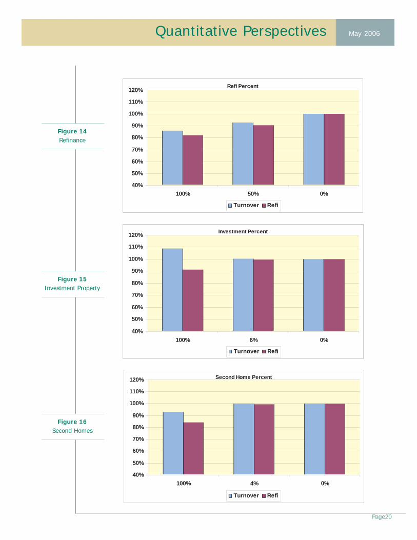
In the few examples we observed, we saw how different classes produced different multipliers for

RefiSMM and TurnoverSMM. Figures 11 though 18 illustrate how the multipliers for the different

variables behave for the turnover and refinance components. Remember there are no multipliers for

the Owner, Purchase, and Single Family categories because they are considered the average

categories. Also, Figures 14 through 18 show what the multiplier effects would be for different

percentages of each data element, since the multiplier is calculated based on the percentage.

Multiplier Overview


Page19

40%50%60%70%80%90%

100%110%120%130%

<50K 50K-75K

75K-100K

100K-125K

125K-150K

150K-175K

175K-200K

200K-225K

225K-250K

>250K

Turnover Refi

Figure 11WAOLB

50%

60%

70%

80%

90%

100%

110%

120%

130%

<55% 55%-65% 65%-70% 70%-75% 75%-80% 80%-90% >90%

Turnover Refi

70%

80%

90%

100%

110%

120%

130%

140%

150%

<670 670-690 690-710 710-730 730-750 >750

Turnover Refi

Figure 13FICO

Figure 12WAOLTV


Page20

Refi Percent

40%

50%

60%

70%

80%

90%

100%

110%

120%

100% 50% 0%

Turnover Refi

Figure 14Refinance

Investment Percent

40%

50%

60%

70%

80%

90%

100%

110%

120%

100% 6% 0%

Turnover Refi

Second Home Percent

40%

50%

60%

70%

80%

90%

100%

110%

120%

100% 4% 0%

Turnover Refi

Figure 15Investment Property

Figure 16Second Homes

What overall trends do we recognize from the previous charts? One main effect is that a lower original

loan balance leads to lower prepayments, and a higher loan balance leads to a higher prepayment for

loans with a refinance incentive. Also, a lower LTV leads to higher turnover, but less refinancing. This

could be due to a variety of reasons, like lower LTV loans having favorable interest rates. Looking at

FICO, it's interesting to note that relative to the 730-750 class, as FICO decreases, turnover increases.

When looking at the datasets, we see that in the Discount dataset that 72% of the balance lies above a

FICO of 730. We also see that as the percentage of both Second Homes and Multifamily properties

increases, the overall prepayment speed decreases. Finally, pools made up of mostly NY loans will have

slower than average prepayment speeds, while those made up of mostly CA loans will be faster.

The APD framework is advantageous for modeling prepayments in this fashion. Since burnout is

endogenous to the model, the rate of burnout naturally adjusts for changes in the relative speeds of the

TurnoverSMM and the RefiSMM. A parametric model of burnout would need to be adjusted to reflect

these changes.


Page21

MultiFamily Percent

40%

50%

60%

70%

80%

90%

100%

110%

120%

100% 4% 0%Turnover Refi

Figure 17Multi Family

0%

20%

40%

60%

80%

100%

120%

140%

NY FL TX CA ILStatesTurnover Refi

Figure 18Geography


Page22

After initially estimating the Pool-Level Prepayment Model, we noticed that the model was

consistently overstating prepayments for loans originated from 1992-1998. Further analysis revealed

that the prepayment model was slightly biased towards more recent data because more loans from

the past 3-4 years are in the dataset compared to loans originated 7-10 years ago. This is not a flaw

in the data, but rather a natural result of prepayments occurring over time. Since the average loan

size has been increasing over time, especially within the last few years, we realized the best way to

slow down prepayments for older vintages was to use the results of our enhanced data multipliers to

scale prepayment forecasts for pools based on their time of origination using a data file of historical

average loan sizes over time. For example, for a pool originated in November 1995, the average size

of a FNMA loan originated at that time was about $105,000. Using this value, we apply the multiplier

corresponding to this WAOLB and scale the RefiSMM and TurnoverSMM accordingly. Since the graphs

from the previous section show that the multipliers decrease as loan size decreases, this is an

effective way to slow down prepayment forecasts for older vintages. This effect is implemented in

the pool level model and is disabled when enhanced data is used, so that the true WAOLB is used

instead of the approximated historical value.

To see the effects of the Enhanced Model in practice, we ran an analysis using the same inputs in

both the Pool Model and the Enhanced Model, but with the addition of WAOLB, WAOLTV, FICO and

geographical breakdown for the Enhanced Model. For this particular example, we analyzed a FNMA

30-year pool with an age of 1 month and a pool WAC of 6.0. We started the analysis in January

2004 and forecast 25 months of prepayment speeds using known mortgage rates. For the enhanced

data we used a WAOLB of $65,000, a WAOLTV of 68%, a FICO of 740, and made the geographical

breakdown to be 100% NY loans. Figure 19 displays the forecasts for both the Pool Model and the

Enhanced Model.

Vintage-Based Loan Size Effect

Enhanced vs. Pool Model

0

5

10

15

20

25

30

35

40

Jan-04

Apr-04

Jul-04Oct-04

Jan-05

Apr-05

Jul-05Oct-05

Jan-06

Date

CPR

Pool Model Enhanced Model

Figure 19


Page23

As we can see, the incorporation of the additional enhanced data factors greatly influences the

prepayment forecast. For this example, we chose inputs determined to have a dampening effect in

order to display the strength of the multipliers of the Enhanced Model. It is possible that given

different characteristics of a pool the various multipliers will almost cancel each other out. Also, if any

characteristics are left blank, they will be set to 100%.

Comparison of v4.3.4 and v5.1 Pool models

On the Pool Model level, there are several major differences between the ADCo Pool Level Prepayment

Model (v4.3.4) and the Enhanced Prepayment Model (v5.1). A quick recap:

1. Burnout: The previous method for modeling burnout has been replaced with the new Active-Passive

Decomposition method. This is a more natural form of capturing the burnout of a given pool, using

that pool's heterogeneity as the driver of burnout.

2. Yield Curve Spread Effect: Using the two and ten year LIBOR rates, we calculate additional or

lessened refinance incentive based on the spread between the two rates. This gives a proxy as to how

favorable it may be to refinance into an ARM depending on whether the yield curve is steep or flat.

3. Vintage-based Loan Size Effect: Given that loan sizes have been increasing over time, we use

this effect to dampen prepayment speeds for older collateral, since a prepayment model estimated in

today's marketplace is biased towards the higher loan balances of the past few years. This factor is

directly derived from the enhanced data multipliers.

We'll now look at comparisons between version 4.3.4 and version 5.1 to get an idea of the differences

between them. In both cases, we are looking at the pool-level models only. First, Figure 20 shows both

models' historical fit for a FNMA 30-year 6.5 originated in 2001. As we can see, version 5.1 pool model

does a better job at reaching peak speeds and has an overall average model error of 2.9 CPR compared

to 5.0 CPR for version 4.3.4.

0

10

20

30

40

50

60

70

80

Jan-01

Apr-01

Jul-01Oct-01

Jan-02

Apr-02

Jul-02Oct-02

Jan-03

Apr-03

Jul-03Oct-03

Jan-04

Apr-04

Jul-04Oct-04

Jan-05

Apr-05

Jul-05Oct-05

CPR

Actual CPR 4.3.4 Model CPR 5.1 Model CPR

Figure 20


Page24

Now we'll take a look at some valuation results in Figure 21 using both 4.3.4 and 5.1 Pool Level

Models. The inputs here (price, WAM and servicing) are market data obtained from Bloomberg on

February 3, 2006. We use the ADCo OAS v5.2 for prepayment model version 4.3.4 and OAS v6.0 for

prepayment model version 5.1, with the same rate and volatility assumptions for both.

Here, it is apparent that durations have shortened across the board and that WALs are less for the

discounts, slightly more around par and less for the premiums. This reflects the change in the way

burnout is modeled, along with the other improvements made to the model.

This release of the Andrew Davidson & Co., Inc. Fixed Rate Agency MBS Pool-Level Prepayment

Model and Enhanced Prepayment Model mark a new modeling approach compared to previous model

versions. The overall structure of the model has been changed, and a new layer of detail has been

added to pool model prepayment forecasting thanks to the new enhanced data elements now

provided by the agencies. The combination of the new model features, the applied APD method of

burnout modeling and the ability to consider enhanced data elements gives this version of the

Andrew Davidson & Co., Inc. Fixed-Rate Agency MBS Prepayment Model a great amount of power in

forecasting prepayments.

v4.3.4

Net

Coupon WAM Serv Price OAS WAL PSA

Effective

Duration

Modified

Duration

Effective

Convexity

FNCL 4.5 354 75 93.64 5 9.23 136 5.27 6.63 -0.6

FNCL 5.0 354 60 96.45 1 8.89 146 4.58 6.35 -1.07

FNCL 5.5 355 45 98.67 2 7.51 194 3.78 5.47 -1.47

FNCL 6.0 349 47 100.73 -3 4.84 319 2.7 3.71 -1.92

FNCL 6.5 337 50 102.33 19 4.8 295 2.48 3.68 -1.48

FNCL 7.0 323 55 103.72 37 4.01 350 2.46 3.25 -0.77

FNCL 7.5 306 62 104.53 48 3.05 455 2.18 2.61 -0.27

FNCL 8.0 298 60 105.94 37 2.63 522 2.04 2.32 0.29

v5.1

Net

Coupon WAM Serv Price OAS WAL PSA

Effective

Duration

Modified

Duration

Effective

Convexity

FNCL 4.5 354 75 93.64 1 8.56 154 5.19 6.09 -0.58

FNCL 5.0 355 60 96.42 -5 7.64 188 4.51 5.52 -1.07

FNCL 5.5 356 45 98.64 -5 6.82 225 3.74 5.02 -1.51

FNCL 6.0 349 47 100.73 -13 5.26 290 2.49 4.04 -2.04

FNCL 6.5 339 50 102.3 -8 3.71 390 1.93 3.02 -1.7

FNCL 7.0 323 55 103.72 4 3.25 430 1.82 2.75 -1.08

FNCL 7.5 306 62 104.53 9 2.56 534 1.51 2.26 -0.45

FNCL 8.0 297 60 105.94 -3 2.3 586 1.42 2.08 0.13

Figure 21

Conclusion


Page25

[1] "Home Price & Prepayments: The New Andrew Davidson & Co., Inc. Prepayment Model,"

Quantitative Perspectives, Andrew Davidson & Co., Inc., July 2001.

[2] "The Relationship between the Yield Curve and Mortgage Current Coupon," Quantitative

Perspectives, Andrew Davidson & Co., Inc. April 2001.

[3] "Divide and Conquer: Exploring New OAS Horizons, Parts I, II, & III," Quantitative Perspectives,

Andrew Davidson & Co., Inc., June 2004.

Dan Szakallas is responsible for the research and development of the company's suite of Agency pool-

level prepayment models for both fixed rate and ARM collateral using data from Fannie Mae, Freddie

Mac, and Ginnie Mae. He has worked extensively in incorporating the Active-Passive Decomposition

mortgage model as well many other factors into the proprietary models developed at Andrew

Davidson & Co., Inc. He also provides custom model tuning analysis to clients using their portfolio

data and monitors model performance using the dynamic performance reports available at the Andrew

Davidson & Co., Inc. website www.ad-co.com.

In addition, Dan has co-authored several of Andrew Davidson & Co., Inc.'s Quantitative Perspectives,

has had an article published in the Journal of Fixed Income, and regularly contributes his model

performance analysis to the company's monthly newsletter, The Pipeline.

He graduated from Carnegie Mellon University with a dual major in Statistics and Psychology.

Works Referenced

Author Biography

ANDREW DAVIDSON & CO., INC.520 BROADWAY, EIGHTH FLOORNEW YORK, NY 10012212-274-9075FAX [email protected]

QUANTITATIVE PERSPECTIVES is available via www.ad-co.com

We welcome your comments and suggestions.

Contents set forth from sources deemed reliable, but Andrew Davidson & Co., Inc. does not guarantee its

accuracy. Our conclusions are general in nature and are not intended for use as specific trade recommendations.

Copyright 2006

Andrew Davidson & Co., Inc.

QP


qp - ad&co · pdf fileqp. introduction the andrew davidson ... the model incorporates the...

Documents