QE in the future: managing the size and

composition of the central bank’s balance

sheet in a fiscal crisis∗

Ricardo Reis

Columbia University and LSE

31st of July, 2015

Abstract

Arguments for quantitative easing (QE) typically rely on the economy being in

either a financial crisis, or with nominal interest rates at zero, or both. This paper

examines the usefulness of QE in a fiscal crisis, modeled as a situation where the fiscal

outlook is inconsistent with both stable inflation and no default on government bonds.

The crisis can lower welfare through three channels: via nominal rigidities, via losses

in the banking sector’s net worth, and via a glut of safe assets that financial markets

need to function. Managing the size and composition of the central bank’s balance

sheet can interfere with each of these channels, and so stabilize inflation and economic

activity, minimizing the welfare losses during a fiscal crisis.

∗Contact: rreis@columbia.edu. An earlier draft of this paper was given as the keynote address at theBanco Central do Brasil XVII Inflation Targeting seminar.

1 Introduction

At the start of the 2008 financial crisis, central banks engaged in unconventional policies,

buying many risky assets and giving credit to a wide variety of private agents.1 Just a few

years later, the balance sheets of the the Bank of England, the Bank of Japan, the ECB, and

the Federal Reserve became dominated by only a few items. On the liabilities size, almost

entirely a large stock of reserves paying interest. On the asset side, there is a portfolio of

securities either issued directly by the government or backed by it, together with foreign

currency. These major four central banks actively used quantitative easing (QE) policies

consisting of deciding on the size of the balance sheet of the central bank—the amount of

reserves—and its composition—the maturity of the bonds held.2

The motivation for these policies was the combination of a financial crisis and zero nom-

inal interest rates, and the desire to stimulate inflation and real activity. The stated goals

of QE were to increase liquidity, to commit to keeping interest rates at zero for prolonged

period of time, and to lower long-term yields (Bernanke, 2015). The economic theory to

justify issuing reserves to buy short-term and long-term government bonds relied on models

where short-term interest rates are zero (Bernanke and Reinhart, 2004) or on models where

frictions in credit markets prevent arbitrage across asset classes and drive changes in term

premia (Vayanos and Vila, 2009; Gertler and Karadi, 2013).

The financial crisis is now several years behind. Interest rates in the United States

are expected to take off from zero in 2016, and will eventually do so in the other central

banks. When this happens, will QE disappear, as did so many of the other unconventional

monetary policies? Is there a use for QE policies in a future where there is no financial crisis

and nominal interest rates are positive? Under what circumstances, if any, can QE have any

effect on the targets of the central bank?

This paper writes down a simple model of fiscal and monetary policy where, in normal

times, QE is neutral. However, during a fiscal crisis, the central bank’s management of its

balance sheet can have a powerful effect on outcomes. The focus on fiscal crisis is motivated

by the current data: public debt in the United Kingdom, Japan, many European countries,

and the United States is at historically high levels. It is plausible, perhaps even likely, that

the next macroeconomic crisis will be fiscal, as suggested by the recent experience in Greece.

1Reis (2009) surveys these unconventional monetary policies.2The literature describing these policies and measuring their impact includes event studies on the re-

sponses of yields (e.g., Krishnamurthy and Vissing-Jorgensen, 2011), estimated DSGEs on macroeconomicvariables (e.g., Chen, Curdia, and Ferrero, 2012), and instrumental-variables regressions on loan supply (e.g.,Morais, Peydro, and Ruiz, 2015).

1

Moreover, while the literature has focussed on understanding QE during a financial crisis,

there is no comparable work on the role of QE when the source of the problems is fiscal.

I identify three channels through which QE can matter for equilibrium outcomes in a

fiscal crisis. First, the composition of the central bank’s balance sheet alters the composition

of the privately-held public debt. In turn, this affects the sensitivity of inflation to fiscal

shocks. It is well understood that, after a fiscal shock that makes anticipated fiscal surpluses

fall short of paying for the outstanding debt then, without default, the price level must

increase to lower the real value of the debt. Less appreciated is that the maturity of the

combined government debt and bank reserves held by the public determines the size of this

bout of inflation. I show that while QE cannot affect expected inflation, it can influence how

volatile is the response of the price level to fiscal shocks. Because it is unexpected inflation

that matters for welfare, by inducing firms with old information to make mistakes when

choosing their prices, QE can reduce the welfare costs associated with surprise inflation.

The second channel comes through the costs of default. Banks hold government bonds so,

following a default, they suffer losses that lower their equity. Because bank equity constrains

lending, following a government default, there is a credit crunch that lowers real activity

and welfare. Anticipating a default, the central bank can issue reserves and buy government

bonds from the banks, taking this risk from their balance sheet. In doing so, the central

bank takes onto its balance sheet the losses from government default, preserving the banking

system. In the model in this paper this raises welfare. However, since the central bank losses

are eventually passed to the fiscal authority through smaller dividends from the central bank,

QE is effectively redistributing resources to the banks from the other holders of government

bonds in the economy.

The third channel is through the provision of safe assets. If default seems likely, financial

markets may freeze due to the absence of safe collateral. By expanding the stock of reserves

and purchasing long-term government bonds, the central bank can supply this demand for

safety and lower real interest rates, promoting investment by relaxing financial constraints.

The goal of this paper is to highlight these three channels. Each of them comes with

caveats and limitations, some captured by the model, and others that I discuss. QE may be

met with changes in maturity management by the Treasury, it may affect the incentives for

sovereigns to default, and it may lead to central bank insolvency. The interaction with fiscal

authorities always jointly determines macroeconomic outcomes, and QE policies make this

interdependence more visible. By isolating the assumptions needed for the three channels to

be operative, this paper aims to open the possibility of discussing whether and when QE is

2

effective and desirable.

Section 2 presents the model and its assumptions. Section 3 discusses two starting bench-

marks. First, it studies the case where there is no fiscal crisis, in which case QE is neutral.

Second, it reexamines Wallace neutrality, showing that, in the model, open market operations

where reserves are exchanged for short-term government bonds are neutral.

Section 4 focuses on inflation. Using the fiscal theory of the price level, it builds on

Cochrane (2001, 2014) to show that QE affects the sensitivity of inflation to a fiscal shock.3

Expected inflation is pinned down by the nominal interest rate, but QE determines how much

of the fiscal crisis transmits into higher unexpected inflation. I discuss the assumptions on

which this result lies and their plausibility.

Section 5 turns the focus to sovereign default. Building on Uribe (2006), there is only

domestic default since the economy is closed. Of lateral importance, this paper provides

a joint framework to understand sovereign default and the fiscal theory of the price level.

Following Balloch (2015) and Perez (2015), domestic banks use reserves as well as short-term

public debt in order to borrow in interbank markets. Because banks hold domestic bonds,

sovereign default lowers bank equity, contracts credit, and lowers output. QE changes the

exposure of banks to government bonds, and so affects the losses that result from sovereign

default.

Section 6 focuses on the supply and demand for safe assets, and on the role of QE

for affecting these. Both the size as well as the composition of the central bank’s balance

sheet affect the relative supply for safe assets. By engaging in QE, the central bank affects

investment and output through a safety channel.

Section 7 discusses some of the limitations of QE, and how the assumptions made in the

model rule out some potential pitfalls. Finally, section 8 concludes.

2 A model of monetary policy in a fiscal crisis

Time is indexed by t and goes from date 0 to infinity. Aside from the fiscal authority and the

central bank, there is a private sector, which is composed of consumers, bankers and firms.

I present each of these agents in turn.

3A related paper is Corhay, Kung, and Morales (2014), but they focus on modeling movements in bondpremia, and on the effects of policy at the zero lower bound.

3

2.1 The fiscal authorities

Governments issue liabilities of many different kinds. Central banks, however, tend to focus

their operations on the more liquid bonds issued by fiscal authorities. In part, this is so that

the value of the assets bought by the central bank can be inferred from market prices, and so

the operation of monetary policy does not involve transfers to the fiscal authorities by over-

paying to the Treasury for the assets it issues. The emphasis on central bank independence

and on transparency requires that transfers between these two arms of the government is

transparent.

Of the liquid assets issued by the Treasury, the more dominant are nominal bonds of

different maturities. While the maturity structure of the outstanding public debt can be

complex, in the model I simplify by considering only two types: 1-period and 2-period

bonds. While the points that I will make would extend to more varied maturities, focusing

on these, short and long-term, bonds simplifies the analysis. The goal of the model is to

highlight economic channels qualitatively, rather than quantify their effect.

The amount of bonds outstanding at date t that mature in one period is denoted by bt

and they trade for price qt. These include both long-term bonds issued at t − 1 as well as

short-term bonds just issued: they are equivalent from the perspective of date t. Long-term

bonds issued at date t trade at price Qt and pay Bt at t+2. The prices are in nominal units,

and the price level is pt.

The government receives a real dividend from the central bank dt and chooses a real

fiscal surplus ft. Higher surpluses are costly because of the distortionary effects of taxation

or because of the valuable social services that are lost by cutting on government spending.

I model these costs in a stark way: the fiscal authority can costlessly choose any ft < ft,

but it is infinitely costly to generate higher fiscal surpluses. A perspective on the fiscal limit

ft is that it is the peak of the Laffer curve, the upper bound on what the government can

collect from its citizens without leading to widespread tax evasion. A fiscal crisis is then a

contraction in ft.

The government flow budget is:

δt(bt−1 + qtBt−1) = pt(ft + dt) + qtbt +QtBt. (1)

The variable δt ∈ [0, 1] is the repayment rate at date t on bonds that were outstanding. When

δt = 1, debts are honored. Otherwise, 1− δt is the haircut suffered by the bondholders.

4

In turn, the intertemporal budget constraint of the government is:(δtpt

)(bt−1 + qtBt−1) = Et

[∞∑τ=0

mt,t+τ (ft+τ + dt+τ )

]. (2)

Future uncertain payoffs are priced by a stochastic discount factor mt,t+τ . Another way to

write this constraint would be to state that the government debt cannot be a Ponzi scheme.4

Fiscal policy consists of picking surpluses {ft} and debt management {δt, bt, Bt}, which

includes both whether and how much to repay old debts, as well as how to manage the

maturity of outstanding debt.

2.2 The central bank and QE

The central bank buys the two government bonds. Its holdings are denoted by bct and Bct . On

its liabilities, the central bank issues reserves vt, which are held exclusively by banks. Since

the central bank can always repay banks by issuing more reserves, there is never default in

the amount of outstanding reserves. The central bank chooses the interest rate it to pay to

the holders of reserves.

Aside from financing the purchase of assets, the issuance of liabilities finances the gap

between the dividend that the central bank pays the fiscal authority, dt, and the seignorage

revenue it earns from issuing currency st. Central banks earn seignorage insofar as private

agents chose to hold currency even though it does not pay a market interest rate. While

higher inflation affects seignorage, both by debasing its real value and by affecting the desire

to hold currency, Hilscher, Raviv, and Reis (2014b) find empirically that the elasticity of

seignorage with respect to inflation is quite small. For simplicity, I therefore take seignorage

net of expenses st to be exogenous.

Combining all these ingredients, the flow budget of the central bank is:

vt − vt−1 = it−1vt−1 + qtbct +QtB

ct − δt(bct−1 + qtB

ct−1) + pt(dt − st) (3)

The central bank cannot run a Ponzi scheme on reserves, otherwise their real value would

be zero. Because reserves are the unit of account in the economy, their real value is 1/pt, so

if there was a Ponzi scheme, the price level would be infinity. The intertemporal constraint

4The associated no Ponzi scheme constraint is: limT→∞ Et[δt+T (bt+T−1 + qt+TBt+T−1)/pt+T ] = 0.

5

on the central bank then is:

(1 + it−1)vt−1 − δt(bct−1 + qtBct−1)

pt= Et

[∞∑τ=0

mt,t+τ (st+τ − dt+τ )

](4)

A fiscal authority in a crisis will most likely not be willing to bail out its central bank. The

historical experience rather suggests the opposite: during a fiscal crisis, the Treasury tries

to extract more resources from the central bank forcing it to raise inflation in order to earn

more seignorage to rebate to the Treasury (Sargent, 1982). I assume that the central bank

manages to keep its independence, so st is independent of the crisis, but the central bank

does not have unlimited fiscal backing from the Treasury, so it must avoid insolvency. There

are different possible types of insolvency for a central bank depending on the relationship

between the central bank and the fiscal authority (Reis, 2015), and here I assume the weakest

of these, intertemporal solvency: Et (∑∞

τ=0 mt,t+τdt+τ ) ≥ 0.

Given these constraints, monetary policy consists of choices of the interest rate paid on

reserves {it} and balance-sheet policies {vt, bct , Bct}. Some of these may follow rules, they do

not need to be exogenous.

The central bank could choose to issue zero reserves and hold zero bonds, while still

setting interest rates and rebating seignorage in full every period. This is the typical case

considered in studies of monetary policy (Woodford, 2003). Quantitative easing, the focus of

this paper, consists of changes in the balance sheet such that: vt = qtbct+QrB

ct , so the central

bank issues reserves to buy short-term and/or long-term government bonds. Quantitative

easing policies consists of the twin choices by the central bank of how many reserves to issues,

and what maturity of government bonds to acquire with them.

2.3 Households

A representative household has preferences given by:

Et

[∞∑τ=0

βτu

(ct+τ −

l1+αt+τ

1 + α

)], (5)

where u(.) : R → R with u′(.) ≥ 0 and u′′(.) ≤ 0 is the household’s utility function, ct is

aggregate consumption and lt are hours worked. The particular functional form inside the

utility function implies that there are no income effects on hours worked, and that α is the

6

inverse of the wage-elasticity of labor supply, since the optimal labor supply is:

lαt = wt/pt (6)

where wt is the wage rate.

Households can choose to hold any of the financial assets across periods, either directly, or

in the case of reserves, indirectly via banks. Therefore, the following no-arbitrage conditions

must hold:

Et(mt,t+1δt+1ptqtpt+1

)= Et

(mt,t+2δt+1δt+2pt

Qtpt+2

)= Et

(mt,t+1(1 + it)pt

pt+1

)= 1. (7)

The stochastic discount factor is, as usual, equal to the discounted marginal utility in the

future as a ratio of marginal utility today. Note that, while the central bank can choose the

interest paid on reserves, for banks to want to voluntarily hold them and so for the price

level to be finite, reserves must pay a market interest rate.

2.4 Firms

Aggregate output yt is a Dixit-Stiglitz aggregator of a continuum of varieties of goods:

yt =

(kθt

∫ kt

0

yt(j)σ−1σ dj

) σσ−1

, (8)

where σ > 1 is the elasticity of demand for each individual variety. The measure of varieties

available for production is denoted by kt and can vary over time, with the strength of the

“love for variety” determined by the parameter θ.

The reason for using kt to denote varieties is that each variety can be produced by a

single monopolistic firm as long as it has one unit of capital to use. Therefore the number of

varieties is the same as the amount of capital employed in the economy, or the measure of

firms in operation. Capital is available from banks for rental at price 1 + rt. Because there

is free entry, firms expect to earn zero profits in this monopolistic competition equilibrium.

Once they have installed their capital, firms operate a production function yt(j) = Atlt(j)

by hiring labor lt(j) with productivity At. Market clearing in the labor market is then given

by lt =∫lt(j)dj. Standard calculations show that the desired optimal price is a constant

7

markup over marginal cost:

p∗t =

(σ

σ − 1

)wt. (9)

However, only a fraction λ of firms can choose their price equal to their desired level.

The remainder must choose their prices with one-period old information, and set them

approximately equal to Et−1(p∗t ). Because all firms are ex ante identical, this price dispersion,

∆t, is an inefficiency that leads to under-production. Aggregating across firms:

∆t

∫yt(j)dj = Alt, (10)

∆t ≡(p∗tpt

)−σ [λ+ (1− λ)

(Et−1(p∗t )

p∗t

)−σ]≥ 1 (11)

2.5 Banks, the interbank market, and credit

Every period, the economy receives an endowment of capital of one unit that fully depreciates

by the end of the period. Capital can be turned one-to-one into consumption, or used to

produce varieties of goods. However, capital must make its way to the firms through a

financial system with frictions, modeled in a way inspired by Gertler and Kiyotaki (2010),

Bolton and Jeanne (2011), and Balloch (2015). A fraction κ of the capital is owned by banks,

while the remaining 1− κ belongs to households. In turn, only a fraction ω of the banks is

matched with firms and productive possibilities, while the remaining 1− ω only have access

to an interbank market in which they can trade with other banks.

Banks without opportunities can return their capital to households as dividends for con-

sumption, earning a return of 1. Alternatively, at the start of the period, before uncertainty

has been realized and goods and labor markets open, the interbank market opens where

they can lend xt to productive banks. The feasibility constraint on interbank lending is:

xt ≤ (1− ω)κ.

Banks with opportunities can either lend them to firms or hold short-term government

bonds and reserves. Government bonds will be worth δt ≤ 1 by the end of the period, so

the bank would prefer to lend its capital out. However, with the amount xt they receive in

interbank loans, banks can only commit to repay back a share ξ ≤ 1. They must deposit a

share 1 − ξ in bonds on reserves to receive the interbank loans. This leads to the incentive

8

constraint:

xt ≤Et−1(δt)b

pt−1 + vt−1

1− ξ(12)

where bpt−1 are the bond holdings by borrowing banks at the start of the period, before date

t information is revealed. With a large ξ, the relevant case, banks hold a few bonds that

allow them to borrow large amounts in interbank markets.

The interbank market is senior to the other market where banks with opportunities obtain

funding: the deposit market. This market, where banks deal with households, opens during

the period, after uncertainty has been realized. Deposits, ht, face a feasibility constraint

ht ≤ 1− κ. If the bank pays a return on deposits above 1, the rate at which households can

transform capital into consumption, then this constraint binds. Otherwise, and this will be

the relevant case, the return on deposits will be 1.

This is because, aside from feasibility, there is also an incentive constraint. Banks can

only pledge a share γ of their revenues, but can abscond with the remainder. For them to

choose not to do so, it must be that their return from paying depositors in full exceeds that

from absconding, so:

(1 + rt)(nt + ht)− ht ≥ (1− γ)(1 + rt)(nt + ht), (13)

where nt is the bank’s net worth. Since the bank started with capital ωκt, fully collateralizes

and pays loans in the interbank market, but holds bonds that may have defaulted, the net

worth is: nt = ωκt − bpt−1(1− δt).The combined effect of these two frictions, in interbank and deposit markets, is that the

unit of capital available in the economy will end up funding only kt projects, the sum of the

capital in productive banks, the capital raised in interbank markets minus what is tied up

in the interbank market, plus the amount raised as deposits net of losses in the collateral

portfolio:

kt = ωκ+ xt − (Et−1(δt)bpt + vt) + ht − bpt−1(1− δt) ≤ 1. (14)

At the end of the period, banks return their profit to the households. Total consumption is

the sum of what was produced by firms, and what was not used as capital: ct = yt + 1− kt.

9

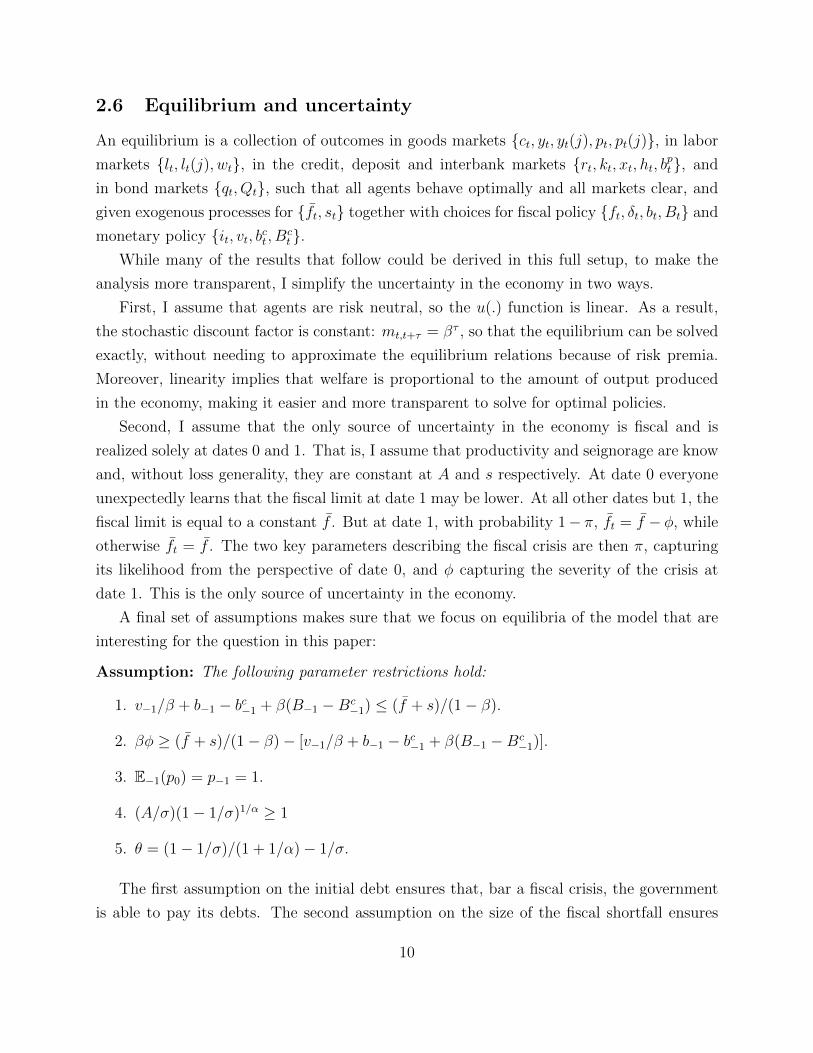
2.6 Equilibrium and uncertainty

An equilibrium is a collection of outcomes in goods markets {ct, yt, yt(j), pt, pt(j)}, in labor

markets {lt, lt(j), wt}, in the credit, deposit and interbank markets {rt, kt, xt, ht, bpt}, and

in bond markets {qt, Qt}, such that all agents behave optimally and all markets clear, and

given exogenous processes for {ft, st} together with choices for fiscal policy {ft, δt, bt, Bt} and

monetary policy {it, vt, bct , Bct}.

While many of the results that follow could be derived in this full setup, to make the

analysis more transparent, I simplify the uncertainty in the economy in two ways.

First, I assume that agents are risk neutral, so the u(.) function is linear. As a result,

the stochastic discount factor is constant: mt,t+τ = βτ , so that the equilibrium can be solved

exactly, without needing to approximate the equilibrium relations because of risk premia.

Moreover, linearity implies that welfare is proportional to the amount of output produced

in the economy, making it easier and more transparent to solve for optimal policies.

Second, I assume that the only source of uncertainty in the economy is fiscal and is

realized solely at dates 0 and 1. That is, I assume that productivity and seignorage are know

and, without loss generality, they are constant at A and s respectively. At date 0 everyone

unexpectedly learns that the fiscal limit at date 1 may be lower. At all other dates but 1, the

fiscal limit is equal to a constant f . But at date 1, with probability 1− π, ft = f − φ, while

otherwise ft = f . The two key parameters describing the fiscal crisis are then π, capturing

its likelihood from the perspective of date 0, and φ capturing the severity of the crisis at

date 1. This is the only source of uncertainty in the economy.

A final set of assumptions makes sure that we focus on equilibria of the model that are

interesting for the question in this paper:

Assumption: The following parameter restrictions hold:

1. v−1/β + b−1 − bc−1 + β(B−1 −Bc−1) ≤ (f + s)/(1− β).

2. βφ ≥ (f + s)/(1− β)− [v−1/β + b−1 − bc−1 + β(B−1 −Bc−1)].

3. E−1(p0) = p−1 = 1.

4. (A/σ)(1− 1/σ)1/α ≥ 1

5. θ = (1− 1/σ)/(1 + 1/α)− 1/σ.

The first assumption on the initial debt ensures that, bar a fiscal crisis, the government

is able to pay its debts. The second assumption on the size of the fiscal shortfall ensures

10

that there is a fiscal crisis. The third assumption pins down the initial conditions for prices

and expectations at the convenient value of 1. The fourth assumption guarantees that

productivity is high enough so that it is socially optimal to use capital for production rather

than consumption.

The fifth assumption is more peculiar and deserves some explanation. It fixes the love for

variety as a precise formula of the elasticities of product demand and labor supply. It is well

known that in monopolistic competition models like this one, the profits of an individual

firm may increase or decrease as more firms enter the market. On the one hand, as more

firms enter, the demand for each variety declines, keeping total spending fixed. On the other

hand, total output increases because of an externality, since more varieties produced raise

overall welfare and demand for all goods. The parameter θ controls the strength of this

second effect relative to the first. Making this particular assumption on its value results in

the return on each firm earned by the bank, rt being constant. This simplifies the analysis

considerably, while losing little in terms of the generality of the results.

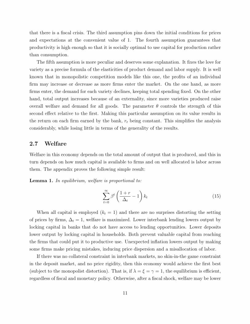
2.7 Welfare

Welfare in this economy depends on the total amount of output that is produced, and this in

turn depends on how much capital is available to firms and on well allocated is labor across

them. The appendix proves the following simple result:

Lemma 1. In equilibrium, welfare is proportional to:

∞∑t=0

βt(

1 + r

∆t

− 1

)kt (15)

When all capital is employed (kt = 1) and there are no surprises distorting the setting

of prices by firms, ∆t = 1, welfare is maximized. Lower interbank lending lowers output by

locking capital in banks that do not have access to lending opportunities. Lower deposits

lower output by locking capital in households. Both prevent valuable capital from reaching

the firms that could put it to productive use. Unexpected inflation lowers output by making

some firms make pricing mistakes, inducing price dispersion and a misallocation of labor.

If there was no collateral constraint in interbank markets, no skin-in-the game constraint

in the deposit market, and no price rigidity, then this economy would achieve the first best

(subject to the monopolist distortion). That is, if λ = ξ = γ = 1, the equilibrium is efficient,

regardless of fiscal and monetary policy. Otherwise, after a fiscal shock, welfare may be lower

11

because of the three frictions in the economy: nominal rigidities by firms leading to price

dispersion, credit frictions in collecting funds from depositors, and liquidity frictions in the

interbank market. It is through each of these frictions that each of the three channels in this

paper operate.

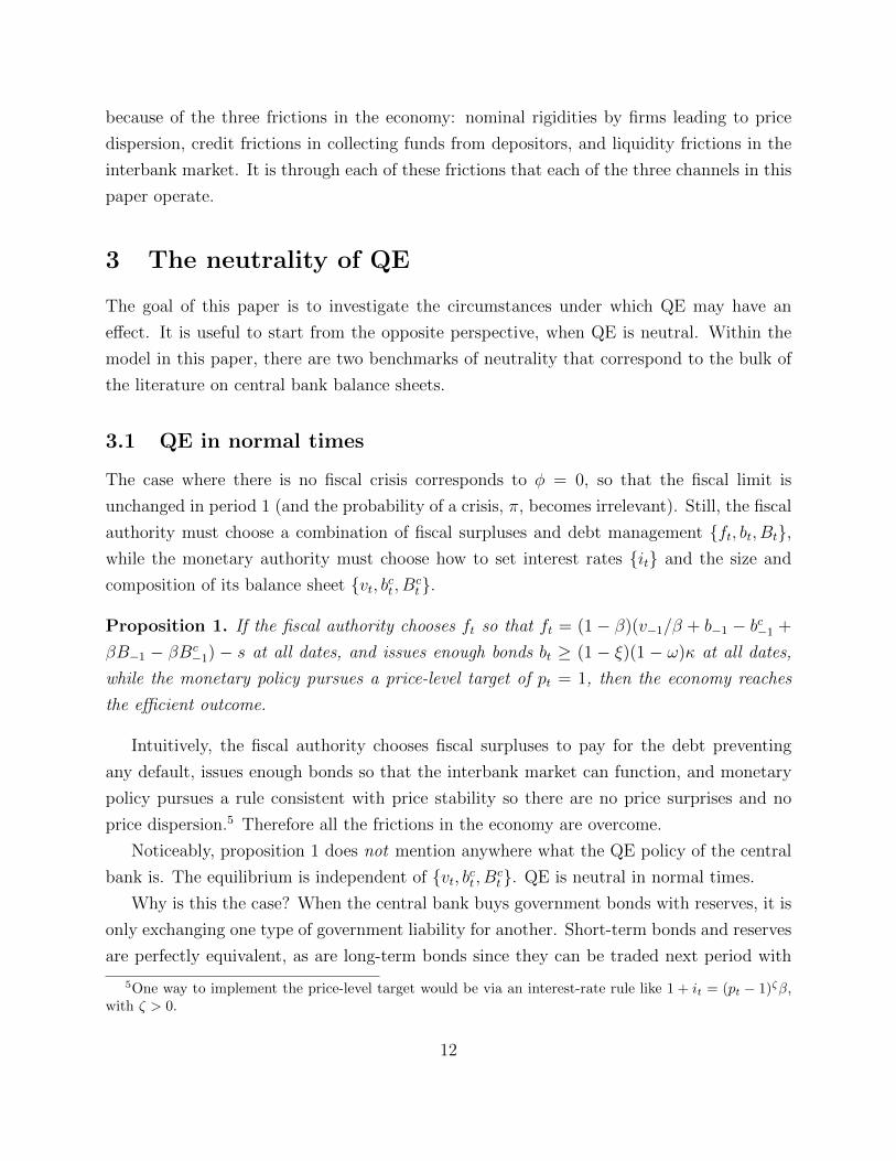
3 The neutrality of QE

The goal of this paper is to investigate the circumstances under which QE may have an

effect. It is useful to start from the opposite perspective, when QE is neutral. Within the

model in this paper, there are two benchmarks of neutrality that correspond to the bulk of

the literature on central bank balance sheets.

3.1 QE in normal times

The case where there is no fiscal crisis corresponds to φ = 0, so that the fiscal limit is

unchanged in period 1 (and the probability of a crisis, π, becomes irrelevant). Still, the fiscal

authority must choose a combination of fiscal surpluses and debt management {ft, bt, Bt},while the monetary authority must choose how to set interest rates {it} and the size and

composition of its balance sheet {vt, bct , Bct}.

Proposition 1. If the fiscal authority chooses ft so that ft = (1 − β)(v−1/β + b−1 − bc−1 +

βB−1 − βBc−1) − s at all dates, and issues enough bonds bt ≥ (1 − ξ)(1 − ω)κ at all dates,

while the monetary policy pursues a price-level target of pt = 1, then the economy reaches

the efficient outcome.

Intuitively, the fiscal authority chooses fiscal surpluses to pay for the debt preventing

any default, issues enough bonds so that the interbank market can function, and monetary

policy pursues a rule consistent with price stability so there are no price surprises and no

price dispersion.5 Therefore all the frictions in the economy are overcome.

Noticeably, proposition 1 does not mention anywhere what the QE policy of the central

bank is. The equilibrium is independent of {vt, bct , Bct}. QE is neutral in normal times.

Why is this the case? When the central bank buys government bonds with reserves, it is

only exchanging one type of government liability for another. Short-term bonds and reserves

are perfectly equivalent, as are long-term bonds since they can be traded next period with

5One way to implement the price-level target would be via an interest-rate rule like 1 + it = (pt − 1)ζβ,with ζ > 0.

12

no risk. Therefore, QE has no effect on the solvency of the government, on its ability to pay

for is debts, and therefore on the price level or on the likelihood of default.

Mathematically, this can be seen because the consolidated government budget constraint

only includes reserves in a term: (1 + it−1)vt−1 + bt−1 − bct−1 + qt(Bt − Bct ). Any QE policy

consist of exchanging reserves for government bonds. But, the arbitrage condition linking

it, qt and Qt ensures that such a purchase would leave this expression unchanged.

In turn, in credit markets, reserves can be equally used as government bonds in the

interbank market. If banks have enough short-run bonds to satisfy their needs in interbank

markets, then no supply of reserves in exchange for these bonds has an effect on the credit

constraints. Again, the two types of government liabilities are perfect substitutes, so that

QE has no effect on the amount of credit in the economy or on the efficiency with which

capital is allocated.

3.2 Wallace neutrality

Another useful benchmark applies even to circumstances when there is a fiscal crisis. As

emphasized by Wallace (1981) and Eggertsson and Woodford (2003), short-term bonds and

reserves are just two forms of government liabilities. Each is denominated in nominal terms,

and promises a certain nominal return next period. Therefore, one would expect that open

market operations, which trade reserves for short-term bonds, have no effect on equilibrium

outcomes. In turn, trading reserves for long-term government bonds is likewise neutral since

with frictionless markets, arbitrage across maturities ensures that the relative quantities

outstanding also do not matter. QE policies and the central bank balance sheets do not

matter.

This is no longer the case if the fiscal crisis can lead to default. Short-term government

bonds and reserves are not perfect substitutes once one allows for default, and neither are

long-term bonds. Central banks never default on reserves. Reserves can only be redeemed for

currency, but the central bank can both print currency and expand or retire reserves at will,

so there is never a need to default on reserves. Short-term government bonds, on the other

hand, can and are defaulted on. Therefore, when default is possible, open market operations

will, in general, affect equilibrium, including the choice by the authority to default or not.

If there is no default, so δt = 1 at all dates, then it is easy to check that in all the

equilibrium conditions in the model only the sum vt + qtbt appears even in the period of

a fiscal crisis. Therefore, exchanging reserves for short-terms bonds is neutral. Yet, as the

next section will show, exchanging reserves for long-term government bonds does have an

13

effect, even when there is no default.

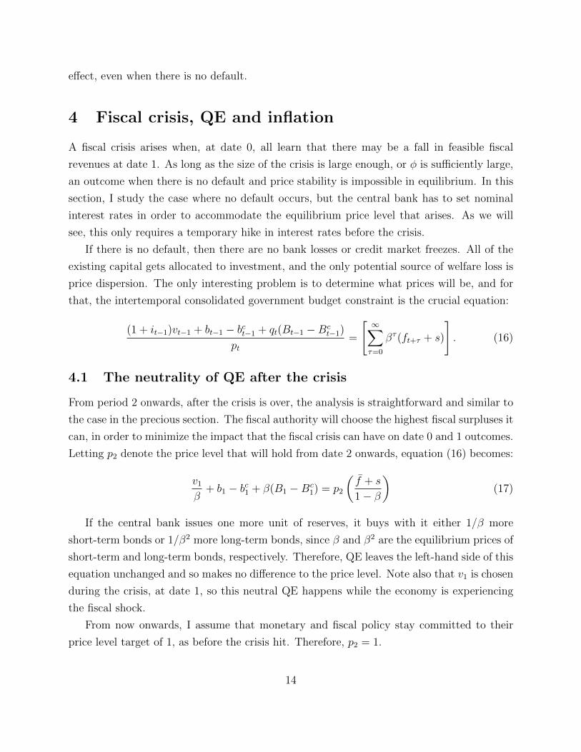
4 Fiscal crisis, QE and inflation

A fiscal crisis arises when, at date 0, all learn that there may be a fall in feasible fiscal

revenues at date 1. As long as the size of the crisis is large enough, or φ is sufficiently large,

an outcome when there is no default and price stability is impossible in equilibrium. In this

section, I study the case where no default occurs, but the central bank has to set nominal

interest rates in order to accommodate the equilibrium price level that arises. As we will

see, this only requires a temporary hike in interest rates before the crisis.

If there is no default, then there are no bank losses or credit market freezes. All of the

existing capital gets allocated to investment, and the only potential source of welfare loss is

price dispersion. The only interesting problem is to determine what prices will be, and for

that, the intertemporal consolidated government budget constraint is the crucial equation:

(1 + it−1)vt−1 + bt−1 − bct−1 + qt(Bt−1 −Bct−1)

pt=

[∞∑τ=0

βτ (ft+τ + s)

]. (16)

4.1 The neutrality of QE after the crisis

From period 2 onwards, after the crisis is over, the analysis is straightforward and similar to

the case in the precious section. The fiscal authority will choose the highest fiscal surpluses it

can, in order to minimize the impact that the fiscal crisis can have on date 0 and 1 outcomes.

Letting p2 denote the price level that will hold from date 2 onwards, equation (16) becomes:

v1

β+ b1 − bc1 + β(B1 −Bc

1) = p2

(f + s

1− β

)(17)

If the central bank issues one more unit of reserves, it buys with it either 1/β more

short-term bonds or 1/β2 more long-term bonds, since β and β2 are the equilibrium prices of

short-term and long-term bonds, respectively. Therefore, QE leaves the left-hand side of this

equation unchanged and so makes no difference to the price level. Note also that v1 is chosen

during the crisis, at date 1, so this neutral QE happens while the economy is experiencing

the fiscal shock.

From now onwards, I assume that monetary and fiscal policy stay committed to their

price level target of 1, as before the crisis hit. Therefore, p2 = 1.

14

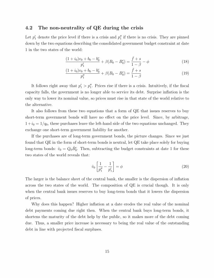
4.2 The non-neutrality of QE during the crisis

Let p′1 denote the price level if there is a crisis and p′′1 if there is no crisis. They are pinned

down by the two equations describing the consolidated government budget constraint at date

1 in the two states of the world:

(1 + i0)v0 + b0 − bc0p′1

+ β(B0 −Bc0) =

f + s

1− β− φ (18)

(1 + i0)v0 + b0 − bc0p′′1

+ β(B0 −Bc0) =

f + s

1− β(19)

It follows right away that p′1 > p′′1. Prices rise if there is a crisis. Intuitively, if the fiscal

capacity falls, the government is no longer able to service its debt. Surprise inflation is the

only way to lower its nominal value, so prices must rise in that state of the world relative to

the alternative.

It also follows from these two equations that a form of QE that issues reserves to buy

short-term government bonds will have no effect on the price level. Since, by arbitrage,

1+ i0 = 1/q0, these purchases leave the left-hand side of the two equations unchanged. They

exchange one short-term government liability for another.

If the purchases are of long-term government bonds, the picture changes. Since we just

found that QE in the form of short-term bonds is neutral, let QE take place solely for buying

long-term bonds: v0 = Q0Bc0. Then, subtracting the budget constraints at date 1 for these

two states of the world reveals that:

v0

[1

p′′1− 1

p′1

]= φ (20)

The larger is the balance sheet of the central bank, the smaller is the dispersion of inflation

across the two states of the world. The composition of QE is crucial though. It is only

when the central bank issues reserves to buy long-term bonds that it lowers the dispersion

of prices.

Why does this happen? Higher inflation at a date erodes the real value of the nominal

debt payments coming due right then. When the central bank buys long-term bonds, it

shortens the maturity of the debt help by the public, so it makes more of the debt coming

due. Thus, a smaller price increase is necessary to being the real value of the outstanding

debt in line with projected fiscal surpluses.

15

4.3 Outlook at the outset of the crisis

If instead of subtracting the budget constraints at the two states in period 1, you multiply

them by their probabilities and add them, one gets the result that

(v0 + b0 − b0c)E0

(1

p1

)+ β(B0 −Bc

0) =f + s

1− β− φ(1− π). (21)

The deeper and more likely the crisis, the larger has to be the increase in expected prices.

However, the increase in E0(1/p1) is independent of QE. Because the inverse function is

convex, then larger QE that lowers the dispersion of prices will lower expected inflation as

well (but not affect its inverse).

Turning then to the date 0 version of equation (16), it is:

v−1/β + b−1 − bc−1

p0

+ β(B−1 −Bc−1)E0

(1

p1

)=f + s

1− β− βφ(1− π) (22)

The prospect of a crisis next period raises prices at date 0, relative to when no crisis is

foreseen (π = 1). Yet, since E0(1/p1) is independent of QE, so is p0. The central bank’s

policies at date 0 will not affect the price level then. All they do is affect the price level next

period, but only in its sensitivity to the fiscal shock occurring.

4.4 Fiscal policy and the limits of QE

Curiously, an observer of this policy may interpret QE as monetary financing of the gov-

ernment during a fiscal crisis. But this is not the case as long as the purchase of long-term

bonds is financed with interest-paying reserves instead of currency. The latter comes with

higher seignorage and higher expected inflation. The former has no effect on either of these

variables.

Note that if the fiscal authority responds to QE by issuing more long-term bonds and

fewer short-term bonds at date 0, then it can offset the effects of QE. It is always the

coordination of fiscal and monetary policy that determines outcomes, since it is the maturity

of government liabilities in private hands that matters.6

By itself, the central bank faces a limit on how many reserves to issue. By issuing reserves

to buy long-term bonds, the central bank is engaging in maturity transformation, and with

6In the opposite direction, if monetary policy has perfect control over the entire maturity structure ofthe debt outstanding, then Cochrane (2014) shows that the central bank could potentially use it to directlycontrol expected inflation and interest rates across the whole term structure.

16

it comes risk. In one of the two states of the world in period 1, the central bank will make

losses, and engaging in QE increases these. The constraint that the central bank has to be

intertemporally solvent puts an upper bound on reserves, v0, such that the losses do not lead

to insolvency.

4.5 The take-away

When fiscal policy takes precedence over monetary policy in pinning down the price level, the

maturity of the debt held by the public affects the time path of fiscal shocks. A fiscal crisis

is a time when this is more likely since, unable to raise surpluses and unwilling to default,

then the only path for the fiscal authority it to erode of the public debt via inflation.7 The

maturity of the public debt is the key determinant of by how much does surprise inflation

lower the real value of the debt (Hilscher, Raviv, and Reis, 2014a).

QE for long-term government bonds controls the maturity of the privately-held public

debt. While fiscal policy determines that inflation must happen, monetary policy can affect

its time profile via QE. As the central bank may care especially about the welfare costs that

are associated with inflation, and which are tied to price dispersion, the ability to use QE

to lower this dispersion may be valuable.

5 QE and the ex post costs of default

The previous section assumed that the fiscal authority chooses to override the monetary

authority and the price target when the crisis arrives instead of defaulting. Now, I take the

other extreme case: prices stay on target, so pt = 1 at all dates. The interest-rate policy of

the central bank is consistent with this price path, as are the fiscal choices of the government.

Default is inevitable.

5.1 The extent of default

The consolidated intertemporal budget constraint of the government now pins down the

extent of default. Because default is socially costly, the fiscal authority would like to avoid

it. This requires first that ft = f at all dates, so the most fiscal surpluses possible are

collected. Second, it requires that, in oder to avoid default from period 2 onwards, it must

7This policy regime is sometimes called the fiscal theory of the price level, or the case where fiscal policyis active and monetary policy is passive.

17

be the case:

vt−1/β + bt−1 − bct−1 + β(Bt −Bct ) =

f + s

1− β. (23)

This pins down how much government debt can carry over from period 1. That is, this

equation tell us what b1 + βB1 will be. It also makes clear that QE policy from period 1

onwards has no effect, since it leaves the left-hand side if the equation unchanged.

In turn, when there is no crisis in period 1, the government would neither like to default

that period, nor have too little debt which would have required a larger default the previous

period. Therefore, the government liabilities coming due in period 1 are pinned down by:

v0/q0 + b0 − bc0 + β(B0 −Bc0)] =

f + s

1− β. (24)

Using instead the budget constraint at date 1 if there is a crisis, immediately delivers the

extent of default in that state of the world:

δ1 = 1− φf+s

(1−β)− v0

β

. (25)

The higher is the fiscal loss, the larger the extent of default.

A higher amount of reserves lowers the recovery rate in case of default, and this is the

case whether QE comes with buying short-term or long-term government bonds. Intuitively,

the extend of default in real terms is the same. But, since there are fewer government bonds

in private hands, each must pay back less to its holder. If π < 1, this effectiveness of QE is

muted because of the higher interest rate that the central bank must pay.

This role of QE is perhaps not surprising. Since central banks do not default on reserves,

but fiscal authorities do, substituting one for the other will affect how much default per bond

must happen to bring the fiscal situation into balance. Still, this comes with two interesting

predictions. First, issuing reserves to buy government bonds during a crisis has a different

effect from issuing currency. While currency may raise seignorage, satisfy some of the fiscal

needs, and so increase the recovery rate, issuing reserves reduces the recovery rate. What

may appear as the central bank monetary-financing the deficits, in fact makes the extent of

default higher. Second, while QE changes the recovery rates on debt, the size of the transfer

from bondholders to the government does not change. Therefore, QE provides no fiscal relief.

18

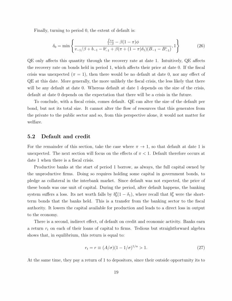
Finally, turning to period 0, the extent of default is:

δ0 = min

{f+s1−β − β(1− π)φ

v−1/β + b−1 − bc−1 + β(π + (1− π)δ1)(B−1 −Bc−1)

, 1

}(26)

QE only affects this quantity through the recovery rate at date 1. Intuitively, QE affects

the recovery rate on bonds held in period 1, which affects their price at date 0. If the fiscal

crisis was unexpected (π = 1), then there would be no default at date 0, nor any effect of

QE at this date. More generally, the more unlikely the fiscal crisis, the less likely that there

will be any default at date 0. Whereas default at date 1 depends on the size of the crisis,

default at date 0 depends on the expectation that there will be a crisis in the future.

To conclude, with a fiscal crisis, comes default. QE can alter the size of the default per

bond, but not its total size. It cannot alter the flow of resources that this generates from

the private to the public sector and so, from this perspective alone, it would not matter for

welfare.

5.2 Default and credit

For the remainder of this section, take the case where π → 1, so that default at date 1 is

unexpected. The next section will focus on the effects of π < 1. Default therefore occurs at

date 1 when there is a fiscal crisis.

Productive banks at the start of period 1 borrow, as always, the full capital owned by

the unproductive firms. Doing so requires holding some capital in government bonds, to

pledge as collateral in the interbank market. Since default was not expected, the price of

these bonds was one unit of capital. During the period, after default happens, the banking

system suffers a loss. Its net worth falls by bp0(1 − δ1), where recall that bp0 were the short-

term bonds that the banks held. This is a transfer from the banking sector to the fiscal

authority. It lowers the capital available for production and leads to a direct loss in output

to the economy.

There is a second, indirect effect, of default on credit and economic activity. Banks earn

a return rt on each of their loans of capital to firms. Tedious but straightforward algebra

shows that, in equilibrium, this return is equal to:

rt = r ≡ (A/σ)(1− 1/σ)1/α > 1. (27)

At the same time, they pay a return of 1 to depositors, since their outside opportunity its to

19

consume the capital. Therefore, banks would like to borrow all of the capital from depositors.

However, banks could run with the projects instead of repaying depositors. The incentive

constraint on this behavior gives a upper bound on the deposits the bank is able to attract:

ht ≤(

γ(1 + r)

1− γ(1 + r)

)[ωκt − bpt−1(1− δt)]. (28)

In between square brackets is the net worth of the banking system. This is what banks can

pledge to depositors, and this “skin-in-the-game” constrains the amount of lending they can

make. Defaults, by leading to losses to banks, lower their net worth, which tightens the

financial constraint and prevents them from raising deposits from households.

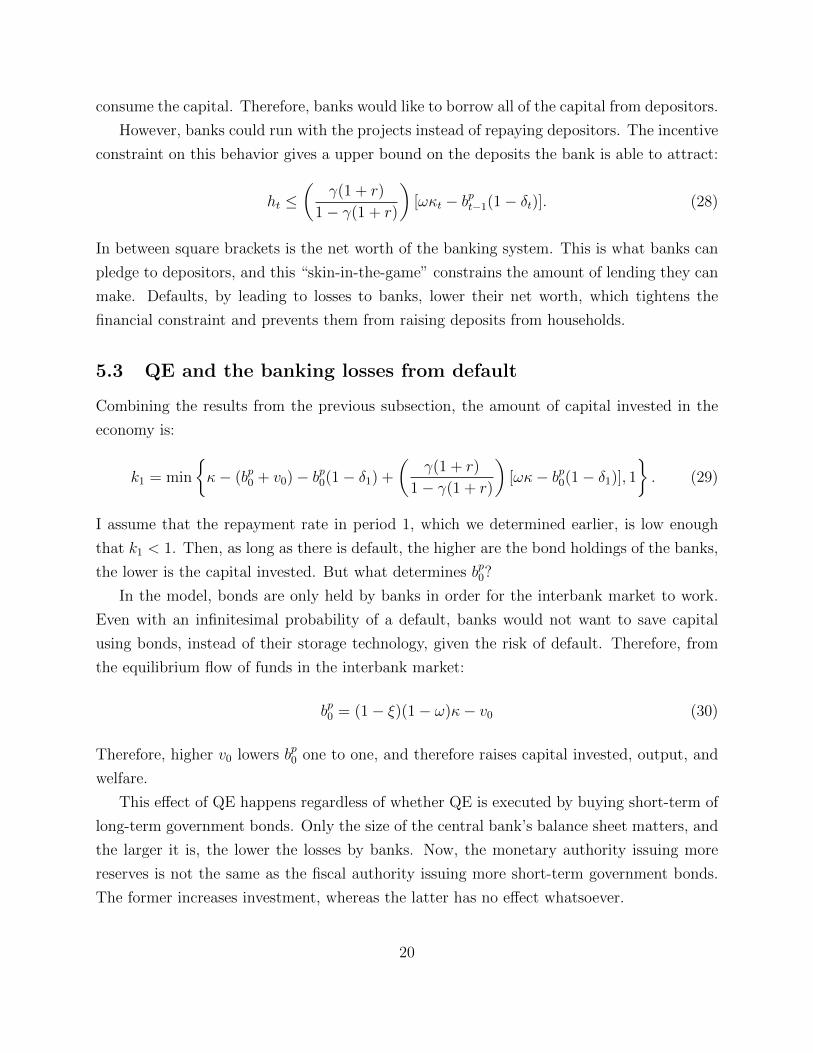
5.3 QE and the banking losses from default

Combining the results from the previous subsection, the amount of capital invested in the

economy is:

k1 = min

{κ− (bp0 + v0)− bp0(1− δ1) +

(γ(1 + r)

1− γ(1 + r)

)[ωκ− bp0(1− δ1)], 1

}. (29)

I assume that the repayment rate in period 1, which we determined earlier, is low enough

that k1 < 1. Then, as long as there is default, the higher are the bond holdings of the banks,

the lower is the capital invested. But what determines bp0?

In the model, bonds are only held by banks in order for the interbank market to work.

Even with an infinitesimal probability of a default, banks would not want to save capital

using bonds, instead of their storage technology, given the risk of default. Therefore, from

the equilibrium flow of funds in the interbank market:

bp0 = (1− ξ)(1− ω)κ− v0 (30)

Therefore, higher v0 lowers bp0 one to one, and therefore raises capital invested, output, and

welfare.

This effect of QE happens regardless of whether QE is executed by buying short-term of

long-term government bonds. Only the size of the central bank’s balance sheet matters, and

the larger it is, the lower the losses by banks. Now, the monetary authority issuing more

reserves is not the same as the fiscal authority issuing more short-term government bonds.

The former increases investment, whereas the latter has no effect whatsoever.

20

The special power of QE comes from the fact that reserves are held by the banking sector.

They cannot be traded for anything else so, by market clearing, an increase in the supply

of reserves must come with a one-to-one increase in reserve holdings by banks. Instead, an

increase in the supply of government bonds just comes with more holdings of government

bonds by the households. Banks, in the model, choose to buy the bonds after households

have cleared the market at the end of the period and will only buy the amount given in

equation (30). As long as b0 > (1− ξ)(1− ω)κ− v0, the household is the marginal holder of

government bonds so changes in bond supply gave no effect on banks.

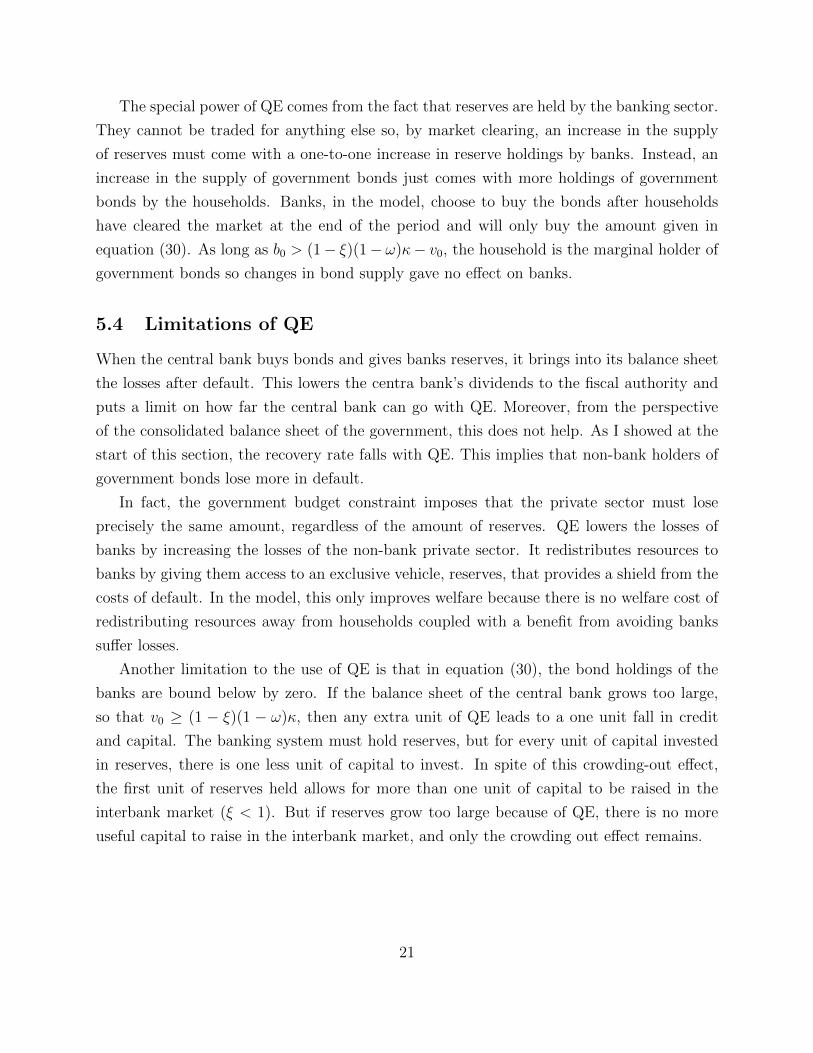
5.4 Limitations of QE

When the central bank buys bonds and gives banks reserves, it brings into its balance sheet

the losses after default. This lowers the centra bank’s dividends to the fiscal authority and

puts a limit on how far the central bank can go with QE. Moreover, from the perspective

of the consolidated balance sheet of the government, this does not help. As I showed at the

start of this section, the recovery rate falls with QE. This implies that non-bank holders of

government bonds lose more in default.

In fact, the government budget constraint imposes that the private sector must lose

precisely the same amount, regardless of the amount of reserves. QE lowers the losses of

banks by increasing the losses of the non-bank private sector. It redistributes resources to

banks by giving them access to an exclusive vehicle, reserves, that provides a shield from the

costs of default. In the model, this only improves welfare because there is no welfare cost of

redistributing resources away from households coupled with a benefit from avoiding banks

suffer losses.

Another limitation to the use of QE is that in equation (30), the bond holdings of the

banks are bound below by zero. If the balance sheet of the central bank grows too large,

so that v0 ≥ (1 − ξ)(1 − ω)κ, then any extra unit of QE leads to a one unit fall in credit

and capital. The banking system must hold reserves, but for every unit of capital invested

in reserves, there is one less unit of capital to invest. In spite of this crowding-out effect,

the first unit of reserves held allows for more than one unit of capital to be raised in the

interbank market (ξ < 1). But if reserves grow too large because of QE, there is no more

useful capital to raise in the interbank market, and only the crowding out effect remains.

21

6 QE and the ex ante costs of default

This section continues to study on the consequences of default while keeping prices stable.

Yet, while the previous section focussed on the size of default, captured in parameter φ, in

this section it is π, the probability of a fiscal crisis, that plays the center role. While in

the previous section the relevant constraint was on deposits, now it is the one on interbank

markets that will bind.

6.1 The interbank market

At date 1, banks’s borrowing in the interbank market is constrained by:

x1 =E0(δ1)bp0 + v0

1− ξ. (31)

The constraint binds when the fiscal crisis is sufficiently serious.

The price of bonds is given by their expected repayment rate. If there is no fiscal crisis,

repayment is 100%. But, if there is a fiscal crisis, equation (25) derived a formula for δ1

that is decreasing with the size of the fiscal shortfall. In turn, the lower is π the higher the

probability of a haircut. Therefore, a more serious crisis, understood as higher φ and lower

π, will both lower the price of bonds in the interbank market.

The result of this lower price is that banks have to buy more bonds bp0 in order to

collateralize the same amount of borrowing in the interbank market. As shown in the previous

section, this will imply that, if the fiscal crisis materializes at date 1, the losses of bank net

worth and the contraction in deposits and credit will be larger. There is an additional

channel through which a more likely crisis alone, or a lower E0(δ1) for a given δ1, has an

impact on investment and welfare.

6.2 Safe assets and market freezes

The amount of bonds that banks can purchase to use in the interbank market is bound

above by the amount of government bonds available: bp0 ≤ b0. While in normal times this

constraint will be very far from binding, when there is a deep crisis, it just might. In 2008,

during a financial crisis that we might interpret as a lower ξ, so the collateral requirements

in financial markets were higher, some argue that there were not enough safe assets around

to serve as collateral (Gorton, 2010; Caballero and Farhi, 2014).

22

In a fiscal crisis, this is an even more likely scenario. The crisis implies that government

bonds are no longer safe. In the model in this paper, agents care about expected payoffs

instead of Knightian uncertainty, so the possibility of default in government bonds does not

lead to a dramatic fall in the safe assets available. But, if the probability of a crisis is large

enough, and the fiscal shortfall is deep enough, the market value of government bonds may

not be large enough to sustain the functioning of the financial system. In this case, equation

(31) becomes:

x1 =E0(δ1)b0 + v0

1− ξ. (32)

QE can make up for the shortfall. While issuing reserves to buy short-term bonds would

make no difference, QE that buys long-term bonds relaxes the constraint. More reserves

allow for more financial transactions to take place between financial intermediaries, which in

turn allows more capital to be allocated to those that have good investment opportunities.

This boosts credit, investment, output and welfare.

6.3 Limitations of QE at providing safety

This model of safety is simple and stark. But it captures the basic insight that, in terms

of the safe assets that banks can hold, reserves will take a special place. They are are both

default-free, as well as held by the banking system entirely.

While in the model maturity is tightly linked to safety—only short-term bonds can be

used as collateral—all that matters is that the central bank can use QE to buy some assets

that are safe and others that are risky. The composition of the central bank’s balance sheet,

in this case in the split between the riskiness of different assets, will affect the amount of

safe assets available in the economy, which may allow financial markets to keep functioning

during a fiscal crisis. Insofar as it is hard to measure which assets are safe or not, many

forms of QE may turn out to be ineffective, just as purchases of short-term bonds were in

the model.

7 Discussion of some of the assumptions

The goal of this paper was to emphasize the possibilities for QE to have an effect, and it tried

to do so in a simple and transparent framework. Some of the assumptions, especially those

23

about the real environment, were inessential to the main results, while those that applied to

the actions of the monetary and fiscal authorities played a larger role.

7.1 Restrictive assumptions on the environment

The model simplifies the dynamics in three important ways.

First, nominal rigidities last only for one period. Therefore, the effects of both the fiscal

crisis and QE on unexpected inflation happen only in one period, instead of spreading over

time. Still, beyond propagation, more delayed price adjustments would not add to the

economic mechanisms at play.

Second, banks do not accumulate net worth over time, but exist for only one period.8

Therefore, shocks to bank equity due to default again do not propagate over time, and the

effects of QE are constrained to one period.

Third, there are only shocks in period 1. Generalizing this would still lead to the con-

clusions that QE can only affect unexpected inflation and that the bank equity channel is

due to surprises, while the safety channel is driven by expected defaults. Of course, to make

quantitative predictions on the effect of QE, it would be important to accurately capture

these dynamics.

Another assumption that plays little role is that only short-term bonds are used in inter-

bank markets and so these are the only bonds held by banks. For the bank equity channel

this played little role: changing the collateral constraint to include also long-term bonds

would have little effect on the conclusions. All that would matter for the effectiveness of

QE would be the size of the central bank balance sheet, not its composition. For the safety

channel, as long as the demand for safe assets by banks exhaust all of the government bonds

available that can fulfill this role, and that there are other assets that QE can buy so that

it can on net create safe assets by issuing reserves, the same results would hold.

7.2 Restrictive assumptions on policy

More important to the results are the interactions between QE and the other policies. With

respect to interest-rate policy, I assumed throughout that the monetary authority targeted

the price level. It is well known that this is optimal in sticky-information models, and under

8A related, inessential assumption, was that banks bought bonds at the start of the period, rather thanin the previous period. This was unimportant, since with one-period lived banks, the price of bonds wasEt−1(δt), while with multi=period lived banks and bonds bought the previous period, the price of the bondwould have been qt−1 = β Et−1(δt), so the exact same effects would be present.

24

a wide set of models and cases (Ball, Mankiw, and Reis, 2005; Reis, 2013). This matters

insofar as it affects how inflation surprises propagate over time and thus change the value of

bonds of different maturities. At an extreme example, if the monetary authority keep the

nominal interest rate fixed over time, say by it = β, then following a shock to the price level

due to a fiscal crisis, the price level would be permanently higher. But then, the value of

bonds of all maturities would fall by exactly the same proportional amount. QE would be

neutral because the maturity composition of the publicly held debt would be irrelevant for

the extent of debt debasement due to inflation. Outside of this knife-edge case, QE will have

the effects described in the text. Generally, the interest-rate policy followed by the central

bank will affect in what direction QE should be conducted.

The debt management of the fiscal authorities (bt, Bt) was taken as given. Yet, it might

respond to QE, and in the limit neutralize its effects. For instance, when the Federal Reserve

extended the maturity of its bond portfolio, the Federal Reserve increased the maturity of

its new issuances (Greenwood, Hanson, Rudolph, and Summers, 2014) partly offsetting QE.

Deciding who moves first in the game between fiscal and monetary authorities will play an

important role on the effectiveness of QE.

Finally, in the model in this paper, all government bonds were held domestically. There-

fore, from the perspective of the national economy, there was no benefit in defaulting, and

so government default only happened when it was inevitable. If some of the bonds were held

abroad, then the government might voluntarily choose to default, but in turn this would

affect the interest paid on the public debt. QE would determine not only the total amount

of government bonds outstanding, but also potentially how many are held abroad and their

maturity, affecting the relative benefits and costs of sovereign default as well as the ability

to commit to policies (e.g., Aguiar and Amador, 2014).

8 Conclusion

This paper put forward arguments for why quantitative easing can be a tool for the future

in central banking. While QE may have been neutral in the past, in a future where fiscal

crisis are possible, and perhaps long lasting, QE can play three roles. First, it can allow the

central bank to stabilize inflation by managing the sensitivity of inflation to fiscal shocks.

Second, it can lower the losses suffered by banks during a default and so stabilize credit

and investment. Third, it can provide safe assets when financial markets need them, and so

promote financial stability. All of these goals are consistent with the traditional objectives of

25

central banking. This paper described how managing the size and composition of the central

bank’s balance sheet could exploit these channels to achieve better outcomes.

For each of these roles, I also emphasized at least one limitation of QE. The central bank

is constrained in the management of its balance sheet by the risks to its own solvency, by

the redistribution between banks and the rest of the economy that it induces, and by the

potential to oversupply reserves and crowd out credit. Perhaps the largest limitation will be

how the fiscal authorities change their default and debt management policies in response to

QE. Studying the optimal use of QE, that takes into account both their benefits and costs

is an exciting question for future research to pursue.

26

References

Aguiar, M., and M. Amador (2014): “Take the Short Route: How to Repay and Re-structure Sovereign Debt with Multiple Maturities,” Princeton University manuscript.

Ball, L., N. G. Mankiw, and R. Reis (2005): “Monetary Policy for InattentiveEconomies,” Journal of Monetary Economics, 52(4), 703–725.

Balloch, C. M. (2015): “Default, Commitment, and Domestic Bank Holdings of SovereignDebt,” Columbia University manuscript.

Bernanke, B. S. (2015): The Federal Reserve and the Financial Crisis, no. 9928-2 inEconomics Books. Princeton University Press.

Bernanke, B. S., and V. R. Reinhart (2004): “Conducting Monetary Policy at VeryLow Short-Term Interest Rates,” American Economic Review, 94(2), 85–90.

Bolton, P., and O. Jeanne (2011): “Sovereign Default Risk and Bank Fragility in Fi-nancially Integrated Economies,” IMF Economic Review, 59(2), 162–194.

Caballero, R. J., and E. Farhi (2014): “The Safety Trap,” NBER Working Papers19927, National Bureau of Economic Research, Inc.

Chen, H., V. Curdia, and A. Ferrero (2012): “The Macroeconomic Effects ofLargescale Asset Purchase Programmes,” Economic Journal, 122(564), F289–F315.

Cochrane, J. H. (2001): “Long-Term Debt and Optimal Policy in the Fiscal Theory ofthe Price Level,” Econometrica, 69(1), 69–116.

Cochrane, J. H. (2014): “Monetary policy with interest on reserves,” Journal of EconomicDynamics and Control, 49(C), 74–108.

Corhay, A., H. Kung, and G. Morales (2014): “Government Maturity Twists,” Lon-don Business School.

Eggertsson, G. B., and M. Woodford (2003): “The Zero Bound on Interest Rates andOptimal Monetary Policy,” Brookings Papers on Economic Activity, 34(2003-1), 139–235.

Gertler, M., and P. Karadi (2013): “QE 1 vs. 2 vs. 3. . . : A Framework for AnalyzingLarge-Scale Asset Purchases as a Monetary Policy Tool,” International Journal of CentralBanking, 9(1), 5–53.

Gertler, M., and N. Kiyotaki (2010): “Financial Intermediation and Credit Policy inBusiness Cycle Analysis,” in Handbook of Monetary Economics, ed. by B. M. Friedman,and M. Woodford, vol. 3 of Handbook of Monetary Economics, chap. 11, pp. 547–599.Elsevier.

Gorton, G. B. (2010): Slapped by the Invisible Hand: The Panic of 2007, no.9780199734153 in OUP Catalogue. Oxford University Press.

Greenwood, R., S. G. Hanson, J. S. Rudolph, and L. Summers (2014): “Govern-ment Debt Management at the Zero Lower Bound,” Hutchins Center Working Paper No.5.

27

Hilscher, J., A. Raviv, and R. Reis (2014a): “Inflating Away the Public Debt? AnEmpirical Assessment,” NBER Working Paper 20339.

(2014b): “Measuring the Market Value of Central Bank Capital,” Brandeis Uni-versity and Columbia University.

Krishnamurthy, A., and A. Vissing-Jorgensen (2011): “The Effects of QuantitativeEasing on Interest Rates: Channels and Implications for Policy,” Brookings Papers onEconomic Activity, 43(2 (Fall)), 215–287.

Morais, B., J. L. Peydro, and C. Ruiz (2015): “The International Bank LendingChannel of Monetary Policy Rates and QE: Credit Supply, Reach-for-Yield, and RealEffects,” International Finance Discussion Papers 1137, Board of Governors of the FederalReserve System (U.S.).

Perez, D. (2015): “Sovereign Debt, Domestic Banks and the Provision of Public Liquidity,”Stanford University manuscript.

Reis, R. (2009): “Interpreting the Unconventional U.S. Monetary Policy of 2007-09,” Brook-ings Papers on Economic Activity, 40, 119–165.

(2013): “Central Bank Design,” Journal of Economic Perspectives, 27(4), 17–44.

(2015): “Different types of central bank solvency and the central role of seignorage,”Columbia University.

Sargent, T. J. (1982): “The Ends of Four Big Inflations,” in Inflation: Causes and Effects,NBER Chapters, pp. 41–98. National Bureau of Economic Research, Inc.

Uribe, M. (2006): “A fiscal theory of sovereign risk,” Journal of Monetary Economics,53(8), 1857–1875.

Vayanos, D., and J.-L. Vila (2009): “A Preferred-Habitat Model of the Term Structureof Interest Rates,” CEPR Discussion Papers 7547, C.E.P.R. Discussion Papers.

Wallace, N. (1981): “A Modigliani-Miller Theorem for Open-Market Operations,” Amer-ican Economic Review, 71(3), 267–74.

Woodford, M. (2003): Interest and prices: foundations of a theory of monetary policy.Princeton University Press.

28