qa 101: pm qa requirements - us epa 101: pm qa requirements round robins: lab bias & pm 2.5 pep:...
TRANSCRIPT

QA 101: PM QA Requirements
PM2.5 PEP: Network BIASRound Robins: Lab Bias & Accuracy
8/8/2016 2016 National Air Monitoring Conference 1

Session Overview
8/8/2016 2016 National Air Monitoring Conference 2
• ID important Regs and
Guidance that pertain to QA Network
Site & Sampler
Lab
Data Management
• Spend some time looking at
some of the QA elements that
can help you assess and
optimize network data quality

Session Overview
8/8/2016 2016 National Air Monitoring Conference 3
What do I Need to “Get” from
the PM QA 101 Session ….?1. Understand Data Quality Objectives and
Measurement Quality Objectives for PM2.5 and PM10
monitoring
2. Understand the measurements that are made to
quantify or otherwise gauge our achievement of
these objectives
3. Understand what the results of the measurements
or assessments tell me about my sites, my lab, my
network and my monitoring data

Reg Requirements
8/8/2016 2016 National Air Monitoring Conference 4
40 CFR Part 50 FRMs—
samplers and labs
a. Appendix B: Hi volume
samplers
b. Appendix J: PM10
c. Appendix L: PM2.5 & PM10 (Low
volume)
40 CFR Part 53 FEMs—
samplers and labs
a. FEM performance specifications;
b. Testing requirements, and c. Approval designations

Reg RequirementsCont.
8/8/2016 2016 National Air Monitoring Conference 5
40 CFR Part 58
• Appendix C: Monitoring
Methodology; ARM alternatives
to FRM/FEM; exceptions and
waivers

More Reg Requirements??
40 CFR Part 58
• Appendix D Network Design:a. Monitoring objectives
b. Network Scale Objectives (pollutant specific)
i. Microscale
ii. Middle Scale
iii. Neighborhood
iv. Urban
v. Regional
c. Site Classifications based
on data usage, e.g.,
SLAMS, NCORE
8/8/2016 2016 National Air Monitoring Conference 6
Criteria
Established by
Monitoring Plan
and QAPP

40 CFR Part 58
Appendix E: Monitoring Path Siting Criteria for Ambient Air Quality Monitoring
► Horizontal and Vertical Placement of
inlets
► Spacing from Minor Sources.
► Spacing From Obstructions.
► Spacing From Trees
► Spacing From Roadways.
8/8/2016 2016 National Air Monitoring Conference 7

8/8/2016 2016 National Air Monitoring Conference 8
Slide 7 All these are important Quality factors, which should be used whenever you are assessing site capability. Some
are again very important to clean air demonstrations. For example, overgrown trees and construction of large buildings
subsequent to the initial start-up of the samplers could end up invalidating entire years worth of data. TSAs are designed to
identify these kinds of issues before they become critical. Horizontal and vertical placement of monitor inlets is very
important in designing sites to enable QA assessments. Note the April 2016 provides opportunity for more flexibility with
the advent of the FEMs. The Appendix A discussion will have more to say about inlet positions.
The next couple of slides illustrate some typical findings during TSAs at some sites. Slide 9 Inlet to close to Parapet, but new regs allow for a waiver. Even if the TSP sampler on the right is a Pb sampler. This source could create enough soot on the filter in some instances to dramatically affect the flow rate and created error in the calculated concentration
Slide 10 On the left there is much to much shrubbery and growth. It will continue to get worse unless it is cleared. The deck on the right takes near road sampling to a new level. It may still be ok if the vehicles per day count is below the threshold.

8/08/2016 2016 National Air Monitoring Conference 9
Courtesy of Laura Niles, CARB
Courtesy of
Richard Guillot,
EPA Region 4
Source too close
to TSP Sampler

8/11/2014 2014 National Air Monitoring Conference 10
Courtesy of Florida DEP
Courtesy of Thien
Bui, EPA Region 8

Then there’s Guidance!!
8/8/2016 2016 National Air Monitoring Conference 11
• Guidance Referenced by Regs
1. QA Handbook Volume II, Appendix D is the “Rosetta Stone” for QA measurement requirements.
a. https://www3.epa.gov/ttn/amtic/files/ambient/
pm25/qa/QA-Handbook-Vol-II.pdf and
b. https://www3.epa.gov/ttn/amtic/pmqa.html2. Quality Assurance Guidance
Document 2.12: Monitoring PM2.5 in Ambient Air Using Designated Reference or Class I Equivalent Methods
https://www3.epa.gov/ttn/amtic/files/ambient/p
m25/qa/m212.pdf
3. Document 2.11 covers PM10(1990 !!)

8/8/2016 2016 National Air Monitoring Conference 12
Slide 11 Ya gotta know how to get to these documents,--especially 1 & 2. Notice AMTIC is in the URL. The great thing
about the templates is that they are 1-stop shopping for DQOs MQOs and other critical criteria. The current validation
tables in the Vol II URL (1.a.) contains the PM 10 requirements. The second URL (1.b.) is a recent update to the PM2.5
validation template. Document 2.12 was revised earlier this year. Notice that the PM-10 guidance (document 2.11) is very
dated. The entire Vol. II and the complete template are currently undergoing review and revision by the EPA Regional and
SLT QA workgroup. It will incorporated the recent changes to PM2.5. A schedule has not been set to revise Document
2.11. By the way, this entire unabridged presentation will be in the national ambient air monitoring conference
compendium---on AMTIC.

8/8/2016 2016 National Air Monitoring Conference 13
1. Assessing Monitor Performance a. NIST traceable Standards
b. Flow rate verifications
c. Flow rate audits
2. Network: Data Quality Objectives:
a. Collocation and Precision
measurements, then
b. Bias
3. Laboratory QA/QC elementsa. Environmental Conditions
b. Analytical Equipment
c. Routine QC Data Acquisition

8/8/2016 2016 National Air Monitoring Conference 14
"Traceable" is defined in 40 CFR
Parts 50 and 58 as meaning that “a
local [field or transfer] standard has
been compared and certified either
directly [with] or via not more than
one intermediate standard [one level
from], [to] a primary standard such as
a National Bureau of Standards
Standard Reference Material (NBS
SRM), or a USEPA/NBS-approved
Certified Reference Material (CRM).”
40 CFR Part 58, Appendix A Sections 3.2.1, 3.2.2, 3.3.1 and 3.3.3: Flow
rate standards must be NIST-traceable

8/8/2016 2016 National Air Monitoring Conference 15
• 40 CFR Part 50, Appendix L Sec 9.1 & 9.2
• Verification, calibration and audit
(“working”) standards should be “re-
calibrated or re-verified at least annually”
• Traceable to a NIST “Primary Standard”
What if I cannot send my 6 ± working standards
to an independent Metrology Lab?

8/8/2016 2016 National Air Monitoring Conference 16
At a minimum, the “certification procedure” for a working
(or “transfer”) standard should:
• Find a NIST Traceable Primary standard—the Region,
your own lab, a corporate lab
• Establish the parametric range of the working standard
relative to the primary (Stationary Bench) standard;
• Certify that the primary standard (and hence the
working standard) is traceable to a NIST primary
standard; (It should have a certificate!)
• Include a test of the stability of the working standard
over several days and test repetitions; and
• Specify a recertification interval (i.e. 365 days) for the
working standard
• All this should be in an SOP and your QAPP!

8/8/2016 2016 National Air Monitoring Conference 17
For Hi Vol PM-10

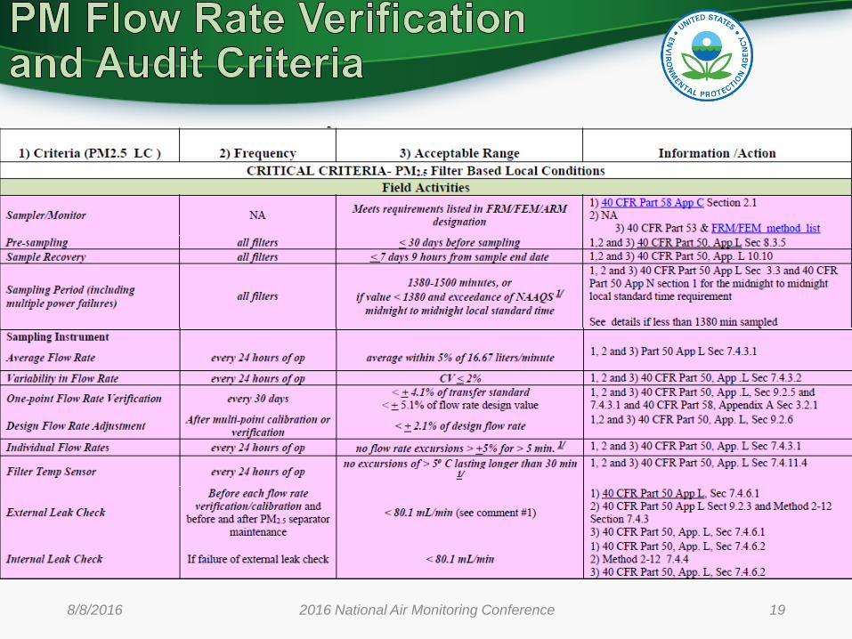
8/8/2016 2016 National Air Monitoring Conference 18
• Verificationsi. PM2.5 & LoVol PM10-Monthly
(minimum 14 days apart) ii. HiVol PM10 -Quarterlyiii. Look at Avg Flow CV for
each event
• Report PM2.5
and PM10
Verifications to AQS!!
• Flow Audits 2X+ per yearBy “Independent Auditors” or
at least with independent, NIST-traceable standards
5 to 7 months apart
A tribute to George Froelich
40 CFR Part 58 appendix A
Sections 3.2.1, 3.2.2, 3.3.1 and 3.3.3
8/8/2016 2016 National Air Monitoring Conference 19

You might ask “Why
are these important?”
8/8/2016 2016 National Air Monitoring Conference 20
• In addition to detecting failures, indicates
sources of bias or relatively inaccuracy—
Might actually save some data!!
The cut point of the PM separators (size of the particles
collected) are dependent on the flow rate
The final concentration value derived from filter based
measurement is mass gained on the filter divided by the
sample volume, i.e., = mass /(24 hours X flow rate)

8/8/2016 2016 National Air Monitoring Conference 21
• Keeping your flow rates within acceptance limits is crucial, especially if ambient concentrations at the site in question might occasionally approach the standard. The reason is that the relationship between flow rate, cut-point of the PM separator are not linear. Outside of the flow rate acceptance limits of the FRM, the effects of PMcoarse (PM10-2.5) can be counterintuitive.
• Let’s use example the depicted on the VSCC Cyclone curve. Suppose your sampler is telling you the flow is 16.7 lpm but it is really 14.0 lpm. Under ordinary circumstances you would invalidate the data if you discovered this operational anomaly. Without an awareness of the anomalous flow rate an agency can be accepting data that is pretty far from reality and they could be drawing erroneous conclusions about the design value for the affected area. This particular cut point curve, happens to be for the MESA Lab’s BGI PQ200 FRM Sampler with a VSCCB, but the principle would be true for all the VSCCs. Notice that at 14.0 lpm you are collecting some PM-3 and smaller. Suppose the lab measures 221.8 µg of PM mass collected on the filter. To actually estimate the real PM2.5 your would need to independently assess the mass of the PMcoarse fraction PM3-2.5 that is also collected by the sampler, i.e., fraction of the 221.8 µg PM mass that was collected. This would take some rather sophisticated and expensive non-FRM measurements.
• For illustration lets assume the concentration of PM3-2.5 is 4 µ/m3.
• If you do not account for the PM3-2.5, you might simply correct for the flow rate with the second equation, which would push your apparent PM2.5 toward the annual NAAQS. However, if you know the real concentration of PM3-2.5, which as assumed in this case, was 4 µ/m3, the last equation shows that the apparent PM2.5 concentration is significantly higher than the realconcentration. In other words in this example, we significantly over estimated the PM2.5.by nearly a factor of 2!!

Lpm D50 Kenny Data
2 19.768 18 2.36
4 10.057 15 2.758
6 6.773 11.4 3.57
8 5.116 15.7 2.66
10 4.116 18.7 2.295
12 3.446
14 2.965 Work Area
16 2.603 Q D50
18 2.32 45 1.04
20 2.094
D50= 2.50
Lpm= 16.67 d50 = 31.48Q-0.8963
0
0.5
1
1.5
2
2.5
3
3.5
4
4.5
5
10 12 14 16 18 20
D50
Lpm
VSCC - 2.946
Effect of flow on cut point of particle size
Courtesy of MESA Labs. (BGI Inc)

But what if the concentration of PM3-2.5 is 4 µg/m3 or 96.0 µg/filter, as
independently measured!! By having a real flow rate that is lower
than what the sampler told you, your apparent concentration was
nearly twice the real PM2.5 Concentration!
C app = 221.8 µ/filter X 1 filter/event X 1000 liters/m3
X 60 min/hr X 24 hr/event
C ind = 221.8 µ/filter X 1 filter/event X 1000 liters/m3
X 60 min/hr X 24 hr/event
14.0 liters/min
16.7liters/min
8/8/2016 2016 National Air Monitoring Conference 23
Effect of Flow on Concentration Value-a hypothetical caseLab measures
Sampler
Reports
Flow standard
Reports
= 9.2 µg/m3
= 11.0 µg/m3
Creal = Capp X (221.8 – 96.0) = 6.3 µg/m3
221.8

The Example in this presentation was based on a PM2.5 sampler fitted with VSCC but the same
principles is true for the WINS. In fact, there has been some research performed, early in the life of
the network, on bias introduced by flow rates outside the design acceptance limits. The publication
citation for this report is below.:
Robert W. Vanderpool, Thomas M. Peters, Sanjay Natarajan, Michael P. Tolocka , David B. Gemmill & Russell W. Wiener (2001) Sensitivity Analysis of the USEPA WINS PM2.5 Separator, Aerosol Science and Technology, 34:5, 465-476, DOI: 10.1080/02786820120868
8/11/2014 2014 National Air Monitoring Conference 24
Within flow rate acceptance limits of the (FRM ± 4% of the design flow rate) the contribution of
PMcoarse will be less dramatic, and in fact, maybe not distinguishable. In this case, as was also
shown in the WINS study below. The loss of flow below the design value vs gain in extra mass
above PM2.5; or the loss of PM2.5 when flow rate is above the design value vs increased flow
volume times the PM2.5 that is collected are considered to be offsetting factors
The Bottom Line: Conduct your flow verifications and audits
and report them AQS!!

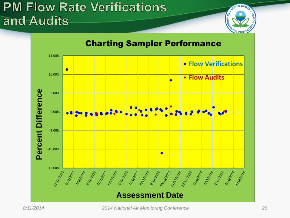
What are some cool and useful things you can do with verification data? What about a rather simple method of tracking sampler performance shown in the next slide(#26). Since audits occur only every 6 months if an audit reveals a malfunction, verifications can reveal how far the back the data must be rejected. In this example you can see it looks like corrections were made on the spot after verifications suggested the samplers went out of spec.
You can also use the event flow CVs (in the second slide #27) that are reported by the sampler to spot trouble and check out conditions before a crisis emerges. In this case the erratic behavior in several sampling events during September and October 2013 suggested someone should do a little trouble shooting—maybe the pump; maybe the power supply to the sampler.
8/11/2014 2014 National Air Monitoring Conference 25
8/11/2014 2014 National Air Monitoring Conference 26
-15.00%
-10.00%
-5.00%
0.00%
5.00%
10.00%
15.00%
Pe
rce
nt
Dif
fere
nc
e
Assessment Date
Charting Sampler Performance
Flow Verifications
Flow Audits

8/8/2016 2016 National Air Monitoring Conference 27
0.0%
0.5%
1.0%
1.5%
2.0%
2.5%
3.0%
3.5%
Sample Run Date
Daily Avg Flow CV

8/8/2016 2016 National Air Monitoring Conference 28

• 40 CFR Part 58 Appendix A
2.3.1.1 Measurement Uncertainty for Automated and Manual PM2.5 Methods.
10 % CV for total precision, and
±10 % difference for total bias.
8/8/2016 2016 National Air Monitoring Conference 29
Data Quality Objectives
for PM2.5
Aggregated over 3** year at the National level!
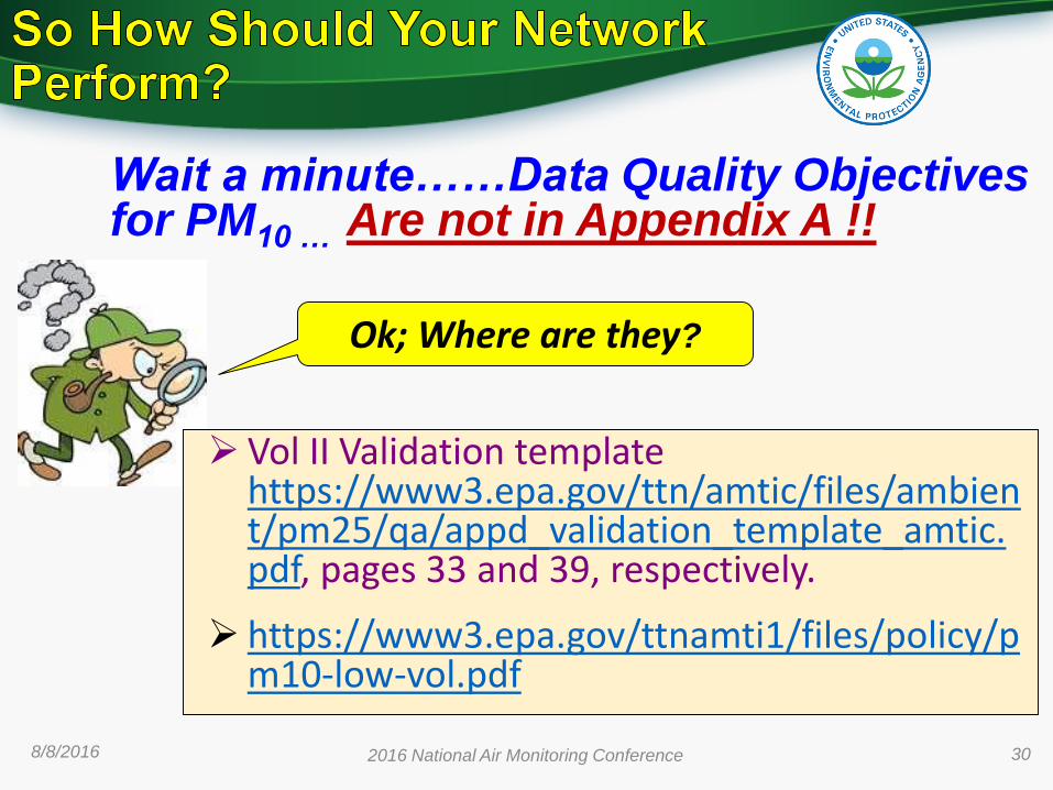
Vol II Validation template https://www3.epa.gov/ttn/amtic/files/ambient/pm25/qa/appd_validation_template_amtic.pdf, pages 33 and 39, respectively.
https://www3.epa.gov/ttnamti1/files/policy/pm10-low-vol.pdf
8/8/2016 2016 National Air Monitoring Conference 30
Wait a minute……Data Quality Objectives for PM10 … Are not in Appendix A !!
Ok; Where are they?

High volume Collocated Precision <10.1% CV for concentrations ≥ 15 µg/m3
No independent Bias value for High-volume PM-10
Low volume
Same as PM2.5 (per
8/8/2016 2016 National Air Monitoring Conference 31
Data Quality Objectives for PM10 (per “Volume II” Validation template)
Aggregated over 3 years** at the National level!

8/8/2016 2016 National Air Monitoring Conference 32
40 CFR Part 58 Appendix A
• Precision is derived from Agency-owned and operated collocated samplers
PM2.5: Section 3.2.3
PM10: Section 3.3.4
• Bias provided by “independent” FRM samplers collocated with Primary samplers
PM2.5: Section 3.2.4 Performance Evaluation Program (PEP), or
• Internal bias based on flow rate verifications for PM2.5 and Low–vol PM10: Sections 3.2.1 and 3.3.1

What happens When the Ambient Concentration Gets Small
• Collocated precision measurements and PEP bias measurements are considered valid for the applicable statistical algorithm, if:both the primary monitor and collocated sampler or PEP audit
concentrations are otherwise valid, and
Each is above a prescribed threshold given at…
40 CFR Part 58 Appendix A Section 4.(c).1) PM10 (Hi-Vol): 15 μg/m3.
2) PM10 (Lo-Vol): 3 μg/m3
3) PM2.5 and PM10–2.5: 3 μg/m3.
• AQS does not pair data from either event unless both concentrations are valid
• Also see 40 CFR Part 58 Appendix A Section 3.2.4
33

Any sampler placed beside a primary sampler for measurement or collection of data that can be related to the primary sampler
8/8/2016 2016 National Air Monitoring Conference 34
What is a Collocated
Sampler?

What is the primary sampler?
Sampler that produces ambient concentration data for determining compliance with NAAQS or other regulatory requirements
8/8/2016 2016 National Air Monitoring Conference 35
Appx A
3.2.3 & 3.3.4.1
There can be only
one primary PM25
or PM10 sampler
per site for a
specified period of
time.
∴Make sure your
primary sampler is
designated correctly in
AQS!!

#Primary FEMS
of each unique
method
designation
Collocations
Required
#Collocated
with an
FRM
#Collocated
with same
method
designation
1-9 1 1 0
10-16 2 1 1
17-23 3 2 1
24-29 4 2 2
3.2.3.1 General: For each distinct monitoring method designation (FRM or
FEM) that a PQAO is using for a primary monitor, the PQAO must have 15
percent of the primary monitors of each method designation collocated.
The First Collocated Monitor must be a FRM!!
We took some of the “guess work” out of the FEM collocations:

3.2.3.4 (a) and (b)--- 50% (of the 15%) locate at sites with
ambient concentrations within ± 20% NAAQS; If ambient
concentrations < 20% NAAQS, 50% at sites with highest
concentrations. Remaining 50% at SLT’s discretion.
3.2.3.4(c) Spatial requirements
i. samplers 1-4 meters apart horizontally;
ii. Rule clarification: EPA Waiver by Region can allow up
to 10 meters horizontally and up to 3 meters vertically
8/8/2016 2016 National Air Monitoring Conference 37

General: Applies to
15 percent of the primary monitors collocated.
Spatial deployment similar to PM2.5
Hi-vol TSP cannot be Surrogate Primary samplers for PM10
HI-vol samplers
PM10-2.5 Primary Sampler may also be a Primary PM10
Sampler; the method designation of the collocated sampler
has to match
Low-vol Pb and PM10 samplers may share a collocated
sampler, in which caseTotal PM10 Mass on the filter must be measured before chemical
analysis for Pb
manual (filter based) samplers only

8/11/2014 2014 National Air Monitoring Conference 39
From 40 CFR Part 58 Sections 4.1.1 & 4.1.2
In Equation 1, “d” is the percent difference of the primary sampler’s measured concentration,
“meas,” and the “audit” concentration of the collocated sampler. “i” is the single event in
which a primary monitor and the collocated monitor have acquired valid samples.
In Equation 2, “n” is the number of single point checks being aggregated; X20.1,n-1 is the 10th
percentile of a chi-squared distribution with n-1 degrees of freedom.

• Calculate and plot CV via the DASC tool Overall CV
FRM-FRM
FEM-FRM
FEM-FEM, if you have FEM-FEM collocations
• Primary vs collocated scatter plot showing outliers
• Plot of % difference FEM(s) vs FRM (the PM2.5 Bias equation gives an in-house bias Plot of Daily Bias over time using 1 point QC check
equation provides precision
8/8/2016 2016 National Air Monitoring Conference 40

41
Most data <± 10%; Avg-horizontal (bias) ≈ 0, slope slightly+
17 • Using 2008-
2010 precision
data,
consistent
differences
suggest bias in
one or both
samplers.
A trend in
differences
suggest a
progressive
bias in one
sampler.
Courtesy of Shelly Eberly

Can Precision Data Give Insights into Bias?
42
• Using 2008-2010
precision data,
• consistent
differences
suggest bias in
one or both
samplers.
• trends in
differences
suggest trends
in bias in one
or both
samplers.
Most data <± 10%; Avg. horizontal (bias) ≈ -4%; slope ≈ 0
17
Courtesy of Shelly Eberly
8/8/2016 2016 National Air Monitoring Conference

What do these indicate????43
Noisy precision with
possible upward
trend in bias.
Noisy precision with oscillations.
Larger positive relative differences in
summer, larger negative relative
differences in winter (Method Code170).
20
Courtesy of Shelly Eberly8/08/2016 2016 National Air Monitoring Conference 43

• Collocates an independent FRM audit sampler beside a FRM/FEM
• Provides independent assessment of network sampler bias
• Applies rigorous performance and QA/QC requirements to field and laboratory operations
• Might indicate if the monitoring agency’s FRM is experiencing performance issues, BUT
60 days after the fact!
Each measurement is only 1 data point for one isolated sampling event…..
8/8/2016 2016 National Air Monitoring Conference 44

• PEP Event Count for Each PQAO:• 15% of all sites audited per year; all sites in 6 years
• If 5 sites or less: 5 audits per year
• If >5 sites: 8 sites per year unless > 48 sites
• At least one of each “monitor type” audited each year
• FEMs and SPMS are included in the site count, unless classified as “excluded from design value determinations”
Speaker notes: We now perform about 600 Bias measurements per year The take away messages is that every
PQAO is not going to get very many data points in any given year. I even wonder about annual aggregation. You will see why this may be an growing issue in the following slides.
8/8/2016 2016 National Air Monitoring Conference 45

8/8/2016 2016 National Air Monitoring Conference 46
nj
Bias = -----1
njΣj =1
SLT - PEPPEP
j
where nj is the number of bias pairs
to be averaged. Note that this term
is “di” in Equation 1 of Appendix A.
SLT - PEPPEP
j
X 100%
From 40 CFR Part 58 Appendix A Sections 4.1.1 & 4.1.2
See the DASC tool at https://www3.epa.gov/ttn/amtic/files/ambient/qaqc/dascv3.xls

8/8/2016 2016 National Air Monitoring Conference 47
What does the PM2.5 data look like? Exactly what can it tell us. Slide 48 is a plot of one
agency’s annual bias data over several years and some precision data superimposed. We used
the bias equation for the precision data in this analysis to keep everything scaled similarly. We
have reported in past conferences the dramatic shift in bias during 2007-2009. Notice while the
difference between the bias and the precision seem dramatic the annual averages rise and fall in
the same direction from 2007 through 2010. And again note that the precision average is based
on about 30 data points 1 in 6 day sampling and the bias no more than 9 events annually, at
least after 2006. There are several factors that we have concluded contribute to this disparity
but also keep in mind that the math itself can over emphasize the difference. As the ambient
concentration measurements get smaller less than 10 µg/m3, the probability of creating a bias
value > ± 10% increases.
Slide 49 is a good example We know historically that the PEP values are a little higher than
the SLT values, so if the PEP sampler is off by no more than 1 µg/m3 (half of the method LDL)
from an SLT’s primary sampler on a given day, the bias can be easily skewed to unacceptable
values by the regulations. One or two PEP results like this can easily put the DQO out of reach
in a given year even though the actual difference between the PEP and SLT measurements are
1 µg/m3. keep in mind that the FRM LDL is 2 µg/m3.

Uses for PEP Bias data
8/8/2016 2016 National Air Monitoring Conference 48
-14
-12
-10
-8
-6
-4
-2
0
2
4
6
8
10
12
2000 2001 2002 2003 2004 2005 2006 2007 2008 2009 2010 2011
PEP
AGENCYPRECISION

8/8/2016 2016 National Air Monitoring Conference 49
SLT and PEP values of 4 and 5 µg/m3,
respectively, would yield a bias of -20%,etc.
The SLT sampler has produced a concentration
measurement of 5 µg/m3 and the PEP sampler 6
µg/m3. According to Equation 1:

Uses for PEP Bias dataSpeaker Notes
508/8/2016 2016 National Air Monitoring Conference
Slide 51 Here’s what has been happening the last 3 and a half years across the nation. Thankfully
the average has stabilized around – 7ug/m3. But there is still a lot of variability. You cannot tell
from this plot that the data set includes about 190 events in which either the PEP or the SLT value
was 3ug/m3 or less. When I extracted all of those values, the bias, SD and UCL/LCL changed to
the next graph.
Slide 52 Notice that there are still a lot of data points that fall considerably outside of the ± 10% (SD
= 15.2 %) even though the UCL/LCL values for the nation look pretty good. Do we know why there
are so many excursions? Its speculation at the moment, but I believe it is the higher variability
exhibited by the FEMs overlaid by the influence of lower concentrations. Why did I take out the
events at 3 µg/m3? Because the reg says so, and the AQS AMP 256 and AMP 600 reports, which
use the same statistical metric, also exclude them. Look at the following slide.
Slide 53 We have already seen what can happen to bias at values between 3 and 6 ug/m3. The 3
ug/m3 cut-off for data exclusion in the bias statistic poses a second dilemma. We have essentially
lost about 200 data pairs thus far since Jan 2013 due to the cut off, and the rate is increasing
rapidly. Since we only collect 5 or 8 PEP samples annually anyway, it is conceivable that the
confidence level utilized for development of the DQO may no longer adequately represent the bias
of an individual PQAO’s data set each year.

Uses for PEP Bias data
Jan 2013 - May 2016 National PM 2.5 Bias with data <3 µg/m3
Avg= -7.7 % ; SD = 16.7 %
51
Bias UCL (%) -7.04
Bias LCL (%) -8.40
8/8/2016 2016 National Air Monitoring Conference

Jan 2013 - May 2016 National PM 2.5 Bias with data >3 µg/m3
Uses for PEP Bias data
Avg= -6.7 % ; SD = 15.2 %
52
Bias UCL (%) -6.08
Bias LCL (%) -7.38
8/8/2016 2016 National Air Monitoring Conference

538/8/2016 2016 National Air Monitoring Conference

548/8/2016 2016 National Air Monitoring Conference
Slide 55 We have noticed an interesting characteristic of the data below the 3 ug/m3 threshold. In
all but a few instances the absolute difference between the PEP and SLT’s measured concentration
is 1 ug/m3 or less. This is half the FRM’s LDL. As a result we are now considering a change to the
Bias statistic. You will see in our PEP field blanks slide (#69) below that 1 ug/m3 is not an
unrealistic practical LDL for the PEP program at least. You may be able to establish a similar LDL
in which case a practical rationale for annually certifying your data may be apparent.

558/8/2016 2016 National Air Monitoring Conference

Four Areas of Control
• Lab Environment
• Analytical Equipment
• Analytical and QA/QC procedures
• Data Management
8/8/2016 2016 National Air Monitoring Conference 56
https://www3.epa.gov/ttn/amtic/files/ambient/pm25/qa/PM2.5_Val_Template_4_27_16.pdf

8/8/2016 2016 National Air Monitoring Conference 57
https://www3.epa.gov/ttn/amtic/files/ambient/pm25/qa/PM2.5_Val_Template_4_27_16.pdf

8/11/2014 2014 National Air Monitoring Conference 58

8/8/2016 2016 National Air Monitoring Conference 59
How Does one verify and document conformance?

8/8/2016 2016 National Air Monitoring Conference 60
Upper limit Standard Deviation Temperature
Limit =
21ºC ± 2.ºC
for the 24 hrs.
preceding
weighing
Session
SD (UL) =
2ºC over that
period

8/8/2016 2016 National Air Monitoring Conference 61
0
0.2
0.4
0.6
0.8
1
1.2
1.4
Daily %
RH
Std
.Dev
Weighing Date
Daily RH Standard Deviation
35
35.5
36
36.5
37
37.5
38
38.5
39
39.5
% R
ela
tive H
um
idit
y
Weighing Date
Relative Humidity ControlAvg RH between
30-40% for the
24 hrs.
preceding
weighing
Session. (in arid
region <5% of
RH during
sampling event).
Variability =
± 5 RH % of Avg
over that period
but >30% (arid
>20%)

8/8/2016 2016 National Air Monitoring Conference 62
31
32
33
34
35
36
37
38
39
% R
ela
tive H
um
idit
y
Date
Humidity Control
Redundant
monitoring
devices can
prevent pain, i.e.,
lost monitoring
data!!
In 2011 we lost a significant amount of PEP data because
the deployed logger was stuck on a single value and we
were not watching the control chart.

• Grounded Equipment
• Fresh Polonium 210 (more efficient)Center filters between strips positioned 2 inches apart
Give it time! Waving a filter between 2 strips for a half a second probably will not be adequate
• Additional equipment such as U-bars also improve the dissipation of electrons
• Test your procedure by charging, weighing and then reweighing filters. (hint: slide them in a petri across a counter top)
• Consult with the filter and balance venders.8/8/2016 2016 National Air Monitoring Conference 63

• Gravimetric balance: Vender maintenance and calibration—1/year
• ASTM Calibration Weights: NIST Certification—1/year
• ASTM Check Weights compare against Calibration weights—1/quarter
• Remember to Bracket the combined mass of the filter and expected PM filtrate 1-500 mg and 1-300 mg
8/8/2016 2016 National Air Monitoring Conference 64

LAB: Analytical QA/QCProcedures
• Internal and independent performance testing
Technician accuracy and precision
Bias between/among several Technicians
• ASTM/NIST-traceable Check and calibration weights
Monitor the condition and performance of the balance and the
weights
• Lab Blanks and Trip blanks, Batch and Inter-batch
duplicates
Indicates what is going on in the lab environment and the
filter handling process
• Field Blanks
Indicate level of contamination in lab and the field
8/8/2016 2016 National Air Monitoring Conference 65

LAB: Analytical QA/QCProcedures
• Internal and independent performance testing Technician accuracy and precision
Bias between/among several Technicians
8/8/2016 2016 National Air Monitoring Conference47

8/11/2014 2014 National Air Monitoring Conference 67
Lab: QC Balance Checks
-2.50
-2.00
-1.50
-1.00
-0.50
0.00
0.50
1.00
1.50
2.00
2.50
Diff.
fro
m V
erifie
d W
eig
ht,
µg
300 mg Balance Checks
-1.50
-1.00
-0.50
0.00
0.50
1.00
1.50
2.00
2.50
3.00
3.50
Diff.
fro
m V
erifie
d W
eig
ht,
µg
500 mg Balance Checks

Lab: QC PracticesLab Blanks
8/8/2016 2016 National Air Monitoring Conference 68
-30
-15
0
15
30
1/1/08 4/1/08 7/1/08 9/30/08 12/31/08 4/1/09 7/1/09 9/30/09 12/31/09 4/1/10 7/1/10 9/30/10 12/31/10
Filt
er
Weig
ht D
iffe
rence
(µ
g)
Post-Weigh Date
Weight Difference
Chart Outliers
Linear Regression TrendlineQC Limit: ± 15µg

8/11/2014 2014 National Air Monitoring Conference 69
Found procedural screen-cleaning error by
back-up lab tech
Changed screen cleaning method;
Began using MTL filters and increased
Polonium 210 Exposure
Lost data due to RH Monitor
Cleaning detergent change-
out

8/8/2016 2016 National Air Monitoring Conference 70

“Did you get the Drift?”
8/8/2016 2016 National Air Monitoring Conference 71
If you would like more coverage of any PM QA
topics not covered or covered in this session,
Send an e-mail to [email protected]
If enough interest is expressed we will put on a
series of Webinars with more depth and
discussion