python for computational science and engineering · 2020-03-25 · python for computational science...
TRANSCRIPT
Introduction to
Python for Computational Science and Engineering
(A beginner’s guide to Python 3)
Prof Hans Fangohr
Faculty of Engineering and the EnvironmentUniversity of Southampton
United Kingdom
and
European XFEL GmbHSchenefeldGermany
June 18, 2019
Download Juptyer Notebook files, pdf and html files of this book fromhttps://github.com/fangohr/introduction-to-python-for-computational-science-and-engineering
1

Contents
2
1 Introduction
This text summarises a number of core ideas relevant to Computational Engineering and ScientificComputing using Python. The emphasis is on introducing some basic Python (programming) con-cepts that are relevant for numerical algorithms. The later chapters touch upon numerical librariessuch as numpy and scipy each of which deserves much more space than provided here. We aim toenable the reader to learn independently how to use other functionality of these libraries using theavailable documentation (online and through the packages itself).
1.1 Computational Modelling
1.1.1 Introduction
Increasingly, processes and systems are researched or developed through computer simulations: newaircraft prototypes such as for the recent A380 are first designed and tested virtually through com-puter simulations. With the ever increasing computational power available through supercomputers,clusters of computers and even desktop and laptop machines, this trend is likely to continue.
Computer simulations are routinely used in fundamental research to help understand experi-mental measurements, and to replace – for example – growth and fabrication of expensive samples/-experiments where possible. In an industrial context, product and device design can often be donemuch more cost effectively if carried out virtually through simulation rather than through build-ing and testing prototypes. This is in particular so in areas where samples are expensive such asnanoscience (where it is expensive to create small things) and aerospace industry (where it is expen-sive to build large things). There are also situations where certain experiments can only be carriedout virtually (ranging from astrophysics to study of effects of large scale nuclear or chemical ac-cidents). Computational modelling, including use of computational tools to post-process, analyseand visualise data, has been used in engineering, physics and chemistry for many decades but isbecoming more important due to the cheap availability of computational resources. ComputationalModelling is also starting to play a more important role in studies of biological systems, the economy,archeology, medicine, health care, and many other domains.
1.1.2 Computational Modelling
To study a process with a computer simulation we distinguish two steps: the first one is to developa model of the real system. When studying the motion of a small object, such as a penny, say, underthe influence of gravity, we may be able to ignore friction of air: our model — which might onlyconsider the gravitational force and the penny’s inertia, i.e. a(t) = F/m = −9.81m/s2 — is anapproximation of the real system. The model will normally allow us to express the behaviour of thesystem (in some approximated form) through mathematical equations, which often involve ordinarydifferential equations (ODEs) or partial differential equatons (PDEs).
In the natural sciences such as physics, chemistry and related engineering, it is often not so diffi-cult to find a suitable model, although the resulting equations tend to be very difficult to solve, andcan in most cases not be solved analytically at all.
On the other hand, in subjects that are not as well described through a mathematical frameworkand depend on behaviour of objects whose actions are impossible to predict deterministically (suchas humans), it is much more difficult to find a good model to describe reality. As a rule of thumb,in these disciplines the resulting equations are easier to solve, but they are harder to find and thevalidity of a model needs to be questioned much more. Typical examples are attempts to simulatethe economy, the use of global resources, the behaviour of a panicking crowd, etc.
So far, we have just discussed the development of models to describe reality, and using thesemodels does not necessarily involve any computers or numerical work at all. In fact, if a model’s
3
equation can be solved analytically, then one should do this and write down the solution to theequation.
In practice, hardly any model equations of systems of interest can be solved analytically, and thisis where the computer comes in: using numerical methods, we can at least study the model for aparticular set of boundary conditions. For the example considered above, we may not be able to easilysee from a numerical solution that the penny’s velocity under the influence of gravity will changelinearly with time (which we can read easily from the analytical solution that is available for thissimple system: v(t) = t · 9.81m/s2 + v0)).
The numerical solution that can be computed using a computer would consist of data that showshow the velocity changes over time for a particular initial velocity v0 (v0 is a boundary conditionhere). The computer program would report a long lists of two numbers keeping the (i) value of timeti for which a particular (ii) value of the velocity vi has been computed. By plotting all vi against ti,or by fitting a curve through the data, we may be able to understand the trend from the data (whichwe can just see from the analytical solution of course).
It is clearly desirable to find an analytical solutions wherever possible but the number of prob-lems where this is possible is small. Usually, the obtaining numerical result of a computer simulationis very useful (despite the shortcomings of the numerical results in comparison to an analytical ex-pression) because it is the only possible way to study the system at all.
The name computational modelling derives from the two steps: (i) modelling, i.e. finding a model de-scription of a real system, and (ii) solving the resulting model equations using computational methodsbecause this is the only way the equations can be solved at all.
1.1.3 Programming to support computational modelling
A large number of packages exist that provide computational modelling capabilities. If these satisfythe research or design needs, and any data processing and visualisation is appropriately supportedthrough existing tools, one can carry out computational modelling studies without any deeper pro-gramming knowledge.
In a research environment – both in academia and research on new products/ideas/... in industry– one often reaches a point where existing packages will not be able to perform a required simulationtask, or where more can be learned from analysing existing data in news ways etc.
At that point, programming skills are required. It is also generally useful to have a broad under-standing of the building blocks of software and basic ideas of software engineering as we use moreand more devices that are software-controlled.
It is often forgotten that there is nothing the computer can do that we as humans cannot do. Thecomputer can do it much faster, though, and also with making far fewer mistakes. There is thus nomagic in computations a computer carries out: they could have been done by humans, and – in fact– were for many years (see for example Wikipedia entry on Human Computer).
Understanding how to build a computer simulation comes roughly down to: (i) finding the model(often this means finding the right equations), (ii) knowing how to solve these equations numerically,(ii) to implement the methods to compute these solutions (this is the programming bit).
1.2 Why Python for scientific computing?
The design focus on the Python language is on productivity and code readability, for examplethrough:
• Interactive python console
• Very clear, readable syntax through whitespace indentation
• Strong introspection capabilities
4

• Full modularity, supporting hierarchical packages
• Exception-based error handling
• Dynamic data types & automatic memory management
As Python is an interpreted language, and it runs many times slower than compiled code, one might askwhy anybody should consider such a ’slow’ language for computer simulations?
There are two replies to this criticism:
1. Implementation time versus execution time: It is not the execution time alone that contributes tothe cost of a computational project: one also needs to consider the cost of the development andmaintenance work.
In the early days of scientific computing (say in the 1960/70/80), compute time was so expensivethat it made perfect sense to invest many person months of a programmer’s time to improve theperformance of a calculation by a few percent.
Nowadays, however, the CPU cycles have become much cheaper than the programmer’s time.For research codes which often run only a small number of times (before the researchers move onto the next problem), it may be economic to accept that the code runs only at 25% of the expectedpossible speed if this saves, say, a month of a researcher’s (or programmers) time. For example: if theexecution time of the piece of code is 10 hours, and one can predict that it will run about 100 times,then the total execution time is approximately 1000 hours. It would be great if this could be reducedto 25% and one could save 750 (CPU) hours. On the other hand, is an extra wait (about a month) andthe cost of 750 CPU hours worth investing one month of a person’s time [who could do somethingelse while the calculation is running]? Often, the answer is not.
Code readability & maintenance - short code, fewer bugs: A related issue is that a research code is notonly used for one project, but carries on to be used again and again, evolves, grows, bifurcates etc. Inthis case, it is often justified to invest more time to make the code fast. At the same time, a significantamount of programmer time will go into (i) introducing the required changes, (ii) testing them evenbefore work on speed optimisation of the changed version can start. To be able to maintain, extendand modify a code in often unforeseen ways, it can only be helpful to use a language that is easy toread and of great expressive power.
2. Well-written Python code can be very fast if time critical parts in executed through compiled lan-guage.
Typically, less than 5% percent of the code base of a simulation project need more than 95% ofthe execution time. As long as these calculations are done very efficiently, one doesn’t need to worryabout all other parts of the code as the overall time their execution takes is insignificant.
The compute intense part of the program should to be tuned to reach optimal performance.Python offers a number of options.
• For example, the numpy Python extension provides a Python interface to the compiled and effi-cient LAPACK libraries that are the quasi-standard in numerical linear algebra. If the problemsunder study can be formulated such that eventually large systems of algebraic equations haveto be solved, or eigenvalues computed, etc, then the compiled code in the LAPACK library canbe used (through the Python-numpy package). At this stage, the calculations are carried outwith the same performance of Fortran/C as it is essentially Fortran/C code that is used. Mat-lab, by the way, exploits exactly this: the Matlab scripting language is very slow (about 10 timeslower than Python), but Matlab gains its power from delegating the matix operation to thecompiled LAPACK libraries.
5

• Existing numerical C/Fortran libraries can be interfaced to be usable from within Python (usingfor example Swig, Boost.Python and Cython).
• Python can be extended through compiled languages if the computationally demanding partof the problem is algorithmically non-standard and no existing libraries can be used.
Commonly used are C, Fortran and C++ to implement fast extensions.
• We list some tools that are used to use compiled code from Python:
▷ The scipy.weave extension is useful if just a short expression needs to be expressed in C.
▷ The Cython interface is growing in popularity to (i) semi-automatically declare variabletypes in Python code, to translate that code to C (automatically) and to then use the com-piled C code from Python. Cython is also used to quickly wrap an existing C library withan interface so the C library can be used from Python.
▷ Boost.Python is specialised for wrapping C++ code in Python.
The conclusion is that Python is “fast enough” for most computational tasks, and that its user friendly high-level language often makes up for reduced speed in comparison to compiled lower-level languages. CombiningPython with tailor-written compiled code for the performance critical parts of the code, results in virtuallyoptimal speed in most cases.
1.2.1 Optimisation strategies
We generally understand reduction of execution time when discussing “code optimisation” in thecontext of computational modelling, and we essentially like to carry out the required calculationsas fast as possible. (Sometimes we need to reduce the amount of RAM, the amount of data inputoutput to disk or the network.) At the same time, we need to make sure that we do not investinappropriate amounts of programming time to achieve this speed up: as always there needs to be abalance between the programmers’ time and the improvement we can gain from this.
1.2.2 Get it right first, then make it fast
To write fast code effectively, we note that the right order is to (i) first write a program that carriesout the correct calculation. For this, choose a language/approach that allows you to write the codequickly and make it work quickly — regardless of execution speed. Then (ii) either change the programor re-write it from scratch in the same language to make the execution faster. During the process,keep comparing results with the slow version written first to make sure the optimisation does notintroduce errors. (Once we are familiar with the concept of regression tests, they should be used hereto compare the new and hopefully faster code with the original code.)
A common pattern in Python is to start writing pure Python code, then start using Python li-braries that use compiled code internally (such as the fast arrays Numpy provides, and routinesfrom scipy that go back to established numerical codes such as ODEPACK, LAPACK and others). Ifrequired, one can – after careful profiling – start to replace parts of the Python code with a compiledlanguage such as C and Fortran to improve execution speed further (as discussed above).
1.2.3 Prototyping in Python
It turns out that – even if a particular code has to be written in, say, C++ – it is (often) more timeefficient to prototype the code in Python, and once an appropriate design (and class structure) hasbeen found, to translate the code to C++.
6

1.3 Literature
While this text starts with an introduction of (some aspects of) the basic Python programming lan-guage, you may find - depending on your prior experience - that you need to refer to secondarysources to fully understand some ideas.
We repeatedly refer to the following documents:
• Allen Downey, Think Python. Available online in html and pdf at http://www.greenteapress.com/thinkpython/thinkpython.html, or from Amazon.
• The Python documentation http://www.python.org/doc/, and:
• The Python tutorial (http://docs.python.org/tutorial/)
You may also find the following links useful:
• The numpy home page (http://numpy.scipy.org/)
• The scipy home page (http://scipy.org/)
• The matplotlib home page (http://matplotlib.sourceforge.net/).
• The Python style guide (http://www.python.org/dev/peps/pep-0008/
1.3.1 Recorded video lectures on Python for beginners
Do you like to listen/follow lectures? There is a series of 24 lectures titled Introduction toComputer Science and Programming delivered by Eric Grimsom and John Guttag from the MITavailable at http://ocw.mit.edu/courses/electrical-engineering-and-computer-science/6-00-introduction-to-computer-science-and-programming-fall-2008/ This is aimed at stu-dents with little or no programming experience. It aims to provide students with an understandingof the role computation can play in solving problems. It also aims to help students, regardless oftheir major, to feel justifiably confident of their ability to write small programs that allow them toaccomplish useful goals.
1.3.2 Python tutor mailing list
There is also a Python tutor mailing list (http://mail.python.org/mailman/listinfo/tutor)where beginners are welcome to ask questions regarding Python. Both using the archives andposting your own queries (or in fact helping others) may help with understanding the language.Use the normal mailing list etiquette (i.e. be polite, concise, etc). You may want to read http://www.catb.org/esr/faqs/smart-questions.html for some guidance on how to ask questions onmailing lists.
1.4 Python version
There are two version of the Python language out there: Python 2.x and Python 3.x. They are(slightly) different — the changes in Python 3.x were introduced to address shortcomings in thedesign of the language that were identified since Python’s inception. A decision was made that someincompatibility should be accepted to achieve the higher goal of a better language for the future.
For scientific computation, it is crucial to make use of numerical libraries such as numpy, scipyand the plotting package matplotlib.
All of these are now available for Python 3, and we will use Python 3.x in this book.
7

However, there is a lot of code still in use that was written for Python 2, and it’s useful to be awareof the differences. The most prominent example is that in Python 2.x, the print command is special,whereas in Python 3 it is an ordinary function. For example, in Python 2.7, we can write:
print "Hello World"
where as in Python 3, this would cause a SyntaxError. The right way to use print in Python 3would be as a function, i.e.
[1]: print("Hello World")
Hello World
See Section ?? for further details.Fortunately, the function notation (i.e. with the parantheses) is also allowed in Python 2.7, so our
examples should execute in Python 3.x and Python 2.7. (There are other differences.)
1.5 These documents
This material has been converted from Latex to a set of Jupyter Notebooks, making it possible tointeract with the examples. You can run any code block with an In [ ]: prompt by clicking on itand pressing shift-enter, or by clicking the button in the toolbar.
1.5.1 The %%file magic
We use some features in the notebook that are worth being aware of at this point: a cell startingwith the special command %%file FILENAME will create (or override) a file with name FILENAME thatcontains the content that is shown in the cell below.
For example[2]: %%file hello.txt
This is the content of the file hello.txt
Writing hello.txt
To confirm the file has been written and contains, we use some Python commands (which youare not expected to understand at this point):
[3]: with open("hello.txt") as f:print(f.read())
This is the content of the file hello.txt
1.5.2 The ! to execute shell commands
If we want to run a shell command, we can type it and preceed it by the ! character. Here is anexample: first we create a file that contains a Python hello world program, then we execute it:
[4]: %%file hello.pyprint("Hello World")
Overwriting hello.py
8

[5]: !python hello.py
Hello World
1.5.3 The #NBVAL tags
In some cells, you will find tags like #NBVAL_SKIP, #NBVAL_IGNORE_OUTPUT and#NBVAL_RAISES_EXCEPTION. You can ignore these.
(We use them to be able to automatically execute all notebooks to check that the output producedis the same as what is stored in the notebook. This is an advanced topic of testing, and you can readmore about NBVAL at https://github.com/computationalmodelling/nbval).
See Section ?? for more information on Jupyter and other Python interfaces.
1.6 Your feedback
is desired. If you find anything wrong in this text, or have suggestions how to change or extend it,please feel free to contact Hans at [email protected] .
If you find a URL that is not working (or pointing to the wrong material), please let Hans knowas well. As the content of the Internet is changing rapidly, it is difficult to keep up with these changeswithout feedback.
2 A powerful calculator
2.1 Python prompt and Read-Eval-Print Loop (REPL)
Python is an interpreted language. We can collect sequences of commands into text files and save thisto file as a Python program. It is convention that these files have the file extension “.py”, for examplehello.py.
We can also enter individual commands at the Python prompt which are immediately evaluatedand carried out by the Python interpreter. This is very useful for the programmer/learner to un-derstand how to use certain commands (often before one puts these commands together in a longerPython program). Python’s role can be described as Reading the command, Evaluating it, Printingthe evaluated value and repeating (Loop) the cycle – this is the origin of the REPL abbreviation.
Python comes with a basic terminal prompt; you may see examples from this with >>> markingthe input:
>>> 2 + 24
We are using a more powerful REPL interface, the Jupyter Notebook. Blocks of code appear withan In prompt next to them:
[1]: 4 + 5
[1]: 9
To edit the code, click inside the code area. You should get a green border around it. To run it,press Shift-Enter.
2.2 Calculator
Basic operations such as addition (+), subtraction (-), multiplication (*), division (/) and exponentia-tion (**) work (mostly) as expected:
9

[2]: 10 + 10000
[2]: 10010
[3]: 42 - 1.5
[3]: 40.5
[4]: 47 * 11
[4]: 517
[5]: 10 / 0.5
[5]: 20.0
[6]: 2**2 # Exponentiation ('to the power of') is **, NOT ^
[6]: 4
[7]: 2**3
[7]: 8
[8]: 2**4
[8]: 16
[9]: 2 + 2
[9]: 4
[10]: # This is a comment2 + 2
[10]: 4
[11]: 2 + 2 # and a comment on the same line as code
[11]: 4
and, using the fact that n√
x = x1/n, we can compute the√
3 = 1.732050 . . . using **:[12]: 3**0.5
[12]: 1.7320508075688772
Parenthesis can be used for grouping:[13]: 2 * 10 + 5
[13]: 25
[14]: 2 * (10 + 5)
[14]: 30
2.3 Integer division
In Python 3, division works as you’d expect:[15]: 15/6
[15]: 2.5
10

In Python 2, however, 15/6 will give you 2.This phenomenon is known (in many programming languages, including C) as integer division:
because we provide two integer numbers (15 and 6) to the division operator (/), the assumption isthat we seek a return value of type integer. The mathematically correct answer is (the floating pointnumber) 2.5. ( numerical data types in Section ??.)
The convention for integer division is to truncate the fractional digits and to return the integerpart only (i.e. 2 in this example). It is also called “floor division”.
2.3.1 How to avoid integer division
There are two ways to avoid the problem of integer division:
1. Use Python 3 style division: this is available even in Python 2 with a special import statement:
python >>> from __future__ import division >>> 15/6 2.5If you want to use the from __future__ import division feature in a python program, it would
normally be included at the beginning of the file.
2. Alternatively, if we ensure that at least one number (numerator or denominator) is of type float(or complex), the division operator will return a floating point number. This can be done bywriting 15. instead of 15, of by forcing conversion of the number to a float, i.e. use float(15)instead of 15:
python >>> 15./6 2.5 >>> float(15)/6 2.5 >>> 15/6. 2.5 >>>15/float(6) 2.5 >>> 15./6. 2.5
If we really want integer division, we can use //: 1//2 returns 0, in both Python 2 and 3.
2.3.2 Why should I care about this division problem?
Integer division can result in surprising bugs: suppose you are writing code to compute the meanvalue m=(x+y)/2 of two numbers x and y. The first attempt of writing this may read:
m = (x + y) / 2
Suppose this is tested with x=0.5,y=0.5, then the line above computes the correct answers m=0.5(because0.5 + 0.5 = 1.0, i.e. a 1.0 is a floating point number, and thus 1.0/2 evaluates to 0.5).Or we could use x=10,y=30, and because 10 + 30 = 40 and 40/2 evaluates to 20, we get the correctanswer m=20. However, if the integers x=0 and y=1 would come up, then the code returns m=0(because 0 + 1 = 1 and 1/2 evaluates to 0) whereas m=0.5 would have been the right answer.
We have many possibilities to change the line of code above to work safely, including these threeversions:
m = (x + y) / 2.0
m = float(x + y) / 2
m = (x + y) * 0.5
This integer division behaviour is common amongst most programming languages (including theimportant ones C, C++ and Fortran), and it is important to be aware of the issue.
11

2.4 Mathematical functions
Because Python is a general purpose programming language, commonly used mathematical func-tions such as sin, cos, exp, log and many others are located in the mathematics module with namemath. We can make use of this as soon as we import the math module:
[16]: import mathmath.exp(1.0)
[16]: 2.718281828459045
Using the dir function, we can see the directory of objects available in the math module:[17]: # NBVAL_IGNORE_OUTPUT
dir(math)
[17]: ['__doc__','__file__','__loader__','__name__','__package__','__spec__','acos','acosh','asin','asinh','atan','atan2','atanh','ceil','copysign','cos','cosh','degrees','e','erf','erfc','exp','expm1','fabs','factorial','floor','fmod','frexp','fsum','gamma','gcd','hypot','inf','isclose','isfinite','isinf','isnan',
12

'ldexp','lgamma','log','log10','log1p','log2','modf','nan','pi','pow','radians','sin','sinh','sqrt','tan','tanh','tau','trunc']
As usual, the help function can provide more information about the module (help(math)) onindividual objects:
[18]: # NBVAL_IGNORE_OUTPUThelp(math.exp)
Help on built-in function exp in module math:
exp(...)exp(x)
Return e raised to the power of x.
The mathematics module defines to constants and e:[19]: math.pi
[19]: 3.141592653589793
[20]: math.e
[20]: 2.718281828459045
[21]: math.cos(math.pi)
[21]: -1.0
[22]: math.log(math.e)
[22]: 1.0
2.5 Variables
A variable can be used to store a certain value or object. In Python, all numbers (and everything else,including functions, modules and files) are objects. A variable is created through assignement:
13
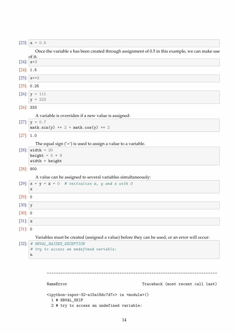
[23]: x = 0.5
Once the variable x has been created through assignment of 0.5 in this example, we can make useof it:
[24]: x*3
[24]: 1.5
[25]: x**2
[25]: 0.25
[26]: y = 111y + 222
[26]: 333
A variable is overriden if a new value is assigned:[27]: y = 0.7
math.sin(y) ** 2 + math.cos(y) ** 2
[27]: 1.0
The equal sign (’=’) is used to assign a value to a variable.[28]: width = 20
height = 5 * 9width * height
[28]: 900
A value can be assigned to several variables simultaneously:[29]: x = y = z = 0 # initialise x, y and z with 0
x
[29]: 0
[30]: y
[30]: 0
[31]: z
[31]: 0
Variables must be created (assigned a value) before they can be used, or an error will occur:[32]: # NBVAL_RAISES_EXCEPTION
# try to access an undefined variable:n
---------------------------------------------------------------------------
NameError Traceback (most recent call last)
<ipython-input-32-a15a18dc7d7c> in <module>()1 # NBVAL_SKIP2 # try to access an undefined variable:
14

----> 3 n
NameError: name 'n' is not defined
In interactive mode, the last printed expression is assigned to the variable _. This means thatwhen you are using Python as a desk calculator, it is somewhat easier to continue calculations, forexample:
[ ]: tax = 12.5 / 100price = 100.50price * tax
[ ]: price + _
This variable should be treated as read-only by the user. Don’t explicitly assign a value to it —you would create an independent local variable with the same name masking the built-in variablewith its magic behavior.
2.5.1 Terminology
Strictly speaking, the following happens when we write[ ]: x = 0.5
First, Python creates the object 0.5. Everything in Python is an object, and so is the floating pointnumber 0.5. This object is stored somewhere in memory. Next, Python binds a name to the object. Thename is x, and we often refer casually to x as a variable, an object, or even the value 0.5. However,technically, x is a name that is bound to the object 0.5. Another way to say this is that x is a referenceto the object.
While it is often sufficient to think about assigning 0.5 to a variable x, there are situations wherewe need to remember what actually happens. In particular, when we pass references to objects tofunctions, we need to realise that the function may operate on the object (rather than a copy of theobject). This is discussed in more detail in Section ??.
2.6 Impossible equations
In computer programs we often find statements like[ ]: x = x + 1
If we read this as an equation as we are use to from mathematics, x=x+1 we could subtract x onboth sides, to find that 0=1. We know this is not true, so something is wrong here.
The answer is that “equations“ in computer codes are not equations but assignments. They alwayshave to be read in the following way two-step way:
1. Evaluate the value on the right hand side of the equal sign
2. Assign this value to the variable name shown on the left hand side. (In Python: bind the nameon the left hand side to the object shown on the right hand side.)
Some computer science literature uses the following notation to express assignments and to avoidthe confusion with mathematical equations:
x ← x + 1
15

Let’s apply our two-step rule to the assignment x = x + 1 given above:
1. Evaluate the value on the right hand side of the equal sign: for this we need to know whatthe current value of x is. Let’s assume x is currently 4. In that case, the right hand side x+1evaluates to 5.
2. Assign this value (i.e. 5) to the variable name shown on the left hand side x.
Let’s confirm with the Python prompt that this is the correct interpretation:[ ]: x = 4
x = x + 1x
2.6.1 The += notation
Because it is a quite a common operation to increase a variable x by some fixed amount c, we canwrite
x += c
instead of
x = x + c
Our initial example above could thus have been written[ ]: x = 4
x += 1x
The same operators are defined for multiplication with a constant (*=), subtraction of a constant(-=) and division by a constant (/=).
Note that the order of + and = matters:[ ]: x += 1
will increase the variable x by one where as[ ]: x =+ 1
will assign the value +1 to the variable x.
3 Data Types and Data Structures
3.1 What type is it?
Python knows different data types. To find the type of a variable, use the type() function:[1]: a = 45
type(a)
[1]: int
[2]: b = 'This is a string'type(b)
[2]: str
16

[3]: c = 2 + 1jtype(c)
[3]: complex
[4]: d = [1, 3, 56]type(d)
[4]: list
3.2 Numbers
Further information
• Informal introduction to numbers. Python tutorial, section 3.1.1
• Python Library Reference: formal overview of numeric types, http://docs.python.org/library/stdtypes.html#numeric-types-int-float-long-complex
• Think Python, Sec 2.1
The in-built numerical types are integers and floating point numbers (see Section ??) and complexfloating point numbers (Section ??).
3.2.1 Integers
We have seen the use of integer numbers already in Section ??. Be aware of integer division problems(Section ??).
If we need to convert string containing an integer number to an integer we can use int() function:[5]: a = '34' # a is a string containing the characters 3 and 4
x = int(a) # x is in integer number
The function int() will also convert floating point numbers to integers:[6]: int(7.0)
[6]: 7
[7]: int(7.9)
[7]: 7
Note than int will truncate any non-integer part of a floating point number. To round an floatingpoint number to an integer, use the round() command:
[8]: round(7.9)
[8]: 8
3.2.2 Integer limits
Integers in Python 3 are unlimited; Python will automatically assign more memory as needed as thenumbers get bigger. This means we can calculate very large numbers with no special steps.
[9]: 35**42
[9]: 70934557307860443711736098025989133248003781773149967193603515625
17

In many other programming languages, such as C and FORTRAN, integers are a fixed size—mostfrequently 4 bytes, which allows 232 different values—but different types are available with differentsizes. For numbers that fit into these limits, calculations can be faster, but you may need to checkthat the numbers don’t go beyond the limits. Calculating a number beyond the limits is called integeroverflow, and may produce bizarre results.
Even in Python, we need to be aware of this when we use numpy (see Section ??). Numpy usesintegers with a fixed size, because it stores many of them together and needs to calculate with themefficiently. Numpy data types include a range of integer types named for their size, so e.g. int16 is a16-bit integer, with 216 possible values.
Integer types can also be signed or unsigned. Signed integers allow positive or negative values,unsigned integers only allow positive ones. For instance:
• uint16 (unsigned) ranges from 0 to 216 − 1• int16 (signed) ranges from −215 to 215 − 1
3.2.3 Floating Point numbers
A string containing a floating point number can be converted into a floating point number using thefloat() command:
[10]: a = '35.342'b = float(a)b
[10]: 35.342
[11]: type(b)
[11]: float
3.2.4 Complex numbers
Python (as Fortran and Matlab) has built-in complex numbers. Here are some examples how to usethese:
[12]: x = 1 + 3jx
[12]: (1+3j)
[13]: abs(x) # computes the absolute value
[13]: 3.1622776601683795
[14]: x.imag
[14]: 3.0
[15]: x.real
[15]: 1.0
[16]: x * x
[16]: (-8+6j)
[17]: x * x.conjugate()
[17]: (10+0j)
18

[18]: 3 * x
[18]: (3+9j)
Note that if you want to perform more complicated operations (such as taking the square root,etc) you have to use the cmath module (Complex MATHematics):
[19]: import cmathcmath.sqrt(x)
[19]: (1.442615274452683+1.0397782600555705j)
3.2.5 Functions applicable to all types of numbers
The abs() function returns the absolute value of a number (also called modulus):[20]: a = -45.463
abs(a)
[20]: 45.463
Note that abs() also works for complex numbers (see above).
3.3 Sequences
Strings, lists and tuples are sequences. They can be indexed and sliced in the same way.Tuples and strings are “immutable” (which basically means we can’t change individual elements
within the tuple, and we cannot change individual characters within a string) whereas lists are “mu-table” (.i.e we can change elements in a list.)
Sequences share the following operations
• a[i] returns i-th element of a• a[i:j] returns elements i up to j-1• len(a) returns number of elements in sequence• min(a) returns smallest value in sequence• max(a) returns largest value in sequence• x in a returns True if x is element in a• a + b concatenates a and b• n * a creates n copies of sequence a
3.3.1 Sequence type 1: String
Further information• Introduction to strings, Python tutorial 3.1.2
A string is a (immutable) sequence of characters. A string can be defined using single quotes:[21]: a = 'Hello World'
double quotes:[22]: a = "Hello World"
or triple quotes of either kind[23]: a = """Hello World"""
a = '''Hello World'''
The type of a string is str and the empty string is given by "":
19

[24]: a = "Hello World"type(a)
[24]: str
[25]: b = ""type(b)
[25]: str
[26]: type("Hello World")
[26]: str
[27]: type("")
[27]: str
The number of characters in a string (that is its length) can be obtained using the len()-function:[28]: a = "Hello Moon"
len(a)
[28]: 10
[29]: a = 'test'len(a)
[29]: 4
[30]: len('another test')
[30]: 12
You can combine (“concatenate”) two strings using the + operator:[31]: 'Hello ' + 'World'
[31]: 'Hello World'
Strings have a number of useful methods, including for example upper() which returns the stringin upper case:
[32]: a = "This is a test sentence."a.upper()
[32]: 'THIS IS A TEST SENTENCE.'
A list of available string methods can be found in the Python reference documentation. If a Pythonprompt is available, one should use the dir and help function to retrieve this information, i.e. dir()provides the list of methods, help can be used to learn about each method.
A particularly useful method is split() which converts a string into a list of strings:[33]: a = "This is a test sentence."
a.split()
[33]: ['This', 'is', 'a', 'test', 'sentence.']
The split() method will separate the string where it finds white space. White space means anycharacter that is printed as white space, such as one space or several spaces or a tab.
By passing a separator character to the split() method, a string can split into different parts.Suppose, for example, we would like to obtain a list of complete sentences:
20

[34]: a = "The dog is hungry. The cat is bored. The snake is awake."a.split(".")
[34]: ['The dog is hungry', ' The cat is bored', ' The snake is awake', '']
The opposite string method to split is join which can be used as follows:[35]: a = "The dog is hungry. The cat is bored. The snake is awake."
s = a.split('.')s
[35]: ['The dog is hungry', ' The cat is bored', ' The snake is awake', '']
[36]: ".".join(s)
[36]: 'The dog is hungry. The cat is bored. The snake is awake.'
[37]: " STOP".join(s)
[37]: 'The dog is hungry STOP The cat is bored STOP The snake is awake STOP'
3.3.2 Sequence type 2: List
Further information
• Introduction to Lists, Python tutorial, section 3.1.4
A list is a sequence of objects. The objects can be of any type, for example integers:[38]: a = [34, 12, 54]
or strings:[39]: a = ['dog', 'cat', 'mouse']
An empty list is presented by []:[40]: a = []
The type is list:[41]: type(a)
[41]: list
[42]: type([])
[42]: list
As with strings, the number of elements in a list can be obtained using the len() function:[43]: a = ['dog', 'cat', 'mouse']
len(a)
[43]: 3
It is also possible to mix different types in the same list:[44]: a = [123, 'duck', -42, 17, 0, 'elephant']
In Python a list is an object. It is therefor possible for a list to contain other lists (because a listkeeps a sequence of objects):
[45]: a = [1, 4, 56, [5, 3, 1], 300, 400]
You can combine (“concatenate”) two lists using the + operator:
21

[46]: [3, 4, 5] + [34, 35, 100]
[46]: [3, 4, 5, 34, 35, 100]
Or you can add one object to the end of a list using the append() method:[47]: a = [34, 56, 23]
a.append(42)a
[47]: [34, 56, 23, 42]
You can delete an object from a list by calling the remove() method and passing the object todelete. For example:
[48]: a = [34, 56, 23, 42]a.remove(56)a
[48]: [34, 23, 42]
The range() command A special type of list is frequently required (often together with for-loops)and therefor a command exists to generate that list: the range(n) command generates integers start-ing from 0 and going up to but not including n. Here are a few examples:
[49]: list(range(3))
[49]: [0, 1, 2]
[50]: list(range(10))
[50]: [0, 1, 2, 3, 4, 5, 6, 7, 8, 9]
This command is often used with for loops. For example, to print the numbers 02,12,22,32,. . . ,102,the following program can be used:
[51]: for i in range(11):print(i ** 2)
0149162536496481100
The range command takes an optional parameter for the beginning of the integer se-quence (start) and another optional parameter for the step size. This is often written asrange([start],stop,[step]) where the arguments in square brackets (i.e. start and step) are op-tional. Here are some examples:
[52]: list(range(3, 10)) # start=3
22

[52]: [3, 4, 5, 6, 7, 8, 9]
[53]: list(range(3, 10, 2)) # start=3, step=2
[53]: [3, 5, 7, 9]
[54]: list(range(10, 0, -1)) # start=10,step=-1
[54]: [10, 9, 8, 7, 6, 5, 4, 3, 2, 1]
Why are we calling list(range())?In Python 3, range() generates the numbers on demand. When you use range() in a for loop,
this is more efficient, because it doesn’t take up memory with a list of numbers. Passing it to list()forces it to generate all of its numbers, so we can see what it does.
To get the same efficient behaviour in Python 2, use xrange() instead of range().
3.3.3 Sequence type 3: Tuples
A tuple is a (immutable) sequence of objects. Tuples are very similar in behaviour to lists with theexception that they cannot be modified (i.e. are immutable).
For example, the objects in a sequence can be of any type:[55]: a = (12, 13, 'dog')
a
[55]: (12, 13, 'dog')
[56]: a[0]
[56]: 12
The parentheses are not necessary to define a tuple: just a sequence of objects separated by com-mas is sufficient to define a tuple:
[57]: a = 100, 200, 'duck'a
[57]: (100, 200, 'duck')
although it is good practice to include the paranthesis where it helps to show that tuple is defined.Tuples can also be used to make two assignments at the same time:
[58]: x, y = 10, 20x
[58]: 10
[59]: y
[59]: 20
This can be used to swap to objects within one line. For example[60]: x = 1
y = 2x, y = y, xx
[60]: 2
[61]: y
23
[61]: 1
The empty tuple is given by ()[62]: t = ()
len(t)
[62]: 0
[63]: type(t)
[63]: tuple
The notation for a tuple containing one value may seem a bit odd at first:[64]: t = (42,)
type(t)
[64]: tuple
[65]: len(t)
[65]: 1
The extra comma is required to distinguish (42,) from (42) where in the latter case the paren-thesis would be read as defining operator precedence: (42) simplifies to 42 which is just a number:
[66]: t = (42)type(t)
[66]: int
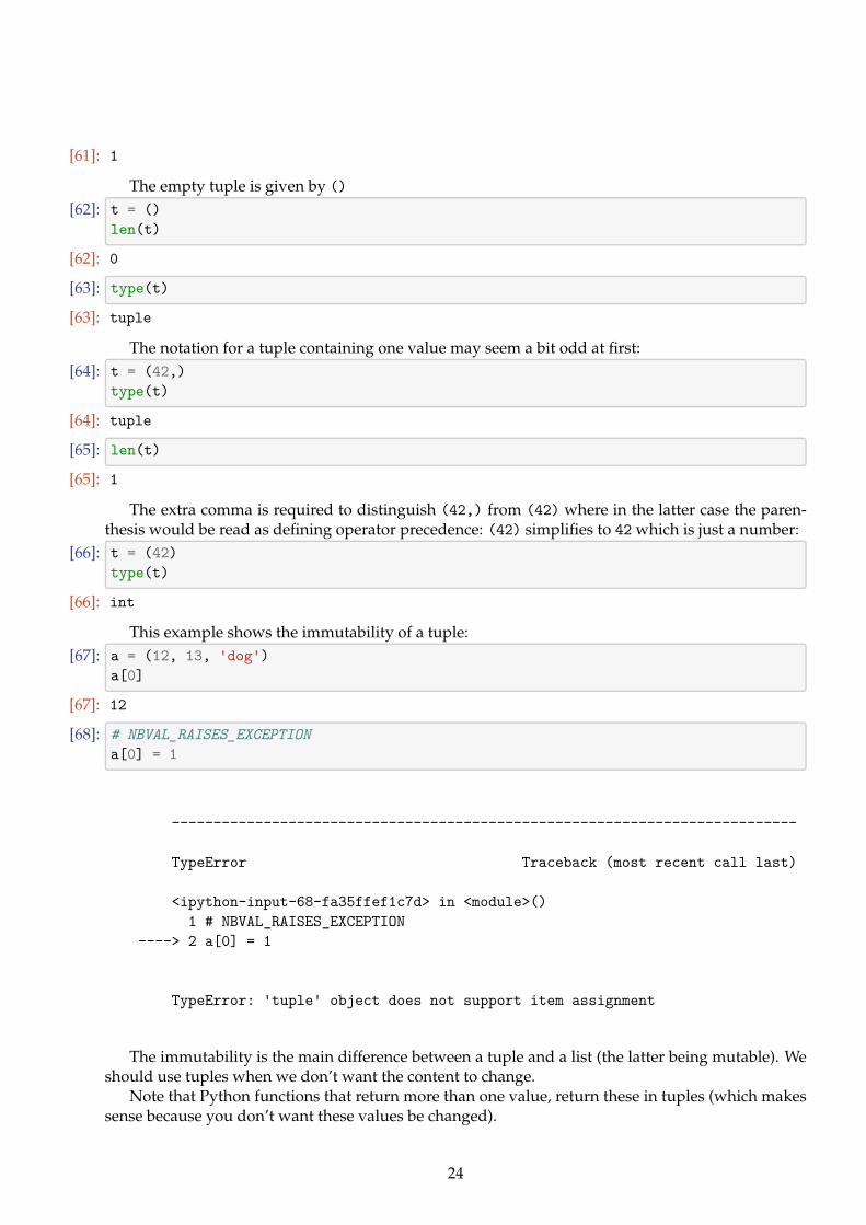
This example shows the immutability of a tuple:[67]: a = (12, 13, 'dog')
a[0]
[67]: 12
[68]: # NBVAL_RAISES_EXCEPTIONa[0] = 1
---------------------------------------------------------------------------
TypeError Traceback (most recent call last)
<ipython-input-68-fa35ffef1c7d> in <module>()1 # NBVAL_RAISES_EXCEPTION
----> 2 a[0] = 1
TypeError: 'tuple' object does not support item assignment
The immutability is the main difference between a tuple and a list (the latter being mutable). Weshould use tuples when we don’t want the content to change.
Note that Python functions that return more than one value, return these in tuples (which makessense because you don’t want these values be changed).
24

3.3.4 Indexing sequences
Further information
• Introduction to strings and indexing in Python tutorial, section 3.1.2, the relevant section isstarting after strings have been introduced.
Individual objects in lists can be accessed by using the index of the object and square brackets ([and ]):
[69]: a = ['dog', 'cat', 'mouse']a[0]
[69]: 'dog'
[70]: a[1]
[70]: 'cat'
[71]: a[2]
[71]: 'mouse'
Note that Python (like C but unlike Fortran and unlike Matlab) starts counting indices from zero!Python provides a handy shortcut to retrieve the last element in a list: for this one uses the index
“-1” where the minus indicates that it is one element from the back of the list. Similarly, the index “-2”will return the 2nd last element:
[72]: a = ['dog', 'cat', 'mouse']a[-1]
[72]: 'mouse'
[73]: a[-2]
[73]: 'cat'
If you prefer, you can think of the index a[-1] to be a shorthand notation for a[len(a) - 1].Remember that strings (like lists) are also a sequence type and can be indexed in the same way:
[74]: a = "Hello World!"a[0]
[74]: 'H'
[75]: a[1]
[75]: 'e'
[76]: a[10]
[76]: 'd'
[77]: a[-1]
[77]: '!'
[78]: a[-2]
[78]: 'd'
25

3.3.5 Slicing sequences
Further information
• Introduction to strings, indexing and slicing in Python tutorial, section 3.1.2
Slicing of sequences can be used to retrieve more than one element. For example:[79]: a = "Hello World!"
a[0:3]
[79]: 'Hel'
By writing a[0:3] we request the first 3 elements starting from element 0. Similarly:[80]: a[1:4]
[80]: 'ell'
[81]: a[0:2]
[81]: 'He'
[82]: a[0:6]
[82]: 'Hello '
We can use negative indices to refer to the end of the sequence:[83]: a[0:-1]
[83]: 'Hello World'
It is also possible to leave out the start or the end index and this will return all elements up to thebeginning or the end of the sequence. Here are some examples to make this clearer:
[84]: a = "Hello World!"a[:5]
[84]: 'Hello'
[85]: a[5:]
[85]: ' World!'
[86]: a[-2:]
[86]: 'd!'
[87]: a[:]
[87]: 'Hello World!'
Note that a[:] will generate a copy of a. The use of indices in slicing is by some people experi-enced as counter intuitive. If you feel uncomfortable with slicing, have a look at this quotation fromthe Python tutorial (section 3.1.2):
The best way to remember how slices work is to think of the indices as pointing betweencharacters, with the left edge of the first character numbered 0. Then the right edge of thelast character of a string of 5 characters has index 5, for example:
+---+---+---+---+---+| H | e | l | l | o |+---+---+---+---+---+
26

0 1 2 3 4 5 <-- use for SLICING-5 -4 -3 -2 -1 <-- use for SLICING
from the end
The first row of numbers gives the position of the slicing indices 0...5 in the string; thesecond row gives the corresponding negative indices. The slice from i to j consists of allcharacters between the edges labelled i and j, respectively.
So the important statement is that for slicing we should think of indices pointing between charac-ters.
For indexing it is better to think of the indices referring to characters. Here is a little graph sum-marising these rules:
0 1 2 3 4 <-- use for INDEXING-5 -4 -3 -2 -1 <-- use for INDEXING
+---+---+---+---+---+ from the end| H | e | l | l | o |+---+---+---+---+---+0 1 2 3 4 5 <-- use for SLICING-5 -4 -3 -2 -1 <-- use for SLICING
from the end
If you are not sure what the right index is, it is always a good technique to play around with asmall example at the Python prompt to test things before or while you write your program.
3.3.6 Dictionaries
Dictionaries are also called “associative arrays” and “hash tables”. Dictionaries are unordered sets ofkey-value pairs.
An empty dictionary can be created using curly braces:[88]: d = {}
Keyword-value pairs can be added like this:[89]: d['today'] = '22 deg C' # 'today' is the keyword
[90]: d['yesterday'] = '19 deg C'
d.keys() returns a list of all keys:[91]: d.keys()
[91]: dict_keys(['today', 'yesterday'])
We can retrieve values by using the keyword as the index:[92]: d['today']
[92]: '22 deg C'
Other ways of populating a dictionary if the data is known at creation time are:[93]: d2 = {2:4, 3:9, 4:16, 5:25}
d2
[93]: {2: 4, 3: 9, 4: 16, 5: 25}
27

[94]: d3 = dict(a=1, b=2, c=3)d3
[94]: {'a': 1, 'b': 2, 'c': 3}
The function dict() creates an empty dictionary.Other useful dictionary methods include values(), items() and get(). You can use in to check
for the presence of values.[95]: d.values()
[95]: dict_values(['22 deg C', '19 deg C'])
[96]: d.items()
[96]: dict_items([('today', '22 deg C'), ('yesterday', '19 deg C')])
[97]: d.get('today','unknown')
[97]: '22 deg C'
[98]: d.get('tomorrow','unknown')
[98]: 'unknown'
[99]: 'today' in d
[99]: True
[100]: 'tomorrow' in d
[100]: False
The method get(key,default) will provide the value for a given key if that key exists, otherwiseit will return the default object.
Here is a more complex example:[101]: # NBVAL_IGNORE_OUTPUT
order = {} # create empty dictionary
#add orders as they come inorder['Peter'] = 'Pint of bitter'order['Paul'] = 'Half pint of Hoegarden'order['Mary'] = 'Gin Tonic'
#deliver order at barfor person in order.keys():
print(person, "requests", order[person])
Peter requests Pint of bitterPaul requests Half pint of HoegardenMary requests Gin Tonic
Some more technicalities:
• The keyword can be any (immutable) Python object. This includes:
▷ numbers
▷ strings
28

▷ tuples.
• dictionaries are very fast in retrieving values (when given the key)
An other example to demonstrate an advantage of using dictionaries over pairs of lists:[102]: # NBVAL_IGNORE_OUTPUT
dic = {} #create empty dictionary
dic["Hans"] = "room 1033" #fill dictionarydic["Andy C"] = "room 1031" #"Andy C" is keydic["Ken"] = "room 1027" #"room 1027" is value
for key in dic.keys():print(key, "works in", dic[key])
Hans works in room 1033Andy C works in room 1031Ken works in room 1027
Without dictionary:[103]: people = ["Hans","Andy C","Ken"]
rooms = ["room 1033","room 1031","room 1027"]
#possible inconsistency here since we have two listsif not len( people ) == len( rooms ):
raise RuntimeError("people and rooms differ in length")
for i in range( len( rooms ) ):print(people[i],"works in",rooms[i])
Hans works in room 1033Andy C works in room 1031Ken works in room 1027
3.4 Passing arguments to functions
This section contains some more advanced ideas and makes use of concepts that are only later intro-duced in this text. The section may be more easily accessible at a later stage.
When objects are passed to a function, Python always passes (the value of) the reference to theobject to the function. Effectively this is calling a function by reference, although one could refer to itas calling by value (of the reference).
We review argument passing by value and reference before discussing the situation in Python inmore detail.
3.4.1 Call by value
One might expect that if we pass an object by value to a function, that modifications of that valueinside the function will not affect the object (because we don’t pass the object itself, but only its value,which is a copy). Here is an example of this behaviour (in C):
29

#include <stdio.h>
void pass_by_value(int m) {printf("in pass_by_value: received m=%d\n",m);m=42;printf("in pass_by_value: changed to m=%d\n",m);
}
int main(void) {int global_m = 1;printf("global_m=%d\n",global_m);pass_by_value(global_m);printf("global_m=%d\n",global_m);return 0;
}
together with the corresponding output:
global_m=1in pass_by_value: received m=1in pass_by_value: changed to m=42global_m=1
The value 1 of the global variable global_m is not modified when the function pass_by_valuechanges its input argument to 42.
3.4.2 Call by reference
Calling a function by reference, on the other hand, means that the object given to a function is areference to the object. This means that the function will see the same object as in the calling code(because they are referencing the same object: we can think of the reference as a pointer to the placein memory where the object is located). Any changes acting on the object inside the function, willthen be visible in the object at the calling level (because the function does actually operate on thesame object, not a copy of it).
Here is one example showing this using pointers in C:
#include <stdio.h>
void pass_by_reference(int *m) {printf("in pass_by_reference: received m=%d\n",*m);*m=42;printf("in pass_by_reference: changed to m=%d\n",*m);
}
int main(void) {int global_m = 1;printf("global_m=%d\n",global_m);pass_by_reference(&global_m);printf("global_m=%d\n",global_m);return 0;
}
30

together with the corresponding output:
global_m=1in pass_by_reference: received m=1in pass_by_reference: changed to m=42global_m=42
C++ provides the ability to pass arguments as references by adding an ampersand in front of theargument name in the function definition:
#include <stdio.h>
void pass_by_reference(int &m) {printf("in pass_by_reference: received m=%d\n",m);m=42;printf("in pass_by_reference: changed to m=%d\n",m);
}
int main(void) {int global_m = 1;printf("global_m=%d\n",global_m);pass_by_reference(global_m);printf("global_m=%d\n",global_m);return 0;
}
together with the corresponding output:
global_m=1in pass_by_reference: received m=1in pass_by_reference: changed to m=42global_m=42
3.4.3 Argument passing in Python
In Python, objects are passed as the value of a reference (think pointer) to the object. Depending onthe way the reference is used in the function and depending on the type of object it references, thiscan result in pass-by-reference behaviour (where any changes to the object received as a functionargument, are immediately reflected in the calling level).
Here are three examples to discuss this. We start by passing a list to a function which iteratesthrough all elements in the sequence and doubles the value of each element:
[104]: def double_the_values(l):print("in double_the_values: l = %s" % l)for i in range(len(l)):
l[i] = l[i] * 2print("in double_the_values: changed l to l = %s" % l)
l_global = [0, 1, 2, 3, 10]print("In main: s=%s" % l_global)double_the_values(l_global)print("In main: s=%s" % l_global)
31

In main: s=[0, 1, 2, 3, 10]in double_the_values: l = [0, 1, 2, 3, 10]in double_the_values: changed l to l = [0, 2, 4, 6, 20]In main: s=[0, 2, 4, 6, 20]
The variable l is a reference to the list object. The line l[i] = l[i] * 2 first evaluates the right-hand side and reads the element with index i, then multiplies this by two. A reference to this newobject is then stored in the list object l at position with index i. We have thus modified the list object,that is referenced through l.
The reference to the list object does never change: the line l[i] = l[i] * 2 changes the elementsl[i] of the list l but never changes the reference l for the list. Thus both the function and callinglevel are operating on the same object through the references l and global_l, respectively.
In contrast, here is an example where do not modify the elements of the list within the function:which produces this output:
[105]: def double_the_list(l):print("in double_the_list: l = %s" % l)l = l + lprint("in double_the_list: changed l to l = %s" % l)
l_global = "Hello"print("In main: l=%s" % l_global)double_the_list(l_global)print("In main: l=%s" % l_global)
In main: l=Helloin double_the_list: l = Helloin double_the_list: changed l to l = HelloHelloIn main: l=Hello
What happens here is that during the evaluation of l = l + l a new object is created that holdsl + l, and that we then bind the name l to it. In the process, we lose the references to the list objectl that was given to the function (and thus we do not change the list object given to the function).
Finally, let’s look at which produces this output:[106]: def double_the_value(l):
print("in double_the_value: l = %s" % l)l = 2 * lprint("in double_the_values: changed l to l = %s" % l)
l_global = 42print("In main: s=%s" % l_global)double_the_value(l_global)print("In main: s=%s" % l_global)
In main: s=42in double_the_value: l = 42in double_the_values: changed l to l = 84In main: s=42
In this example, we also double the value (from 42 to 84) within the function. However, whenwe bind the object 84 to the python name l (that is the line l = l * 2) we have created a new object
32

(84), and we bind the new object to l. In the process, we lose the reference to the object 42 within thefunction. This does not affect the object 42 itself, nor the reference l_global to it.
In summary, Python’s behaviour of passing arguments to a function may appear to vary (if weview it from the pass by value versus pass by reference point of view). However, it is always call byvalue, where the value is a reference to the object in question, and the behaviour can be explainedthrough the same reasoning in every case.
3.4.4 Performance considerations
Call by value function calls require copying of the value before it is passed to the function. From aperformance point of view (both execution time and memory requirements), this can be an expensiveprocess if the value is large. (Imagine the value is a numpy.array object which could be severalMegabytes or Gigabytes in size.)
One generally prefers call by reference for large data objects as in this case only a pointer to thedata objects is passed, independent of the actual size of the object, and thus this is generally fasterthan call-by-value.
Python’s approach of (effectively) calling by reference is thus efficient. However, we need to becareful that our function do not modify the data they have been given where this is undesired.
3.4.5 Inadvertent modification of data
Generally, a function should not modify the data given as input to it.For example, the following code demonstrates the attempt to determine the maximum value of a
list, and – inadvertently – modifies the list in the process:[107]: def mymax(s): # demonstrating side effect
if len(s) == 0:raise ValueError('mymax() arg is an empty sequence')
elif len(s) == 1:return s[0]
else:for i in range(1, len(s)):
if s[i] < s[i - 1]:s[i] = s[i - 1]
return s[len(s) - 1]
s = [-45, 3, 6, 2, -1]print("in main before caling mymax(s): s=%s" % s)print("mymax(s)=%s" % mymax(s))print("in main after calling mymax(s): s=%s" % s)
in main before caling mymax(s): s=[-45, 3, 6, 2, -1]mymax(s)=6in main after calling mymax(s): s=[-45, 3, 6, 6, 6]
The user of the mymax() function would not expect that the input argument is modified when thefunction executes. We should generally avoid this. There are several ways to find better solutions tothe given problem:
• In this particular case, we could use the Python in-built function max() to obtain the maximumvalue of a sequence.
33

• If we felt we need to stick to storing temporary values inside the list [this is actually not neces-sary], we could create a copy of the incoming list s first, and then proceed with the algorithm(see Section ?? on Copying objects).
• Use another algorithm which uses an extra temporary variable rather than abusing the list forthis. For example:
• We could pass a tuple (instead of a list) to the function: a tuple is immutable and can thus neverbe modified (this would result in an exception being raised when the function tries to write toelements in the tuple).
3.4.6 Copying objects
Python provides the id() function which returns an integer number that is unique for each object.(In the current CPython implementation, this is the memory address.) We can use this to identifywhether two objects are the same.
To copy a sequence object (including lists), we can slice it, i.e. if a is a list, then a[:] will return acopy of a. Here is a demonstration:
[108]: a = list(range(10))a
[108]: [0, 1, 2, 3, 4, 5, 6, 7, 8, 9]
[109]: b = ab[0] = 42a # changing b changes a
[109]: [42, 1, 2, 3, 4, 5, 6, 7, 8, 9]
[110]: # NBVAL_IGNORE_OUTPUTid(a)
[110]: 4446565320
[111]: # NBVAL_IGNORE_OUTPUTid(b)
[111]: 4446565320
[112]: # NBVAL_IGNORE_OUTPUTc = a[:]id(c) # c is a different object
[112]: 4444418824
[113]: c[0] = 100a # changing c does not affect a
[113]: [42, 1, 2, 3, 4, 5, 6, 7, 8, 9]
Python’s standard library provides the copy module, which provides copy functions that can beused to create copies of objects. We could have used import copy; c = copy.deepcopy(a) insteadof c = a[:].
3.5 Equality and Identity/Sameness
A related question concerns the equality of objects.
34

3.5.1 Equality
The operators <, >, ==, >=, <=, and != compare the values of two objects. The objects need not have thesame type. For example:
[114]: a = 1.0; b = 1type(a)
[114]: float
[115]: type(b)
[115]: int
[116]: a == b
[116]: True
So the == operator checks whether the values of two objects are equal.
3.5.2 Identity / Sameness
To see check whether two objects a and b are the same (i.e. a and b are references to the same placein memory), we can use the is operator (continued from example above):
[117]: a is b
[117]: False
Of course they are different here, as they are not of the same type.We can also ask the id function which, according to the documentation string in Python 2.7 “Re-
turns the identity of an object. This is guaranteed to be unique among simultaneously existing objects. (Hint:it’s the object’s memory address.)”
[118]: # NBVAL_IGNORE_OUTPUTid(a)
[118]: 4446045984
[119]: # NBVAL_IGNORE_OUTPUTid(b)
[119]: 4406101840
which shows that a and b are stored in different places in memory.
3.5.3 Example: Equality and identity
We close with an example involving lists:[120]: x = [0, 1, 2]
y = xx == y
[120]: True
[121]: x is y
[121]: True
[122]: # NBVAL_IGNORE_OUTPUTid(x)
35

[122]: 4445528520
[123]: # NBVAL_IGNORE_OUTPUTid(y)
[123]: 4445528520
Here, x and y are references to the same piece of memory, they are thus identical and the isoperator confirms this. The important point to remember is that line 2 (y=x) creates a new referencey to the same list object that x is a reference for.
Accordingly, we can change elements of x, and y will change simultaneously as both x and y referto the same object:
[124]: x
[124]: [0, 1, 2]
[125]: y
[125]: [0, 1, 2]
[126]: x is y
[126]: True
[127]: x[0] = 100y
[127]: [100, 1, 2]
[128]: x
[128]: [100, 1, 2]
In contrast, if we use z=x[:] (instead of z=x) to create a new name z, then the slicing operationx[:] will actually create a copy of the list x, and the new reference z will point to the copy. The valueof x and z is equal, but x and z are not the same object (they are not identical):
[129]: x
[129]: [100, 1, 2]
[130]: z = x[:] # create copy of x before assigning to zz == x # same value
[130]: True
[131]: z is x # are not the same object
[131]: False
[132]: # NBVAL_IGNORE_OUTPUTid(z) # confirm by looking at ids
[132]: 4446678088
[133]: # NBVAL_IGNORE_OUTPUTid(x)
[133]: 4445528520
[134]: x
36

[134]: [100, 1, 2]
[135]: z
[135]: [100, 1, 2]
Consequently, we can change x without changing z, for example (continued)[136]: x[0] = 42
x
[136]: [42, 1, 2]
[137]: z
[137]: [100, 1, 2]
4 Introspection
A Python code can ask and answer questions about itself and the objects it is manipulating.
4.1 dir()
dir() is a built-in function which returns a list of all the names belonging to some namespace.
• If no arguments are passed to dir (i.e. dir()), it inspects the namespace in which it was called.
• If dir is given an argument (i.e. dir(<object>), then it inspects the namespace of the objectwhich it was passed.
For example:[1]: # NBVAL_IGNORE_OUTPUT
apples = ['Cox', 'Braeburn', 'Jazz']dir(apples)
[1]: ['__add__','__class__','__contains__','__delattr__','__delitem__','__dir__','__doc__','__eq__','__format__','__ge__','__getattribute__','__getitem__','__gt__','__hash__','__iadd__','__imul__','__init__','__init_subclass__','__iter__',
37

'__le__','__len__','__lt__','__mul__','__ne__','__new__','__reduce__','__reduce_ex__','__repr__','__reversed__','__rmul__','__setattr__','__setitem__','__sizeof__','__str__','__subclasshook__','append','clear','copy','count','extend','index','insert','pop','remove','reverse','sort']
[1]: # NBVAL_IGNORE_OUTPUTdir()
[1]: ['In','Out','_','__','___','__builtin__','__builtins__','__doc__','__loader__','__name__','__package__','__spec__','_dh','_i','_i1','_ih','_ii','_iii','_oh',
38
'_sh','exit','get_ipython','quit']
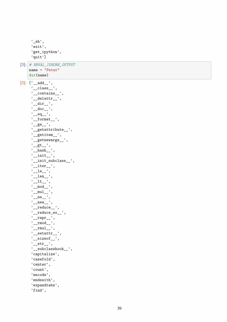
[3]: # NBVAL_IGNORE_OUTPUTname = "Peter"dir(name)
[3]: ['__add__','__class__','__contains__','__delattr__','__dir__','__doc__','__eq__','__format__','__ge__','__getattribute__','__getitem__','__getnewargs__','__gt__','__hash__','__init__','__init_subclass__','__iter__','__le__','__len__','__lt__','__mod__','__mul__','__ne__','__new__','__reduce__','__reduce_ex__','__repr__','__rmod__','__rmul__','__setattr__','__sizeof__','__str__','__subclasshook__','capitalize','casefold','center','count','encode','endswith','expandtabs','find',
39

'format','format_map','index','isalnum','isalpha','isdecimal','isdigit','isidentifier','islower','isnumeric','isprintable','isspace','istitle','isupper','join','ljust','lower','lstrip','maketrans','partition','replace','rfind','rindex','rjust','rpartition','rsplit','rstrip','split','splitlines','startswith','strip','swapcase','title','translate','upper','zfill']
4.1.1 Magic names
You will find many names which both start and end with a double underscore (e.g. __name__).These are called magic names. Functions with magic names provide the implementation of particularpython functionality.
For example, the application of the str to an object a, i.e. str(a), will – internally – result in themethod a.__str__() being called. This method __str__ generally needs to return a string. The ideais that the __str__() method should be defined for all objects (including those that derive from newclasses that a programmer may create) so that all objects (independent of their type or class) can beprinted using the str() function. The actual conversion of some object x to the string is then donevia the object specific method x.__str__().
We can demonstrate this by creating a class my_int which inherits from the Python’s integer baseclass, and overrides the __str__ method. (It requires more Python knowledge than provided up to
40

this point in the text to be able to understand this example.)[4]: class my_int(int):
"""Inherited from int"""def __str__(self):
"""Tailored str representation of my int"""return "my_int: %s" % (int.__str__(self))
a = my_int(3)b = int(4) # equivalent to b = 4print("a * b = ", a * b)print("Type a = ", type(a), "str(a) = ", str(a))print("Type b = ", type(b), "str(b) = ", str(b))
a * b = 12Type a = <class '__main__.my_int'> str(a) = my_int: 3Type b = <class 'int'> str(b) = 4
Further Reading See Python documentation, Data Model
4.2 type
The type(<object>) command returns the type of an object:[5]: type(1)
[5]: int
[6]: type(1.0)
[6]: float
[7]: type("Python")
[7]: str
[8]: import mathtype(math)
[8]: module
[9]: type(math.sin)
[9]: builtin_function_or_method
4.3 isinstance
isinstance(<object>, <typespec>) returns True if the given object is an instance of the given type,or any of its superclasses. Use help(isinstance) for the full syntax.
[10]: isinstance(2,int)
[10]: True
[11]: isinstance(2.,int)
[11]: False
41

[12]: isinstance(a,int) # a is an instance of my_int
[12]: True
[13]: type(a)
[13]: __main__.my_int
4.4 help
• The help(<object>) function will report the docstring (magic attritube with name __doc__) ofthe object that it is given, sometimes complemented with additional information. In the caseof functions, help will also show the list of arguments that the function accepts (but it cannotprovide the return value).
• help() starts an interactive help environment.
• It is common to use the help command a lot to remind oneself of the syntax and semantic ofcommands.
[14]: help(isinstance)
Help on built-in function isinstance in module builtins:
isinstance(obj, class_or_tuple, /)Return whether an object is an instance of a class or of a subclass thereof.
A tuple, as in ``isinstance(x, (A, B, ...))``, may be given as the target tocheck against. This is equivalent to ``isinstance(x, A) or isinstance(x, B)or ...`` etc.
[15]: # NBVAL_IGNORE_OUTPUTimport mathhelp(math.sin)
Help on built-in function sin in module math:
sin(...)sin(x)
Return the sine of x (measured in radians).
[16]: # NBVAL_IGNORE_OUTPUThelp(math)
Help on module math:
NAMEmath
42

MODULE REFERENCEhttps://docs.python.org/3.6/library/math
The following documentation is automatically generated from the Pythonsource files. It may be incomplete, incorrect or include features thatare considered implementation detail and may vary between Pythonimplementations. When in doubt, consult the module reference at thelocation listed above.
DESCRIPTIONThis module is always available. It provides access to themathematical functions defined by the C standard.
FUNCTIONSacos(...)
acos(x)
Return the arc cosine (measured in radians) of x.
acosh(...)acosh(x)
Return the inverse hyperbolic cosine of x.
asin(...)asin(x)
Return the arc sine (measured in radians) of x.
asinh(...)asinh(x)
Return the inverse hyperbolic sine of x.
atan(...)atan(x)
Return the arc tangent (measured in radians) of x.
atan2(...)atan2(y, x)
Return the arc tangent (measured in radians) of y/x.Unlike atan(y/x), the signs of both x and y are considered.
atanh(...)atanh(x)
Return the inverse hyperbolic tangent of x.
43

ceil(...)ceil(x)
Return the ceiling of x as an Integral.This is the smallest integer >= x.
copysign(...)copysign(x, y)
Return a float with the magnitude (absolute value) of x but the signof y. On platforms that support signed zeros, copysign(1.0, -0.0)returns -1.0.
cos(...)cos(x)
Return the cosine of x (measured in radians).
cosh(...)cosh(x)
Return the hyperbolic cosine of x.
degrees(...)degrees(x)
Convert angle x from radians to degrees.
erf(...)erf(x)
Error function at x.
erfc(...)erfc(x)
Complementary error function at x.
exp(...)exp(x)
Return e raised to the power of x.
expm1(...)expm1(x)
Return exp(x)-1.This function avoids the loss of precision involved in the direct
evaluation of exp(x)-1 for small x.
44

fabs(...)fabs(x)
Return the absolute value of the float x.
factorial(...)factorial(x) -> Integral
Find x!. Raise a ValueError if x is negative or non-integral.
floor(...)floor(x)
Return the floor of x as an Integral.This is the largest integer <= x.
fmod(...)fmod(x, y)
Return fmod(x, y), according to platform C. x % y may differ.
frexp(...)frexp(x)
Return the mantissa and exponent of x, as pair (m, e).m is a float and e is an int, such that x = m * 2.**e.If x is 0, m and e are both 0. Else 0.5 <= abs(m) < 1.0.
fsum(...)fsum(iterable)
Return an accurate floating point sum of values in the iterable.Assumes IEEE-754 floating point arithmetic.
gamma(...)gamma(x)
Gamma function at x.
gcd(...)gcd(x, y) -> intgreatest common divisor of x and y
hypot(...)hypot(x, y)
Return the Euclidean distance, sqrt(x*x + y*y).
isclose(...)
45

isclose(a, b, *, rel_tol=1e-09, abs_tol=0.0) -> bool
Determine whether two floating point numbers are close in value.
rel_tolmaximum difference for being considered "close", relative to themagnitude of the input values
abs_tolmaximum difference for being considered "close", regardless of
themagnitude of the input values
Return True if a is close in value to b, and False otherwise.
For the values to be considered close, the difference between themmust be smaller than at least one of the tolerances.
-inf, inf and NaN behave similarly to the IEEE 754 Standard. Thatis, NaN is not close to anything, even itself. inf and -inf areonly close to themselves.
isfinite(...)isfinite(x) -> bool
Return True if x is neither an infinity nor a NaN, and False otherwise.
isinf(...)isinf(x) -> bool
Return True if x is a positive or negative infinity, and Falseotherwise.
isnan(...)isnan(x) -> bool
Return True if x is a NaN (not a number), and False otherwise.
ldexp(...)ldexp(x, i)
Return x * (2**i).
lgamma(...)lgamma(x)
Natural logarithm of absolute value of Gamma function at x.
log(...)log(x[, base])
46

Return the logarithm of x to the given base.If the base not specified, returns the natural logarithm (base e) of x.
log10(...)log10(x)
Return the base 10 logarithm of x.
log1p(...)log1p(x)
Return the natural logarithm of 1+x (base e).The result is computed in a way which is accurate for x near zero.
log2(...)log2(x)
Return the base 2 logarithm of x.
modf(...)modf(x)
Return the fractional and integer parts of x. Both results carry thesign
of x and are floats.
pow(...)pow(x, y)
Return x**y (x to the power of y).
radians(...)radians(x)
Convert angle x from degrees to radians.
sin(...)sin(x)
Return the sine of x (measured in radians).
sinh(...)sinh(x)
Return the hyperbolic sine of x.
sqrt(...)sqrt(x)
Return the square root of x.
47

tan(...)tan(x)
Return the tangent of x (measured in radians).
tanh(...)tanh(x)
Return the hyperbolic tangent of x.
trunc(...)trunc(x:Real) -> Integral
Truncates x to the nearest Integral toward 0. Uses the __trunc__ magicmethod.
DATAe = 2.718281828459045inf = infnan = nanpi = 3.141592653589793tau = 6.283185307179586
FILE/Users/fangohr/anaconda3/lib/python3.6/lib-
dynload/math.cpython-36m-darwin.so
The help function needs to be given the name of an object (which must exist in the current namespace). For example pyhelp(math.sqrt) will not work if the math module has not been importedbefore
[17]: # NBVAL_IGNORE_OUTPUThelp(math.sqrt)
Help on built-in function sqrt in module math:
sqrt(...)sqrt(x)
Return the square root of x.
[18]: # NBVAL_IGNORE_OUTPUTimport mathhelp(math.sqrt)
Help on built-in function sqrt in module math:
48

sqrt(...)sqrt(x)
Return the square root of x.
Instead of importing the module, we could also have given the string of math.sqrt to the helpfunction, i.e.:
[19]: # NBVAL_IGNORE_OUTPUThelp('math.sqrt')
Help on built-in function sqrt in math:
math.sqrt = sqrt(...)sqrt(x)
Return the square root of x.
help is a function which gives information about the object which is passed as its argument. Mostthings in Python (classes, functions, modules, etc.) are objects, and therefor can be passed to help.There are, however, some things on which you might like to ask for help, which are not existingPython objects. In such cases it is often possible to pass a string containing the name of the thing orconcept to help, for example
• help(modules) will generate a list of all modules which can be imported into the current in-terpreter. Note that help(modules) (note absence of quotes) will result in a NameError (unlessyou are unlucky enough to have a variable called modules floating around, in which case youwill get help on whatever that variable happens to refer to.)
• help(some_module), where some_module is a module which has not been imported yet (andtherefor isn’t an object yet), will give you that module’s help information.
• help(some_keyword): For example and, if or print (i.e. help(and), help(if) andhelp(print)). These are special words recognized by Python: they are not objects and thuscannot be passed as arguments to help. Passing the name of the keyword as a string to helpworks, but only if you have Python’s HTML documentation installed, and the interpreter hasbeen made aware of its location by setting the environment variable PYTHONDOCS.
4.5 Docstrings
The command help(<object>) accesses the documentation strings of objects.Any literal string apparing as the first item in the definition of a class, function, method or mod-
ule, is taken to be its docstring.help includes the docstring in the information it displays about the object.In addition to the docstring it may display some other information, for example, in the case of
functions, it displays the function’s signature.The docstring is stored in the object’s __doc__ attribute.
[20]: # NBVAL_IGNORE_OUTPUThelp(math.sin)
49

Help on built-in function sin in module math:
sin(...)sin(x)
Return the sine of x (measured in radians).
[21]: # NBVAL_IGNORE_OUTPUTprint(math.sin.__doc__)
sin(x)
Return the sine of x (measured in radians).
For user-defined functions, classes, types, modules, . . . ), one should always provide a docstring.Documenting a user-provided function:
[22]: def power2and3(x):"""Returns the tuple (x**2, x**3)"""return x**2 ,x**3
power2and3(2)
[22]: (4, 8)
[23]: power2and3(4.5)
[23]: (20.25, 91.125)
[24]: power2and3(0+1j)
[24]: ((-1+0j), (-0-1j))
[25]: help(power2and3)
Help on function power2and3 in module __main__:
power2and3(x)Returns the tuple (x**2, x**3)
[26]: print(power2and3.__doc__)
Returns the tuple (x**2, x**3)
5 Input and Output
In this section, we describe printing, which includes the use of the print function, the old-style %format specifiers and the new style {} format specifiers.
50

5.1 Printing to standard output (normally the screen)
The print function is the most commonly used command to print information to the “standardoutput device” which is normally the screen.
There are two modes to use print.
5.1.1 Simple print
The easiest way to use the print command is to list the variables to be printed, separated by comma.Here are a few examples:
[1]: a = 10b = 'test text'print(a)
10
[2]: print(b)
test text
[3]: print(a, b)
10 test text
[4]: print("The answer is", a)
The answer is 10
[5]: print("The answer is", a, "and the string contains", b)
The answer is 10 and the string contains test text
[6]: print("The answer is", a, "and the string reads", b)
The answer is 10 and the string reads test text
Python adds a space between every object that is being printed.Python prints a new line after every print call. To suppress that, use the end= parameter:
[7]: print("Printing in line one", end='')print("...still printing in line one.")
Printing in line one...still printing in line one.
5.1.2 Formatted printing
The more sophisticated way of formatting output uses a syntax very similar to Matlab’s fprintf(and therefor also similar to C’s printf).
The overall structure is that there is a string containing format specifiers, followed by a percentagesign and a tuple that contains the variables to be printed in place of the format specifiers.
51

[8]: print("a = %d b = %d" % (10,20))
a = 10 b = 20
A string can contain format identifiers (such as %f to format as a float, %d to format as an integer,and %s to format as a string):
[9]: from math import piprint("Pi = %5.2f" % pi)
Pi = 3.14
[10]: print("Pi = %10.3f" % pi)
Pi = 3.142
[11]: print("Pi = %10.8f" % pi)
Pi = 3.14159265
[12]: print("Pi = %d" % pi)
Pi = 3
The format specifier of type %W.Df means that a Float should be printed with a total Width of Wcharacters and D digits behind the Decimal point. (This is identical to Matlab and C, for example.)
To print more than one object, provide multiple format specifiers and list several objects in thetuple:
[13]: print("Pi = %f, 142*pi = %f and pi^2 = %f." % (pi,142*pi,pi**2))
Pi = 3.141593, 142*pi = 446.106157 and piˆ2 = 9.869604.
Note that the conversion of a format specifier and a tuple of variables into string does not rely onthe print command:
[14]: from math import pi"pi = %f" % pi
[14]: 'pi = 3.141593'
This means that we can convert objects into strings whereever we need, and we can decide toprint the strings later – there is no need to couple the formatting closely to the code that does theprinting.
Overview of commonly used format specifiers using the astronomical unit as an example:[15]: AU = 149597870700 # astronomical unit [m]
"%f" % AU # line 1 in table
[15]: '149597870700.000000'
52

specifier style Example output for AU
%f floating point 149597870700.000000%e exponential notation 1.495979e+11%g shorter of %e or %f 1.49598e+11%d integer 149597870700%s str() 149597870700%r repr() 149597870700L
5.1.3 “str” and “__str__”
All objects in Python should provide a method __str__ which returns a nice string representation ofthe object. This method a.__str__() is called when we apply the str function to object a:
[16]: a = 3.14a.__str__()
[16]: '3.14'
[17]: str(a)
[17]: '3.14'
The str function is extremely convenient as it allows us to print more complicated objects, suchas
[18]: b = [3, 4.2, ['apple', 'banana'], (0, 1)]str(b)
[18]: "[3, 4.2, ['apple', 'banana'], (0, 1)]"
The way Python prints this is that it uses the __str__ method of the list object. This will print theopening square bracket [ and then call the __str__ method of the first object, i.e. the integer 3. Thiswill produce 3. Then the list object’s __str__ method prints the comma , and moves on to call the__str__ method of the next element in the list (i.e. 4.2) to print itself. This way any composite objectcan be represented as a string by asking the objects it holds to convert themselves to strings.
The string method of object x is called implicitly, when we
• use the “%s” format specifier to print x
• pass the object x directly to the print command:
[19]: print(b)
[3, 4.2, ['apple', 'banana'], (0, 1)]
[20]: print("%s" % b)
[3, 4.2, ['apple', 'banana'], (0, 1)]
5.1.4 “repr” and “__repr__”
A second function, repr, should convert a given object into a string presentation so that this string canbe used to re-created the object using the eval function. The repr function will generally provide a moredetailed string than str. Applying repr to the object x will attempt to call x.__repr__().
53

[21]: from math import pi as a1str(a1)
[21]: '3.141592653589793'
[22]: repr(a1)
[22]: '3.141592653589793'
[23]: number_as_string = repr(a1)a2 = eval(number_as_string) # evaluate stringa2
[23]: 3.141592653589793
[24]: a2-a1 # -> repr is exact representation
[24]: 0.0
[25]: a1-eval(repr(a1))
[25]: 0.0
[26]: a1-eval(str(a1)) # -> str has lost a few digits
[26]: 0.0
We can convert an object to its str() or repr presentation using the format specifiers %s and%r,respectively.
[27]: import math"%s" % math.pi
[27]: '3.141592653589793'
[28]: "%r" % math.pi
[28]: '3.141592653589793'
5.1.5 New-style string formatting
A new system of built-in formatting allows more flexibility for complex cases, at the cost of being abit longer.
Basic ideas in examples:[29]: "{} needs {} pints".format('Peter', 4) # insert values in order
[29]: 'Peter needs 4 pints'
[30]: "{0} needs {1} pints".format('Peter', 4) # index which element
[30]: 'Peter needs 4 pints'
[31]: "{1} needs {0} pints".format('Peter', 4)
[31]: '4 needs Peter pints'
[32]: "{name} needs {number} pints".format( # reference element toname='Peter',number=4) # print by name
[32]: 'Peter needs 4 pints'
54
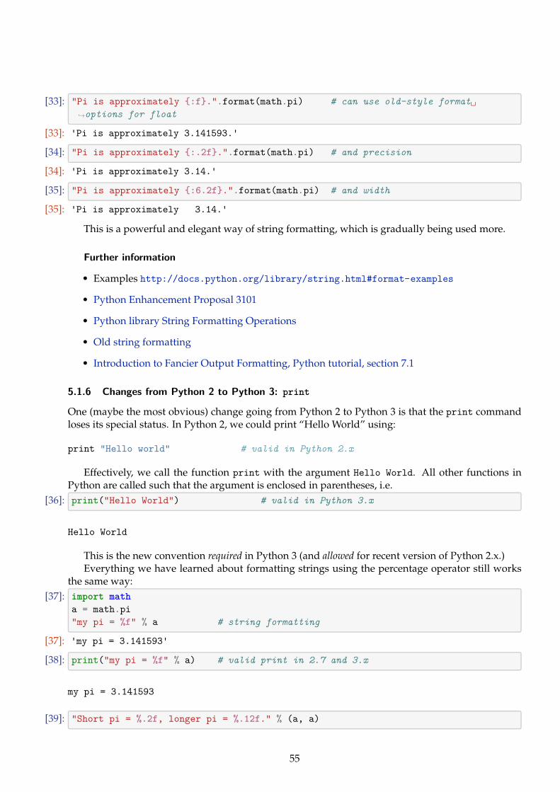
[33]: "Pi is approximately {:f}.".format(math.pi) # can use old-style format␣↪→options for float
[33]: 'Pi is approximately 3.141593.'
[34]: "Pi is approximately {:.2f}.".format(math.pi) # and precision
[34]: 'Pi is approximately 3.14.'
[35]: "Pi is approximately {:6.2f}.".format(math.pi) # and width
[35]: 'Pi is approximately 3.14.'
This is a powerful and elegant way of string formatting, which is gradually being used more.
Further information
• Examples http://docs.python.org/library/string.html#format-examples
• Python Enhancement Proposal 3101
• Python library String Formatting Operations
• Old string formatting
• Introduction to Fancier Output Formatting, Python tutorial, section 7.1
5.1.6 Changes from Python 2 to Python 3: print
One (maybe the most obvious) change going from Python 2 to Python 3 is that the print commandloses its special status. In Python 2, we could print “Hello World” using:
print "Hello world" # valid in Python 2.x
Effectively, we call the function print with the argument Hello World. All other functions inPython are called such that the argument is enclosed in parentheses, i.e.
[36]: print("Hello World") # valid in Python 3.x
Hello World
This is the new convention required in Python 3 (and allowed for recent version of Python 2.x.)Everything we have learned about formatting strings using the percentage operator still works
the same way:[37]: import math
a = math.pi"my pi = %f" % a # string formatting
[37]: 'my pi = 3.141593'
[38]: print("my pi = %f" % a) # valid print in 2.7 and 3.x
my pi = 3.141593
[39]: "Short pi = %.2f, longer pi = %.12f." % (a, a)
55

[39]: 'Short pi = 3.14, longer pi = 3.141592653590.'
[40]: print("Short pi = %.2f, longer pi = %.12f." % (a, a))
Short pi = 3.14, longer pi = 3.141592653590.
[41]: print("Short pi = %.2f, longer pi = %.12f." % (a, a))
Short pi = 3.14, longer pi = 3.141592653590.
[42]: # 1. Write a fileout_file = open("test.txt", "w") #'w' stands for Writingout_file.write("Writing text to file. This is the first line.\n"+\
"And the second line.")out_file.close() #close the file
# 2. Read a filein_file = open("test.txt", "r") #'r' stands for Readingtext = in_file.read() #read complete file into
#string variable textin_file.close() #close the file
# 3. Display dataprint(text)
Writing text to file. This is the first line.And the second line.
5.2 Reading and writing files
Here is a program that
1. writes some text to a file with name test.txt,
2. and then reads the text again and
3. prints it to the screen.
The data stored in the file test.txt is:
Writing text to file. This is the first line.And the second line.
In more detail, you have opened a file with the open command, and assigned this open file objectto the variable out_file. We have then written data to the file using the out_file.write method.Note that in the example above, we have given a string to the write method. We can, of course,use all the formatting that we have discussed before—see Section ?? and Section ??. For example,to write this file with name table table.txt we can use this Python program It is good practice toclose() files when we have finished reading and writing. If a Python program is left in a controlledway (i.e. not through a power cut or an unlikely bug deep in the Python language or the operatingsystem) then it will close all open files as soon as the file objects are destroyed. However, closingthem actively as soon as possible is better style.
56

5.2.1 File reading examples
We use a file named myfile.txt containing the following 3 lines of text for the examples below:
This is the first line.This is the second line.This is a third and last line.
[43]: f = open('myfile.txt', 'w')f.write('This is the first line.\n'
'This is the second line.\n''This is a third and last line.')
f.close()
fileobject.read() The fileobject.read() method reads the whole file, and returns it as one string(including new line characters).
[44]: f = open('myfile.txt', 'r')f.read()
[44]: 'This is the first line.\nThis is the second line.\nThis is a third and lastline.'
[45]: f.close()
fileobject.readlines() The fileobject.readlines() method returns a list of strings, where eachelement of the list corresponds to one line in the string:
[46]: f = open('myfile.txt', 'r')f.readlines()
[46]: ['This is the first line.\n','This is the second line.\n','This is a third and last line.']
[47]: f.close()
This is often used to iterate over the lines, and to do something with each line. For example:[48]: f = open('myfile.txt', 'r')
for line in f.readlines():print("%d characters" % len(line))
f.close()
24 characters25 characters30 characters
Note that this will read the complete file into a list of strings when the readlines() method iscalled. This is no problem if we know that the file is small and will fit into the machine’s memory.
If so, we can also close the file before we process the data, i.e.:[49]: f = open('myfile.txt', 'r')
lines = f.readlines()f.close()
57

for line in lines:print("%d characters" % len(line))
24 characters25 characters30 characters
Iterating over lines (file object) There is a neater possibility to read a file line by line which (i)will only read one line at a time (and is thus suitable for large files as well) and (ii) results in morecompact code:
[50]: f = open('myfile.txt', 'r')for line in f:
print("%d characters" % len(line))f.close()
24 characters25 characters30 characters
Here, the file handler f acts as in iterator and will return the next line in every subsequent iterationof the for-loop until the end of the file is reached (and then the for-loop is terminated).
Further reading Methods of File objects, Tutorial, Section 7.2.1
6 Control Flow
6.1 Basics
For a given file with a python program, the python interpreter will start at the top and then processthe file. We demonstrate this with a simple program, for example:
[1]: def f(x):"""function that computes and returns x*x"""return x * x
print("Main program starts here")print("4 * 4 = %s" % f(4))print("In last line of program -- bye")
Main program starts here4 * 4 = 16In last line of program -- bye
The basic rule is that commands in a file (or function or any sequence of commands) is processedfrom top to bottom. If several commands are given in the same line (separated by ;), then theseare processed from left to right (although it is discouraged to have multiple statements per line tomaintain good readability of the code.)
In this example, the interpreter starts at the top (line 1). It finds the def keyword and remembersfor the future that the function f is defined here. (It will not yet execute the function body, i.e. line 3
58

– this only happens when we call the function.) The interpreter can see from the indentation wherethe body of the function stops: the indentation in line 5 is different from that of the first line in thefunction body (line2), and thus the function body has ended, and execution should carry on with thatline. (Empty lines do not matter for this analysis.)
In line 5 the interpreter will print the output Main program starts here. Then line 6 is executed.This contains the expression f(4) which will call the function f(x) which is defined in line 1 wherex will take the value 4. [Actually x is a reference to the object 4.] The function f is then executed andcomputes and returns 4*4 in line 3. This value 16 is used in line 6 to replace f(4) and then the stringrepresentation %s of the object 16 is printed as part of the print command in line 6.
The interpreter then moves on to line 7 before the program ends.We will now learn about different possibilities to direct this control flow further.
6.1.1 Conditionals
The python values True and False are special inbuilt objects:[2]: a = True
print(a)
True
[3]: type(a)
[3]: bool
[4]: b = Falseprint(b)
False
[5]: type(b)
[5]: bool
We can operate with these two logical values using boolean logic, for example the logical andoperation (and):
[6]: True and True #logical and operation
[6]: True
[7]: True and False
[7]: False
[8]: False and True
[8]: False
[9]: True and True
[9]: True
[10]: c = a and bprint(c)
False
There is also logical or (or) and the negation (not):
59

[11]: True or False
[11]: True
[12]: not True
[12]: False
[13]: not False
[13]: True
[14]: True and not False
[14]: True
In computer code, we often need to evaluate some expression that is either true or false (some-times called a “predicate”). For example:
[15]: x = 30 # assign 30 to xx > 15 # is x greater than 15
[15]: True
[16]: x > 42
[16]: False
[17]: x == 30 # is x the same as 30?
[17]: True
[18]: x == 42
[18]: False
[19]: not x == 42 # is x not the same as 42?
[19]: True
[20]: x != 42 # is x not the same as 42?
[20]: True
[21]: x > 30 # is x greater than 30?
[21]: False
[22]: x >= 30 # is x greater than or equal to 30?
[22]: True
6.2 If-then-else
Further information
• Introduction to If-then in Python tutorial, section 4.1
The if statement allows conditional execution of code, for example:[23]: a = 34
if a > 0:print("a is positive")
60

a is positive
The if-statement can also have an else branch which is executed if the condition is wrong:[24]: a = 34
if a > 0:print("a is positive")
else:print("a is non-positive (i.e. negative or zero)")
a is positive
Finally, there is the elif (read as “else if”) keyword that allows checking for several (exclusive)possibilities:
[25]: a = 17if a == 0:
print("a is zero")elif a < 0:
print("a is negative")else:
print("a is positive")
a is positive
6.3 For loop
Further information
• Introduction to for-loops in Python tutorial, section 4.2
The for-loop allows to iterate over a sequence (this could be a string or a list, for example). Hereis an example:
[26]: for animal in ['dog','cat','mouse']:print(animal, animal.upper())
dog DOGcat CATmouse MOUSE
Together with the range() command (Section ??), one can iterate over increasing integers:[27]: for i in range(5,10):
print(i)
56789
61

6.4 While loop
The while keyword allows to repeat an operation while a condition is true. Suppose we’d like toknow for how many years we have to keep 100 pounds on a savings account to reach 200 poundssimply due to annual payment of interest at a rate of 5%. Here is a program to compute that this willtake 15 years:
[28]: mymoney = 100 # in GBPrate = 1.05 # 5% interestyears = 0while mymoney < 200: # repeat until 20 pounds reached
mymoney = mymoney * rateyears = years + 1
print('We need', years, 'years to reach', mymoney, 'pounds.')
We need 15 years to reach 207.89281794113688 pounds.
6.5 Relational operators (comparisons) in if and while statements
The general form of if statements and while loops is the same: following the keyword if or while,there is a condition followed by a colon. In the next line, a new (and thus indented!) block of com-mands starts that is executed if the condition is True).
For example, the condition could be equality of two variables a1 and a2 which is expressed asa1==a2:
[29]: a1 = 42a2 = 42if a1 == a2:
print("a1 and a2 are the same")
a1 and a2 are the same
Another example is to test whether a1 and a2 are not the same. For this, we have two possibilities.Option number 1 uses the inequality operator !=:
[30]: if a1 != a2:print("a1 and a2 are different")
Option two uses the keyword not in front of the condition:[31]: if not a1 == a2:
print("a1 and a2 are different")
Comparisons for “greater” (>), “smaller” (<) and “greater equal” (>=) and “smaller equal” (<=)are straightforward.
Finally, we can use the logical operators “and” and “or” to combine conditions:[32]: if a > 10 and b > 20:
print("A is greater than 10 and b is greater than 20")if a > 10 or b < -5:
print("Either a is greater than 10, or ""b is smaller than -5, or both.")
Either a is greater than 10, or b is smaller than -5, or both.
62

Use the Python prompt to experiment with these comparisons and logical expressions. For ex-ample:
[33]: T = -12.5if T < -20:
print("very cold")
if T < -10:print("quite cold")
quite cold
[34]: T < -20
[34]: False
[35]: T < -10
[35]: True
6.6 Exceptions
Even if a statement or expression is syntactically correct, it may cause an error when an attempt ismade to execute it. Errors detected during execution are called exceptions and are not necessarilyfatal: exceptions can be caught and dealt with within the program. Most exceptions are not handledby programs, however, and result in error messages as shown here
[36]: # NBVAL_RAISES_EXCEPTION10 * (1/0)
---------------------------------------------------------------------------
ZeroDivisionError Traceback (most recent call last)
<ipython-input-36-9ce172bd90a7> in <module>()----> 1 10 * (1/0)
ZeroDivisionError: division by zero
[8]: # NBVAL_RAISES_EXCEPTION4 + spam*3
---------------------------------------------------------------------------
NameError Traceback (most recent call last)
<ipython-input-8-dc7ecd1cc0aa> in <module>()1 # NBVAL_RAISES_EXCEPTION
63

----> 2 4 + spam*3
NameError: name 'spam' is not defined
[9]: # NBVAL_SKIP'2' + 2
---------------------------------------------------------------------------
TypeError Traceback (most recent call last)
<ipython-input-9-3e373c48d944> in <module>()1 # NBVAL_RAISES_EXCEPTION
----> 2 '2' + 2
TypeError: must be str, not int
Schematic exception catching with all options[6]: try:
# code bodypass
except ArithmeticError:# what to do if arithmetic errorpass
except IndexError as the_exception:# the_exception refers to the exeption in this blockpass
except:# what to do for ANY other exceptionpass
else: # optional# what to do if no exception raisedpass
try:# code bodypass
finally:# what to do ALWAYSpass
Starting with Python 2.5, you can use the with statement to simplify the writing of code for somepredefined functions, in particular the open function to open files: see http://docs.python.org/tutorial/errors.html#predefined-clean-up-actions.
Example: We try to open a file that does not exist, and Python will raise an exception of typeIOError which stands for Input Output Error:
64

[7]: # NBVAL_RAISES_EXCEPTIONf = open("filenamethatdoesnotexist", "r")
---------------------------------------------------------------------------
FileNotFoundError Traceback (most recent call last)
<ipython-input-7-1fcefadfdaf6> in <module>()1 # NBVAL_RAISES_EXCEPTION
----> 2 f = open("filenamethatdoesnotexist", "r")
FileNotFoundError: [Errno 2] No such file or directory:␣↪→'filenamethatdoesnotexist'
If we were writing an application with a userinterface where the user has to type or select afilename, we would not want to application to stop if the file does not exist. Instead, we need to catchthis exception and act accordingly (for example by informing the user that a file with this filenamedoes not exist and ask whether they want to try another file name). Here is the skeleton for catchingthis exception:
[41]: try:f = open("filenamethatdoesnotexist","r")
except IOError:print("Could not open that file")
Could not open that file
There is a lot more to be said about exceptions and their use in larger programs. Start readingPython Tutorial Chapter 8: Errors and Exceptions if you are interested.
6.6.1 Raising Exceptions
Raising exception is also referred to as ’throwing an exception’.Possibilities of raising an Exception
• raise OverflowError
• raise OverflowError, Bath is full (Old style, now discouraged)
• raise OverflowError(Bath is full)
• e = OverflowError(Bath is full); raise e
Exception hierarchy The standard exceptions are organized in an inheritance hierarchy e.g. Over-flowError is a subclass of ArithmeticError (not BathroomError); this can be seen when looking athelp(exceptions) for example.
You can derive your own exceptions from any of the standard ones. It is good style to have eachmodule define its own base exception.
65

6.6.2 Creating our own exceptions
• You can and should derive your own exceptions from the built-in Exception.
• To see what built-in exceptions exist, look in the module exceptions (try help(exceptions)), orgo to http://docs.python.org/library/exceptions.html#bltin-exceptions.
6.6.3 LBYL vs EAFP
• LBYL (Look Before You Leap) vs
• EAFP (Easer to ask forgiveness than permission)
[42]: numerator = 7denominator = 0
Example for LBYL:[43]: if denominator == 0:
print("Oops")else:
print(numerator/denominator)
Oops
Easier to Ask for Forgiveness than Permission:[44]: try:
print(numerator/denominator)except ZeroDivisionError:
print("Oops")
Oops
The Python documentation says about EAFP:
Easier to ask for forgiveness than permission. This common Python coding style assumesthe existence of valid keys or attributes and catches exceptions if the assumption provesfalse. This clean and fast style is characterized by the presence of many try and exceptstatements. The technique contrasts with the LBYL style common to many other lan-guages such as C.
Source: http://docs.python.org/glossary.html#term-eafpThe Python documentation says about LBYL:
Look before you leap. This coding style explicitly tests for pre-conditions before makingcalls or lookups. This style contrasts with the EAFP approach and is characterized by thepresence of many if statements.
In a multi-threaded environment, the LBYL approach can risk introducing a race condi-tion between “the looking” and “the leaping”. For example, the code, if key in mapping:return mapping[key] can fail if another thread removes key from mapping after the test,but before the lookup. This issue can be solved with locks or by using the EAFP approach.
Source: http://docs.python.org/glossary.html#term-lbylEAFP is the Pythonic way.
66

7 Functions and modules
7.1 Introduction
Functions allow us to group a number of statements into a logical block. We communicate witha function through a clearly defined interface, providing certain parameters to the function, and re-ceiving some information back. Apart from this interface, we generally do not how exactly a functiondoes the work to obtain the value it returns
For example the function math.sqrt: we do not know how exactly it computes the square root,but we know about the interface: if we pass x into the function, it will return (an approximation of)sqrtx.
This abstraction is a useful thing: it is a common technique in engineering to break down a sys-tem into smaller (black-box) components that all work together through well defined interfaces, butwhich do not need to know about the internal realisations of each other’s functionality. In fact, nothaving to care about these implementation details can help to have a clearer view of the systemcomposed of many of these components.
Functions provide the basic building blocks of functionality in larger programs (and computersimulations), and help to control the inherent complexity of the process.
We can group functions together into a Python module (see Section ??), and in this way create ourown libraries of functionality.
7.2 Using functions
The word “function” has different meanings in mathematics and programming. In programmingit refers to a named sequence of operations that perform a computation. For example, the functionsqrt() which is defined in the math module computes the square root of a given value:
[1]: from math import sqrtsqrt(4)
[1]: 2.0
The value we pass to the function sqrt is 4 in this example. This value is called the argument ofthe function. A function may have more than one argument.
The function returns the value 2.0 (the result of its computation) to the “calling context”. Thisvalue is called the return value of the function.
It is common to say that a function takes an argument and returns a result or return value.
Common confusion about printing and returning values It is a common beginner’s mistake toconfuse the printing of values with returning values. In the following example it is hard to see whetherthe function math.sin returns a value or whether it prints the value:
[2]: import mathmath.sin(2)
[2]: 0.9092974268256817
We import the math module, and call the math.sin function with an argument of 2. Themath.sin(2) call will actually return the value 0.909... not print it. However, because we havenot assigned the return value to a variable, the Python prompt will print the returned object.
The following alternative sequence works only if the value is returned:[3]: x = math.sin(2)
print(x)
67

0.9092974268256817
The return value of the function call math.sin(2) is assigned to the variable x, and x is printed inthe next line.
Generally, functions should execute “silently” (i.e. not print anything) and report the result oftheir computation through the return value.
Part of the confusion about printed versus return values at the Python prompt comes from thePython prompt printing (a representation) of returned objects if the returned objects are not assigned.Generally, seeing the returned objects is exactly what we want (as we normally care about the re-turned object), just when learning Python this may cause mild confusion about functions returningvalues or printing values.
Further information• Think Python has a gentle introduction to functions (on which the previous paragraph is based)
in chapter 3 (Functions) and chapter 6 (Fruitful functions).
7.3 Defining functions
The generic format of a function definitions:
def my_function(arg1, arg2, ..., argn):"""Optional docstring."""
# Implementation of the function
return result # optional
#this is not part of the functionsome_command
Allen Downey’s terminology (in his book Think Python) of fruitful and fruitless functions distin-guishes between functions that return a value, and those that do not return a value. The distinctionrefers to whether a function provides a return value (=fruitful) or whether the function does not ex-plicitly return a value (=fruitless). If a function does not make use of the return statement, we tendto say that the function returns nothing (whereas in reality in will always return the None object whenit terminates – even if the return statement is missing).
For example, the function greeting will print “Hello World” when called (and is fruitless as itdoes not return a value).
[4]: def greeting():print("Hello World!")
If we call that function:[5]: greeting()
Hello World!
it prints “Hello World” to stdout, as we would expect. If we assign the return value of the functionto a variable x, we can inspect it subsequently:
[6]: x = greeting()
Hello World!
68

[7]: print(x)
None
and find that the greeting function has indeed returned the None object.Another example for a function that does not return any value (that means there is no return
keyword in the function) would be:[8]: def printpluses(n):
print(n * "+")
Generally, functions that return values are more useful as these can be used to assemble code(maybe as another function) by combining them cleverly. Let’s look at some examples of functionsthat do return a value.
Suppose we need to define a function that computes the square of a given variable. The functionsource could be:
[9]: def square(x):return x * x
The keyword def tells Python that we are defining a function at that point. The function takes oneargument (x). The function returns x*x which is of course x2. Here is the listing of a file that showshow the function can be defined and used: (note that the numbers on the left are line numbers andare not part of the program)
[10]: def square(x):return x * x
for i in range(5):i_squared = square(i)print(i, '*', i, '=', i_squared)
0 * 0 = 01 * 1 = 12 * 2 = 43 * 3 = 94 * 4 = 16
It is worth mentioning that lines 1 and 2 define the square function whereas lines 4 to 6 are themain program.
We can define functions that take more than one argument:[11]: import math
def hypot(x, y):return math.sqrt(x * x + y * y)
It is also possible to return more than one argument. Here is an example of a function that con-verts a given string into all characters uppercase and all characters lowercase and returns the twoversions. We have included the main program to show how this function can be called:
[12]: def upperAndLower(string):return string.upper(), string.lower()
testword = 'Banana'
69

uppercase, lowercase = upperAndLower(testword)
print(testword, 'in lowercase:', lowercase,'and in uppercase', uppercase)
Banana in lowercase: banana and in uppercase BANANA
We can define multiple Python functions in one file. Here is an example with two functions:[13]: def returnstars( n ):
return n * '*'
def print_centred_in_stars( string ):linelength = 46starstring = returnstars((linelength - len(string)) // 2)
print(starstring + string + starstring)
print_centred_in_stars('Hello world!')
*****************Hello world!*****************
Further reading
• Python Tutorial: Section 4.6 Defining Functions
7.4 Default values and optional parameters
Python allows to define default values for function parameters. Here is an example: This program willprint the following output when executed: So how does it work? The function print_mult_tabletakes two arguments: n and upto. The first argument n is a “normal” variable. The second argu-ment upto has a default value of 10. In other words: should the user of this function only provideone argument, then this provides the value for n and upto will default to 10. If two arguments areprovided, the first one will be for n and the second for upto (as shown in the code example above).
7.5 Modules
Modules
• Group together functionality
• Provide namespaces
• Python’s standard library contains a vast collection of modules - “Batteries Included”
• Try help(modules)
• Means of extending Python
7.5.1 Importing modules
70

[14]: import math
This will introduce the name math into the namespace in which the import command was is-sued. The names within the math module will not appear in the enclosing namespace: they must beaccessed through the name math. For example: math.sin.
[15]: import math, cmath
More than one module can be imported in the same statement, although the Python Style Guiderecommends not to do this. Instead, we should write
[16]: import mathimport cmath
import math as mathematics
The name by which the module is known locally can be different from its “official” name. Typicaluses of this are
• To avoid name clashes with existing names
• To change the name to something more manageable. For example import SimpleHTTPServeras shs. This is discouraged for production code (as longer meaningful names make programsfar more understandable than short cryptic ones), but for interactively testing out ideas, beingable to use a short synonym can make your life much easier. Given that (imported) modulesare first class objects, you can, of course, simply do shs = SimpleHTTPServer in order to obtainthe more easily typable handle on the module.
[17]: from math import sin
This will import the sin function from the math module, but it will not introduce the name mathinto the current namespace. It will only introduce the name sin into the current namespace. It ispossible to pull in more than one name from the module in one go:
[18]: from math import sin, cos
Finally, let’s look at this notation:[19]: from math import *
Once again, this does not introduce the name math into the current namespace. It does howeverintroduce all public names of the math module into the current namespace. Broadly speaking, it is abad idea to do this:
• Lots of new names will be dumped into the current namespace.
• Are you sure they will not clobber any names already present?
• It will be very difficult to trace where these names came from
• Having said that, some modules (including ones in the standard library, recommend that theybe imported in this way). Use with caution!
• This is fine for interactive quick and dirty testing or small calculations.
7.5.2 Creating modules
A module is in principle nothing else than a python file. We create an example of a module file whichis saved in module1.py:
“‘
71

[20]: %%file module1.pydef someusefulfunction():
pass
print("My name is", __name__)
Overwriting module1.py
We can execute this (module) file as a normal python program (for example python module1.py):[21]: !python3 module1.py
My name is __main__
We note that the Python magic variable __name__ takes the value __main__ if the program filemodule1.py is executed.
On the other hand, we can import module1.py in another file (which could have the nameprog.py), for example like this:
[22]: import module1 #in file prog.py
My name is module1
When Python comes across the import module1 statement in prog.py, it looks for the filemodule1.py in the current working directory (and if it can’t find it there in all the directories insys.path) and opens the file module1.py. While parsing the file module1.py from top to bottom, itwill add any function definitions in this file into the module1 name space in the calling context (that isthe main program in prog.py). It this example, there is only the function someusefulfunction. Oncethe import process is completed, we can make use of module1.someusefulfunction in prog.py.If Python comes across statements other than function (and class) definitions while importingmodule1.py, it carries those out immediately. In this case, it will thus come across the statementprint(My name is, __name__).
Note the difference to the output if we import module1.py rather than executing it on its own:__name__ inside a module takes the value of the module name if the file is imported.
7.5.3 Use of __name__
In summary,
• __name__ is __main__ if the module file is run on its own
• __name__ is the name of the module (i.e. the module filename without the .py suffix) if themodule file is imported.
We can therefor use the following if statement in module1.py to write code that is only run whenthe module is executed on its own: This is useful to keep test programs or demonstrations of theabilities of a module in this “conditional” main program. It is common practice for any module filesto have such a conditional main program which demonstrates its capabilities.
7.5.4 Example 1
The next example shows a main program for the another file vectools.py that is used to demonstratethe capabilities of the functions defined in that file:
72

[23]: %%file vectools.pyfrom __future__ import divisionimport math
import numpy as N
def norm(x):"""returns the magnitude of a vector x"""return math.sqrt(sum(x ** 2))
def unitvector(x):"""returns a unit vector x/|x|. x needs to be a numpy array."""xnorm = norm(x)if xnorm == 0:
raise ValueError("Can't normalise vector with length 0")return x / norm(x)
if __name__ == "__main__":#a little demo of how the functions in this module can be used:x1 = N.array([0, 1, 2])print("The norm of " + str(x1) + " is " + str(norm(x1)) + ".")print("The unitvector in direction of " + str(x1) + " is " \
+ str(unitvector(x1)) + ".")
Overwriting vectools.py
If this file is executed using python vectools.py, then __name__==__main__ is true, and the out-put reads
[24]: !python3 vectools.py
The norm of [0 1 2] is 2.23606797749979.The unitvector in direction of [0 1 2] is [0. 0.4472136 0.89442719].
If this file is imported (i.e. used as a module) into another python file or the python prompt orin the Jupyter Notebook, then __name__==__main__ is false, and that statement block will not beexecuted.
This is quite a common way to conditionally execute code in files providing library-like functions.The code that is executed if the file is run on its own, often consists of a series of tests (to check thatthe file’s functions carry out the right operations – regression tests or unit tests ), or some examples ofhow the library functions in the file can be used.
7.5.5 Example 2
Even if a Python program is not intended to be used as a module file, it is good practice to alwaysuse a conditional main program:
• often, it turns out later that functions in the file can be reused (and saves work then)
73