pyris user manual

Pyris User Manual

i

Table Of Contents What's New in PYRIS? ......................................................................1 The following features are new for Pyris version 8.0: ................................ 2

About the Jade DSC......................................................................... 2 Enhancements for Pyris 7.0 .............................................................. 5 Enhancements for Pyris 6.5 .............................................................. 5

Using PYRIS Software.......................................................................7 Getting Started ...................................................................................... 8

Pyris Help ....................................................................................... 8 Pyris User Manuals .......................................................................... 8 Pyris Configuration .......................................................................... 8 Data Analysis .................................................................................. 9 Pyris Manager ................................................................................. 9 Pyris ReadMe .................................................................................. 9 Pyris UnInstaller .............................................................................. 9

Standard Window Components ..............................................................10 Customizing Pyris..................................................................................11

Dockable Toolbars, Status Panel, and Control Panel...........................11 Customizing the Status Panel...........................................................12 Customizing the Curves Display .......................................................13

Using the Pyris Manager ........................................................................14 To open the Pyris Manager..............................................................14 Displaying the Pyris Manager...........................................................14 Features of the Pyris Manager .........................................................16

Navigating in Pyris Software for Windows................................................18 Instrument Configuration ...............................................................19 Sapphire DSC Configuration ...................................................................20 Diamond TMA Configuration ..................................................................21 Diamond TG/DTA Configuration .............................................................23 Diamond DSC Configuration...................................................................25 Pyris 1 DSC Configuration ......................................................................27 DSC 7 Configuration..............................................................................29 Pyris 6 DSC Configuration ......................................................................31 Jade DSC Configuration .........................................................................33 TGA 7 and Pyris 1 TGA Configuration......................................................35 Pyris 6 TGA Configuration ......................................................................38 TGA 7 and Pyris 1 TGA Configuration......................................................40 DMA 7e Configuration ...........................................................................43 TMA 7 Configuration .............................................................................45 DTA 7 Configuration..............................................................................47 Instrument Applications .................................................................49 Diamond TMA Instrument Application .....................................................50

Table Of Contents

ii

Instrument Viewer..........................................................................50 Method Editor ................................................................................51 Data Analysis .................................................................................51 Pyris Player....................................................................................52

Diamond TG/DTA Instrument Application ................................................54 Instrument Viewer..........................................................................54 Method Editor ................................................................................55 Data Analysis .................................................................................55 Pyris Player....................................................................................56

Diamond DSC Instrument Application .....................................................58 Instrument Viewer..........................................................................58 Method Editor ................................................................................59 Data Analysis .................................................................................59 Pyris Player....................................................................................60

Pyris 1 DSC Instrument Application.........................................................62 Instrument Viewer..........................................................................62 Method Editor ................................................................................63 Data Analysis .................................................................................63 Pyris Player....................................................................................64

DSC 7 Instrument Application ................................................................66 Instrument Viewer..........................................................................66 Method Editor ................................................................................67 Data Analysis .................................................................................67 Pyris Player....................................................................................68

Pyris 6 DSC Instrument Application.........................................................69 Instrument Viewer..........................................................................69 Method Editor ................................................................................70 Data Analysis .................................................................................70 Pyris Player....................................................................................71

Jade DSC Instrument Application............................................................72 Instrument Viewer..........................................................................72 Method Editor ................................................................................73 Data Analysis .................................................................................73 Pyris Player....................................................................................74

TGA 7 Instrument Application ................................................................76 Instrument Viewer..........................................................................76 Method Editor ................................................................................77 Data Analysis .................................................................................77 Pyris Player....................................................................................78

Pyris 6 TGA Instrument Application.........................................................79 Instrument Viewer..........................................................................79 Method Editor ................................................................................80

Table Of Contents

iii

Data Analysis .................................................................................80 Pyris Player....................................................................................81

Pyris 1 TGA Instrument Application.........................................................82 Instrument Viewer..........................................................................82 Method Editor ................................................................................83 Data Analysis .................................................................................83 Pyris Player....................................................................................84

DMA 7e Instrument Application ..............................................................85 Instrument Viewer..........................................................................85 Method Editor ................................................................................86 Data Analysis .................................................................................86 Pyris Player....................................................................................87

TMA 7 Instrument Application ................................................................88 Instrument Viewer..........................................................................88 Method Editor ................................................................................89 Data Analysis .................................................................................89 Pyris Player....................................................................................90

DDSC Instrument Application .................................................................91 Instrument Viewer..........................................................................91 Method Editor ................................................................................92 Data Analysis .................................................................................92 Pyris Player....................................................................................93

DTA 7 Instrument Application ................................................................94 Instrument Viewer..........................................................................94 Method Editor ................................................................................95 Data Analysis .................................................................................95 Pyris Player....................................................................................96

Status Panel .........................................................................................97 Files .................................................................................................99 Pyris Files...........................................................................................100

Method Files ................................................................................100 Data Files ....................................................................................100 Calibration Files............................................................................100 Play List Files ...............................................................................100

Calibration Files ..................................................................................102 Data Files...........................................................................................103 Method Files.......................................................................................105 Play List Files......................................................................................107 Data File Conversion ...........................................................................108 Open .................................................................................................109

Open Command ...........................................................................109 Open Data Command ...................................................................109

Table Of Contents

iv

Open Method Command ...............................................................109 Open Player Command .................................................................109

Save ..................................................................................................110 Save Command ............................................................................110 Save Data Command ....................................................................110 Save Method Command ................................................................111 Save Player Command ..................................................................111

Print ..................................................................................................112 Print Command ............................................................................112 Print Command ............................................................................112 Print Command ............................................................................112 Print Command ............................................................................112

Calibration.....................................................................................115 Calibration..........................................................................................116 Sapphire DSC Calibration .....................................................................117

Sapphire DSC Calibration Procedure ...............................................117 Temperature PID Settings .............................................................131 Change the PID Values .................................................................132 Sapphire DSC Furnace Calibration ..................................................133 Change the Furnace Calibration .....................................................136 Sapphire DSC Temperature Calibration...........................................137 Add/Edit a Temperature Standard..................................................140 Sapphire DSC Heat Flow Calibration ...............................................142 Add Edit a Sapphire DSC Heat Flow Standard..................................144 Calibration Finished ......................................................................146 Sapphire DSC Finished Calibration..................................................146

Diamond TMA Calibration ....................................................................148 Diamond TMA Calibration Procedure ..............................................148 Introduction to the Calibration of the Diamond and Sapphire Instruments..................................................................................................178 Diamond TMA Environment ...........................................................178 Diamond TMA Temperature PID Settings........................................179 Diamond TMA Furnace Calibration .................................................181 Change the Diamond TMA Furnace Calibration................................185 Diamond TMA Sample Temperature Calibration...............................186 Diamond TMA Force PID Settings...................................................189 Change the Diamond TMA Force PID Values ...................................191 Diamond TMA Force Calibration .....................................................193 Diamond TMA Height Calibration....................................................200 Diamond TMA Compliance Settings ................................................202 Diamond TMA Load Linearization Settings.......................................206 Calibration Finished ......................................................................209

Table Of Contents

v

Diamond TMA Calibration Finished .................................................209 Calibration Standards for Diamond TMA .........................................211

Diamond TG/DTA Calibration ...............................................................213 Diamond TG/DTA Calibration Procedure .........................................213 Introduction to the Calibration of the Diamond and Sapphire Instruments..................................................................................................234 Diamond TG/DTA Enviroment........................................................235 Temperature PID Settings .............................................................236 Change the PID Values .................................................................237 Furnace Calibration.......................................................................238 Change the Furnace Calibration .....................................................244 Temperature Calibration................................................................245 Add/Edit a Temperature Standard..................................................252 Diamond TG/DTA Heat Flow Calibration .........................................254 Add/Edit a DTA Heat Flow Standard ...............................................257 Diamond TG/DTA Slope Calibration ................................................258 Change the TG/DTA Slope Setpoints ..............................................259 Diamond TG/DTA Weight Calibration..............................................260 Edit TGA Weight Calibration ..........................................................264 Calibration Finished ......................................................................265 Calibration Standards for Diamond TG/DTA ....................................266

Introduction to Calibration of the Pyris Diamond DSC.............................268 Pyris 1 DSC Calibration ........................................................................271

Temperature Calibration................................................................272 Heat Flow Calibration....................................................................272 Furnace Calibration.......................................................................273

DSC 7 Calibration................................................................................274 Temperature Calibration................................................................275 Heat Flow Calibration....................................................................275 Furnace Calibration.......................................................................276

Pyris 6 DSC Calibration ........................................................................277 Temperature Calibration................................................................278 Heat Flow Calibration....................................................................279

Jade DSC Calibration ...........................................................................280 Temperature Calibration................................................................281 Heat Flow Calibration....................................................................284

DDSC Calibration ................................................................................286 TGA 7 Calibration................................................................................288

Temperature Calibration................................................................289 Weight Calibration ........................................................................290 Furnace Calibration.......................................................................290

Pyris 6 TGA Calibration ........................................................................291

Table Of Contents

vi

Furnace Calibration.......................................................................292 Temperature Calibration................................................................292 Weight Calibration ........................................................................293

Pyris 1 TGA Calibration ........................................................................294 Temperature Calibration................................................................295 Weight Calibration ........................................................................295 Furnace Calibration.......................................................................296

DMA 7e Calibration .............................................................................297 DMA Calibration ...........................................................................298 Height Calibration.........................................................................298 Force Calibration ..........................................................................299 Eigendeformation Calibration.........................................................299 Temperature Calibration................................................................299 Furnace Calibration.......................................................................300

TMA 7 Calibration ...............................................................................301 Height Calibration.........................................................................302 Force Calibration ..........................................................................302 Eigendeformation Calibration.........................................................302 Temperature Calibration................................................................303 Furnace Calibration.......................................................................303

DTA 7 Calibration................................................................................304 Temperature Calibration................................................................305 Heat Flow Calibration....................................................................305 Furnace Calibration.......................................................................306

Methods Plus .................................................................................307 Method Actions and Events ..................................................................308

Gas Switch Actions .......................................................................308 Equilibration Events ......................................................................309 Cross-Boundary Events .................................................................311 External Relay Actions and Events..................................................313 Timed Events ...............................................................................314 Combining events with AND/OR statements....................................315 Modifying Actions and Events ........................................................316 Temperature Events .....................................................................316

Initial State Page ................................................................................318 Pre-Run Actions............................................................................318 Set Initial Values Section...............................................................320 Data Collection Section .................................................................320 Baseline File Section .....................................................................321

Initial State Page ................................................................................322 Pre-Run Actions............................................................................322 Set Initial Values Section...............................................................324

Table Of Contents

vii

Diamond TMA Initial State Page ...........................................................326 Pre-Run Actions............................................................................326 Set Initial Values Section...............................................................328 Set TMA Program .........................................................................329 Baseline File Section .....................................................................330

Program Page.....................................................................................331 Method Steps Section ...................................................................331 Edit Step Section ..........................................................................332 Method Actions and Events ...........................................................332 Set End Condition Section .............................................................334 Step Info Section..........................................................................335 AutoStepwise Step Info Section .....................................................336 Gas Change Section......................................................................339

Program Page.....................................................................................341 Method Steps Section ...................................................................341 Edit Step Section ..........................................................................342 Method Actions and Events ...........................................................342 DMA 7e Set End Condition Section .................................................343 TMA 7 Set End Condition Section ...................................................345 Step Info Section..........................................................................345 Gas Change Section......................................................................346

View Program Page.............................................................................348 Running Samples ..........................................................................349 Running Samples ................................................................................350 Methods.............................................................................................352

Sample Info Page .........................................................................352 Initial State Page..........................................................................352 Program Page ..............................................................................353 View Program Page ......................................................................353

Pyris Player ........................................................................................354 Setup Page ..................................................................................354 Edit Play List Page ........................................................................354 View List Page..............................................................................355 View Sample List ..........................................................................355 View History Page ........................................................................355 View Sample History Page.............................................................355

Control Panel......................................................................................357 Monitoring Data Collection ...................................................................359

Instrument Viewer........................................................................359 Status Panel.................................................................................359 Using the Monitor .........................................................................360 Pyris Manager ..............................................................................360

Table Of Contents

viii

Analyzing Data ..............................................................................363 Data Analysis......................................................................................364 Diamond TG/DTA Curves Menu ............................................................365

Diamond TG/DTA Curves Menu.....................................................365 Heat Flow Command.....................................................................365 Derivative Heat Flow Command .....................................................366 Baseline Heat Flow Command........................................................366 Unsubtracted Heat Flow Command ................................................366 Baseline Weight Command............................................................366 Weight Command.........................................................................367 Microvolt......................................................................................367 Baseline Microvolt Command .........................................................367 Unsubtracted Baseline Microvolt Command.....................................367 Sample Temperature Command.....................................................368 Program Temperature Command ...................................................368 Heat Flow Calibration Command ....................................................368 Step Select Command...................................................................369 Endotherms Up Command.............................................................369 Start Time at Zero Command.........................................................369

Display Curves....................................................................................370 Optimizing the Data Display .................................................................371

Rescaling .....................................................................................371 Shift Curves .................................................................................371 Change the Curve's Slope..............................................................372 Annotate Curves...........................................................................373

Math, Calc, and Curves Menus .............................................................374 Viewing Methods and Results...............................................................375

View Results ................................................................................375 View Methods ..............................................................................376

Pyris Data Conversion .........................................................................378 Saving Data........................................................................................380 Report Manager ............................................................................381 Report Manager..................................................................................382 Report Manager Select a Stored Template or Create a New Template......384 Report Manager Select the Output File..................................................385 Report Manager Specify Items in Report ...............................................386 Report Manager Create the Report .......................................................391 Valet ..............................................................................................393 Valet..................................................................................................394 Troubleshooting ............................................................................399 Troubleshooting..................................................................................400 Emergency Repair Disk........................................................................401

Table Of Contents

ix

Security .............................................................................................402 Security Holder and Buttons ..........................................................402 Multi-User Configuration................................................................403 XFERPERM and DIAGPERM............................................................403

Instrument Communication..................................................................405 Long File Names .................................................................................406 Preferences ...................................................................................407 Preferences ........................................................................................408

Instrument...................................................................................408 General .......................................................................................409 Colors..........................................................................................409 Graph..........................................................................................409 Save............................................................................................409 Real-Time Curves .........................................................................410 Diamond DSC...............................................................................410 Remote Access.............................................................................410 Purge Gas....................................................................................410 PID Controls ................................................................................411 Autosampler ................................................................................411

General Preferences Page ....................................................................412 Color Preferences Page........................................................................415 Graph Preferences Page ......................................................................417 Save Preferences Page ........................................................................418 Real-Time Curves Preferences Page......................................................420 Remote Access Preferences Page .........................................................421 Purge Gas Preferences Page ................................................................422 Autosampler Preferences Page .............................................................423

Autosampler Load Range ..............................................................423 PID Controls Preferences Page .............................................................424

Position Control ............................................................................424 Temperature Control.....................................................................425

Sapphire DSC Instrument Page ............................................................426 Analyzer Constants .......................................................................426 Cooling Air ...................................................................................426

Diamond TMA Instrument Page............................................................427 Analyzer Constants .......................................................................427 Data............................................................................................427 Environment ................................................................................428 Cooling Air ...................................................................................428

Diamond TG/DTA Instrument Preferences Page.....................................430 Analyzer Constants .......................................................................430 Environment ................................................................................431

Table Of Contents

x

Diamond DSC Instrument Preferences Page ..........................................432 Analyzer Constants .......................................................................432 Environment ................................................................................432 Data............................................................................................433 Filter ...........................................................................................433

DSC 7 Instrument Page .......................................................................435 Analyzer Constants .......................................................................435 Data............................................................................................435 Environment ................................................................................436

Pyris 6 DSC Instrument Page ...............................................................437 Analyzer Constants .......................................................................437 Data............................................................................................437 Environment ................................................................................438

Jade DSC Instrument Page ..................................................................439 Analyzer Constants .......................................................................439 Data............................................................................................440 Environment ................................................................................441

TGA 7 Instrument Page .......................................................................442 Analyzer Constants .......................................................................442 Y Data.........................................................................................442

Pyris 6 TGA Instrument Page ...............................................................444 Analyzer Constants .......................................................................444 Data............................................................................................444 Environment ................................................................................445

DMA 7e Instrument Page.....................................................................446 Analyzer Constants .......................................................................446 Data............................................................................................447 Environment ................................................................................447

TMA 7 Instrument Page.......................................................................448 Analyzer Constants .......................................................................448 Data............................................................................................448 Environment ................................................................................449

DTA 7 Instrument Page .......................................................................450 Analyzer Constants .......................................................................450 Data............................................................................................450

Pyris 1 TGA Instrument Page ...............................................................451 Analyzer Constants .......................................................................451 Y Data.........................................................................................451

Pyris Player ...................................................................................453 Pyris Player ........................................................................................454

Setup Page ..................................................................................454 Edit Play List Page ........................................................................454

Table Of Contents

xi

View List Page..............................................................................455 View Sample List ..........................................................................455 View History Page ........................................................................455 View Sample History Page.............................................................456

Pyris Player Toolbars ...........................................................................457 Pyris Player Standard Toolbar ........................................................457 Pyris Player Control Bar.................................................................457

Pyris Player Setup Page .......................................................................458 Pyris Player Edit Play List Page .............................................................459 Pyris Player View Play List Page............................................................462 Pyris Player View History Page .............................................................463 DSC Autosampler Control Dialog Box ....................................................466

Change Sample Pan......................................................................467 Change Reference Pan (Pyris 1 DSC only).......................................467 Cover Control (Pyris 1 DSC only)....................................................468

Creating and Editing a Play List ............................................................469 Edit Step: File .....................................................................................470

Data File......................................................................................471 Save Data As ...............................................................................473 Buttons........................................................................................473

Edit Step: File Group ...........................................................................475 Remote Monitor ............................................................................479 Remote Monitor ..................................................................................480

Starting the Remote Monitor..........................................................480 Viewing the Instrument Monitor and Status Panel ...........................481 Stopping a Run in the Remote Monitor ...........................................482

Remote Monitor ..................................................................................483 Starting the Remote Monitor..........................................................483 Viewing the Instrument Monitor and Status Panel ...........................484 Stopping a Run in the Remote Monitor ...........................................485

Quick Help .....................................................................................487 Explore the Software...........................................................................488 Calibrate an Analyzer...........................................................................489 Prepare for Data Collection ..................................................................490 Performing Data Collection...................................................................491 View Your Data...................................................................................492 Optimize Your Data .............................................................................493 Perform a DMA Analysis.......................................................................494 Perform a Purity Analysis .....................................................................495

Prepare Samples and Data ............................................................495 Performing the Purity Calculation ...................................................495 Reading the Results......................................................................496

Table Of Contents

xii

Determine Lag or Rate Compensation...................................................498 Display Curve Data in Third-Party Software ...........................................500 Display Entire Data File in Third Party Software .....................................501 Create a Play List ................................................................................503 Applications...................................................................................505 DMA Applications ................................................................................506

DMA Applications..........................................................................506 Glass Transition Analysis of Epoxy–Glass Composite Using DMA .......506 Fast Mechanical Characterization of an Epoxy Composite .................509 Softening Temperature Determination Using the DMA 7e.................512 DMA 7e Modulus Reported by Each Measuring System.....................515 DMA 7e Flexural Modulus Determination.........................................518 DMA 7e Compressive Modulus Determination..................................521 DMA 7e Tensile Modulus Determination..........................................524 PID Factors for Position Control .....................................................528 Isothermal Modulus Determination Using Position Control ................532 Thermal Characterization of a Thin Film Using Position Control .........535

DSC Applications.................................................................................539 DSC Applications ..........................................................................539 Oxidative Induction Time ..............................................................539 Oxidative Induction Time of Lubricating Materials by High Pressure Differential Scanning Calorimetry ...................................................542 Quantitative Analysis of Semicrystalline Polymer Blends or Mixed Recyclate..................................................................................................545 DSC Isothermal Crystallization .......................................................548 Effect of Sample Weight on a DSC Run...........................................551 Determining Vapor Pressure by Pressure DSC .................................554

TGA for the Determination of Percent Carbon Black ...............................559 Introduction.................................................................................559 Theory ........................................................................................559 Instrument...................................................................................559 Sample Preparation ......................................................................559 Results/Discussion........................................................................560 References...................................................................................561

TMA 7 Vicat Softening Temperature Determination ................................562 Introduction.................................................................................562 Theory ........................................................................................562 Instrument...................................................................................562 Sample Preparation ......................................................................562 Method........................................................................................563 Results/Discussion........................................................................564 References...................................................................................565

Table Of Contents

xiii

Sapphire DSC Autosampler ...........................................................567 Autosampler .......................................................................................568

Change Sample Pan......................................................................569 Change Reference Pan ( for Sapphire DSC only)..............................569 Lid Control ( for Sapphire DSC only)...............................................569 Cover Control ...............................................................................570 Taring and Weighing Samples on the Diamond TG/DTA...................570 Procedure:...................................................................................570

Diamond TG/DTA Autosampler.....................................................573 Autosampler .......................................................................................574

Change Sample Pan......................................................................575 Change Reference Pan ( for Sapphire DSC only)..............................575 Lid Control ( for Sapphire DSC only)...............................................575 Cover Control ...............................................................................576 Taring and Weighing Samples on the Diamond TG/DTA...................576 Procedure:...................................................................................576

Pyris Diamond DSC........................................................................579 Introduction to Calibration of the Pyris Diamond DSC.............................580 Index .............................................................................................583

What's New in PYRIS?

Pyris

2

The following features are new for Pyris version 8.0:

• Control of the Jade DSC.

About the Jade DSC

The Jade DSC is the latest in PerkinElmer’s line of reliable heat flux DSC’s for routine and research applications. Like its predecessors the DSC 6 and the Pyris™ 6 DSC, known for their excellent performance, the Jade DSC generates reliable temperature and energy data in research and analytical laboratories. Not only can the Jade DSC perform consistent measurements, but it also is the ideal, cost-effective solution for quality control and educational labs due to its rugged, reliable and easy-to-use design. Enhanced technologies and increased flexibility ensure distinguished user satisfaction.

Note: DSC measures the amount of energy (heat) absorbed or released by a sample as it is heated, cooled or held at constant (isothermal) temperature. It is widely used in the plastic, chemical, food and pharmaceutical industries.

Typical Applications for the Jade DSC

Typical applications for the Jade DSC include:

Melting points/profiles Polymorphic transitions

Glass transition (softening point) Polymer blends

Thermal history/processing conditions Specific heat capacity

Crystallization temperature, rates, times Degree of cure

What's New in Pyris 8.0

3

Percent crystallinity Thermal safety /stability Studies

Additives (OIT, plasticizers, etc.) Protein denaturation

ASTM Methods

Cooling Devices

A variety of cooling devices offer flexibility for the most efficient operation in the temperature range of -180 °C to 450 °C. You can choose between several cooling options to meet the needs of your laboratory:

• Water circulators and chillers.

• Intracoolers, refrigerated cooling systems

• CryoFill™, an automated low consumption liquid nitrogen cooling system,

In situations where occasional liquid nitrogen temperature operation is required, the unique portable cooling device (PCD) is now available. The PCD can be used in combination with the standard Jade DSC configuration to quickly cool to ambient temperature, or to cool below room temperature for occasional subambient measurements. It can be filled with ice, ice water, liquid nitrogen or other cooling mixtures. This convenient device does not require any instrument modification.

Part Numbers for Jade DSC Cooling Accessories

Part Number Description

N5374098 Intracooler (120V)

N5374099 Intracooler (220V)

N5370220 Polyscience Chiller (120V)

N5370021 Polyscience Chiller (220V)

Pyris

4


N5202068 Portable Cooling Device

Gas switching and flow rate

Many methods call for specific gas flow rates, while some require a gas switchover during the analysis. The built-in mass flow controller of the Jade DSC both monitors and controls the purge flow rates. The Jade DSC built-in mass flow controller, with inputs for two different gases, also allows switching between any two gases such as programmed switching between inert and oxidizing (or reducing) gas types. Gas switching is performed automatically through a method in Pyris Software, which is used for instrument control and data analysis.

Automation for higher Throughput

The Jade DSC can be combined with a proven autosampler for higher throughput and unattended operation. The unique split-carousel design of our autosampler allows you to prepare up to 45 samples. A purged transparent cover protects the sample pans from the environment. Using a patented bimetallic element to actuate the fingers, the pan gripper of the autosampler is both delicate and robust. Placing a sample into the carousel tray is much easier and faster than loading it directly into the instrument. Your sample is then precisely placed in the detector area, critical to providing best reproducibility in a heat flux DSC. The Jade DSC autosampler makes running thermal analyses easier for operators of all levels of experience, while providing you with the accurate and reproducible results you need. Part Number for Autosampler Upgrade Kit


N5202062 Autosampler Upgrade Kit

What's New in Pyris 8.0

5

Enhancements for Pyris 7.0

• Real Time Calculations

• Control of Pyris 6c DSC

Enhancements for Pyris 6.5

• Pyris Enhanced Security Save Data directly to a Network

• Change Sample Weight Post-Run

• MultiCurves/saves multiple files within a file

• Adjust Results Post-Calc

• Real-Time Reference Curve

• Peak Area Calculation now also available in kJ/mol

7

Using PYRIS Software

Pyris

8

Getting Started

The Pyris Software for Windows group of items is accessible by selecting Programs from the Start menu Windows XP. During installation you can elect to place a shortcut to the Pyris Manager on the Start Menu or on the Windows desktop. Items in the Pyris Software for Windows menu reflect how the software is organized. They are as follows:

Pyris Help

All of the documentation necessary for operating the Pyris Series Thermal Analysis System is provided online. The Pyris Help submenu contains Hardware Help, Installation Help, Multimedia Presentations, and Software Help. Hardware Help contains descriptions of all the Thermal Analysis instruments, how they are used, how to prepare and run samples, maintenance routines, and replacement procedures. Installation Help is mainly for service engineers and gives step-by-step instructions on how to install an analyzer. Multimedia Presentations is a WinHelp-based help that contains videos showing, for example, how to prepare samples or install a TGA hangdown wire. Software Help is the online documentation for Pyris Software for Windows including context-sensitive help.

Pyris User Manuals

The information in Pyris Software Help and Hardware Help is also available in manual format. Select either item from Pyris User Manuals submenu and Adobe® Acrobat® Reader is loaded with the opening chapter of the manual displayed. You can print each chapter out to create your own hardcopy. Access each chapter by using the Table of Contents. Also available in .pdf format is the Kinetics manual which covers DSC Scanning Kinetics, DSC Isothermal Kinetics, and TGA Kinetics, which are optional software.

Pyris Configuration

Use Pyris Configuration to dynamically configure the analyzers in your system. Pyris Configuration can be opened from the Pyris Manager Start Pyris button or from the Pyris Software for Windows program group.


9

Data Analysis

This Pyris Software for Windows application analyzes data collected by any analyzer. This application is not associated with a particular analyzer and can be used to analyze data and edit methods for any instrument attached to your thermal analysis system. More than one Data Analysis Application can be opened at a time.

Pyris Manager

The Pyris Manager provides access to the Instrument Application for each configured instrument in your system. From the Start Pyris button in Pyris Manager, you can also access the Data Analysis application, monitor the system status, run Pyris Configuration, access Pyris Help, and close all Pyris-related windows.

Pyris ReadMe

This text file contains the latest information on the version of Pyris installed on your computer. It lists the new features included in the software and any information on the software or hardware that did not get included in the online Help.

Pyris UnInstaller

This tool is used to remove all Pyris Software for Windows files from your system. You must use this utility before installing a new version of Pyris. It does not remove data, method, calibration, or play list files, however.

Pyris

10

Standard Window Components

The standard window components are as follows:

Title Bar

Status Bar

Maximize Button

Minimize Button

Vertical Scroll Bar

Horizontal Scroll Bar

Left Window Border

Right Window Border

Top Window Border

Top Left Window Border

Top Right Window Border

Bottom Window Border

Bottom Left Window Border

Bottom Right Window Border

Print Preview Toolbar

Context-Sensitive Help Button

Control Menu


11

Customizing Pyris

You can customize Pyris Software for Windows to suit your needs. You can change the way the screen looks, how curves are displayed, and the default values for many program parameters.

Dockable Toolbars, Status Panel, and Control Panel

All toolbars – standard, Pyris, and Rescale Tools – and the status panel can be attached to any side of the Pyris window or they can “float” over the window. The control panel can be attached to the left or right side of the Pyris window. When a toolbar, the status panel, or the control panel floats, it has a title bar. The graphic below shows the status panel and standard toolbar "floating" on the Pyris screen. Each one has a title bar.

Pyris

12

Click on the background of the toolbar or panel and drag it to the desired location. When you drag a dockable toolbar or panel to any edge of the Pyris window, it becomes attached to that side.

Customizing the Status Panel

The Status Panel consists of boxes each of which contains a parameter name and that parameter’s current value. Each box contains a drop-down list of parameters from which you select the parameter to be displayed in that box. As soon as you select a parameter, its current value is displayed in the lower part of the box. If you highlight the entry field in the status panel and then type the first letter of another parameter, e.g., for a DTA 7 type an “f”), then that parameter, or another parameter that begins with that letter, will be displayed. So for a DTA 7, if you continuously type “f” the parameters Furnace Cover, Furnace Lock,


13

Furnace Status will be displayed. You can scroll through all parameters starting with that letter by continuously pressing that key.

The Status Panel must contain at least one parameter box. To resize the status panel, i.e., to eliminate or add a parameter box, first detach the status panel from the window frame (click on it and drag it away from the window frame), then click and drag the status panel border to include or exclude a box.

Customizing the Curves Display

Pyris Software for Windows supports right-click menus in the graphics displays, i.e., Instrument Viewer and Data Analysis. You can customize the display using the items available on these menus.

Pyris

14

Using the Pyris Manager

The Pyris Manager is the main location from which to operate the Pyris Series Thermal Analysis System. The Pyris Manager is used to start instrument applications and Data Analysis applications can be initiated from there. Analyzers can be added to and removed from the system dynamically with the Configuration utility which is accessed from the Pyris Manager task menu. The status of each analyzer in the system can be monitored in Pyris Manager as well.

To open the Pyris Manager

Double click on Pyris Manager in the Pyris Software for Windows folder in the Programs menu which is accessed via the Windows Start button. A shortcut to the Pyris Manager may be on the desktop and/or in the Start menu if either or both of these options were selected during installation.

Displaying the Pyris Manager

The Pyris Manager can be displayed horizontally or vertically on the screen. If it is horizontal and you want it displayed vertically, just click on and drag the Pyris Manager down into the middle of the screen; it will redisplay vertically. To change from vertical to horizontal display, place the cursor in the Pyris Manager (but not on an instrument button or the Start Pyris button), click on and hold down the left mouse button, and start moving the mouse to the left, to move the Manager from across the top to down the left-hand side of the screen. Or start moving the mouse to the top and the right to move the Pyris Manager from the left side up to across the top of the screen. If the Autohide feature is activated, the bar shrinks to a smaller area as it is moved. Just the Start Pyris button is displayed.

Place the cursor within the Pyris Manager and click on the right mouse button to display the Pyris Manager popup menu:


15

Select Always on top to keep the Pyris Manager available for display. How it behaves depends on whether Autohide is activated. When Always on top is activated, a checkmark appears next to item.

Select Autohide to have the Pyris Manager “hide” when in Pyris or another application such a word processor. Always on top must be selected. When both are activated, the Pyris Manager will roll off of the screen so that it does not take up room on your display but it is always available. For example, if it is displayed horizontally and moved to the bottom of the screen and you move the cursor up into the screen, the Pyris Manager will roll off of the screen. Bring the cursor back to the bottom of the screen, by the Windows task bar, and Pyris Manager will reappear. If you select Autohide when Always on top is not selected, the Pyris Manager will close automatically when you select an Instrument Application. When activated, a checkmark appears next to the item in the popup menu.

You can change the display of all your open Pyris windows by selecting Cascade, Tile Horizontally, or Tile Vertically. These are the standard Windows features. Selecting any of these options does affect non-Pyris windows.

You can minimize all open Pyris windows to the task bar at the bottom of the screen by clicking on Minimize All. Redisplay in maximum size all Pyris windows that are indicated on the task bar by clicking on Maximize All in the popup

Pyris

16

menu. Restore All restores all Pyris windows to their original position and size before they were minimized or maximized.

Features of the Pyris Manager

The Pyris Manager contains a Start Pyris button and a button for each configured instrument on your system. Beneath the Start Pyris button are left and right arrow buttons if the Pyris Manager is horizontal and up and down arrow buttons if the Pyris Manager is vertical. These are used to scroll the instrument buttons left or right or up and down if there are more buttons than can be displayed on the screen. Click on the Start Pyris button to display the Pyris Task menu:

Access Data Analysis Applications from here rather than from the Programs menu.

Open and run Pyris Configuration to dynamically add an instrument to or remove an instrument from the system. Each configured thermal analyzer is represented by a button on the Pyris Manager.

If you are running Enhanced Security Pyris, access the User Management utility to set security settings such as setting up users, groups, and password control. The User Management utility also gives you access to the login history and the audit trail of all changes made to Pyris security settings.

Open online Pyris Help by clicking on Help.

Close all Pyris windows via Close All.


17

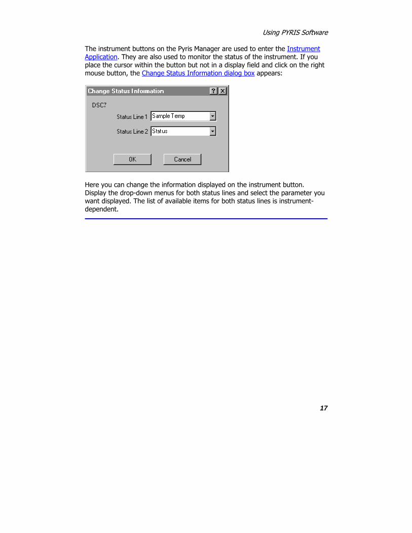
The instrument buttons on the Pyris Manager are used to enter the Instrument Application. They are also used to monitor the status of the instrument. If you place the cursor within the button but not in a display field and click on the right mouse button, the Change Status Information dialog box appears:

Here you can change the information displayed on the instrument button. Display the drop-down menus for both status lines and select the parameter you want displayed. The list of available items for both status lines is instrument-dependent.

Pyris

18

Navigating in Pyris Software for Windows

It is easy to navigate around Pyris Software for Windows' components. You can go from Instrument Viewer to Method Editor to Data Analysis and other parts by a click of the mouse on the standard toobar. The first four buttons on the standard toolbar are used to navigate between the four major parts of Pyris.

When a window such as Pyris Player or Calibration displays tabs, indicating that there are pages that make up the window, click on the tab to display the page on top of the other pages.

Another way to navigate is the use of the menu bar. Each menu item contains a specific drop-down list dependent on the analyzer and the window displayed.

19

Instrument Configuration

Pyris

20

Sapphire DSC Configuration

The Sapphire DSC Configuration dialog box appears when you select the Edit button in the Pyris Configuration dialog box when the Sapphire DSC analyzer is highlighted in the Analyzers list. It is also displayed when there is a Sapphire DSC attached to the computer and it is detected by the Pyris software when you select the Add button in the Add Analyzer dialog box. The analyzer must be powered on when you configure it into the system or it will not be recognized when you select the Add button. The fields in this dialog box are as follows: Name

If you are adding a new Sapphire DSC, the system will display a default name in this field. Type the name you wish to assign to the analyzer, using a maximum of eight characters. The name identifies the analyzer in Pyris Software for Windows; it also appears in the Instrument button on the Pyris Manager panel and in the title bar of the Instrument Application. Port

Displays the COM port to which the analyzer is attached and that you selected in the Add Analyzer dialog box. Serial Number

You can enter the serial number of the analyzer for further identification; it is not a required entry. Accessories

Lists the available accessories for the Sapphire DSC. The first selection is for the purge gas accessory. Click on the drop-down arrow to display the available choices:

Air Cooling Unit: Select this accessory if an Air Cooling Unit is attached to your analyzer. Firmware Version

Displays the version of firmware in the analyzer.


21

Diamond TMA Configuration

The Diamond TMA Configuration dialog box appears when you select the Edit button in the Pyris Configuration dialog box when the Diamond TMA analyzer is highlighted in the Analyzers list. It is also displayed when there is a Diamond TMA attached to the computer and it is detected by the Pyris software when you select the Add button in the Add Analyzer dialog box. The analyzer must be powered on when you configure it into the system or it will not be recognized when you select the Add button. The fields in this dialog box are as follows: Name

If you are adding a new Diamond TMA, the system will display a default name in this field. Type the name you wish to assign to the analyzer, using a maximum of eight characters. The name identifies the analyzer in Pyris Software for Windows; it also appears in the Instrument button on the Pyris Manager panel and in the title bar of the Instrument Application. Port



Lists the available accessories for the Diamond TMA. The first selection is for the purge gas accessory. Click on the drop-down arrow to display the available choices:

Air Cooling Unit: Select this accessory if an Air Cooling Unit is attached to your analyzer.

No Gas Accessory Firmware Version


Pyris

22


23

Diamond TG/DTA Configuration

The Diamond TG/DTA Configuration dialog box appears when you select the Edit button in the Pyris Configuration dialog box when the Diamond TG/DTA analyzer is highlighted in the Analyzers list. It is also displayed when there is a Diamond TG/DTA attached to the computer and it is detected by the Pyris software when you select the Add button in the Add Analyzer dialog box. The analyzer must be powered on when you configure it into the system or it will not be recognized when you select the Add button. The fields in this dialog box are as follows: Name

If you are adding a new Diamond TG/DTA, the system will display a default name in this field. Type the name you wish to assign to the analyzer, using a maximum of eight characters. The name identifies the analyzer in Pyris Software for Windows; it also appears in the Instrument button on the Pyris Manager panel and in the title bar of the Instrument Application. Port



Lists the available accessories for the Diamond TG/DTA. The first selection is for the purge gas accessory. Click on the drop-down arrow to display the available choices:

Air Cooling Unit: Select this accessory if an Air Cooling Unit is attached to your analyzer.

No Gas Accessory

Autosampler: Select this accessory if the Diamond TG/DTA Autosampler is installed on your analyzer. If you connected the autosampler directly into the COM1 or COM2 port on the computer instead of to the Autosampler port on the Diamond TG/DTA, indicate that port in the Port field. Test the configuration by

Pyris

24

clicking on the Test button. The message “An autosampler was found” should be displayed if the autosampler is connected properly. Firmware Version



25

Diamond DSC Configuration

The Diamond DSC Configuration dialog box appears when you select the Edit button in the Pyris Configuration dialog box when the Diamond DSC analyzer is highlighted in the Analyzers list. It is also displayed when there is a Diamond DSC attached to the computer and it is detected by the Pyris software when you select the Add button in the Add Analyzer dialog box. The analyzer must be powered on when you configure it into the system or it will not be recognized when you select the Add button. The fields in this dialog box are as follows: Name

If you are adding a new Diamond DSC, the system will display a default name in this field. Type the name you wish to assign to the analyzer, using a maximum of eight characters. The name identifies the analyzer in Pyris Software for Windows; it also appears in the Instrument button on the Pyris Manager panel and in the title bar of the Instrument Application. Port



Lists the available accessories for the Diamond DSC. The first selection is for the purge gas accessory. Click on the drop-down arrow to display the available choices:

Thermal Analysis Gas Station (TAGS): Select this accessory if a TAGS is attached to your analyzer. The TAGS can control up to 4 purge gases. Selection of this accessory is reflected in the Gas Change box on the Program page of the Method Editor. The gas program can have the TAGS switch from one gas to another at selected times or temperatures. The flow rate can also be changed.

GSA 7 Gas Switching Accessory: Select this accessory if you are using a GSA 7. Selection of this accessory is reflected in the Gas Change box on the Program page of the Method Editor. The gas program can have the GSA 7 switch the purge gas at a selected time.

Pyris

26

No Gas Accessory

The next four accessories are

CryoFill: Click in the box if your Diamond DSC is attached to the CryoFill LN2 Cooling System for subambient operation.

High-Pressure Cell: Select this accessory if you are going to use the high-pressure cell on the Diamond DSC.

Autosampler: Select this accessory if the Diamond DSC Autosampler is installed on your analyzer. If you connected the autosampler directly into the COM1 or COM2 port on the computer instead of to the Autosampler port on the Diamond DSC, indicate that port in the Port field. Test the configuration by clicking on the Test button. The message “An autosampler was found” should be displayed if the autosampler is connected properly. Firmware Version

Displays the version of firmware in the analyzer. Update Flash EPROM

Select this button when you want to update the EPROM in the analyzer. This would occur if you receive an updated version of the software. Clicking on the button displays the Pyris Flash ROM Utility dialog box in which you select the ROM file to use for updating the Pyris EPROM. Data are then transferred from the file to the analyzer’s memory.

NOTE: Do not update the firmware at the same time that you add the analyzer to the configuration list. If you need to add the analyzer and update the firmware, first add the analyzer and close the Configuration dialog box. Then reopen the Pyris Configuration dialog box, highlight Diamond DSC's name, and click on the Edit button. Click on Update Flash EPROM.


27

Pyris 1 DSC Configuration

The Pyris 1 DSC Configuration dialog box appears when you select the Edit button in the Pyris Configuration dialog box when the Pyris 1 DSC analyzer is highlighted in the Analyzers list. It is also displayed when there is a Pyris 1 DSC attached to the computer and it is detected by the Pyris software when you select the Add button in the Add Analyzer dialog box. The analyzer must be powered on when you configure it into the system or it will not be recognized when you select the Add button. The fields in this dialog box are as follows: Name

If you are adding a new Pyris 1 DSC, the system will display a default name in this field. Type the name you wish to assign to the analyzer, using a maximum of eight characters. The name identifies the analyzer in Pyris Software for Windows; it also appears in the Instrument button on the Pyris Manager panel and in the title bar of the Instrument Application. Port


You can enter the serial number of the analyzer for further identification; it is not a required entry.

NOTE: If you are running Pyris Enhanced Security you must type in the serial number of the analyzer. Accessories

Lists the available accessories for the Pyris 1 DSC. The first selection is for the purge gas accessory. Click on the drop-down arrow to display the available choices:


GSA 7 Gas Switching Accessory: Select this accessory if you are using a GSA 7. Selection of this accessory is reflected in the Gas Change box on the Program

Pyris

28

page of the Method Editor. The gas program can have the GSA 7 switch the purge gas at a selected time.

No Gas Accessory

The next four accessories are

CryoFill: Click in the box if your Pyris 1 DSC is attached to the CryoFill LN2 Cooling System for subambient operation.

DPA 7 Photocalorimetric Accessory: This selection is grayed out because the accessory is not available for use with the Pyris 1 DSC at this time.

High-Pressure Cell: Select this accessory if you are going to use the high-pressure cell on the Pyris 1 DSC.

Autosampler: Select this accessory if the Pyris 1 DSC Autosampler is installed on your analyzer. If you connected the autosampler directly into the COM1 or COM2 port on the computer instead of to the Autosampler port on the Pyris 1 DSC, indicate that port in the Port field. Test the configuration by clicking on the Test button. The message “An autosampler was found” should be displayed if the autosampler is connected properly. Firmware Version



NOTE: Do not update the firmware at the same time that you add the analyzer to the configuration list. If you need to add the analyzer and update the firmware, first add the analyzer and close the Configuration dialog box. Then reopen the Pyris Configuration dialog box, highlight Pyris 1 DSC's name, and click on the Edit button. Click on Update Flash EPROM.


29

DSC 7 Configuration

The DSC 7 Configuration dialog box appears when you select the Edit button in the Pyris Configuration dialog box when the DSC 7 analyzer is highlighted in the Analyzers list. It is also displayed when there is a DSC 7 attached to the computer and it is detected by the Pyris software when you select the Add button in the Add Analyzer dialog box. The analyzer must be powered on when you configure it into the system; otherwise, it will not be recognized when you select the Add button. The fields in this dialog box are as follows: Name

If you are adding a DSC 7, the system will display a default name in this field. Type the name you wish to assign to the analyzer, using a maximum of eight characters. The name identifies the analyzer in Pyris Software for Windows; it also appears in the Instrument button on the Pyris Manager panel and in the title bar of the Instrument Application. Port




Lists the available accessories for the DSC 7. The first selection is for the purge gas accessory. Click on the drop-down menu arrow to display the available choices:


GSA 7 Gas Switching Accessory: Select this accessory if you are using a GSA 7. Selection of this accessory is reflected in the Gas Change box on the Program

Pyris

30

page of the Method Editor. The gas program can have the GSA 7 switch the purge gas at a selected time.

No Gas Accessory

The other accessories available for selection by clicking on the check box are

CCA 7 Controlled Cooling Accessory: The CCA 7 allows low-temperature operation of the DSC 7 to –140°C (and to –70°C with a DSC 7 Robotic System).

High-Pressure Cell: This accessory is used for performing DSC experiments at elevated pressures. It has built-in connections for a liquid cooling system such as tap water or a circulating system.

DPA 7 Photocalorimetric Accessory: The DPA 7 allows samples contained in the DSC 7 to be exposed to full spectrum or individual wavelength UV light. Pyris-controlled shutter provides reproducible exposure times. Multiple lamp source capability allows selection of the appropriate UV lamp for experiments. Selection of this accessory is reflected in the Program page of the Method Editor where the Gas Change button changes to Lamp Change.

Autosampler: Select this accessory if you are using the DSC 7 Robotic System. If you connected the autosampler directly into the COM1 or COM2 port on the computer via an RS 232 cable instead of to the AUX port on the TAC 7/DX, indicate that port in the Port field. Firmware Version



31

Pyris 6 DSC Configuration

The Pyris 6 DSC Configuration dialog box appears when you select the Edit button in the Pyris Configuration dialog box when the Pyris 6 DSC analyzer is highlighted in the Analyzers list. It is also displayed when there is a Pyris 6 DSC attached to the computer and it is detected by the Pyris software when you select the Add button in the Add Analyzer dialog box. The analyzer must be powered on when you configure it into the system; otherwise, it will not be recognized when you select the Add button. The fields in this dialog box are as follows: Name

If you are adding a Pyris 6 DSC, the system will display a default name in this field. Type the name you wish to assign to the analyzer, using a maximum of eight characters. The name identifies the analyzer in Pyris Software for Windows; it also appears in the Instrument button on the Pyris Manager panel and in the title bar of the Instrument Application. Port




Lists the available accessories for the analyzer. For the Pyris 6 DSC, the only accessory is for purge gas. Click on the drop-down arrow to display the available choices:


No Gas Accessory

Pyris

32

Autosampler: Select this accessory if the AS 6 Autosampler is installed on your analyzer. The COM port for the autosampler is the same as that for the analyzer. Test the configuration by clicking on the Test button. The message “An autosampler was found” should be displayed if the autosampler is connected properly. Firmware Version



33

Jade DSC Configuration

The Jade DSC Configuration dialog box appears when you select the Edit button in the Pyris Configuration dialog box when the Jade DSC analyzer is highlighted in the Analyzers list. It is also displayed when there is a Jade DSC attached to the computer and it is detected by the Pyris software when you select the Add button on the Add Analyzer dialog box. The analyzer must be powered on when you configure it into the system; otherwise, it will not be recognized when you select the Add button. The fields in this dialog box are as follows:

Name

If you are adding a Jade DSC, the system will display a default name in this field. Type the name you wish to assign to the analyzer, using a maximum of eight characters. The name identifies the analyzer in Pyris Software for Windows; it also appears in the Instrument button on the Pyris Manager panel and in the title bar of the Instrument Application.

Port

Displays the COM port to which the analyzer is attached and that you selected in the Add Analyzer dialog box.

Pyris

34

Serial Number


NOTE: If you are running Pyris Enhanced Security you must type in the serial number of the analyzer.

Accessories

Lists the available accessories for the analyzer. For the Jade DSC the following accessories are available:

• CryoFill - Check this option if your Jade DSC was installed with CryoFill.

• Autosampler - Check this option if you have an Autosample installed on your Jade DSC. The COM Port for the autosampler is the same as that for the analyzer. You can test the configuration by clicking on the Test button. The message “An autosampler was found” should be displayed if the autosampler is connected properly.

Firmware Version

Click on the Firmware Version button to display the version of firmware in the analyzer.


35

TGA 7 and Pyris 1 TGA Configuration

The Configuration dialog box for a TGA 7 or a Pyris 1 TGA appears when you select the Edit button in the Pyris Configuration dialog box when either analyzer is highlighted in the Analyzers list. It is also displayed when there is a TGA 7 or a Pyris 1 TGA attached to the computer and it is detected by the Pyris software when you select the Add button in the Add Analyzer dialog box. The analyzer must be powered on when you configure it into the system; otherwise, it will not be recognized when you select the Add button. The fields in this dialog box are as follows:

Pyris

36

Name

If you are adding a TGA 7, the system will display the default name TGA 7 in this field. For a Pyris 1 TGA, it assigns Pyris 1 TGA. Type the name you wish to assign to the analyzer, using a maximum of eight characters. The name identifies the analyzer in Pyris Software for Windows; it also appears in the Instrument button on the Pyris Manager panel and in the title bar of the Instrument Application. Port

Displays the COM port that you selected in the Add Analyzer dialog box to which the analyzer is attached. Serial Number



Lists the available accessories for the analyzer. For the TGA 7 and Pyris 1 TGA, the only accessory in the list is for purge gas. Click on the drop-down arrow to display the available choices:


37



No Gas Accessory Autosampler

This box appears if a Pyris 1 TGA is attached to your system. Click in the check box if an autosampler is attached to the analyzer. The Port field should be the same as that for the analyzer. Click on the Test button to have the system check for the presence of the autosamper. A clock cursor will be displayed while the system goes out and locates the autosampler. A message stating that it was found should be displayed. Firmware Version



NOTE: Do not update the firmware at the same time that you add the analyzer to the configuration list. If you need to add the analyzer and update the firmware, first add the analyzer and close the Configuration dialog box. Then reopen the Pyris Configuration dialog box, highlight Pyris 1 TGA's name, and click on the Edit button. Click on Update Flash EPROM.

Pyris

38

Pyris 6 TGA Configuration

The Pyris 6 TGA Configuration dialog box appears when you select the Edit button in the Pyris Configuration dialog box when the Pyris 6 TGA analyzer is highlighted in the Analyzers list. It is also displayed when there is a Pyris 6 TGA attached to the computer and it is detected by the Pyris software when you select the Add button in the Add Analyzer dialog box. The analyzer must be powered on when you configure it into the system; otherwise, it will not be recognized when you select the Add button. The fields in this dialog box are as follows: Name

If you are adding a Pyris 6 TGA, the system will display a default name in this field. Type the name you wish to assign to the analyzer, using a maximum of eight characters. The name identifies the analyzer in Pyris Software for Windows; it also appears in the Instrument button on the Pyris Manager panel and in the title bar of the Instrument Application. Port




Lists the available accessories for the analyzer. For the Pyris 6 TGA, the only accessory is for purge gas. Click on the drop-down arrow to display the available choices:


No Gas Accessory


39

Autosampler: Select this accessory if the AS 6 Autosampler is installed on your analyzer. The COM port for the autosampler is the same as that for the analyzer. Test the configuration by clicking on the Test button. The message “An autosampler was found” should be displayed if the autosampler is connected properly. Firmware Version


Pyris

40

TGA 7 and Pyris 1 TGA Configuration

The Configuration dialog box for a TGA 7 or a Pyris 1 TGA appears when you select the Edit button in the Pyris Configuration dialog box when either analyzer is highlighted in the Analyzers list. It is also displayed when there is a TGA 7 or a Pyris 1 TGA attached to the computer and it is detected by the Pyris software when you select the Add button in the Add Analyzer dialog box. The analyzer must be powered on when you configure it into the system; otherwise, it will not be recognized when you select the Add button. The fields in this dialog box are as follows:


41

Name

If you are adding a TGA 7, the system will display the default name TGA 7 in this field. For a Pyris 1 TGA, it assigns Pyris 1 TGA. Type the name you wish to assign to the analyzer, using a maximum of eight characters. The name identifies the analyzer in Pyris Software for Windows; it also appears in the Instrument button on the Pyris Manager panel and in the title bar of the Instrument Application. Port

Displays the COM port that you selected in the Add Analyzer dialog box to which the analyzer is attached. Serial Number



Lists the available accessories for the analyzer. For the TGA 7 and Pyris 1 TGA, the only accessory in the list is for purge gas. Click on the drop-down arrow to display the available choices:

Pyris

42



No Gas Accessory Autosampler

This box appears if a Pyris 1 TGA is attached to your system. Click in the check box if an autosampler is attached to the analyzer. The Port field should be the same as that for the analyzer. Click on the Test button to have the system check for the presence of the autosamper. A clock cursor will be displayed while the system goes out and locates the autosampler. A message stating that it was found should be displayed. Firmware Version



NOTE: Do not update the firmware at the same time that you add the analyzer to the configuration list. If you need to add the analyzer and update the firmware, first add the analyzer and close the Configuration dialog box. Then reopen the Pyris Configuration dialog box, highlight Pyris 1 TGA's name, and click on the Edit button. Click on Update Flash EPROM.


43

DMA 7e Configuration

The DMA 7e Configuration dialog box appears when you select the Edit button in the Pyris Configuration dialog box when the DMA 7e analyzer is highlighted in the Analyzers list. It is also displayed when there is a DMA 7e attached to the computer and it is detected by the Pyris software when you select the Add button in the Add Analyzer dialog box. The analyzer must be powered on when you configure it into the system; otherwise, it will not be recognized when you select the Add button. The fields in this dialog box are as follows: Name

If you are adding a DMA 7e, the system will display a default name in this field. Type the name you wish to assign to the analyzer, using a maximum of eight characters. The name identifies the analyzer in Pyris Software for Windows; it also appears in the Instrument button on the Pyris Manager panel and in the title bar of the Instrument Application. Port

Displays the COM port to which the analyzer is attached and that you selected in the Add Analyzer dialog box. Accessories

Lists the available accessories for the DMA 7e. The first selection is for the purge gas accessory. Click on the drop-down arrow to display the available choices:



No Gas Accessory Force Motor

The linear force motor in the DMA 7e provides precise control of all forces applied to the sample. The high resolution of the force motor allows for precise

Pyris

44

motor controls. There are two force motors available. Click on the appropriate radio button to indicate the force motor in your DMA 7e. The force motor in your DMA 7e cannot be changed. Furnace Size

Two types of low-mass furnace are available for the DMA 7e and each can be programmed for high and low temperatures. When combined with the appropriate cooling accessories, you can program the DMA 7e to –170°C. The low mass furnace design permits a rapid cool down at the end of the experiment. Select the size of the furnace currently installed in your DMA 7e. You can change the furnace when necessary but you must edit the configuration by changing the furnace size in this box. Firmware Version



45

TMA 7 Configuration

The TMA 7 Configuration dialog box appears when you select the Edit button in the Pyris Configuration dialog box when the TMA 7 analyzer is highlighted in the Analyzers list. It is also displayed when there is a TMA 7 attached to the computer and it is detected by the Pyris software when you select the Add button in the Add Analyzer dialog box. The analyzer must be powered on when you configure it into the system; otherwise, it will not be recognized when you select the Add button. The fields in this dialog box are as follows: Name

If you are adding a TMA 7, the system will display a default name in this field. Type the name you wish to assign to the analyzer, using a maximum of eight characters. The name identifies the analyzer in Pyris Software for Windows; it also appears in the Instrument button on the Pyris Manager panel and in the title bar of the Instrument Application. Port


Lists the available accessories for the TMA 7. The first selection is for the purge gas accessory. Click on the drop-down arrow to display the available choices:



No Gas Accessory Force Motor

The linear force motor in the TMA 7 provides precise control of all forces applied to the sample. The high resolution of the force motor allows for precise motor

Pyris

46

controls. There are two force motors available. Click on the appropriate radio button to indicate the force motor in your TMA 7. The force motor in your TMA 7 cannot be changed. Furnace Size

Two types of low-mass furnace are available for the TMA 7 and each can be programmed for high and low temperatures. When combined with the appropriate cooling accessories, you can program the TMA 7 to –170°C. The low mass furnace design permits a rapid cool down at the end of the experiment. Select the size of the furnace currently installed in your TMA 7. You can change the furnace when necessary but you must edit the configuration by changing the furnace size in this box. Firmware Version



47

DTA 7 Configuration

The DTA 7 Configuration dialog box appears when you select the Edit button in the Pyris Configuration dialog box when the DTA 7 analyzer is highlighted in the Analyzers list. It is also displayed when there is a DTA 7 attached to the computer and it is detected by the Pyris software when you select the Add button in the Add Analyzer dialog box. The analyzer must be powered on when you configure it into the system; otherwise, it will not be recognized when you select the Add button. The fields in this dialog box are as follows: Name

If you are adding a DTA 7, the system will display a default name in this field. Type the name you wish to assign to the analyzer, using a maximum of eight characters. The name identifies the analyzer in Pyris Software for Windows; it also appears in the Instrument button on the Pyris Manager panel and in the title bar of the Instrument Application. Port


Lists the available accessories for the DTA 7. The only selection is for the purge gas accessory. Click on the drop-down arrow to display the list of choices:



No Gas Accessory Firmware Version


49

Instrument Applications

Pyris

50

Diamond TMA Instrument Application

The main parts of the Diamond TMA Instrument Application are

Instrument Viewer

Method Editor

Data Analysis

Pyris Player

Status Panel

Control Panel

To move from one part of the Instrument Application to another, you can use the toolbar buttons:

Instrument Viewer

Method Editor

Data Analysis

Pyris Player

Instrument Viewer

The Instrument Viewer is a window that displays the real-time signals from the Diamond TMA as data are collected during a run. You can select the curves (signals) for display from the Curves menu. If there is no run in progress, the Instrument Viewer can be used to monitor the status of the instrument by activating Monitor from the View menu. If you click on the Reset Monitor button in the control panel, the display in the Instrument Viewer is cleared and monitoring begins again. The display of the curves can be optimized by using the rescale tools on the Rescale Tools toolbar.


51

The Instrument Viewer window contains a title bar, control box with the standard Control menu, Minimize and Maximize buttons, and a border that can be used for resizing. The curves displayed in the window can be changed by selecting items on the View, Display, and Curves menus.

Method Editor

The Diamond TMA method is a set of parameters that determine the conditions under which the system will collect data on a sample. Any number of methods can be created and stored so that the parameters can be optimized to handle different analyses. Methods are also used in play lists. The play list can be set up to run many samples using the same method via the sample group. The Method Editor comprises the following pages, each of which contains its own set of parameters:

Sample Info Page

Initial State Page

Program Page

View Program Page

Another feature of the Method Editor is the Thermal Program Window.

Data Analysis

The Data Analysis window is opened one of two ways: First, you can select Data Analysis from the Start Pyris Task menu or from the Pyris Software for Windows group in the Programs menu. The window displays the last data file displayed there. Use the options on the File menu to display data files collected by different analyzers.

Second, the Diamond TMA Data Analysis window is opened while in the

Instrument Viewer or Method Editor by selecting the Data Analysis button from the toolbar. From the Open Data File dialog box select the data file you want displayed. Use the items in the File menu to open, add, close, and save a data file, or to print the display.

Pyris

52

The View, Display, Curves, Math, and Calc menus are used to change the display and the type of curve displayed and to perform calculations on the data for additional information.

The Data Analysis window also contains the standard window items: title bar, control box with Control menu, Minimize and Maximize buttons, and a border that can be used for resizing.

Pyris Player

The Pyris Player is used to create play lists or sequences of commands that automate data collection and postrun data analysis functions. For a Diamond TMA, you can create a play list that prompts you through the steps necessary to run a sample or a series of samples (i.e., Load Sample, Start Method, Remove Sample) and then performs a series of analyses on the data files, displays the results, and prints the results. The Sample List is a good way to group similar samples together to be analyzed using the same method. The items in the Data Analysis List can take the data file from the current run, preceding play list items, and existing files and perform the same procedures that are available in regular Data Analysis in a play list.

While a play list is running, you can perform other functions on your computer or pause the play list and edit the entries below the current line. A complete history file is generated that contains the record of success or failure or each item in the list. If an error occurs, a reason is listed. There also is a sample history page that displays past and current information on the samples in the sample groups in the current play list.

The parts of Pyris Player are:

Setup Page

Edit Play List Page

View List Page

View Sample List Page

View History Page

Sample History Page


53

Player Toolbars

Top

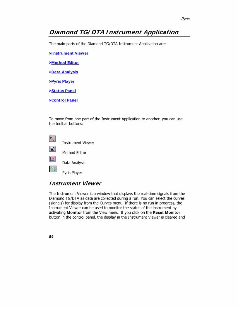
Pyris

54

Diamond TG/DTA Instrument Application

The main parts of the Diamond TG/DTA Instrument Application are:

Instrument Viewer

Method Editor

Data Analysis

Pyris Player

Status Panel

Control Panel


Instrument Viewer

Method Editor

Data Analysis

Pyris Player

Instrument Viewer

The Instrument Viewer is a window that displays the real-time signals from the Diamond TG/DTA as data are collected during a run. You can select the curves (signals) for display from the Curves menu. If there is no run in progress, the Instrument Viewer can be used to monitor the status of the instrument by activating Monitor from the View menu. If you click on the Reset Monitor button in the control panel, the display in the Instrument Viewer is cleared and


55

monitoring begins again. The display of the curves can be optimized by using the rescale tools on the Rescale Tools toolbar.


Method Editor

The Diamond TG/DTA method is a set of parameters that determine the conditions under which the system will collect data on a sample. Any number of methods can be created and stored so that the parameters can be optimized to handle different analyses. Methods are also used in play lists. The play list can be set up to run many samples using the same method via the sample group. The Method Editor comprises the following pages, each of which contains its own set of parameters:

Sample Info Page

Initial State Page

Program Page

View Program Page


Data Analysis


Second, the Diamond TG/DTA Data Analysis window is opened while in the


Pyris

56



Pyris Player

The Pyris Player is used to create play lists or sequences of commands that automate data collection and postrun data analysis functions. For a Diamond TG/DTA without an autosampler, you can create a play list that prompts you through the steps necessary to run a sample or a series of samples (i.e., Load Sample, Start Method, Remove Sample) and then performs a series of analyses on the data files, displays the results, and prints the results. If your analyzer has an autosampler, the play list's Sample Group feature, which includes a Sample List and a Data Analysis List, automates running samples in the autosampler's tray. The Sample List is a good way to group similar samples together to be analyzed using the same method. The Sample List can run the samples in the autosampler in any order. The items in the Data Analysis List can take the data file from the current run, preceding play list items, and existing files and perform the same procedures that are available in regular Data Analysis in a play list.


The parts of Pyris Player are

Setup Page

Edit Play List Page

View List Page


View History Page


57

Sample History Page

Player Toolbars

Top

Pyris

58

Diamond DSC Instrument Application

The main parts of the Diamond DSC Instrument Application are

Instrument Viewer

Method Editor

Data Analysis

Pyris Player

Status Panel

Control Panel


Instrument Viewer

Method Editor

Data Analysis

Pyris Player

Instrument Viewer

The Instrument Viewer is a window that displays the real-time signals from the Diamond DSC as data are collected during a run. You can select the curves (signals) for display from the Curves menu. If there is no run in progress, the Instrument Viewer can be used to monitor the status of the instrument by activating Monitor from the View menu. If you click on the Reset Monitor button in the control panel, the display in the Instrument Viewer is cleared and monitoring begins again. The display of the curves can be optimized by using the rescale tools on the Rescale Tools toolbar.


59


Method Editor

The Diamond DSC method is a set of parameters that determine the conditions under which the system will collect data on a sample. Any number of methods can be created and stored so that the parameters can be optimized to handle different analyses. Methods are also used in play lists. The play list can be set up to run many samples using the same method via the sample group. The Method Editor comprises the following pages, each of which contains its own set of parameters:

Sample Info Page

Initial State Page

Program Page

View Program Page


Data Analysis


Second, the Diamond DSC Data Analysis window is opened while in the


Pyris

60



Pyris Player

The Pyris Player is used to create play lists or sequences of commands that automate data collection and postrun data analysis functions. For a Diamond DSC without an autosampler, you can create a play list that prompts you through the steps necessary to run a sample or a series of samples (i.e., Load Sample, Start Method, Remove Sample) and then performs a series of analyses on the data files, displays the results, and prints the results. If your analyzer has an autosampler, the play list's Sample Group feature, which includes a Sample List and a Data Analysis List, automates running samples in the autosampler's tray. The Sample List is a good way to group similar samples together to be analyzed using the same method. The Sample List can run the samples in the autosampler in any order. The items in the Data Analysis List can take the data file from the current run, preceding play list items, and existing files and perform the same procedures that are available in regular Data Analysis in a play list.



Setup Page

Edit Play List Page

View List Page


View History Page


61

Sample History Page

Player Toolbars

Top

Pyris

62

Pyris 1 DSC Instrument Application

The main parts of the Pyris 1 DSC Instrument Application are

Instrument Viewer

Method Editor

Data Analysis

Pyris Player

Status Panel

Control Panel


Instrument Viewer

Method Editor

Data Analysis

Pyris Player

Instrument Viewer

The Instrument Viewer is a window that displays the real-time signals from the Pyris 1 DSC as data are collected during a run. You can select the curves (signals) for display from the Curves menu. If there is no run in progress, the Instrument Viewer can be used to monitor the status of the instrument by activating Monitor from the View menu. If you click on the Reset Monitor button in the control panel, the display in the Instrument Viewer is cleared and monitoring begins again. The display of the curves can be optimized by using the rescale tools on the Rescale Tools toolbar.


63


Method Editor

The Pyris 1 DSC method is a set of parameters that determine the conditions under which the system will collect data on a sample. Any number of methods can be created and stored so that the parameters can be optimized to handle different analyses. Methods are also used in play lists. The play list can be set up to run many samples using the same method via the sample group. The Method Editor comprises the following pages, each of which contains its own set of parameters:

Sample Info Page

Initial State Page

Program Page

View Program Page


Data Analysis


Second, the Pyris 1 DSC Data Analysis window is opened while in the Instrument

Viewer or Method Editor by selecting the Data Analysis button from the toolbar. From the Open Data File dialog box select the data file you want displayed. Use the items in the File menu to open, add, close, and save a data file, or to print the display.

Pyris

64



Pyris Player

The Pyris Player is used to create play lists or sequences of commands that automate data collection and postrun data analysis functions. For a Pyris 1 DSC without an autosampler, you can create a play list that prompts you through the steps necessary to run a sample or a series of samples (i.e., Load Sample, Start Method, Remove Sample) and then performs a series of analyses on the data files, displays the results, and prints the results. If your analyzer has an autosampler, the play list's Sample Group feature, which includes a Sample List and a Data Analysis List, automates running samples in the autosampler's tray. The Sample List is a good way to group similar samples together to be analyzed using the same method. The Sample List can run the samples in the autosampler in any order. The items in the Data Analysis List can take the data file from the current run, preceding play list items, and existing files and perform the same procedures that are available in regular Data Analysis in a play list.



Setup Page

Edit Play List Page

View List Page


View History Page


65

Sample History Page

Player Toolbars

Top

Pyris

66

DSC 7 Instrument Application

The main parts of the DSC 7 Instrument Application are

Instrument Viewer

Method Editor

Data Analysis

Pyris Player

Status Panel

Control Panel


Instrument Viewer

Method Editor

Data Analysis

Pyris Player

Instrument Viewer

The DSC 7 Instrument Viewer is a window that displays the real-time signals from the DSC 7 as data are collected during a run. You can select the curves (signals) for display from the Curves menu. If there is no run in progress, the Instrument Viewer can be used to monitor the status of the instrument by activating Monitor from the View menu. If you click on the Reset Monitor button in the control panel, the display in the Instrument Viewer is cleared and monitoring begins again. The display of the curves can be optimized by using the rescale tools on the Rescale Tools toolbar.


67


Method Editor

The DSC 7 method is a set of parameters that determine the conditions under which the system will collect data on a sample. Any number of methods can be created and stored so that the parameters can be optimized to handle different analyses. Methods are also used in play lists. The play list can be set up to run many samples using the same method via the sample group. The Method Editor comprises the following pages, each of which contains its own set of parameters:

Sample Info Page

Initial State Page

Program Page


Data Analysis


Second, the DSC 7 Data Analysis window is opened while in the Instrument

Viewer or Method Editor by selecting the Data Analysis button from the toolbar. From the Open Data File dialog box select the data file that you want displayed. Use the items in the File menu to open, add, close, and save a data file, or to print the display.


Pyris

68


Pyris Player

The Pyris Player is used to create play lists or sequences of commands that automate data collection and postrun data analysis functions. For a DSC 7 without a Robotic System, you can create a play list that prompts you through the steps necessary to run a sample or a series of samples (i.e., Load Sample, Start Method, Remove Sample) and then performs a series of analyses on the data files, displays the results, and prints the results. If your analyzer has a Robotic System, the play list's Sample Group feature, which includes a Sample List and a Data Analysis List, automates running samples in the autosampler's tray. The Sample List is a good way to group similar samples together to be analyzed by the same method. The samples you enter in the list can be in any order in the autosampler tray. The items in the Data Analysis List can take the data file from the current run, preceding play list items, and existing files and perform the same procedures that are available in regular Data Analysis in a play list.

While a play list is running, you can perform other functions on your computer or pause the play list and edit the entries below the current line. A complete history file is generated that contains the record of success or failure of each item in the list. If an error occurs, a reason is listed. There also is a sample history page that displays past and current information on the samples in the Sample Lists in the current play list.

The parts of Pyris Player are Setup Page

Edit Play List Page

View List Page


View History Page

Sample History Page

Player Toolbars

Top


69

Pyris 6 DSC Instrument Application

The main parts of the Pyris 6 DSC Instrument Application are

Instrument Viewer

Method Editor

Data Analysis

Pyris Player

Status Panel

Control Panel


Instrument Viewer

Method Editor

Data Analysis

Pyris Player

Instrument Viewer

The Instrument Viewer is a window that displays the real-time signals from the Pyris 6 DSC as data are collected during a run. You can select the curves (signals) for display from the Curves menu. If there is no run in progress, the Instrument Viewer can be used to monitor the status of the instrument by activating Monitor from the View menu. If you click on the Reset Monitor button in the control panel, the display in the Instrument Viewer is cleared and monitoring begins again. The display of the curves can be optimized by using the rescale tools on the Rescale Tools toolbar.

Pyris

70


Method Editor

The Pyris 6 DSC method is a set of parameters that determine the conditions under which the system will collect data on a sample. Any number of methods can be created and stored so that the parameters can be optimized to handle different analyses. Methods are also used in play lists. The play list can be set up to run many samples using the same method via the sample group. The Method Editor comprises the following pages, each of which contains its own set of parameters:

Sample Info Page

Initial State Page

Program Page

View Program Page


Data Analysis


Second, the Pyris 6 DSC Data Analysis window is opened while in the Instrument

Viewer or Method Editor by selecting the Data Analysis button from the toolbar. From the Open Data File dialog box sselect the data file you want displayed. Use the items in the File menu to open, add, close, and save a data file or to print the display.

The View, Display, Curves, Math, and Calc menus are used to change the display and the type of curve and to perform calculations on the data for additional information.


71


Pyris Player

Pyris Player is used to create play lists or sequences of commands that automate data collection and postrun data analysis functions. You can create a play list that prompts you through the steps necessary ro run a sample or a series of samples (i.e., Load Sample, Start Method, Remove Sample) and then performs a series of analyses on the data files, displays the results, and prints the results. Pyris Player's Sample Group feature, which includes a Sample List and a Data Analysis List, simplifies creation of a play list. For each Sample line in the Sample List, the program will pause in order for you to load or remove the sample since it does not detect an autosampler. The Sample List is a good way to group similar samples together to be analyzed by the same method. The items in the Data Analysis List can take the data file from the current run, preceding play list items, and existing files and perform the same procedures that are available in regular Data Analysis in a play list.

While a play list is running, you can perform other functions on your computer or pause the play list to edit entries below the current line. A complete history file is generated that contains the record of success or failure of each item in the list. If an error occurs, a reason is listed. There also is a sample history page that displays past and current information on the samples in the Sample Lists in the current play list.

See the following topics for more details on the parts of Pyris Player: Setup Page

Edit Play List Page

View List Page


View History Page

Sample History Page

Player Toolbars

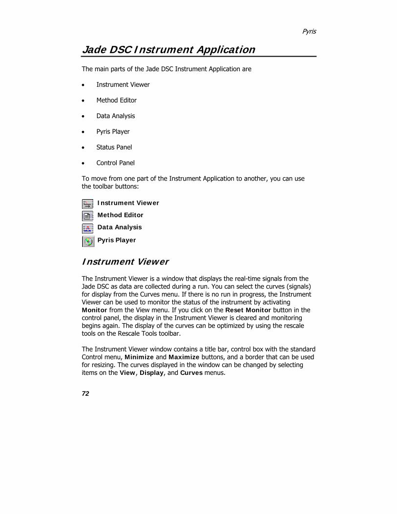
Pyris

72

Jade DSC Instrument Application

The main parts of the Jade DSC Instrument Application are

• Instrument Viewer

• Method Editor

• Data Analysis

• Pyris Player

• Status Panel

• Control Panel


Instrument Viewer

Method Editor

Data Analysis

Pyris Player

Instrument Viewer

The Instrument Viewer is a window that displays the real-time signals from the Jade DSC as data are collected during a run. You can select the curves (signals) for display from the Curves menu. If there is no run in progress, the Instrument Viewer can be used to monitor the status of the instrument by activating Monitor from the View menu. If you click on the Reset Monitor button in the control panel, the display in the Instrument Viewer is cleared and monitoring begins again. The display of the curves can be optimized by using the rescale tools on the Rescale Tools toolbar. The Instrument Viewer window contains a title bar, control box with the standard Control menu, Minimize and Maximize buttons, and a border that can be used for resizing. The curves displayed in the window can be changed by selecting items on the View, Display, and Curves menus.


73

Method Editor

The Jade DSC method is a set of parameters that determine the conditions under which the system will collect data on a sample. Any number of methods can be created and stored so that the parameters can be optimized to handle different analyses. Methods are also used in play lists. The play list can be set up to run many samples using the same method via the sample group. The Method Editor comprises the following pages, each of which contains its own set of parameters:

• Sample Info Page

• Initial State Page

• Program Page

• View Program Page


Data Analysis

This application analyzes data collected by any analyzer. This application is not associated with a particular analyzer and can be used to analyze data and edit methods for any instrument attached to your thermal analysis system. More than one Data Analysis Application can be opened at a time.

The Data Analysis window is opened one of two ways:

• From the Start Pyris menu select Data Analysis. The Data Analysis window appears.

• Use the options on the File menu to display data files collected by different analyzers.

• You can also open the Jade DSC Data Analysis window while in the Instrument Viewer or Method Editor by selecting the Data Analysis

tool bar icon . From the Open Data File dialog box select the data file you want displayed.

Pyris

74

• Use the items in the File menu to open, add, close, and save a data file or to print the display.

The View, Display, Curves, Math, and Calc menus are used to change the display and the type of curve and to perform calculations on the data for additional information.


Pyris Player

Pyris Player is used to create play lists or sequences of commands that automate data collection and postrun data analysis functions. You can create a play list that prompts you through the steps necessary ro run a sample or a series of samples (i.e., Load Sample, Start Method, Remove Sample) and then performs a series of analyses on the data files, displays the results, and prints the results. Pyris Player's Sample Group feature, which includes a Sample List and a Data Analysis List, simplifies creation of a play list. For each Sample line in the Sample List, the program will pause in order for you to load or remove the sample since it does not detect an autosampler. The Sample List is a good way to group similar samples together to be analyzed by the same method. The items in the Data Analysis List can take the data file from the current run, preceding play list items, and existing files and perform the same procedures that are available in regular Data Analysis in a play list. While a play list is running, you can perform other functions on your computer or pause the play list to edit entries below the current line. A complete history file is generated that contains the record of success or failure of each item in the list. If an error occurs, a reason is listed. There also is a sample history page that displays past and current information on the samples in the Sample Lists in the current play list. See the following topics for more details on the parts of Pyris Player:

• Setup Page

• Edit Play List Page

• View List Page

• View Sample List Page


75

• View History Page

• Sample History Page

• Player Toolbars

Pyris

76

TGA 7 Instrument Application

To learn more about the main parts of the TGA 7 Instrument Application, see each of the topics below:

Instrument Viewer

Method Editor

Data Analysis

Pyris Player

Status Panel

Control Panel


Instrument Viewer

Method Editor

Data Analysis

Pyris Player

Instrument Viewer

The TGA 7 Instrument Viewer is a window that displays the real-time signals from the TGA 7 as data are collected during a run. You can select the curves (signals) for display from the Curves menu. If there is no run in progress, the Instrument Viewer can be used to monitor the status of the instrument by activating Monitor from the View menu. If you click on the Reset Monitor button in the Control Panel, the display in the Instrument Viewer is cleared and


77

monitoring begins again. The display of the curves can be optimized by using the rescale tools on the Rescale Tools toolbar.


Method Editor

The TGA 7 method is a set of parameters that determine the conditions under which the system will collect data on a sample. Any number of methods can be created and stored so that the parameters can be optimized to handle different analyses. Methods are also used in play lists. The play list can be set up to run many samples using the same method via the sample group. The Method Editor comprises the following pages, each of which contains its own set of parameters:

Sample Info Page

Initial State Page

Program Page

View Program Page


Data Analysis

The Data Analysis window is opened one of two ways: First, you can select Data Analysis from the Start Pyris Task menu or from the Pyris Software for Windows group in the Program menu. The window displays the last data file displayed there. Use the options on the File menu to display data files collected by different analyzers.

Second, the instrument's Data Analysis window is opened while in the

Instrument Viewer or Method Editor by selecting the Data Analysis button from the toolbar. From the Open Data File dialog box select the data file you want displayed. Use the items in the File menu to open, add, close, and save a data file, or to print the display. The View, Display, Curves, Math, and Calc menus are used to change the display and the type of curve displayed and to perform calculations on the data for additional information.

Pyris

78


Pyris Player

The Pyris Player is used to create play lists or sequences of commands that automate data collection and postrun data analysis functions. You can create a play list that prompts you through the steps necessary to run a sample or a series of samples (i.e., Load Sample, Start Method, Remove Sample) and then performs a series of analyses on the data files, displays the results, and prints the results. Pyris Player's Sample Group feature, which includes a Sample List and a Data Analysis List, simplifies creation of a play list. For each Sample line in the Sample List, the program will pause in order for you to load or remove a sample since it does not detect an autosampler. The Sample List is a good way to group similar samples together to be analyzed using the same method. The items in the Data Analysis List can take the data file from the current run, preceding play list items, and existing files and perform the same procedures thar are available in regular Data Analysis in a play list.

While a play list is running, you can perform other functions on your computer or pause the play list to edit entries below the current line. A complete history file is generated that contains the record of success or failure of each item in the list. If an error occurs, a reason is listed. There also is a sample history page that displays past and current information on the samples in the Samples Lists in current play list.


Edit Play List Page

View List Page


View History Page

Sample History Page

Player Toolbars

Top


79

Pyris 6 TGA Instrument Application

The main parts of the Pyris 6 TGA Instrument Application are

Instrument Viewer

Method Editor

Data Analysis

Pyris Player

Status Panel

Control Panel


Instrument Viewer

Method Editor

Data Analysis

Pyris Player

Instrument Viewer

The Instrument Viewer is a window that displays the real-time signals from the Pyris 6 TGA as data are collected during a run. You can select the curves (signals) for display from the Curves menu. If there is no run in progress, the Instrument Viewer can be used to monitor the status of the instrument by activating Monitor from the View menu. If you click on the Reset Monitor button in the control panel, the display in the Instrument Viewer is cleared and monitoring begins again. The display of the curves can be optimized by using the rescale tools on the Rescale Tools toolbar.

Pyris

80


Method Editor

The Pyris 6 TGA method is a set of parameters that determine the conditions under which the system will collect data on a sample. Any number of methods can be created and stored so that the parameters can be optimized to handle different analyses. Methods are also used in play lists. The play list can be set up to run many samples using the same method via the sample group. The Method Editor comprises the following pages, each of which contains its own set of parameters:

Sample Info Page

Initial State Page

Program Page

View Program Page


Data Analysis


Second, the instrument's Data Analysis window is opened while in Instrument




81


Pyris Player

The Pyris Player is used to create play lists or sequences of commands that automate data collection and postrun data analysis functions. You can create a play list that prompts you through the steps necessary to run a sample or a series of samples (i.e., Load Sample, Start Method, Remove Sample) and then performs a series of analyses on the data files, displays the results, and prints the results. Pyris Player's Sample Group feature, which includes a Sample List and a Data Analysis List, simplifies creation of a play list. For each Sample line in the Sample List, the program will pause in order for you to load or remove the sample since it does not detect an autosampler. The Sample List is a good way to group similar samples together to be analyzed by the same method. The items in the Data Analysis List can take the data file from the current run, preceding play list items, and existing files and perform the same procedures that are available in regular Data Analysis in a play list.

While a play list is running, you can perform other functions on your computer or pause the play list to edit entries below the current line. A complete history file is generated that contains the record of success or failure of each item in the list. If an error occurs, a reason is listed. There also is a sample history page that displays past and current information on the samples in the Sample Lists in current play list.


Edit Play List Page

View List Page


Sample History Page

View History Page

Player Toolbars

Top

Pyris

82

Pyris 1 TGA Instrument Application

To learn more about the main parts of the Pyris 1 TGA Instrument Application, see each of the topics below:

Instrument Viewer

Method Editor

Data Analysis

Pyris Player

Status Panel

Control Panel


Instrument Viewer

Method Editor

Data Analysis

Pyris Player

Instrument Viewer

The Pyris 1 TGA Instrument Viewer is a window that displays the real-time signals from the Pyris 1 TGA as data are collected during a run. You can select the curves (signals) for display from the Curves menu. If there is no run in progress, the Instrument Vieweer can be used to monitor the status of the instrument by activating Monitor from the View menu. If you click on the Reset Monitor button in the control panel, the display in the Instrument Viewer is


83

cleared and monitoring begins again. The display of the curves can be optimized by using the rescale tools on the Rescale Tools toolbar.

The Instrument Viewer window contains a title bar, control box with the standard Control menu in the upper-left-hand corner, Minimize and Maximize buttons, and a border that can be used for resizing. The curves displayed in the window can be changed by selecting items on the View, Display, and Curves menus.

Method Editor

The Pyris 1 TGA method is a set of parameters that determine the conditions under which the system will collect data on a sample. Any number of methods can be created and stored so that the parameters can be optimized to handle different analyses. Methods are also used in play lists. The play list can be set up to run many samples using the same method via the sample group. This is especially convenient for use with the autosampler. The Method Editor comprises the following pages, each of which contains its own set of parameters:

Sample Info Page

Initial State Page

Program Page

View Program Page


Data Analysis

The Data Analysis window is opened one of two ways: First, you can select Data Analysis from the Start Pyris Task menu or from the Pyris Software for Windows group in the Program menu. The window displays the last data file displayed there. Use the options on the File menu to display data files collected by different analyzers.

Second, the instrument's Data Analysis window is opened while in the Instrument Viewer or Method Editor by selecting the Data Analysis button from the toolbar. From the Open Data File dialog box select the data file you want displayed. Use the items in the File menu to open, add, close, and save a data file, or to print the display. The View, Display, Curves, Math, and Calc menus are used to change the display and the type of curve displayed and to perform calculations on the data for additional information.

Pyris

84

The Data Analysis window also contains the standard window items: title bar, control box with Control menu in the upper-left-hand corner, Minimize and Maximize buttons, and a border that can be used for resizing.

Pyris Player

The Pyris Player is used to create play lists or sequences of commands that automate data collection and postrun data analysis functions. For a Pyris 1 TGA without an autosampler, you can create a play list that prompts you through the steps necessary to run a sample or a series of samples (i.e., Load Sample, Start Method, Remove Sample) and then performs a series of analyses on the data files, displays the results, and prints the results. If your analyzer has an autosampler, Pyris Player can be used to tare all or specific sample pans and weigh all or specific samples in the autosampler tray. Pyris Player's Sample Group feature, which includes a Sample List and a Data Analysis List, automates running samples in the autosampler tray. The Sample List is a good way to group similar samples together to be analyzed by the same method. The Sample List can run the samples in the autosampler in any order. The items in the Data Analysis List can take the data file from the current run, preceding play list items, and existing files and perform the same procedures that are available in regular Data Analysis in a play list.



Edit Play List Page

View List Page


View History Page

Sample History Page

Player Toolbars

Top


85

DMA 7e Instrument Application

The main parts of the DMA 7e Instrument Application are

Instrument Viewer

Method Editor

Data Analysis

Pyris Player

Status Panel

Control Panel


Instrument Viewer

Method Editor

Data Analysis

Pyris Player

Instrument Viewer

The Instrument Viewer is a window that displays the real-time signals from the DMA 7e as data are collected during a run. You can select the curves (signals) for display from the Curves menu. If there is no run in progress, the Instrument Viewer can be used to monitor the status of the instrument by activating Monitor from the View menu. If you click on the Reset Monitor button in the control panel, the display in the Instrument Viewer is cleared and monitoring begins again. The display of the curves can be optimized by using the rescale tools on the Rescale Tools toolbar.

Pyris

86


Method Editor

The DMA 7e method is a set of parameters that determine the conditions under which the system will collect data on a sample. Any number of methods can be created and stored so that the parameters can be optimized to handle different analyses. Methods are also used in play lists. The play list can be set up to run many samples using the same method via the sample group. The Method Editor comprises the following pages, each of which contains its own set of parameters:

Sample Info Page

Initial State Page

Program Page

View Program Page

Another feature of Method Editor is the Thermal Program Window.

Data Analysis



Instrument Viewer or Method Editor by selecting the Data Analysis button from the toolbar. Use the items in the File menu to open, add, close, and save a data file, or to print the display.



87

The Data Analysis window also contains the standard window items: title bar, control box with Control menu, Minimize and Maximize buttons, and a border that can be used for sizing.

Pyris Player

The Pyris Player is used to create play lists or sequences of commands that automate data collection and postrun data analysis functions. You can create a play list that prompts you through the steps necessary to run a sample or a series of samples (i.e., Load Sample, Start Method, Unload Sample) and then performs a series of analyses on the data files, displays the results, and prints the results. Pyris Player's Sample Group feature, which includes a Sample List and a Data Analysis List, simplifies creation of a play list. For each Sample line in the Sample List, the program will pause in order for you to load or remove the sample since it does not detect an autosampler. The Sample List is a good way to group similar samples together to be analyzed using the same method. The items in the Data Analysis List can take the data file from the current run, preceding play list items, and existing files and perform the same procedures that are available in regular Data Analysis in a play list.



Edit Play List Page

View List Page


View History Page

Sample History Page

Player Toolbars

Top

Pyris

88

TMA 7 Instrument Application

The main parts of the TMA 7 Instrument Application are

Instrument Viewer

Method Editor

Data Analysis

Pyris Player

Status Panel

Control Panel


Instrument Viewer

Method Editor

Data Analysis

Pyris Player

Instrument Viewer

The Instrument Viewer is a window that displays the real-time signals from the TMA 7 as data are collected during a run. You can select the curves (signals) for display from the Curves menu. If there is no run in progress, the Instrument Viewer can be used to monitor the status of the instrument by activating Monitor from the View menu. If you click on the Reset Monitor button in the control panel, the display in the Instrument Viewer is cleared and monitoring begins again. The display of the curves can be optimized by using the rescale tools on the Rescale Tools toolbar.


89


Method Editor

The TMA 7 method is a set of parameters that determine the conditions under which the system will collect data on a sample. Any number of methods can be created and stored so that the parameters can be optimized to handle different analyses. Methods are also used in play lists. The play list can be set up to run many samples using the same method via the sample group. The Method Editor comprises the following pages, each of which contains its own set of parameters:

Sample Info Page

Initial State Page

Program Page

View Program Page


Data Analysis

The Data Analysis window is opened in one of two ways: First, you can select Data Analysis from the Start Pyris Task menu or from the Pyris Software for Windows group in the Programs menu. The window displays the last data file displayed there. Use the options on the File menu to display data files collected by different analyzers.




Pyris

90


Pyris Player

The Pyris Player allows you to create play lists or sequences of commands that automate postrun data analysis functions. You can create lists that display data curves; perform calculations on the curves; delete, copy, or save curves; and print results. Pyris Player also has a feature with which you can group samples together to be run by the same method and analyzed by the same data analysis procedures. While a play list is running, you can perform other functions on your computer or edit the currently running play list. If a run is in progress, you can pause the play list to edit entries in the play list that follow the current line. A complete history file is generated for a play list. It contains the record of success or failure of each item in the list. If an error occurs, a reason is listed. There also is a sample history that displays past and current information on samples in a sample group.


Edit Play List Page

View List Page


View History Page

Sample History Page

Player Toolbars

Top


91

DDSC Instrument Application

The main parts of the DDSC Instrument Application are

Instrument Viewer

Method Editor

Data Analysis

Pyris Player

Status Panel

Control Panel


Instrument Viewer

Method Editor

Data Analysis

Pyris Player

Instrument Viewer

The Instrument Viewer is a window that displays the real-time signals from the DDSC as data are collected during a run. You can select the curves (signals) for display from the Curves menu. If there is no run in progress, the Instrument Viewer can be used to monitor the status of the instrument by activating Monitor from the View menu. If you click on the Reset Monitor button in the Control Panel, the display in the Instrument Viewer is cleared and monitoring begins again. The display of the curves can be optimized by using the rescale tools on the Rescale Tools toolbar.

Pyris

92


Method Editor

The DDSC method is a set of parameters that determine the conditions under which the system will collect data on a sample. Any number of methods can be created and stored so that the parameters can be optimized to handle different analyses. Methods are also used in play lists. The play list can be set up to run many samples using the same method via the sample group. The Method Editor comprises the following pages, each of which contains its own set of parameters:

Sample Info Page

Initial State Page

Program Page

View Program Page


Data Analysis


Second, the instrument's Data Analysis window is opened while in Instrument




93


Pyris Player

The Pyris Player for the DDSC on the DSC 7 or the Pyris 1 DSC allows you to create play lists or sequences of commands that automate postrun data analysis functions. You can create lists that display data curves; perform calculations on the curves; delete, copy, or save curves; and print results. You can also create a play list to run samples using different methods or group the samples using the same method and analyzed by the same data analysis procedures. While a play list is running, you can perform other functions on your computer or edit the currently running play list. If a run is in progress, you can pause the play list to edit entries in the play list that follow the current line. A complete history file is generated for a play list. It contains the record of success or failure of each item in the list. If an error occurs, a reason is listed. There is also a sample history that displays past and current information on samples in a sample group.


Edit Play List Page

View List Page


View History Page

Sample History Page

Player Toolbars

Top

Pyris

94

DTA 7 Instrument Application

The main parts of the DTA 7 Instrument Application are

Instrument Viewer

Method Editor

Data Analysis

Pyris Player

Status Panel

Control Panel


Instrument Viewer

Method Editor

Data Analysis

Pyris Player

Instrument Viewer

The Instrument Viewer is a window that displays the real-time signals from the DTA 7 as data are collected during a run. You can select the curves (signals) for display from the Curves menu. If there is no run in progress, the Instrument Viewer can be used to monitor the status of the instrument by activating Monitor from the View menu. If you click on the Reset Monitor button in the Control Panel, the display in the Instrument Viewer is cleared and monitoring begins again. The display of the curves can be optimized by using the rescale tools on the Rescale Tools toolbar.


95


Method Editor

The DTA 7 method is a set of parameters that determine the conditions under which the system will collect data on a sample. Any number of methods can be created and stored so that the parameters can be optimized to handle different analyses. Methods are also used in play lists. The play list can be set up to run many samples using the same method via the sample group. The Method Editor comprises the following pages, each of which contains its own set of parameters:

Sample Info Page

Initial State Page

Program Page

View Program Page


Data Analysis



Instrument Viewer or Method Editor by selecting the Data Analysis button from the toolbar. From the Open Data File dialog box, select the data file you want displayed. Use the items in the File menu to open, add, close, and save a data file, or to print the display.


Pyris

96


Pyris Player

The Pyris Player is used to create play lists or sequences of commands that automate data collection and postrun data analysis functions. You can create a play list that prompts you through the steps necessary to run a sample or a series of samples (i.e., Load Sample, Start Method, Remove Sample) and then performs a series of analyses on the data files, displays the results, and prints the results. Pyris Player's Sample Group feature, which includes a Sample List and a Data Analysis List, simplifies creation of a play list. For each Sample line in the Sample List, the program will pause in order for you to load or remove the sample since it does not detect an autosampler. The Sample List is a good way to group similar samples together to be analyzed by the same method. The items in the Data Analysis List can take the data file from the current run, preceding play list items, and existing files and perform the same procedures that are available in regular Data Analysis in a play list.



Edit Play List Page

View List Page


View History Page

Sample History Page

Player Toolbars

Top


97

Status Panel

The status panel is a dockable panel in an Instrument Application that displays the real-time status of selected parameters of the analyzer. For example, if you click on the Zero Height button on the DMA 7e control panel, the reading is displayed in the Probe Position box in the status panel.

The panel is resizable so that you can display as many parameter boxes as desired. You can toggle the status panel on and off by selecting Status Panel from the View menu. Each parameter is displayed in a box that contains the parameter name in a drop-down list and the current value.

The parameters available for display depend on the analyzer you are using. To select a parameter to display in the status panel, you can highlight the display field and then type in the first letter of the parameter. This will display the first parameter that begins with that letter. Continue to type that letter to scroll through all parameters that begin with that letter. For example, for the DTA 7, if you type the letter “f” when a status panel display field is highlighted, you will scroll through Furnace Cover, Furnace Lock, Furnace Status, and Furnace Temperature. You can also select a parameter by displaying the drop-down list and highlighting the desired item.

99

Files

Pyris

100

Pyris Files

All methods, collected data, analyzed data, calibration values, and play lists are stored by Pyris Software for Windows as files on your computer or network. You can open and close, save, delete, rename, copy, or move any of the files you use with Pyris Software for Windows.

These are the four types of Pyris files:

Method Files

A method contains all of the experimental parameters for a sample run. It is stored on your computer or network as a file and can be recalled for later use. To use a method for a sample run, select Open Method from the File menu in Instrument Application. Choose the desired method file from the displayed dialog box. The default directory for method files is C:\Program Files\Pyris\Methods. You can then edit the method, create a new method based on the open method, and start a run using the current method.

Data Files

Data collected during a sample run is stored on your computer or network as a data file. The name and location of the data file are specified in the method used for that sample run. The default directory for data files is C:\Program Files\Pyris\Data. To analyze previously collected and stored data, activate Data Analysis by selecting the Data Analysis button on the toolbar, by selecting it from the Start Pyris Task menu, or by selecting Data Analysis from the Pyris Software for Windows folder in the Programs menu. Select a specific data file from the dialog box displayed. You can open another data file by selecting Open Data from the File menu.

Calibration Files

The values used to calibrate a Pyris analyzer can be stored on your computer or network as a calibration file and recalled for later use.

Play List Files

The play lists you create in Pyris Player can be stored on your computer or network as play list files and recalled for later use or editing. A play list contains a sequence of commands that automate runs on instruments with autosamplers. Play lists also can be used with analyzers without an autosampler for automating postrun data analysis.

Calibration files overview

101

You can also import data files from 7 Series/UNIX instruments or from PC Series instruments with the data conversion software.

Pyris

102

Calibration Files

Calibration files have the following file name extensions: Diamond TG/DTA Data: .tdtc Diamond TMA Data: dtmc Diamond TMA High Temp Data: .dthc Pyris 1 DSC Data: .dcc Pyris 6 DSC/Jade DSC Data: .d6c Sapphire DSC Data: .drdc Pyris 1 TGA Data: .tg1c Pyris 6 TGA Data: .t6c DMA 7e Data: .dmc Diamond DSC Data: .pdic

File Location

You can save your calibration files anywhere on your computer or network. The default directory is C:\Program Files\Pyris\Calibrations. Multiple calibration files can be saved for different analyzer conditions.

NOTE: If you are using Pyris Enhanced Security you are restricted to saving files according to the directory paths set by an Administrator.

NOTE: If you are upgrading your Pyris Software for Windows, your old calibration files, which were saved in the default C:\PE\PYRIS subdirectory, are still in that directory and are available for your use.

103

Data Files

Data files have the following file name extensions: Diamond TG/DTA Data: .tdtm Diamond TMA Data: dtmm Diamond TMA High Temp Data: .dthm Pyris 1 DSC Data: .dcd Pyris 6 DSC/Jade DSC Data: .d6d Sapphire DSC Data: .drdm Pyris 1 TGA Data: .tg1m Pyris 6 TGA Data: .t6d DMA 7e Data: .dmd Diamond DSC Data: .pdim

File Name Format

If a method in a Pyris Player play list is used for more than one sample, or if you use the Sample List feature in Pyris Player, e.g., in a Sample Group for an autosampler, enter a file name with the format <user-defined name>###. The ### tells the software to append a number, starting with 000, to the end of the file name. The software pads the number with zeros to the left as needed. If you enter a file name in the File Name field in the Sample Info page of a method or in a Pyris Player play list and use these symbols, then each time the method is run, the software increments the file name by 1. If you do not enter # signs at the end of the user-defined part of a file name and the method is used in a play list, or even when used in a stand-alone manner, the software will append a date – time stamp to the user-defined file name to create a unique file name for each run. The format of the file name is <user-defined name>@YYMMDDHHMMSS.xxD, where YY is the year, MM the month, DD the day, HH the hour (on a 24-hour clock), MM minutes, and SS seconds.

File Location

You can save your data files anywhere on your computer or network. During software installation, you can accept the default directory for the software files, i.e., C:\Program Files\Pyris. This also means that data files are stored in C:\Program Files\Pyris\Data. You can identify a different default directory during installation of Pyris Software for Windows. The default directory can be changed in the Save page of the Preferences dialog.


Pyris

104

NOTE: If you are upgrading your Pyris Software for Windows, your old data files, which were saved in the default C:\PE\PYRIS\DATA subdirectory, are still in that directory and are available for your use.

105

Method Files

Method files have the following file name extensions: Diamond TMA Standard Methods: .dtmm Diamond TMA High Temperature Methods: .dthm Diamond TG/DTA Methods: .tdtm DSC 7 Methods: .dsm DDSC Methods: .ddm Pyris 1 DSC Methods: .dcm Pyris 6 DSC Methods/Jade DSC Methods: .d6m TGA 7 Methods: .tgm High Temperature TGA 7 Methods: .thm Pyris 6 TGA Methods: .t6m Pyris 1 TGA Methods: .tg1m High Temperature Pyris 1 TGA Methods: .th1m DMA 7e Methods: .dmm DMA 7e (28-mm Furnace) Methods: .d8m TMA 7 Methods: .tmm TMA 7 (28-mm Furnace) Methods: .t8m DTA 7 Methods: .dtm

File Location

You can save your method files anywhere on your computer or network. During software installation, you can accept the default directory for the software files, i.e., C:\Program Files\Pyris. This also means that method files are stored in C:\Program Files\Pyris\Methods. You can identify a different default directory during installation of Pyris Software for Windows. The default directory can be changed in the Save page of Preferences.


NOTE: If you are upgrading your Pyris Software for Windows, your old method files, which were saved in the default C:\PE\PYRIS\METHODS subdirectory, are still in that directory and are available for your use.

107

Play List Files

Play list files have the following three-character file name extensions: Diamond TMA Standard Play List: .dtmp Diamond TMA High Temperature Play List: .dthp Diamond TG/DTA Play List: .tdtp DSC 7 Play List: .dsp DDSC Play List: .ddp Pyris 1 DSC Play List: .dcp Pyris 6 DSC Play List: .d6p TGA 7 Play List: .tgp High Temperature TGA 7 Play List: .thp Pyris 6 TGA Play List: .t6p Pyris 1 TGA Play List: .tg1p High Temperature Pyris 1 TGA Play List: .th1p DMA 7e Play List: .dmp DMA 7e (28-mm Furnace) Play List: .d8p TMA 7 Play List: .tmp TMA 7 (28-mm Furnace) Play List: .t8p DTA 7 Play List: .dtp

File Location

You can save your play list files anywhere on your computer or network. During software installation, you can accept the default directory for the software files, i.e., C:\Program Files\Pyris. This also means that play list files are stored in C:\Program Files\Pyris\Player Lists. You can identify a different default directory during installation of Pyris Software for Windows. The default directory can be changed in the Save page of Preferences.


NOTE: If you are upgrading your Pyris Software for Windows, your old play list files, which were saved in the default C:\PE\PYRIS\PLAY LISTS subdirectory, are still in that directory and are available for your use.

Pyris

108

Data File Conversion

Data collected by 7 Series/UNIX analyzers can be imported to your Pyris system and converted for analysis by using the Pyris Import and Export utilities. To convert non-Pyris data files to Pyris data files, perform the following steps:

Install the Export utility on the 7 Series/UNIX Workstation

Run the Export utility

Transfer the ANF files to floppy disks

Transfer the ANF files to the Pyris Software for Windows workstation

Convert the ANF files to Pyris data files

Files

109

Open

Open Command

Use this command to open an existing calibration file. When you select this command, the Open dialog box appears. You can also access the Open dialog

box by typing Ctrl + O or by clicking on the Open button on the toolbar:

Open Data Command

This command is used to open an existing data file in a new Data Analysis window. All other open Data Analysis windows remain open. From the Open Data File dialog box, select the new data file you wish to display. You can also access the Open Data File dialog box by typing Ctrl + O or by clicking on the Open

button on the standard toolbar:

Open Method Command

Use this command to open an existing method. When you select this command, the Open Method dialog box appears. You can also access the Open Method dialog box by typing Ctrl + O or by clicking on the Open button on the toolbar:

Open Player Command

Use this command to open an existing play list file. When you select this command, the Open dialog box appears. You can also access the Open dialog

box by typing Ctrl + O or by clicking on the Open button on the toolbar:

Pyris

110

Save

Save Command

Use this command to save the current calibration file. When you select this command, the file is saved automatically and will overwrite the existing file. If the calibration is new and has not yet been saved, the Save As dialog box appears. If you want to save the calibration file under a different file name, use Save As. You can also save the file by typing Ctrl + S or by clicking on the

Save button on the toolbar:

Note: If you are using Pyris Enhanced Security when you select the save command the file is saved automatically, and a copy of this file is placed in the History directory with a version number attached to the file name. This prevents older versions of data files from being overwritten.

Save Data Command

Select this command from the File menu to save the active curve and all derived curves, results, constructs, and annotations using the current file name. The data file is saved automatically without requesting confirmation, so be sure you want to save the file as is. If you want to save the data under a different file name, select Save Data As. You can also save the data file quickly by typing Ctrl + S

or by clicking on the Save button on the toolbar:

NOTE: If you are using Pyris Enhanced Security when you select the save command the file is saved automatically, and a copy of this file is placed in the History directory with a version number attached to the file name. This prevents older versions of data files from being overwritten.

Files

111

Save Method Command

Use this command to save the method currently loaded in the Method Editor. If the method is new and has not yet been saved, the Save As dialog box appears. You can save the method quickly by typing Ctrl + S or by clicking on the Save

button on the toolbar:


Save Player Command

Use this command to save the current play list file. When you select this command, the file is saved automatically and will overwrite the existing file. If the play list is new and has not yet been saved, the Save As dialog box appears. If you want to save the play list file under a different file name, use the Save As command. You can also save the file by typing Ctrl + S or by clicking on the

Save button on the toolbar:


Pyris

112

Print

Print Command

Use this command to print the current calibration file. The standard Print dialog box appears when you select this command. You can also access the Print dialog box by typing the shortcut keys Ctrl + P or by clicking on the Print button on

the toolbar:

Print Command

This command from the File menu is used to print the data file. For example, if you are in the Data Analysis window, the Instrument Viewer, or Remote Monitor and select Print, the loaded data file will be printed. The standard Print dialog box appears when you select this command. You can also access the Print dialog

box by typing Ctrl + P or clicking on the Print button on the toolbar:

Print Command

Use this command to print the current method file. The standard Print dialog box appears when you select this command. You can also access the Print dialog box

by typing Ctrl + P or by clicking on the Print button on the toolbar:

Print Command

Selecting Print from the File menu or the Print button on the toolbar from any Pyris Player page initially displays a dialog box from which you choose the type of printout you want: summary or detailed. The summary printout includes the main-level items Prepare Sample, Data Analysis, and Sample Group which includes the Sample List and the Data Analysis List entries. The detailed printout includes the same information as a Summary printout but also includes additional information on the Sample List entries in a Sample Group.

Files

113

When Detail is selected in the Print dialog box for View History, the same information as given in Summary is given in addition to the date and time each event occurred, the name of the method used, the data file, and the weight of the sample. When Detail is selected for the Sample History page, more information on the method, data file, and sample is provided.

History Summary yields a printout that includes just one-line entries for each time the play list was played back. The entry gives the date and time of the run.

In all cases, click on the Print button in the dialog box to display the standard Print dialog box.

You can also access the initial printing dialog box by typing the shortcut keys Ctrl + P or by clicking on the Print button on the toolbar with any of the six

pages displayed:

115

Calibration

Pyris

116

Calibration

An analyzer is calibrated when it is first installed by a PerkinElmer Instruments Service Engineer. An analyzer remains calibrated, even when the system is turned off, as long as there are no major changes to operating conditions. The Calibration option is available when you are in Method Editor or Instrument Viewer. When selected, a Calibration window opens up, displaying tabbed pages, one for each type of calibration available for that particular analyzer. Click on the desired tab and that calibration routine's page is displayed.

When the Calibration window is opened, the values of the calibration file in effect are displayed. Select Open from the File menu to open another existing calibration file. Click on Save and Apply to apply the calibration values from that file to the analyzer. Select Close to exit calibration and continue with your work.

You can create a calibration file and save it without applying its values to the analyzer by selecting Save or Save As fom the File menu.

If you select Close from a calibration window and the current values have not been saved, you will be prompted to save them at this time. If you do not save the calibration values, they will not be applied to the instrument.

You can restore the default calibration values at any time by using the commands in the Restore menu. The Restore menu appears when the Calibration window is displayed. The options in the menu are instrument-specific.

Calibration

117

Sapphire DSC Calibration

Sapphire DSC Calibration Procedure

From Pyris Manager Open the Instrument Application.

With the “Method Editor” window open, from the menu bar, select View\Calibrate. The initial Calibration Wizard screen appears:

Note: Select Restore DSC first if you had already calibrated and wish to change the calibration values for Sample Temperature and Heat Flow values.

Pyris

118

Clicking Begin starts the wizard. The calibration must be made in the exact order as it is displayed.

PID values do not need to be changed. These are fixed for a given analyzer. A customer could change these if they want, but for our standard calibrations, they should be kept at the default values.

Furnace calibration has the same function as the “Precalibration” function in the SII software. Program vs. Sample Temperature calibration.

Temperature Calibration, calibrates the sample temperature thermocouple to a reference material.

Heat Flow Calibration, calibrates the heat flow, ∆H value calculated to a reference material

Click Next. The Check the Instrument Environment appears:

Calibration

119

Click Next to continue. The Diamond Temperature PID Settings appear:

Pyris

120

Click Edit or Accept to make changes to the PID.

Click Next. The Diamond Furnace Calibration appears:

Calibration

121

Click Edit to make changes to the Furnace Calibration.

Pyris

122

Furnace calibration functions as the “Precalibration” mode of the Exstar/Muse Software. It will match the “Program” and “Sample” Temperatures. A method will automatically be generated to perform the calibration based on the Starting Temperature, Ending Temperature, and Number of Setpoints.

To calibrate the Sapphire DSC select Edit and use the values of 50 (Starting), 500 (Ending) and 10 Setpoints. With these values, the analyzer will be calibrated at 50°C, 100°C, 150°C, 200°C, 250°C, 300°C, 350°C, 400°C, 450°C, and 500°C.

After selection of the limits, select Run.

Calibration

123

A warning window appears, select OK and follow the prompts until completion of the furnace calibration.

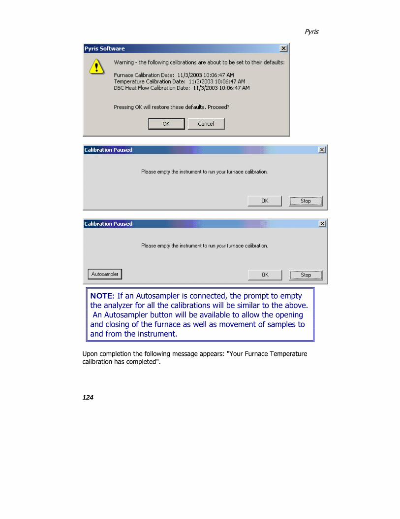
Pyris

124

NOTE: If an Autosampler is connected, the prompt to empty the analyzer for all the calibrations will be similar to the above. An Autosampler button will be available to allow the opening and closing of the furnace as well as movement of samples to and from the instrument.

Upon completion the following message appears: "Your Furnace Temperature calibration has completed".

Calibration

125

NOTE: If you want to perform the Sample Temperature Calibration automatically, continue with step 11. If you want to run it manually, go to step 12.

Click Next to open the Sample Temperature Calibration window.

Using the Add and Edit functions make the appropriate changes.

Pyris

126

After entering the Sample Temperature Calibration, either edit the standard or add new standard and delete the one you do not want. There must be a minimum of two standards.

Selecting Run will run the standards at the rate selected. (This will create a method and run the standards automatically.) See Calibration Reference Materials from Ambient to 725°C and Calibration Reference Materials for Subambient Operation for a list of standards.

-

Several prompts will appear during the sample temperature calibration.

Calibration

127

When the Sample Temperature is completed, select Next to advance the wizard to the Heat Flow Calibration. Continue to step 14.

To calibrate Sample Temperature manually.

NOTE: If you have any Sample Temperature correction that has been applied then you need to restore the Sample Temperature calibration to their default values. Do this by selecting Restored DSC in the Initial Calibration Wizard page before proceeding.

Set up a method to run indium, collect data, calculate the onset and heat flow values. Record these values.

Set up a method to run your other standard(s), collect data, calculate the onset and heat flow values. Record these values.

Open the calibration routine and click Next until the Sample Temperature Calibration Window appears. Edit and Add the appropriate standards and information. Then click Accept, and the Sample Temperature will be calibrated. When the Sample Temperature calibration is completed, select Next to advance the wizard to the next step of the calibration (Heat Flow).

Pyris

128

NOTE: There are 3 ways to perform Heat Flow Calibration. If you calibrated the Sample Temperature automatically within the wizard, see step 13. If you calibrated the Sample Temperature manually, see step 14. Continue with step 15 if you would like to run a new standard for Heat Flow Calibration.

After completing the Sample Temperature calibration, the Heat Flow calibration is performed. A dialog box will appear if you had perform the Sample Temperature calibration wizard automatically. The dialog ask "Do you want to use the area values from the temperature calibration for Heat Flow Calibration?' . If Yes is selected, click the Edit button to display the Add/Edit dialog box. Enter the expected Heat Flow value for each of the listed standards. (The undesired standards may be deleted.) Click on the Accept button to update and save new changes to the calibration.

If you have calibrated the Sample Temperature manually, click on the Add or Edit button to display the Edit dialog. Enter the desired values for all entry fields: Expected, Measured, Temperature, Weight, and Scan Rate. Click on the Accept button to update and save new changes to the calibration.

Following the wizard, the calibration will be performed automatically. Click on the Add or Edit button to display the Edit dialog. Enter the desired values for the Expected Peak Area. Click on the Run button and methods will be created, data collected and calculated automatically.

Calibration

129

Dialog for step 14, 15, and 16.

The finish dialog appears:

Pyris

130

The finish dialog will allow the files used in the calibration to be viewed. These files will only be present if the calibration was performed in the automatic mode. These files include the methods and data file names which were created and used to calibrate the system.

Click Finish. The “Save As” window opens:

Calibration

131

At this window, save the calibration file and the system will be completely calibrated.

Temperature PID Settings

The tree control contains a single root item with the title and the date of most recent recalibration. The proportional, integral and differential values are displayed from the single PID Calibration Date. PID values do not need to be changed. These are fixed for a given analyzer. You may change these if you want, but for our standard calibrations, they should be kept at the default values (PID values may need to be adjusted when Furnace is changed usually done by a Service Engineer).

See Change the PID Values dialog for detailed information.

Click Edit and Accept if there are any changes to the PID.

Default PID Values P I D

Pyris

132

Sapphire DSC 10 500 10

Diamond TG/DTA 10 500 3

Change the PID Values

Proportional

Sapphire DSC Range: 1 ≤ P ≥ 1000 Sapphire DSC Default: 10

Diamond TG/DTA Range: 1 ≤ P ≥ 1000 Diamond TG/DTA Default: 10

The furnace control system produces a correction that is proportional to the difference between the program temperature and the sample temperature. A control equation that uses only proportional control will typically maintain a sample temperature within a close range of the program temperature. It typically does not converge to the program temperature and there is often some constant offset. The higher the proportional gain the greater the response of the furnace control system and it is likely to overshoot the program temperature.

Integral

Sapphire DSC Range: 1 ≤ I ≥ 1000 Sapphire DSC Default: 500

Diamond TG/DTA Range: 10 ≤ I ≥ 1000 Diamond TG/DTA Default: 500

The furnace control system produces a correction based on the integral of the difference between the program temperature and the sample temperature. The area accumulated by the offset, as swept through time, is added to the control instructions until the sample temperature moves toward the program temperature, gradually zeroing out any remaining offset. This term is usually not used in controlling the furnace temperature.

Differential

Calibration

133

Sapphire DSC Range: 1 ≤ D ≥ 1000 Sapphire DSC Default: 10

Diamond TG/DTA Range: 0 ≤ D ≥ 1000 Diamond TG/DTA Default: 3

The furnace control system produces a correction based on the time derivative of the difference between the program temperature and the sample temperature. This control minimizes overshoot and undershoots of the program temperature by controlling the slope of the sample temperature versus time curve. This component of the furnace control typically responses more slowly and can eliminate any constant offset between the sample temperature and the program temperature.

Enters the standard information into the standard list and the dialog box closes.

Causes no changes to the standard list. The calibration store is NOT Marked as changed. The dialog closes.

Sapphire DSC Furnace Calibration

Select this to view the entire Sapphire Calibration Procedure.

Click on the Edit button to make changes to the Furnace Calibration Temperature range and Setpoints.

Pyris

134

Recommended:

To calibrate the Sapphire DSC select Edit and use the values of 50 (Starting), 500 (Ending) and 10 Setpoints. With these values, the analyzer will be calibrated at 50°C, 100C, 150°C, 200°C, 250°C, 300°C, 350°C, 400°C, 450°C, and 500°C.

The setpoints are calculated by the formula below: ∆T = (Max-Min)/N-1

∆T = temperature steps for calibration

N = numbers of setpoints

Max = maximum temperature

Calibration

135

Min = minimum temperature

A message box will display if you try to perform the calibration using the default values after selecting the Edit button. A method will automatically be generated to perform the calibration based on the Starting Temperature, Ending Temperature, and Number of Setpoints.



Pyris

136


Upon completion the following message appears: "Your Furnace Temperature calibration has completed". Select OK to close the message window. Select Next until the"Save As" window appears. Save the calibration.

Change the Furnace Calibration

Starting Temperature

Enter a value for the Starting Temperature.

Sapphire DSC Range: -200.0 °C to 750.0 °C. Sapphire DSC Default: 50

Diamond TG/DTA Range: 0.0°C to 1550.0 °C. Diamond TG/DTA Default: 100

Ending Temperature

Enter a value for the Ending Temperature.

Calibration

137



Number of Setpoints

Enter a value to change the number of setpoints to be used over the specified range.

Sapphire DSC Range: 4 to 10 Sapphire DSC Default: 10

Diamond TG/DTA Range: of 4 to 20. Diamond TG/DTA Default: 6



Sapphire DSC Temperature Calibration

Select this to view the entire Sapphire DSC Calibration Procedure.

In the Sample Temperature Calibration window, use the Add and Edit functions make the appropriate changes.

Pyris

138

Calibration

139


Selecting Run will run the standards at the rate selected. (This will create a method and run the standards automatically.) See Calibration Standards for the Sapphire DSC for a list of standards.

-


Pyris

140

When the Sample Temperature is completed, select Next to advance the wizard to the Heat Flow Calibration.


NOTE: If you have any Sample Temperature correction that has been applied then you need to restore the Sample Temperature calibration to their default values. Do this by selecting Restored DSC in the Initial Calibration Wizard page before proceeding.

Set up a method to run indium, collect data, calculate the onset and heat flow values. Record these values.

Set up a method to run your other standard(s), collect data, calculate the onset and heat flow values. Record these values.


Add/Edit a Temperature Standard

Standard Name

Enter a standard name in the edit field box. There is an unlimited number of characters allowed. A duplicate name is not allowed. The names must be unique to this calibration. Spaces and special characters are allowed.

Temperature, Expected

Enter a value for the melting point of the standard within the allowed range in the Expected edit field box. The values are sorted into the list of standards based on its values.

Sapphire DSC Range: -200.0°C to 750.0°C. Sapphire DSC Default: 100

Calibration

141

Diamond TG/DTA Range: 0.0°C to 1550.0°C Diamond TG/DTA Default: 100

Temperature, Measured

Enter a measured (experimental) value for the melting point of the standard within the allowed range in the Measured edit field box. The value is determined by taking the extrapolated onset of the probe position curve at the point in time where the penetration of the probe into the sample first occurs (i.e. the event onset).

Sapphire DSC Range: -200.0°C to 750.0°C. Sapphire DSC Default: 100°C

Diamond TG/DTA Range: 0.0°C to 1550.0°C Diamond TG/DTA Default: 100°C

Scan Rate

Enter a value in the Scan Rate edit field box within the allowed range, this rate will be used as a scan rate for an instrument run when the user clicks on the Run Standard button on the Sample Temperature Standard dialog.

Sapphire DSC Range: 0.01°C/min to 200.0 °C/min Sapphire DSC Default: 10 °C/min

Diamond TG/DTA Range: 0.01 to 9999.0 °C/min Diamond TG/DTA Default: 10 °C/min

Sample Weight

Enter a value in the Sample Weight edit field box within the allowed range, this value will be used as a sample weight for an instrument run when the user clicks on the Run Standard button on the Sample Temperature Standard dialog.

Sapphire DSC Range: 0.01mg to 1000.0 mg Sapphire DSC Default: 1mg

Diamond TG/DTA Range: 0.01mg to 1000.0 mg Diamond TG/DTA Default: 1mg

Pyris

142



There are 2 case scenarios:

The dialog was accessed from Add Standard – the standard is added to the standard list. The standard is placed into the list in increasing numeric order sorted by Expected Temperature. The range of values for the Regression Order is adjusted accordingly (see the Edit Equation dialog). The calibration store is marked as changed.

The dialog was accessed from Edit Standard – the standard in the list is changed to reflect the new values. If the Expected Temperature changed the list is resorted in increasing numeric order on the Expected Temperature. The calibration store is marked as changed.

Sapphire DSC Heat Flow Calibration


The tree control contains roots for all of the calibrations with their names and dates. Each Heat Flow standard will have a branch with the standard name. Each standard will have the following information under it as a leaf:

Expected Temperature (literature value) Melting Point °C

Expected (literature value) Heat of Fusion (J/g)

Measured (experimentally determined) Heat of Fusion (J/g)

Sample Weight (mg)

Correction Order and Polynomial for the correction are displayed as separate branches.

Calibration

143

NOTE: There are 3 ways to perform Heat Flow Calibration. Choose the appropriate procedure below If you calibrated the Sample Temperature automatically within the wizard, if you calibrated the Sample Temperature manually, or if you would like to run a new standard for Heat Flow Calibration.

Calibrated the Sample Temperature automatically within the wizard

After completing the Sample Temperature calibration, the Heat Flow calibration is performed. A dialog box will appear if you had perform the Sample Temperature calibration wizard automatically. The dialog ask ' Do you want to use the area values from the temperature calibration for Heat Flow Calibration?' . If Yes is selected, click the Edit button to display the Add/Edit dialog box. Enter the expected Heat Flow value for each of the listed standards. (The undesired standards may be deleted.) Click on the Accept button to update and save new changes to the calibration.

Calibrated the Sample Temperature Manually


Run a new standard for Heat Calibration


Pyris

144

Add Edit a Sapphire DSC Heat Flow Standard

Standard Name

Enter the name of the standard in the Standard Name field box. Any number of characters is allowed. A name that matches any of the other specified standard names is not allowed (they must be unique to this calibration). Spaces and special characters are allowed.

Calibration

145

Peak Area, Expected

Enter a literature value within the ranges of 0.001 to 10000.0 in the Expected Peak Area field box.

Peak Area, Measured

Enter a measured value within the ranges of 0.001 to 10000.0 in the Measured Peak Area field box. The value is determined by taking the peak area of the heat flow curve at the melting peak.

Temperature

Enter the expected melting point value within the ranges of -200.0°C to 750.0°C in the Temperature field box. The standards will be sorted based on this value. This value will also be used to build a temperature program for Run Standards.

Scan Rate

Enter the value for the Scan Rate within the ranges of 0.01°C/min to 200°C/min in the San Rate field box. This scan rate will be used as the scan rate for an instrument run when Run Standards is selected.

Weight

Enter the value for Weight within the ranges of 0.01mg to 1000.0mg in the Weight field box. This weight will be used for the peak area calculation when Run Standards is used.

Enters the standard information into the standard list and the dialog closes. The action taken falls into one of two cases:

The dialog was accessed from Add Standard – the standard is added to the standard list. The standard is placed into the list in increasing numeric order

Pyris

146

sorted by Temperature. The range of values for the Regression Order is adjusted accordingly (see the Edit Equation dialog). The calibration store is marked as changed.

The dialog was accessed from Edit Standard – the standard in the list is changed to reflect the new values. If the Temperature changed the list is resorted in increasing numeric order on the Temperature. The calibration store is marked as changed.

Causes no changes to the standard list. The calibration store is NOT marked as changed.

Calibration Finished

Tree Control View: Right-clicking in the tree control view area causes a drop-down menu to appear with selections of Expand All and Collapse All. The user may also click on the plus icon at the root to expand or click on the minus icon at the root to collapse. The displayed calibrations are listed in their calibration order. There is a scrollable test view showing a list of all files generated in this session. Select the links below for Diamond Instruments Calibration Finished.

Sapphire DSC Calibration Finished

Diamond TG/DTA Calibration Finished

Diamond TMA Calibration Finished

Sapphire DSC Finished Calibration

The Sapphire DSC Summary dialog appears: See Generated Calibration Files Dialog. The Summary dialog will allow the files used in the calibration to be viewed. These files will only be present if the calibration was performed in the automatic mode. These files include the methods and data file names which were created and used to calibrate the system.

Calibration

147

Click Finish. The "Save As" Window appears. At this window, save the calibration file and the system will be completely calibrated.

Pyris

148

Diamond TMA Calibration

Diamond TMA Calibration Procedure

From Pyris Manager open the Instrument Application.

Upon opening the Instrument Application, you will be prompted to perform the probe initialization. Calibrating the Diamond TMA requires the probe to be initialized before calibration can begin. If you have not done this, the probe can

be initialized from the control panel using the probe initialization icon . In order to perform the initialization procedure, the measuring system of your analysis should be installed and the instrument should be without any samples. The initialization process needs to be perform each time the measuring system is changed. The probe weight is displayed at the bottom of the Pyris Window after the initialization of the probe. The initialize probe message box appears:

After initializing the probe, with the “Method Editor” window open, from the menu bar, select View\Calibrate. The initial Calibration Wizard screen appears:

Calibration

149

3.1 Calibration Wizard:




Force PID values do not need to be changed. These are fixed for a given analyzer. A customer could change these if they want, but for our standard calibrations, they should be kept at the default values.

Pyris

150

Height Calibration, calibrates the displacement transducer that is used to measure the position axis of the Diamond TMA.

Force Calibration, calibrates the force motor that is used to apply the static force to the sample.

Compliance Calibration, corrects for the very small movement of the measuring system itself when large forces are applied.

Load Linearization Calibration, this correction process eliminates the load dependency errors that occurs during the load control by calibrating the force motor. Clicking Begin starts the wizard. The calibration must be made in the order as it is displayed.

The Check the Instrument Environment appears. At this time the gases and cooling accessories should be checked. The current calibrations can be viewed by expanding the list when clicking on the [+] sign or right clicking for Expand All.

Calibration

151

NOTE: The Measuring System/Geometry should be selected in the Method Editor.

Click Next to continue. The Temperature PID Settings appear: PID values do not need to be changed. These are fixed for a given analyzer. You may change these if you want, but for our standard calibrations, they should be kept at the default values.

Pyris

152

The PID are fixed for a specific TMA furnace type (TMA Standard or TMA High Temperature) and should not be changed by users.(PID values may need to be adjusted when Furnace is changed usually done by a Service Engineer). See Change the Diamond TMA PID Values dialog for detailed information.

5.1 Click Edit and Accept if there are any changes to the PID (PID values may need to be adjusted when Furnace is changed usually done by a Service Engineer).

By Default P I D

Calibration

153

Standard Furnace 50 500 3

High temperature Furnace

10 500 3

Click Next. The Diamond Furnace Calibration appears: Furnace calibration functions as the “Precalibration” mode of the Exstar/Muse Software. It will calibrate the Sensor Temperature to the Program Temperature. When the instrument is initially installed, the calibration will take on its default values.

Pyris

154

6.1 Click Edit to make changes to the Furnace Calibration Temperature range and Setpoints. See Change the Diamond TMA Furnace Calibration dialog a list of allowed ranges.

Recommended: To calibrate the Diamond TMA (low temperature), select Edit and use the values of 100°C (Starting), 600°C (Ending) and 11 Setpoints. With Start and End Temperatures selected with 11 setpoints, the Furnace Calibration window will be updated with the newly calculated values. To calibrate the Diamond TMA (high temperature), select Edit and use the values of 100°C (Starting), 1500°C (Ending) and 14 Setpoints. With Start and End Temperatures selected with 14 setpoints, the Furnace Calibration window will be updated with the newly calculated values.

Calibration

155






6.2 A message box will display if you try to perform the calibration using the default values after selecting the Edit button. A method will automatically be generated to perform the calibration based on the Starting Temperature, Ending Temperature, and Number of Setpoints.

6.3 After selection of the limits, select Run.

Pyris

156


Calibration

157

Click on Sample Load, Sample Load Procedure, to move the Cylinder when loading or unloading a sample.


Click Next to open the Sample Temperature Calibration window. After entering the Sample Temperature Calibration, either edit the standard or add new standard or delete the one you do not want. There must be a minimum of two standards.

Pyris

158

Use the Add and Edit functions to make the appropriate changes. See Edit dialog for a list of ranges.

Calibration

159

If you determined the melting temperature of your standard material outside the Calibration Wizard, then you will use the Edit function to manually enter the Measured Temperature followed by the Accept button to start the calibration.

Selecting Run will run the standards at the rate selected. (This will create a method and run the standards automatically.) See Calibration Standards for the Diamond TMA for a list of standards. Several prompts will appear during the sample temperature calibration.

Pyris

160

When the Sample Temperature is completed, select Next to advance the wizard to the Force PID Calibration.

The Diamond TMA Force PID Settings dialog appears: Force PID values do not need to be changed. These are fixed for a given analyzer. You may change these if you want, but for our standard calibrations, they should be kept at the default values. The current calibrations can be viewed when clicking on the [+]. PIDs for Force are fixed for a TMA furnace type (TMA Standard or TMA High Temperature) and should not be changed by users. See Change the Diamond TMA Force PID Values dialog for detailed information so that you can change values for Proportional, Integral, and Differential.

Calibration

161

By Default P I D



1 30 3

Pyris

162

Select Next to advance the wizard to the Height Calibration.

The Diamond TMA Force Calibration dialog appears: Force Calibration, calibrates the force motor that is used to apply the static force to the sample.

Note: During force calibration, do not click on the Sample Load button. Clicking on the Sample Load button, during force calibration, will result in a failure of the force calibration.

Selecting Run will start the Force Calibration procedure. This calibrates the force motor that is used to apply the static force to the sample. Several prompts will appear during the Force procedure.

Calibration

163

NOTE: This procedure may take up to 3 minutes.

Pyris

164

Calibration

165

Pyris

166

Calibration

167

Pyris

168

Select Next to advance the wizard to the Compliance Calibration.

Calibration

169

The Diamond TMA Height dialog appears: Selecting Run will start the Height calibration. Several prompts will appear during the Height calibration. See Sample Load Procedure for Extension.

Pyris

170

Select Next to advance the wizard to the Force Calibration.

Calibration

171

The Diamond TMA Compliance Settings dialog appear: Starts the compliance calibration. This corrects the very small movement of the measuring system itself when large forces are applied. The Edit button displays the Change the Final Force dialog. Selecting Run will start the Compliance procedure. This corrects the very small movement of the measuring system itself when large forces are applied. A prompt will appear during the Compliance procedure.

Pyris

172

NOTE: Default values are from 100 mN to 500 mN. This calibration takes 10 minutes. The required time for the Compliance calibration is determined by the second force. This scans for additional one minute (50mN/minute) for the First Force Setpoint and Second Force Setpoint. For example see sample 1.

Calibration

173

NOTE: Increasing the Maximum Force will increase the time required to complete this calibration.

Pyris

174

Select Next to advance the wizard to the Load Linearization Calibration.

The Diamond TMA Load Linearization Settings dialog appears: Load Linearization Calibration, this correction process eliminates the load dependency errors that occurs during the load control by calibrating the force motor. Selecting Run starts the Load Linearization calibration. Load Linearization Calibration, this correction process eliminates the load dependency errors that occurs during the load control by calibrating the force motor.

Calibration

175


NOTE: Load Linearization is never restored. It is only restored if the batteries have been changed or the CPU board has been replaced.

Several prompts will appear during the Load Linearization Calibration.

Pyris

176

Select Next to advance the wizard to the Summary Calibration.

The Diamond TMA Summary dialog appears: The Summary dialog will allow the files used in the calibration to be viewed. These files will only be present if the calibration was performed in the automatic

Calibration

177

mode. These files include the methods and data file names which were created and used to calibrate the system.


Pyris

178

Introduction to the Calibration of the Diamond and Sapphire Instruments

The Sapphire DSC, Diamond TMA, and Diamond TG/DTA is calibrated when it is first installed by a PerkinElmer Service Engineer. The analyzer remains calibrated, even when the system is turned off, as long as there are no major changes to operating conditions (such as a change or switching to a different purge gas rate). As part of maintaining proper operating conditions for your instrument, it is recommended also that the DSC, TMA, and TG/DTA be calibrated every three to six months after installation or whenever you change the furnace, balance beams, or experimental conditions. Select the link below for the appropriate Diamond Instruments introduction.

Although instrument calibration will remain steady for several months over a given calibration range, it is advisable to check the calibration more frequently as part of your standard operating procedure. This can be done by setting up a Pyris Player to run your calibrants as samples. The data produced can be analyzed within Player using a tolerance test to confirm that the current calibration is still valid. An example of such a player is included on the install disk.

Sapphire DSC Calibration Introduction

Diamond TMA Calibration Introduction

Diamond TG/DTA Calibration Introduction

Diamond TMA Environment

Select this to view the entire Diamond TMA Calibration Procedures.

The Check the Instrument Environment appears. At this time the gases and cooling accessories should be checked. The current calibrations can be viewed by expanding the list when clicking on the [+] sign or right clicking for Expand All.

Calibration

179

NOTE: The Measuring System/Geometry should be selected in the Method Editor.

Diamond TMA Temperature PID Settings Select this to view the entire Diamond TMA Calibration Procedures.

Pyris

180

PID values do not need to be changed. These are fixed for a given analyzer. You may change these if you want, but for our standard calibrations, they should be kept at the default values.

The PID are fixed for a specific TMA furnace type (TMA Standard or TMA High Temperature) and should not be changed by users.(PID values may need to be adjusted when Furnace is changed usually done by a Service Engineer). See Change the Diamond TMA PID Values dialog for detailed information.

The Diamond Temperature PID Settings appear:

Click Edit and Accept if there are any changes to the PID

Calibration

181

By Default P I D



10 500 3

Diamond TMA Furnace Calibration Select this to view the entire Diamond TMA Calibration Procedures.


Furnace calibration functions as the “Precalibration” mode of the Exstar/Muse Software. It will calibrate the Sensor Temperature to the Program Temperature. When the instrument is initially installed, the calibration will take on its default values.

Click Edit to make changes to the Furnace Calibration Temperature range and Setpoints. See Change the Diamond TMA Furnace Calibration dialog a list of allowed ranges.

Pyris

182

Recommended: To calibrate the Diamond TMA (low temperature), select Edit and use the values of 100°C (Starting), 600°C (Ending) and 11 Setpoints. With Start and End Temperatures selected with 11 setpoints, the Furnace Calibration window will be updated with the newly calculated values. To calibrate the Diamond TMA (high temperature), select Edit and use the values of 100°C (Starting), 1500°C (Ending) and 14 Setpoints. With Start and End Temperatures selected with 14 setpoints, the Furnace Calibration window will be updated with the newly calculated values. The setpoints are calculated by the formula below:

Calibration

183

∆T = (Max-Min)/N-1







Pyris

184


Calibration

185

Click on Sample Load, Sample Load Procedure, to move the Cylinder when loading or unloading a sample.


Change the Diamond TMA Furnace Calibration


Enter a value in the Starting Temperature edit field box.

Standard: -200.0°C to 650.0 °C Standard Default: 50 °C

Pyris

186

Hi-Temp: 0.0°C to 1550.0 °C Hi-Temp Default: 100 °C

Ending Temperature

Enter a value in the Ending Temperature edit field box.

Standard: -200.0°C to 650.0 °C Standard Default: 500 °C

Hi-Temp: 0.0°C to 1550.0 °C Hi-Temp Default: 1000.0 °C

Number of Setpoints

Enter a value in the Number of Setpoints edit field box.

Standard: 4 to 20 Standard Default: 10

Hi-Temp: 4 to 20 Hi-Temp Default: 10



Diamond TMA Sample Temperature Calibration



Calibration

187

The Sample Temperature Calibration window. After entering the Sample Temperature Calibration, either edit the standard or add new standard or delete the one you do not want. There must be a minimum of two standards.

Use the Add and Edit functions to make the appropriate changes. See Edit dialog for a list of ranges.

Pyris

188

If you determined the melting temperature of your standard material outside the Calibration Wizard, then you will use the Edit function to manually enter the Measured Temperature followed by the Accept button to start the calibration.

Selecting Run will run the standards at the rate selected. (This will create a method and run the standards automatically.) See Calibration Standards for the Diamond TMA for a list of standards. Several prompts will appear during the sample temperature calibration.

Calibration

189

When the Sample Temperature is completed, select Next to advance the wizard to the Force PID Calibration.

Diamond TMA Force PID Settings


Force PID values do not need to be changed. These are fixed for a given analyzer. You may change these if you want, but for our standard calibrations, they should be kept at the default values.

The Diamond TMA Force PID Settings dialog appears: The current calibrations can be viewed when clicking on the [+]. PIDs for Force are fixed for a TMA furnace type (TMA Standard or TMA High Temperature) and should not be changed by users. See Change the Diamond TMA Force PID Values dialog for detailed information so that you can change values for Proportional, Integral, and Differential.

Pyris

190

Calibration

191

By Default P I D



1 30 3

Select Next to advance the wizard to the Height Calibration.

Change the Diamond TMA Force PID Values

Proportional

Standard Range: 1 ≤ P ≤ 1.0e20 Standard Default: 1

Hi-Temp: 1 ≤ P ≤ 1.0e20 HI-Temp Default: 1

The furnace control system produces a correction that is proportional to the difference between the program temperature and the sample temperature. A control equation that uses only proportional control will typically maintain a sample temperature within a close range of the program temperature. It typically

Pyris

192

does not converge to the program temperature and there is often some constant offset. The higher the proportional gain the greater the response of the furnace control system and it is likely to overshoot the program temperature.

Integral


Hi-Temp: 0.001 ≤ P ≤ 1.0e20 HI-Temp Default: 30


Differential


Hi-Temp: 1 ≤ P ≤ 1.0e20 HI-Temp Default: 3



Calibration

193


Diamond TMA Force Calibration


Force Calibration, calibrates the force motor that is used to apply the static force to the sample.

The Diamond TMA Force Calibration dialog appear: Selecting Run will start the Force Calibration procedure. This calibrates the force motor that is used to apply the static force to the sample. Several prompts will appear during the Force procedure.

Pyris

194


Calibration

195

Pyris

196

Calibration

197

Pyris

198

Calibration

199

Select Next to advance the wizard to the Compliance Calibration.

Pyris

200

Diamond TMA Height Calibration


Height Calibration, calibrates the displacement transducer that is used to measure the position axis of the Diamond TMA.

The Diamond TMA Height dialog appears: Selecting Run will start the Height calibration. Several prompts will appear during the Height calibration. See Sample Load for Extension.

Calibration

201

Select Next to advance the wizard to the Force Calibration.

Pyris

202

Diamond TMA Compliance Settings


Starts the compliance calibration. This corrects the very small movement of the measuring system itself when large forces are applied.

NOTE: Default values are from 100 mN to 500 mN. This calibration takes 10 minutes. The required time for the Compliance calibration is determined by the second force. This scans for additional one minute (50mN/minute)

Calibration

203

for the First Force Setpoint and Second Force Setpoint. For example see sample 1.

NOTE: Increasing the Maximum Force will increase the time required to complete this calibration.

The Diamond TMA Compliance Settings dialog appear: The Edit button displays the Change the Final Force dialog. Selecting Run will start the Compliance procedure. This corrects the very small movement of the measuring system itself when large forces are applied. A prompt will appear during the Compliance procedure.

Pyris

204

Calibration

205

Pyris

206

Select Next to advance the wizard to the Load Linearization Calibration.

Diamond TMA Load Linearization Settings


Load Linearization Calibration, this correction process eliminates the load dependency errors that occurs during the load control by calibrating the force motor.

The Diamond TMA Load Linearization Settings dialog appears: Selecting Run starts the Load Linearization calibration. Load Linearization Calibration, this correction process eliminates the load dependency errors that occurs during the load control by calibrating the force motor.

Calibration

207


NOTE: Load Linearization is never restored. It is only restored if the batteries have been changed or the CPU board has been replaced.

Several prompts will appear during the Load Linearization Calibration.

Pyris

208

Select Next to advance the wizard to the Summary Calibration.

Calibration

209







The Diamond TMA Summary dialog appears: See Generated Calibration Files Dialog. The Summary dialog will allow the files used in the calibration to be viewed. These files will only be present if the calibration was performed in the automatic mode. These files include the methods and data file names which were created and used to calibrate the system.

Pyris

210


Calibration

211

Calibration Standards for Diamond TMA

Thermal Capacities of Reference Materials

Reference Material Melting Point (°C)

Indium

156.6

Tin

231.88

Lead 327.47

Zinc

419.51

Aluminum 660.10

Silver

960.85

Nickel

1452.85

Palladium

1551.85

Gold

1063.00

Pyris

212

Calibration

213

Diamond TG/DTA Calibration

Diamond TG/DTA Calibration Procedure

From Pyris Manager Open the instrument application Instrument Application

With the “Method Editor” window open, from the menu bar, select View\Calibrate. The initial Calibration Wizard screen appears:

Clicking Begin starts the wizard. The calibration must be made in the exact order as it is displayed.

Pyris

214




DTA Heat Flow Calibration, calibrates the heat flow, ∆H value calculated to a reference material

DTA Slope Calibration, corrects the slope of the DTA curve by aligning two preselected points on the DTA curve.

TGA Weight Calibration, calibrates the weighing component of the TG/DTA. This is typically done with a known weight (i.e. 20 mg) at room temperature. It can also be done at selected points at elevated temperatures.

Click Next. The Check the Instrument Environment appears:

Calibration

215

Click Next to continue. The Diamond Temperature PID Settings appear:

Pyris

216

Click Edit or Accept to make changes to the PID.

Click Next. The Diamond Furnace Calibration appears:

Calibration

217

Click Edit to make changes to the Furnace Calibration.

Pyris

218

Furnace calibration functions as the “Precalibration” mode of the Exstar/Muse Software. It will match the “Program” and “Sample” Temperatures. A method will automatically be generated to perform the calibration based on the Starting Temperature, Ending Temperature, and Number of Setpoints.

To calibrate the Diamond TG/DTA, select Edit and use the values of 100 (Starting), 1500 (Ending) and 8 Setpoints. With these values, the analyzer will be calibrated at 100°, 300°, 500°, 700°, 900°, 1100°, 1300°, and 1500°C.


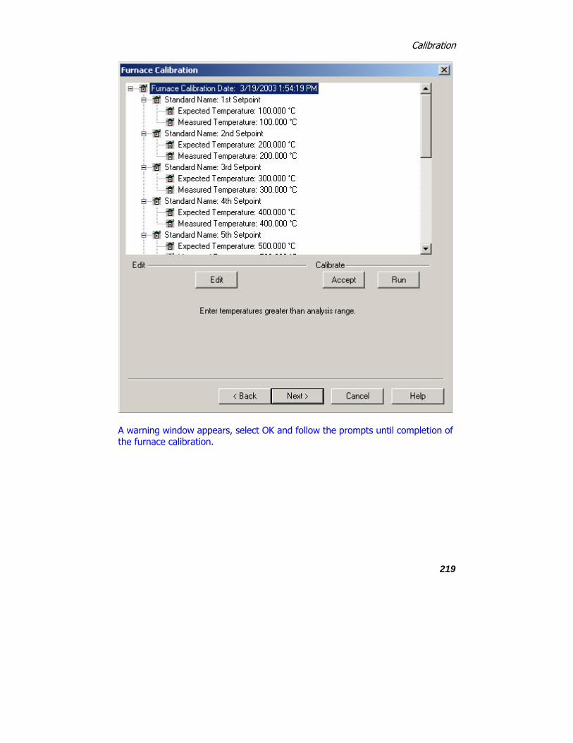
Calibration

219


Pyris

220



Calibration

221

Select OK to close the message window. Select Next until the"Save As" window appears. Save the calibration.

NOTE: If you want to perform the Sample Temperature Calibration automatically (recommended) , continue with step 12. If you want to run it manually, go to step 13.

Re-enter the calibration and click Next to open the Sample Temperature Calibration window.

Pyris

222

Using the Add and Edit functions make the appropriate changes.


Selecting Run will run the standards at the rate selected. (This will create a method and run the standards automatically.) See Calibration Standards for the Diamond TG/DTA for a list of standards.

Calibration

223

-


Pyris

224

When the Sample Temperature is completed, select Next to advance the wizard to the Heat Flow Calibration. Continue to step 14.


After Furnace Calibration, close the calibration window.

Set up a method to run indium, collect data, calculate the onset and heat flow values (heat flow should be calculated on the DTA curve (uV.s). Record these values.

Set up a method to run your other standard(s), collect data, calculate the onset and heat flow values (heat flow should be calculated on the DTA curve (uV.s). Record these values.


NOTE: There are 3 ways to perform Heat Flow Calibration. If you calibrated the Sample Temperature automatically within the wizard, see step 14. If you calibrated the Sample Temperature manually, see step 15. Continue with step 16 if you would like to run a new standard for Heat Flow Calibration.

After completing the Sample Temperature calibration, the Heat Flow calibration is performed. A dialog box will appear if you had perform the Sample Temperature calibration wizard automatically. The dialog ask ' Do you want to

Calibration

225

use the area values from the temperature calibration for Heat Flow Calibration?' . If Yes is selected, click the Edit button to display the Add/Edit dialog box. Enter the expected Heat Flow value for each of the listed standards. (The undesired standards may be deleted.) Click on the Accept button to update and save new changes to the calibration.



Pyris

226

Dialog for step 14, 15, and 16.

TG/DTA Slope Calibration will correct for the slope in the DTA signal curve.

Calibration

227

This is done at two points identified by the user. The first point should be no less than 100 °C, the second 50° to 100°C below the maximum temperature used in the furnace calibration. A respective scan rate should be used.

The following screen appears. Click OK.

Pyris

228

Weight calibration is the final step in the calibration process. Normal service verification calls for the weight calibration to be checked at room temperature (Single Point Calibration). This is accomplished using the 20 mg weight supplied with the analyzer. If the weight calibration is to be performed at room temperature, click on the Weigh button and follow the instructions.

Calibration

229

If the calibration is to be done at multiple temperatures, input the starting and end temperatures as well as the weight (see note below). Input the expected weight of the reference weight. Click Run to perform the calibration per the starting and ending temperature limits.

Pyris

230

NOTE: Do Not use the aluminum weight supplied with the analyzer if the weight calibration is performed at temperatures (Multi-Point Calibration). To perform this type of weight calibration use a platinum pan whose weight has been predetermined using an analytical microbalance.

A warning prompt appears indicating the weight calibration will proceed. Click OK.

Calibration

231

After the weight calibration is completed, click OK.

Pyris

232

The finish dialog appears:

Calibration

233

The finish dialog will allow the files used in the calibration to be viewed. These files will only be present if the calibration was performed in the automatic mode. These files include the methods and data file names which were created and used to calibrate the system.

Click Finish. The “Save As” window opens:

Pyris

234

At this window, save the calibration file and the system will be completely calibrated.

Introduction to the Calibration of the Diamond and Sapphire Instruments

The Sapphire DSC, Diamond TMA, and Diamond TG/DTA is calibrated when it is first installed by a PerkinElmer Service Engineer. The analyzer remains calibrated, even when the system is turned off, as long as there are no major changes to operating conditions (such as a change or switching to a different purge gas rate). As part of maintaining proper operating conditions for your instrument, it is recommended also that the DSC, TMA, and TG/DTA be calibrated every three to six months after installation or whenever you change the furnace, balance beams, or experimental conditions. Select the link below for the appropriate Diamond Instruments introduction.

Although instrument calibration will remain steady for several months over a given calibration range, it is advisable to check the calibration more frequently as part of your standard operating procedure. This can be done by setting up a

Calibration

235

Pyris Player to run your calibrants as samples. The data produced can be analyzed within Player using a tolerance test to confirm that the current calibration is still valid. An example of such a player is included on the install disk.

Sapphire DSC Calibration Introduction

Diamond TMA Calibration Introduction

Diamond TG/DTA Calibration Introduction

Diamond TG/DTA Enviroment Select this to view the entire Diamond TG/DTA Calibration Procedures.

This dialog displays the roots for all of the calibrations with their names and dates. Calibration roots are:

Temperature PID

Sample Temperature

Furnace Temperature

DTA Heat Flow

DTA Slope

TGA Weight

The branches and leaves are specified for each root calibration.

Displays the previous page which is the initial calibration page.

Pyris

236

Displays the proceeding page which is the Temperature PID page.

Stops the calibration procedure.

Displays the Pyris help for this page.

Temperature PID Settings

The tree control contains a single root item with the title and the date of most recent recalibration. The proportional, integral and differential values are displayed from the single PID Calibration Date. PID values do not need to be changed. These are fixed for a given analyzer. You may change these if you want, but for our standard calibrations, they should be kept at the default values (PID values may need to be adjusted when Furnace is changed usually done by a Service Engineer).

See Change the PID Values dialog for detailed information.

Click Edit and Accept if there are any changes to the PID.

Default PID Values P I D

Sapphire DSC 10 500 10

Diamond TG/DTA 10 500 3

Calibration

237

Change the PID Values

Proportional

Sapphire DSC Range: 1 ≤ P ≥ 1000 Sapphire DSC Default: 10

Diamond TG/DTA Range: 1 ≤ P ≥ 1000 Diamond TG/DTA Default: 10

The furnace control system produces a correction that is proportional to the difference between the program temperature and the sample temperature. A control equation that uses only proportional control will typically maintain a sample temperature within a close range of the program temperature. It typically does not converge to the program temperature and there is often some constant offset. The higher the proportional gain the greater the response of the furnace control system and it is likely to overshoot the program temperature.

Integral

Sapphire DSC Range: 1 ≤ I ≥ 1000 Sapphire DSC Default: 500

Diamond TG/DTA Range: 10 ≤ I ≥ 1000 Diamond TG/DTA Default: 500


Differential

Sapphire DSC Range: 1 ≤ D ≥ 1000 Sapphire DSC Default: 10

Pyris

238

Diamond TG/DTA Range: 0 ≤ D ≥ 1000 Diamond TG/DTA Default: 3




Furnace Calibration


Furnace calibration functions as the “Precalibration” mode of the Exstar/Muse Software. It will calibrate the Sensor Temperature to the Program Temperature. When the instrument is initially installed, the calibration will take on its default values.

Select on the link below for the appropriate instrument.

Sapphire DSC

Diamond TG/DTA

Calibration

239

Sapphire DSC Furnace Calibration



Recommended:

To calibrate the Sapphire DSC select Edit and use the values of 50 (Starting), 500 (Ending) and 10 Setpoints. With these values, the analyzer will be calibrated at 50°, 100°, 150°, 200°, 250°, 300°, 350°, 400°, 450°, and 500°.

Pyris

240









Calibration

241



Diamond TG/DTA Furnace Calibration Select this to view the entire Diamond TG/DTA Calibration Procedures.


Pyris

242

Recommended:

To calibrate the Diamond TG/DTA, select Edit and use the values of 100 (Starting), 1500 (Ending) and 8 Setpoints. With these values, the analyzer will be calibrated at 100°, 300°, 500°, 700°, 900°, 1100°, 1300°, and 1500°C.









Calibration

243


Pyris

244


Change the Furnace Calibration


Enter a value for the Starting Temperature.



Ending Temperature

Enter a value for the Ending Temperature.



Number of Setpoints

Enter a value to change the number of setpoints to be used over the specified range.

Sapphire DSC Range: 4 to 10 Sapphire DSC Default: 10

Diamond TG/DTA Range: of 4 to 20. Diamond TG/DTA Default: 6

Calibration

245



Temperature Calibration

The tree control contains roots for all of the calibrations with their names and dates. Each temperature standard will have a branch with the standard name. Each temperature standard will have the following information under it:

Expected Temperature

Measured Temperature

Sample Weight

Preferred Scan Rate

The correction order and the polynomial for the correction are displayed as separate branches.

When you right click in the tree control view area. A drop down menu appears with selections of Expand All, Collapse All, and Edit Values. You may also click on the plus icon at the root to expand or click on the minus icon at the root to collapse. Expanding the root will display: Expected Temperature, Measured Temperature, Sample Weight, and Preferred Scan Rate.

Sapphire DSC

Diamond TG/DTA

Pyris

246

Sapphire DSC Temperature Calibration


Calibration

247


Selecting Run will run the standards at the rate selected. (This will create a method and run the standards automatically.) See Calibration Standards for the Sapphire DSC for a list of standards.

-


Pyris

248







Calibration

249

Diamond TG/DTA Temperature Calibration


Pyris

250


Selecting Run will run the standards at the rate selected. (This will create a method and run the standards automatically.) See Calibration Standards for the Diamond TG/DTA for a list of standards.

Calibration

251

-


Pyris

252


To calibrate Sample Temperature manually





Add/Edit a Temperature Standard

Standard Name

Enter a standard name in the edit field box. There is an unlimited number of characters allowed. A duplicate name is not allowed. The names must be unique to this calibration. Spaces and special characters are allowed.

Temperature, Expected

Calibration

253

Enter a value for the melting point of the standard within the allowed range in the Expected edit field box. The values are sorted into the list of standards based on its values.

Sapphire DSC Range: -200.0°C to 750.0°C. Sapphire DSC Default: 100

Diamond TG/DTA Range: 0.0°C to 1550.0°C Diamond TG/DTA Default: 100

Temperature, Measured

Enter a measured (experimental) value for the melting point of the standard within the allowed range in the Measured edit field box. The value is determined by taking the extrapolated onset of the probe position curve at the point in time where the penetration of the probe into the sample first occurs (i.e. the event onset).

Sapphire DSC Range: -200.0°C to 750.0°C. Sapphire DSC Default: 100°C

Diamond TG/DTA Range: 0.0°C to 1550.0°C Diamond TG/DTA Default: 100°C

Scan Rate

Enter a value in the Scan Rate edit field box within the allowed range, this rate will be used as a scan rate for an instrument run when the user clicks on the Run Standard button on the Sample Temperature Standard dialog.

Sapphire DSC Range: 0.01°C/min to 200.0 °C/min Sapphire DSC Default: 10 °C/min

Diamond TG/DTA Range: 0.01 to 9999.0 °C/min Diamond TG/DTA Default: 10 °C/min

Sample Weight

Enter a value in the Sample Weight edit field box within the allowed range, this value will be used as a sample weight for an instrument run when the user clicks on the Run Standard button on the Sample Temperature Standard dialog.

Pyris

254

Sapphire DSC Range: 0.01mg to 1000.0 mg Sapphire DSC Default: 1mg

Diamond TG/DTA Range: 0.01mg to 1000.0 mg Diamond TG/DTA Default: 1mg



There are 2 case scenarios:

The dialog was accessed from Add Standard – the standard is added to the standard list. The standard is placed into the list in increasing numeric order sorted by Expected Temperature. The range of values for the Regression Order is adjusted accordingly (see the Edit Equation dialog). The calibration store is marked as changed.

The dialog was accessed from Edit Standard – the standard in the list is changed to reflect the new values. If the Expected Temperature changed the list is resorted in increasing numeric order on the Expected Temperature. The calibration store is marked as changed.

Diamond TG/DTA Heat Flow Calibration

Select this to view the entire Diamond TG/DTA Calibration Procedures.

The tree control contains roots for all of the calibrations with their names and dates. Each DTA standard displays a branch with the standard name and will have the following information under it:

Expected Temperature (literature value) Heat Flow (mW)

Calibration

255

Measured Temperature (experimentally determined) Heat Flow (uV.s/mg)

Expected (literature value) Melting Point (°C)

Preferred Scan Rate (°C/min)

Sample Weight (mg)


NOTE: There are 3 ways to perform Heat Flow Calibration. Choose the appropriate procedure below If you calibrated the Sample Temperature automatically within the wizard, if you calibrated the Sample Temperature manually, or if you would like to run a new standard for Heat Flow Calibration.

Calibrated the Sample Temperature automatically within the wizard

After completing the Sample Temperature calibration, the Heat Flow calibration is performed. A dialog box will appear if you had perform the Sample Temperature calibration wizard automatically. The dialog ask ' Do you want to use the area values from the temperature calibration for Heat Flow Calibration?' . If Yes is selected, click the Edit button to display the Add/Edit dialog box. Enter the expected Heat Flow value for each of the listed standards. (The undesired standards may be deleted.) Click on the Accept button to update and save new changes to the calibration.

Calibrated the Sample Temperature Manually


Pyris

256

Run a new standard for Heat Calibration


Calibration

257

Add/Edit a DTA Heat Flow Standard

Standard Name

Enter the name of the standard in the Standard Name field box. Any number of characters is allowed. A name that matches any of the other specified standard names is not allowed (they must be unique to this calibration). Spaces and special characters are allowed.

Peak Area, Expected

Enter a literature value within the ranges of 0.0001 to 10000.0 in the Expected Peak Area field box.

Peak Area, Measured

Enter a measured value within the ranges of 1.0 to 1.0e8 in the Measured Peak Area field box. The value is determined by taking the peak area of the heat flow curve at the melting peak.

Temperature

Enter the expected melting point value within the ranges of 0.0°C to 1550.0°C in the Temperature field box. The standards will be sorted based on this value. This value will also be used to build a temperature program for Run Standards.

Scan Rate

Enter the value for the Scan Rate within the ranges of 0.01°C/min to 9999.0°C/min in the San Rate field box. This scan rate will be used as the scan rate for an instrument run when Run Standards is selected.

Weight

Pyris

258

Enter the value for Weight within the ranges of 0.01mg to 1000.0mg in the Weight field box. This weight will be used for the peak area calculation when Run Standards is used.

Enters the standard information into the standard list and the dialog closes. The action taken falls into one of two cases:

The dialog was accessed from Add Standard – the standard is added to the standard list. The standard is placed into the list in increasing numeric order sorted by Temperature. The range of values for the Regression Order is adjusted accordingly (see the Edit Equation dialog). The calibration store is marked as changed.

The dialog was accessed from Edit Standard – the standard in the list is changed to reflect the new values. If the Temperature changed the list is resorted in increasing numeric order on the Temperature. The calibration store is marked as changed.

Causes no changes to the standard list. The calibration store is NOT marked as changed.

Diamond TG/DTA Slope Calibration


Tree Control View: Right-clicking in the tree control view area produces a drop-down menu with selections of Expand All, Collapse All, and Edit Setpoints. You may also click on the plus icon at the root to expand or click on the minus icon at the root to collapse. Both Setpoints will have the following information under it:

Measured (experimentally determined) Heat Flow (mW)

Calibration

259

Measured (experimentally determined) Temperature (°C)

Slope and Scan Rate for the correction are displayed as separate branches.

TG/DTA Slope Calibration will correct for the slope in the DTA signal curve.

This is done at two points identified by the user. The first point should be no less than 100 °C, the second 50° to 100°C below the maximum temperature used in the furnace calibration. A respective scan rate should be used.

Change the TG/DTA Slope Setpoints

Slope 1st Setpoint

Range: 0.0 °C to 1550.0 °C Default: 100 °C

You must enter the temperature at the measured heat flow within the allowed range in the Temperature edit field box. The value should be ≤ Slope 2nd Setpoint – 10. This value will also be used to build a temperature program for Run Setpoints.

Slope 1st Heat Flow

Range: -1000.0 mW to +1000.0 mW Default: 1 mW

You can enter a measured (experimental) value within the allowed range in the Measured Heat Flow edit field box. The value is determined by taking the heat flow value at the first setpoint.

If you select the Accept button from the DTA Slope Setpoints wizard page, these entered values are used. If you select the Run button from the DTA Slope Setpoints in the wizard page, these entered values will not be used and the heat flow values will be calculated from the data generated.

Pyris

260

Slope 2nd Setpoint

Range: 0.0 °C to 1550.0 °C Default: 200 °C

This is the temperature of the second setpoint. You must enter the temperature at the measured heat flow within the allowed range in the Temperature edit field box. The value should be ≥ Slope 1st Setpoint + 10. This value will also be used to build a temperature program for Run Setpoints.

Slope 2nd Heat Flow

Range: -1000.0 mW to +1000.0 mW Default: 1 mW

You can enter a measured (experimental) value within the allowed range in the Measured Heat Flow edit field box. The value is determined by taking the heat flow value at the second setpoint.

If you select the Accept button from the DTA Slope Setpoints wizard page, these entered values are used. If you select the Run button from the DTA Slope Setpoints in the wizard page, these entered values will not be used and the heat flow values will be calculated from the data generated.

Scan Rate

Range: 0.01 °C/min to 200.0 °C/min Default: 20.0 °C/min

You can enter a value in the edit field box within the allowed range. Scan Rate used for the run, from slope 1 setpoint to slope 2 setpoint. Example: Scans slope 1 setpoint at 100°C to slope 2 setpoint at 200°C at the rate of 20 °C/min.

Diamond TG/DTA Weight Calibration


Tree Control View: Right-clicking in the tree control view area produces a drop-down menu with selections of Expand All, Collapse All, and Edit Setpoints. You may also click on the plus icon at the root to expand or click on the minus

Calibration

261

icon at the root to collapse. Each Weight Setpoint will have a standard name. Each Weight Setpoint will have the following information under it:

Expected Temperature °C

Expected Weight (mg)

Measured Weight (mg)


Weight calibration is the final step in the calibration process. Normal service verification calls for the weight calibration to be checked at room temperature (Single Point Calibration). This is accomplished using the 20 mg weight supplied with the analyzer. If the weight calibration is to be performed at room temperature, click on the Weigh button and follow the instructions.

Pyris

262

If the calibration is to be done at multiple temperatures, input the starting and end temperatures as well as the weight (see note below). Input the expected weight of the reference weight. Click Run to perform the calibration per the starting and ending temperature limits.

Calibration

263

NOTE: Do Not use the aluminum weight supplied with the analyzer if the weight calibration is performed at temperatures (Multi-Point Calibration). To perform this type of weight calibration use a platinum pan whose weight has been predetermined using an analytical microbalance.

A warning prompt appears indicating the weight calibration will proceed. Click OK.

After the weight calibration is completed, click OK.

Pyris

264

Edit TGA Weight Calibration


Enter a value within the ranges of 0°C to 1550.0 °C in the Starting Temperature field box.

Ending Temperature

Enter a value within the ranges of 0°C to 1550.0 °C in the Ending Temperature field box.

Standard Weight

Calibration

265

Enter a value within the ranges of 10.0 mg to 200.0 mg in the Expected Weight field box.

Performs a further range check before exiting the dialog.

Range check:

Condition must be true for

If the condition is true, the Edit dialog closes and the values are used to re-compute the setpoints. The calibration store is marked as changed.

If the condition is false, the Edit dialog will not close and the user must reenter the temperature values.

Makes no changes to the Temperature Setpoint Minimum, the Temperature Setpoint Maximum or the Standard Weight. The calibration store is NOT marked as changed.





Pyris

266


Calibration Standards for Diamond TG/DTA

Very-high-purity (greater than 99.9%) metal standards, reference materials, or inorganic materials are typically used to calibrate the temperature and energy axes of the Diamond TG/DTA when operating in the temperature range of 50°C to 1550°C. Two high-purity metal reference materials have been supplied with your Diamond TG/DTA for calibration purposes: aluminum (P/N N538-0057) and gold (P/N N538-0058). The transition temperatures and energies (heat flow) for some reference materials are listed below:

Thermal Capacities of Reference Materials

Reference Material Melting Point (°C) Energy ( Delta H in J/g)

Indium

156.6 28.45

Tin

231.88 60.46

Lead 327.47

23.01

Zinc

419.51

112.01

Aluminum 660.10

400.10

Silver

960.85 104.73

Nickel 1452.85 297.60

Calibration

267

Palladium

1551.85 165.04

Gold

1063.00 63.73

The zinc reference material should not be run more than twice.

The selection of the proper calibration materials is crucial for obtaining optimal performance of the Diamond TG/DTA in the temperature range in which you will perform your experiments. Usually, you should select reference materials whose transition temperatures encompass the temperature range of interest. For example, if you operate the Diamond TG/DTA from 500°C to 1000°C, perform a temperature calibration using aluminum (melting temperature = 660.1°C) and gold (melting temperature = 1063.0°C) as the reference materials.

Pyris

268

Introduction to Calibration of the Pyris Diamond DSC

The Pyris Diamond DSC is calibrated when it is first installed by a PerkinElmer Instruments Service Engineer. The analyzer remains calibrated, even when the system is turned off, as long as there are no major changes to operating conditions (such as a cooling block temperature change or switching to a different purge gas). As part of maintaining proper operating conditions for your instrument, it is recommended also that the DSC be calibrated every three to six months after installation or whenever you change the sample holder.

Although instrument calibration will remain steady for several months over a given calibration range, it is advisable to check the calibration more frequently as part of your standard operating procedure. This can be done by setting up a Pyris Player to run your calibrants as samples. The data produced can be analyzed within Player using a tolerance test to confirm that the current calibration is still valid. An example of such a player is included on the install disk. What you need to know before starting the calibration

Note: For scanning rates higher than 100 degrees/min manual procedure is required to perform a Temperature Calibration.

To perform a Temperature calibration or the Heat Flow calibration of a DSC analyzer, you should use standard calibration reference materials. If your lab must comply with ISO 9000, PerkinElmer Instruments provides ISO 9000 compatible reference materials. Reference materials comply with ISO instrumentation calibration. Certified reference materials (CRM) are traceable to national or international standards through an unbroken chain of custody. Not every calibration material is a CRM. The reference materials usually used for ambient operation are indium and zinc, which are supplied with the instrument for calibration purposes. CRM can be ordered from NIST or GLB (United Kingdom). Other reference materials are also available from PerkinElmer Instruments. Please see the topic, Standard Reference Materials.

Before starting calibration, the sample and references furnaces should be checked to confirm that they are empty. Best calibration results will be obtained if the furnace lids are aligned correctly. Check that the required dry purge gas is flowing and that the cooling system has had time to equilibrate the sample holder before starting to calibrate the analyzer.

Calibration

269

In addition, refer to the calibration information and precautions in the Hardware Help, which are given in the topic "Pyris Diamond DSC Calibration." To start the Calibration wizard:

In Instrument Viewer or Method Editor, select Calibrate from the View menu.

Enter an operator name up to 40 characters; it will be saved with the calibration file.

There are two different approaches to calibration:

E-Z Cal

Advanced Calibration Buttons in the Calibration wizard

Starts the E-Z Calibration wizard. E-Z Calibration is recommended for routine use of the instrument. It automates the calibration routine and requires only minimal user input.

Starts the Advanced Calibration wizard. Advanced Calibration is for experienced users and provides greater flexibility in calibration. The user can choose from a wider variety of standards and, in some cases, different algorithms.

Restores values for all calibrations to system defaults (where no correction is applied) and resets the instrument to the default calibrations. A message is displayed first allowing you to cancel this action.

Closes the wizard without making any changes to your current calibration. How the Calibration wizard works

The Calibration wizard automates the instrument calibration by performing the data collection and calculations necessary for you. It does this by generating a Pyris Playlist and instrument method according to the parameters you select. The Playlist and method are then run and the calibration recalculated by the generated data.The calibration data, method and Playlist (including complete history) are tracked and saved.

Pyris

270

The calibration wizard also gives you the option of typing in values from previous runs and using them. In this case, you would use standard reference materials and collect data to enter in the calibration wizard. Perform a peak area with onset calculation for each data file. The onset temperature obtained is used in the temperature calibration. You can also use the heat of fusion value obtained in the enthalpy calibration. In the Advanced Calibration wizard, you then enter standard values and click on “Accept Standards” to recalculate and apply the calibration.

It is recommended that you save your calibrations. When you finish using the Calibration wizard, you are prompted to save the calibration file.

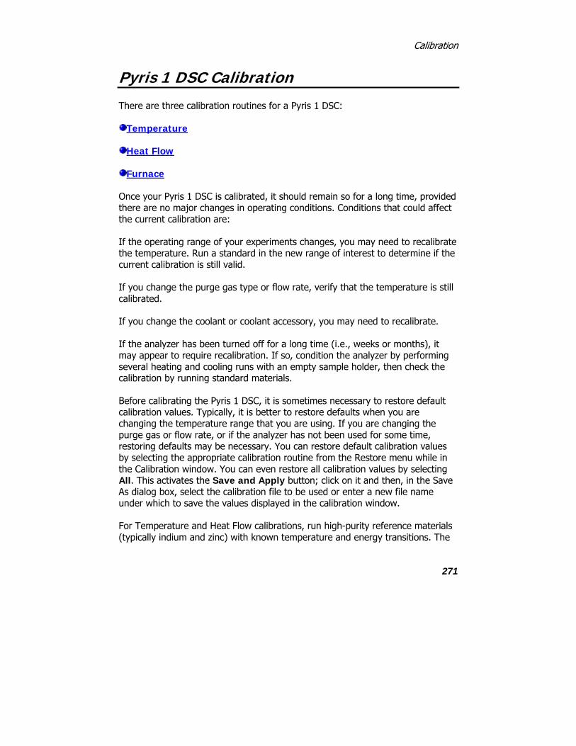
Calibration

271

Pyris 1 DSC Calibration

There are three calibration routines for a Pyris 1 DSC:

Temperature

Heat Flow

Furnace

Once your Pyris 1 DSC is calibrated, it should remain so for a long time, provided there are no major changes in operating conditions. Conditions that could affect the current calibration are:

If the operating range of your experiments changes, you may need to recalibrate the temperature. Run a standard in the new range of interest to determine if the current calibration is still valid.

If you change the purge gas type or flow rate, verify that the temperature is still calibrated.

If you change the coolant or coolant accessory, you may need to recalibrate.

If the analyzer has been turned off for a long time (i.e., weeks or months), it may appear to require recalibration. If so, condition the analyzer by performing several heating and cooling runs with an empty sample holder, then check the calibration by running standard materials.

Before calibrating the Pyris 1 DSC, it is sometimes necessary to restore default calibration values. Typically, it is better to restore defaults when you are changing the temperature range that you are using. If you are changing the purge gas or flow rate, or if the analyzer has not been used for some time, restoring defaults may be necessary. You can restore default calibration values by selecting the appropriate calibration routine from the Restore menu while in the Calibration window. You can even restore all calibration values by selecting All. This activates the Save and Apply button; click on it and then, in the Save As dialog box, select the calibration file to be used or enter a new file name under which to save the values displayed in the calibration window.

For Temperature and Heat Flow calibrations, run high-purity reference materials (typically indium and zinc) with known temperature and energy transitions. The

Pyris

272

data obtained from these runs are used in the Pyris software calibration routines to calibrate the Pyris 1 DSC. Once the analyzer is calibrated, it will remain calibrated even when the system is turned off, as long as there are no changes in the operating conditions.


Select the Temperature tab to display the Temperature page of the Calibration window. If you are restoring default calibration values, do so before completing the reference material sample runs.

To perform the Pyris 1 DSC Temperature calibration, complete a scan for each reference material under the same conditions that you run your samples. After each run is completed, perform a Peak Area calculation and include the Onset temperature. Record the H (J/g) and Onset results; you will need the Onset result for Temperature calibration and you can use the H result for Heat Flow calibration.

When all of the reference materials have been run and calculations performed, enter the reference material name, expected onset temperature, measured onset temperature, and calibration method name in the table on the Temperature calibration page. Click on the check box in the “Use” column for each reference that is to be used in the calibration.

When all of the information has been entered, click on the Save and Apply button to save the calibration values and apply them. Go on to the next calibration procedure or select Close to close the Calibration window and begin using the new calibration values.

If you are performing a Furnace calibration (for DDSC mode), it is essential to Save and Apply the new Temperature calibration first.

Heat Flow Calibration

Select the Heat Flow tab to display the Heat Flow page of the Calibration window. A Heat Flow calibration uses a single standard. The Heat Flow calibration value can be slightly modified by running a new reference sample while the existing calibration is applied.

To perform the Pyris 1 DSC Heat Flow calibration, complete a scan for the reference material under the same conditions that you run your samples or use

Calibration

273

one of the scans completed for the Temperature calibration. After the run is completed, perform a Peak Area calculation and record the H (J/g) result.

Enter the reference material name, expected H, the measured H, weight of the reference material, and calibration method name in the Calibration table.


Furnace Calibration

The Pyris 1 DSC Furnace calibration routine is used when your analyzer has the DDSC accessory installed. The calibration linearizes the Pyris 1 DSC furnace by matching the program temperature to the sensor temperature over the range that you enter. If you have just completed a Temperature calibration procedure, you must Save and Apply the new Temperature calibration before starting the Furnace calibration.

Select the Furnace tab to display the Furnace page of the Calibration window. Enter the minimum and maximum temperature limits, then select the Begin Calibration button and follow the instructions in the dialog box. To accept the Furnace calibration values, click on Save and Apply.

Quick Help | Pyris 1 DSC Hardware Help

Pyris

274

DSC 7 Calibration

There are three calibration routines for a DSC 7:

Temperature

Heat Flow

Furnace (DDSC only)

Once your DSC 7 is calibrated, it should remain so for a long time, provided there are no major changes in operating conditions. Conditions that could affect the current calibration and require you to recalibrate the DSC 7 are


If you adjust the Balance control on the analyzer, you may need to recalibrate. Always optimize the DSC 7 baseline before calibrating the analyzer.


If you change the coolant or coolant accessory, you may need to recalibrate.

If the analyzer has been turned off for a long time (i.e., weeks or months), it may appear to require recalibration. In this case, condition the DSC 7 by performing several heating and cooling runs with an empty sample holder, then check the calibration by running standard materials.

Before calibrating the DSC 7, it is sometimes necessary to restore default calibration values. Typically, it is better to restore defaults when you are changing the temperature range that you are using. If you are changing the purge gas or flow rate, or if the analyzer has not been used for some time, restoring defaults may be necessary. The Temperature calibration can be slightly modified by running a new reference sample while the existing calibration is applied. You can restore default calibration values by selecting the appropriate calibration routine from the Restore menu while in the Calibration window. You can even restore all calibration values by selecting All. This activates the Save and Apply button; click on it and then, in the Save As dialog box, select the

Calibration

275

calibration file to be used or enter a new file name under which to save the values displayed in the calibration window.

For Temperature and Heat Flow calibrations, run high-purity reference materials (typically indium and zinc) with known temperature and energy transitions. The data obtained from these runs are used in the Pyris software calibration routines to calibrate the DSC 7. Once the analyzer is calibrated, it will remain calibrated even when the system is turned off, as long as there are no changes in the operating conditions.



To perform the DSC 7 Temperature calibration, complete a scan for each reference material under the same conditions that you run your samples. After each run is completed, perform a Peak Area calculation and include the Onset temperature. Record the H (J/g) and Onset results; you will need the Onset result for Temperature calibration and you can use the H result for Heat Flow calibration.

When all of the reference materials have been run and calculations performed, enter the reference material name, expected onset temperature, measured onset temperature, and calibration method name in the table on the Temperature page. Click on the check box in the “Use” column for each reference that is to be used in the calibration.


If you are performing a Furnace calibration next (if your DSC 7 has the DDSC installed), it is essential to Save and Apply the new Temperature calibration first.


Select the Heat Flow tab to display the Heat Flow page of the Calibration window. A Heat Flow calibration uses a single standard. The Heat Flow

Pyris

276

calibration value can be slightly modified by running a new reference sample while the existing calibration is applied.

To perform the DSC 7 Heat Flow calibration, complete a scan for the reference material under the same conditions that you run your samples or use one of the scans completed for the Temperature calibration. After the run is completed, perform a Peak Area calculation and record the H (J/g) result.

Enter the reference material name, expected H, measured H, weight of the reference material, and calibration method name in the Calibration table.


Furnace Calibration

The Furnace Calibration is available for a DSC 7 if the DDSC accessory is installed. This calibration linearizes the DSC 7 furnace by matching the program temperature to the sensor temperature over the range that you enter. If you have just completed a Temperature calibration procedure, you must Save and Apply the new Temperature calibration before starting the Furnace calibration.

Select the Furnace tab to display the Furnace page of the Calibration window. Enter the minimum and maximum temperature limits, then select the Begin Calibration button and follow the instructions in the dialog box. To accept the Furnace calibration values, click on Save and Apply.

Quick Help | DSC 7 Hardware Help

Calibration

277

Pyris 6 DSC Calibration

There are two calibration routines for a Pyris 6 DSC:

Temperature

Heat Flow

It is recommended that a baseline correction be performed before temperature calibration.

The Pyris 6 DSC analyzer has been calibrated at the factory for both temperature and heat flow. Under normal conditions, the Pyris 6 DSC does not need temperature recalibration. Temperature calibration and heat flow calibration should be checked using the precrimped samples of indium and zinc before obtaining data. Some conditions that could affect the current calibration of the Pyris 6 DSC:

If the operating range of your experiments changes, you may need to recalibrate the temperature. Run a standard in the new range of interest to determine if the current calibration is valid.

If you change the purge gas type or flow type, verify that the temperature is still calibrated.

If you change the coolant, you may need to recalibrate.

If the Pyris 6 DSC has been turned off for a long time (i.e., weeks or months), it may appear to require recalibration. If so, condition the analyzer by performing several heating and cooling runs with an empty sample holder, then check the calibration by running standard materials.

Before calibrating the Pyris 6 DSC, it is sometimes necessary to restore default calibration values. Typically, it is better to restore defaults when you are changing the temperature range that you are using. If you are changing the purge gas or flow rate, or if the analyzer has not been used for some time, restoring defaults may be necessary. The Temperature calibration can be slightly modified by running a new reference sample while the existing calibration is applied. You can restore default calibration values by selecting the appropriate calibration routine from the Restore menu while in the Calibration window. You can even restore all calibration values by selecting All. This activates the Save

Pyris

278

and Apply button; click on it and then, in the Save As dialog box, select the calibration file to be used or enter a new file name under which to save the values displayed in the calibration window.

Note: After you restore the calibration for a Jade DSC or a Pyris 6 DSC and click Save and Apply to close the Calibration window, the sample purge gas values must be reapplied on the Control Panel.

For Temperature and Heat Flow calibrations, run high-purity reference materials (typically indium and zinc) with known temperature and energy transitions. The data obtained from these runs are used in the Pyris software calibration routines to calibrate the Pyris 6 DSC. Once the analyzer is calibrated, it will remain calibrated even when the system is turned off, as long as there are no changes in the operating conditions.



To perform the Pyris 6 DSC temperature calibration, complete a scan for each reference material under the same conditions that you use to run your samples. After each run is completed, perform a Peak Area calculation and include the Onset temperature. Record the H (J/g) and Onset results; you will need the Onset result for Temperature calibration and you can use the H result for Heat Flow calibration.

When all of the reference materials have been run and calculations performed, enter the reference material name, expected onset temperature, measured onset temperature, and calibration method name used in the table on the Temperature page. Click on the check box in the “Use” column for each reference that is to be used in the calibration.


Calibration

279


Select the Heat Flow tab to display the Heat Flow page of the Calibration window. A Heat Flow calibration uses a single standard. The Heat Flow calibration value can be slightly modified by running a new reference sample while the existing calibration is applied.

To perform the Pyris 6 DSC Heat Flow calibration, complete a scan for the reference material under the same conditions that you run your samples or use one of the scans completed for the Temperature calibration. After the run is completed, perform a Peak Area calculation and record the H (J/g) result.

Enter the reference material name, the expected H, the measured H, the weight of the reference material, and the calibration method name in the Calibration table.

When all of the information has been entered, click on the Save and Apply button to save the calibration values and apply them. Select Close to close the Calibration window and begin using the new calibration values.

Pyris

280

Jade DSC Calibration There are two calibration routines for a Jade DSC:

• Temperature

• Heat Flow

The Jade DSC analyzer has been pre-calibrated at the factory for both temperature and heat flow. Temperature calibration and heat flow calibration should be checked using the precrimped samples of indium and zinc before obtaining data. Some conditions that could affect the current calibration of the Jade DSC:

1. If the operating range of your experiments changes, you may need to recalibrate the temperature. Run a standard in the new range of interest to determine if the current calibration is valid.

2. If you change the purge gas type or flow type, verify that the temperature is still calibrated.

3. If you change the coolant, you may need to recalibrate.

4. If the Jade DSC has been turned off for a long time (i.e., weeks or months), it may appear to require recalibration. If so, condition the analyzer by performing several heating and cooling runs with an empty sample holder, then check the calibration by running standard materials.

Before calibrating the Jade DSC, it is sometimes necessary to restore default calibration values. Typically, it is better to restore defaults when you are changing the temperature range that you are using. If you are changing the purge gas or flow rate, or if the analyzer has not been used for some time, restoring defaults may be necessary. The Temperature calibration can be slightly modified by running a new reference sample while the existing calibration is applied. You can restore default calibration values by selecting the appropriate calibration routine from the Restore menu while in the Calibration window. You can even restore all calibration values by selecting All. This activates the Save and Apply button; click on it and then, in the Save As dialog box, select the calibration file to be used or enter a new file name under which to save the values displayed in the calibration window.

Calibration

281

Note: After you restore the calibration for a Jade DSC or a Pyris 6 DSC and click Save and Apply to close the Calibration window, the sample purge gas values must be reapplied on the Control Panel.

For Temperature and Heat Flow calibrations, run high-purity reference materials (typically indium and zinc) with known temperature and energy transitions. The data obtained from these runs are used in the Pyris software calibration routines to calibrate the Jade DSC. Once the analyzer is calibrated, it will remain calibrated even when the system is turned off, as long as there are no changes in the operating conditions.


Note: If you are restoring default calibration values, do so before completing the reference material sample runs.

1. From the Calibration dialog select the Temperature tab page.

Pyris

282

. The Temperature page displays.

2. To perform the Jade DSC temperature calibration, complete a scan for each reference material under the same conditions that you use to run your samples.

3. After each run is completed, perform a Peak Area calculation and include the Onset temperature.

4. Record the H (J/g) and Onset results; you will need the Onset result for Temperature calibration and you can use the H result for Heat Flow calibration.

5. When all of the reference materials have been run and calculations performed, enter the reference material name, expected onset

Calibration

283

temperature, measured onset temperature, and calibration method name used in the table on the Temperature page.

6. Click on the check box in the “Use” column for each reference that is to be used in the calibration.

7. When all of the information has been entered, click on the Save and Apply button to save the calibration values and apply them. Go on to the next calibration procedure or select Close to close the Calibration window and begin using the new calibration values.

Pyris

284


1. From the Calibration dialog, select the Heat Flow tab page.

tab. The Heat Flow page displays. A Heat Flow calibration uses a single standard. The Heat Flow calibration value can be slightly modified by running a new reference sample while the existing calibration is applied.

2. To perform the Jade DSC Heat Flow calibration, complete a scan for the reference material under the same conditions that you run your samples or use one of the scans completed for the Temperature calibration.

3. After the run is completed, perform a Peak Area calculation and record the H (J/g) result.

Calibration

285

4. Enter the reference material name, the expected H, the measured H, the weight of the reference material, and the calibration

method name in the Calibration table.

5. When all of the information has been entered, click on the Save and Apply button to save the calibration values and apply them. Select Close to close the Calibration window and begin using the new calibration values.

Pyris

286

DDSC Calibration

The Dynamic Differential Scanning Calorimetry (DDSC) accessory for the DSC 7 and the Pyris 1 DSC allows you to operate the analyzer as either a standard DSC 7 or Pyris 1 DSC or in DDSC mode. Upon installation of the DDSC, the analyzer is calibrated for Tp, the program temperature, and Ts, the sensor temperature.

NOTE: The DSC 7 or the Pyris 1 DSC with the DDSC accessory is calibrated only from the standard mode. Once you calibrate the sensor temperature, the DDSC mode will be calibrated automatically.

The calibration routines for an analyzer with a DDSC accessory are



Furnace Calibration

Once the calibration routines are performed, the temperature and heat flow calibrations should remain unchanged for a long time, provided there are no changes in the operating conditions of the instrument. Conditions that could affect the current calibration of the DSC 7 or Pyris 1 DSC with the DDSC accessory and require recalibration are

If the operating temperature range of your experiments changes, recalibration may be necessary. Run a reference material in the new range of interest to determine if the current calibration is valid.

If the Balance control is adjusted, recalibration may be necessary. Therefore, always optimize the baseline before the instrument is calibrated.

If the purge gas type or purge gas flow rate is changed, the calibration should be checked for highest accuracy. Switching between helium and another gas will require recalibration as well.

If you change the coolant or cooling accessory, recalibration may be necessary.

Since the temperature calibration is slightly dependent on scan rate for DDSC analyzers, final calibration should be performed at the scan rate that you will use for your experiments. As the scan rate is increased from the rate used for

Calibration

287

calibration, the transition temperature may change slightly. If you will be using a wide range of heating rates, or heating and cooling rates, it is better to calibrate at the slowest rate to be used. When operating in DDSC mode, it is best to calibrate at a slow rate of < 5°C/min.

If the instrument has been turned off for a long period of time (i.e., weeks or months), the instrument may appear to require recalibration. Condition the instrument by performing several heating and cooling runs with the sample holder empty and then check the calibration by running reference materials.

Pyris

288

TGA 7 Calibration

There are two calibration routines for a standard furnace and a high temperature furnace TGA 7:

Weight

Furnace

For a standard furnace TGA 7, there is an additional calibration routine:

Temperature

Once your TGA 7 is calibrated, it should remain so for a long time, provided there are no major changes in operating conditions. The conditions that could affect the current calibration are


If you install a new furnace, verify that the temperature is still calibrated.


If you install a new thermocouple or change the position of the thermocouple, verify that the temperature is still calibrated.

If you change the hangdown wire or sample pan, verify that the weight is still calibrated.

If the analyzer has been turned off for a long time (i.e., weeks or months), it may appear to require recalibration. In this case, condition the TGA 7 by performing several heating and cooling runs with an empty sample holder, then check the calibration by running standard materials.

Before calibrating the TGA 7, it is sometimes necessary to restore default calibration values. Typically, it is better to restore defaults when changing the temperature range that you are using. If you are changing the purge gas or flow

Calibration

289

rate, or if the analyzer has not been used for some time, you may need to restore defaults. The Temperature calibration can be slightly modified by running a new reference sample while the existing calibration is applied. You can restore default calibration values by selecting the appropriate calibration routine from the Restore menu while in the Calibration window. You can even restore all calibration values by selecting All. This activates the Save and Apply button; click on it and then, in the Save As dialog box, select the calibration file to be used or enter a new file name under which to save the values displayed in the calibration window.


For the TGA 7 Temperature calibration, run Curie point calibrations for high-purity reference materials. (For the high temperature furnace TGA 7 Temperature calibration, refer to ASTM Method E1582 for another procedure.) The data obtained from these runs are used in the Pyris software calibration routines to calibrate the TGA 7 temperature. Once the analyzer is calibrated, it will remain calibrated even when the system is turned off, as long as there are no changes in the operating conditions.


To perform the TGA 7 Temperature calibration, complete a scan for each reference material under the same conditions that you run your samples. After each run is completed, perform an Onset calculation at the end of the Curie point transition. Record the Onset temperature.

When all of the reference materials have been run and calculations performed, enter the reference material name, expected onset temperature, measured onset temperature, and calibration method name in the table on the Temperature Calibration page. Click on the check box in the “Use” column for each reference that is to be used in the calibration.


If you are performing a Furnace calibration next, it is essential to Save and Apply the new Temperature calibration first.

Pyris

290

Weight Calibration

In a Weight calibration, you compare the known weight of a reference material with the actual weight read from the TGA 7. The Weight calibration value can be slightly modified by recalibrating while the existing calibration is applied.

Enter the known weight of the reference material in the Weight page of the Calibration window, then select the Begin Calibration button and follow the instructions in the dialog boxes. You can cancel the calibration at any time by selecting the Cancel button in any dialog box.

Furnace Calibration

The TGA 7 Furnace calibration is a nine-point calibration between two specified temperature limits. It linearizes the TGA 7 furnace by matching the program temperature to the thermocouple temperature over the range that you enter.

If you have just completed a Temperature calibration procedure, you must Save and Apply the new Temperature calibration before starting the Furnace calibration.

Select the Furnace tab to display the Furnace page of the Calibration window. Enter the Minimum and Maximum temperature limits, then select the Begin Calibration button and follow the instructions in the dialog box. You can minimize the Instrument Application window while the TGA 7 furnace is being calibrated. To accept the Furnace calibration values, click on Save and Apply.

Quick Help | TGA 7 Hardware Help

Calibration

291

Pyris 6 TGA Calibration

There are three calibration routines for a Pyris 6 TGA:

Furnace

Temperature

Weight

The Pyris 6 TGA analyzer has been calibrated by the service engineer that installed it. Under normal conditions, the Pyris 6 TGA does not need temperature recalibration. If it is necessary to calibrate the Pyris 6 TGA, Furnace calibration must be performed before Temperature calibration. Temperature calibration should be checked using the two or three of the four reference materials provided and the weight calibration should be checked using the reference weight provided before performing any runs.

Once your Pyris 6 TGA is calibrated, it should remain so for a long time, provided there are no major changes in operating conditions. The conditions that could affect the current calibration are

If the operating temperature range of your experiments changes, you may need to recalibrate the temperature. Run a standard in the new range of interest to determine if the current calibration is still valid.


If you install a new sample thermocouple, or if the existing one has been disturbed, verify that the temperature is still calibrated.

If you change the sample pan, verify that the weight is still calibrated.

If the analyzer has been turned off for a long time (i.e., weeks or months), it may appear to require recalibration. In this case, condition the Pyris 6 TGA by performing several heating and cooling runs with an empty sample holder, then check the calibration by running standard materials.

Pyris

292

Before calibrating the Pyris 6 TGA, it is sometimes necessary to restore default calibration values. Typically, it is better to restore defaults when changing the temperature range used. If you are changing the purge gas or flow rate, or if the analyzer has not been used for some time, you may need to restore defaults. The Temperature calibration can be slightly modified by running a new reference sample while the existing calibration is applied. You can restore default calibration values by selecting the appropriate calibration routine from the Restore menu while in the Calibration window. You can even restore all calibration values by selecting All. This activates the Save and Apply button; click on it and then, in the Save As dialog box, select the calibration file to be used or enter a new file name under which to save the values displayed in the calibration window.

Furnace Calibration

The Pyris 6 TGA Furnace calibration is a nine-point calibration between two specified temperature limits. It linearizes the Pyris 6 TGA furnace by matching the program temperature to the thermocouple temperature over the range that you enter.

Unlike other analyzers, do not do a Temperature calibration before the Furnace calibration. The Furnace calibration is to be done first.

Select the Furnace tab to display the Furnace page of the Calibration window. Enter the Minimum and Maximum temperature limits, then select the Begin Calibration button and follow the instructions in the dialog box. You can minimize the Instrument Application window while the Pyris 6 TGA furnace is being calibrated. To accept the Furnace calibration values, click on Save and Apply.


For the Pyris 6 TGA Temperature calibration, run Curie point calibrations for the high-purity reference materials provided with the instrument. The data obtained from these runs are used in the Pyris software calibration routines to calibrate the Pyris 6 TGA temperature. Once the analyzer is calibrated, it will remain calibrated even when the system is turned off, as long as there are no changes in the operating conditions.


Calibration

293

To perform the Pyris 6 TGA Temperature calibration, you complete two scans for each reference material under the same conditions that you run your samples. The first run should use the lower scanning rate (e.g., 5°C/min) and the second run the higher scanning rate (e.g., 50°C/min). You must run at least two reference materials. After each run is completed, perform an Onset calculation at the end of the Curie point transition. Record the Onset temperature.

When all of the reference materials have been run and calculations performed, in the Temperature calibration page enter the reference material name, expected onset temperature, measured onset temperature, and the scanning rates used.

When all of the information has been entered, click on the Save and Apply button to save the calibration values and apply them.

Weight Calibration

In a Weight calibration, you compare the known weight of a reference material with the actual weight read from the Pyris 6 TGA. The Weight calibration value can be slightly modified by recalibrating while the existing calibration is applied.

Enter the known weight of the reference material in the Weight page of the Calibration window, then select the Begin Calibration button and follow the instructions in the dialog boxes. You can cancel the calibration at any time by selecting the Cancel button in any dialog box.

Quick Help | Pyris 6 TGA Hardware Help

Pyris

294

Pyris 1 TGA Calibration

There are three calibration routines for the Pyris 1 TGA:

Temperature

Weight

Furnace

Once your Pyris 1 TGA is calibrated, it should remain so for a long time, provided there are no major changes in operating conditions. The conditions that could affect the current calibration are

If the operating range of your experiments changes, you may need to recalibrate the temperature. Run a standard in the new range of interest to determine if the current calibation is still valid.

If you install a new furnace, verify that the temperature is calibrated.


If you install a new thermocouple or change the position of the thermocouple, verify that the temperature is still calibrated.

If you change the hangdown wire or sample pan, verify that the weight is still calibrated.

If the analyzer has been turned off for a long time (i.e., weeks or months), it may appear to require recalibration. In this case, condition the Pyris 1 TGA by performing several heating and cooling runs with an empty sample pan, then check the calibration by running standard materials.

Before calibrating the Pyris 1 TGA, it is sometimes necessary to restore the default calibration values. Typically, it is better to restore defaults when changing the temperature range that you are using. If you are changing the purge gas or flow rate, or if the analyzer has not been used for some time, you may need to restore defaults. The Temperature calibration can be slightly modified by running a new reference sample while the existing calibration is applied. You can restore default calibration values by selecting the appropriate calibration routine from

Calibration

295

the Restore menu while in the Calibration window. You can even restore all calibration values by selecting All. This activates the Save and Apply button, click on it and then, in the Save As dialog box, select the calibration file to be used or enter a new file name under which to save the values displayed in the calibration window.


For the Pyris 1 TGA Temperature calibration, run Curie point calibrations for high-purity reference materials. (For the high-temperature furnace Pyris 1 TGA Temperature calibration, refer to ASTM Method E1582 for another procedure.) The data obtained from these runs are used in the Pyris software calibration routines to calibrate the Pyris 1 TGA temperature.


To perform the Pyris 1 TGA Temperature calibration, complete a scan for each reference material under the same conditions that you will run your samples. After each run is completed, perform an Onset calculation at the end of the Curie point transition. Record the Onset temperature.

When all of the reference materials have been run and calculations performed, enter the reference material name, expected onset temperature, measured onset temperature, and calibration method name in the table on the Temperature page. Click on the check box in the "Use" column for each reference that is to be used in the calibration.


If you are performing a Furnace calibration next, it is essential to Save and Apply the new temperature calibration first.

Weight Calibration

In a Weight calibration, you compare the known weight of a reference material with the actual weight read from the Pyris 1 TGA. The Weight calibration value can be slightly modified by recalibrating while the existing calibration is applied.

Pyris

296

Enter the known weight of the reference material in the Weight page of the Calibration window, then select the Begin Calibration button and follow the instructions in the dialog boxes. The instructions are slightly different for a Pyris 1 TGA with an autosampler.

Furnace Calibration

The Pyris 1 TGA Furnace calibration is a nine-point calibration between two specified temperature limits. It linearizes the Pyris 1 TGA furnace by matching the program temperature to the thermocouple temperature over the range that you enter.

NOTE: If you have just completed a Temperature calibration procedure, you must Save and Apply the new Temperature calibration before starting the Furnace calibration.

Select the Furnace tab to display the Furnace page of the Calibration window. Enter the Minimum and Maximum temperature limits, then select the Begin Calibration button and follow the instructions in the dialog box. You can minimize the Instrument Application window while the Pyris 1 TGA furnace is being calibrated so you can use other applications on the computer. To accept the Furnace calibration values, click on Save and Apply.

Quick Help

Calibration

297

DMA 7e Calibration

There are six calibration routines for a DMA 7e:

DMA Calibration

Height

Force

Eigendeformation

Temperature

Furnace

All calibrations are performed by a Service Engineer upon installation of your DMA 7e so it is not necessary for you to perform a complete calibration when you begin to use your analyzer. Periodic checking of the calibration is all that is needed to verify accurate calibration. Once the DMA 7e is calibrated, it should remain so for a long time, provided there are no changes in the instrument’s operating conditions. The analyzer remains calibrated even when it is turned off. Conditions that could affect the current calibration are

If the operating temperature range of your experiments changes, you may need to recalibrate the temperature axis. Check the temperature calibration in the range of interest (to determine if the current calibration is still valid) by measuring the melting point of a reference material.

If the purge gas or purge gas flow rate is changed, the temperature calibration should be checked.

If a new furnace is installed, the temperature calibration should be checked.

If a new thermocouple is installed or if the position of the thermocouple is changed, the temperature calibration should be checked.

The eigendeformation calibration should be checked and performed if the sample tube and/or probe is changed and the samples being analyzed are very stiff (that is, a high modulus of >10 GPa).

Pyris

298

If a different measuring system is installed, the temperature and other calibrations should be checked.

Before calibrating the DMA 7e, it is sometimes necessary to restore default calibration values. You can restore default calibration values by selecting the appropriate calibration routine from the Restore menu while in the Calibration window. You can even restore all calibration values by selecting All. This activates the Save and Apply button; click on it and then, in the Save As dialog box, select the calibration file to be used or enter a new file name under which to save the values displayed in the calibration window.

DMA Calibration

DMA Calibration performs necessary operations in the firmware and generates lookup tables stored in memory. Run the DMA Calibration with a 3-point bending measuring system installed.

Select the DMA tab in the Calibration window to display the DMA page. Click on Begin Calibration, remove any samples, lower the probe, raise the furnace assembly, and click on OK in the dialog box and calibration begins. Progress of the calibration is indicated by the elapsed time displayed. When complete, click on OK. To perform the next calibration, Height, you must select Save and Apply to save the calibration values and apply them.

Height Calibration

This procedure calibrates the displacement transducer that is used to measure the position and amplitude (ordinate) axis of the DMA 7e. To perform a Height calibration, you need the sapphire height displacement standard shipped with the instrument. Measure the height of the standard.

Select the Height tab in the Calibration window to display the Height page. Click on Begin Calibration. Prepare the analyzer for zero reading by removing any samples on the sample platform. Press the Probe Up button on the analyzer and check for any samples on the sample platform. Press Probe Down to lower the probe until it rests on the sample platform. Click on OK. After the Y signal has stabilized, select OK if you want the current Y value entered as the new zero value. Calibration sets the location of the empty sample platform as 0 mm.

You then place the displacement standard on the sample platform and lower the probe to rest on the standard. Wait for the Y signal to stabilize and then select

Calibration

299

OK to save the height calibration value. To accept the new height factor, Save and Apply.

Force Calibration

Select this tab to calibrate the force motor that is used to apply the static and dynamic forces to the sample. To perform the Force calibration, you need to 50-g-force calibration reference material and weight platform shipped with the instrument.

Select the Force tab in the Calibration window to display the Force page. Click on Begin Calibration, remove any sample from the platform, install the weight tray, and place the 50-g weight on the tray. When calibration is complete, remove the weight and the weight tray and the new force value is saved automatically.

Eigendeformation Calibration

This procedure calibrates the very small movement of the analyzer itself when large forces are applied. After performing the calibration, the compliance of the system is subtracted from the probe position signal. Increasing force with no sample present will yield zero displacement. This calibration should be performed after Height and Force calibration.

Select the Eigendeformation tab in the Calibration window to display the Eigendeformation page. Click on Begin Calibration, remove any sample from the platform, lower the probe, and wait for the calibration. You will then insert the steel reference material, lower the probe, and wait for the calibration to complete. Click on Save and Apply to accept the eigendeformation calibration values.


This one-point temperature calibration allows you to run one reference material to match the thermocouple temperature and the sample temperature. In this calibration, the onset melting temperature for indium is determined using the 3-point bending measuring system.

Select the Temperature tab in the Calibration window to display the Temperature page. To perform the DMA 7e Temperature calibration, complete a scan for indium reference material under the same conditions that you run your samples.

Pyris

300

After the run is completed, perform an Onset calculation and record the Onset temperature. Enter the reference material name, expected onset temperature, measured onset temperature, and calibration method name in the Calibration table. Click on the check box in the Use column. Select Save and Apply to send the new calibration value to the analyzer and save the calibration file.

Furnace Calibration

The DMA 7e Furnace calibration is a nine-point calibration between two specified temperature limits. It linearizes the DMA 7e furnace by matching the program temperature to the thermocouple temperature over the range that you enter.

Perform a Furnace calibration after a Temperature calibration. Select the Furnace tab in the Calibration window to display the Furnace page. Enter the Minimum and Maximum temperature limits, then select Begin Calibration and follow the instructions in the dialog box. To accept the Furnace calibration values, click on Save and Apply.

Calibration

301

TMA 7 Calibration

There are five calibration routines for the TMA 7:

Height

Force

Eigendeformation

Temperature

Furnace

All calibrations are performed by a Service Engineer upon installation of your TMA 7 so it is not necessary for you to perform a complete calibration when you begin to use your analyzer. Periodic checking of the calibration is all that is needed to verify accurate calibration. Once the TMA 7 is calibrated, it should remain so for a long time, provided there are no changes in the instrument’s operating conditions. The analyzer remains calibrated even when it is turned off. Conditions that could affect the current calibration are

Operating temperature range of your experiments changes. Check the temperature calibration in the range of interest to determine if the current calibration is still valid.

Purge gas or purge gas flow rate is changed.

New furnace is installed.

New thermocouple is installed or the position of the thermocouple is changed.

The Eigendeformation calibration should be checked and performed if the sample tube and/or probe is changed and the samples being analyzed are very stiff.

Before calibrating the TMA 7, it is sometimes necessary to restore default calibration values. You can restore default calibration values by selecting the appropriate calibration routine from the Restore menu while in the Calibration window. You can even restore all calibration values by selecting All. This activates the Save and Apply button; click on it and then, in the Save As dialog

Pyris

302

box, select the calibration file to be used or enter a new file name under which to save the values displayed in the calibration window.

Height Calibration

This procedure calibrates the displacement transducer that is used to measure the position and amplitude (ordinate) axis of the TMA 7. To perform a Height calibration, you need the sapphire height displacement standard shipped with the instrument. Measure the height of the standard.

Select the Height tab in the Calibration window to display the Height page. Click on Begin Calibration, prepare the analyzer for zero reading by removing any samples on the sample platform. Click on OK. Lower the probe until it rests on the sample platform. After the Y signal has stabilized, select Apply if you want the current Y value entered as the new zero value. Calibration sets the location of the empty sample platform as 0 mm.

You then place the displacement standard on the sample platform and lower the probe to rest on the standard. Wait for the Y signal to stabilize and then select Save and Apply to save the height calibration values and apply them.

Force Calibration

Select this tab to calibrate the force motor that is used to apply the static force to the sample. To perform the Force calibration, you need to 50-g-force calibration reference material and weight platform shipped with the instrument.

Select the Force tab in the Calibration window to display the Force page. Click on Begin Calibration, remove any sample from the platform, install the weight tray, and place the 50-g weight on the tray. When calibration is complete, remove the weight and the weight tray and the new force value is saved automatically.

Eigendeformation Calibration

This procedure calibrates the very small movement of the analyzer itself when large forces are applied. After performing the calibration, the compliance of the system is subtracted from the probe position signal. Increasing force with no sample present will yield zero displacement. This calibration should be performed after Height and Force calibration.

Calibration

303

Select the Eigendeformation tab in the Calibration window to display the Eigendeformation page. Click on Begin Calibration, remove any sample from the platform, lower the probe, and wait for the calibration. You will then insert the steel reference material, lower the probe, and wait for the calibration to complete. Click on Save and Apply to accept the eigendeformation calibration values.


This one-point temperature calibration allows you to run one reference material to match the thermocouple temperature and the sample temperature. In this calibration, the onset melting temperature for indium is determined using the penetration probe.

Select the Temperature tab in the Calibration window to display the Temperature page. To perform the TMA 7 Temperature calibration, complete a scan for indium reference material under the same conditions that you run your samples. After the run is completed, perform an Onset calculation and record the Onset temperature. Enter the reference material name, expected onset temperature, measured onset temperature, and calibration method name in the Calibration table. Click on the check box in the Use column. Select Save and Apply to send the new calibration value to the analyzer and save the calibration file.

Furnace Calibration

The TMA 7 Furnace calibration is a nine-point calibration between two specified temperature limits. It linearizes the TMA 7 furnace by matching the program temperature to the thermocouple temperature over the range that you enter.

Perform a Furnace calibration after a Temperature calibration. Select the Furnace tab in the Calibration window to display the Furnace page. Enter the Minimum and Maximum temperature limits, then select Begin Calibration and follow the instructions in the dialog box. To accept the Furnace calibration values, click on Save and Apply.

Quick Help | TMA 7 Hardware Help

Pyris

304

DTA 7 Calibration

There are three calibration routines used to calibrate the DTA 7:

Temperature

Heat Flow

Furnace

All calibrations are performed by a Service Engineer upon installation of your DTA 7 so it not necessary for you to perform a complete calibration when you begin to use your analyzer. Once the calibration is performed, the analyzer will be continuously calibrated, even when the system is turned off. Unless major changes to the analyzer’s condition are made, the DTA 7 should remain calibrated.

All three calibrations can be performed separately or together. The Furnace calibration must be performed after the Temperature calibration. The recommended calibration procedure is to perform a 2-standard Temperature calibration when the instrument is first installed or when the DTA 7 sample and reference thermocouples are changed. Temperature calibration should be performed if either the furnace thermocouple or the furnace is changed. Conditions that could affect the furnace, temperature, or energy calibration of the DTA 7 are

Operating temperature range of your experiments changes. Check the temperature calibration in the range of interest to determine if the current calibration is still valid.

Slope control is adjusted. Always optimize the DTA 7 baseline before the instrument is calibrated.

Purge gas type or flow rate changes. Calibration should be checked for highest accuracy.

New furnace or new furnace thermocouple is installed. The Temperature and Furnace calibrations should be performed again.

New pair of sample and reference thermocouples are installed. Temperature calibration should be performed again.

Calibration

305

Instrument has been turned off for a long time (i.e., weeks or months). It may appear to need recalibration. Condition the DTA 7 by performing several heating and cooling runs with the sample and reference cups empty and then check the calibration by running standard reference materials.

NOTE: The Temperature calibration is dependent on scan rate. Therefore, the final calibration should be performed at the scan rate that you will use for your experiments.

As the scan rate is increased from the rate used for calibration, the transition temperature may change slightly. If you will be using a wide range of heating and cooling rates, it is better to calibrate at the slowest rate you will be using.

Before calibrating the DTA 7, it is sometimes necessary to restore default calibration values. You can restore default calibration values by selecting the appropriate calibration routine from the Restore menu while in the Calibration window. You can even restore all calibration values by selecting All. This activates the Save and Apply button; click on it and then, in the Save As dialog box, select the calibration file to be used or enter a new file name under which to save the values displayed in the calibration window.


This two-point calibration consists of running two high-purity standards (shipped with the instrument) and measuring the melt onset for each material. The measured onset temperature is compared with the expected onset temperature to calibrate the temperature axis over a very broad temperature range.

To perform the DTA 7 Temperature calibration, complete a scan for aluminum under the same conditions that you run your samples. After the run is completed, perform a Peak Area with Onset calculation and record the Onset temperature. Do the same for the gold reference material. Select the Temperature tab in the Calibration window to display the Temperature page. Enter the information in the Temperature page and select Save and Apply to send the new calibration values to the analyzer and save the calibration file.


Two high-purity standards are used to calibrate H. This calibration is used to run in the DSC mode or when data collected in the DTA mode needs to be converted to Sample Heat Flow data.

Pyris

306

To perform the Heat Flow calibration, accurately weigh the reference material. The accuracy and precision to which you weigh the reference material relates directly to the accuracy and precision of the energy measurements made on the DTA 7. Complete a scan of the reference material and perform a Peak Area calculation and note the H result. Select the Heat Flow tab in the Calibration window to display the Heat Flow page. Enter the information and select Save and Apply to send the new calibration values to the analyzer and the save the calibration file.

Furnace Calibration

This calibration performs a nine-point temperature calibration between user-selected limits. It must be performed after the Temperature calibration. Remove the cups from the sample and reference holders. Select the Furnace tab in the Calibration window to display the Furnace page and enter Minimum and Maximum temperatures. Click on Begin Calibration and the Furnace calibration will start; it takes up to 2.5 hours. Select Save and Apply to send the new calibration values to the analyzer and save the calibration file.

307

Methods Plus

Pyris

308

Method Actions and Events

By selecting different actions and events in your method, you can switch purge gases and flow rates, equilibrate before the run starts or during any program step, trigger actions based on signals to or from an external relay box, and time when you want actions to occur during the method.

What do you want to do?

Switch Purge Gases and Flow Rates

Equilibrate a signal

Use an external relay action or event

Time when an action will occur

Temperature when an action will occur

Combine events for a given action using AND/OR statements

Modify actions or events

Gas Switch Actions To switch purge gases or flow rates in your method:

Display the Initial State page of the method if you want to switch purge gases or flow rates before the run begins. Or, display the Program page of the method if you want the gas switch action to occur during one of the program steps.

Right-click to display the pop-up menu and select Add Action. Select Switch Gases.

In the Gas Switch action dialog, select the following parameters. The values displayed here are the default gas and flow rate selected in Preferences.

Parameter Description

Methods Plus

309

Purge Gas Click on the arrow to display the drop-down list of available gases. For a TAGS, the choices in the drop-down list are all available gases plus the option Gas Off. The gases selected in Preferences are marked with an asterisk and appear at the top of the list. For a GSA 7, the choices in the drop-down list are the two gases specified in Preferences (when editing a method in Data Analysis application, the choice of gases is the entire list). The gases selected in Preferences are marked with an asterisk and appear at the top of the list. If there is no gas accessory attached, then the name of the gas used at the start of the run is displayed in gray. Only the Air Cooling Unit is available for Diamond TG/DTA, Diamond TMA Standard Temperature, and Diamond TMA High Temperature.

Flow Rate The default purge gas flow rate displayed was entered in Preferences. This field is read only for a GSA 7 and no gas switching accessory. For a TAGS, increase or decrease the flow rate by entering a new value or using the spin buttons.

Select the event that you want to trigger the gas switch action to occur. For more information on these events, see Table 2.

Equilibration Events

The parameters in this dialog depend on the analyzer. In general, when you select an equilibration event, Pyris will monitor the addressed signal from the analyzer until it fluctuates within the specified criterion for 20 seconds (10 consecutive readings, each 2-s intervals).

NOTE: You can select one or more equilibration events. Use AND statements to specify that all events must occur before the run begins. Use OR statements to specify that only one of the events must occur before the run begins. For more information on using these statements, see Combining Events with AND/OR Statements.

To specify an equilibration event in your method:

Display the Initial State page of the method if you want to specify the equilibration event before the run begins. Or, display the Program page of the method if you want specify the event during one of the program steps.

Pyris

310

Right-click to display the pop-up menu and select Add Action. Select the action that will be triggered when the equilibration event occurs. The choices of actions are Start Run (Initial State only), Stop Run (Program page only), Switch Gases, and Trigger an External Action.

If you selected the actions of Switch Gases or Trigger an External Action, you will need to specify additional information in the next dialog that appears.

When the dialog appears that asks you to select an event, click on A Signal Equilibrates.

In the Equilibration Event dialog, select the signal that needs to be equilibrated. The signals that appear in this dialog depend on the analyzer. The different signals are described in the table below.

Signal Analyzer Description

Sample Temperature all analyzers This is the temperature of the thermocouple and the sample's environment in degrees Celsius.

Temperature all analyzers This is the temperature you specify for the program in degrees Celsius.

Heat Flow DSC analyzers For DSC analyzers, the Y signal is Heat Flow. Units are in milliwatts (mW).

Normalized Heat Flow DSC analyzers This is the heat flow signal divided by the sample weight. Units are in Weight/grams (W/g).

Weight TGA analyzers For TGA analyzers, the Y signal is weight in milligrams (mg).

Unsubtracted Delta T DTA 7 For the DTA 7, this is the Delta T signal before baseline subtraction is performed. Delta T is the difference in temperature

Methods Plus

311

between the sample and an inert reference material.

Probe Position Diamond TMA,

TMA 7

This is the average position of the probe tip (in millimeters) during the run.

Height% Diamond TMA,

TMA 7

The amount by which the height measured by the analyzer can fluctuate from the Height value measured and entered by the user.

Select a Criterion value. This is a plus or minus value that represents the amount the signal can fluctuate up or down when equilibration occurs.

If desired, you can use a Setpoint by checking the box and entering a value. A setpoint defines a target value for equilibration. For example, if you select a Setpoint at a temperature of 50 °C and the criterion is 0.1, the equilibration event will only occur if the signal equilibrates between the range of 49.9 to 50.1 °C. If the signal equilibrates at a different temperature, for example 40 °C, the equilibration event will not occur because it is not at the specified setpoint.

Select whether you want the signal to be monitored at the beginning of the segment or at a specified time into the segment and enter the time in minutes.

Cross-Boundary Events

In general, when you select a cross-boundary event, the software will monitor the addressed signal from the analyzer and cause the specified action to occur if the signal crosses an upper or lower boundary. To specify a cross-boundary event in your method:

Display the Initial State page of the method if you want to specify the cross-boundary event before the run begins. Or, display the Program page of the method if you want to specify the event during one of the program steps.

Right-click to display the pop-up menu and select Add Action. Select the action that will be triggered when the cross-boundary event occurs. The choices of actions are Start Run (Initial State only), Stop Run (Program page only), Switch Gases, and Trigger an External Action.

Pyris

312


When the dialog appears that asks you to select an event, click on A Signal Crosses a Boundary.

In the Cross-Boundary Event dialog, select the signal that needs to be monitored. The signals that appear in this dialog depend on the analyzer. The different signals are described in the table below.

Signal Analyzer Description

Sample Temperature all analyzers This is the temperature of the thermocouple and the sample's environment in degrees Celsius.

Temperature all analyzers This is the temperature you specify for the program in degrees Celsius.

Heat Flow DSC analyzers For DSC analyzers, the Y signal is Heat Flow in milliwatts (mW).

Normalized Heat Flow DSC analyzers This is the heat flow signal divided by the sample weight. Units are in Weight/grams (W/g).

Weight TGA analyzers For TGA analyzers, the Y signal is weight in milligrams (mg).

Probe Position Diamond TMA This is the average position of the probe tip (in millimeters) during the run.

Height% Diamond TMA The amount by which the height measured by the analyzer can fluctuate from the Height value measured and entered by the user.

Methods Plus

313

You can specify both an upper boundary and lower boundary, or just one boundary. Check the appropriate boxes and enter a value. The action you specified will only occur if the signal crosses the specified boundaries.

Select whether you want the signal to be monitored at the beginning of the segment or at a specified time into the segment and enter the time in minutes.

External Relay Actions and Events

One of the advanced features of the software is operation of your system and accessories in conjunction with an external relay box. The software is capable of both sending and receiving signals from the external relay box. You can specify an external relay action, which will trigger an action to occur by switching a channel on the external relay on or off before the run or during any program step. Or, you can specify an external relay event, which means that an action associated with a program step will only occur if the software receives a signal from the external relay box.

NOTE: External Relay actions and events are not available for the DMA or DTA.

To specify an external relay ACTION in your method:

Display the Initial State page of the method if you want to specify the external relay before the run begins. Or, display the Program page of the method to specify the external relay during one of the program steps.

Right-click to display the pop-up menu and select Add Action. Select Trigger an External Action.

Select the event that you want to trigger the external relay action to occur.

In the External Trigger Action dialog, click on the drop-down list to select the channel on the external relay box to switch on or off. To specify an external relay EVENT in your method:

Display the Initial State page of the method if you want to specify the external relay before the run begins. Or, display the Program page of the method to specify the external relay during one of the program steps.

Right-click to display the pop-up menu and select Add Action. Select the action that will be triggered when the external relay event occurs. The choices of

Pyris

314

actions are Start Run (Initial State only), Stop Run (Program page only), Switch Gases, and Trigger an External Action.

NOTE: For advanced applications, the software allows you to specify that both an external relay action should switch one channel on or off and that this action should occur based on an external relay event from another channel.


When the dialog appears that asks you to select an event, click on An External Event occurs.

In the External Trigger Event dialog, click on the drop-down list to select the channel on the external relay box to switch on or off.

Timed Events

When you select a timed event, the action will occur when a specified time is reached after a program segment starts. You have the option of timing any of the following actions: Start Run (Initial State only), Stop Run (Program page only), Switch Gases, and Trigger an External Event. To specify timed events in your method

Display the Initial State page of the method if you want to specify the timed event before the run begins. Or, display the Program page of the method to specify the timed event during one of the program steps.

Right-click to display the pop-up menu and select Add Action. Select the action that will be triggered when the specified time is reached. The choices of actions are Start Run (Initial State only), Stop Run (Program page only), Switch Gases, and Trigger an External Action.


When the dialog appears that asks you to select an event, click on A Specified Time is reached.

In the Timed Event dialog, specify the amount of time to wait in the program segment before the action occurs.

Methods Plus

315

Combining events with AND/OR statements To select one event AND another event for a given action

In some cases, you may want an action to occur when more than one condition is met. For example, you can switch gases when an external event occurs and a specified time is reached. Both of these events must occur before the action takes place.

This example would read as follows: Switch the Gas to Nitrogen at 20.0 ml/min

...and the Time is >=2.000 min

...and the External Channel 1 is On

Click on the action to highlight it, then click the right mouse button.

A pop-up menu appears. Select Add an Event.

In the next dialog that appears, select an additional event. To select one event OR another event for a given action

In some cases, you may want an action to occur when only one of multiple events takes place. For example, you may want to start the run either when the desired signal is equilibrated or when a specified time is reached. In this case, you need to duplicate the action by selecting it again, each time with a different event selection. The example would read as follows:

Start the Run

...if the Temperature Equilibrates Within +/ -1.000e-002

Start the Run

...if the Time is >=1.000 min

Pyris

316

Modifying Actions and Events To modify actions and events

Position the mouse cursor in the white program box and click the right mouse button.

A pop-up menu appears. Select one of the following commands:

Use this command in the pop-up menu... To do this...

Edit an Item To change the conditions associated with an action or event

Delete an Item To delete an action or event

Change an Item To select a different action or event

Temperature Events

When you select a Temperature event, the action will occur when a specified temperature is reached after a program segment starts. You have the option of selecting temperature with any of the following actions: Stop Run (Program page only), Switch Gases, and Trigger an External Event. To specify temperature events in your method

Display the Program page of the method to specify the temperature event during one of the program steps.

Right-click to display the pop-up menu and select Add Action. Select the action that will be triggered when the specified temperature is reached. The choices of actions are Stop Run (Program page only), Switch Gases, and Trigger an External Action.


Methods Plus

317

When the dialog appears that asks you to select an event, click on A Specified Temperature is reached.

In the Temperature Event dialog, specify the temperature to reach in the program segment before the action occurs.

Pyris

318

Initial State Page

The Initial State page appears when you select the Initial State tab of the Method Editor. On this page, you specify the initial conditions that are necessary before data is collected. This page is divided into the following sections:

Pre-Run Actions

Set Initial Values

Data Collection

Baseline File

Pre-Run Actions

In this section, you can select pre-run actions and events. An action defines what will occur during system initialization. For each action, you select one or more events that will cause that action to happen.

Table 1: Actions you can select on the Initial State page

Action What the action means

Start Run

You can start the run when one or more of the available events has occurred. Your options are to start the run when equilibration conditions have been reached, at a specified time, immediately, or when a signal is received from an external relay box.

Switch Gases You can switch to another purge gas or change the gas flow rate if your system is using a GSA 7, TAGS, or Air Cooling Unit for changing purge gases. On the Initial State page, the gas and flow rate selected are used during system initialization.

NOTE: On the Program page, the purge gas and flow rate can be changed in a gas program. You can also change the purge gas in real time by selecting a different gas in the Purge Gas field in the control panel.

Methods Plus

319

Trigger External Action This action will trigger a signal to a channel on an external relay box or an X-10 box. (This item is not available for the DMA or DTA.)

Table 2: Events you can select on the Initial State page

Event What the event means

A Signal equilibrates In general, when you select an equilibration event, the software will monitor the addressed signal from the analyzer until the peak-to-peak range of the signal is within the specified criterion for 20 seconds (10 consecutive readings, each 2-s intervals)

An External Event occurs

A signal is received from a channel on an external relay box or an X-10 box that triggers the action to occur. (This item is not available for the DMA or DTA.)

A Specified Time is reached

The action will occur once a specified time after the program segment starts.

Action occurs Immediately

The action will occur immediately when the program segment starts.

To select pre-run actions and events

Position the mouse cursor in the Pre-Run Actions section and click the right mouse button.

A pop-up menu appears. Select Add an Action.

A dialog appears that asks you to select an action. For information on each action, refer to Table 1 above.


Pyris

320

A dialog appears that asks you to select an event. For information on each event, refer to Table 2 above.








Set Initial Values Section Temperature

This field displays the initial temperature, i.e., the temperature of the thermocouple and the sample’s environment when the run starts. The default value displayed is the Load Temperature value entered in the Instrument page in Preferences. Type a new value or use the spin buttons to increase or decrease the displayed temperature in 5°C steps. This value is used in the first step of the method program on the Program page. Y Initial

Enter the initial ordinate (Y) value. Type the value or use the spin buttons to increase or decrease the displayed value in 5-mW steps.(This item is not available for the Diamond TG/DTA.)

Data Collection Section Sample Rate (DSC 7, Pyris 1 DSC, DTA 7)

Select the sample rate of Standard or Fast from the drop-down list box. This is the rate at which data are collected throughout the run. The standard data collection rate is 5 points per second; the fast rate is 20 points per second. Proper selection of a sample rate will increase the efficiency of the analysis. Generally, the slower scanning rate improves peak resolution while the fast scanning rate improves the usable sensitivity. The number of points saved in the date file also depends on the Data Sampling Options in the Step Details section of the Program page.

Methods Plus

321

Baseline File Section

Baseline subtraction performs a linear subtraction of the instrument baseline from a curve to improve the resolution of the transition of interest. Instrument baseline is established by placing empty sample pans in the sample and reference holders and performing a run under similar conditions that you run your samples. The data file saved is a baseline file. One should scan the analyzer under the proposed experimental conditions to check the curvature and noise level of the instrument baseline before analyzing samples. When you are going to run a sample, you can have the software perform a baseline subtraction using a baseline file that you collected. The Baseline File section of the Initial State page contains the following parameters: Use Baseline Subtraction check box

Click on the check box to activate Baseline Subtraction. The baseline file selected here is subtracted from the data as it is collected to optimize the data. When you select Baseline Subtraction, the Browse button becomes selectable. Directory

Displays the drive and directory in which the baseline file is stored. You cannot enter the drive/directory directly; you must use the Browse button to find and select the drive\directory. File Name

Enter the name of the baseline file to be used for the run or select the file from the Browse box. Browse

Activated when you click on the Baseline Subtraction check box. If you want to select a directory other than the default for storing the data file, click on the Browse button to display the Browse dialog box.

Pyris

322

Initial State Page


Pre-Run Actions

Set Initial Values

Pre-Run Actions




Start Run


Switch Gases You can switch to another purge gas or change the gas flow rate if your system is using a GSA 7 or a TAGS for changing purge gases. On the Initial State page, the gas and flow rate selected are used during system initialization.

NOTE: On the Program page, the purge gas and flow rate can be changed in a gas program. You can also change the purge gas in real time by selecting a different gas in the Purge Gas field in the control panel.

Methods Plus

323





A Specified Temperature is reached

The action will occur at the specified temperature.







If you selected the action of Switch Gases, you will need to specify additional information in the next dialog that appears.







Pyris

324



This field displays the initial temperature, i.e., the temperature of the thermocouple and the sample’s environment when the run starts. The default value displayed is the Load Temperature value entered in the Instrument page in Preferences. Type a new value or use the spin buttons to increase or decrease the displayed temperature in 5°C steps. This value is used in the first step of the method program on the Program page. Static Force or Static Stress

The static force should be sufficient to keep the probe in continuous contact with the sample during the entire analysis. Static force is usually 15% greater than the dynamic force. The static force is held constant in a temperature scan, a time (isothermal) scan, and a frequency scan. In a dynamic stress scan, the static force changes proportionally to the increasing dynamic force to assure that the sample remains in tension throughout the analysis. Enter the initial value into the field or use the spin buttons to increase or decrease the displayed static force in 10-mN steps. If you choose to report stress (selected in Preferences), then the value is in kPa. This value is displayed in the first step of the method program on the Program page. Dynamic Force or Dynamic Stress

The dynamic force should be sufficient to produce an initial displacement amplitude of 5 – 50 m. Dynamic force is held constant in a temperature scan, a time (isothermal) scan, and a frequency scan. It varies in a dynamic stress scan and is absent in a static force scan and a creep-recovery scan. Enter the initial value into the field or use the spin buttons to increase or decrease the displayed dynamic force in 10-mN steps. If you choose to report stress (selected in Preferences), then the value is in kPa. Frequency

Most applications use 1 Hz. This field displays the initial frequency at which the dynamic force is applied. The frequency is held constant in a temperature scan, a time (isothermal) scan, and a dynamic stress scan. There is no frequency in a static force scan or a creep-recovery scan. You cannot enter a value into the field; use the spin buttons to increase or decrease the displayed frequency in 0.2-Hz steps. This value is displayed in the first step of the method on the Program page. DMA 7e Set Controls

Methods Plus

325

Click on the Set Controls button to display an additional box for entering initial static force control parameters (tension control and position control) and dynamic force control parameters (stress control, strain control, and amplitude control). You can also turn off dynamic force in this box so that only static force applies. The DMA 7e is like a TMA 7 in this state. When a Creep Recovery or a Static Stress Scan method is used, or when Dynamic Force is turned off, there are no controls available on this window. When a Dynamic Stress Scan method is used, there are no Dynamic Controls available.

Top

Pyris

326

Diamond TMA Initial State Page


Pre-Run Actions

Set Initial Values

Set TMA Program

Baseline File

Pre-Run Actions




Start Run


Switch Gases You can switch to another purge gas or change the gas flow rate if your system is using a GSA 7 or a TAGS for changing purge gases. On the Initial State page, the gas and flow rate selected are used during system initialization.

NOTE: On the Program page, the purge gas and flow rate can be changed in a gas program. You can also change the purge gas in real time by selecting a different gas in the Purge Gas

Methods Plus

327

field in the control panel.

Trigger External Action This action will trigger a signal to a channel on an external relay box or an X-10 box.





A signal is received from a channel on an external relay box or an X-10 box that triggers the action to occur.










Pyris

328










This field displays the initial temperature, i.e., the temperature of the thermocouple and the sample’s environment when the run starts. The default value displayed is the Load Temperature value entered in the Instrument page in Preferences. Type a new value or use the spin buttons to increase or decrease the displayed temperature in 5°C steps. This value is used in the first step of the method program on the Program page. Force

This field displays the initial force of the sample when the run starts. This force (depending on the TMA Program) becomes the first force for the TMA Program on the Program Page. Type the value or use the spin buttons to increase or decrease the displayed value. The default force is 100.0 mN. Length

This field displays the initial length of the sample when the run starts. This length (depending on the TMA Program) becomes the first length for the TMA Program on the Program Page. Type the value or use the spin buttons to increase or decrease the displayed value. The default length is 1000.0 µm.

Methods Plus

329

Set TMA Program

The four choices for the TMA Program are presented as radio buttons.

TMA Program SII Name

Force Linear F Control Composite

Force Sine F Sine Control

Length Linear L Control Composite

Length Sine L Sine Control

TMA Program can be configured to the following modes: Force Linear, Force Sine, Length Linear, and Length Sine. These program can not be mixed and matched within a given method. The force program does not need to match up with the temperature program (the steps do not have to match up in time). In all cases, the length of the force program CAN NOT EXCEED the time length of the temperature program. In the cases where the force program has less duration than the temperature program the force program is repeated. Force Linear

The Force Linear Program is a series of program steps where the applied force is either held constant or programmed linearly to another force. There is a maximum of 20 steps allowed. Force Sine

The Force Sine Program is a single step where the applied force is programmed as a sine wave with amplitude and frequency preset by the user. Length Linear

The Length Linear Program is a series of program steps where the sample length/height is either held constant or programmed linearly to another force. There is a maximum of 20 steps allowed. Note that the force becomes the dependent variable in this case. Length Sine

Pyris

330

The Length Sine Program is a single step where the sample length/height is programmed as a sine wave with amplitude and frequency preset by the user

A warning dialog is displayed before allowing a change to the new program. If the change is allowed, the force program on the Program Page is reset to the new choice with default values.

Baseline File Section

Baseline subtraction performs a linear subtraction of the instrument baseline from a curve to improve the resolution of the transition of interest. Instrument baseline is established by placing empty sample pans in the sample and reference holders and performing a run under similar conditions that you run your samples. The data file saved is a baseline file. One should scan the analyzer under the proposed experimental conditions to check the curvature and noise level of the instrument baseline before analyzing samples. When you are going to run a sample, you can have the software perform a baseline subtraction using a baseline file that you collected. The Baseline File section of the Initial State page contains the following parameters: Use Baseline Subtraction check box

Click on the check box to activate Baseline Subtraction. The baseline file selected here is subtracted from the data as it is collected to optimize the data. When you select Baseline Subtraction, the Browse button becomes selectable. Directory

Displays the drive and directory in which the baseline file is stored. You cannot enter the drive/directory directly; you must use the Browse button to find and select the drive\directory. File Name

Enter the name of the baseline file to be used for the run or select the file from the Browse box. Browse

Activated when you click on the Baseline Subtraction check box. If you want to select a directory other than the default for storing the data file, click on the Browse button to display the Browse dialog box.

Methods Plus

331

Program Page

The Program page appears when you select the Program tab of the Method Editor. This page contains the following sections:

Method Steps Section Initial Temperature

Displays the initial temperature entered in the Initial State page. Change the value by typing in the entry field or using the spin buttons. If you change the initial temperature here, the value will be updated on the Initial State page and in the first step in the method program. If you change the Temperature in the Initial State page, the method program is adjusted accordingly. List of Method Steps

The steps of the method program are listed in the order in which they will occur. If you are creating a new method, a default step is listed initially. The initial temperature entered in the Initial State page is used in the first step. The first step is highlighted upon entering the Program page. Select a step in this list to highlight it for editing. Use the buttons to the right of the list to add, insert, or delete a step. The type of step you add or insert may affect the steps already listed. Add a Step

Displays the Method Step Options dialog box, in which you select the type of step you wish to append to the program. The types of steps available for selection vary with the type of analyzer you are using. Insert a Step

Displays the Method Step Options dialog box in which you select the type of step to insert immediately before the highlighted step in the list of method steps. Delete Item

Deletes the highlighted step, action, or event from the method. If you delete a step, the remaining program must be a continuous temperature program. Add Action

An action is an item you select that you want the system to execute during the program.

Pyris

332

Add Event

For each action, you can select one or more events. An event is an item you select that will cause an action to happen. End Condition

Displays the Set End Condition box in the Edit Step section of the Program page. Here you specify the end condition for your method.

Edit Step Section

The Edit Step section displays editable parameters for the highlighted step in the method. The types of steps available for selection depend on the type of analyzer you are using.

Edit TMA Program Step (Diamond TMA only)

Edit Temperature Scan Step

Edit AutoStepwise Scan Step (TGA only)

Edit Isothermal Step

Edit Repeat Steps

Edit Heat-Cool Repeated Scan Step (DDSC only)

Edit Iso-Scan Repeated Scan Step (DDSC only)

Edit StepScan Scan Iso Step (Pyris 1 DSC only)

Display Temperature Graph


You can select actions and events for any program step. An action defines what will occur during system initialization. For each action, you select one or more events that will cause that action to happen.

Table 1: Actions you can select on the Program page


Stop Run You can stop the run when one or more of the available events has

Methods Plus

333

occurred. Your options are to stop the run when equilibration conditions have been reached, when a signal crosses a boundary, at a specified time, immediately, or when a signal is received from an external relay box.

Switch Gases You can switch to another purge gas or change the gas flow rate if your system is using a GSA 7, TAGS, or Air Cooling Unit for changing purge gases.

Trigger External Action This action will trigger a signal to a channel on an external device. (This item is not available for the DMA or DTA.)

Table 2: Events you can select on the Program page



A Signal Crosses a Boundary

In general, when you select a cross-boundary event, the software will monitor the addressed signal from the analyzer and cause the specified action to occur if the signal crosses an upper or lower boundary.


A signal is received from a channel on an external relay box that triggers the action to occur. (This item is not available for the DMA or DTA.)


The action will occur once a specified temperature after the program segment starts.



Pyris

334



To select method actions and events

Click on the Add Action button. Or, position the mouse cursor in the Method Steps section and click the right mouse button. A pop-up menu appears. Select Add an Action.









Temperature when an action will occur



Set End Condition Section

The Set End Condition parameters are the conditions that the analyzer is to obtain at the end of a run: Go To Load Temperature

Methods Plus

335

Selects the load temperature entered in Instrument page in Preferences as the end condition for the current method. At the end of the run, the analyzer will be programmed to this temperature. Hold

At the end of the run, the analyzer will hold at its current temperature. Go To Temperature

Selects a user-entered temperature as the end condition and enables the Temperature entry field. Turn Off Cover Heater check box (Pyris 1 DSC only)

Programs the cover heater to turn off at the end of the current method. Turn Off CryoFill (Pyris 1 DSC only)

Programs the Pyris 1 DSC CryoFill to turn off at the end of the run. When this feature is enabled, a sensor in the LN2 dewar in the Pyris 1 DSC detects the level of the LN2. If it drops below a certain level, the system will automatically bring in LN2 from the supply tank until it reaches the designated level.

Pyris allows extra End Conditions for the Diamond TMA applied force. They are the same for TMA Standard and TMA Hi-Temperature, see Diamond TMA Set End Condition.

Step Info Section

The Step Info section contains the following controls: Detail

Enter a comment or identification for the highlighted step, up to 40 characters. Total points in Run

The total number of points in the run, calculated from all steps in the method. This value is automatically updated if you change the data sampling options.

If the method contains a StepScan step, the Total Points in Run value is affected by entries made in 2nd Temp, Rate, Isothermal, and Reps. An increase or decrease of any one of these parameters increases or decreases the total number of points in the run. Sample Rate

Pyris

336

Displays the sample rate (Standard or Fast) selected in the Data Collection section of the Initial State page. Data Sampling Options

For DSC analyzers, this field displays the data sampling option based on the sample rate selected in the Data Collection section of the Initial State page and enables the Select Value entry field. For the Fast sample rate, the only option is Data On. For the Standard sample rate, and for all other analyzers, the options are Seconds Between Points and Number of Points. Select Value

Depending on the Data Sampling Option, this field displays the seconds between data points collected in the data file or the number of points in the data file. Use the spin buttons to increase or decrease the displayed value. The Total points in Run value, displayed for some analyzers, is adjusted accordingly. The smaller the number of seconds between points, the more data points collected. If the number of points collected is small, you may miss an important event in the run.

If the method contains a StepScan step, the Select Value entry is affected by 2nd Temp, Rate, Isothermal, and Reps, if Data Sampling Options is Number of Points. If you increase or decrease any one of these parameters, the Select Value entry is adjusted accordingly. End Temperature

This value is displayed for StepScan steps. It is the temperature at the end of the last repetition of scan-iso. It is determined by the Initial Temp, 2nd Temp, and the number of repetitions. If any one of these parameters is changed, the End Temperature value is recalculated and displayed dynamically.The End Temperature can not exceed the maximum allowed for the instrument, i.e., 725°C for the Pyris 1 DSC. Total Time

This value is displayed for StepScan steps. It is the total time is takes to run all of the repetitions of the scan-iso steps. It is determined by the 2nd Temp, Rate, Isothermal, and number of repetitions. If you increase or decrease any one of these parameters, the Total Time is adjusted dynamically.

AutoStepwise Step Info Section

The Step Info section for an AutoStepwise Scan step contains the following fields that define how the TGA 7 or the Pyris 1 TGA method will run: Detail

Methods Plus

337

Enter an identifying or descriptive comment for this step; a maximum of 40 characters. Weight

You can specify whether the weight of the sample will increase or decrease during the run by selecting Gain or Loss from the drop-down menu next to Weight. Indicate the amount by which the sample weight is to change in order to have the method switch to the new scan rate by entering a value in the "is more than" field. Select the weight change units to use: mg/min or %/min. The units used for the rate of weight loss in the remainder of this section are determined by this selection. The entry made in this line is called the entrance criterion for the autostepwise scan. Scan Rate

Select either Scan Rate or Isothermal. If the rate of weight loss is greater than the value you entered in line 1 (the entrance criterion), the analyzer will continue to scan the temperature at the Scan Rate you enter here or hold the temperature constant (by selecting Isotherm). The default value for Isotherm is 10.0 min and for Scan Rate is 2.0°C/min. Return to Original Rate

If during this reduced rate segment of the run the rate of weight loss is less than the value entered here, then the analyzer returns to the original scan rate. The entry made in this line is called the exit criterion.

There must be a difference between the entrance and exit criteria in order for the autostepwise scan to be valid:

minimum value for entrance criterion

maximum value for entrance criterion

minimum value for exit criterion

maximum value for exit criterion

high balance range (<1300 mg)

0.05 mg/min 9999.9 mg/min 0.05 mg/min 9999.9 mg/min

ultrasensitive balance range (<25 mg)


Pyris

338

Low balance range (<130 mg)


minimum value for entrance criterion

maximum value for entrance criterion

minimum value for exit criterion

maximum value for exit criterion

high balance range (<1300 mg)

0.01 %/min 999.9 %/min 0.01 %/min 999.9 %/min

ultrasensitive balance range (<25 mg)

0.01 %/min 999.9 %/min 0.01 %/min 999.9 %/min

Low balance range (<130 mg)

0.01 %/min 999.9 %/min 0.01 %/min 999.9 %/min

For low balance range: 999.99 > entrance criterion > exit criterion ± 0.01 mg/min

(entrance criterion – 0.01 mg/min) > exit criterion > 0.01 mg/min

For high balance range: 9999.9 > entrance criterion > exit criterion ± 0.01 mg/min

(entrance criterion – 0.01 mg/min) > exit criterion > 0.01 mg/min

Data Sampling Options

Methods Plus

339

The options are Seconds Between Points and Number of Points. Select Value

Depending on the Data Sampling Option, this field displays the seconds between data points collected in the data file or the number of points in the data file. Use the spin buttons to increase or decrease the displayed value. The Total points in Run value, displayed for some analyzers, is adjusted accordingly. The smaller the number of seconds between points, the more data points collected. If the number of points collected is small, you may miss an important event in the run.

Gas Change Section

The Gas Change section is enabled only if a GSA 7 or a TAGS is being used and has been selected in the Configure Analyzer dialog box. This section is used to create a gas program to switch the purge gas at specified times or temperatures. The gas program is affected by the method program as follows:

When a method step is shortened in time, the remainder of the gas program is deleted.

When a method step is changed from heat to cool, the gas program is deleted.

When a DDSC method is changed from Iso-Scan to Heat-Cool or vice versa, no change is made in the gas program.

When a DSC method is changed to a DDSC method or vice versa, the gas program is deleted.

Real-time gas program editing is limited to temperature program steps that have not yet started.

During a run, if a temperature program step is shortened to the point that the gas program steps cannot be performed, those gas program steps are deleted.

When a method is edited in Data Analysis application, the choice of gases is the entire available list, plus Gas Off.

The number of gas changes per method step is 10 for a TAGS and GSA 7. If there is no accessory, no gas changes are permitted.

The Gas Change section contains the following controls: This step begins with

Pyris

340

The purge gas and flow rate that is to be used at the beginning of the highlighted method step is displayed. If the highlighted step is the first step in the method, the gas specified on the Initial State page is displayed. Beneath this line are displayed the gas program entries that you create with the parameters below. When you have selected the purge gas, time or temperature at which to switch, and the flow rate, click on the Add 1 button to add the line to the list. If you want to delete a line from gas program, highlight it and click on Delete. Gas Step

The number of the current gas step. The initial default gas step is step 0. Change to

The drop-down list displays all available gases plus the option Gas Off. The gases attached to the GSA 7 or the TAGS and selected in Preferences are indicated with an asterisk. Highlight the gas to which you want the system to change. At

Enter the time or temperature at which the system is to switch purge gases. Flow

The flow rate entered in Preferences for the selected gas is displayed. Enter a new flow rate for the purge gas if desired.

Top

Methods Plus

341

Program Page

The Program page appears when you select the Program tab of the Method Editor. This page contains the following sections:

Method Steps Section Initial Temperature

Displays the initial temperature entered in the Initial State page. Change the value by typing in the entry field or using the spin buttons. If you change the initial temperature here, the value will be updated on the Initial State page and in the first step in the method program. If you change the Temperature in the Initial State page, the method program is adjusted accordingly. List of Method Steps

The steps of the method program are listed in the order in which they will occur. If you are creating a new method, a default step is listed initially. Information entered in the Initial State page is used in the first step. The first step is highlighted upon entering the Program page. Select a step in this list to highlight it for editing. Use the buttons to the right of the list to add, insert, or delete a step. The type of step you add or insert may affect the steps already listed. Add a Step

Displays the Method Step Options dialog box, in which you select the type of step you wish to append to the end of the program. The types of steps available for selection vary with the type of analyzer you are using. Insert a Step

Displays the Method Step Options dialog box in which you select the type of step to insert immediately before the highlighted step in the list of method steps. Delete this Step

Deletes the highlighted step from the method. To delete a step, the remaining program must be a continuous temperature program. End Condition

Displays the Set End Condition box in the Edit Step section of the Program page. Here you specify the end condition for your method.

Pyris

342

Edit Step Section

The Edit Step section displays editable parameters for the highlighted step in the method. The types of steps available for selection depend on the type of analyzer you are using. The parameters displayed depend on the scan used in the step.

Edit Temperature Scan Step (DMA)

Edit Temperature Scan Step (TMA)

Edit Isothermal Step (DMA)

Edit Isothermal Step (TMA)

Edit Frequency Scan Step

Edit Frequency MultiPlex Step

Edit Dynamic Force/Stress Scan Step

Edit Static Force/Stress Scan Step

Edit Creep/Recovery Step


You can select actions and events for any program step. An action defines what will occur during system initialization. For each action, you select one or more events that will cause that action to happen.

Table 1: Actions you can select on the Program page


Switch Gases You can switch to another purge gas or change the gas flow rate if your system is using a GSA 7 or a TAGS for changing purge gases.

Table 2: Events you can select on the Program page

Methods Plus

343





The action will occur at the specified temperature.



To select method actions and events

Click on the Add Action button. Or, position the mouse cursor in the Method Steps section and click the right mouse button. A pop-up menu appears. Select Add an Action.







DMA 7e Set End Condition Section

The Set End Condition parameters for the DMA 7e appear at the bottom of the Program page when you select the End Condition button. These are the conditions that the analyzer is to obtain at the end of a run. The Set End Condition section contains the following controls:

For Set End Condition parameters for the TMA 7, click here.

Pyris

344

Temperature Go To Load Temperature

Selects the load temperature entered in Preferences as the end condition. At the end of the run, the analyzer will be programmed to this temperature. Hold at Current

Selects the current temperature as the end condition temperature. Go To

Selecting Go To activates the Temperature entry field and indicates that a user-entered temperature is the end condition temperature. Enter the temperature to which the analyzer will return at the end of the run. Frequency Go To Load

Selects the load frequency entered in Preferences as the end condition for the frequency. At the end of the run, the analyzer will be programmed to this frequency. Hold at Current

Selects the current frequency as the end condition frequency. Go To

Selecting Go To activates the Frequency entry field and indicates that a user-entered frequency is the end condition frequency. Enter the frequency to which the analyzer will return at the end of the run. Forces Go To Load

Selects the load forces entered in Preferences as the end condition for forces. At the end of the run, the analyzer will be programmed to these forces. Hold at Current

Selects the current static and dynamic forces as the end condition forces. Go To

Selecting Go To deactivates the Go To Load and Hold at Current buttons and indicates that user-entered forces are the end condition forces. Enter the static force and the dynamic force to which the analyzer will return at the end of the run.

Methods Plus

345

TMA 7 Set End Condition Section

The Set End Condition parameters for the TMA 7 appear at the bottom of the Program page when you select the End Condition button. These are the conditions that the analyzer is to obtain at the end of a run. The Set End Condition section contains the following controls: Temperature Go To Load Temperature

Selects the load temperature entered in Preferences as the end condition. At the end of the run, the analyzer will be programmed to this temperature. Hold at Current

Selects the current temperature as the end condition temperature. Go To

Selecting Go To activates the Temperature entry field and indicates that a user-entered temperature is the end condition temperature. Enter the temperature to which the analyzer will return at the end of the run. Force Go To Load

Selects the load force entered in Preferences as the end condition for static force. At the end of the run, the analyzer will be programmed to this force. Hold at Current

Selects the current static force as the end condition force. Go To

Selecting Go To deactivates the Go To Load and Hold at Current buttons and indicates that user-entered force is the end condition force. Enter the static force to which the analyzer will return at the end of the run.

Step Info Section

The Step Info parameters are displayed when the Step Info button on the Program page is selected. The Step Info section for most of the scan types contains the following controls (Creep/Recovery, Frequency, and Frequency MultiPlex have different sections): Detail

Enter a comment or identification for the highlighted step, up to 40 characters.

Pyris

346

Data Sampling Options

Select between Seconds Between Points and Number of Points for the data sampling option. Select Value

Displays the seconds between data points collected or the number of points, depending on which Data Sampling Option is selected. Use the spin buttons to increase or decrease the displayed value. The Total points in Run value is adjusted accordingly. The smaller the number of seconds between points, the more data points collected. If the number of points collected is small, you may miss an important event in the run. Total points in Run

The total number of points in the run, calculated from all steps in the method. This value is automatically updated if you change the data sampling option and sampling value. Total Time in Run

The total time of the run calculated from all the steps in the method. This value is automatically updated if you change the data sampling options. Force Used

The total force used for the step, the sum of static and dynamic forces as entered in the Initial State page. Force Available

Total amount of force available from the force motor.

Gas Change Section

The Gas Change section is enabled only if a GSA 7 or a TAGS is being used and has been selected in the Configure Analyzer dialog box. This section is used to create a gas program to switch the purge gas at specified times or temperatures. The gas program is affected by the method program as follows:

When a method step is shortened in time, the remainder of the gas program is deleted.

When a method step is changed from heat to cool, the gas program is deleted.

Methods Plus

347

Real-time gas program editing is limited to temperature program steps that have not yet started.

During a run, if a temperature program step is shortened to the point that the gas program steps cannot be performed, those gas program steps are deleted.

When a method is edited in Data Analysis application, the choice of gases is the entire available list, plus Gas Off.

The number of gas changes per method step is 10 for a TAGS and GSA 7. If there is no accessory, no gas changes are permitted.

The Gas Change section contains the following controls: This step begins with

The purge gas and flow rate that is to be used at the beginning of the highlighted method step is displayed. If the highlighted step is the first step in the method, the gas specified on the Initial State page is displayed. Beneath this line are displayed the gas program entries that you create with the parameters below. When you have selected the purge gas, time or temperature at which to switch, and the flow rate, click on the Add 1 button to add the line to the list. If you want to delete a line from gas program, highlight it and click on Delete. Gas Step

The number of the current gas step. The initial default gas step is step 0. Change to

The drop-down list displays all available gases plus the option Gas Off. The gases attached to the GSA 7 or the TAGS and selected in Preferences are indicated with an asterisk. Highlight the gas to which you want the system to change. At

Enter the time or temperature at which the system is to switch purge gases. Flow

The flow rate entered in Preferences for the selected gas is displayed. Enter a new flow rate for the purge gas if desired.

Top

Pyris

348

View Program Page

This page shows you the selections you made on the Initial State page and Program page in one view. To modify any segment in the program, double-click on the item. This will display the appropriate page (Initial State or Program) where you can make editing changes.

349

Running Samples

Pyris

350

Running Samples

In Pyris Software for Windows, each analyzer’s Instrument Application contains a Method Editor, Control Panel, Instrument Viewer, and Status Panel. To run a sample using any analyzer, each of these parts of the software is used.

Using the Pyris Player feature of Pyris Software for Windows, you can create play lists that automate data collection and analysis for an analyzer with an autosampler. Play lists can also be created for analyzers without autosamplers. These lists would automate postrun data analysis on existing data files.

In general, the procedure for a typical experiment includes the following steps:

Start the Pyris system.

From the Pyris Manager, start the specific analyzer’s Instrument Application.

In the Method Editor, select an existing method or create a new method.

Load the sample in the analyzer.

Start the run from the Control Panel.

Monitor the run’s data collection in the Instrument Viewer and using the Status Panel.

Save the data.

Perform postrun analysis.

A play list for an analyzer with an autosampler can automate steps 3 through 8. All you need to do is prepare the sampler, place samples in the sample tray, set up the play list, and start the run.

See how parts of the Pyris software are involved in running samples:

Methods

Pyris Player

Running Samples

351

Control Panel

Monitoring Data Collection

Quick Help

Pyris

352

Methods

A method is a set of parameters that determine how the system will collect data on a given sample. Any number of methods can be generated and stored so that the parameters can be optimized to handle different analyses. A default method is included with Pyris Software for Windows. You can edit this method and then save it under a new method name.

Methods are created and managed in the Method Editor. The Method Editor can be opened in both an Instrument Application and the Data Analysis Application

by selecting the Method Editor button in the toolbar ( ). In an Instrument Application, you can edit only those methods that control that instrument. In the Data Analysis Application, you can edit a method for any instrument attached to your system. You can load a method for another instrument type while in Data Analysis by using the Open Method command from the File menu. In the Open Method dialog box, select the instrument type from the List Files Type box and then select a file from the list of available methods.

Methods can also be part of a play list created with Pyris Player. Just as with individual runs, the methods in the list contain the information necessary to run the sample that has been loaded into the sample holder via a Load Sample entry in the play list.

The Method Editor contains different pages in which you enter information needed for the sample run. The parameters displayed on each page depend on the analyzer. The pages of the Method Editor are described below.

Sample Info Page

This page contains information about the sample to be run such as operator ID, sample name, weight (for TGA analyzers), dimensions (for DMA/TMA analyzers), measuring system and geometry of the sample (DMA/TMA analyzers), and location and name of the file in which to save the run's data. If you do not fill a location and file name, Pyris will use the defaults entered in the Save page of Preferences.

Initial State Page

This page contains the settings to be used at the start of the run such as temperature, forces, force controls, purge gas selection, equilibration, and

Running Samples

353

baseline file. By selecting different pre-run actions, you can switch purge gases and flow rates, equilibrate before the run starts, and trigger actions based on signals to or from an external relay box

Program Page

This page is where you set up the temperature and time program and the gas program for your sample run. The main section of this page is Method Steps. You add, insert, or delete individual steps to build the temperature and time program. The method steps are listed in order as you create the program. The page also contains the scan rate and end conditions.

By selecting different actions and events in your method, you can switch purge gases and flow rates, equilibrate during any program step, trigger actions based on signals to or from an external relay box, and time when you want actions to occur during the method.

View Program Page

This page shows you the selections you made on the Initial State page and Program page in one view. To modify any segment in the program, double-click on the item. This will display the appropriate page (Initial State or Program) where you can make editing changes.

Pyris

354

Pyris Player

The Pyris Player is used to create a play list of steps that control an analyzer with an autosampler. In general, a play list’s steps tell the analyzer/autosampler to load a specific sample from the sample tray, start a method, unload the sample, and perform postrun analyses and display specified curves. Pyris Player can also be used with an instrument that does not have an autosampler. Play lists can be created that automate postrun activities.

The Pyris Player features are

ability to perform other tasks while a play list is being run

ability to edit the currently running play list

complete history files generated to record success or failure of each item in a list

ability to create a list of samples that are to be analyzed with the same method and then have the data files analyzed using the same data analysis list.

The Pyris Player is accessed in Instrument Application or Data Analysis by

clicking on the Pyris Player button on the standard Pyris toolbar. The Pyris Player consists of six tabbed pages: Setup, Edit Play List, View List, View Sample List, View History, and View Sample History.

Setup Page

If you open Pyris Player while in Data Analysis, the Setup page allows you to select which instrument you would like to control with the player. If you open Pyris Player while in Instrument Application, the Player is used for the current instrument only.

Edit Play List Page

This page is where you create and edit play lists. The list is displayed in a format like that used in Windows Explorer. The folders are Prepare Sample, Sample Group, File Group, and Data Analysis. These folders contain items such as Load Sample, Start Method, Pause, or Display Curve. Sample Group contains two sections: sample list and data analysis list. File Group consists of File List and Data Analysis list.

Running Samples

355

Sample Group allows the instrument to run and analyze a set of samples identically. There may be more than one Sample Group in a Play List. You may choose any of the available commands for Data Analysis. The File Group allows you to analyze several data files in the same manner as Sample Group but without using an instrument run.

If a folder item has a plus sign next to it, click on the plus sign to display the folder’s contents; the plus sign changes to a minus sign. Click on the minus sign and the item folds up its list. An item’s relation to a folder and the folder’s relation to the entire list is shown by dotted lines. Use the Add a step, Insert a step, and Delete this step buttons to create and edit the play list.

View List Page

This page displays the play list in a manner similar to that shown in the Edit Play List page, i.e., use the “+” and “–“ signs to open and close parts of the list. Since the page does not have the Edit Steps section, there is more room for displaying the play list. The View List Page is for viewing purposes only.

View Sample List

This page displays in spreadsheet format the list of samples in a sample group in the current play list. The columns in the spreadsheet are sample ID, file name, method used, carousel location of the sample, and the sample's weight.

View History Page

This page displays the history of the playback of the play list. Each time the play list is run, the system records the success or failure of each step. The play list is displayed in the same format as in the Edit Play List and View Play List pages except that the “+” and the “–“ signs are replaced with other symbols that indicate if the item was completed successfully. A history file can be deleted from the list.

View Sample History Page

This page is the same spreadsheet as seen in View Sample List except for the additional column before Sample ID. This column contains a code that indicates the status of the sample's run: O = OK, S = Skip, and X = Error.

Pyris

356

When you enter the Pyris Player, the standard toolbar is replaced by the Pyris Player standard toolbar and a control bar.

Running Samples

357

Control Panel

Each Instrument Application window contains a Control Panel on the right side. This panel is dockable and its display can be toggled on and off from the View menu. It contains buttons that directly control parameters specific to the analyzer. Some parameters can be set in both the Method Editor and the Control Panel. A change in one place is reflected in the other. Use the Control Panel to start and stop a run, change the furnace temperature, change the purge gas, zero the weight, zero the height, apply forces, hold the probe, or hold the temperature.

See the topics below to learn about the Control Panel for each analyzer:

Sapphire DSC Control Panel

Diamond TG/DTA Control Panel

Diamond TMA Control Panel

Pyris 1 DSC Control Panel

DSC 7 Control Panel

Pyris 6 DSC Control Panel

TGA 7 Control Panel

Pyris 6 TGA Control Panel

DMA 7e Control Panel

TMA 7 Control Panel

DTA 7 Control Panel

Pyris 1 TGA Control Panel

Pyris

358

Running Samples

359

Monitoring Data Collection

While a method is running, the data collected is presented in graphical form in the Instrument Viewer. You can also see the status of selected instrument parameters or signals as curves if Monitor is activated. The status of the instrument’s parameters is seen as well in the Status Panel. If you have multiple analyzers running, you can use the instrument buttons on the Pyris Manager to monitor the status of each analyzer while you do other work.

Instrument Viewer

The Instrument Viewer is a graphical window that displays the collected data in real-time during the run, as well as the status of selected analyzer signals in graphical form. For example, for a DMA 7e, you can display the Probe Position, Sample Temperature, Dynamic Force, and other parameters as a function of time. When a method is not running, the Instrument Viewer can display real-time baseline signals from the analyzer. You select what signals to display from the Curves menu. You can remove a curve from the display by selecting the curve and then pressing the Shift + Delete keys simultaneously. Stop the display of all selected curves in the Instrument Viewer by selecting Monitor in the View menu or the Reset Monitor button on the control panel. You can change the color, line style, and plot type of the curve by right-clicking on the curve and selecting the appropriate option from the popup menu displayed. You can change the axes labels and titles by right-clicking near the X or Y axis and selecting the option from the popup menu. You can toggle the grid lines on and off by right-clicking within the Instrument Viewer and selecting the option.

You can use the rescaling tools on the Rescale Tools toolbar or the rescaling options in the Display menu to redisplay the selected analyzer information and the real-time data.

Status Panel

The Status Panel is a dockable panel that appears in each Instrument Application window and Data Analysis window. It is made up of boxes each of which displays a parameter and its current value, e.g., Probe Position for a DMA 7e. Select the parameter to be displayed in the box from a drop-down list of parameters. As soon as you select a parameter, its current value is displayed. You can also highlight the display field and type in the first letter of a parameter. For example, if you using a DTA 7 and type in “f” in a Status Panel box, one possible

Pyris

360

parameter that can be displayed is Furnace Lock. Type “f” again and Furnace Cover or Furnace Status will be displayed.

The Status Panel must contain at least one parameter box. To resize the Status Panel, i.e., to eliminate or add a parameter box, first detach the Status Panel from the window frame (click on it and drag it away from the window frame), then click and drag the Status Panel border to include or exclude a box.

You can hide the Status Panel to allow more room for other windows that are displayed beneath the Status Panel, e.g., the Initial State page in the Method Editor. Select Status Panel from the View menu to toggle the panel off.

Click here to see an example of the Status Panel while a run is in progress.

Using the Monitor

You can monitor the status of an analyzer in the Instrument Viewer before the start of a run by selecting the Monitor command in the View menu. The Monitor command toggles the monitoring feature on and off. A checkmark appears next to the command in the View menu when the Monitor is on.

You can select what to monitor in the Instrument Viewer by selecting an item from the Curves menu. For example, for the DMA 7e you can display curves for probe position, static and dynamic forces, frequency, sample and program temperatures, amplitude, and phase angle. You can remove a curve from the monitor by selecting it and pressing Shift + Delete simultaneously. The Y-axis label is also removed.

Select Auto-Rescale in the Display menu to have Pyris scale the curve automatically. If you want to rescale the curve, use the Rescale Tools toolbar or the items in the View menu.

To clear the data in the Instrument Viewer, select the Reset Monitor button

in the Control Panel. The Instrument Viewer will clear and the Monitor will restart.

Pyris Manager

You can use the Pyris Manager to monitor the status of multiple analyzers. Go to the Pyris Manager and display the Pyris Manager popup menu by placing the

Running Samples

361

cursor in the background area of the bar and clicking the right mouse button. Select Always On Top to keep the Pyris Manager bar displayed on top of all open windows. Reposition the Pyris Manager to a more convenient place on the screen by clicking and dragging.

Each analyzer button on the Pyris Manager has two status lines. The default items for display are temperature and analyzer status. When there is no run in progress, the first status line displays “Offline.” You can change the items displayed in these lines by using the Change Status Information dialog box.

The color of the LED in the upper-right-hand corner of each button indicates the status of the analyzer as follows:

Green: analyzer is on but no method is running

Red: analyzer is heating (method is running)

Yellow: analyzer is holding (method is running)

Blue: analyzer is cooling (method is running)

Dark Gray: analyzer is off

363

Analyzing Data

Pyris

364

Data Analysis

The Data Analysis Application can be accessed by selecting Pyris Data Analysis either from the Pyris Software for Windows menu in the Programs menu or from the Pyris Manager Task menu displayed by clicking on the Start Pyris button in the Pyris Manager panel. When you access Data Analysis either of these ways, you have access to all data files, i.e., data from all attached analyzers. You can also access the analyzer-specific Data Analysis application by clicking on the Data Analysis button on the toolbar while in an Instrument Application. However, the only data files you can call up for analysis are those associated with the current instrument.

Pyris Software for Windows lets you analyze data collected from any thermal analyzer. Data are saved to the file that you specified in the Sample Info page in the Method Editor, to the file specified in a play list, or to the default file name specified in Preferences. You can open multiple Data Analysis Applications from the Pyris Manager as well as open Data Analysis windows inside an Instrument Application. You can switch from one Data Analysis window to another by clicking on the appropriate Data Analysis button in the Pyris Manager. As each Data Analysis window is opened, it is indicated by an additional button in the Pyris Manager bar, in addition to the instrument buttons.

In Data Analysis, you can perform many functions on a data file to manipulate the data. The menus available while in Data Analysis indicate the possibilities. The items in these menus can be used to rescale the displayed curves, display different types of curves for the data, perform calculations with the data, and other functions.

Analyzing Data

365

Diamond TG/DTA Curves Menu

Diamond TG/DTA Curves Menu

Below are the Curves menu for the Diamond TG/DTA for the Instrument Viewer: Heat Flow

Derivative Heat Flow

Baseline Heat Flow

Unsubtracted Heat Flow

Weight

Baseline Weight

Microvolt

Baseline Microvolt

Unsubtracted Baseline Microvolt

Sample Temperature

Program Temperature


These three additional items are on the Curves menu when in Data Analysis: Step Select

Endotherms Up

Start Time at Zero

Heat Flow Command

The heat flow is the amount of energy applied to or removed from either the sample furnace alone or both the sample and the reference furnaces to compensate for the energy change occurring in the sample. The Heat Flow command for an analyzer displays the heat flow curve of the focused curve. It is the heat flow signal after baseline subtraction is performed, if indicated in the Initial State page in the Method Editor.

Pyris

366

Derivative Heat Flow Command

This command is available in Instrument Viewer for DSC 7, Pyris 1 DSC, Pyris 6 DSC, Diamond DSC, Diamond TG/DTA, and Sapphire DSC heat flow curves. This command displays the first derivative of a real-time heat flow curve. The first derivative is used to find an inflection point in a curve, i.e., the point where a peak begins. The derivative is the instantaneous slope or rate of change of the data curve as a function of time.

Baseline Heat Flow Command

Select this command to display the heat flow curve of the baseline file used in baseline subtraction for the active curve of an analyzer. The baseline file is the result of running empty sample pans in the sample and reference holders under the same conditions your samples are to be run. This establishes the noise level and curvature of the instrument baseline before analyzing samples. If you did not indicate Use Baseline Subtraction in the method, the baseline curve is a flat line at zero.

Unsubtracted Heat Flow Command

This command is available from the Curves menu for DSC 7, Pyris 1 DSC, Pyris 6 DSC, Diamond DSC, Diamond TG/DTA, and Sapphire DSC. Select this command to display the heat flow signal of the analyzer before baseline subtraction is performed. The heat flow is the amount of energy applied to or removed from either the sample furnace alone or both the sample and reference furnaces to compensate for the energy change occurring in the sample.

Baseline Weight Command

Select this command to display the weight curve of the baseline file used in baseline subtraction for the active curve of an analyzer. The baseline file is the result of running an empty sample pan under the same conditions under which your samples are to be run. This establishes the noise level and curvature of the instrument baseline before analyzing samples. If you did not indicate Use Baseline Subtraction in the method, the baseline curve is a flat line at zero.

Analyzing Data

367

Weight Command

This command is available for TGA analyzers only. Thermogravimetric analysis (TGA) examines the mass change of a sample as a function of temperature in the scanning mode or as a function of time in the isothermal mode. The TGA analyzer monitors the sample weight and outputs it as an analyzer signal that is stored in the data file. Select this command in Instrument Viewer and in Data Analysis to display the sample weight signal from the analyzer after baseline subtraction is performed, if indicated in the Initial State page of the Method Editor.

Microvolt

The microvolt is the amount of energy applied to or removed from either the sample furnace alone or both the sample and the reference furnaces to compensate for the energy change occurring in the sample. The Microvolt command for an analyzer displays the microvolt curve of the focused curve. It is the microvolt signal after baseline subtraction is performed, if indicated in the Initial State page in the Method Editor.

Baseline Microvolt Command

Select this command to display the baseline microvolt curve of the baseline file used in baseline subtraction for the active curve of an analyzer. The baseline file is the result of running empty sample pans in the sample and reference holders under the same conditions your samples are to be run. This establishes the noise level and curvature of the instrument baseline before analyzing samples. If you did not indicate Use Baseline Subtraction in the method, the baseline curve is a flat line at zero.

Unsubtracted Baseline Microvolt Command

This command is available from the Curves menu for DSC 7, Pyris 1 DSC, Pyris 6 DSC, Diamond DSC, and Diamond TG/DTA. Select this command to display the baseline microvolt signal of the analyzer before baseline subtraction is performed. The baseline microvolt is the amount of energy applied to or

Pyris

368

removed from either the sample furnace alone or both the sample and reference furnaces to compensate for the energy change occurring in the sample.

Sample Temperature Command

This command is available from the Curves menu for all analyzers in Instrument Viewer and Data Analysis. Analyzers constantly monitor the sample temperature and output it as an analyzer signal that is collected with the raw data. In some analyzers, the nature of the microbalance precludes the thermocouple from being in direct contact with the sample. The thermocouple instead measures the temperature of the atmosphere in close proximity to the sample. Even in the absence of thermal gradients within the sample, the true sample temperature is unknown. Fluctuations in sample temperature due to heat evolution in the sample can remain undetected under these conditions. The nature of the atmosphere in the sample chamber can affect the measured value of the sample temperature because not all gases have the same thermal conductivity at a given temperature and pressure. In general, the sample temperature lags behind the program temperature.

Program Temperature Command

This command is available from the Curves menu in Data Analysis for all analyzers, and in Instrument Viewer for all analyzers except the DMA 7e and the TMA 7. The program temperature is the temperature that the sample should be at according to the program created in the Program page of the Method Editor. If you are in Instrument Viewer, select Program Temperature to display the real-time program temperature signal. If you are not running an experiment, the curve should be flat since there is no temperature program in effect.

Heat Flow Calibration Command

This command is available from the Curves menu in Data Analysis for DTA 7 and Diamond TG/DTA. When the data is converted to heat flow data for display of a Heat Flow curve, a k vs. T (where T is temperature) curve is used to convert Y values from °C to mW. k is the rate of reaction of a material undergoing a transition. After the Heat Flow curve is obtained, it may be fit to the theoretical shape of the curve obtained by another equation that takes into account the linear relationship of temperature with time in differential thermal analysis and

Analyzing Data

369

the scanning rate. The Heat Flow Calibration curve is the theoretical heat flow curve. Display it along with a Heat Flow curve as a diagnostic tool.

Step Select Command

This command is available for all analyzers in the Data Analysis application. Select this toggle command to activate/deactivate the Step Select feature. When you select a Curves menu command after activating Step Select, the Step Select dialog box appears in which you choose the steps from the method program for which you want to display the data curve.

Endotherms Up Command

This command is available from the Instrument Viewer and Data Analysis Curves menus for DSC, DTA 7, Diamond TG/TDA, and Sapphire DSC analyzers. Heat flow curves use the endotherm convention currently set. Select this toggle command to activate/deactivate the Endotherms Up feature. With endotherms up, the Y axis increases from bottom to top; with endotherms down, it decreases from bottom to top. Curves already on screen are not affected by a change in the endotherm setting. The endotherm convention in effect for curves displayed is saved when the data file is saved.

Data generated by a power-compensated DSC is correctly displayed with the endotherms up.

Start Time at Zero Command

This command is available for all analyzers in the Data Analysis application. Select this toggle command to activate/deactivate the Start Time at Zero feature. When activated, data from each step in the method program can be displayed as starting at zero minutes so that data from different steps can be compared.

Pyris

370

Display Curves

In order to analyze your data that has been collected in a run and saved to a data file, you must first display it in a Data Analysis window. More than one curve can be displayed in a window and more than one Data Analysis window can be open at the same time. Select the Data Analysis Application

After a run, click on the Data Analysis button on the toolbar to open Data Analysis. This Data Analysis Application is associated with the particular Instrument Application you are using. You can also open a Data Analysis Application for another analyzer by selecting Data Analysis from the Pyris Manager Task menu. Select the Data File

In the Open Data File dialog box, select a data file for display. The curve is displayed as it was last displayed before closing the file. Use the Menus

Use the items in the View menu, Display menu, and Rescale Tools toolbar to change the display of the data. Use items in the Curves, Math, and Calc menus to display different curves and manipulate the data. Use the File menu items to add a curve to the display, open another window, or close the window.

Analyzing Data

371

Optimizing the Data Display

A curve displayed in the Instrument Viewer and the Data Analysis windows can be optimized a number of ways, mainly by using the rescale tools on the Rescale Tools toolbar. Some of those tools are also on menus.

Rescaling

You can optimize the display of the data file by rescaling the X and Y axes of the Instrument Viewer or the Data Analysis window, thereby displaying only a portion of the curve(s) in the window. There are three ways to rescale:

Create a box around the portion of the curve you want to display by clicking on the mouse and dragging it. While dragging, a box is created. Once the box is around the desired area, double click inside the box. Both X and Y axes of the active curve are automatically rescaled. If the Radar window also is displayed while rescaling, its box is redrawn to reflect the new scaling.

This action rescales the X axis for all curves and the Y axis of the active curve. All curves using the same Y axis as the active curve are also displayed on the new Y scale. All other curves are rescaled in the X direction only.

You can resize the existing box in the Radar window. The curve in the Data Analysis window will be rescaled accordingly.

Use the commands on the Display menu or the buttons in the Rescale Tools toolbar to rescale: Rescale X Axis, Rescale Y Axis, Full X Scale, Full Y Scale, Full Scale, and Previous Scale.

Shift Curves

You can shift any heat flow, baseline heat flow, or unsubtracted heat flow curve

vertically along the Y axis using the Shift Curve button on the Rescale Tools toolbar. This button is gray until a heat flow curve is displayed. Shifting a curve vertically makes it easier to see differences between curves that are overlapping. When you shift a curve, only the curve moves; the axes and scales do not change.

Pyris

372

Select the curve you want to shift by making it the active curve, then select the Shift Curve button in the Rescale Tools toolbar. The Shift Curve dialog box appears and an X appears on the active curve.

The shift along the Y axis is defined by two points: the Shift From point and the Shift To point. The point at which the X intersects the active curve is the Shift From point. The Shift To point is the Y-axis value to which you want to move the Shift From point. Use the mouse to drag the X to the desired Shift From and Shift To points or type the values directly in the dialog box.

If you select the Align All check box, all curves in the active Data Analysis window that share the same Y axis will shift to the point on the Y axis defined by the X. This is a quick way to shift more than one curve.

Change the Curve's Slope

You can change the slope of any heat flow, baseline heat flow, or unsubtracted

heat flow curve using the Change Slope button on the Rescale Tools toolbar. When you change the slope of a curve, only the active curve is affected; the axes and scales do not change.

Select the curve whose slope you want to change, then select the Change Slope button on the Rescale Tools toolbar. The Change Slope dialog box appears:

Analyzing Data

373

A line representing the slope is placed on the curve. The left end of the line is the pivot point and is identified by a small box. The right end of the line is the slope point and is identified by an X. Use the mouse to drag the pivot point and the slope point to the desired coordinates on the curve or type the X coordinates for each point directly in the Change Slope dialog box. The values in the dialog box update automatically when you move the pivot and slope point markers with the mouse. If you type the coordinates in the dialog box, the slope line on the curve does not update until you click on OK. The pivot point must always be to the left of the slope point.

Align Endpoints automatically assigns the slope point and the pivot point to the same Y value, forcing the slope line to be horizontal and the slope to be 0.

Annotate Curves

Another way to optimize the data curve display is to add informative and

descriptive text labels. Either click on the Annotate button on the Rescale Tools toolbar or select Annotate from the Display menu to display the Annotations dialog box. The labels you add can be saved with the data or used for display only. You can create multiple labels for each curve. You can reposition, edit (e.g., change its font, color, and orientation), and delete an annotation.

Top

Pyris

374

Math, Calc, and Curves Menus

You can display additional curves based on the data represented by the active curve in a Data Analysis window by using the items in the Curves, Math, and Calc menus. The new curve is added to the active Data Analysis window. You can also display other curves in the Instrument Viewer.

The data saved from a run includes analyzer signals pertaining to certain parameters. For example, the sample and program temperatures are saved for all analyzers. The heat flow is saved for DSC analyzers. Weight and weight % are saved for the TGA analyzers. Probe position, static and dynamic forces, frequency, amplitude, and phase angle are saved by the DMA 7e. In addition, for the DMA /TMA analyzers, other parameters such as expansion coefficient, volumetric expansion, and modulus are also saved and can be displayed as curves in the Data Analysis window. Delta T is saved for the DTA 7. These analyzer signal curves are on the Curves menu.

In the Data Analysis application for all analyzers, you can display curves that are calculated using the data in the active curve by selecting a command from the Math or Calc menu. The calculated curve is added to the window and becomes the active curve. You can perform such calculations as obtaining the derivative, adding curves together, subtracting, averaging, smoothing, peak area, glass transition etc. You can also smooth and normalize the focused curve.

You can display data from one or more method steps rather than all of the data in the active curve by selecting the Step Select command in the Curves menu. When you select this command, a checkmark appears next to the command in the menu. As long the checkmark is displayed, Step Select is "on." Each time you select a command in the Curves menu to display a different curve, the Step Select dialog box appears. Click on the Select All button to highlight and select all of the steps.

Analyzing Data

375

Viewing Methods and Results

After displaying, optimizing, and performing calculations on the data curves, you can view and printout those results in several ways.

View Results

When you perform calculations, the results are not saved unless you save the data file. When a data file with calculations is recalled, the results are not automatically displayed on the screen. Use the Results command in the View menu to display the calculation results. When you select this command, the View Results dialog box appears. All of the calculation results saved with the active curve or performed during the current session and which can be displayed are listed. Select one or more results, then select the View Results button. The calculations whose results cannot be displayed on the current axes are listed separately.

Use the Delete Results button in the View Results dialog box to delete calculation results from the active curve’s data file or results obtained during the current session, e.g., the Van’t Hoff curve for purity. The results deleted from the dialog box list will be deleted from the data file only when you save the file.

Printing Curves

Use the Print command or the Print button on the toolbar to print the active Data Analysis window. Before printing you can use Print Setup in the File menu to set up the page(s) on which the output will be printed. The Page Setup dialog box contains three tabbed pages in which you define a title, margins, and header and a footer for your printout. To see what your printout will look like before printing it, select the Print Preview command in the File menu or the

Print Preview button on the toolbar.

When you select the Print command, the Print dialog box appears. Select the printer and the number of copies to print, or select the Properties button to display the Print Properties dialog box. In the Print Properties dialog box, you can access a number of different print options, including whether to print in Landscape or Portrait mode.

Pyris

376

View Methods

You can view information about the method used to collect the data displayed in the Data Analysis window. Make the desired data curve the active curve, then select the Method Used command in the View menu. The View Method Properties window appears. This window comprises six pages which display the following information:

Sample information

Initial conditions

Equilibration parameters

Method step information

Validation Information

Calibration information

You can change such parameters as the Sample ID, Operator ID, and Comment for your data file. The other information is for display only; it cannot be changed.

Using the Create button on any of the pages, you can save the method as an ASCII file with the same file name as the method but with a .TXT extension.

Print Methods

There are two ways to print a method:

With the Method Editor as the active window, use the Print command or the

Print button on the toolbar to print the method currently displayed in the Method Editor.

With a Data Analysis window as the active window, select the Method Used command in the View menu. Click on the Print button on any of the 6 pages of the View Method Properties window .

To see what your printout will look like before printing it, select the Print

Preview command in the File menu or the Print Preview button on the toolbar.

Analyzing Data

377

Copy Methods

You can export your methods from Pyris Software for Windows by copying them to an ASCII file and then using the file in third-party software. Use the Method Used command in the Data Analysis window View menu to perform this function. When you select this command, the View Method Properties window appears. Select the Create button to create the ASCII text file. The file has the same file name as the method but has a .TXT extension. It is saved in the same directory as the method.

Include the data points collected in the run and/or the Calibration Information by selecting the appropriate check box before creating the ASCII file. The data points are saved as an ASCII table of values.

Pyris

378

Pyris Data Conversion

Select and convert the data files you wish to convert to the Pyris file format.

Convert Files to Pyris Format

Clicking this button opens the Open dialog. In this dialog select the files you wish to convert to the Pyris file format and click the Open button and the conversion begins.

NOTE: If the number of characters of all files selected exceeds 255 characters, an error message appears. Click the OK button to clear this error message and select fewer files.

These files are displayed in the "Files to be Converted" field and are automatically converted then displayed in the "Files Converted" field.

Files to be Converted

Displays the non-Pyris data files that were selected to convert from the Open dialog box.

Files Converted

Displays the conversion results of the files.

Done

Analyzing Data

379

Exits the Pyris File Conversion dialog and returns to the Data Analysis window.

Pyris

380

Saving Data

To save what is displayed in the Data Analysis window , select the Save button

in the toolbar or Save Data from the File menu. The derived curves currently displayed in the Data Analysis window along with the calculation results stored with these curves and the original data and method are saved. When you open the data file again, the data will be displayed as you saved it. Use Save Data As from the File menu to save the data under a different file name. The original data file still exists.

If you delete a curve from the display and then save the data, the curve and all results calculated on that curve are not retrievable.

NOTE: If you are using Pyris Enhanced Security when you select the save command the file is saved automatically, and a copy of this file is placed in the History directory with a version number attached to the file name. This prevents older versions of data files from being overwritten.

381

Report Manager

Pyris

382

Report Manager

The Pyris Report Manager gives you the capability of exporting a Pyris data file to a document in Microsoft Word or HTML (Hypertext Markup Language) format. The software lets you create a report template in order to specify the design of the report and the information that the report contains. This template can be used over again to facilitate the creation of new reports. Starting Report Manager

1. Start the Data Analysis application.

2. Open the data file that you want to use to create the report.

3. In the Tools menu, select Report Manager.

The Report Manager dialog appears (see illustration below). Using the Report Manager

See the following topics:

1. Select a Stored Template or Create a New Template

2. Select an Output File

3. Specify Items in Report and Template Design

4. Create the Report

Report Manager

383

Pyris

384

Report Manager Select a Stored Template or Create a New Template

To create a new report template

1. In the Report Manager dialog, click on the button.

The Select Report File dialog appears.

2. Type a new filename in the File Name box, then click on Open.

The software creates filename with the extension “.rpp”. This is the filename where the template information will be stored. To select a stored template

If you have already saved a template, you can select this template and use it as is, or modify it. If you choose to modify it, you can use it as the starting point for a new template and save it under a new name.

Click on the button to select a previously stored report template file. In the dialog, select a different directory if necessary and select the file. The default location for templates is the Data directory.

Report Manager

385

Report Manager Select the Output File

The Output File is the report that the software creates in Microsoft Word or HTML format.

Enter a name for the Output File. If you do not specify an extension for the file name, the software will automatically add the extension “doc” and will use Microsoft Word format (for example, “ABC Labs report.doc”). If you want to have the report created in HTML format, use the extension of “htm” or “html”, for example “ABC Labs report.htm” or “ABC Labs report.html”.

The default location for the Output File is the Data directory. Click on the button to select a different directory.

As in the naming of data files, you can use one or more “#” signs in the Output filename to automatically number the files in sequential order. For example, if you use the name ABCLabs##, the software will generate a series of reports with the following names: ABCLabs01, ABCLabs02, ABCLabs03, etc.

If you do not use a “#” sign in the filename, each time you specify the same Output File, new reports will be appended to the end of the file.

TIP: If you are using the same Output File each time you generate a report and appending information to the end of the file, specify a New Page at the end of your template. By doing this, each new report will start on a new page.

Pyris

386

Report Manager Specify Items in Report

Template Description: This box shows a descriptive name for the template. You can edit this name if desired. Note: If you change the name, the actual filename for the template will not change.

Orientation: Click on Orientation in the Report Output box to select the orientation of the printed page. Landscape is a wider format and will fit more columns on one page. The Orientation is always listed as part of the final template.

Portrait Landscape

Header/Footer: A Header appears in the top line of the report on each page. A Footer appears in the bottom line on each page. A Header/Footer is useful for automatically inserting the filename of the report, page numbers, the date the report was printed, or other information. The Header/Footer is always listed as part of the final template, even if you choose not to use a header or footer.

Report Manager

387

To specify the Header/Footer:

1. Click on Header/Footer in the Report Output box.

2. To type in your own Header or Footer, you first must remove the checkmark from the Use Autotext box. Then, type the desired text in the Header or Footer box.

- OR -

Select Use Autotext and select either Filename or Date Printed in the drop-down list. The Filename is the name of the Output File. The Date Printed is the date that you actually print the report (not necessarily the date that the report is created).

You can include page numbers in the Header or the Footer by selecting the Include Page Number box. The page number will appear on each page of the report.

An example of how you can fill out the Headers & Footers dialog is shown below.

Pyris

388

To select the items that you want to include in the report:

The Report Options box on the left shows a list of items that you can choose from to include in the report template. The Report Output box on the right shows the list of items that have been selected. The order of items in the box on the right is the order in which the information will be printed in the report.

TIP: Select New Paragraph between each item to place a line space between items in the report. Select New Page at the end of the report to start reports appended to the same file on a new page.

To add items:

Click on an item in the box on the left. Click on Add ==>. The item appears as the next item listed in the box on the right. To remove items:

Click on an item in the box on the right. Click on <==Remove. The item is removed from the box and will not be included in the report.

Note: Orientation and Header/Footer cannot be removed from the list. To edit items:

You use the Edit button to change the information specified for one of the items. First, click on the item you want to modify, then click on Edit…

An example of how you might specify a template is shown below.

Report Manager

389

The different items that you can include in the report are described below. Sample Info

Sample Information can include the filename of the data file, the Sample ID, the Operator ID, Comments in the data file, Sample Dimensions (Weight, Height, etc.), and Collection Date and Time. Method

Method information is for the method used to generate the data and can include the Method filename, the Instrument Type, Instrument Name, Instrument Serial Number, and Software Version Number. Calibration

Calibration information can include the Calibration File Name, and the Calibration Date and Time. New Paragraph

This is used to insert a blank line between sections of the report. Graph Image

This will place a picture of the most recent plot and curve shown in Data Analysis in the report. Results

You can display either the most recent result or all of the results from the currently focused curve. Data Table

The Data Table is a representation of the currently focused curve in a table format. The increment you select on the x-axis will determine the amount of data

Pyris

390

in the table. Select the increment carefully, since the same increment will be used regardless of the X-axis units currently in use. Text

You can type in any text you want to appear in your report. For example, you can include headings, descriptive information about the analysis, or notes. New Page

This will add a page break in the report. Select New Page at the end of the report to start reports appended to the same file on a new page. Bitmap File

Select the bitmap that you want to include in the report. For example, you can include a bitmap with your logo at the beginning of the report by selecting Bitmap as the first item in the template.

Report Manager

391

Report Manager Create the Report

The Report Manager gives you the following options:

Generate the Report

Print the Report

Preview the Report

To generate the report:

Click on Create Report to generate the report according to the specification in the Report Manager. You can then open the report in Microsoft Word. The report is stored in the directory specified for the Output File. The default location is the Program Files/Pyris/Data directory. To see a preview of the report:

You can see how the report will look before you print it, then make any modifications desired, and later print the report.

1. Click on Create Report to generate the report.

2. Click on the Preview button.

The report is shown in Microsoft Word.

3. Use the Page Down key or scroll bar to view all the pages in the report.

Note: Disregard the filename shown in Word. A temporary filename is displayed in the preview, not the filename you have assigned for the report.

4. Close the preview window to return to Pyris.

Pyris

392

(You cannot use Pyris until the file is closed.) To print the report

To print all the pages in the report, check the Print All Pages box. To print only a portion of the report, remove the checkmark from the Print All Pages box and specify a start page and end page. For example, to print only page 1, select 1 for both the start page and end page. Click on Print Report to start printing.

Note: To cancel printing, select Start > Settings > Printers from the Windows task bar. Double-click on the name of the printer. In the Printer menu, select Purge Print Documents.

393

Valet

Pyris

394

Valet

Valet runs outside of a method and can be used for any of the following tasks:

• Trigger events at a certain time of day

• Switch on/off power to instruments and accessories, such as chillers

• Trigger an external device using the X10 Relay switch Starting Valet

Click on the Instrument Viewer window.

Click on in the Toolbar. The Pyris Valet window appears. An example of how you can use Valet is shown below.

Valet

395

Using Valet

Valet is controlled by actions and events. This means that you define one or more specific events that must occur before any given action take place. For example, you can specify that you want to trigger an external event when a certain time of day is reached.

Table 1: Actions you can select using Valet


Start a Play List

You can start a playlist when one or more of the available events has occurred. Your options are to start a play list at a specified time, immediately, or when a signal is received from an external relay box.

Pyris

396

Trigger External Action This action will trigger a signal to a channel on an external device.

Table 2: Events you can select using Valet


A Time of day is reached

The action will occur once a specified time is reached.


A signal is received from a channel on an external relay box that triggers the action to occur.


The action will occur immediately when the action starts.

To select an action and event:

Click on the Add Action button.

A dialog appears that asks you to select an action. For information on each action, refer to the table above.

If you selected the action of Trigger an External Action, you will need to select the external channel in the next dialog that appears.

A dialog appears that asks you to select an event. For information on each event, refer to the table above.

Select one of the events listed in the dialog, then click on OK. To modify actions and events:

Position the mouse cursor in the white box and click the right mouse button.

A pop-up menu appears. Select one of the following commands:

Use this command in the pop-up menu... To do this...

Valet

397

Edit an Item To change the conditions associated with an action or event

Delete an Item To delete an action or event

Change an Item To select a different action or event

To cause an action to start immediately:

After starting Valet, select the action (highlight it).

Right-click and select Do Action Now in the pop-up menu.

399

Troubleshooting

Pyris

400

Troubleshooting

If a problem should occur while using Pyris Software for Windows, first check the Release Notes that are installed on your computer when Pyris is installed. In the Pyris Software for Windows group in the Programs menu, select Pyris Readme. The text file will be displayed in Wordpad on your screen. At the end of the notes there is information on existing known problems and workarounds. Also see the following topics:

Emergency Repair Disk

Security

Instrument Communication

Long File Names

Troubleshooting

401

Emergency Repair Disk

The Repair Disk utility of Windows XP saves all the current system settings to an Emergency Repair Disk. You can then use the disk to restore your computer if files become damaged. The Repair Disk should be updated whenever there is a change in the configuration of the workstation, including adding or removing software, printer drivers, and hardware (e.g., tape drive, sound card, multiport card, etc.). The ERD is usually created when Windows XP is installed. You can update the repair disk by running RDISK.EXE, which is located in the SYSTEM32 subdirectory of your Windows directory (usually \WINDOWS\SYSTEM32 or \WINNT35\SYSTEM32). You can also access it by going to the Windows online Help from the Start button menu and then displaying the help topic for Emergency Repair Disk or Repair Disk Utility. Both topics have hotspots to the utility.

Pyris

402

Security

If you have trouble installing security for Pyris Software for Windows:

check that the security button holder is plugged into the parallel port

if a printer is connected to the security holder, turn the printer on while installing security

check the Pyris Readme Notes that accompany the software. You can read the notes by double clicking on Pyris ReadMe in the Pyris Software for Windows menu. The notes may contain new information about security holders that was not incorporated into the online help.

To install security after the software is already installed, begin the install procedure as you would to install the Pyris software. When the Welcome screen is displayed without any errors, security has been installed successfully. You may then exit from the Setup procedure and begin operating Pyris Software for Windows. (You must reboot the system to activate the security drivers.)

If you find that the security holder is not found, check that the printer connected to LPT1: is online. If it is powered on but offline, the software may not recognize the security holder. Put the printer online and try operating the software again.

Security Holder and Buttons

Pyris Software for Windows includes a CD, Configuration disk, 7 Series/UNIX Data Conversion disk, and a security holder with two buttons: the Main button (which has tape over it) and the Applications Add On button The buttons should be in the security holder already. The Main button contains the Main Applications Permissions Set. This set allows you to run Data Analysis. All other security permission bits are transferred to the Main button from the Applications Add On button.

NOTE: In order for the Pyris system to work properly, the Main button must NEVER be removed from the security holder.

Although the Applications Add On button has all the additional applications permissions, only those activated will be transferred to the Main button. On a

Troubleshooting

403

new system, there are only two activated permissions: Instrument Control, which allows control of all analyzers, and Pyris Revision X.X, which allows the operation of the most recent version of Pyris software. During the software installation, the two activated permissions are transferred to the Main button and are removed from the Applications Add On button. The button can then be removed.

When additional software packages are purchased, the permissions for those packages are transferred to the Main button from the supplied Applications Add On button with those permissions activated. The button is inserted in the hole on the security holder. The permissions are transferred by using the floppy disk supplied with the application.

Multi-User Configuration

When dealing with the multiuser configuration of a Pyris system for Remote Monitor, all the computers involved must have Windows XP installed as well as the same revision of Pyris Software for Windows. The computer that will be used to control the analyzers should be identified as the primary computer. The security holder that contains the two buttons must be plugged into LPT1 of the primary computer before software installation. The Main button contains Data Analysis permissions, the second button (Applications Add On) contains Instrument Control permissions. These permissions are transferred to the Main button during installation. The Instrument Control button can be removed after transfer.

A multiuser system includes one security holder with two buttons (Main and Applications Add On) and additional security holders, one for each additional computer. Each holder has only one button. The additional holders are installed on the remote computers.

Advanced packages contain a permissions button and a diskette. The Remote Monitor package must be installed on the remote computers.

XFERPERM and DIAGPERM

To help determine if a security holder is good and what permissions are on the buttons in the holder, use the two diagnostic programs on the PE\PYRIS directory: XFERPERM and DIAGPERM. Access these programs using Windows Explorer. XFERPERM displays a series of dialog boxes that step through determination of button contents. DIAGPERM is a program that steps you through determining if the security holder is functioning properly.

Pyris

404

Double-click on XFERPERM.EXE or DIAGPERM.EXE in Windows Explorer to start the program.

Troubleshooting

405

Instrument Communication

There may be an occasion when the computer loses communication with the analyzer. For example, the TAC 7/DX may be inadvertently turned off or unplugged. Should this occur, the Start button on the Control Panel will change to a Reset button:

and the Status will be listed as “Offline” or “Communications Error.”

If the status is “Offline,” check that the cables and power cords are in place and that there is power to the analyzer (and the TAC 7/DX). If the status is “Communications Error,” the problem may be caused by two applications trying to use the same communications port or by a hardware problem.

After fixing the problem, click on the Reset button in the control panel to reset communications with the analyzer.

Pyris

406

Long File Names

Pyris Software for Windows supports long file names. The maximum length of the file name is 255 characters, including the drive and path name. However, some networks do not support long file names, even if you are connected to the network on a Windows XP workstation. The network will not allow a long file name to be saved to it, and when you begin a run, a short file name will not be generated automatically by the operating system.

If a method is set up to save the data in a long file name on a network drive, Pyris Software will save the data to the root directory of the hard drive where the software resides. This is done to ensure that the data is saved properly. You can then move the data file anywhere after the run is over.

407

Preferences

Pyris

408

Preferences

You can change the default values for many functions in Pyris Software for Windows by using the Preferences item on the Tools menu. Preferences is available on the Tools menu in Instrument Application and Data Analysis Application. Each Preferences window contains nine tabbed pages when opened in Instrument Viewer and four tabbed pages when opened in Data Analysis:

Instrument

Instrument-specific default values are set using the Instrument page. Analyzer Constants

For all analyzers, enter the default Load Temperature and Go To Temp Rate to be used for all methods. For DSCs, enter the maximum temperature allowed. For example, set the maximum temperature to 600°C to eliminate the chance of melting aluminum in the sample holder. For the DMA and TMA, an additional limit to be set is the Load Static Force, and for the DMA only, the Load Dynamic Force and Load Frequency parameters are set here. For the DTA 7, enter the Furnace Lock Temperature.

Data

Depending on the type of experiments you run, for the DSC and TGA 7 you can select either a low or a high range for the maximum ordinate value. For the Pyris 1 TGA, there is an additional ultrasensitive range for the Y data. For all analyzers, you can specify the Ordinate Filter Factor, and, for the DSC analyzers, you can also specify the Lag Compensation value. If your system is capable of running DDSC methods, set the Equilibration constant. The Pyris 6 DSC and Pyris 6 TGA allow you to set the Display Language and Furnace Constant, and the Pyris 6 DSC is also includes a Heat Flow Conversion parameter. The DMA has additional parameters such as System Damping Factor and Phase Bias.

Environment

Select from the drop-down list the cooling device you are using with the analyzer. For Pyris 1 DSC and DSC 7 analyzers only, specify whether you are using Helium purge or Liquid Nitrogen for cooling. It is essential that these settings accurately depict the system in use. Data may be affected by inaccurate settings.

Preferences

409

General

In all graphical windows (all Data Analysis windows, the Instrument Viewer, and the Monitor), you can display up to four Y axes. Curves associated with each Y axis are displayed in a specific line type. Use the General page to assign a line type to each of the four Y axes and to curves whose Y axes are not shown. In the General page you also select whether you want tooltips to be activated.

Colors

You can specify the colors to be used in all graphical windows (all Data Analysis windows, the Instrument Viewer, and the Monitor) on the Color page. Specify the color of the first 12 data files displayed, the grid, and the background.

Graph

You can specify the title to appear in graphical windows and printouts and the font, type size, and type style to be used for all annotations in graphical windows in the Graph page.

Auto-Rescale

When the Full Scale functions are selected in the Rescale Tools toolbar, the X-axis and Y-axis scales change so that all of the data can be displayed. White space can be automatically placed between the curves and each side of the graphical area by using the Auto-Rescale settings. The amount of white space is determined as a percentage of the full range of the displayed data; that percentage is specified in the Graph page. A percentage of zero causes the curves to touch the axes.

Save

You can specify the time between automatic saves. Autosave is for real-time data only. You can also specify a default file name for data collected during sample runs. If you do not specify a file name in the Save Data As field in your method, the data collected during the run will be saved as the file specified here.

Specify the default directory paths for data, method, play list, and calibration files. Unless you specify otherwise, files will be saved in the directories entered here. System Administrators (as identified by the Windows user name and password) can select the box "Data Files are in a Secure Directory". The files

Pyris

410

placed in this directory will be designated as read-only files for all other users, except the Administrator.

Real-Time Curves

In the Real-Time Curves page you select the real-time curve types to be displayed in Instrument Viewer. You can select up to four curves. The selections displayed in the drop-down list for each curve depend on the instrument. You also can select the X axis to display at the start of a run: time or temperature.

Diamond DSC

This tab is available only for the Diamond DSC. It allows you to select Analyzer Constants, the Cooling Device, Data Range and other options, and Filters. For more information, see Diamond DSC Preferences page.

Remote Access

The Remote Access page is used to set the level of access of remote PCs to monitor the analyzers running on your PC.

When the optional Remote Monitor software is installed, users at remote PCs can monitor the status of analyzers running on another PC (connected via a network). The PC that is running the analyzers can limit the level of access that any remote PC can have to its analyzers. Access levels are

No Access: forbids any other PC to monitor the status of analyzers running on this PC.

Status Panel: allows other PCs to monitor via the status panel the status of analyzers running on this PC, but a run cannot be stopped from a remote PC.

Stop Run and Status Panel: allows other PCs to monitor the status of analyzers running on this PC, and allows a run to be stopped from a remote PC.

Purge Gas

You can specify the purge gas connected to the purge gas inlet of the analyzer or the gases attached to the gas switching accessory by the entries made in the Purge Gas page. The selection made here appears in the Initial State page in the

Preferences

411

method as the default purge gas. It can be changed in the control panel. You can also enter the initial flow rate of the purge gas.

PID Controls

The PID Controls page is displayed in place of Autosampler for the DMA and TMA. It is used to set the proportional, integral, and derivative values that control the motor and the temperature.

Autosampler

If your analyzer has an autosampler, this page is used to set the sample temperature range in which the autosampler can safely load and unload a sample. The setpoint value is the temperature to which the analyzer will be programmed if the sample temperature is not within the minimum and maximum temperature range. When the program temperature is equal to the setpoint and ths sample temperature is + 5°C of the program temperature, the operation will proceed. Number of retries and initial checking apply the the Pyris 1 DSC autosampler only.

Pyris

412

General Preferences Page

The General page appears when you select the General tab in the Preferences window. The General page contains the following fields: Line Types

You can select the line type to be used for displaying up to four curves and then select a line type for each of those curves whose axes are not shown. Display the selection of line types by clicking on the down arrow for the drop-down list. The order of display for the Y axes is as follows:

Y1 axis left inside axis

Y2 axis right inside axis

Y3 axis left outside axis

Y4 axis right outside axis Tooltips

Tooltips are the familiar text displays that popup when your cursor moves over a specific area of the screen such as a toolbar button or field in a screen. The tooltip's text can be short or a more descriptive long version. You may also turn tooltips off altogether.

DMA Reports

Indicates how you want the DMA data displayed and reported: as force (mN) or stress (Pa).

Use Relay Box

If you have a relay box as an external device, select the check box to have the Pyris software search for an external device connection. When a connection is establish, you can use the Methods Plus or Valet to trigger an external event.

Preferences

413

Configure X10

An X10 device is used to trigger a signal that can turn an external device on or off. It is often used in conjunction with an Intracooler. The settings for the X10 must be entered on the General Preferences page in the section shown below.

There are two dials on the X10 front panel. One dial sets the House Code and the other dial sets the Device Code.

COM Port: Enter the communications port used for the X10.

House Code: Enter the letter set on the dial.

Device Code: Enter the number set on the dial.

After entering the two codes, click on Add. You can then select the X10 device in the drop-down list. Once you have selected the X10 device, it can be used in Methods Plus or Valet to trigger an external event.

To remove the X10 device, you must re-enter the codes, then click on Remove.

Pyris

414

After you have completed the instrument preferences, click OK to accept the selections made. Click Cancel to end the Preferences window and any selections made will be not be saved.

Preferences

415

Color Preferences Page

The Colors page appears when you select the Colors tab in the Preferences window. The Colors page contains the following fields: Set Color For

Displays the colors for graphical window components, including the background, grid, and the first 12 curves displayed. Select an item in the list and then select a color in the Colors box. Colors

Displays all the possible colors that can be assigned to the graphical window components listed in the Set Color For list box. The color assigned to the currently selected item in the list is displayed in a double box. Color Options

The choices for color handling are offered as the following:

1.Use one color per File

2. Use one color per curve

Each curve displayed on the screen will be given the next color identified in the list box. This list will be followed regardless of the file that the new curve is generated from.

3. Use Color 1 for Heating segments

The choice is offered to use the first three colors for heating segments, cooling segments and isothermal segments. This may not have the desired effect when used for data from some TMA and DMA modes. If this item is chosen, Colors 4 through 12 will be used, as in case 2 when curves are more than one segment.

These options are followed when new curves are created. Curves are created by the following actions:

Selection of a curve type from the Curves menu. This applies to both Runtime and post-run.

Pyris

416

Execution of a calculation that generates a curve. This includes, but is not limited to, Derivative, Specific Heat (any variety – 1,2,3 curve or StepScan)

Advanced Calculations do not necessarily follow these rules.

Note: When File/New Data, File/Open Data, and File/Add Data are selected, the curves are displayed in the color saved with the curve.

This bypasses the color list and uses the color that each curve had when it was saved.

Note: Background and Grid colors are used based on the colors identified in the list, regardless of the choice of scheme. These are not saved with the data.

Preferences

417

Graph Preferences Page

The Graph page appears when you select the Graph tab in the Preferences window. The Graph page contains the following fields: Title

Enter the title that will appear on your printouts if you check in the Include Title box in the Page Setup dialog box. The default title is "PerkinElmer Thermal Analysis." Font

Displays the Font dialog box. Below the button are the name of the selected font, the font size, and an example.

User Logo Setup

Displays the complete directory path of the Logo file.

Print At

Prints the logo at a specified location on an 8.5 x 11 paper.

Pyris

418

Save Preferences Page

The Save page appears when you select the Save tab in the Preferences window. The Save page contains the following fields: Automatic Save Every

Click in this box to enable the Automatic Save feature in the software. Real-time data files will automatically be saved in the time interval specified in the entry field. Type in a value or use the spin buttons to change the displayed value in one-minute increments. The default value is 30 minutes. This feature is useful for particularly long runs. Use file name

Enter a default data file name to be used for automatic saves or if you do not enter a file name in the Save Data As field in the Method Editor. A date/time stamp in the format of YYMMDDHHMMSS (year, month, day, hour, minute, second) is appended to the file name every time it is used so data files are not overwritten. The default file name is QSAVE.XXX where XXX is the standard extension associated with the analyzer. Activate Enhanced Security Features

Select the checkbox to activate Enhance Security and the Enable Save to Network Drive option will appear. Enable Save to Network Drive

This checkbox will show when Enhanced Security is enabled. Select the checkbox to save data to network drives.

NOTE: A message box will appear "If the save destination is a network drive, the data files will be saved without Pyris Enhancement Security protection".

Path to Data Files

Enter the complete directory path in which to store data files. The default is C:\Program Files\Pyris\Data.

NOTE: If you upgraded an older version of Pyris Software for Windows, your data files are still available. The older default directory, C:\PE\Pyris\Data still contains the data files, unless you created another

Preferences

419

directory for the data files. You may want to move them to your new default directory, or make the old data file directory the entry here.

Path to Method Files

Enter the complete directory path in which to store method files.

The default is C:\Program Files\Pyris\Methods.

NOTE: If you upgraded an older version of Pyris Software for Windows, your method files are still available. The older default directory, C:\PE\Pyris\Methods still contains the method files, unless you created another directory for the method files. You may want to move them to your new default directory, or make the old method file directory the entry here.

Path to Player Lists

Enter the complete directory path in which to store play list files.

The default is C:\Program Files\Pyris\Play Lists.

NOTE: If you upgraded an older version of Pyris Software for Windows, your play list files are still available. The older default directory, C:\PE\Pyris\Play Lists still contains the play list files, unless you created another directory for the play list files. You may want to move them to your new default directory, or make the old play list file directory the entry here.

Path to Calibration Files

Enter the complete directory in which to store calibration files. The default is C:\Program Files\Pyris\Calibrations.

Browse

Use this button to select the drive and the directory in which to save the data, method, or play list file.

Pyris

420

Real-Time Curves Preferences Page

The Real-Time Curves page appears when you select the Real-Time Curves tab in the Preferences window. The Real-Time Curves page contains the following fields: Curve #1

Select the default curve type for the first real-time curve displayed. The available curve types are the same as listed on the Curves menu for each analyzer. Curve #2

Select the default curve type for the second real-time curve displayed. The available curve types are the same as listed on the Curves menu, minus the curve selected for Curve #1. Curve #3

Select the default curve type for the third real-time curve displayed. Curve #4

Select the default curve type for the fourth real-time curve displayed. X-Axis Displayed at Start of Run

Select Sample Temperature or Time as your X axis display in the Instrument Viewer as the run starts. You can change the X axis using Rescale X during the run. At Start of Each Run

If you change the types of curves displayed while in Instrument Viewer and/or the X axis, you can have the software use those settings for subsequent runs instead of changing them back to those set in this Preferences page. Click in the radio button next to Use Current Settings. If you always want the Preferences page settings used at the start of each run, select Use Settings Shown Here.

Preferences

421

Remote Access Preferences Page

The Remote Access page appears when you select the Remote Access tab in the Preferences window. You must have the optional Remote Monitor software installed on your computer in order to see this tab.

The Remote Access page is used to set permission for others on a network to access your computer and analyzers. There are three permission levels: No Access

Forbids any other PC from accessing the analyzers running on your PC. Status Panel and Curve Display only

Allows other PCs on the network to monitor the status of the analyzers running on your PC and displays the Instrument Viewer screen for the remote analyzer. Stop Run, Status Panel, and Curve Display

Allows other PCs on the network to monitor the status of and stop a run on the analyzers running on your PC and displays the Instrument Viewer screen for the remote analyzer.

Pyris

422

Purge Gas Preferences Page

The Purge Gas page appears when you select the Purge Gas tab in the Preferences window. Use this page to select the purge gas connected to each available port on the analyzer or gas switching accessory attached to the analyzer. The gas switching accessory must be configured into the system during Configuration in order for the correct number of gas ports to be displayed on this page. If no accessory is configured, only Gas A will be displayed. Pyris 6 DSC and Pyris 6 TGA each have two gases. If a gas box type GSA 7 or Air Cooling Unit is being used, then there are two purge gas ports: Gas A and Gas B. A TAGS attached to your thermal system provides four purge gas ports (Only the Air Cooling Unit is available for Diamond TG/DTA, Diamond TMA Standard Temperature, Diamond TMA High Temperature, or Sapphire DSC). The entries made on this page are displayed in the Initial State page of the Method Editor and at the bottom of the control panel. Gas A

Select the purge gas attached to the Gas A port of your analyzer, GSA 7, or TAGS from the drop-down list. If you change the purge gas attached to the port, you must update the entry here. It is important that these settings reflect the actual system. Data may be affected by inaccurate information. Initial Flow Rate

Enter the initial flow rate by typing in the value or using the spin buttons. This value is displayed on the Initial State page of the Method Editor and at the bottom of the control panel.

Preferences

423

Autosampler Preferences Page

The Autosampler page appears when you select the Autosampler tab in the Preferences window. This page is included in the Preferences window if the analyzer has an autosampler.

Autosampler Load Range

This section defines the temperature at which samples will be allowed to load or unload. If the current sample temperature is outside of the range defined by the Minimum Temperature and Maximum Temperature values, for any autosampler operation, whether it is in a playlist or not, the analyzer will be programmed to the Temperature Setpoint ( The Temperature Setpoint must fall between Maximum and Minimum Temperatures.) before the operation is allowed to proceed. The Maximum Temperature should be at least 10°C greater than the Minimum Temperature. The Go To Temp rate is used to go to the Temperature Setpoint. The program temperature must be equal to the Temperature Setpoint and the sample temperature must be within 5°C of the program temperature in order to proceed.

The minimum and maximum temperatures for the Diamond TG/DTA autosampler are limited to 0°C and 100°C and for DSC 7 autosampler are limited to 0°C and 70°C. All other autosamplers are allowed to operate at the analyzer temperature limits. The Temperature Setpoint must fall between those two temperatures.

Pyris

424

PID Controls Preferences Page

The PID Controls page appears in the Preferences window for a DMA 7e or a TMA 7. When using Position Control with the DMA 7e or the TMA 7, the probe is maintained at a constant position using a “Proportional + Integral + Derivative” motor control system. These values are valuable in fine tuning the probe position. The motor control system compares the measured sample position to the program position and generates a motor command that is related to the difference between these positions. The motor command is then multiplied by the values you enter in this page.

The DMA 7e and the TMA 7 also use a “Proportional + Integral + Derivative” furnace control system to control the sample temperature. The amount of heat applied to the furnace, as it is heated or cooled, is determined by the temperature of the sample thermocouple and the furnace control system. The furnace control system compares the sample temperature to the program temperature and generates a furnace command that is related to the difference between these temperatures. The command is multiplied by the furnace gain value. After multiplication, the furnace command is used to program the amount of heat applied by the furnace. Furnace control is used when the instrument furnace is in the raised position, either before or during the analysis. When the furnace is lowered, the furnace temperature alone is used to control the furnace.

Position Control Proportional

The motor control system produces a correction that is proportional to the difference between the user-selected setpoint and the current probe position. A control equation that uses only proportional control will typically maintain a probe position within a close range of the setpoint. It typically does not converge to the setpoint and there is often some constant offset. The higher the proportional gain the greater the response of the control system and it is likely to overshoot the setpoint. Integral

The motor control system produces a correction based on the integral of the difference between the user-selected setpoint and the current probe position. The area accumulated by the offset, as swept through time, is added to the control instructions in order to increase or decrease the static force until the

Preferences

425

probe position moves to the setpoint, gradually zeroing out any remaining offset. This term is usually not used in controlling the probe position. Derivative

The motor control system produces a correction based on the time derivative of the difference between the setpoint and the probe position. This control minimizes overshoot and undershoot of the setpoint by controlling the slope of the probe position versus time curve. This component of the motor control typically responses more slowly and can eliminate any constant offset between the probe position and the probe setpoint.

Temperature Control Proportional

The furnace control system produces a correction that is proportional to the difference between the program temperature and the sample temperature. A control equation that uses only proportional control will typically maintain a sample temperature within a close range of the program temperature. It typically does not converge to the program temperature and there is often some constant offset. The higher the proportional gain the greater the response of the furnace control system and it is likely to overshoot the program temperature. Integral

The furnace control system produces a correction based on the integral of the difference between the program temperature and the sample temperature. The area accumulated by the offset, as swept through time, is added to the control instructions until the sample temperature moves toward the program temperature, gradually zeroing out any remaining offset. This term is usually not used in controlling the furnace temperature. Derivative

The furnace control system produces a correction based on the time derivative of the difference between the program temperature and the sample temperature. This control minimizes overshoot and undershoot of the program temperature by controlling the slope of the sample temperature versus time curve. This component of the furnace control typically responses more slowly and can eliminate any constant offset between the sample temperature and the program temperature.

Pyris

426

Sapphire DSC Instrument Page

The Sapphire DSC Preferences page appears when you select the Sapphire DSC tab in the Preferences window. This page contains the following fields:

Analyzer Constants Load Temperature

Enter the default Load Temperature which is used in all methods as the default End Condition. When the Go To Load button on the control panel is selected, the analyzer automatically heats or cools to the load temperature. Ranges: -170.0°C to 725.0°C Go To Temp Rate

Enter the rate at which the analyzer is to heat or cool in order to go to the load temperature, the temperature setpoint, or the user-specified temperature entered in the control panel. The furnace scanning rates ranges from 0.01°C/min to 100°C/min. The exact scanning rate used depends on the experiment you are performing and the end result you are trying to achieve. Maximum Temperature

It limits the temperature that can be used on the instrument (Temperature Program and Control Panel) further than the instrument limits. You can enter a temperature value (-170.0 to 725.0°C) in the entry field box.

Cooling Air Cooling Air Temperature

Enter a value in the Cooling Air Temperature field box within the range of -170 °C to 700 °C or use the spin buttons. The default value is 700 °C. An entry above 700 °C indicates that the cooling device is disabled.

The Cooling Air is turned on at the end of a run once the control temperature goes below 700 °C. The Cooling Air is turned off once the control temperature goes below the Cooling Air Temperature value.

Preferences

427

Diamond TMA Instrument Page

The Diamond TMA Preferences page appears when you select the Diamond TMA tab in the Preferences window. This page contains the following fields:


Enter the default Load Temperature which is used in all methods as the default End Condition. When the Go To Load button on the control panel is selected, the analyzer automatically heats or cools to the load temperature. Go To Temp Rate

Enter the rate at which the analyzer is to heat or cool in order to go to the load temperature, the temperature setpoint, or the user-specified temperature entered in the control panel. The furnace scanning rates ranges from 0.01°C/min to 200°C/min. The exact scanning rate used depends on the experiment you are performing and the end result you are trying to achieve. Maximum Temperature

It limits the temperature that can be used on the instrument (Temperature Program and Control Panel) further than the instrument limits. Load Static Force

Enter a force (mN) value in the entry field box. The preset force (mN) used in the Go To Load Force End Condition and the Go To Load control. Maximum Measuring Load

Enter a maximum load (mN) value in the entry field box. This value is used during Probe Initialization and automatic length measurement. Max Steady-State Load

Enter a value in the entry field box or use the maximum load (mN) used when not in a run and not in Special Probe Operations.

Data Poisson's Ratio

Pyris

428

A ratio used in some of the geometric form factors. Using Steel Measuring System

Selects the high force range. This is not an instrument command. It is force limit to prevent damage to the quartz and alumina measuring systems. The default is “unchecked” since this sets the lower force range limits. If the setting is changed from “using steel” to “not using steel” the current method must be checked to see if any of the forces exceed the low force limits; if they do, a warning dialog is displayed. If you attempt to start a run a warning dialog is displayed and the run is not started. The Load Static Force is also checked; if it is out of range a warning dialog is displayed and you are not permitted to leave Preferences until the value is changed.

Environment Cooling Devices

Cooling accessory used with the TMA.

TMA Hi-Temp

TMA Standard

Air Cooling Unit

Water Bath

Ice Bath

Liquid Nitrogen (Dewar)

Liquid Nitrogen (Controller)

Air Cooling Unit

Cooling Air Cooling Air Temperature

Preferences

429

Enter a value in the Cooling Air Temperature field box within the range of 0.0 °C to 1500.0 °C or use the spin buttons. The default value is 1500.0 °C. Any entry above 700 °C indicates that the cooling device is disabled.


Pyris

430

Diamond TG/DTA Instrument Preferences Page

The Diamond TG/DTA Instrument page appears when you select the Diamond TG/DTA tab in the Preferences window. This page contains the following fields:


Enter the default Load Temperature which is used as the default End Condition in all methods. When the Go To Load button on the control panel is selected, the analyzer automatically heats or cools to the load temperature. You may enter a value in the edit field box within the ranges of 0.0°C to 1550.0 °C or use the spin buttons. Go To Temp Rate

Preferences

431

Enter the rate at which the analyzer is to heat or cool in order to go to the load temperature or the user-specified temperature entered in the control panel. You may enter a value in the edit field box within the ranges of 0.1°C/min to 200.0 °C/min or use the spin buttons. The exact scanning rate used depends on the experiment you are performing and the end result you are trying to achieve.

Environment Cooling Air

Enter a value in the Cooling Air Temperature field box within the range of 0.0 °C to 1500.0 °C or use the spin buttons. The default value is 1500.0 °C. Any entry above 700 °C indicates that the cooling device is disabled.


Pyris

432

Diamond DSC Instrument Preferences Page

The Diamond DSC page appears when you select the Diamond DSC tab in the Preferences window. This page contains the following fields:



Enter the rate at which the analyzer is to heat or cool in order to go to the load temperature, the temperature setpoint, or the user-specified temperature entered in the control panel. Scanning rates from 0.1°C/min to 200°C/min for a standard furnace or 0.1°C/min to 100°C/min for a high temperature furnace can be used. The exact scanning rate used depends on the experiment you are performing and the end result you are trying to achieve. Maximum Temp.

Enter the default maximum temperature that the analyzer will be allowed to reach. This parameter helps prevent the melting of sample pans. For example, since aluminum melts at 660°C, enter a maximum temperature of 600°C.

Environment Warning: If you are running LN2, make sure you check the Liquid Nitrogen in Use check box, or if you are using Helium, check the Helium Purge in Use check box. It is important that you check the appropriate check boxes to limit the upper temperature. If these boxes are not checked to lower the temperature, the instrument can be damaged. Cooling Device

Select the cooling device attached to your analyzer from the drop-down list. This parameter has no effect on the software; it is for information only. Helium Purge in Use

If you are using the CryoFill Liquid Nitrogen Cooling System, you must use helium for the purge gas. In this case, select this check box. The

Preferences

433

thermoconductivity of helium is high so when you click in the Helium Purge in Use check box, the system will limit the maximum Go To Load temperature to 300°C. Liquid Nitrogen in Use

When using the CryoFill LN2 Cooling System, select this box.

Data Range

Select the default data range sensitivity for the ordinate scale. The data range in indicative of the amount of dynamic energy the analyzer can detect. High range is 720 mW full scale and low range is 320 mW full scale. Lag Compensation

This value compensates for the lag of the analyzer in maintaining the scanning rate when heating up to the designated temperature. It helps the analyzer get up to the designated scanning rate faster. Although the thermal lag is small for power-compensated DSC analyzers (i.e., the peak shifts up by about 1.3C as the scan rate in increased from 5C/min to 20C/min), it may be significant for some applications. In cases where temperature must be independent of scan rate, correction of measured temperature for differences in scan rate can be performed. See Determine the Lag or Rate Compensation for an explanation on how to determine the value to enter. Disable Zero Offset

The zero offset (measured when no sample is in place) can be disabled. Limit Autorescale

Allows you to enter a maximum rescale value (in milliwatts) to show a flatter baseline.

Filter

The following options are available to filter the heat flow signal:

Time Constant

Pyris

434

Adaptive Boxcar

Ordinate Filter Factor

This value is a measure of how much of the ordinate signal (heat flow) is filtered by the analyzer; 0 = no data smoothing, 1 = minimal data smoothing, 3 = normal data smoothing, and 6 = maximum data smoothing. Values for factor are 0-6 inclusive.

.

Preferences

435

DSC 7 Instrument Page

The DSC 7 Instrument page appears when you select the instrument’s tab in the Preferences window.


Enter the default Load Temperature which is used in all methods as the default End Condition. When the Go To Load button in the control panel is selected, the analyzer automatically heats or cools to the load temperature. Go To Temp Rate

Enter the rate at which the analyzer is to heat or cool in order to go to the load temperature, the temperature setpoint, or the user-specified temperature entered in the control panel. Scanning rates greater than 100C/min are normally used only for rapidly heating or cooling the analyzer to starting temperatures or to selected isothermal temperatures. Typical experimental scanning rates range from 5C/min to 40C/min. Maximum Temperature

Enter the default maximum temperature that the analyzer will be allowed reach. This parameter helps prevent the melting of sample pans. For example, since aluminum melts at 660C, enter a maximum temperature of 600C.

Data Range

Select the default data range sensitivity for the ordinate scale. The data range is indicative of the amount of dynamic energy the analyzer can detect. High range is 720 mW full scale and low range is 320 mW full scale. Ordinate Filter Factor

This value is a measure of how much of the ordinate signal (heat flow) is filtered by the analyzer; 0 = no data smoothing, 1 = minimal data smoothing, 3 = normal data smoothing, and 6 = maximum data smoothing. Lag Compensation

This value compensates for the lag of the analyzer in maintaining the scanning rate when heating up to the designated temperature. It helps the analyzer get

Pyris

436

up to the designated scanning rate faster. Although the thermal lag is small for power-compensated DSC analyzers (i.e., the peak shifts up by about 1.3C as the scan rate in increased from 5C/min to 20C/min), it may be significant for some applications. In cases where temperature must be independent of scan rate, correction of measured temperature for differences in scan rate can be performed. See Determine the Lag or Rate Compensation for an explanation on how to determine the value to enter.

Environment Cooling Device

Select the cooling device attached to your analyzer from the drop-down list. Available cooling devices are Intracoolers 1 and 2, CCA 7, water bath, and ice bath. This parameter has no effect on the software; it is for information only. Helium Purge in Use

If you are using the Liquid Nitrogen Subambient Accessory for cooling, you must use helium for the purge gas. In this case, select this check box. The thermoconductivity of helium is high so when you click in the Helium Purge in Use check box the system will limit the maximum Go To Load temperature to 300C.

Liquid Nitrogen in Use

When using the Liquid Nitrogen Subambient Accessory for cooling, select this box.

Preferences

437

Pyris 6 DSC Instrument Page

The Pyris 6 DSC Instrument page appears when you select the Pyris 6 DSC tab in the Preferences window. The Pyris 6 DSC Instrument page is available only when in Pyris 6 DSC Instrument Application.


Enter the default Load Temperature which is used in all methods as the default End Condition. When the Go To Load button in the control panel is selected, the analyzer automatically heats or cools to the load temperature. Go To Temp Rate

Enter the rate at which the analyzer is to heat or cool in order to go to the load temperature or the user-specified temperature entered in the control panel. Proper selection of the heating rate increases the efficiency of your analysis at the desired sensitivity. Slower heating rates improve peak resolution while faster heating rates improve the usable sensitivity. Heating rates greater than 40C/min are usually used for rapidly heating or cooling the Pyris 6 DSC to the beginning temperature or the next program step or to selected isothermal temperatures in the temperature program.

Data Display Language

Select the language in which the LCD display on the analyzer is to display its information: English, French, German, Italian, Japanese, or Spanish. Ordinate Filter

The ordinate filter filters out noise from the Y signal (heat flow). Click on the box to allow data smoothing.

Furnace Constant

The furnace constant is calculated at the factory and is supplied on the Pyris 6 DSC Data Sheet shipped with the instrument. Enter the value from the sheet here.

Heat Flow Conversion

Pyris

438

The heat flow conversion (or calorimetric sensitivity) is calculated at the factory and is supplied on the Pyris 6 DSC Data Sheet shipped with the instrument. Enter the value from the sheet here. R0

R0, the thermal resistance constant, of the Pyris 6 DSC is set at the factory. However, the value may vary from the factory set value as a result of the purge gas and sample pans used in experiments. In order to maximize the accuracy for kinetic and purity results, it may be necessary to adjust the R0 value. Varying R0 will change the slope of the leading edge of a melt curve. Click here for instructions on what to do about changing R0.


Select the cooling device attached to your Pyris 6 DSC from the drop-down list. Available cooling devices are circulating water or chilled gas. This parameter has no effect on the software; it is for information only.

Preferences

439

Jade DSC Instrument Page

The Jade DSC Instrument page appears when you select the Jade tab in the Preferences window. The Jade DSC Instrument page is available only when you are using a Jade DSC Instrument Application. This Help topic provides you with information on the settings available to you from this tab page.

Analyzer Constants

Load Temperature

Use the Load Temperature spin box to specify the default Load Temperature which is used in all methods as the default End Condition. When you select Go To Load button from the Control Panel, the analyzer automatically heats or cools to the load temperature. You can enter a temperature ranging from –180°C to 450°C .

Pyris

440

Go To Temp Rate

Use the Go To Temp Rate spin box to specify the rate at which the analyzer is to heat or cool in order to go to the load temperature or the user-specified temperature entered in the control panel. Proper selection of the heating rate increases the efficiency of your analysis at the desired sensitivity. Slower heating rates improve peak resolution while faster heating rates improve the usable sensitivity. Heating rates greater than 40C/min are usually used for rapidly heating or cooling the Jade DSC to the beginning temperature or the next program step or to selected isothermal temperatures in the temperature program.

You can enter a temperature rate ranging from 0.1 to 100.0°C/min.

Data

Ordinate Filter

Check this option to allow for data smoothing. The Ordinate Filter check box, when checked, filters out noise from the Y signal (heat flow). Furnace Constant

During the installation of the Jade DSC, your PerkinElmer Service Engineer will enter the Furnace Constant value, that is specified on the Jade DSC Calibration Data sheet, in this text box.

Note: The Jade DSC Calibration Data Sheet ships with your instrument.

Heat Flow Conversion

During the installation of the Jade DSC, your PerkinElmer Service Engineer will enter the Heat Flow Conversion (or calorimetric sensitivity) value, that is specified on the Jade DSC Calibration Data Sheet, in this text box.

Note: The Jade DSC Calibration Data Sheet ships with your instrument.

R0

R0, the thermal resistance constant, of the Jade DSC is set at the factory. However, the value may vary from the factory set value as a result of the purge gas and sample pans used in experiments. In order to maximize the accuracy for

Preferences

441

kinetic and purity results, it may be necessary to adjust the R0 value. Varying R0 will change the slope of the leading edge of a melt curve.

Environment

Cooling Device

Select the cooling device that is attached to your Jade DSC from the drop down list.

Available cooling devices are: Circulating Water, Circulating Chilled Gas, Intracooler 6P, Cooling Can, and CryoFill.

Pyris

442

TGA 7 Instrument Page

The TGA 7 Instrument page appears when you select the TGA 7 tab in the Preferences window. The TGA 7 Instrument page is available only when in TGA 7 Instrument Application.


Enter the default Load Temperature which is used as the default End Condition in all methods. When the Go To Load button on the control panel is selected, the analyzer automatically heats or cools to the load temperature. Go To Temp Rate

Enter the rate at which the analyzer is to heat or cool in order to go to the load temperature or the user-specified temperature entered in the control panel. Scanning rates from 0.1C/min to 200C/min for a standard furnace or 0.1C/min to 100C/min for high temperature furnace can be used. The exact scanning rate used depends on the experiment you are performing and the end result you are trying to achieve.

Most typical TGA experiments use a rate ranging from 5C/min to 50C/min. However, you may want to heat or cool very rapidly to a selected temperature and then hold there isothermally or scan at a controlled rate. In such cases, very fast heating or cooling rates (e.g., 100C/min to 200C/min) are used to raise or lower the sample temperature very quickly.

Y Data Low Range

Sets the full-scale range of Y values (weight in milligrams) to 0 – 130 mg. High Range

Sets the full-scale range of Y values (weight in milligrams) to 0 – 1300 mg. Ordinate Filter Factor

This value is a measure of how much of the ordinate signal (weight) is filtered by the analyzer; 0 = no data smoothing, 1 = minimal data smoothing, 3 = normal data smoothing, and 6 = maximum data smoothing.

Preferences

443

Pyris

444

Pyris 6 TGA Instrument Page

The Pyris 6 TGA Instrument page appears when you select the Pyris 6 TGA tab in the Preferences window. The Pyris 6 TGA Instrument page is available only when in Pyris 6 TGA Instrument Application.



Enter the rate at which the analyzer is to heat or cool in order to go to the load temperature or the user-specified temperature entered in the control panel. Proper selection of the heating rate increases the efficiency of your analysis at the desired sensitivity. Slower heating rates improve peak resolution while faster heating rates improve the usable sensitivity. Heating rates greater than 40C/min are usually used for rapidly heating or cooling the Pyris 6 TGA to the beginning temperature or the next program step or to selected isothermal temperatures in the temperature program. The maximum heating rate is 100C/min.

Data Display Language

Select the language in which the LCD display on the analyzer is to display its information: English, French, German, Italian, Japanese, or Spanish. Ordinate Filter

The ordinate filter filters out noise from the Y signal (weight). Click on the box to allow data smoothing. There is a 12.5-second delay from the time an event occurs until the time it is observed on the screen when the Ordinate Filter is used. Furnace Constant

The furnace constant is calculated at the factory and is supplied on the Pyris 6 TGA Data Sheet shipped with the instrument. Enter the value from the sheet here.

Preferences

445


Select the cooling device attached to your Pyris 6 TGA from the drop-down list. The only available cooling device is circulating water. This parameter has no effect on the software; it is for information only. Cooling Air Operating Temperatures

Cooling air to cool the furnace is provided by a small air pump mounted inside the instrument and is enabled and disabled by clicking on the Cooling Air button on the control panel. The Lower and Upper entries define the temperatures at which the pump will turn off and turn on. If the Cooling Air feature is enabled, if the furnace temperature is above the value entered in the Upper field, the pump starts. Once the furnace has cooled down to the temperature in the Lower field, the pump stops. The minimum for Lower is 0C and the maximum for Upper is 1000C.

Pyris

446

DMA 7e Instrument Page

The DMA 7e Instrument page appears when you select the DMA 7e tab in the Preferences window. The DMA 7e Instrument page is available only when you are in DMA 7e Instrument Application.



Enter the rate at which the analyzer is to heat or cool in order to go to the load temperature or the user-specified temperature entered in the control panel. Load Static Force

Enter the default static force of the DMA 7e. When the Go To Load button is selected, not only does the analyzer heat or cool to the load temperature, it also applies the load conditions specified for force (or stress) and frequency. When entering a load static force value, take into consideration that the static force during a run should be low enough to prevent excessive bending or drift of the sample. This is measuring-system dependent. Too high a value can cause error in the phase angle. Static force should be maintained within analyzer limits throughout the entire analysis. Load Dynamic Force

Enter the default dynamic force of the DMA 7e. When the Go To Load button is selected, not only does the analyzer heat or cool to the load temperature, it also applies the load conditions specified for force (or stress) and frequency. When entering a load dynamic force take into consideration that the dynamic force during a run should be sufficient to produce a dynamic amplitude between 5 and 500 m throughout the analysis. Dynamic force should be maintained within analyzer limits throughout the entire analysis. Load Frequency

Enter the default frequency at which the forces are applied to the sample by the DMA 7e force motor. When the Go To Load button is selected, not only does

Preferences

447

the analyzer heat or cool to the load temperature, it also applies the load conditions specified for frequency and force. A frequency should be selected to produce a reasonable phase angle while avoiding resonant frequencies. Typical industry standards are between 1 and 11 Hz.

Data Poisson’s Ratio

This value in indicative of the volumetric changes exhibited by a material as it is stressed or strained by the DMA 7e. It is used to generate the shear moduli curves from data taken on a flexure measuring system. System Damping Factor

This factor compensates for the loss modulus of the analyzer itself during a run. The default is 0.01 mN-s/mm. Ordinate Filter Factor

This value is a measure of how much of the ordinate signal (probe position) is filtered by the analyzer; 0 = no data smoothing, 1 = minimal data smoothing, 3 = normal data smoothing, and 6 = maximum data smoothing. Phase Bias

This value is an offset to the phase signal.


Select the cooling device attached to your DMA 7e from the drop-down list. Available cooling devices include Intracoolers 1 and 2, CCA 7, water bath, ice bath, and liquid nitrogen.

Pyris

448

TMA 7 Instrument Page

The TMA 7 Instrument page appears when you select the TMA 7 tab in the Preferences window. The TMA 7 Instrument page is available only when you are in TMA 7 Instrument Application.



Enter the rate at which the analyzer is to heat or cool in order to go to the load temperature or the user-specified temperature entered in the control panel. Load Static Force

Enter the default static force of the TMA 7. When the Go To Load button is selected, not only does the analyzer heat or cool to the load temperature, it also applies the load static force. When entering a load static force value, take into consideration that the static force during a run should be low enough to prevent excessive bending or drift of the sample. This is measuring-system dependent. Too high a value can cause error in the phase angle. Static force should be maintained within analyzer limits throughout the entire analysis.

Data Poisson’s Ratio

This value in indicative of the volumetric changes exhibited by a material as it is stressed or strained by the TMA 7. It is used to generate the shear moduli curves from data taken on a flexure measuring system. Ordinate Filter Factor

This value is a measure of how much of the ordinate signal (probe position) is filtered by the analyzer; 0 = no data smoothing, 1 = minimal data smoothing, 3 = normal data smoothing, and 6 = maximum data smoothing.

Preferences

449


Select the cooling device attached to your TMA 7 from the drop-down list. Available cooling devices include Intracoolers 1 and 2, CCA 7, water bath, ice bath, and liquid nitrogen.

Pyris

450

DTA 7 Instrument Page

The DTA 7 Instrument page appears when you select the DTA 7 tab in the Preferences window. The DTA 7 Instrument page is available only when you are in DTA 7 Instrument Application.


Enter the default Load Temperature which is used as the default End Condition in all methods. When the Go To Load button in the control panel is selected, the analyzer automatically heats or cools to the load temperature. Go To Temp Rate

Enter the rate at which the analyzer is to heat or cool in order to go to the load temperature or the user-specified temperature entered in the control panel. Furnace Lock Temp

Enter the temperature at which the Furnace Lock engages. The furnace interlock mechanism prevents the furnace from being raised while at elevated temperatures. It remains locked until the Furnace Lock Temperature is reached. This minimizes exposure to any hot surface. The Furnace Lock is enabled and disabled by clicking on the Furnace Lock button on the control panel. The default Furnace Lock Temp is 55C.

Data Ordinate Filter Factor

This value is a measure of how much of the ordinate signal (heat flow) is filtered by the analyzer; 0 = no data smoothing, 1 = minimal data smoothing, 3 = normal data smoothing, and 6 = maximum data smoothing.

Preferences

451

Pyris 1 TGA Instrument Page

The Pyris 1 TGA Instrument page appears when you select the Pyris 1 TGA tab in the Preferences window. The Pyris 1 TGA Instrument page is available only when in the Pyris 1 TGA Instrument Application.



Enter the rate at which the analyzer is to heat or cool in order to go to the load temperature, the temperature setpoint, or the user-specified temperature entered in the control panel. Scanning rates from 0.1°C/min to 200°C/min for a standard furnace or 0.1°C/min to 100°C/min for a high temperature furnace can be used. The exact scanning rate used depends on the experiment you are performing and the end result you are trying to achieve.

Most typical TGA experiments use a rate ranging from 5°C/min to 50°C/min. However, you may want to heat or cool very rapidly to a selected temperature and then hold there isothermally or scan at a controlled rate. In such cases, very fast heating or cooling rates (e.g., 100°C/min to 200°C/min) are used to raise or lower the sample temperature very quickly.

Y Data

The Pyris 1 TGA has three balance mechanism ranges. The Pyris software stores a calibration value for each of these ranges. When you change the selection here, a new set of values is sent to the analyzer. High Range

Sets the full-scale range of Y values (weight in milligrams) to 0 – 1300 mg. Low Range

Sets the full-scale range of Y values (weight in milligrams) to 0 – 130 mg. Ultrasensitive Range

Pyris

452

Sets the full-scale range of Y values (weight in milligrams) to 0 – 25 mg. Ordinate Filter Factor

This value is a measure of how much of the ordinate signal (weight) is filtered by the analyzer; 0 = no data smoothing, 1 = minimal data smoothing, 3 = normal data smoothing, and 6 = maximum data smoothing.

453

Pyris Player

Pyris

454

Pyris Player

The Pyris Player is used to create a play list of steps that control an analyzer with an autosampler. In general, a play list’s steps tell the analyzer/autosampler to load a specific sample from the sample tray, start a method, unload the sample, and perform postrun analyses and display specified curves. Pyris Player can also be used with an instrument that does not have an autosampler. Play lists can be created that automate postrun activities.

The Pyris Player features are

ability to perform other tasks while a play list is being run

ability to edit the currently running play list

complete history files generated to record success or failure of each item in a list

ability to create a list of samples that are to be analyzed with the same method and then have the data files analyzed using the same data analysis list.

The Pyris Player is accessed in Instrument Application or Data Analysis by

clicking on the Pyris Player button on the standard Pyris toolbar. The Pyris Player consists of six tabbed pages: Setup, Edit Play List, View List, View Sample List, View History, and View Sample History.

Setup Page

If you open Pyris Player while in Data Analysis, the Setup page allows you to select which instrument you would like to control with the player. If you open Pyris Player while in Instrument Application, the Player is used for the current instrument only.

Edit Play List Page

This page is where you create and edit play lists. The list is displayed in a format like that used in Windows Explorer. The folders are Prepare Sample, Sample Group, File Group, and Data Analysis. These folders contain items such as Load Sample, Start Method, Pause, or Display Curve. Sample Group contains two

Pyris Player

455

sections: sample list and data analysis list. File Group consists of File List and Data Analysis list.

Sample Group allows the instrument to run and analyze a set of samples identically. There may be more than one Sample Group in a Play List. You may choose any of the available commands for Data Analysis. The File Group allows you to analyze several data files in the same manner as Sample Group but without using an instrument run.

If a folder item has a plus sign next to it, click on the plus sign to display the folder’s contents; the plus sign changes to a minus sign. Click on the minus sign and the item folds up its list. An item’s relation to a folder and the folder’s relation to the entire list is shown by dotted lines. Use the Add a step, Insert a step, and Delete this step buttons to create and edit the play list.

View List Page

This page displays the play list in a manner similar to that shown in the Edit Play List page, i.e., use the “+” and “–“ signs to open and close parts of the list. Since the page does not have the Edit Steps section, there is more room for displaying the play list. The View List Page is for viewing purposes only.

View Sample List

This page displays in spreadsheet format the list of samples in a sample group in the current play list. The columns in the spreadsheet are sample ID, file name, method used, carousel location of the sample, and the sample's weight.

View History Page

This page displays the history of the playback of the play list. Each time the play list is run, the system records the success or failure of each step. The play list is displayed in the same format as in the Edit Play List and View Play List pages except that the “+” and the “–“ signs are replaced with other symbols that indicate if the item was completed successfully. A history file can be deleted from the list.

Pyris

456

View Sample History Page

This page is the same spreadsheet as seen in View Sample List except for the additional column before Sample ID. This column contains a code that indicates the status of the sample's run: O = OK, S = Skip, and X = Error.

When you enter the Pyris Player, the standard toolbar is replaced by the Pyris Player standard toolbar and a control bar.

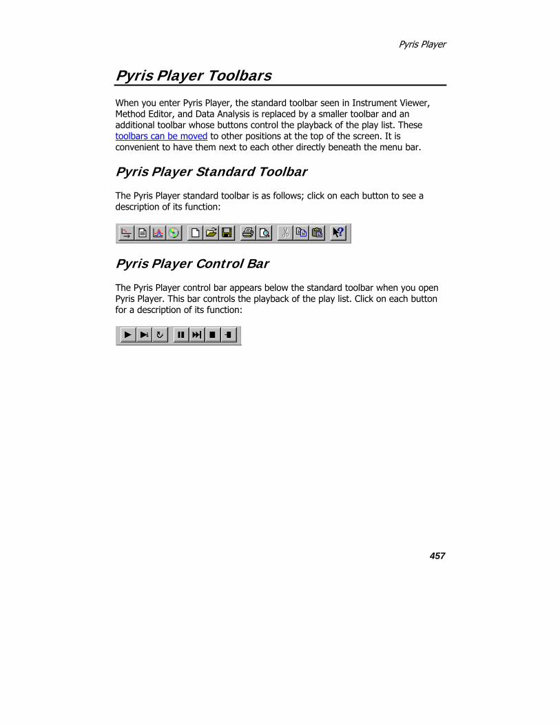
Pyris Player

457

Pyris Player Toolbars

When you enter Pyris Player, the standard toolbar seen in Instrument Viewer, Method Editor, and Data Analysis is replaced by a smaller toolbar and an additional toolbar whose buttons control the playback of the play list. These toolbars can be moved to other positions at the top of the screen. It is convenient to have them next to each other directly beneath the menu bar.

Pyris Player Standard Toolbar

The Pyris Player standard toolbar is as follows; click on each button to see a description of its function:

Pyris Player Control Bar

The Pyris Player control bar appears below the standard toolbar when you open Pyris Player. This bar controls the playback of the play list. Click on each button for a description of its function:

Pyris

458

Pyris Player Setup Page

If you select Pyris Player while in an Instrument Application, the Player opened is for that instrument alone. You can open Pyris Player from another Instrument Application for another instrument on your system. For example, if you have a Pyris 1 DSC with an autosampler and a DSC 7 Robotic System as your Thermal Analysis system, you can have a play list for each instrument operating simultaneously.

If you are in Data Analysis Application when you select Pyris Player, use the Setup page to select with which instrument you would like Player to be associated.

Analyzer Type

Note: Creation of Jade Pyris player playlists must be created in Instrument view ONLY.

Note: If you are running Pyris version 8 with a Jade DSC, all older play lists are compatible. However, play lists that you create for a Jade DSC application will not operate with a Pyris 6 DSC with software older than version 8.

If you are in the Data Analysis Application when you click on the Pyris Player button on the toolbar, then the drop-down list for Analyzer Type will display all available instruments from which to select the desired instrument. When you go to the Edit Play List page, the last play list displayed for that instrument is seen. If you are in an Instrument Application, the only instrument listed in the drop-down list is that particular instrument.

Lot ID

If your laboratory groups samples into lots, this field is where you can record the lot number of the samples you are going to run with the play list. This is particularly useful for runs on an autosampler.

Comment

You can enter free-form text describing what the playlist does in the Comment field. There is no limit to how long the comment can be.

Pyris Player

459

Pyris Player Edit Play List Page

The Edit Play List page is where you can create and save play lists or open existing lists to edit or run. The Player Steps area shows the steps of the list as you add, insert, or delete steps using the buttons to the right. The area underneath the Player Steps area, the Edit Step area, contains fields in which you enter values to be used in the play list. Enter the values and then click on the step in the list in order for the new values to be displayed in the Player Steps area. There are four main levels in a play list: Prepare Sample, Sample Group, File Group, and Data Analysis. These main levels contain second-level entries. Your play list does not have to have all four. A typical play list may contain a Prepare Sample section and a Data Analysis section. Another list may be just Data Analysis procedures.

Sample Group is used to run several samples with the same method. A Sample Group comprises a Sample List and a Data Analysis list. The samples in a Sample List are similar and are run using the same method. The data are then analyzed using the same data analysis commands. Sample Groups are particularly useful with an autosampler.

File Group can be used to analyze groups of data after they were collected. File Group comprises a File List and Data Analysis List. The File List contains one or more File List Items. The Data Analysis List contains zero or more data analysis items. File Group is designed in much the same way that Sample Group is designed. A major difference is in the File List as compared with the Sample List. A Sample List contains, in addition to the list of sample items, method information that is used to run each of the sample items in the list. A File List contains only the list of File items.

The Edit Play List page contains the following items: Player Steps box

Displays the steps of the play list as you add, insert, or delete them using the buttons to the right. The play list is initially displayed in expanded mode as it is created. You can compress parts of the play list by clicking on the minus signs next to the main-level items Prepare Sample, Sample Group, File Group, and Data Analysis. The second-level steps beneath will disappear and the minus sign will be replaced by a plus sign. You can see the play list alone and in its own window by clicking on the View Play List tab.

Pyris

460

Add a step button

Use this button to start creating a play list or to add a step to the end of an existing play list. The Player Step Options dialog box is displayed when you click on Add a step. The items available to add to an existing play list will depend on the type of analyzer and what is already in the play list. A play list always starts out with either Prepare Sample, Sample Group, File Group or Data Analysis. Insert a step button

As soon as one step is in the Player Steps area, the Insert a step button becomes selectable. When you insert a step, it appears above the step that was highlighted when you selected Insert a step. The items that appear in the

Pyris Player

461

Player Step Options dialog box for insertion depend on the main-level item immediately above the insertion point. Delete this step button

Highlight the step you want to remove from the play list and click on Delete this step. If other steps in the play list are dependent on this step, a Dependencies List dialog box is displayed. For example, if you try to delete a Display Curve step, you may be reminded that an Add Curve step below it depends on that step. Edit Step Section

Whenever an item is added or inserted into the play list, an item-sensitive Edit Step section appears below the Player Steps section. The step number and item name are shown. Parameters specific to the play list item are displayed for editing.

Pyris

462

Pyris Player View Play List Page

The Pyris Player View Play List page shows the current play list only. This view is useful for displaying the play list in compressed or expanded form. Since there are no buttons or an Edit Step area, the play list has more room for display. This makes it easier to read and to get a better overview of what the play list is doing. Use the “+” and the “–“ symbols to the left of the first-level items (numbered 1, 2, 3, etc.) to expand or compress the list beneath that item. Prepare Sample, Sample Group, File Group, and Data Analysis are like folders that contain additional folders and/or steps.

Pyris Player

463

Pyris Player View History Page

The View History page of Pyris Player lists the history of the playback of the play list. It is also a real-time update list so as a play list is in playback mode, the history list is dynamically revised to reflect the status of a play list step. There is a history entry, indicated by the symbol , for each time the play list is run, with the date and time of the run displayed. Click on the “+” to the left of History entry to “open up” the history folder; this displays the main-level entries of the play list: Prepare Sample, Sample Group, File Group, and Data Analysis. Click on the “+” next to those entries to open the folders and display the second-level steps in the folders. If there is a green checkmark before the step, the operation was performed successfully. If appears in front of a step, the operation failed. Double click on the “+” to the left of the to display an additional Error line that explains why the playback of the play list entry failed. A blue down arrow indicates that the step was skipped. A Pause is indicated by a blue flag .

Pyris

464

More Detail

Click on this button with a history entry highlighted to display a dialog box showing the date and the time that the entry was executed. Some entries' More Detail dialog boxes will contain additional information. For example, for a Start Method entry, the following dialog box is seen:

Delete History

Pyris Player

465

You can delete a history entry by clicking on this button. The focused line must be a History line when you select this feature. You are warned that the entire block, i.e., all the entries associated with that run, will be deleted. You can cancel the deletion request by clicking on the Cancel button. Delete All

This button will delete all of the history entries in the View History page. You are warned that the entire History List will be deleted and are given the chance to cancel the request. Expand All/Collapse All

These buttons toggle the display of the History List between full view and collapsed view. The sample History List above is expanded; all entries for all History files are displayed. The same History List collapsed is as follows:

Top

Pyris

466

DSC Autosampler Control Dialog Box

The Autosampler Control dialog box is displayed when you click on the

Autosampler Control button on the Pyris 1 DSC or the DSC 7 control panel. Use this dialog box to control the autosampler when there is an error and you need to access the autosampler or when you want to run an individual sample. Through this dialog box you can move samples to and from the sample tray and open and close the sample holder cover (Pyris 1 DSC only).

Since you control the autosampler, you must be aware if a sample pan is already in the sample holder when you select Load Sample from Location in the

Pyris Player

467

dialog box. The autosampler will not check for the presence of a sample pan before loading the pan from a specified carousel location. The Autosampler Control dialog box is the same for both instruments except that for a DSC 7 Robotics System, you cannot load or unload a reference pan and open and close the sample holder cover from the dialog box. You must perform these functions from the DSC 7 Robotics System keypad.

Change Sample Pan Select Carousel Location

Enter the location in the tray that will be used when you click on one of the three buttons used to change the location of the sample pan: load, unload, and move. Load Sample from Location

Commands the autosampler to load the sample pan in the selected location into the sample holder. The sequence of steps to load a sample in the DSC 7 Robotic System is different than that for the Pyris 1 DSC Autosampler. Unload Sample to Location

Commands the autosampler to remove the sample pan in the sample holder and place it back into the tray at the selected location. The sequence of steps to unload a sample from the DSC 7 RS is different than that for the Pyris 1 DSC Autosampler. Move Carousel to Location

Commands the sample tray to rotate so that the magazine containing the specified location faces the front of the instrument. Now the magazine changing tool can be inserted to remove the magazine.

Change Reference Pan (Pyris 1 DSC only) Select Carousel Location

Enter the location in the tray that will be used when you click on one of the two buttons used to change the location of the reference pan: load or unload. Load Reference from Location

Commands the Pyris 1 DSC autosampler to load the reference pan in the selected tray location into the reference sample holder. The sequence of steps is exactly the same as that for loading a sample. Unload Reference to Location

Pyris

468

Commands the Pyris 1 DSC autosampler to remove the reference pan in the reference sample holder and place it back into the tray at the selected location. The sequence of steps is the same as that for unloading a sample except that it does check for the presence of a pan in the selected location before starting.

Cover Control (Pyris 1 DSC only) Open Cover

Opens the sample holder cover. Close Cover

Closes the sample holder cover. Close

Closes the dialog box.

Pyris Player

469

Creating and Editing a Play List

When creating a play list for any analyzer, the items in the Player Step Options dialog box consists of Prepare Sample, Data Analysis, and Sample Group. The list of items in the Player Step Options dialog box when adding a line to or inserting a line into the play list depends on analyzer and the focused step at the time.

When you click on Add a step, the new step is always appended to the end of the play list, no matter which play list item is highlighted. When you click on Insert a step, the new step is inserted above the focused step. The choices displayed in the Player Step Options dialog box depend on what main-level item the added or inserted item will appear beneath: Prepare Sample, Data Analysis, or Sample Group. If you are adding or inserting a line beneath a Display Curve entry, which would appear under Data Analysis, the Player Step Options dialog box contains the same selections that appear in the Math, Calc, and Display menus.

The main-level items in a regular play list are numbered 1, 2, 3, etc. The second-level items are numbered x.1, x.2, x.3, etc., where x is the number of the main level item directly above. These items are indented. Dotted lines connect the main-level items to their second-level items. Since the area in which a play list's steps is small in the Edit Play List page, you can see more of the list in the View Play List page. You can get a better picture of the structure of the play list. As you add or insert steps into the play list, the Edit Step area below the Player Steps box displays information and fields specific to that step.

Another main-level item for a play list is Sample Group. This is a special feature of a play list that is meant for analyzing samples using an autosampler. A Sample Group comprises a Sample List and a Data Analysis List. The steps that you would have to enter into a regular play list are added automatically when a Sample List is run. A Sample Group can be embedded within a regular play list or it can stand alone. A play list can contain many Sample Groups. A Sample Group can be used with an analyzer without an autosampler. Automatic Pause dialog boxes are displayed at the appropriate points by the program. You would then have to remove or load a sample.

Quick Help

Pyris

470

Edit Step: File

The Edit Step: File area is displayed when you click on Add a file at the File Group window or the File List window. It is also displayed when the focused line is a File line in a File List. The items in this area vary with the analyzer you are using. Displayed below are the Edit Step: File areas for Diamond TG/DTA.

Pyris Player

471

Data File Select Play List Item

A file that is generated during the running of the playlist by a playlist item that occurs before the current Display Curve item. The items that generate data files during a playlist are Start Method (which is in the context of a Run Sample item) and the Sample item in a Sample List (which is in the context of a Sample Group). When there is one or more of these items (Start Method or Sample in a Sample List), the Select Play List Item is enabled.

This radio button is enable when the following occur:

Pyris

472

Must have a Start Method (which is in the context of a Run Sample item) and the Sample item in a Sample List (which is in the context of a Sample Group).

In File Group, click on the Add a File button. Choose the desire file from the Browse dialog and OK.

‘Select Play List Item’ radio button and drop down list are enabled.

If there are more than one Start Method, it will appear in the drop down list

They are data files generated by running the Prepare Sample or Sample Group items. If this radio button is selected, the you must select the available data files from the drop down list. Select Existing File

This field is always enabled when a file that exists at the time the playlist is being edited. To select an existing data file, click in this radio button and both the File Name field and the Browse button will be enabled. Enter the file name in the File Name field or use the Browse button to find and select the file. The Directory field will display the drive and directory where the file resides. Use Current Run

A file that is part of a File Group loop or a Sample Group loop - "Use Current Run" - This is enable for Display Curve items that are part of a File Group Data Analysis List or a Sample Group Data Analysis List. To select the data file currently running, click in this radio button. When Data Analysis finishes analyzing the file, it will capture the next data file that is currently running. Select Curves to Display

The curve displayed in the Data Analysis window depends on the curve type selected from the drop down list. Display Options

Start at Time Zero - If this checkbox is selected, the first point of each separate recall segment will be designated time zero.

Display Endotherms Up - Select this checkbox to display an upward graph.

Weight % - To normalized weight, select ‘Subtracted Weight’ from Select Curve Display and select the Weight% checkbox. If this checkbox is selected, it will display the weight unit as a percentage and not as mg.

Pyris Player

473

Steps - Select this checkbox to have a data recall Temperature Program segments from the run.

Save Data As File Name

This field is for the name of the file in which the data collected from the run will be saved. You can enter the file name directly in this field or in the Browse dialog box. A default file name is used if you do not specify a file name. The default name is taken from the entry made in the Save Preferences page. You can also use incremental file names, e.g., if you enter File# in the File Name field, the data file saved is FileXXX, where XXX starts at 001 and is incremented each time the method is used. This feature is useful when creating a Sample List. If when running the play list it is found that a file name already exists, the system will add a date/time stamp at the end of the new file name to distinguish it from the existing file. Browse

If you want to select a directory other than the default (selected in the Save Preferences page) for storing the data file, click on the Browse button to display the Browse dialog box. Directory

This field displays the drive and directory in which the data are saved after the run. This value reflects the disk\directory chosen in the Browse dialog box. If you do not select a specific directory, the default will be displayed.

Buttons Add a file

This button displays the Browse dialog box which allows the you to search through the mapped network drive or on the hard drive for saved data files. Selected data files are added to the File List. Insert a file

This button displays the Browse dialog box which allows the you to search through the mapped network drive or on the hard drive for saved data files. The selected file is inserted above the highlight data file. Delete file item

Highlight the data file you want to remove from the File List and click on Delete file item.

Pyris

474

Top

Pyris Player

475

Edit Step: File Group

When you select File Group from the Player Step Options dialog box, the Player Steps area displays the default items of a File Group:

1: File Group:

1.1: File List:

1.2: Data Analysis List:

The Edit Step area, which consists of a Comment field and a large blank area, is empty. As soon as you begin to add data files to the File List, the data files are listed in the large blank area:

Pyris

476

Comment

Enter free-form text describing the sample group about to be created. The entry appears next to Sample Group in the Player Steps area. Note that the text does not wrap when it reaches the end of the Comment box but keeps scrolling to the left. Add a File

Brings up the Browser dialog and let the you select the existing play list files. As the you begin adding data files to the File List, the files are listed in the blank area below the Comment box and the Edit Step: File area is displayed area is

Pyris Player

477

automatically displayed. To return to the Edit Step: File Group display, click on the File Group line in the Play Steps area.

479

Remote Monitor

Pyris

480

Remote Monitor

A powerful feature of the Pyris Software for Windows is that it can expand to a broad network of users. You can monitor the real-time status of and stop a run on an analyzer on a remote computer via a network connection. In the remote computer’s Remote Access page in Preferences, the user must select the amount of access to his analyzer(s) that a remote user is allowed. You can open a Remote Monitor window for each analyzer configured on the remote computer. In order to use the Remote Monitor feature, the security permission bits must be transferred from the Pyris Application Add On button to the Pyris Main security button. This is done at installation by your PerkinElmer Instruments Service Engineer. Once installed, the Remote Monitor option appears in the Tools menu.

Remote Monitor is part of the Data Analysis application. There is one Remote Monitor window per Data Analysis application.

Starting the Remote Monitor

To start the Remote Monitor for a Pyris analyzer: 1. Open a Data Analysis Application

At your Pyris computer, open a Data Analysis application either by selecting Data Analysis from the Start Pyris Task menu, by clicking on the Data Analysis icon on the toolbar, or by selecting it from the Pyris Software for Windows group in the Programs menu displayed from the Start button. At the Open Data File dialog box select any data file in order to open the Data Analysis application.

2. Open the Remote Monitor

Click on the Remote Monitor command in the Tools menu. The Select PC dialog box is displayed.

3. Select a Computer to Monitor

With the PC tab selected, display the drop-down list of names of computers on the network that you can monitor. The first time you open the Remote Monitor, the name of only your computer is listed. This is the name you assigned when you installed Windows. Add a computer to the list by typing its name in the

Remote Monitor

481

Name field. The next time you open the Remote Monitor, the computer name you entered will be displayed in the drop-down list. After entering the PC, click on Connect.

4. Select an Instrument to Monitor

After you select a computer to monitor, select the Instrument tab. All Pyris analyzers configured on the selected computer are listed in the drop-down list. Select the analyzer you want to monitor, then click on OK. Only analyzers that are connected and running can be selected. Analyzers that are configured but not running are grayed out and cannot be selected.

Viewing the Instrument Monitor and Status Panel

After selecting and connecting to the remote analyzer that you want to monitor, the Status Panel for that analyzer appears and the Instrument Viewer displays the remote analyzer’s real-time curve. The Status Panel on your computer screen is exactly the same as what you see on the screen of the computer to which the monitored analyzer is attached. In addition, the Status Panel contains a Stop Run button at the left-hand side. If you have permission, you can stop a run on the remote analyzer by clicking on Stop Run. Permission is set in the Remote Access page of Preferences.

The Status Panel is dockable. The current values of several analyzer parameters, read from the analyzer, are displayed in the Status Panel. You can customize the Status Panel to display different parameters. Display in the Instrument Monitor

If Remote Monitor is activated when the monitored analyzer is running, the curve(s) displayed will include data starting from the beginning of the run.

If Remote Monitor is activated when the monitored analyzer is not running, the curve(s) displayed will include data only from the time the remote connection is made.

If Remote Monitor is already on when a run begins on the monitored analyzer, the data is cleared and data from the beginning of a run is displayed. Turning the Instrument Monitor and Status Panel Off

When both the Status Panel and the Instrument Monitor are on and then the Status Panel is toggled off, the remote connection is maintained. The Status Panel can be redisplayed by clicking on Status Panel in the View menu.

Pyris

482

When both the Status Panel and the Instrument Monitor are on and then the Instrument Monitor is toggled off, the remote connection is maintained. The Instrument Monitor can be redisplayed by clicking on Monitor in the View menu.

When the Status Panel is displayed and the Instrument Monitor is off and then the Status Panel is toggled off, the connection to the remote analyzer is lost. The connection can be reestablished by using Remote Monitor in the Tools menu.

When the Instrument Monitor is displayed and the Status Panel is off and the Instrument Monitor is toggled off, the connection to the remote analyzer is lost. The connection can be reestablished by using Remote Monitor in the Tools menu.

Stopping a Run in the Remote Monitor

Select the Stop Run button in the Remote Monitor Status Panel to stop the sample run you are monitoring. When you select this button, a confirmation message appears; select No if you change your mind and do not want to stop the run.

The Stop Run button may be inhibited by the permission setting on the PC that is running the analyzer. Permission is set in the Remote Access page in Preferences. Permission settings are (1) no access to the analyzer, (2) status monitoring only (no ability to stop a run remotely), and (3) status monitoring and ability to stop a run.

Top

Remote Monitor

483

Remote Monitor

A powerful feature of the Pyris Software for Windows is that it can expand to a broad network of users. You can monitor the real-time status of and stop a run on an analyzer on a remote computer via a network connection. In the remote computer’s Remote Access page in Preferences, the user must select the amount of access to his analyzer(s) that a remote user is allowed. You can open a Remote Monitor window for each analyzer configured on the remote computer. In order to use the Remote Monitor feature, the security permission bits must be transferred from the Pyris Application Add On button to the Pyris Main security button. This is done at installation by your PerkinElmer Instruments Service Engineer. Once installed, the Remote Monitor option appears in the Tools menu.

Remote Monitor is part of the Data Analysis application. There is one Remote Monitor window per Data Analysis application.

Starting the Remote Monitor

To start the Remote Monitor for a Pyris analyzer: 1. Open a Data Analysis Application

At your Pyris computer, open a Data Analysis application either by selecting Data Analysis from the Start Pyris Task menu, by clicking on the Data Analysis icon on the toolbar, or by selecting it from the Pyris Software for Windows group in the Programs menu displayed from the Start button. At the Open Data File dialog box select any data file in order to open the Data Analysis application.

2. Open the Remote Monitor

Click on the Remote Monitor command in the Tools menu. The Select PC dialog box is displayed.

3. Select a Computer to Monitor

With the PC tab selected, display the drop-down list of names of computers on the network that you can monitor. The first time you open the Remote Monitor, the name of only your computer is listed. This is the name you assigned when you installed Windows. Add a computer to the list by typing its name in the

Pyris

484

Name field. The next time you open the Remote Monitor, the computer name you entered will be displayed in the drop-down list. After entering the PC, click on Connect.

4. Select an Instrument to Monitor

After you select a computer to monitor, select the Instrument tab. All Pyris analyzers configured on the selected computer are listed in the drop-down list. Select the analyzer you want to monitor, then click on OK. Only analyzers that are connected and running can be selected. Analyzers that are configured but not running are grayed out and cannot be selected.

Viewing the Instrument Monitor and Status Panel

After selecting and connecting to the remote analyzer that you want to monitor, the Status Panel for that analyzer appears and the Instrument Viewer displays the remote analyzer’s real-time curve. The Status Panel on your computer screen is exactly the same as what you see on the screen of the computer to which the monitored analyzer is attached. In addition, the Status Panel contains a Stop Run button at the left-hand side. If you have permission, you can stop a run on the remote analyzer by clicking on Stop Run. Permission is set in the Remote Access page of Preferences.

The Status Panel is dockable. The current values of several analyzer parameters, read from the analyzer, are displayed in the Status Panel. You can customize the Status Panel to display different parameters. Display in the Instrument Monitor

If Remote Monitor is activated when the monitored analyzer is running, the curve(s) displayed will include data starting from the beginning of the run.

If Remote Monitor is activated when the monitored analyzer is not running, the curve(s) displayed will include data only from the time the remote connection is made.

If Remote Monitor is already on when a run begins on the monitored analyzer, the data is cleared and data from the beginning of a run is displayed. Turning the Instrument Monitor and Status Panel Off

When both the Status Panel and the Instrument Monitor are on and then the Status Panel is toggled off, the remote connection is maintained. The Status Panel can be redisplayed by clicking on Status Panel in the View menu.

Remote Monitor

485

When both the Status Panel and the Instrument Monitor are on and then the Instrument Monitor is toggled off, the remote connection is maintained. The Instrument Monitor can be redisplayed by clicking on Monitor in the View menu.

When the Status Panel is displayed and the Instrument Monitor is off and then the Status Panel is toggled off, the connection to the remote analyzer is lost. The connection can be reestablished by using Remote Monitor in the Tools menu.

When the Instrument Monitor is displayed and the Status Panel is off and the Instrument Monitor is toggled off, the connection to the remote analyzer is lost. The connection can be reestablished by using Remote Monitor in the Tools menu.

Stopping a Run in the Remote Monitor

Select the Stop Run button in the Remote Monitor Status Panel to stop the sample run you are monitoring. When you select this button, a confirmation message appears; select No if you change your mind and do not want to stop the run.

The Stop Run button may be inhibited by the permission setting on the PC that is running the analyzer. Permission is set in the Remote Access page in Preferences. Permission settings are (1) no access to the analyzer, (2) status monitoring only (no ability to stop a run remotely), and (3) status monitoring and ability to stop a run.

Top

487

Quick Help

Pyris

488

Explore the Software

How Do I Use the Pyris Manager?

How Do I Start the Software?

How Do I Configure My System?

How Do I Monitor System Status?

How Do I Perform Run?

Where Do I Look at Data?

How Do I Print?

How Do I Shut Down the System?

Quick Help

489

Calibrate an Analyzer

What would you like to do?

Calibrate a Pyris Diamond TG/DTA

Calibrate a Pyris Diamond DSC

Calibrate a Pyris 1 DSC Calibrate a DSC 7 Calibrate a Pyris 6 DSC Calibrate a TGA 7 Calibrate a Pyris 6 TGA Calibrate a Pyris 1 TGA Calibrate a DMA 7e Calibrate a TMA 7 Calibrate a DTA 7 Restore Calibration

Apply existing calibration file values:

When you open the Calibration window, the current calibration file's values are displayed. Suppose you are going to run some samples in a different temperature range than the one you have been using and that you calibrated the instrument for that range previously and saved the file. Select Open from the File menu, select the desired calibration file, click on Save and Apply to apply the calibration file's values to the analyzer, and click on Close.

Pyris

490

Prepare for Data Collection

Before performing a run on your samples, you need to set up a method which is a set of parameters that are used by the analyzer while collecting data. A method is set up by loading it into the Method Editor and editing the parameters, if necessary. The parameters in the method depend on the conditions used, the type of sample, the type of information you are looking for, and so on. Once the method is ready, you click on the Start Method button on the control panel and the run begins.


Create a New Method Select an Existing Method Run a Sample Using Baseline Subtraction

Quick Help

491

Performing Data Collection

Once you have set up the method to use for your run, you can begin data collection. The Hardware Help contains detailed instructions on how to perform runs for calibrating the analyzer. These instructions give you a good idea of what a routine run is like for that instrument. The sites below bring you into the Hardware Help for a look at how to run reference materials for each analyzer. Indium run for DMA 7e

Indium run for TMA 7

Indium and zinc runs for Pyris 6 DSC

Aluminum and gold runs for DTA 7

Other sites to visit for information on data collection are the sample preparation and sample loading topics for each analyzer.

Pyris

492

View Your Data


Look at Collected Data During a Run

Open a Data Analysis Window

Display a Curve

Open a Data File

Add a Data File to the Window

Select Steps to Display

Change the Active Curve

Display Results

Quick Help

493

Optimize Your Data


Rescale the X or Y Axis

Display the X Axis, Y Axis, or Both Axes at Full Scale

Use the Radar Window to Rescale a Curve

Shift a Curve

Change the Slope of a Curve

Pyris

494

Perform a DMA Analysis

This is a step-by-step outline for performing a DMA analysis:

Check purge gas, cooling device, and coolant.

Select and install a measuring system.

Tare the probe.

Zero the probe.

Select the type of test method and enter parameters in Method Editor.

Measure sample dimensions and mount the sample.

Start the run and calculate and plot results.

Quick Help

495

Perform a Purity Analysis

The following topics provide the steps for performing a Purity analysis of DSC data:

Prepare samples and data

Performing the Purity calculation

Reading the results

Prepare Samples and Data The preferred method of encapsulating DSC samples involves hermetically sealing the sample between two volatile sample pans or placing a thin disk of aluminum on top of the sample before sealing the pan. Items used for encapsulating DSC samples for Purity analysis include a Volatile Sample Sealer (P/N 0219-0061) and Volatile Sample Pans and Covers (P/N 0219-0062). The data for a Purity analysis must be from the melting of a fairly pure organic or inorganic material but not a polymer.

1. To prepare your data for Purity analysis, perform a sample run with your DSC 7, Pyris 6 DSC, or Pyris 1 DSC.

2. For best results, use a slow scanning rate (e.g., 1C/min or less) and use an average sample size (e.g., 1 – 3 mg). This should produce a peak height of approximately 2 – 10 mW.

3. Make sure that the X axis is Temperature not Time. Use Rescale X to change if necessary.

4. Click on the Data Analysis button on the toolbar to open the Data Analysis application for that analyzer on which the data were collected.

5. In the Open File dialog box select the data file from the run you just performed.

Performing the Purity Calculation With the data file from your Purity analysis run displayed in the Data Analysis window:

1. Select Purity from the Calc menu. The Calculate Peak Area dialog box is displayed and two X’s appear on the curve.

Pyris

496

2. Select left and right peak limits by either entering the values directly into the fields in the dialog box or by clicking on and dragging the X to the desired position on the curve.

3. Click on Next. The Select Calculation Method dialog box is seen next.

4. Select the Calculation Method: Standard or MLR.

5. Enter the thermal resistance constant R0 of the sample.

6. Enter the molecular weight of the sample.

7. Enter the heat capacity Cp of the sample pan.

8. Click on the Next button. If you selected the Standard method, the next screen is Adjust % Area Limits. If you selected the MLR method, you see Adjust Baseline.

9. If you must adjust the baseline for an MLR method, enter the limits into the fields or move the two X’s on the curve. Click on the Next button.

10. To adjust the % Area Limits, enter the limits directly into the fields in the dialog box or move the vertical red bars on the curve.

11. Click on the Next button. The View Curves dialog box is next.

12. To show how the data fits the Van’t Hoff relationship, select T vs 1/F by clicking in the check box.

13. Click on the Finish button.

The results of the calculation are displayed on the screen.

Reading the Results The results of a Purity analysis are as follows:

Limit 1 – lowest temperature used for the purity calculation Limit 2 – highest temperature used for the purity calculation Delta Hf – heat of fusion (kJ/mole) Tm – melting point of the displayed data T0 – melting point of theoretically pure sample X correction – correction for melting below Limit 1 Purity – percent of pure material in the displayed data The inputs are also displayed with the results: Method – standard or MLR X1 – left baseline limit X2 – right baseline limit R0 – thermal resistance constant of the sample pan

Quick Help

497

Molecular Weight – molecular weight of the sample material Cp (pan) – heat capacity of the sample pan In the T vs 1/F curve, the corrected data points are shown as red circles and the line drawn through them shows how the data fit the Van’t Hoff relationship. The blue boxes represent the uncorrected values calculated for 1/F (fraction melted) at given temperatures.

Pyris

498

Determine Lag or Rate Compensation

In thermal analysis, thermal lags affect the accuracy of the temperature of the scanning data. As a sample is heated or cooled, the heat flowing into it produces temperature gradients in the sample and the instrument. Therefore, it is recommended that for the highest temperature accuracy, the analyzer must be calibrated at the conditions to be used for the experiment, including the scan rate.

To determine the lag or scan rate compensation for a DSC:

1. Restore all calibration values to their default values by selecting Calibrate from the View menu and then Restore All from the Restore menu.

2. Set Lag Compensation to its default value of 0 by selecting the DSC 7 or Pyris page in Preferences (on the Tools menu) and entering 0 in the Lag Compensation field. Record the current lag compensation value so you can return your system to its current state if necessary.

3. Click on OK to save your entry and exit Preferences.

4. Prepare an indium sample of weight 5.0 + 0.5 mg and place in a sample pan that you plan to use for routine operation of your analyzer.

5. Perform heating scans on the indium sample using the following parameters:

• Purge gas = gas you use for routine operation

• Start temperature = 120C

• End temperature = 170C

• Scan rates = 5C/min and 20C/min

• Load temperature = 50C

Be sure to cool to the Load temperature after the first indium scan and hold the temperature there for at least 5 minutes prior to starting the second indium scan.

6. Perform a Peak Area calculation on each indium melting scan.

7. Perform the following calculation to determine the lag compensation value for your analyzer:

Lag Comp. = (T1 – T2) / (R1 – R2)

Quick Help

499

where T1 is peak onset temperature for the 20C/min scan T2 is peak onset temperature for the 5C/min scan R1 is 20C/min R2 is 5C/min

8. Multiply the lag compensation value just calculated by 1000 and enter that value in the DSC 7 or Pyris page in Preferences.

9. Click on OK to save the Lag Compensation value and exit Preferences.

10. Recalibrate the analyzer using the calibration procedures described in Calibration of the DSC.

After determining the lag compensation, this value will be applied automatically to all future experiments until you change the value in Preferences.

Pyris

500

Display Curve Data in Third-Party Software

To display the data of a specific curve in Microsoft Excel:

1. Display or focus (highlight by clicking on) the curve of interest in the Data Analysis application.

2. From the Edit menu, select Copy.

3. Switch to the Excel application.

Notice the heavy black outline around the first cell in the upper-left-hand corner of the spreadsheet. Leave the outline on the box.

4. Select Paste from the Edit menu.

5. From the Format menu, select Column and then Autofit Selection.

6. Unhighlight the data and scroll down the spreadsheet to review the data, deleting any unwanted rows.

To display a curve’s data in Word for Windows:

1. Display or focus the curve of interest in the Data Analysis application.

2. From the Edit menu select Copy.

3. Switch to Word for Windows.

4. Select Paste from the Edit menu.

5. Highlight the two columns of numbers.

6. Select Convert Text to Table from the Table menu.

7. In the dialog box, choose Tabs for Separate Text At and 2 for the Number of Columns; click on OK.

8. With the columns still highlighted, go to Cell Height and Width in the Table menu and adjust the width of the columns as necessary.

9. Place the cursor outside of the table and click to unhighlight the data. Then scroll down the table to review, deleting any unwanted rows.

Quick Help

501

Display Entire Data File in Third Party Software

To display all data of a data file in Microsoft Excel:

1. Open the data file in the Data Analysis application.

2. Click on the Method Used button in the toolbar.

3. Click on the Create button. The Create Data File dialog box is displayed.

4. Select Include Data Points.

5. Record the path to which the .TXT file is to be saved and click on OK.

6. Click on the OK button to return to the Data Analysis window.

7. Switch to the Excel application.

Notice the heavy black outline around the first cell in the upper-left-hand corner of the spreadsheet. Leave the outline on the box.

8. Select Open from the File menu.

9. In the Open dialog box, display the drop-down menu under List Files of Type and select Text File.

10. Follow the path recorded in step 5 and find the file that was created in Pyris; highlight it and click on OK.

11. The Text Import Wizard box is displayed next. The responses to be entered to this wizard and subsequent screens are as follows (these are the default entries):

Delimited | Next | Tab | Next | General | Finish

12. Click on the blank button that is next to the “A” column header and above the numbered row column. This will highlight the entire document.

13. From the Format menu, select Column and AutoFit Selection.

14. Unhighlight the table and scroll down to review the data, deleting any unwanted rows.

To display all of a data file’s data in Word for Windows:

1. Open the data file in the Data Analysis application.

2. Click on the Method Used button in the toolbar.

Pyris

502

3. Click on the Create button. A dialog box is displayed.

4. Select Include Data Points.

5. Record the path to which the .TXT file is to be saved and click on OK.

6. Click on the OK button in the Options page to return to the Data Analysis window.

7. Switch to Word for Windows.

8. Select Open from the File menu.

9. In the Open dialog box, display the drop-down menu under List Files of Type and select Text File.

10. Follow the path recorded in step 5 and find the file that was created in Pyris; highlight it and click on OK.

11. Highlight the two columns of numbers.

12. In the Table menu select Convert Text to Table.

13. In the dialog box, choose Tabs for Separate Text At and 2 for the Number of Columns; click on OK.

14. With the columns still highlighted, go to Cell Height and Width in the Table menu and adjust the width of the columns as necessary.

15. Place the cursor outside of the table and click to unhighlight the data. Then scroll down the table to review the data, deleting any unwanted rows.

Quick Help

503

Create a Play List

We give four examples of creating play lists: two for nonautosampler analyzers which contain commands for analyzing a data file, and two for analyzers with an autosampler. These are fairly simple play lists but they will give you an idea of the power and flexibility of play lists.

Pyris 6 TGA Play List

Pyris 1 DSC Play List

Pyris 1 DSC with Autosampler Play List

Pyris 1 TGA with Autosampler Play List

505

Applications

Pyris

506

DMA Applications

DMA Applications

The following list is a good cross section of the types of applications for which you can use your DMA 7e:

Glass Transition Analysis of Epoxy–Glass Composite Using DMA

Fast Mechanical Characterization of an Epoxy Composite

Isothermal Cure of an Epoxy by DMA

Softening Temperature Determination Using the DMA 7e

DMA 7e Modulus Reported by Each Measuring System

DMA 7e Flexural Modulus Determination

DMA 7e Compressive Modulus Determination

DMA 7e Tensile Modulus Determination

PID Factors for Position Control

Isothermal Modulus Determination Using Position Control

Thermal Characterization of a Thin Film Using Position Control

Glass Transition Analysis of Epoxy–Glass Composite Using DMA

Introduction

At temperatures below the glass transition (Tg), a composite behaves like a glassy material. At higher temperatures, the composite behaves like a viscoelastic material.

Applications

507

Theory

The glass transition is often used to identify the temperature range of the glassy to viscoelastic transition.

Instrument

Use the DMA 7e Dynamic Mechanical Analyzer equipped with the stainless-steel 3-point bending measuring system with a 20-mm bending platform and a 10-mm knife edge.

Sample Preparation

Cut a sample that measures 23 mm long by 3 mm deep. Using tweezers, place the sample directly on the 3-point bending platform. No further sample preparation or clamping is necessary.

Method

Program the temperature scan from 50°C to 225°C at a heating rate of 2°C/min. A typical method is as follows:

Sample: Epoxy-Glass Composite

Instrumental: Analyzer: DMA 7e Measuring System: 3-Point Bending Geometry: Rectangle

Environmental: Purge: Nitrogen Coolant: Ice water

Parameters: Method: Temperature Scan Static Force: 550 mN Dynamic Force: 500 mN Frequency: 1 Hz Heat from 50°C to 225°C at 2°C/min

Controls: Static Force Dynamic Force

Pyris

508

Results/Discussion

The figure above shows a plot of storage modulus and tangent delta versus temperature. The change in the curves indicates the glass transition region in the 120°C – 175°C range. The onset of softening of the storage modulus (i.e., indicative of the material storing energy) occurs at approximately 125°C; the peak of tan delta occurs at approximately 136°C.

A decrease in the storage modulus at approximately 120°C indicates a decrease in the stiffness of the composite. The decrease occurs because the composite softens from its glassy state, a state dominated by the resin and fiber composite structure. At higher temperatures, the storage modulus finally reaches a minimum value as the contribution from the resin decreases and the contribution from the fiber increases.

The methodology outlined in this application example can be applied to a wide variety of thermosets, thermoplastics, and composites. No special sample

Applications

509

preparation is necessary. Further analysis includes parallel plate analysis for the neat resin to determine the gel point or characterize cure. Additional testing may include examination of the beta and gamma transitions as well as frequency dependence. Also, TGA can be used to evaluate the moisture content or the effect of the outgassing that occurs at these temperatures while DSC can be used to confirm the thermal transitions.

References

Brennan, W.P., Cassel, R.B., “Applications of Thermal Analysis in the Electrical and Electronics Industries,” Thermal Analysis Applications Study No. 25. The Perkin-Elmer Corporation, Norwalk, CT, 1978.

Cassel, R.B., “Characterization of Thermosets,” Thermal Analysis Application Study No. 19. The Perkin-Elmer Corporation, Norwalk, CT, 1977.

Gray, A.P., “Establishing a Correlation Between the Degree of Cure and the Glass Transition Temperature of Epoxy Resins,” Thermal Analysis Applications Study No. 2. The Perkin-Elmer Corporation, Norwalk, CT, 1972.

Top

Fast Mechanical Characterization of an Epoxy Composite

Introduction

Storage modulus has been widely accepted as a tool to characterize performance and processability of composites. The storage modulus has also been used to characterize impact properties, dimensional stability (warpage), the degree of cure, effects of modifiers, tougheners, extenders, fire retardants, and other additives.

Theory

Examination of a material’s modulus at room temperature is a deceptively simple and effective test that can yield useful information about a composite.

Pyris

510

Instrument

Use the DMA 7e Dynamic Mechanical Analyzer equipped with the stainless-steel 3-point bending measuring system with a 15-mm bending platform and a 10-mm knife edge.

Sample Preparation

Cut a sample measuring approximately 23 mm long by 3 mm deep. Using tweezers, place it directly on the 3-point bending platform. No further sample preparation or clamping is necessary.

Method

Program an isothermal scan at 25°C for 3 min. A typical method is as follows:


Instrumental: Analyzer: DMA 7e Measuring System: 3-Point Bending Geometry: Rectangle Sample height (y): 0.865 mm Sample width (x): 15.000 mm Sample depth (z): 3.016 mm

Environmental: Purge: Nitrogen (30 cc/min) Coolant: Ice water

Parameters: Method: 1-min Isothermal Scan Static Force: 550 mN Dynamic Force: 500 mN Frequency: 1 Hz

Controls: Static: Force Dynamic: Force Temperature: 25°C

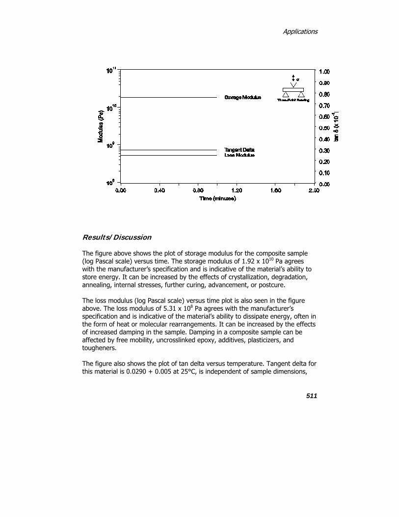
Applications

511

Results/Discussion

The figure above shows the plot of storage modulus for the composite sample (log Pascal scale) versus time. The storage modulus of 1.92 x 1010 Pa agrees with the manufacturer’s specification and is indicative of the material’s ability to store energy. It can be increased by the effects of crystallization, degradation, annealing, internal stresses, further curing, advancement, or postcure.

The loss modulus (log Pascal scale) versus time plot is also seen in the figure above. The loss modulus of 5.31 x 108 Pa agrees with the manufacturer’s specification and is indicative of the material’s ability to dissipate energy, often in the form of heat or molecular rearrangements. It can be increased by the effects of increased damping in the sample. Damping in a composite sample can be affected by free mobility, uncrosslinked epoxy, additives, plasticizers, and tougheners.

The figure also shows the plot of tan delta versus temperature. Tangent delta for this material is 0.0290 + 0.005 at 25°C, is independent of sample dimensions,

Pyris

512

and is indicative of the properties of a composite. It is not necessary to measure the sample and enter sample dimensions if this is the only curve to be analyzed.

The methodology outlined in this application example can be applied to a wide variety of thermosets, thermoplastics, and composites. No special sample preparation is necessary. Parallel plate analysis of the neat resin for determining the gel point or for characterizing cure can also be performed. Additional testing includes examination of the beta and gamma transitions as well as frequency dependence. TGA can be used to evaluate the moisture content or effect of outgassing that occurs at these temperatures while DSC can be used to confirm the thermal transitions.

References

Brennan, W.P., Cassel, R.B., “Applications of Thermal Analysis in the Electrical and Electronics Industries,” Thermal Analysis Applications Study No. 25. The Perkin-Elmer Corporation, Norwalk, CT, 1978.

Cassel, R.B., “Characterization of Thermosets,” Thermal Analysis Application Study No. 19. The Perkin-Elmer Corporation, Norwalk, CT, 1977.

Gray, A.P., “Establishing a Correlation Between the Degree of Cure and the Glass Transition Temperature of Epoxy Resins,” Thermal Analysis Applications Study No. 2. The Perkin-Elmer Corporation, Norwalk, CT, 1972.

Top

Softening Temperature Determination Using the DMA 7e

Introduction

The DMA 7e method described here is optimized for performing vicat softening temperature determinations for a broad range of thermoplastics, elastomers, and some thermosets in the rigid and semirigid states. Samples in the form of disks or rectangles are mounted using the 1-mm parallel plate (compression) measuring system. The softening temperature is the temperature at which a 1-mm probe penetrates 1 mm into the sample. This measurement is made while the sample is heated and a 5000-mN force is applied.

Applications

513

NOTE: The instrument can be modified to accommodate an oil bath, but good temperature precision is obtained using the standard furnace system. Temperatures can be verified using primary melting standards. A force of 500 gF (gram force) was used in this test. A force of 1000 gF can be achieved using weights in the weight tray.

Theory

Softening temperature determinations provide a qualitative measure of the temperature resistance of a material. Standard test methods have been created by ASTM and ISO to define the vicat softening temperature determination (1–3).

Instrument

Use the DMA 7e Dynamic Mechanical Analyzer equipped with the stainless-steel parallel plate measuring system with a 1-mm plate probe tip.

Sample Preparation

Cut the sample, an injection-molded 2-mm-thick sheet of styrene-butadiene, into disks using a heavy-duty 6-mm hole punch. Tare the weight and zero the height. Mount the sample by placing two disks on the bottom plate, lowering the probe, and visually aligning it with the top plate.

Method

Program the temperature scan from 30°C to 250°C at 2°C/min (120°C/h). Use a faster heating rate if all the samples are exposed to the same temperatures and the temperature is controlled to within + 1°C. Enter a static force of 5000 mN (6.37 x 106 Pa), a dynamic force of 10 mN (1.27 x 104 Pa), and a frequency of 10 Hz in the Initial State page. The dynamic force and frequency are included to enhance probe position sensitivity. Raise the furnace and allow the sample, analyzer, and furnace to equilibrate for about 2 min or until the probe position stabilizes. Read the sample height and start the run. When the probe has penetrated more than 1 mm, stop the run by pressing the Probe Up button on the analyzer.

A typical method for this application is as follows:

Pyris

514

Sample: Styrene Butadiene

Instrumental: Analyzer: DMA 7e Measuring System: 1-mm Parallel Plate Geometry: Disk Sample Height (y): 4.054 mm Sample Diameter (d): 1 mm

Environmental: Purge Gas: Nitrogen (20 cc/min) Coolant: Tap Water

Parameters: Method: Temperature Scan Static Force: 5000 mN Dynamic Force: 10 mN Frequency: 10 Hz Heat from 30°C to 250°C at 2°C/min

Applications

515

Results/Discussion

The figure above is a plot of probe position (linear millimeter scale) versus temperature for the SBR sample. There is a decrease in the probe position resulting from the slow penetration of the probe as the sample is heated and the stress placed upon it. Above 50°C, the probe position begins to decrease rapidly as the sample approaches its melting temperature. A few degrees above 80°C the sample melts and the probe position indicates 0 mm.

Perform an onset calculation on the probe position curve. Place the left tangent on the original sample height at 30°C and the right tangent on the midpoint of melting, and include a trigger value in the calculation. The onset of the melt and the softening temperature of this sample occur at 84.07°C. The 1-mm trigger is reported as 86.18°C.

References

“Standard Test Methods for Vicat Softening Temperature of Plastics” ASTM Standard D1525-91, Annual Book of ASTM Standards. ASTM, Philadelphia, 1994, Vol. 08.01.

“Vicat Softening Temperature of Thermoplastics,” ISO 306; ISO Standards Handbook 21 - Plastics. ISO, Geneva, 1990, Vol. 2.

“Vicat Softening Temperature of Unplasticized PVC Pipes and Fittings,” ISO 2507; ISO Standards Handbook 21 - Plastics. ISO, Geneva, 1990, Vol. 3.

DMA 7e Modulus Reported by Each Measuring System

Introduction

The DMA 7e measuring systems, combined with the many sample geometries available, provide an unequaled versatility in modulus determination. The measuring systems allow you to determine the modulus of samples in various physical states from viscous liquids to melts, semisolids, solid bars, films, and fibers. The modulus obtained by each measuring system is identified by its own symbol, as shown in the table below. Standard terminology has been established in the literature and by ASTM and ISO that defines the moduli reported by DMA measuring systems (1–9).

Pyris

516

Each measuring system applies stresses differently resulting in a different displacement of the sample and, thus, the calculation of a different type of modulus. The modulus obtained from one geometry may not relate to that obtained by another geometry.

Theory

A modulus is defined as the stress divided by the sample strain. Modulus is typically determined within the linear region (or elastic limit) of the test material. This region can be defined by finding the first region where the modulus curve approaches linearity, making certain that there are no anomalies in the stress vs. strain curve.

Instrument

Use the DMA 7e Dynamic Mechanical Analyzer to determine modulus.

Discussion

The DMA 7e consists of measuring systems used to determine different moduli. The table below lists the types of moduli and the measuring systems used to determine them. Flexural modulus (E) is determined by using a flexural deformation that is composed of compression on the top of the sample, tension on the bottom side of the sample, and gradient shear through the center of the sample. Tensile modulus (M) is determined by using uniaxial, unidirectional tensile deformation. Shear modulus (G) is ideally determined by using a cubical element in simple shear. Here, shear modulus is approximated by using flexural, tensile, or compressive deformations and applying Poisson's ratio. For example, a flexural modulus of 9 x 109 Pa gives a shear approximation of 3x109 Pa. Bulk (compressive) modulus (K) is determined by using bulk volumetric (dilatometer) deformations. Compressive modulus (L) is determined by using a uniaxial, (longitudinal) unidirectional compressive deformation.

Type of Modulus Symbol Sample Geometry Measuring System Part Number

Flexural E Bar or rod 3-Point Bending Standard

Flexural E Bar or rod 4-Point Bending Standard

Flexural E Bar or rod Dual Cantilever N539-0131

Applications

517

Flexural E Bar or rod Single Cantilever N539-0131

Flexural E Bar or rod 3-Point Bending N539-0136

Tensile M Film Extension N539-0132

Tensile M Fiber Extension N539-0132

Tensile M Film Quartz Extension N539-0134

Tensile M Fiber Quartz Extension N539-0134

Bulk K Volumetric Dilatometer N539-0763

Shear G Flowing Shear Standard

Compressive L Disk or rectangle Parallel Plates N539-0133

Compressive L Disk or rectangle Cup and Plates N539-0464

Compressive L Disk or rectangle Plate and Tray N539-0469

Compressive L Disk or rectangle Sintered Plates N539-0460

Compressive L Disk or rectangle Quartz plates N539-0135

References

“Standard Terminology Relating to Dynamic Mechanical Measurements on Plastics,” ASTM Standard D4092-90, Annual Book of ASTM Standards. ASTM, Philadelphia, 1994, Vol. 08.02.

“Terminology and Symbols,” ISO Standards Handbook 21 - Plastics. ISO, Geneva, 1990, Vol. 2.

“Standard Terminology Relating to Plastics,” ASTM Standard D883-93, Annual Book of ASTM Standards. ASTM, Philadelphia, 1994, Vol. 08.01.

Pyris

518

“Standard Terminology Relating to Methods of Mechanical Testing,” ASTM Standard E6-91, Annual Book of ASTM Standards. ASTM, Philadelphia, 1994, Vol. 03.01.

“Standard Practice for Rheological Measurement of Polymer Melts Using Dynamic Mechanical Procedures,” ASTM Standard D4440-93, Annual Book of ASTM Standards. ASTM, Philadelphia, 1994, Vol. 08.03.

“Standard Practice for Determining and Reporting Dynamic Mechanical Properties of Plastics,” ASTM Standard D4065-93, Annual Book of ASTM Standards. ASTM, Philadelphia, 1994, Vol. 08.02.

“Definitions,” ISO 472, ISO Standards Handbook 21 - Plastics. ISO, Geneva, 1990, Vol. 1.

Neilsen, L.E., Mechanical Properties of Polymers and Composites (in two volumes); Marcel Dekker, New York, 1974.

Ferry, J.D., Viscoelastic Properties of Polymers. Wiley & Sons, New York, 1970.

DMA 7e Flexural Modulus Determination

Introduction

The DMA 7e method described here is optimized to perform flexural modulus determinations for a broad range of materials including thermosets, thermoplastics, elastomers, and samples that are reinforced, nonreinforced, impact-modified, or filled and in the solid and the semisolid states. In flexural modulus determinations, samples in the form of rectangular bars or cylindrical rods are mounted using the three-point bending (flexural) measuring system. (Four-point bending, single- and dual-cantilever systems also may be used.)

Theory

Standard test methods have been created by ASTM and ISO to define the flexural modulus determination (1,2). Flexural modulus (E) is a measure of the resistance of the sample to flexural deformation and can be used as an indicator of stiffness or rigidity. Flexural deformation that is composed of compression on the top of the sample, tension on the bottom of the sample, and gradient shear through the center of the sample. Flexural modulus is similar to but does not necessarily equate to Young's modulus of elasticity.

Applications

519

Instrument

Use the DMA 7e Dynamic Mechanical Analyzer equipped with the stainless-steel 3-point bending measuring system with a 20-mm bending platform and a cylindrical knife edge.

Sample Preparation

With the micrometer measure and cut the sample, in this case a commercial grade bisphenol-A-type epoxy resin composite with four layers of E-type woven glass reinforcement, to the following dimensions: approximately 1 + 0.5 mm high by 23 + 3 mm wide by 3 + 1 mm deep. Cut the sample uniformly to prevent glass fiber splinters, shattered resin, or burrs.

Method

Program a static stress scan at 25°C for 3 min (see the rest of the parameters of the method below). Mount the sample on the bending platform and visually align it. Before starting the run, allow the furnace to equilibrate at 23°C for about 2 min or until the probe position stabilizes. Hold the sample in place initially with a minimal static stress, then increase the static stress. Use the response of the sample (static strain) to calculate the static flexural modulus.

NOTE: The flexural modulus is determined in the linear region of stress and strain. The proportional limit, yield, drawing, ultimate strength, and other results can be determined using other methods

Sample: Epoxy-Glass Composite: Rectangular bar

Instrumental: Analyzer: DMA 7e Measuring System: Three Point Bending Geometry: Rectangle Sample Height: 1.096 mm Sample Width: 20.000 mm Sample Depth: 2.991 mm

Environmental: Purge Gas: Helium (20 cc/min) Coolant: Tap Water

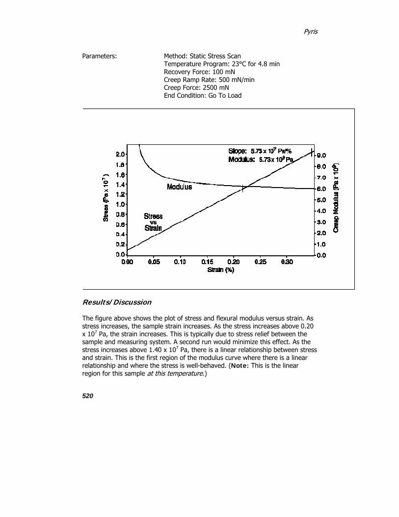
Pyris

520

Parameters: Method: Static Stress Scan Temperature Program: 23°C for 4.8 min Recovery Force: 100 mN Creep Ramp Rate: 500 mN/min Creep Force: 2500 mN End Condition: Go To Load

Results/Discussion

The figure above shows the plot of stress and flexural modulus versus strain. As stress increases, the sample strain increases. As the stress increases above 0.20 x 107 Pa, the strain increases. This is typically due to stress relief between the sample and measuring system. A second run would minimize this effect. As the stress increases above 1.40 x 107 Pa, there is a linear relationship between stress and strain. This is the first region of the modulus curve where there is a linear relationship and where the stress is well-behaved. (Note: This is the linear region for this sample at this temperature.)

Applications

521

Above a stress of 2.00 x 107 Pa, the system produces an increasing and nonproportional strain as the linear region is exceeded and the proportional limit is reached. This is a result of the sample sliding over the platform knives, alignment, end effects, and edge effects.

The flexural modulus (E) is defined as the slope of the flexural stress versus the flexural strain in the linear region. The slope of the stress/strain curve in this region is 5.73 x 107 Pa/%. This is multiplied by 100 to cancel the unit of % strain, yielding a flexural modulus of 5.73 x 109 Pa in the linear region for this sample at 23°C.

The Pyris software can also calculate the flexural modulus and present it as a curve as seen in the figure above. Above a stress of 1.40 x 107 Pa, the flexural modulus is approximately 5.73 x 109 Pa.

References

“Standard Test Methods for Flexural Properties of Unreinforced and Reinforced Plastics and Electrical Insulating Materials [Metric],” ASTM Standard D790M-92, Annual Book of ASTM Standards. ASTM, Philadelphia, Vol. 08.01.

“Determination of Flexural Properties of Rigid Plastics,” ISO 178, ISO Standards Handbook 21 - Plastics. ISO, Geneva, 1990, Vol. 1.

DMA 7e Compressive Modulus Determination

Introduction

This DMA 7e method is optimized to perform compressive modulus determinations for a broad range of materials including thermosets, thermoplastics, elastomers and samples that are vulcanized, unvulcanized, cured, modified, extended, or filled, in the solid and semi-solid state.

In compressive modulus, determination, samples can be mounted in the form of rectangles or cylindrical disks using the parallel plate (compressive) measuring system.

Theory

Standard test methods have been created by ASTM and ISO to define the compressive modulus determination (1,2). Compressive modulus (L) is a measure of the resistance of the sample to compression and is an indicator of

Pyris

522

stiffness or rigidity. Compressive modulus is determined by using a uniaxial (longitudinal), unidirectional compressive deformation. The compressive modulus is similar to but does not necessarily equate to Young's modulus of elasticity. It provides complementary information to hardness and durometer tests.

Instrument

Use the DMA 7e Dynamic Mechanical Analyzer equipped with the stainless-steel parallel plate measuring system with 10-mm plates.

Sample Preparation

Run a crosslinked silicone elastomer disk as received. Tare the weight of the probe and zero the height.

Method

Program a static stress scan at 25°C for 3 min (see the rest of the parameters of the method below). Place the sample on the bottom plate of the parallel plate measuring system. Lower the probe while visually aligning the sample with the top plate. The top plate is 10 mm in diameter. (This is used as the sample diameter for parallel plate measurements.) Before starting the run, allow the system to equilibrate at 23°C for about 2 min or until the probe position stabilizes. Read the sample height again and start the run. The sample is held in place initially with a minimal static stress, then the static stress increases. The response of the sample (static strain) is used to calculate the static compressive modulus.

NOTE: The compressive modulus is determined in the linear region of stress and strain. The proportional limit, yield, ultimate strength, and other results can be determined using other methods.

Sample: Silicone Elastomer Disk

Instrumental: Analyzer: DMA 7e Measuring System: Parallel Plate Geometry: Disk Sample Height: 3.189 mm Sample Diameter: 10.00 mm

Applications

523


Parameters: Method: Creep Ramp Temp 1: 23°C Time 1: 15.8 min Recovery Force: 100 mN Creep Ramp Rate: 500 mN/min Creep Force: 8000 mN End Condition: Go To Load

Results/Discussion

The figure above shows the plots of stress and compressive modulus versus percent strain. The sample exhibits a 0.175% strain as a result of a stress of 0.013 x 105 Pa (100 mN) applied before the run. As the stress begins to increase from 0.013 x 105 Pa to 0.138 x 105 Pa, the strain increases from 0.175% to

Pyris

524

0.923%. This increase can be attributed to sample stress relief. As the stress increases from 0.138 x 105 Pa to 0.816 x 105 Pa, the strain increases to 4.000%. This is a result of the viscoelastic behavior of the sample.

As the stress increases from 0.816 x 105 to 1.018 x 105 Pa, the strain again increases to 4.897%. In this region, the sample shows elastic behavior only. This is known as Hookean behavior, similar to a perfect spring. As the stress increases to 1.018 x 105 Pa, the strain does not significantly increase, while the modulus becomes more linear. This is because of the limiting modulus as the sample becomes more compressed.

The compressive modulus (L) is given by the slope of the compressive stress versus the compressive strain in the linear region. For compressive tests, the modulus can be taken from either the linear region or the region of the limiting modulus. For this sample, the compressive modulus in the limiting modulus region at 23°C is 2.256 x 106 Pa.

The Pyris software can calculate the compressive modulus and present it as a curve. This modulus curve is shown in the figure versus percent strain. In the region from 4.0% to 5.0% strain, the limiting modulus is approximately 2.2 x 106 Pa.

References

“Standard Test Methods for Compressive Properties of Rigid Plastics [Metric],” ASTM Standard D695M-91, Annual Book of ASTM Standards. ASTM, Philadelphia, Vol. 08.01.

“Determination of Compressive Properties,” ISO 604, ISO Standards Handbook 21 - Plastics. ISO, Geneva, 1990, Vol. 1.

DMA 7e Tensile Modulus Determination

Introduction

The DMA 7e method described here is optimized to perform tensile modulus determinations for a broad range of materials including PET, polyurethane, polypropylene, and samples in the solid and the semisolid states. In the determination of tensile modulus, samples in the form of rectangular films or cylindrical fibers are mounted using the extension (tensile) measuring system.

Applications

525

Theory

Standard test methods have been created by ASTM and ISO to define the tensile modulus determination (1–4). Tensile modulus (M) is a measure of the resistance of the sample to deformation and is an indicator of stiffness or rigidity. Tensile modulus is determined using uniaxial, unidirectional tensile deformation. The tensile modulus is similar to but does not necessarily equate with Young's modulus of elasticity

Instrument

Use the DMA 7e Dynamic Mechanical Analyzer equipped with the stainless-steel extension measuring system.

Sample Preparation

Cut a length of processed, consumer, photographic film as cleanly as possible from one edge up to the edge with the track holes. Measure the dimensions of the sample with a micrometer. In this example, the sample was approximately 2.380 mm wide, 0.145 mm deep, and 30 mm long. Tare the weight and zero the height.

Method

Program a static stress scan at 25°C for 3 min. Mount the sample in the top clamp first. Raise the top clamp to approximately 10 mm above the bottom clamp. Loosen the bolts of the top clamp and thread the sample through the clamp. Tighten the two bolts alternately to about 3600 g cm (50 oz in.) while keeping the sample in the center of the clamp. Thread the sample through the bottom clamp and tighten in the same manner, making certain that it is aligned.

Raise the furnace and allow the sample, analyzer, and furnace to equilibrate for about 2 min or until the probe position stabilizes. Read the sample height and start the run. During the run, the sample is held in place with a minimal static stress, then the static stress is linearly increased. The response of the sample, represented by static strain, is used to calculate the static tensile modulus.

NOTE: The tensile modulus is determined in the linear region of stress and strain. The proportional limit, yield, drawing, ultimate strength, and other results can be determined using other methods for high modulus materials.

Pyris

526

Sample: Photographic film

Instrumental: Analyzer: DMA 7e Measuring System: Extension Geometry: Film Sample Height: 5.946 mm Sample Width: 2.380 mm Sample Depth: 0.145 mm


Parameters: Method: Static force scan Temperature Program: 23°C for 12.8 min Recovery Force: 100 mN Creep Ramp Rate: 500 mN/min Creep Force: 6475 mN End Condition: Go To Load

Applications

527

Results/Discussion

The figure above shows the plots of stress and tensile modulus versus strain. As the stress increases above 0.01 x 107 Pa, the apparent modulus decreases due to sample mounting effects and stress relief between the sample and the measuring system. As the stress increases above 0.20 x 107 Pa, the strain increases as the sample becomes more elongated.

As the stress increases above 1.00 x 107 Pa, the sample exhibits Hookean behavior, i.e., it behaves like an ideal spring. In this region, increasing stress produces increasing and proportional strain. This is the linear region for this sample at this temperature.

The tensile modulus (M) is the slope of the tensile stress versus the tensile strain in the linear region. Like flexural modulus, the linear region for tensile modulus is that part of the modulus curve that approaches a linear relationship with strain, given a well-behaved stress–strain relationship. Tensile modulus also requires that the sample shape must not change (i.e., the sample cannot begin to draw

Pyris

528

or elongate). The slope of the stress–strain curve in this region is 1.08 x 107 Pa/%. This result is multiplied by 100 to cancel the % strain units. The tensile modulus in the linear region for this sample at 23°C is 1.08 x 109 Pa.

The Pyris software can calculate the tensile modulus and present it as a curve. This modulus curve is shown in the figure above versus strain. Above a stress of 1.00 x 107 Pa, a tensile modulus of approximately 1.08 x 107 Pa is observed.

References

“Standard Test Methods for Tensile Properties of Plastics (Metric),” ASTM Standard D638M-93, Annual Book of ASTM Standards. ASTM, Philadelphia, 1994, Vol. 08.01.

“Standard Test Methods for Tensile Properties of Thin Plastic Sheeting,” ASTM Standard D882-91, Annual Book of ASTM Standards. ASTM, Philadelphia, 1994, Vol. 08.01.

“Determination of Tensile Properties,” ISO 527, ISO Standards Handbook 21 - Plastics. ISO, Geneva, 1990, Vol. 1.

“Determination of Tensile Properties by Use of Small Specimens,” ISO 6239, ISO Standards Handbook 21-Plastics. ISO, Geneva, 1990, Vol. 1.

PID Factors for Position Control

Introduction

When using Position Control with the DMA 7e, the probe is maintained at a constant position using a “Proportional + Integral + Derivative” motor control system. The motor control system compares the measured sample position to the program position (setpoint) and generates a motor command that is related to the difference between these positions (1). The motor command is then multiplied by the user-selected values. These values are selected in the PID Controls page in Preferences. The motor command is then used to program the amount of force applied by the motor to the sample.

Theory

Constant length or fixed length mechanical analysis is often used to evaluate shrinkage force of films and fiber samples.

Applications

529

Instrument


Sample Preparation

Cut the sample to size using a razor blade.

Method

Program an isothermal scan at 25°C for 10 min. A typical method for this application is as follows:

Sample: Thin Film

Instrumental: Analyzer: DMA 7e Measuring System: Extension Geometry: Film

Environmental: Purge Gas: Nitrogen (30 cc/min) Coolant: Ice water

Parameters: Method: Isothermal Scan Static Force: 550 mN Dynamic Force: 500 mN Frequency: 1 Hz

Controls: Position Control = ON: Current Dynamic: Force Temperature: 25°C

Pyris

530

Results/Discussion

The figure above is a plot of the probe position for four runs of the same sample using different P values selected for PID gains versus time. (P values are entered in the PID Controls page in Preferences.) Initially, the sample is 9.8 mm long; after 1 minute Position Control is turned on and extends the sample to the setpoint of 10.00 mm. The first term of the PID control equation produces a correction that is proportional ("P") to the difference between the user-selected setpoint and the current probe position. A control equation that uses only proportional control will typically maintain a probe position within a close range of the setpoint; however, it typically does not converge to the setpoint and there is often some constant offset. The higher the proportional gain, the greater the response of the control system and it is likely to overshoot the setpoint. The effect of selecting P gains of 60, 30, 20, and 10 is shown in the figure above. A P gain of 60 caused the control system to overshoot the 10.000-mm setpoint. P gains of 20 and 10 caused the control system to react more slowly. P gain of 30 caused the control system to react quickly with less than 0.5% overshoot. The correction of this overshoot using the “D” gain is described below.

Applications

531

The third term produces a correction based on the time derivative ("D") of the difference between the setpoint and the probe position. This control minimizes overshoot and undershoot of the setpoint by controlling the slope of the position versus time curve. This component of the control typically responds more slowly and can eliminate any constant offset between the probe position and the probe setpoint. The higher the D gain the more accurately it will converge on the setpoint with time. The effect of selecting D gains of 10, 40, 60, 80, and 100 is shown in the figure below. A D gain of 10 caused the control system to overshoot the 10.000-mm setpoint. A D gain of 40 greatly reduced the overshoot but did not converge to the setpoint as quickly. D gains of 80 and 100 caused the control system to react even more slowly. A D gain of 60 caused the control system to react quickly with less than 0.1% overshoot and converge very quickly on the desired 10.000 mm sample height.

If less than 0.1% overshoot is acceptable, then the PID gains of 30, 60, 60 are optimum and will stabilize within 3 minutes. If no overshoot is required, then motor PID gains of 20, 60, 60 may be selected, but these gains may require more time to stabilize for this sample, measuring system, and temperature.

Pyris

532

Hints for Optimum Performance

If performing heating or cooling experiments, heating and cooling rates should not exceed the time required for the Position Control to react. When Position Control adjustments are made, there may be modulus and tangent delta transitions as a results of the new forces that are applied. The transition will be proportional to the adjustment and not indicative of sample properties.

How Motor Control Is Used

Motor controls may be turned on or off at any time before or during the analysis. When the motor control is off, the force control is used to control the motor.

Motor Control Gains (PID)

Motor control motor gains determine the way the motor control operates. The values used for these motor gains depend on the users’ requirements. The motor gains are selected in the PID Controls page in Preferences. The software reads these values whenever the motor control is turned on.

Reference

Cassel, R.B., Twombly, B., Goodkowsky, S.F., Proceedings of the 21st NATAS Conference, Atlanta, GA; North America Thermal Analysis Society, 1992, Paper 106.

Isothermal Modulus Determination Using Position Control

Introduction

Position Control holds the sample in a constant position selected by the user by increasing or decreasing the static force applied to the sample. Position Control is also called PID control (Proportional + Integral + Derivative). The sensitivity of this control must be adjusted for the specific sample or analysis to be run. This application presents a procedure for determining the storage modulus and tangent delta of a thin film at a fixed sample length of 10 mm. It also provides instructions on selecting the optimum settings (gains) for the Position Control function.

Applications

533

Theory

The isothermal modulus of a sample may be determined with a fixed sample length using Position Control.

Instrument


Sample Preparation

Cut a photographic film sample and mount it in the extension probe. Click here to see how to mount your sample.

Method

Install the dewar and fill with liquid nitrogen. Supply a helium purge gas at 30 cc/min. Set the P and D gains to 30 and 60, respectively, in the PID Controls page of Preferences and program an isothermal run +25°C for 3 min. Program the furnace to heat to 25°C and raise it around the measuring system. Turn on Position Control in the Initial State page, allow to equilibrate for about 2 min, and then start the analysis. The total equilibrate and run time is 5 min. A typical method for this application is as follows:

Sample: Photographic film


Environmental: Purge Gas: Helium (30 cc/min) Coolant: Liquid Helium

Parameters: Method: Isothermal Temperature Program: 25°C for 3 min Static Force: 550 mN Dynamic Force: 500 mN Frequency: 1 Hz

Pyris

534

Control: Position Control = ON: 10 mm

Results/Discussion

The figure shows results for six runs. The sample was maintained at the 10.000 mm height within 0.1% for all six runs. The resulting modulus of 6.87 x 108 was reproduced for all six runs.

Hints for Optimum Performance

If performing heating or cooling experiments, heating and cooling rates should not exceed the time required for the Position Control to react. When Position Control adjustments are made, there may be modulus and tangent delta transition resulting from the new forces that are applied. The transition will be proportional to the adjustment and not indicative of sample properties.


Applications

535

Motor controls may be turned on or off at any time before or during the analysis. When the motor control is off, the force control is used to control the motor.

Motor Control Factors

Motor control gains determine the way motor control operates. The values that you assign to these motor gains depend on your requirements. The motor gains are selected in the PID Controls page in Preferences in the Tools menu. The software reads these values whenever the motor control is turned on.

Reference

Cassel, R.B., Twombly, B., Goodkowsky, S.F., Proceedings of the 21st NATAS Conference, Atlanta, GA; North America Thermal Analysis Society, 1992, Paper 106.

Thermal Characterization of a Thin Film Using Position Control

Introduction

When using Position Control with the DMA 7e, the probe is maintained at a constant position using a “Proportional + Integral + Derivative” motor control system. The motor control system compares the measured sample position to the program position (setpoint) and generates a motor command related to the difference between these positions (1). The motor command is then multiplied by the user-selected values entered in the PID Controls page of Preferences. The motor command then is used to program the amount of force to be applied by the motor to the sample.

Theory

Modulus is often used to describe physical properties of samples. Modulus is typically determined within the linear region (or elastic limit) of the test material. If a material has a limited linear region, the sample length should not exceed this region. Under these conditions it may be necessary to hold the sample at a fixed length to obtain an accurate determination of its modulus. The DMA 7e measuring systems, combined with the numerous geometries and instrument controls, extend the analytical range of the instrument and give the operator additional versatility.

Pyris

536

Instrument


Sample Preparation

Cut the sample to size using a razor blade. Mount the sample in the extension measuring system. Click here to see how to mount the sample.

Method

Program a heating experiment from –170°C to +100°C at a heating rate of 10°C/ min. Program the furnace to heat to –170°C and raise it around the measuring system. Turn on Position Control in the Initial State page, allow to equilibrate for about 2 min, and then start the analysis.



Environmental: Purge Gas: Nitrogen Coolant: Ice water

Parameters: Method: Temperature Scan Static Force: 550 mN Dynamic Force: 500 mN Frequency: 1 Hz Heat from –170°C to 100°C at 10°C/min

Controls: Position Control = ON: current Dynamic Force

Applications

537

Results/Discussion

The figure above shows storage modulus and tangent delta versus temperature. As the sample is heated from –170°C to –75°C, the storage modulus exhibits a mild decrease and tangent delta shows a peak. These characteristics result from segmental molecular motion while the sample is in the glassy state (referred to as the beta transition region).

As the sample is heated from –75°C to +75°C, the storage modulus exhibits a very large decrease and the tangent delta shows a large peak. These characteristics result from the sample passing through its glass transition region (Tg). The glass transition is the temperature range where the sample changes from a “glassy” state to a “rubbery” state.

As the sample is heated from +75°C to 100°C, there is little change in mechanical properties in this “rubbery” region.

Pyris

538

As the sample is heated above 100°C, it begins to soften again as the sample passes out of the rubbery region into the melt region. When the sample is no longer in the solid state the run is concluded.


Motor controls may be turned on or off at any time before or during the analysis. When the motor control is off, the force control is used to control the motor. The optimum setup of the motor control system will control the sample position at the program position (set point) without excessive delay or correction. Optimum settings for any experiment depend on the individual experimental requirements.

Motor Gain Files

Motor control gains determine the way motor control operates. The values that you assign to these motor gains depend on your requirements. The motor gains are selected in the PID Controls page in Preferences in the Tools menu. The software reads these values whenever the motor control is turned on.

Reference

Cassel, R.B., Twombly, B., Goodkowsky, S.F., Proceedings of the 21st NATAS Conference, Atlanta, GA; North America Thermal Analysis Society, 1992; Paper 106.

Applications

539

DSC Applications

DSC Applications

The following list is a good cross section of the types of applications for which you can use a DSC analyzer:

Oxidative Induction Time

Oxidative Induction Time (OIT) of Lubricating Materials by HPDSC

Quantitative Analysis of Semi-Crystalline Polymer Blends or Mixed Recyclate

DSC Isothermal Crystallization

Effect of Sample Weight on a DSC Run

Determining Vapor Pressure by Pressure DSC

Oxidative Induction Time

Introduction

Oxidative induction time is an accelerated test used as a qualitative evaluation of the stability of a material. It is typically used to assess antioxidant formulations in plastics but is also applicable to many other materials.

Theory

An antioxidant prevents the propagation of oxidation reactions but is consumed in the process and, when completely consumed, the oxidation reactions proceed rapidly. Since these reactions are highly exothermic, the onset and the trigger point are easily determined by DSC.

Instrument

Pyris 1 DSC or DSC 7 with GSA 7 or TAGS gas selector accessory

Pyris

540

Procedure

The sample used to illustrate this application is polyethylene. The method involves heating to a preset temperature in a nitrogen atmosphere and equilibrating there. The atmosphere is then switched to oxygen and the time to the onset of degradation is measured. The isothermal temperature is typically between 180°C and 200°C for polyethylene.

Sample Preparation

Consistent surface area and sample weight are very important for adequate reproducibility. Punch or razor cut samples and accurately weigh the sample. (For a discussion on sample preparation, including videos, click here.)

Place the sample in an open standard aluminum sample pan.

Method

The temperature range of the experiment is from 40°C to selected temperature (180°C – 200°C).

Program up to isothermal temperature at 40°C/min in nitrogen. Wait for sample equilibration at the selected isothermal for 2 minutes before changing to oxygen.

Applications

541

Pyris

542

Results

Oxidative Induction Time of Lubricating Materials by High Pressure Differential Scanning Calorimetry

Introduction

Oxidative induction time by high-pressure differential scanning calorimetry (HPDSC) is an accelerated test to qualitatively assess the service life and stability of a lubricant. It is frequently used in evaluating antioxidants and characterizing these complex formulas.

Theory

An antioxidant prevents the propagation of oxidation reactions but is consumed in the process. When the antioxidant is completely consumed, the oxidation reactions proceed rapidly. Since these reactions are highly exothermic, the onset and the trigger point are easily determined by DSC.

Applications

543

Instrument

Pyris 1 DSC or DSC 7 with HPDSC accessory

Procedure

A small quantity of lubricant is placed in the center of a volatile sample pan cover and inserted into the calorimeter. The instrument is programmed to a predetermined temperature (between 130°C and 210°C) and held isothermally for the duration of the experiment. After the sample has equilibrated for 2 minutes at the selected temperature, the system is pressurized with oxygen at 3.5 MPa (500 psig). The OIT is measured from the time the system is pressurized to the onset time and/or trigger time of the exothermic reaction.

Sample Preparation

Distribute a thin layer (1 – 5 mg) of sample evenly in a volatile aluminum sample pan (0219-0062) cover and place in the HPDSC cell.

Method

The temperature range for this experiment is from ambient to selected temperature (210°C, 180°C, 155°C, or 130°C). Program up to isothermal temperature at 100°C/min. Wait for sample equilibration at selected isothermal for 2 minutes before pressurizing the system. (NOTE: If induction time occurs in less than 10 minutes, the next lowest isothermal temperature should be used.)

Atmospheric conditions are as follows: oxygen, minimum purity 99.5%, extra dry; pressurized to 500 psig (3.5 MPa), with a dynamic purge of 100 mL/min.

Pyris

544

Results/Discussion

Oxidative induction time of oils and lubricants can be determined at the onset or at a trigger point. The more stable the material, the longer it will take to succumb to the oxidation process. The data in the figure below is that of a virgin oil and used auto oil (2500 miles) showing that the used oil takes less time to reach the exothermic reaction thereby indicating lower resistance to oxidation. This method is useful for predicting life expectancy and for characterizing and formulating lubricating products.

Applications

545

References

“Analysis of Motor Oils by High Pressure DSC,” Perkin-Elmer Thermal Analysis Newsletter (PETAN) #46. The Perkin-Elmer Corporation, Norwalk, CT, 1994.

In-Sik Rhee, “Development of a New Oxidative Stability Test Method for Greases Using a Pressure Differential Scanning Calorimeter,” US Army Belvoir Research and Development Center, July 1991.

Noel, "Thermal Analysis of Lubricating Oils," Imperial Oil Enterprises Ltd., Thermochem. Acta (4), 1972.

Top

Quantitative Analysis of Semicrystalline Polymer Blends or Mixed Recyclate

Introduction

The amount of a particular semicrystalline component in a mixture or blend can affect the processing conditions and the physical properties of the end product (1). For that reason suppliers and users of mixed recyclate and other blends often use DSC to quantify the amounts of the crystalline or semicrystalline components (2). Examples of materials that can be assayed in this manner include polyethylene, polypropylene, polyethylene terephthalate, and nylon.

Pyris

546

Theory

The determination is based on measuring the apparent heat of fusion of the component in question. The resultant per gram energy is compared with the heat of fusion of the pure individual component under similar conditions, or to the apparent heat of fusion of this component in a known mixture. From this the amount of the component is calculated by ratios. The peak energy calculation method is consistent with the standard ASTM methods E793 and D3417 (3).

Instrument

DSC 7, Pyris 1 DSC, or Pyris 6 DSC

Procedure

The sample used to illustrate this application is the determination of polypropylene in polyethylene curbside recyclate. The DSC method involves heating through the melting range of polypropylene in a nitrogen atmosphere.

Sample Preparation

Prepare a representative sample. Grind or mix in the melted state and pelletize. Other geometries can also be used. Cut a 5 – 10-mg sample and place it flat side down in a standard aluminum DSC pan. Crimp the sample pan with an aluminum lid to hold it securely.

Method

Heat from 40°C to 200°C at 20°C/min in nitrogen, cool at 20°C/min to 40°C, then reheat to 200°C. If the component peak is not well resolved from an adjacent peak, repeat at a slower scan rate. Select the curve that best isolates the melting or fusion of the component of interest.

Applications

547

Discussion

Duplicate the analysis above using a comparative standard consisting of a weighed specimen of the unblended component to be analyzed. In this case the sample could be polypropylene from bottle enclosures which are commonly mixed with polyethylene in mixed recyclate.

Using the Peak calculation, determine the per gram peak area of the component in both the blended and unblended samples. The fraction of the component in the blend is the per gram peak area of the component in the mixture divided by the per gram peak area of the component in the unblended state. In the case of comparing with a blended reference, this result is multiplied by the weight fraction of the component in the blended reference.

Pyris

548

References

"Applications of Thermal Analysis in the Automotive Industries," Perkin-Elmer Thermal Analysis Application Study (TAAS) #26. The Perkin-Elmer Corporation, Norwalk, CT, 1978.

B. Cassel, M.S. Feder, et al., "Quantifying the Quality of Recycled Plastics," Pi Quality, 2, 1992.

ASTM Annual Book of Standards, Philadelphia, PA, 1994, Vol. 14.02 and 08.01, respectively.

Top

DSC Isothermal Crystallization

Introduction

Isothermal crystallization can be one of the most sensitive methods to determine small differences among semicrystalline polymers. Recognize, however, that this is not always an easy experiment to run. There is an element of trial and error involved. It is hoped that the following will reduce your experimental times. Isothermal crystallization is very sensitive to temperature (which must be chosen with care) and small differences in the polymer itself such as crosslinking, molecular weight, degree of branching, and the presence of additives among others.

Instrument

Pyris 1 DSC or DSC 7

Procedure

Use between 5 and 15 mg of sample. Next determine a target temperature. If the temperature is too high, the sample may never crystallize; if the temperature is too low, crystallization may occur too quickly to observe. To determine a temperature to use:

Melt the sample then perform a cooling experiment at 10°C/min to determine the onset of crystallization. To this temperature add 3°C – 5°C to determine your first target temperature.

Applications

549

The next step involves “balancing the heat capacity.” Add one extra aluminum lid to the reference pan for each 5 mg of sample. (Do not forget a lid to match the one you already have on your sample pan). After melting the sample, use the Go To Temp entry field and button on the control panel to reduce the temperature to 20°C above your target temperature. Set up a run to cool the sample to the target temperature at 40°C – 50°C/min. (The most common mistake made here is to cool from a high temperature at the maximum cooling rate. That will virtually guarantee failure.)

Results

Recall multiple curves and calculate peak maxima (times) for comparisons. Usually differences will be readily evident.

Pyris

550

Applications

551

References

"Determination of Kinetic Parameters for the Crystallization of PET," Perkin-Elmer Thermal Analysis Newsletter (PETAN) #50. The Perkin-Elmer Corporation, Norwalk, CT, 1994.

"Measurement of Kinetic Parameters for the Crystallization of PEEK," Perkin-Elmer Thermal Analysis Newsletter (PETAN) #66. The Perkin-Elmer Corporation, Norwalk, CT, 1995.

Top

Effect of Sample Weight on a DSC Run

Pyris

552

Introduction

The DSC can accommodate samples in a wide variety of shapes and configurations, including films, powders, liquids, and chunks. Sample pans are available to handle any type of sample that can be run: aluminum (standard, robotic, and volatile), copper, gold (standard, robotic, volatile, and high-pressure), platinum, alumina, graphite, stainless steel (standard and high-pressure), and titanium. Highly aerated samples should be compressed and covered with a platinum mesh in the sample pan. It is common practice to use one extra aluminum lid in the reference side per 5 mg of sample. This will balance the heat capacity between the sample and reference cups and provide for a flatter baseline.

Theory

Larger samples will produce larger transitions, so small changes in a sample are easier to see using large samples. However, issues such as thermal gradients in the sample must be taken into account when using larger samples.

Instrument

Pyris 1 DSC or DSC 7, AD-6 AutoBalance. Nitrogen purge at 30 cc/min. Commonly used purge gases are argon, nitrogen, air, and oxygen. Helium should be used when cooling the DSC with liquid nitrogen. Flow rates of 20 – 40 cc/min are generally used.

Sample Preparation

Generally, a sample weight of 5 – 10 mg is adequate. Large samples produce higher melting peaks but also reduced resolution.

Method

For all samples, it is essential that good contact is made with the bottom of the pan. The pan bottom must be flat to ensure good contact with the sensor. This is especially critical when using large samples, since thermal gradient effects are potentially increased. This test was performed using several different weights of indium (1, 5, 10, and 20 mg).

Generally, the DSC should be allowed to equilibrate to within ±0.01°C of the starting temperature and within ±0.1 mW (to ensure a stable ordinate signal) before starting the run.

Applications

553

The instrument was purged with nitrogen at 20 cc/min and the sample scanned from 120°C to 10°C at 10°C/min for each run.

Results/Discussion

Data should be viewed on both a temperature scale and a time scale to see the full effect of sample weight on a DSC run.

Onset and peak area calculations are done to verify independence with regard to sample weight.

References

"Characterization of (Epoxy) Adhesives Using Multiple Thermal Analysis Techniques," Perkin-Elmer Thermal Analysis Newsletter (PETAN) #47. The Perkin-Elmer Corporation, Norwalk, CT, 1993.

Pyris

554

"Some Applications of DSC for Fiber Systems," Perkin-Elmer Thermal Analysis Application Study (TAAS) #6. The Perkin-Elmer Corporation, Norwalk, CT, 1973.

"Some Applications of DSC for Polymer Films," Perkin-Elmer Thermal Analysis Application Study (TAAS) #15. The Perkin-Elmer Corporation, Norwalk, CT, 1974.

"Characterization and Quality Control of Engineering Thermoplastics by Thermal Analysis," Perkin-Elmer Thermal Analysis Application Study (TAAS) #22. The Perkin-Elmer Corporation, Norwalk, CT, 1977.

"Characterization of Polyethylene Films by DSC," Perkin-Elmer Thermal Analysis Application Study (TAAS) #24. The Perkin-Elmer Corporation, Norwalk, CT, 1978.


Thermal Characterization of Polymeric Material; Turi, E., Ed. Academic Press, New York.

Top

Determining Vapor Pressure by Pressure DSC

Introduction

With greater awareness for reducing hazards in the workplace has come a need to quantify the volatility of laboratory substances in order to develop procedures for handling these materials safely. DTA, DSC, and TGA have been used in the past to determine boiling points and to estimate vapor pressure.

Theory

When a volatile sample, sealed in a capsule having a small pinhole, is heated at a slow rate, an equilibrium is established between material in the gas phase and in the condensed phase. If the hole is small enough, then very little material evaporates until the boiling point is reached. At that point the remaining material in the capsule goes into the vapor phase at a rate that is limited by the flow of heat from the DSC. The boiling point can be obtained as the onset of the isothermal boiling endotherm. The purpose of the DSC measurement is to obtain accurate boiling point temperatures at several imposed pressures (above and/or

Applications

555

below ambient) and fit the data to an appropriate equation. This P–T curve can than be interpolated or extrapolated to obtain the equilibrium vapor pressure at some other temperature.

Instrument

Pyris 1 DSC or DSC 7, with a pressure DSC cell

Sample Preparation

Approximately 3 – 5 mg of material is weighed into the specialized vapor pressure pan (N519-0788). The capsule is sealed using the volatile sealer assembly (Part No. 0219-0061) or the Sealing Insert Accessory (Part No. B014-4637) with the Universal Crimper Press (Part No. B013-9005).

Method

The DSC pressure accessory is set up at the desired external pressure by using the nitrogen purge gas cylinder to pressurize the cell or by using a vacuum pump to draw the pressure to the desired level. When the pressure is fairly stable, start the 5°C/min scan from an appropriate low temperature through the boiling point. Make note of the pressure on the gauge as the material starts to boil.

Pyris

556

Results/Discussion

Determine the extrapolated onset, the boiling point, by using the Onset Calculation and selecting a point before the boiling starts and the steepest slope as the calculation inputs. If there has not been much evaporation prior to boiling, then the peak energy should be approximately the heat of vaporization.

Applications

557

Once the boiling temperatures have been determined at several pressures, fit the data to a smooth curve using the Antoine equation to determine the plot axes. If desired, solve for the parameters that fit the data. This can be accomplished using a spreadsheet program. To determine the vapor pressure at room temperature, extrapolate or interpolate the data to T = 25°C.

Pyris

558

Reference

"Determining Vapor Pressure by Pressure DSC," Perkin-Elmer Thermal Analysis Newsletter (PETAN) #49. The Perkin-Elmer Corporation, Norwalk, CT, 1994.

Top

Applications

559

TGA for the Determination of Percent Carbon Black

Introduction

Carbon black is often found in plastics as an additive for the purpose of improving its properties: physical, chemical, or mechanical. The amount of carbon black can often be assessed using the Thermogravimetric Analyzer.

Theory

Carbon black content can be determined by TGA by evaluating the weight loss data. A plastic is heated to 600°C in an inert atmosphere (nitrogen or argon). While at 600°C, the atmosphere is switched from inert to an oxidizing atmosphere (air or oxygen). At this elevated temperature with an oxidizing environment, the carbon will burn yielding a weight loss equal to the percent carbon.

Instrument

TGA 7 with GSA 7 or TAGS gas selector accessory

Sample Preparation

Samples can be sliced, diced, or pulverized in order to increase the surface area. Once the sample has been prepared, it should be placed into the TGA sample pan and distributed evenly across the pan bottom. The standard platinum sample pan (0319-0264) as supplied with the analyzer (standard furnace) or platinum sample pan (N519-0280) with the high temperature furnace is used for this application. After the furnace has been raised, it is important to allow the system to purge with the inert gas for about 10 minutes to ensure an air-free environment.

Method

The temperature range is from room temperature to 600°C. After switching the purge gas, increasing the temperature to 1000°C will help the carbon combustion.

Pyris

560

A relatively quick temperature scan of 100°C/min from room temperature to 600°C is used. At 600°C the analyzer can be held isothermally for 5 minutes. This should give a plateau where no weight is being lost. After 5 minutes at 600°C, the purge gas is switched from inert to active and the analyzer can be heated to 1000°C at 50°C/min. This facilitates the combustion and will shorten the analysis time.

Nitrogen or argon is required for the pyrolysis part of the experiment. Oxygen or air is necessary for the carbon combustion. Pure oxygen will facilitate a faster, cleaner burn at lower temperatures.

Results/Discussion

Percent carbon is calculated directly from the weight loss data. This is taken from where the data plateaus at 600°C while still under an inert atmosphere and the final weight value after the carbon has been burned.

Applications

561

References

"Characterization and Quality Control of Engineering Thermoplastics by Thermal Analysis," Perkin-Elmer Thermal Analysis Application Study (TAAS) #22. The Perkin-Elmer Corporation, Norwalk, CT, 1977.


"Separation of Filled Polyethylene Using Auto-Stepwise Mode," Perkin-Elmer Thermal Analysis Newsletter (PETAN) #57, The Perkin-Elmer Corporation, Norwalk, CT, 1994.

Top

Pyris

562

TMA 7 Vicat Softening Temperature Determination

Introduction

The TMA 7 method described here is optimized for performing vicat softening temperature determinations for a broad range of thermoplastics, elastomers, and some thermosets in the rigid and semirigid states. Samples in the form of disks or rectangles are mounted using the 1-mm parallel plate quartz measuring system (penetration probe). The softening temperature is the temperature at which a 1-mm probe penetrates 1 mm into the sample. This measurement is made while the sample is heated and 5000-mN force is applied.

NOTE: The instrument can be modified to accommodate an oil bath, but good temperature precision is obtained using the standard furnace system. Temperatures can be verified using primary melting standards. A force of 500 gF (gram force) was used in this test. A force of 1000 gF can be achieved using weights in the weight tray.

Theory

Softening temperature determinations provide a qualitative measure of the temperature resistance of a material. Standard test methods have been created by ASTM and ISO to define the vicat softening temperature determination (1–3).

Instrument

Use the TMA 7 Thermomechanical Analyzer equipped with the quartz (1 mm) penetration probe measuring system.

Sample Preparation

Cut the sample, an injection-molded 2-mm-thick sheet of styrene-butadiene, into disks using a heavy-duty 6-mm hole punch. Tare the weight and zero the height. Mount the sample by placing two disks on the bottom plate, lowering the probe, and visually aligning it with the top plate.

Applications

563

Method

Program the temperature scan from 30°C to 250°C at 2°C/min (120°C/h). Use a faster heating rate if all the samples are exposed to the same temperatures and the temperature is controlled to within + 1°C. Enter a static force of 5000 mN (6.37 x 106 Pa), a dynamic force of 10 mN (1.27 x 104 Pa), and a frequency of 10 Hz in the Initial State page. The dynamic force and frequency are included to enhance probe position sensitivity. Raise the furnace and allow the sample, analyzer, and furnace to equilibrate for about 2 min or until the probe position stabilizes. Read the sample height and start the run. When the probe has penetrated more than 1 mm, stop the run by clicking on the Stop button on the control panel.

Sample: Styrene Butadiene Disk

Instrumental: TMA 7 Analyzer Probe: Penetration Sample Height (y): 4.054 mm

Environmental: Purge Gas: Helium, (20 cc/min) Coolant: Tap Water

Parameters: Method: TMA Temperature Scan Temperature Program: 30°C to 250°C at 2°C/min Static Force: 5000 mN

Pyris

564

Results/Discussion

The figure above shows a plot of probe position (linear millimeter scale) versus temperature for the SBR sample. There is a decrease in the probe position resulting from the slow penetration of the probe as the sample is heated and the stress placed upon it. Above 50°C, the probe position begins to decrease rapidly as the sample approaches its melting temperature. A few degrees above 80°C the sample melts and the probe position indicates 0 mm.

Perform an onset calculation on the probe position curve. Place the left tangent on the original sample height at 30°C and the right tangent on the midpoint of melting, and include a trigger value in the calculation. The onset of the melt occurs at 84.07°C. The 1-mm trigger and the softening temperature of this sample occur at 86.18°C.

Applications

565

References

“Standard Test Methods for Vicat Softening Temperature of Plastics,” ASTM Standard D1525-91; Annual Book of ASTM Standards. ASTM, Philadelphia, 1994, Vol. 08.01.

“Vicat Softening Temperature of Thermoplastics,” ISO 306; ISO Standards Handbook 21 - Plastics. ISO, Geneva, 1990, Vol. 2.

“Vicat Softening Temperature of Unplasticized PVC Pipes and Fittings,” ISO 2507; ISO Standards Handbook 21 - Plastics. ISO, Geneva, 1990, Vol. 3.

567

Sapphire DSC Autosampler

Pyris

568

Autosampler


Autosampler Control button on the Diamond TG/DTA and Sapphire DSC control panel. Use this dialog box to control the autosampler when there is an error and you need to access the autosampler or when you want to run an individual sample. Through this dialog box you can move samples to and from the sample tray and open and close the sample holder cover.

Since you control the autosampler, you must be aware if a sample pan is already in the sample holder when you select Load Sample from Location in the dialog box. The autosampler will not check for the presence of a sample pan before loading the pan from a specified carousel location. You cannot load or unload a reference pan and open and close the sample holder cover from the dialog box. You must perform these functions manually.


569


Enter the location in the tray that will be used when you click on one of the three buttons used sample tray location to which the sample will be loaded and unload from. Load Sample from Location

Commands the autosampler to load the sample from the specified sample tray location into the sample position in the furnace. The dialog is inactive until the command is completed. Unload Sample to Location

Commands the autosampler to unload the sample from the sample position in the furnace to the specified sample tray location. The dialog is inactive until the command is completed.

Change Reference Pan ( for Sapphire DSC only) Select Carousel Location

Enter the location in the tray that will be used when you click on one of the three buttons used reference tray location to which the reference will be loaded and unload from. Load Reference from Location

Commands the autosampler to load the sample from the specified reference tray location into the reference position in the furnace. The dialog is inactive until the command is completed. Unload Reference to Location

Commands the autosampler to unload the sample from the reference position in the furnace to the specified reference tray location. The dialog is inactive until the command is completed.

Lid Control ( for Sapphire DSC only) Removed Lids

Commands the autosampler to remove the lids off the furnace and placed them into the parked position. Replaced Lids

Pyris

570

Commands the autosampler to replace the lids from the parked position into the furnace.

Cover Control Move to Origin

This button moves the arm and tray to their mechanical origins. The dialog is inactive until the command is completed. Open Furnace (for Diamond TG/DTA only)

This button opens the furnace enclosure and brings it away from the sample area. The dialog is inactive until the command is completed. Close Furnace (for Diamond TG/DTA only)

This button closes the furnace enclosure and encloses the sample area. The dialog is inactive until the command is completed.

Taring and Weighing Samples on the Diamond TG/DTA

Taring and weighing a sample on the Diamond TG/DTA yields an accurate weight for your sample while discounting the weight of the sample pan. The procedure involves setting a zero weight value for the Diamond TG/DTA then weighing your sample.

Procedure:

Open the furnace on the Diamond TG/DTA Instrument.

Carefully place the sample pan that you are going to use onto the right-hand (sample) side paddle. Use tweezers so that you do not get contaminants on the sample pan (this can adversely affect your results).

Close the furnace.

Wait until the weight value in the Status Panel stabilizes. This can take several seconds.


571

Left-click on the Read Zero button in the Control Panel. This reads and sets the zero offset value for the balance. Since you have a sample pan in place this will discount the weight of the pan and the balance will read only the weight of your sample when you load it. The zero offset value is recorded in the Method Editor (Sample Info page) and the Status Panel should show close to 0.0 mm weight.

Open the furnace.

Remove the sample pan (with tweezers) and place your sample into the pan.

Place the pan and sample onto the right-hand paddle.

Close the furnace.

Wait until the weight values in the Status Panel stabilize. This can take several seconds.

Left-click on the Read Weight button in the Control Panel. This reads and sets the sample weight. The weight is recorded in the Method Editor (Sample Info page). The Status Panel should show the weight of the sample.

If you have an autosampler the taring and weighing can be automated. This is done in Pyris Player using a Sample Group.

573

Diamond TG/DTA Autosampler

Pyris

574

Autosampler


Autosampler Control button on the Diamond TG/DTA and Sapphire DSC control panel. Use this dialog box to control the autosampler when there is an error and you need to access the autosampler or when you want to run an individual sample. Through this dialog box you can move samples to and from the sample tray and open and close the sample holder cover.

Since you control the autosampler, you must be aware if a sample pan is already in the sample holder when you select Load Sample from Location in the dialog box. The autosampler will not check for the presence of a sample pan before loading the pan from a specified carousel location. You cannot load or unload a reference pan and open and close the sample holder cover from the dialog box. You must perform these functions manually.


575


Enter the location in the tray that will be used when you click on one of the three buttons used sample tray location to which the sample will be loaded and unload from. Load Sample from Location

Commands the autosampler to load the sample from the specified sample tray location into the sample position in the furnace. The dialog is inactive until the command is completed. Unload Sample to Location

Commands the autosampler to unload the sample from the sample position in the furnace to the specified sample tray location. The dialog is inactive until the command is completed.

Change Reference Pan ( for Sapphire DSC only) Select Carousel Location

Enter the location in the tray that will be used when you click on one of the three buttons used reference tray location to which the reference will be loaded and unload from. Load Reference from Location

Commands the autosampler to load the sample from the specified reference tray location into the reference position in the furnace. The dialog is inactive until the command is completed. Unload Reference to Location

Commands the autosampler to unload the sample from the reference position in the furnace to the specified reference tray location. The dialog is inactive until the command is completed.

Lid Control ( for Sapphire DSC only) Removed Lids

Commands the autosampler to remove the lids off the furnace and placed them into the parked position. Replaced Lids

Pyris

576

Commands the autosampler to replace the lids from the parked position into the furnace.

Cover Control Move to Origin

This button moves the arm and tray to their mechanical origins. The dialog is inactive until the command is completed. Open Furnace (for Diamond TG/DTA only)

This button opens the furnace enclosure and brings it away from the sample area. The dialog is inactive until the command is completed. Close Furnace (for Diamond TG/DTA only)

This button closes the furnace enclosure and encloses the sample area. The dialog is inactive until the command is completed.

Taring and Weighing Samples on the Diamond TG/DTA

Taring and weighing a sample on the Diamond TG/DTA yields an accurate weight for your sample while discounting the weight of the sample pan. The procedure involves setting a zero weight value for the Diamond TG/DTA then weighing your sample.

Procedure:

Open the furnace on the Diamond TG/DTA Instrument.

Carefully place the sample pan that you are going to use onto the right-hand (sample) side paddle. Use tweezers so that you do not get contaminants on the sample pan (this can adversely affect your results).

Close the furnace.

Wait until the weight value in the Status Panel stabilizes. This can take several seconds.


577

Left-click on the Read Zero button in the Control Panel. This reads and sets the zero offset value for the balance. Since you have a sample pan in place this will discount the weight of the pan and the balance will read only the weight of your sample when you load it. The zero offset value is recorded in the Method Editor (Sample Info page) and the Status Panel should show close to 0.0 mm weight.

Open the furnace.

Remove the sample pan (with tweezers) and place your sample into the pan.

Place the pan and sample onto the right-hand paddle.

Close the furnace.

Wait until the weight values in the Status Panel stabilize. This can take several seconds.

Left-click on the Read Weight button in the Control Panel. This reads and sets the sample weight. The weight is recorded in the Method Editor (Sample Info page). The Status Panel should show the weight of the sample.

If you have an autosampler the taring and weighing can be automated. This is done in Pyris Player using a Sample Group.

579

Pyris Diamond DSC

Pyris

580

Introduction to Calibration of the Pyris Diamond DSC

Note: When calibrating Temperature and Heat Flow with scanning rates higher than 100ºC/min, reference material should be run manually (outside the calibration) and the values should be manually entered into the calibration.

The Pyris Diamond DSC is calibrated when it is first installed by a PerkinElmer Instruments Service Engineer. The analyzer remains calibrated, even when the system is turned off, as long as there are no major changes to operating conditions (such as a cooling block temperature change or switching to a different purge gas). As part of maintaining proper operating conditions for your instrument, it is recommended also that the DSC be calibrated every three to six months after installation or whenever you change the sample holder.

Although instrument calibration will remain steady for several months over a given calibration range, it is advisable to check the calibration more frequently as part of your standard operating procedure. This can be done by setting up a Pyris Player to run your calibrants as samples. The data produced can be analyzed within Player using a tolerance test to confirm that the current calibration is still valid. An example of such a player is included on the install disk. What you need to know before starting the calibration

To perform a Temperature calibration or the Heat Flow calibration of a DSC analyzer, you should use standard calibration reference materials. If your lab must comply with ISO 9000, PerkinElmer Instruments provides ISO 9000 compatible reference materials. Reference materials comply with ISO instrumentation calibration. Certified reference materials (CRM) are traceable to national or international standards through an unbroken chain of custody. Not every calibration material is a CRM. The reference materials usually used for ambient operation are indium and zinc, which are supplied with the instrument for calibration purposes. CRM can be ordered from NIST or GLB (United Kingdom). Other reference materials are also available from PerkinElmer Instruments. Please see the topic, Standard Reference Materials.

Before starting calibration, the sample and references furnaces should be checked to confirm that they are empty. Best calibration results will be obtained if the furnace lids are aligned correctly. Check that the required dry purge gas is

Pyris Diamond DSC

581

flowing and that the cooling system has had time to equilibrate the sample holder before starting to calibrate the analyzer.

In addition, refer to the calibration information and precautions in the Hardware Help, which are given in the topic "Pyris Diamond DSC Calibration." To start the Calibration wizard:

In Instrument Viewer or Method Editor, select Calibrate from the View menu.

Enter an operator name up to 40 characters; it will be saved with the calibration file.

There are two different approaches to calibration:

• E-Z Cal

• Advanced Calibration Buttons in the Calibration wizard

Starts the E-Z Calibration wizard. E-Z Calibration is recommended for routine use of the instrument. It automates the calibration routine and requires only minimal user input.

Starts the Advanced Calibration wizard. Advanced Calibration is for experienced users and provides greater flexibility in calibration. The user can choose from a wider variety of standards and, in some cases, different algorithms.

Restores values for all calibrations to system defaults (where no correction is applied) and resets the instrument to the default calibrations. A message is displayed first allowing you to cancel this action.

Closes the wizard without making any changes to your current calibration.

How the Calibration wizard works

Pyris

582

The Calibration wizard automates the instrument calibration by performing the data collection and calculations necessary for you. It does this by generating a Pyris Playlist and instrument method according to the parameters you select. The Playlist and method are then run and the calibration recalculated by the generated data.The calibration data, method and Playlist (including complete history) are tracked and saved.

The calibration wizard also gives you the option of typing in values from previous runs and using them. In this case, you would use standard reference materials and collect data to enter in the calibration wizard. Perform a peak area with onset calculation for each data file. The onset temperature obtained is used in the temperature calibration. You can also use the heat of fusion value obtained in the enthalpy calibration. In the Advanced Calibration wizard, you then enter standard values and click on “Accept Standards” to recalculate and apply the calibration.

It is recommended that you save your calibrations. When you finish using the Calibration wizard, you are prompted to save the calibration file.

583

Index A

About Jade DSC ......................................... 2 About Pyris ............................................... 14 Add a step button .................................... 459 Always on top........................................... 14 Amplitude field, equilibrate .................... 322 Analyzers

calibrating........................................... 116 status..................................................... 97

Analyzers ...27, 29, 31, 35, 38, 40, 43, 45, 47 ANF files ................................................ 108 Applications....506, 509, 512, 515, 518, 521,

524, 528, 532, 535, 539, 542, 545, 548, 551, 554, 559, 562

AS 6 autosampler................................ 31, 38 Autohide ................................................... 14 Automatic save ....................................... 418 Auto-rescale............................................ 417 Autosampler.................................... 568, 574 Autosampler Control

AS 6 Autosampler ...................... 568, 574 Diamond TG/DTA ..................... 568, 574 DSC 7 Robotics System ..................... 466 Pyris 1 DSC........................................ 466 Sapphire DSC............................. 568, 574

Autosampler Control............................... 466

Autosampler Control...............................568 Autosampler Control...............................574 Autosampler Preferences Page................423

B Baseline Heat Flow.................................366 Baseline subtraction ........ 318, 365, 366, 367 Baseline Weight ......................................366

C Calibration

DDSC .................................................286 DMA 7e..............................................297 DSC 7 .................................................274 DTA 7.................................................304 Pyris 1 DSC........................................271 Pyris 1 TGA........................................294 Pyris 6 DSC........................................277 Pyris 6 TGA........................................291 Pyris Diamond DSC ...................268, 580 Pyris Diamond TG/DTA ............178, 234 Pyris Diamond TMA ..........................148 TGA 7.................................................288 TMA 7 ................................................301

Calibration ......................................102, 116 Calibration ..............................................268

Pyris

584

Calibration .............................................. 580 Calibration files

open.................................................... 109 print .................................................... 112 save..................................................... 110

Calibration files ...................................... 102 Calibration Jade DSC.............................. 280 Calibration Standards for Diamond TMA

............................................................ 211 Calibration, Diamond TG/DTA ...... 178, 234 Cancelling Printing ................................. 391 Carousel location .................................... 466 Cascade..................................................... 14 Collapse All ............................................ 463 Color Preferences Page........................... 415 Compliance............................................. 202 Compressive modulus, determination of. 521 Configuration

Diamond TG/DTA ............................... 23 Diamond TMA ..................................... 21 DMA 7e................................................ 43 DSC 7................................................... 29 DTA 7 .................................................. 47 Pyris 1 DSC.......................................... 27 Pyris 1 TGA ................................... 35, 40 Pyris 6 DSC.......................................... 31 Pyris 6 TGA ......................................... 38 Sapphire DSC....................................... 20 TG/DTA ............................................... 23 TGA 7 ............................................ 35, 40 TMA 7.................................................. 45

Control panel .................................... 50, 357 Cooling air .............................................. 444 Cooling devices ..... 426, 427, 435, 437, 444,

446, 448 Create Playlist......................................... 503 Creating a Template

Report Manager.................................. 384 Creating the Report................................. 391 Curves

changing slope.................................... 371 color ................................................... 415 display data of, in third-party software500 display in Data Analysis Application . 370 force ................................................... 193 optimizing .......................................... 371 print .................................................... 112 rescaling ............................................. 371 saving ......................................... 380, 418

Curves.....................................................370 Curves.....................................................371 Customizing Pyris.....................................11

D Data

analyzing ............................................364 monitoring ....................................97, 359 saving .................................................380 viewing ...............................................492

Data.........................................................350 Data Analysis............................................50 Data Analysis application .......................364 Data Analysis button

on Pyris Manager................................364 Data Analysis Curves..............................365 Data Analysis window

display curves in .................................370 Data collection ........................ 350, 359, 494 Data Conversion .....................................378 Data files

conversion ..........................................108 default name .......................................418 display curves of.................................370 display in third-party software............501 open ....................................................109 print ....................................................112 save.....................................................110

Data files.................................................103 Data files.................................................406 Data files.................................................418 Data range............................... 435, 442, 451 DDSC

calibration...........................................286 Instrument Application .........................91

DDSC........................................................91 DDSC......................................................286 Default calibration values .......................116 Default data file name.............................418 Default directory paths............................418 Default instrument values ...... 408, 435, 437,

442, 444, 446, 448, 450, 451 Delete All................................................463 Delete History .........................................463 Delete this step button.............................459 Derivative ...............................................424 Derivative Heat Flow..............................366 Diamond DSC Preferences Page.............432

Index

585

Diamond TG/DTA autosampler ................................ 568, 574 calibration...131, 213, 235, 236, 238, 245,

254, 258, 260 configuration ........................................ 23 curves ................................................. 365 instrument view.................................... 54 preferences ......................................... 430

Diamond TMA calibration...148, 178, 179, 181, 186, 189,

200, 202, 206, 209, 211 configuration ........................................ 21 force ................................................... 193 instrument application .......................... 50 instrument page .................................. 427 method editor.............................. 326, 348

Display language ............................ 437, 444 DMA 7e

applications ........................................ 506 calibration........................................... 297 configuration ........................................ 43 data collection .................................... 494 Initial State Page................................. 322 Instrument Application......................... 85 Instrument Page.................................. 446 measuring systems.............................. 515 Program Page ..................................... 341

DMA Reports ......................................... 412 Dockable panels.................................. 11, 97 DSC 6 ....................................................... 31 DSC 7

calibration........................................... 274 configuration ........................................ 29 Instrument Application......................... 66 Instrument page .................................. 435 Robotic System .................................. 466

DSC 7 ....................................................... 29 DSC Applications ................................... 539 DSC, Sapphire

autosampler ................................ 568, 574 configuration ........................................ 20 preferences ......................................... 426

DTA 7 calibration........................................... 304 configuration ........................................ 47 Instrument Application......................... 94 Instrument page .................................. 450

DTA 7....................................................... 47 Dynamic force

load.....................................................446

E Edit Play List page .......................... 459, 469 Edit Step Section.....................................331 Edit TGA Weight Calibration .................264 Emergency Repair Disk ..........................401 End temperature......................................331 Endotherms Up command.......................369 Entrance criterion....................................331 Environment ...........................................178 Epoxy composite, fast mechanical

characterization ..................................509 Exit criterion ...........................................331 Expand All ..............................................463 External Event Trigger

X10.....................................................412

F File ..........................................................470 File Group...............................................475 File name, increment

long.....................................................406 Files

calibration...........................................102 conversion ..........................................108 data .....................................................103 method................................................105 play list ...............................................107

Files ........................................................100 Files ........................................................102 Files ........................................................103 Files ........................................................105 Files ........................................................107 Flexural modulus, determination of ........518 Fonts .......................................................417 Force ............................................... 189, 193 Furnace ...................................................181 Furnace constant .............................437, 444 Furnace control .......................................424

G General Preferences Page........................412 Getting started............................... 8, 14, 100 Glass Transition

Pyris

586

analysis of epoxy-glass composite Using DMA.............................................. 506

Go To Temperature rate. 435, 437, 442, 444, 446, 448, 450, 451

Graph Preferences Page .......................... 417 GSA 7 ..................................................... 308

H Heat Flow Calibration command ............ 368 Heat Flow command............................... 365 Heat flow conversion .............................. 437 Heat flow curves ..................... 365, 366, 369 Height ..................................................... 200 High pressure DSC ................................. 542

I Initial State Page ..................... 318, 322, 326 Insert a step button.................................. 459 Instrument Application

DDSC ................................................... 91 Diamond TG/DTA ............................... 54 Diamond TMA ..................................... 50 DMA 7e................................................ 85 DSC 7................................................... 66 DTA 7 .................................................. 94 Pyris 1 DSC.......................................... 62 Pyris 1 TGA ......................................... 82 Pyris 6 DSC.......................................... 69 Pyris 6 TGA ......................................... 79 TGA 7 .................................................. 76 TMA 7.................................................. 88

Instrument Application ............................. 50 Instrument communication ..................... 405 Instrument Page ...................................... 427 Instrument Preferences Page.. 435, 437, 442,

444, 446, 448, 450, 451 Instrument Viewer .................................... 50 Instrument Viewer window....................... 50 Integral.................................................... 424 Introduction to the Calibration of the

Diamond Instruments ................. 178, 234 Isothermal crystallization, DSC application

............................................................ 548

J Jade DSC Applicaitons ............................... 2

Jade DSC Calibration..............................280 Jade DSC Cooling Devices .........................2 Jade DSC Flow Rate ...................................2 Jade DSC Gas Switching ............................2 Jade DSC Preferences .............................439

L Lag compensation ........................... 435, 498 Line types................................................412 Load dynamic force ................................446 Load frequency .......................................446 Load Linearization ..................................206 Load static force..............................446, 448 Load temperature ... 435, 437, 442, 444, 446,

448, 450, 451 Long file names ......................................406

M Max Steady-State Load...........................427 Maximize All ............................................14 Maximum Measuring Load.....................427 Maximum temperature............................435 Menus .......................................................18 Method............................................352, 375 Method Actions and Events ....................308 Method Editor ... 50, 318, 322, 331, 341, 352 Method files

open ....................................................109 print ....................................................112 save.....................................................111

Method files ............................................105 Method files ............................................418 Method steps...........................................369 Method used............................................375 Minimize All.............................................14 Mixed recyclate, quantitative analysis ....545 Modulus

DMA applications ..... 515, 518, 521, 524, 532

Monitor ...................................................359 More Detail .............................................463 Motor control ..........................................424

O Open........................................................109 Open Data ...............................................109

Index

587

Open Method .......................................... 109 Open Player button ................................. 109 Open Player command............................ 109 Ordinate filter ................................. 437, 444 Ordinate filter factor ....... 435, 442, 446, 448 Output File

Report Manager.................................. 385 Oxidative Induction Time, application .. 539,

542

P Percent carbon black, TGA application .. 559 Permissions............................................. 402 Phase bias ............................................... 446 PID Controls Preferences Page............... 424 PID factors, position control ... 528, 532, 535 Play lists

create .......................................... 469, 503 data file names............................ 100, 103 edit.............................................. 459, 469 open.................................................... 109 print .................................................... 112 save..................................................... 111

Play lists.................................................. 107 Play lists.................................................. 418 Poisson's ratio ......................... 427, 446, 448 Polymers ................................................. 545 Position control............... 424, 528, 532, 535 Preferences

Diamond DSC Preferences Page ........ 432 Diamond TG/DTA Preferences Page . 430 Diamond TMA Preferences Page ....... 427 Sapphire DSC Preferences Page......... 426

Preferences......408, 412, 415, 417, 418, 420, 421, 422, 423, 424

Preferences.............................................. 427 Preferences.............................................. 435 Preferences.............................................. 437 Preferences.............................................. 442 Preferences.............................................. 444 Preferences.............................................. 446 Preferences.............................................. 448 Preferences.............................................. 450 Preferences.............................................. 451 Pressure DSC, determining vapor pressure

............................................................ 554 Previewing the Report ............................ 391 Print ........................................................ 112

Print Calibration File command ..............112 Print Player .............................................112 Printing the Report..................................391 Program Page.......................... 326, 331, 341 Program Temperature command.............368 Proportional ............................................424 Purge Gas Preferences Page....................422 Purge gases 27, 29, 31, 35, 38, 40, 43, 45, 47 Purity analysis.........................................495 Pyris 1 DSC

autosampler ........................................466 calibration...........................................271 configuration ........................................27 Instrument Application .........................62 Pyris Player.........................................469

Pyris 1 DSC ..............................................27 Pyris 1 TGA

calibration...........................................294 configuration ..................................35, 40 Instrument Application .........................82 Instrument Page..................................451

Pyris 1 TGA..............................................35 Pyris 1 TGA..............................................40 Pyris 6 DSC

calibration...........................................277 configuration ........................................31 Instrument Application .........................69 Instrument page ..................................437

Pyris 6 DSC ..............................................31 Pyris 6 TGA

calibration...........................................291 configuration ........................................38 Instrument Application .........................79 Instrument page ..................................444

Pyris 6 TGA..............................................38 Pyris Configuration.... 27, 29, 31, 35, 38, 40,

43, 45, 47 Pyris Data Conversion ............................378 Pyris Diamond TG/DTA Autosampler ..568,

574 Pyris Manager ...........................................14 Pyris Player

play lists...................... 107, 459, 469, 503 toolbars ...............................................457

Pyris Player...............................................50 Pyris Player.............................................354 Pyris Player.............................................454 Pyris Player Edit Play List page..............459 Pyris Player Setup Page ..........................458

Pyris

588

Pyris Player View History Page.............. 463 Pyris Player View Play List page............ 462 Pyris software ................... 8, 11, 14, 18, 488

R Real-Time Curves Preferences Page....... 420 Reference sample.................................... 466 Remote Access Preferences Page ........... 421 Remote Monitor...................... 402, 480, 483 Repair Disk Utility.................................. 401 Report Manager ...... 382, 384, 385, 386, 391 Rescale tools ........................................... 371 Right click menus ..................................... 14

S Sample List

print .................................................... 112 Sample Temperature ............................... 186 Sample Temperature command .............. 368 Sample Weight

effect on DSC run............................... 551 Samples

analyzing ............................................ 350 load..................................................... 466 unload................................................. 466

Samples................................................... 350 Samples................................................... 551 Sapphire DSC

autosampler ................................ 568, 574 calibration........... 117, 133, 137, 142, 146 configuration ........................................ 20 preferences ......................................... 426

Save ........................................................ 110 Save Data................................................ 110 Save Method ........................................... 111 Save Player ............................................. 111 Save Preferences Page ............................ 418 Screen features.......................................... 10 Security button........................................ 402 Security holder........................................ 402 Semicrystalline polymer blends, quantitative

analysis............................................... 545 Setup page, Pyris Player ......................... 458 Softening temperature, determined by DMA

............................................................ 512 Standard window components menu ........ 10 Start Pyris button ...................................... 14

Start Pyris Task menu ...............................14 Start Time at Zero command ..................369 Static force, load .............................446, 448 Status Panel................................. 50, 97, 359 Step Select ..............................................369 System damping factor ...........................446 System warning level ..............................412

T Tare.................................................568, 574 Tare all, TGA autosamplers ............568, 574 Taring..............................................568, 574 Taring and Weighing Samples on the

TG/DTA .....................................568, 574 Temperature

go to... 435, 437, 442, 444, 446, 448, 450, 451

load.... 435, 437, 442, 444, 446, 448, 450, 451

program ..............................................368 sample.................................................368 softening .....................................512, 562

Temperature ............................................368 Temperature ............................................368 Temperature Events ................................308 Temperature PID Settings.......................179 Temperature setpoint ..............................423 Templates

Report Manager ..........................384, 386 Tensile modulus......................................524 TG/DTA, Pyris Diamond

Add/Edit a Temperature Standard .....140, 252

Add/Edit a TG/DTA Heat Flow Standard.......................................................257

Autosampler Preferences Page ...........423 Change the Furnace Calibration .136, 244 Change the PID Values...............132, 237 Change the TG/DTA Slope Setpoints.259 Configuration........................................23 Control Panel......................................357 Curve Menu........................................365 Edit Step

File Group ......................................475 Edit TGA Weight Calibration.............264 Furnace Calibration ............................238 Heat Flow Calibration ........................254 Instrument Application .........................54

Index

589

Instrument Preferences ....................... 430 Introduction to Calibration of the Pyris

Diamond TG/DTA................. 178, 234 Program page...................................... 331 Pyris Player View History Page ......... 463 Slope Calibration................................ 258 Temperature Calibration..................... 245 Temperature PID Settings .......... 131, 236 TG/DTA Autosampler................ 568, 574 Weight Calibration ............................. 260

TG/DTA, Pyris Diamond.......................... 23 TG/DTA, Pyris Diamond.......................... 54 TG/DTA, Pyris Diamond........................ 131 TG/DTA, Pyris Diamond........................ 132 TG/DTA, Pyris Diamond........................ 136 TG/DTA, Pyris Diamond........................ 140 TG/DTA, Pyris Diamond........................ 178 TG/DTA, Pyris Diamond........................ 234 TG/DTA, Pyris Diamond........................ 236 TG/DTA, Pyris Diamond........................ 237 TG/DTA, Pyris Diamond........................ 238 TG/DTA, Pyris Diamond........................ 244 TG/DTA, Pyris Diamond........................ 245 TG/DTA, Pyris Diamond........................ 252 TG/DTA, Pyris Diamond........................ 254 TG/DTA, Pyris Diamond........................ 257 TG/DTA, Pyris Diamond........................ 258 TG/DTA, Pyris Diamond........................ 259 TG/DTA, Pyris Diamond........................ 260 TG/DTA, Pyris Diamond........................ 264 TG/DTA, Pyris Diamond........................ 357 TG/DTA, Pyris Diamond........................ 365 TG/DTA, Pyris Diamond........................ 430 TG/DTA, Pyris Diamond........................ 470 TG/DTA, Pyris Diamond........................ 475 TG/DTA, Pyris Diamond........................ 568 TG/DTA, Pyris Diamond........................ 574 TGA 6....................................................... 38 TGA 7

calibration........................................... 288 configuration .................................. 35, 40 Instrument Application......................... 76 Instrument page .................................. 442

TGA 7....................................................... 35 TGA 7....................................................... 40 TGA applications.................................... 559 Thermal resistance constant.................... 437 Thermogravimetric analysis, for the

determining percent carbon black

vicat softening temperature determination.......................................................562

Thermogravimetric analysis, for the determining percent carbon black.......559

Thin film, thermal characterization of.....535 Third-party software ....................... 500, 501 TMA 7

calibration...........................................301 configuration ........................................45 Instrument Application .........................88 Instrument Page..................................448

TMA 7 ......................................................45 TMA applications ...................................562 TMA, Pyris Diamond

calibration.... 21, 148, 178, 179, 181, 186, 189, 193, 200, 202, 206, 209

instrument view ....................................50 Preferences .........................................427

TMA, Pyris Diamond................................21 TMA, Pyris Diamond..............................148 Toolbars ..................................................457 Tooltips ...................................................412 Total time................................................331 Trigger External Event

X10 settings........................................412 Troubleshooting ..............................402, 405

U Uninstaller...................................................8 Unsubtracted Heat Flow..........................366 Update Flash EPROM...............................27 Using Steel Measuring System ...............427

V Valet........................................................394 Vapor pressure, pressure DSC ................554 Vicat softening temperature ....................562 View History Page ..................................463 View List Page........................................462 View methods .........................................375 View results ............................................375

W Weight Calibration, TGA........................264 Weight command....................................367 Window components ................................10

Pyris

590

X X10 ......................................................... 412

Y Y Data range ...................................442, 451