purity of the stratification by newton polygons and
TRANSCRIPT

Purity of the stratification by Newton polygons and Frobenius-periodic
vector bundles
Yanhong Yang
Submitted in partial fulfillment of the
requirements for the degree
of Doctor of Philosophy
in the Graduate School of Arts and Sciences
COLUMBIA UNIVERSITY
2013

c©2013
Yanhong Yang
All rights reserved

ABSTRACT
Purity of the stratification by Newton polygons andFrobenius-periodic vector bundles
Yanhong Yang
This thesis includes two parts. In the first part, we show a purity theorem for
stratifications by Newton polygons coming from crystalline cohomology, which says
that the family of Newton polygons over a noetherian scheme have a common break
point if this is true outside a subscheme of codimension bigger than 1. The proof is
similar to the proof of [dJO99, Theorem 4.1].
In the second part, we prove that for every ordinary genus-2 curve X over a
finite field κ of characteristic 2 with automorphism group Z/2Z × S3, there exist
SL(2, κ[[s]])-representations of π1(X) such that the image of π1(X) is infinite. This
result produces a family of examples similar to Laszlo’s counterexample [Las01] to a
question regarding the finiteness of the geometric monodromy of representations of
the fundamental group [dJ01].

Table of Contents
Acknowledgments iv
1 Introduction 1
I Purity in crystalline cohomology 5
2 Introduction 6
3 Preliminaries on crystalline cohomology 9
3.1 Basic definitions and statements . . . . . . . . . . . . . . . . . . . . . 9
3.1.1 Crystalline sites . . . . . . . . . . . . . . . . . . . . . . . . . . 9
3.1.2 Crystals . . . . . . . . . . . . . . . . . . . . . . . . . . . . . . 11
3.1.3 Base change theorem and finiteness theorem . . . . . . . . . . 12
3.2 Crystalline cohomology over a p-adic base . . . . . . . . . . . . . . . 15
3.2.1 Crystalline cohomology revisited . . . . . . . . . . . . . . . . . 15
3.2.2 Crystals revisited . . . . . . . . . . . . . . . . . . . . . . . . . 18
4 H icris(X/S) is an (F,∇)-module 21
4.1 Preliminaries . . . . . . . . . . . . . . . . . . . . . . . . . . . . . . . 21
4.2 A σ-linear map F on H icris(X/S) . . . . . . . . . . . . . . . . . . . . . 22
4.3 A connection ∇ on H icris(X/S) . . . . . . . . . . . . . . . . . . . . . . 25
4.4 The compatibility of F with ∇ . . . . . . . . . . . . . . . . . . . . . 27
i

5 Newton polygons and specialization theorem 29
5.1 Basics about Newton polygons . . . . . . . . . . . . . . . . . . . . . . 29
5.2 Comparison of Newton polygons . . . . . . . . . . . . . . . . . . . . . 31
5.3 Specialization theorem for F -prelattices . . . . . . . . . . . . . . . . . 33
5.4 F -Crystals isogenous to H icris(X/S) . . . . . . . . . . . . . . . . . . . 35
5.5 Specialization theorem of crystalline cohomology . . . . . . . . . . . . 39
6 Representations and purity theorem 41
6.1 Rank-1 representations associated to F -modules . . . . . . . . . . . . 41
6.2 Criteria for unramified representations . . . . . . . . . . . . . . . . . 44
6.3 Purity theorem of crystalline cohomology . . . . . . . . . . . . . . . . 46
II Representations and Frobenius-periodic vector bundles
51
7 Introduction 52
8 Frobenius-periodic bundles 55
8.1 Definitions and basic properties . . . . . . . . . . . . . . . . . . . . . 55
8.1.1 Smooth etale κ[[s]]-sheaves . . . . . . . . . . . . . . . . . . . . 55
8.1.2 Frobenius-periodic bundles . . . . . . . . . . . . . . . . . . . . 56
8.2 Frobenius-periodic bundles over a projective smooth base . . . . . . . 60
8.3 An equivalence between vector bundles and representations . . . . . . 62
9 The Verschiebung map on MX(2, 0) 64
9.1 General facts on the Verschiebung map . . . . . . . . . . . . . . . . . 64
9.2 MX(2, 0) over a genus-2 curve in characteristic 2 . . . . . . . . . . . 66
9.2.1 A group action . . . . . . . . . . . . . . . . . . . . . . . . . . 66
9.2.2 The Verschiebung map . . . . . . . . . . . . . . . . . . . . . . 68
9.3 A non-trivial family of vector bundles . . . . . . . . . . . . . . . . . . 69
ii

10 An invariant constructions of bundles 70
10.1 A family of G-bundles Et . . . . . . . . . . . . . . . . . . . . . . . . . 71
10.2 Properties of Et . . . . . . . . . . . . . . . . . . . . . . . . . . . . . . 73
10.3 Frobenius pullback of Et . . . . . . . . . . . . . . . . . . . . . . . . . 76
Bibliography 76
iii

Acknowledgments
First of all, I would like to express my great gratitude to my thesis advisor, Aise
Johan de Jong, for his constant instructions and inspirational discussions over my
Ph.D. years at Columbia University. Without his guidance, this thesis would never
have come into existence.
I am also very thankful to many people in and outside Department of Mathematics,
Columbia University for useful discussions and suggestions. In particular, I would
like to thank Mingmin Shen, Weizhe Zheng, Yifeng Liu, Zhengyu Xiang, Hang Xue,
Xuanyu Pan, Jie Xia, Zhiyuan Li and Tong Zhang for many helpful conversations
during the long-term preparation.
I am deeply indebted to Professors Mingwei Xu, Sen Hu, Kang Zuo, Xi Chen
and E. Javier Elizondo for their generous support when I got in a difficult situation.
Without their support, I would not have overcome with the difficulty so soon.
For my Ph.D. life at columbia, I must thank all the staff, faculty and students
at Department of Mathematics for making it enjoyable. I also deeply appreciate the
hospitality of the Hausdorff Research Institute for Mathematics (HIM), Bonn. During
my stay at HIM, I made the final revision of this thesis.
Finally, I would like to thank my parents and my husband for their everlasting
love.
iv

To My Parents and My Husband
v

CHAPTER 1. INTRODUCTION 1
Chapter 1
Introduction
This thesis includes two topics. The first topic is purity of the stratification by Newton
polygons from crystalline cohomology; the second topic is Frobenius-periodic vector
bundles and the induced representations over Fq[[s]]. On the one hand, both topics
are closely related to Artin-Schreier coverings; on the other hand, both topics are
independent from each other. Therefore, in the following we will focus on Frobenius
structures that are trivializable by Artin-Schreier coverings; for each topic, we will
give a separate introduction at the beginning of each part.
Artin-Schreier theory is a branch of Galois theory, specifically in positive charac-
teristic. A typical Artin-Schreier polynomial is as follows:
fα(x) = xp − x+ α for α ∈ k, (1.0.1)
where k is a field of characteristic p. Artin-Schreier coverings are etale covers defined
by equations of the following form:
X(q) = X + A, (1.0.2)
where A is a given matrix with entries to be regular functions, q is some power of p,
X = (xij) is a matrix of variables and X(q) = (xqij).
The key reason for Frobenius structures inducing representations is that Frobenius
structures can be trivialized under Artin-Schreier coverings. As we will see, two types
CHAPTER 1. INTRODUCTION 2
of representations arise from this point, i.e. representations over W (Fq) and over
Fq[[s]]. Both types come up to be an inverse limit of a sequence of representations ρn
over W (Fq)/(pn+1) (resp. Fq[[s]]/(sn+1)). When n > 0, the reason for ρn−1 liftable
to ρn is exactly because some Artin-Schreier covering trivializes the given Frobenius
structures after modulo pn+1 (resp. modulo sn+1). The initial term ρ0 comes to
existence because the given Frobenius structures after modulo p (resp. modulo s) is
trivializable by an etale covering defined by equations of the following form:
AX(q) = X, (1.0.3)
where A is an invertible matrix with entries to be regular functions.
Consider ρ0 over a one-point space Spec k. Assume that the field k ⊃ Fq and
σ : k → k is the qth-power Frobenius morphism. The Frobenius structure over Spec k
modulo p or s is none other than a σ-linear endomorphism ψ : V → V of a k-
vector space V defined by an invertible matrix, i.e. over a basis e1, · · · , er of V ,
ψ is defined by ψe1, · · · , er = e1, · · · , erA with A ∈ GL(r, k). Clearly Equation
(1.0.3) has a nontrivial solution X in a separable closure ksep of k. Take a basis of
V ⊗ ksep to be e1, · · · , er = e1, · · · , er ⊗ X. Obviously e1, · · · , er is fixed by
ψ⊗ ksep. This is exactly the proof in [Kat73b, Proposition 1.2] of the fact that every
finte-dimensional vector space over a separably closed field of characteristic p with
a Frobenius-linear endomorphism whose linearization is an isomorphism has a basis
fixed by the endomorphism. The associated representation is defined as
ρ0 : Gal(ksep/k)→ GL(r,Fq), g 7→ X−1g(X). (1.0.4)
Clearly the key point in the definition of ρ0 is that the Frobenius structure ψ :
V → V becomes trivialized after base change to an etale cover of Spec k. This idea
has been applied extensively to many kinds of Frobenius structures on locally free
sheaves. We first list the most basic ones in each type.
We start with the W (Fq)-case. Let k be a perfect field containing Fq and X/k be
a connected smooth scheme. Let X/W (k) be a formally smooth lifting of X/k with a

CHAPTER 1. INTRODUCTION 3
qth-power Frobenius lifting σ : X → X . Then every locally free sheaf E over X/W (k)
satisfying that σ∗E ' E induces a representation
ρ : π1(X)→ GL(r,W (Fq)), where r = rk E . (1.0.5)
In the Fq[[s]]-case, let X be a connected smooth scheme over SpecFq. Let σ :
X × Spf Fq[[s]]→ X × Spf Fq[[s]] be a qth-power Frobenius lifting such that σ∗(s) = s.
Then every locally free sheaf E over X × Spf Fq[[s]] satisfying that σ∗E ' E induces a
representation
ρ : π1(X)→ GL(r,Fq[[s]]), where r = rk E . (1.0.6)
In general, we and many others are interested in representations coming from
unit-root F -(iso)crystals, overconvergent unit-root F -isocrystals, Frobenius-periodic
vector bundles and so on.
In the W (Fq)-case, the sheaf E that induces ρ in (1.0.5) is called a unit-root F -
lattice. It has been proved in [Kat73a, Prop 4.1.1] (also refer to [Cre87, Theorem 2.2]
) that there is a natural equivalence of categories
RepW (Fq)(π1(X))⇔ (Unit-root F -lattices on X/W (k)). (1.0.7)
Based on the above equivalence, [Cre87, Theorem 2.1] has set up another equivalence
RepKσ(π1(X))⇔ (Unit-root F -isocrystals on X/K). (1.0.8)
For discussions on overconvergent unit-root F -isocrystals, we refer to [Cre87] and
[Cre92].
Besides unit-root F -(iso)crystals, isoclinic F -crystals (i.e. all Newton slopes equal)
can also be associated to representations. Particularly, we investigate rank-one rep-
resentations decided by break points of Newton polygons of F -crystals, see Definition
6.1.2. A key fact in proving Theorem 6.3.4 is Proposition 6.2.2, which claims an equiv-
alent relation between the unramified property of representations and the coincidence
of break points.
CHAPTER 1. INTRODUCTION 4
In the Fq[[s]]-case, the sheaf E that induces ρ in (1.0.6) can be viewed as a family
of Frobenius-periodic vector bundles on X. In the case of a single vector bundle, it
is known from [LS77] and [BD07] that Frobenius-periodic vector bundles correspond
bijectively to representations of algebraic fundamental groups over finite fields. A
similar idea of [LS77, Prop 1.2] can be applied to the family case and set up an
equivalence, see Propostion 8.1.8. [Las01, Lemma 3.3] makes use of torsors to obtain
representations and that is equivalent to the notion of the lisse Fq[[s]]-sheaves in (8.1.2).
When restricted to projective smooth varieties over a finite field, we obtain in
Proposition 8.2.7 a stronger equivalence between representations with an infinite ge-
ometric monodromy and a non-constant family of slope-stable Frobenius-periodic
vector bundles. Therefore, the search for representations with an infinite geometric
monodromy is converted to looking for Frobenius-periodic vector bundles. Specifi-
cally, by showing the existence of a family of Frobenius-periodic vector bundles over
a family of genus-2 curves in characteristic 2, we obtain examples of representations
with an infinite geometric monodromy in Theorem 9.3.1. Particularly, the example
in [Las01] is re-discovered.
5
Part I
Purity in crystalline cohomology

CHAPTER 2. INTRODUCTION 6
Chapter 2
Introduction
In this part, we show a purity theorem for stratifications by Newton polygons coming
from crystalline cohomology, which is analogous to [Yan11, Theorem 1.1], a purity
theorem for stratifications by Newton polygons coming from an F -crystal. Both
theorems follow from a similar proof to [dJO99, Theorem 4.1] and state a common
property of stratifications by Newton polygons, which says that the family of Newton
polygons over a scheme have a common break point if this is true outside a subset of
codimension bigger than 1.
First we introduce the stratification by Newton polygons coming from crystalline
cohomology. Given a proper smooth morphism f : X → S, every point e ∈ S is re-
lated to an F -module (H icris(Xe/W (kpf
e )), F ) and thus associated to a Newton polygon
(see Definition 5.1.1). In this way, we obtain a stratification of S. We are interested
to investigate the properties of this type of stratifications. What is already known is
an analogue of Grothendieck’s specialization theorem [Kat79, Theorem 2.3.1], proved
in [Cre86, Theorem 2.7] via a specialization theorem for convergent F -isocrystals. We
would like to know whether other results for F -crystals, such as the purity properties
in [dJO99, Theorem 4.1], [Yan11, Theorem 1.1] and [Vas06, Main Theorem B] and
so on, have an analogue for crystalline cohomology. The topic of this part is to prove
an analogous purity theorem of crystalline cohomology to [Yan11, Theorem 1.1].
CHAPTER 2. INTRODUCTION 7
One would ask whether properties regarding stratifications by Newton polygons
in the case of crystalline cohomology can directly and naturally follow from that
in the case of F -crystals by establishing some relation between crystalline coho-
mology groups of the fibers of f and the higher direct image of crystalline sheaves
Rifcris∗OX/Zp , just like what we do with Zariski cohomology. Or more directly one
would ask whether Rifcris∗OX/Zp is an F -crystal. The answer to the above questions
is negative. The key reason is that the most that the base change theorems in crys-
talline cohomology can guarantee is that R∗fcris∗OX/Zp is a “crystal in the derived
category” (see [BO78, Cor 7.11]), therefore, in general each relative cohomology sheaf
Rifcris∗OX/Zp is not even a crystal on the crystalline site Cris(S/Zp).
Our solution is to investigate the Zariski sheaf R∗fX/SOX/S rather than the crys-
talline sheaf Rifcris∗OX/Zp . As we work on affine bases shown in Situations 4.1.0.1
and 4.1.0.2, it is more convenient to formulate in terms of modules. We focus on the
crystalline cohomology group H icris(X/S), a finitely generated module over Γ(S,OS).
We first see that H icris(X/S) is an (F,∇)-module in Proposition 4.1.2; then we show
that over an open subscheme, the Newton polygons induced from H icris(X/S) are iden-
tified with those of F -modules (H icris(Xe/W (kpf
e )), F ), see Corollary 5.2.2; moreover,
over bases in Situation 4.1.0.2, we see that H icris(X/S) not only completely records the
Newton polygons of (H icris(Xe/W (kpf
e )), F ) at every point e, but also is isogenous to an
F -crystal Pi, as shown in Lemma 5.4.5 and Proposition 5.4.6. The above results make
it possible to apply the known results for F -crystals to prove both specialization and
purity theorems of crystalline cohomology. A key fact in proving [Yan11, Theorem
1.1] is an equivalence between unramified representations and coincidence of Newton
polygons in [Yan11, Prop 4.4]. A similar fact in the coholomology case is shown in
Proposition 6.2.2 via the F -crystal Pi, which carries the same Newton polygons and
representation as the cohomology does (see Corollary 6.1.9). As a byproduct, we
reprove the specialization theorem in Theorem 5.5.2.
This part is organized as follows. In Chapter 3, we recall basics about crystalline

CHAPTER 2. INTRODUCTION 8
cohomology. In Chapter 4, we show that H icris(X/S) is an (F,∇)-module. In Chapter
5, we study the Newton polygons from H icris(X/S) and relate them to those of F -
modules (H icris(Xe/W (kpf
e )), F ). In Chapter 6, we study representations coming from
(H icris(Xe/W (kpf
e )), F ) and prove the main result – Theorem 6.3.4.

CHAPTER 3. PRELIMINARIES ON CRYSTALLINE COHOMOLOGY 9
Chapter 3
Preliminaries on crystalline
cohomology
We recall some basic concepts and statements about crystalline cohomology.
3.1 Basic definitions and statements
In this section, all schemes will be assumed to be of a finite characteristic, unless
other specified. Assume that (S, I, γ) is a PD scheme and pmOS = 0 for some pm.
3.1.1 Crystalline sites
We first recall the definitions of the crystalline site and topos.
Definition 3.1.1. Let X be an S-scheme to which γ extends. The crystalline site
Cris(X/S) of X relative to S is defined as follows:
1. Its objects are pairs (U → T, δ), where U is a Zariski open subscheme of X,
U → T is a closed S-immersion defined by an ideal J , and δ is a PD structure
on J compatible with γ. We often abuse notation by writing (U, T, δ) or even
T for (U → T, δ). T is called an S-PD thickening of U .

CHAPTER 3. PRELIMINARIES ON CRYSTALLINE COHOMOLOGY 10
2. A morphism Tu→ T ′ in Cris(X/S) is a commutative square:
u : U //
T
U ′ // T ′
(3.1.1)
such that U → U ′ is an inclusion in the Zariski topology of X and T → T ′ is
an S-PD morphism.
3. A covering family is a collection of morphisms ui : Ti → T such that each
Ti → T is an open immersion and T = ∪Ti.
The crystalline topos of sheaves on Cris(X/S), denoted by (X/S)cris, is the full
subcategory of the category of presheaves Cris(X/S)→ ((sets)) whose objects satisfy
the sheaf axiom. The structure sheaf OX/S is defined to be the cofunctor (U, T, δ) 7→
Γ(T,OT ).
We would consider ((X/S)cris,OX/S) systematically as a ringed topos. Note that
the category of OX/S-modules on Cris(X/S) has enough injectives. We are now in a
good position to introduce cohomology.
Definition 3.1.2. Let e ∈ (X/S)cris be the final object, the functor of taking global
sections is defined as Γ(·) : (X/S)cris → ((sets)),F → Hom(e,F). Then we define
H i(X/S, ·) to be the ith derived functor of Γ(·).
Given a commutative diagram of PD-schemes as follows:
X ′g //
X
S ′
f // S
(3.1.2)
A morphism of topoi gcris : (X ′/S ′)cris → (X/S)cris is given in [BO78, Proposition
5.8].
Moreover, a natural morphism of topoi: uX/S : (X/S)cris → Xzar is defined in
[BO78, Proposition 5.18], as follows:

CHAPTER 3. PRELIMINARIES ON CRYSTALLINE COHOMOLOGY 11
1. For F ∈ (X/S)cris and j : U → X an open immersion,
(uX/S∗F)(U) = Γ((U/S)cris, j∗crisF);
2. For E ∈ Xzar and (U, T, δ) ∈ Cris(X/S),
(u∗X/SE)(U, T, δ) = E(U).
3.1.2 Crystals
Definition 3.1.3. A crystal on Cris(X/S) is a sheaf F of OX/S-modules such that for
any morphism u : (U ′, T ′, δ′)→ (U, T, δ) in Cris(X/S), the map u∗F(U,T,δ) → F(U ′,T ′,δ′)
is an isomorphism.
There are two alternative ways to describe crystals as follows:
Proposition 3.1.4. ( [Ber74, IV Proposition 1.6.3] or [BO78, Theorem 4.12, 6.6])
Let X/S be smooth and pmOS = 0. Then the following categories are equivalent:
1. The category of crystals of OX/S-modules on Cris(X/S).
2. The category of OX-modules with an HPD-stratification.
3. The category of OX-modules with an integrable, quasi-nilpotent connections.
Remark 3.1.5. Proposition 3.1.4 still holds for the case SpecA[[x1, · · · , xd]]→ SpecA
if the definition of HPD-stratification is adjusted to incorporate the topology of the
structure ring.
As the definition of HPD stratifications will be applied later, we now recall it from
[BO78, Definition 4.3H]. We first fix some notations.
Suppose that X is a separated S-scheme and γ extends to S. Let (X/S)ν+1 be the
ν + 1-fold Cartesian product of X with itself over S and 4 : X → (X/S)(ν+1) be the
diagonal immersion. Denote by DX/S(ν) the divided power envelope of X as a closed

CHAPTER 3. PRELIMINARIES ON CRYSTALLINE COHOMOLOGY 12
subscheme of (X/S)(ν+1) under 4 and by DX/S(ν) the structure sheaf of DX/S(ν).
We also have a natural PD algebra homomorphism ([BO78, Remark 4.2])
δ : DX/S(1)→ DX/S(1)⊗OX DX/S(1), ξ[k] 7→∑i+j=k
ξ[i] ⊗ ξ[j], (3.1.3)
where ξ = 1⊗ x− x⊗ 1 for any section x of OX .
Definition 3.1.6. With the above notations. An HPD stratification on an OX-
module E is a DX/S(1)-linear isomorphism ε : DX/S(1) ⊗ E → E ⊗ DX/S(1) such
that: (1) ε reduces to the identity mod J , where J is the PD ideal sheaf of DX/S(1)
generated by the ideal sheaf of the diagonal immersion 4 : X → X ×S X; (2) the
following cocycle condition holds:
DX/S(1)⊗DX/S(1)⊗ E δ∗(ε) //
id⊗ε **
E ⊗ DX/S(1)⊗DX/S(1)
ε⊗idttDX/S(1)⊗ E ⊗DX/S(1)
(3.1.4)
Remark 3.1.7. For the definition of divided power envelope, see [BO78, Theorem 3.19].
If X/S is smooth with local coordinates x1, · · · , xd, then DX/S(1) is isomorphic to
the PD polynomial algebra OX < ξ1, · · · , ξd >, where ξ = 1 ⊗ xi − xi ⊗ 1 and it is
a flat OX-module for both projections p∗i : OX → DX/S(1), see [Ber74, I Corollary
4.5.3]
3.1.3 Base change theorem and finiteness theorem
Theorem 3.1.8 (Base change theorem). (see [Ber74, V Proposition 3.5.2], [BO78,
Theorem 7.8]) Suppose that the morphisms f ′ and f fit into the following commutative

CHAPTER 3. PRELIMINARIES ON CRYSTALLINE COHOMOLOGY 13
diagram:
X ′g //
f ′0
f ′
X
f0
f
S ′0u0 //
$$
S0
##(S ′, I ′, γ′) u // (S, I, γ),
S0 is quasi-compact, f0 is smooth, quasi-compact and quasi-separated, u is a PD mor-
phism and S0 ⊂ S and S ′0 ⊂ S ′ are defined by sub PD ideals of I and I ′ respectively.
Let fX/S and f ′X′/S′ be the following morphisms of topos:
fX/S : (X/S)crisuX/S→ Xzar → Szar, (3.1.5)
f ′X′/S′ : (X ′/S ′)crisuX′/S′→ X ′zar → S ′zar. (3.1.6)
Then for all quasicoherent crystals E with finite tor-dimension on X, there exists a
canonical morphism in the derived category D−(S ′zar,OS′)
Lu∗(RfX/S∗E)Φu→ Rf ′X′/S′∗(Lg
∗crisE). (3.1.7)
Moreover, if X ′ = X ×S S ′ and E is a flat crystal, then the morphism in (3.1.7) is
an isomorphism.
Corollary 3.1.9. ([Ber74, V Corollary 3.5.7]) Under the hypotheses of Theorem
3.1.8, X ′ = X×SS ′ and E is a flat crystal. Assume that S = SpecA and S ′ = SpecA′.
Then the canonical morphism
RΓ(X/S, E)⊗LA A′Φu // RΓ(X ′/S ′, g∗crisE) (3.1.8)
is an isomorphism.
The following corollary has been applied extensively and are very useful to deal
with composite morphims.
CHAPTER 3. PRELIMINARIES ON CRYSTALLINE COHOMOLOGY 14
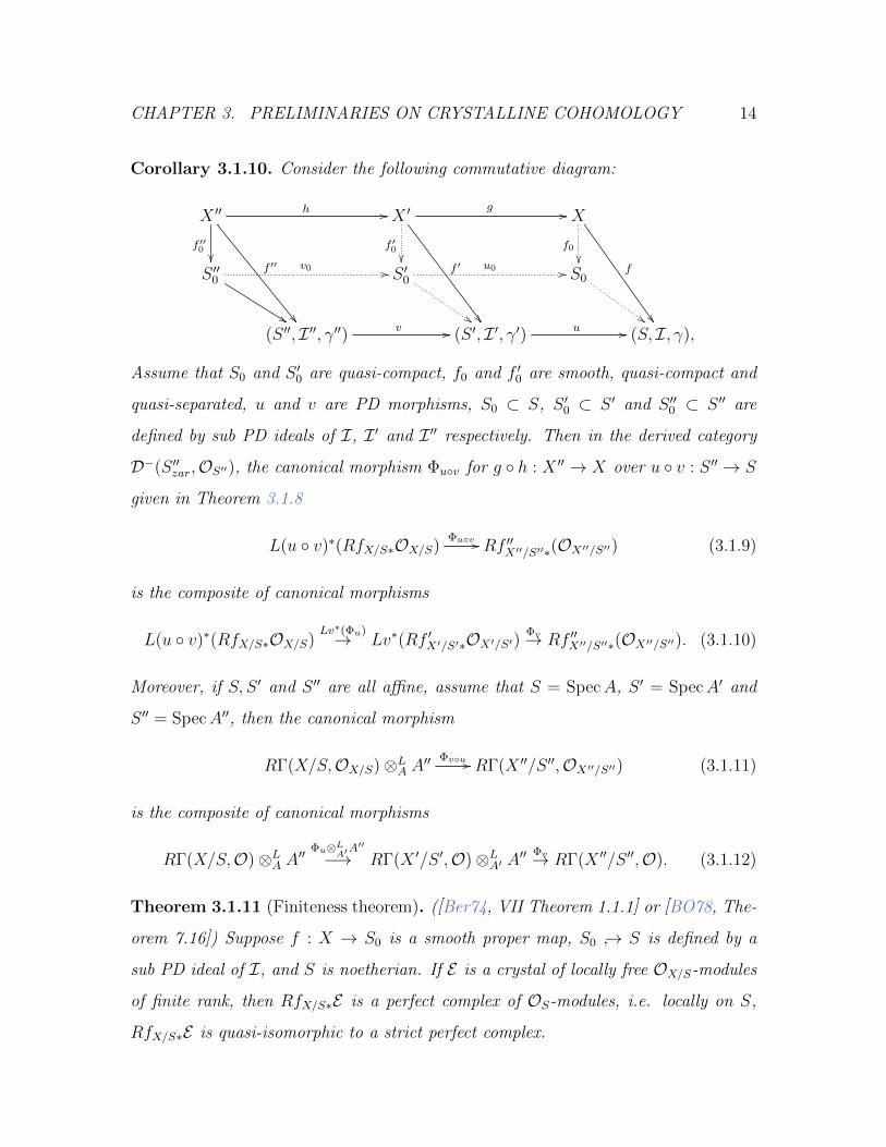
Corollary 3.1.10. Consider the following commutative diagram:
X ′′ h //
f ′′0
f ′′
X ′
f ′0
f ′
g // X
f0
f
S ′′0v0 //
%%
S ′0
$$
u0 // S0
##(S ′′, I ′′, γ′′) v // (S ′, I ′, γ′) u // (S, I, γ),
Assume that S0 and S ′0 are quasi-compact, f0 and f ′0 are smooth, quasi-compact and
quasi-separated, u and v are PD morphisms, S0 ⊂ S, S ′0 ⊂ S ′ and S ′′0 ⊂ S ′′ are
defined by sub PD ideals of I, I ′ and I ′′ respectively. Then in the derived category
D−(S ′′zar,OS′′), the canonical morphism Φuv for g h : X ′′ → X over u v : S ′′ → S
given in Theorem 3.1.8
L(u v)∗(RfX/S∗OX/S)Φuv // Rf ′′X′′/S′′∗(OX′′/S′′) (3.1.9)
is the composite of canonical morphisms
L(u v)∗(RfX/S∗OX/S)Lv∗(Φu)→ Lv∗(Rf ′X′/S′∗OX′/S′)
Φv→ Rf ′′X′′/S′′∗(OX′′/S′′). (3.1.10)
Moreover, if S, S ′ and S ′′ are all affine, assume that S = SpecA, S ′ = SpecA′ and
S ′′ = SpecA′′, then the canonical morphism
RΓ(X/S,OX/S)⊗LA A′′Φvu // RΓ(X ′′/S ′′,OX′′/S′′) (3.1.11)
is the composite of canonical morphisms
RΓ(X/S,O)⊗LA A′′Φu⊗LA′A
′′
−→ RΓ(X ′/S ′,O)⊗LA′ A′′Φv→ RΓ(X ′′/S ′′,O). (3.1.12)
Theorem 3.1.11 (Finiteness theorem). ([Ber74, VII Theorem 1.1.1] or [BO78, The-
orem 7.16]) Suppose f : X → S0 is a smooth proper map, S0 → S is defined by a
sub PD ideal of I, and S is noetherian. If E is a crystal of locally free OX/S-modules
of finite rank, then RfX/S∗E is a perfect complex of OS-modules, i.e. locally on S,
RfX/S∗E is quasi-isomorphic to a strict perfect complex.

CHAPTER 3. PRELIMINARIES ON CRYSTALLINE COHOMOLOGY 15
Corollary 3.1.12. [Ber74, VII Corollary 1.1.2] Under the hypotheses of Theorem
3.1.11, then for all i, RifX/S∗E is a coherent OS-module. Moreover if S is affine,
assume that A = Γ(S,OS), then for all i, H i(X/S, E) is a finitely generated A-module.
3.2 Crystalline cohomology over a p-adic base
3.2.1 Crystalline cohomology revisited
Situation 3.2.1.1. Let (A, I, γ) be a noetherian PD-ring together with a sub PD ideal
I0 of I such that I0 contains some prime number p, and A is I0-adically separated
and complete. For each n, we let An = A/In+10 , Sn = SpecAn and S = Spf A for the
I0-adic topology. And f : X → S0 is a proper smooth morphism.
The crystalline site Cris(X/S) of X relative to S include all objects of Cris(X/Sn)
for all n and can be viewed as a direct limit of the sites Cris(X/Sn) with the obvious
inclusions. Denote by (X/S)cris the topos of sheaves on Cris(X/S). For all n, there
exists a canonical morphism of topoi in : (X/Sn)cris → (X/S)cris.
Given a crystal E of locally free OX/S-modules of finite rank, then i∗nE is a crystal
over Cris(X/Sn). By (3.1.8), for every n, there exists a canonical isomorphism
RΓ(X/Sn+1, i∗n+1E)⊗LAn+1
An // RΓ(X/Sn, i∗nE) (3.2.1)
When varying n, we obtain a projective system in the sense of derived category.
Definition 3.2.1. Under the assumptions in Situation 3.2.1.1, the ith crystalline
cohomology of X relative to (A, I0, γ) is defined to be lim←−Hi(X/Sn,OX/Sn), denoted
by H icris(X/S). For a crystal E of locally free OX/S-modules of finite rank, we set
H i(X/S, E) = lim←−Hi(X/Sn, i
∗nE).
Remark 3.2.2. In [BO78], another appoach to define H i(X/S,O) via taking the de-
rived functors of Γ is applied to deal with the nonproper case. It is proved in [BO78,
Theorem 7.24.3] that the two approaches are equivalent under the assumption in
Situation 3.2.1.1

CHAPTER 3. PRELIMINARIES ON CRYSTALLINE COHOMOLOGY 16
Theorem 3.2.3 (Finiteness theorem). [Ber74, VII Proposition 1.1.5, Corollary 1.1.6]
Under the assumptions in Situation 3.2.1.1. Let E be a crystal of locally free OX/S-
modules of finite rank. Then there exists a strictly perfect complex, i.e. a bounded
complex of projective finite A-modules denoted by RΓ(X/S, E), such that:
1. For all n, there exists an isomorphism
RΓ(X/S, E)⊗A An∼ // RΓ(X/Sn, i
∗nE) (3.2.2)
in the derived category Db(Am), which is compatible with (3.2.1)
2. For all i, the natural homomorphism
H i(RΓ(X/S, E)) // lim←−Hi(X/Sn, i
∗nE) (3.2.3)
is an isomorphism. In particular, H i(X/S, E) is a finite A-module.
Proposition 3.2.4 (Flat base change). [Ber74, Proposition 1.1.8] Under the as-
sumptions in Situation 3.2.1.1. Let (A, I, γ)→ (A′, I ′, γ′) be a PD morphism. A′ is a
noetherian flat A-algebra PD-ring with a sub PD ideal I ′0 of I ′ such that I ′0 contains
I0A′, and A′ is I ′0-adically separated and complete. For each n, set A′n = A′/(I ′0)n+1,
S ′n = SpecA′n, S ′ = Spf A′ for the I0-adic topology and X ′ = X ×S0 S′0. Let E be a
crystal of locally free OX/S-modules of finite rank and E ′ be its the inverse image on
Cris(X ′/S ′). Then there exists an canonical isomorphism
H i(X/S, E)⊗A A′ // H i(X ′/S ′, E ′). (3.2.4)
An analogue of Theorem 3.1.8 over a p-adic base could be true, yet it does not
seem to exist in literature. We are going to show a result for base change to fibers.
Proposition 3.2.5. Under the assumptions in Situation 3.2.1.1. Take a point e :
Spec k → S0, where k is a perfect field. Let Xe = X ×e Spec k. Assume that e is a
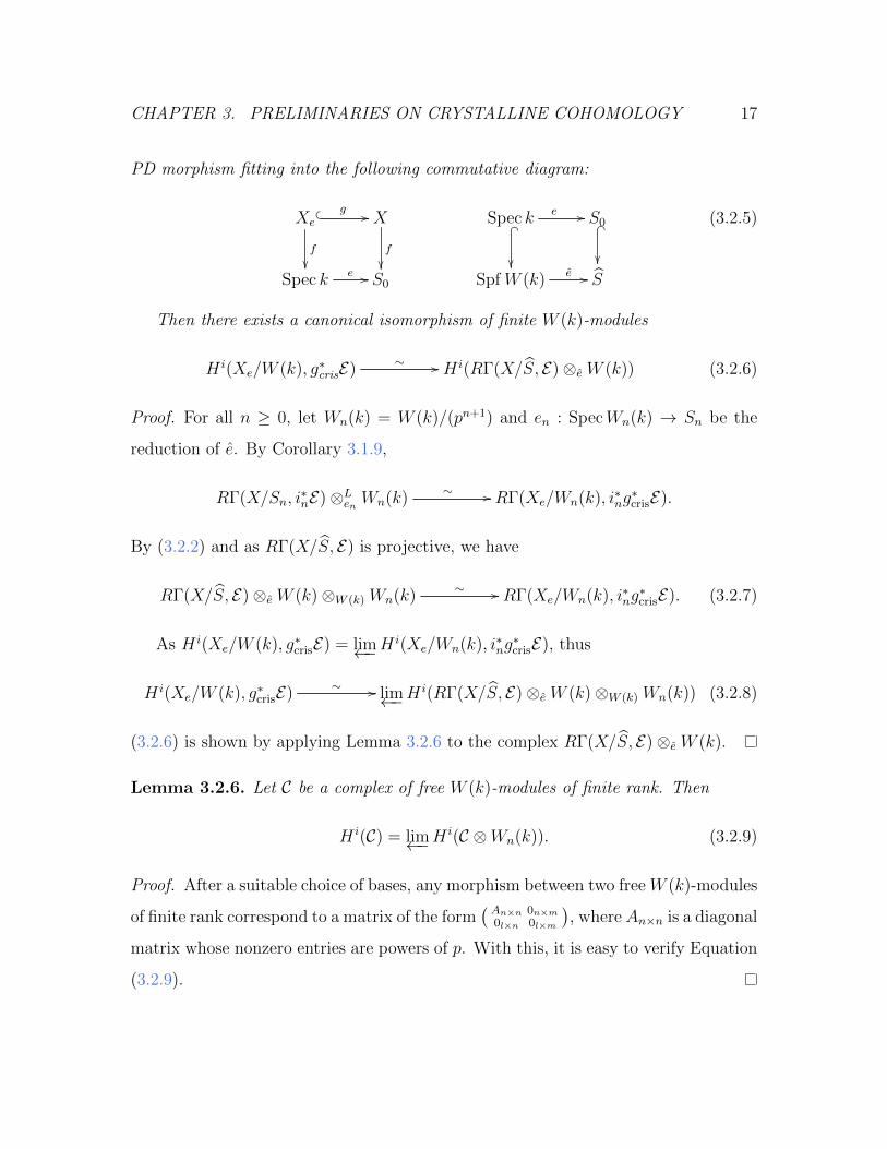
CHAPTER 3. PRELIMINARIES ON CRYSTALLINE COHOMOLOGY 17
PD morphism fitting into the following commutative diagram:
Xe
f
g // X
f
Spec k _
e // S0 _
Spec k e // S0 Spf W (k) e // S
(3.2.5)
Then there exists a canonical isomorphism of finite W (k)-modules
H i(Xe/W (k), g∗crisE) ∼ // H i(RΓ(X/S, E)⊗eW (k)) (3.2.6)
Proof. For all n ≥ 0, let Wn(k) = W (k)/(pn+1) and en : SpecWn(k) → Sn be the
reduction of e. By Corollary 3.1.9,
RΓ(X/Sn, i∗nE)⊗Len Wn(k) ∼ // RΓ(Xe/Wn(k), i∗ng
∗crisE).
By (3.2.2) and as RΓ(X/S, E) is projective, we have
RΓ(X/S, E)⊗eW (k)⊗W (k) Wn(k) ∼ // RΓ(Xe/Wn(k), i∗ng∗crisE). (3.2.7)
As H i(Xe/W (k), g∗crisE) = lim←−Hi(Xe/Wn(k), i∗ng
∗crisE), thus
H i(Xe/W (k), g∗crisE) ∼ // lim←−Hi(RΓ(X/S, E)⊗eW (k)⊗W (k) Wn(k)) (3.2.8)
(3.2.6) is shown by applying Lemma 3.2.6 to the complex RΓ(X/S, E)⊗eW (k).
Lemma 3.2.6. Let C be a complex of free W (k)-modules of finite rank. Then
H i(C) = lim←−Hi(C ⊗Wn(k)). (3.2.9)
Proof. After a suitable choice of bases, any morphism between two free W (k)-modules
of finite rank correspond to a matrix of the form( An×n 0n×m
0l×n 0l×m
), where An×n is a diagonal
matrix whose nonzero entries are powers of p. With this, it is easy to verify Equation
(3.2.9).

CHAPTER 3. PRELIMINARIES ON CRYSTALLINE COHOMOLOGY 18
3.2.2 Crystals revisited
First we recall a p-adic analogue of Proposition 3.1.4 to describe crystals in terms
of modules with connections. Such an analogue exists in a very general setting, see
[dJ95, Proposition 2.2.2] or [dJso, Proposition 40.22.4]. For our purpose of discussion,
we state the following analogy of Proposition 3.1.4.
Proposition 3.2.7. ([BM90, Proposition 1.3.3]) Given A0, A, An, S0 same as in Sit-
uations 4.1.0.1 or 4.1.0.2. Then the category of crystals of quasi-coherent OS0/Zp-
modules on Cris(S0/Zp) is equivalent to the category of separated, complete A-modules
with an integrable and topologically quasi-nilpotent connection.
When S0 = Spec k for a perfect k field, then a crystal of coherent OS0/Zp-modules
is a finite W (k)-module, as the condition on connection automatically holds.
Recall that a connection on an A-module is an additive morphism ∇ : M →
M ⊗ΩS/W (k) such that ∇(fm) = df ⊗m+ f∇(m), where ΩS/W (k) = lim←−ΩSn/Wn . We
say that∇ is topologically quasi-nilpotent with respect to a local coordinate xi if for
any section e, there are only finitely many pairs (i, k) such that ∇ki (e) /∈ pE , where ∇i
is the ∂∂xi
-derivative. For an integrable connection, being topologically quasi-nilpotent
is independent of the choice of local coordinates.
Now we turn to Frobenius structures on crystals. Given a morphism f : X → S0
in characteristic p, we denote by FX its absolute Frobenius endomorphism. Consider
the following commutative diagrams, where X ′ = X ×FS0S0.
XFX/S0 //
f
X ′WX/S0 //
f ′
X
f
S0
FS0 // _
S0 _
S0
FS0 // S0 , TFT // T ,
where T is a PD thickening of S0 and FT is a lifting of FS0 . T is p-adically complete
and of positive characteristic or characteristic 0.
By abuse of notations, we respectively denote by FX/T : (X,S0, T ) → (X ′, S0, T )

CHAPTER 3. PRELIMINARIES ON CRYSTALLINE COHOMOLOGY 19
and FT : (X ′, S0, T )→ (X,S0, T ) the following two diagrams:
X
FX/S0
f // S0 // T X ′
WX/S0
f ′ // S0
FS0
// T
FT
X ′f ′ // S0
// T , Xf // S0
// T .
Denote by FX,T : (X,S0, T )→ (X,S0, T ) the composite FT FX/T . Clearly F ∗X,T pulls
back crystals of OX/T -modules to crystals of OX/T -modules.
Recall that an F -crystal E over Cris(X/Zp) is defined to be a crystal of locally free
OX/Zp-modules of finite rank with a morphism Ψ : F ∗X,ZpE → E such that Ψ⊗Zp Qp is
an isomorphism. We generalize the concept of F -crystal as below:
Definition 3.2.8. Under the assumptions in Situations 4.1.0.1 or 4.1.0.2. An (F,∇)-
module over A is defined to be a triple (M,F,∇) consisting of a finite A-module M ,
a σ-linear morphism F : M →M and an integrable and topologically quasi-nilpotent
connection ∇ on M such that the linearization Ψ of F becomes an isomorphism after
tensoring with Qp and Ψ is a horizontal map when assuming M⊗σ A is endowed with
the induced connection from (M,∇). Denoted by (M,F,∇).
Remark 3.2.9. By Proposition 3.2.7, an (F,∇)-module is the same as a crystal E of
quasi-coherent, finitely generated OX/Zp-modules with a morphism Ψ : F ∗X,ZpE → E
such that Ψ ⊗Zp Qp is an isomorphism. In particular, an F -crystal is an (F,∇)-
module. In Situation 4.1.0.2, an (F,∇)-module is usually called as an (F, θ)-module,
see Definition 5.4.1.
For later use, we now give a description of the horizontal map Ψ : M ⊗σ A→ M
in Definition 3.2.8.
Lemma 3.2.10. Under the assumptions in Situations 4.1.0.1 or 4.1.0.2. The mor-
phism Ψ : M ⊗σ A → M in Definition 3.2.8 is horizontal if and only if the diagram

CHAPTER 3. PRELIMINARIES ON CRYSTALLINE COHOMOLOGY 20
as below is commutative:
M∇ //
F
M ⊗A ΩA/W (k)
F⊗FΩ
M ∇ //M ⊗A ΩA/W (k) ,
(3.2.10)
where ΩA/W (k) = lim←−ΩAn/Wn, FΩ = lim←−FΩ,n and FΩ,n : ΩAn/Wn → ΩAn/Wn is a
σ-linear map induced from σ : An → An.
Proof. The induced connection on M ⊗σ A is determined by a commutative diagram
as below:
M∇ //
q1
M ⊗A ΩA/W (k)
q1⊗FΩ
M ⊗σ A ∇f //M ⊗σ A⊗A ΩA/W (k) ,
(3.2.11)
where q1 is defined by m 7→ m⊗ 1. Ψ is a horizontal map if and only if it fits into a
commutative diagram as follows:
M ⊗σ A ∇f //
Ψ
M ⊗σ A⊗A ΩS/W (k)
Ψ⊗1Ω
M ∇ //M ⊗A ΩS/W (k) .
(3.2.12)
By combining (3.2.10) and (3.2.12), we prove the lemma.
CHAPTER 4. HICRIS(X/S) IS AN (F,∇)-MODULE 21
Chapter 4
Hicris(X/S) is an (F,∇)-module
In this chapter, we are going to show that in some cases, H icris(X/S) is an (F,∇)-
module. In other words, H icris(X/S) is similar to an F -crystal, except that it is not
locally free.
4.1 Preliminaries
We first list some facts and then propose two situations to be investigated.
Facts 4.1.1. ([Kat79, 2.4]) Let A0 be a smooth finitely generated algebra over a perfect
field k of characteristic p > 0. Then there exists a p-adically complete, flat W (k)-
algebra A and a homomorphism σ : A → A such that A/pA ' A0, An = A/(pn+1)
is formally smooth over Wn = W (k)/(pn+1) and σ is a (not unique) Frobenius lifting
of the absolute Frobenius morphism σ : A0 → A0. Moreover, there exists a unique
embedding iσ : A→ W (Apf0 ) compatible with Frobenius liftings.
Situation 4.1.0.1. Given A0, A and σ : A→ A same as in Fact 4.1.1. Let S0 = SpecA0,
Sn = SpecAn and S = Spf A. Let FSn ;Sn → Sn, FS : S → S be morphisms implied
by σ.
Situation 4.1.0.2. Given a perfect field k of characteristic p > 0. Let A0 = k[[t]],

CHAPTER 4. HICRIS(X/S) IS AN (F,∇)-MODULE 22
A = W (k)[[t]], An = A/(pn+1) = Wn[[t]] and fix σ : W (k)[[t]] → W (k)[[t]], t 7→ tp. Let
Sn, S, FSn , FS be similarly defined as in Situation 4.1.0.1.
Our purpose in this chapter is to prove the following statement:
Proposition 4.1.2. Given S0, S as in Situations 4.1.0.1 or 4.1.0.2. Let f : X → S0
be a proper smooth morphism. Then for all i, H icris(X/S) is an (F,∇)-module.
Proof. The above statement is a summary of Propositions 4.2.1, 4.3.1 and 4.4.1.
4.2 A σ-linear map F on H icris(X/S)
We may refer to Section 3.2.2 for some notations. The purpose of this section is to
prove
Proposition 4.2.1. With the assumptions in Proposition 4.1.2. Then there ex-
ists a σ-linear map F : H icris(X/S) → H i
cris(X/S) such that its linearization Ψ :
H icris(X/S)⊗σ A→ H i
cris(X/S) fitting into the following commutative diagram:
H icris(X/S)⊗σ A Ψ //
'
((
H icris(X/S)
H icris(X
′/S) .
RiFX/S
77(4.2.1)
Moreover, Ψ⊗Zp Qp is an isomorphism.
Proof. AsH icris(X/S) = lim←−H
i(X/Sn,OX/Sn), to obtain a σ-linear map onH icris(X/S),
it suffices to find a compatible system of σ-linear maps on H i(X/Sn,O),∀n. Consider
the following diagram of morphisms:
(X,S0, Sn)FX/Sn //
in,n+1
(X ′, S0, Sn)FSn //
in,n+1
(X,S0, Sn)
in,n+1
(X,S0, Sn+1)
FX/Sn+1// (X ′, S0, Sn+1)FSn+1// (X,S0, Sn+1) ,

CHAPTER 4. HICRIS(X/S) IS AN (F,∇)-MODULE 23
where in,n+1 : (X,S0, Sn)→ (X,S0, Sn+1) consists of the identity map of f : X → S0
and the closed immersion Sn → Sn+1. By applying Corollaries 3.1.9 and 3.1.10 to
OX/Sn+1 , we have a commutative diagram in Db(An) as follows:
RΓ(X/Sn) RΓ(X ′/Sn)oo RΓ(X/Sn)⊗Lσ An'oo
RΓ(X/Sn+1)⊗L An
OO
RΓ(X ′/Sn+1)⊗L Anoo
OO
RΓ(X/Sn+1)⊗Lσ An+1 ⊗L An'oo
OO
where RΓ(X/Sn) is RΓ(X/Sn,OX/Sn) for short. Note that σ : An → An is flat for
all n. After taking cohomology, we have a commutative diagram of An+1-modules as
follows:
H i(X/Sn,O) H i(X ′/Sn,O)oo H i(X/Sn,O)⊗σ An'oo
Ψntt
H i(X/Sn+1,O)
OO
H i(X ′/Sn+1,O)oo
OO
H i(X/Sn+1,O)⊗σ An+1 .'oo
OO
Ψn+1
jj
(4.2.2)
By taking inverse limit of (4.2.2), we get
Ψ : H i(X/S,OX/S)⊗σ A ' // H i(X ′/S,OX′/S)RiF
X/S// H i(X/S,OX/S). (4.2.3)
Moreover, by [BO83, Theorem 1.3], there exists an isomorphism
F ∗X/S
: Rif ′X′/S∗OX′/S ⊗Zp Qp
// RifX/S∗(OX/S)⊗Zp Qp (4.2.4)
induced by FX/S, where the functor fX/S is defined as follows:
fX/S : (X/S)crisuX/S// Xzar
fzar // (S)zar. (4.2.5)
Clearly Γ(S, RifX/S∗(OX/S)) = H icris(X/S), thus RiFX/S ⊗Zp Qp is an isomorphism,
so is Ψ⊗Zp Qp.
By applying Proposition 4.2.1 to a fiber Xe of f : X → S0 at the point e :
Spec k′ → S0, we obtain a σ-linear map on H icris(Xe/W (k)) as follows:
Ψe : H icris(Xe/W (k))⊗σ W (k′)→ H i
cris(Xe/W (k)). (4.2.6)
Now we are going to verify that the compatibility of Ψ with Ψe.

CHAPTER 4. HICRIS(X/S) IS AN (F,∇)-MODULE 24
Corollary 4.2.2. With the same assumptions as Proposition 4.1.2. Let e : Spec k′ →
S0 be a point of S0 and k′ is a perfect field. Let Xe = X×eSpec k. Let e : Spf W (k′)→
S be a canonical lifting of e such that e∗ : A → W (k′) is the composite map of iσ in
Fact 4.1.1 with the natural homomorphism W (Apf0 )→ W (k′). Then Ψ on H i
cris(X/S)
is compatible with Ψe on H icris(Xe/W (k)) in the following sense:
H icris(X/S)⊗σ A⊗eW (k′)
Ψ⊗id //
H icris(X/S)⊗eW (k′)
H i
cris(Xe/W (k′))⊗σ W (k′)Ψe // H i
cris(Xe/W (k′)) ,
(4.2.7)
where the vertical maps are induced from (3.2.6).
Proof. Let Wn = W (k)/(pn+1) and denote by en : (Xe, k′,Wn) → (X,S0, Sn) the
diagram:
Xe
f // Spec k′
e
// SpecWn
en
Xf // S0
// Sn .
(4.2.8)
Consider the following diagram of morphisms:
(Xe, k′,Wn)
FXe/Wn//
en
(X ′e, k′,Wn)
FWn //
en
(Xe, k′,Wn)
en
(X,S0, Sn)FX/Sn // (X ′, S0, Sn)
FSn // (X,S0, Sn) ,
By applying Corollaries 3.1.9 and 3.1.10 to OX/Sn , we have a commutative diagram
in D−(Wn) as follows:
RΓ(Xe/Wn) RΓ(X ′e/Wn)oo RΓ(Xe/Wn)⊗Lσ Wn'oo
RΓ(X/Sn)⊗Len Wn
OO
RΓ(X ′/Sn)⊗Len Wnoo
OO
RΓ(X/Sn)⊗Lσ An ⊗Len Wn'oo
OO

CHAPTER 4. HICRIS(X/S) IS AN (F,∇)-MODULE 25
After taking cohomology, we have
H i(Xe/Wn,O) H i(X ′e/Wn,O)oo H i(Xe/Wn,O)⊗σ Wn'oo
H i(X/Sn,O)⊗en Wn
OO
H i(X ′/Sn,O)⊗en Wnoo
OO
H i(X/Sn,O)⊗σ An ⊗en Wn .'oo
OO
(4.2.9)
It is easy to see that (4.2.9) forms a diagram of inverse systems when varying n. By
taking inverse limit, we obtain (4.2.7).
By Proposition 3.2.4, H icris(Xe/W (k)) behaves properly under field extension, as
a consequence of Corollary 4.2.2, we see that the σ-linear maps are compatible under
base change.
Corollary 4.2.3. Let X be a proper smooth scheme over a perfect field k of charac-
teristic p > 0. Assume that k′ ⊃ k is a perfect field extension and Xk′ = X ×k k′.
Then we have a commutative diagram as below:
H icris(X/W (k))⊗σ W (k)⊗W (k) W (k′) //
'
H icris(X/W (k))⊗W (k) W (k′)
'
H icris(Xk′/W (k′))⊗σ W (k′) // H i
cris(Xk′/W (k′)) ,
(4.2.10)
where the the vertical isomorphisms are given by (3.2.4) and the horizontal maps are
isomorphic after tensoring with Qp.
4.3 A connection ∇ on H icris(X/S)
In this section, we are going to introduce an integrable and topologically quasi-
nilpotent connection ∇ on H icris(X/S).
Proposition 4.3.1. With the same assumptions as Proposition 4.1.2. Then there
exists an integrable, topologically quasi-nilpotent W (k)-connection
∇ : H icris(X/S)→ H i
cris(X/S)⊗A ΩA/W (k). (4.3.1)

CHAPTER 4. HICRIS(X/S) IS AN (F,∇)-MODULE 26
Proof. As H icris(X/S) = lim←−H
i(X/Sn,OX/Sn), we first introduce an integrable, quasi-
nilpotent connection on H i(X/Sn,OX/Sn) for every n. By Proposition 3.1.4, the
data of an integrable, quasi-nilpotent connection is equivalent to the data of an
HPD stratification. Thus it remains to check the existence of HPD stratifications
on H i(X/Sn,OX/Sn). This will be done by definition, similar to the proof of [Ber74,
V Corollary 3.6.3].
Denote by Dn(ν) the divided power envelope of Sn as a closed subscheme of
(Sn/Wn)(ν+1) under the diagonal immersion4 : Sn → Dn(ν+1). Let pk : Dn(1)→ Sn
for k = 1, 2 be the two natural projections. Let DAn/Wn(ν) = Γ(Dn(ν),ODn(ν)).
First, to define a compatible system of DAn/Wn(1)-linear isomorphisms
εn : DAn/Wn(1)⊗An H i(X/Sn,OX/Sn)→ H i(X/Sn,OX/Sn)⊗An DAn/Wn(1), (4.3.2)
we consider a commutative diagram as follows
(X,S0, Sn) _
(X,S0, Dn(1)) _
p1oo p2 // (X,S0, Sn) _
(X,S0, Sn+1) (X,S0, Dn+1(1))
p1oo p2 // (X,S0, Sn+1) .
(4.3.3)
By applying Corollaries 3.1.9 and 3.1.10 to , we obtain a commutative diagram as
follows:
RΓ(X/Sn+1)⊗Lp1DAn+1/Wn+1(1)
' // RΓ(X/Dn+1(1))
DAn+1/Wn+1(1)⊗Lp2RΓ(X/Sn+1)
'oo
RΓ(X/Sn)⊗Lp1DAn/Wn(1) ' // RΓ(X/Dn(1)) DAn/Wn(1)⊗Lp2
RΓ(X/Sn)'oo
As p1, p2 are flat by Remark 3.1.7, after taking cohomology, we obtain the following
commutative diagram with OX/Sn removed from H i(X/Sn,OX/Sn) for short:
H i(X/Sn+1)⊗p1 DAn+1/Wn+1(1)
' // H i(X/Dn+1)
DAn+1/Wn+1(1)⊗p2 Hi(X/Sn+1)
'oo
εn+1ss
H i(X/Sn)⊗p1 DAn/Wn(1) ' // H i(X/Dn) DAn/Wn(1)⊗p2 Hi(X/Sn).'oo
εn
kk
(4.3.4)

CHAPTER 4. HICRIS(X/S) IS AN (F,∇)-MODULE 27
Thus we obtain a compatible system of isomorphisms εn. It is routine to verify
that εn is a compatible system of HPD stratifications, and we omit the lengthy de-
tails. Note that the connection ∇n : H i(X/Sn,OX/Sn)→ H i(X/Sn,OX/Sn)⊗ΩAn/Wn
induced from εn is integrable and quasi-nilpotent by Proposition 3.1.4, therefore,
∇ = lim←−∇n is integrable and topologically quasi-nilpotent.
Remark 4.3.2. Recall from Proposition 3.1.4, ∇n induced from εn is defined as below:
H i(X/Sn)εnq2−q1 // H i(X/Sn)⊗An DAn/Wn(1)
mod J[2]n // H i(X/Sn)⊗ Ω1
An/Wn, (4.3.5)
where q2 and q1 are the natural projection morphisms, Jn is the PD ideal of 4∗ :
DAn/Wn(1) → An and J[2]n is the PD ideal generated by J2
n, see definition in [BO78,
Definition 3.24]
4.4 The compatibility of F with ∇
Proposition 4.4.1. With the same assumptions as Proposition 4.1.2. The σ-linear
map F : H icris(X/S) → H i
cris(X/S) given in Proposition 4.2.1 is a horizontal map
with respect to the connection ∇ given in 4.3.1, i.e. (F,∇) fits into (3.2.10).
Proof. As H icris(X/S) = lim←−H
i(X/Sn,OX/Sn), it suffice to show that for every n, the
diagram as below is commutative:
H i(X/Sn,OX/Sn)∇n //
Fn
H i(X/Sn,OX/Sn)⊗An ΩAn/Wn
Fn⊗FΩ,n
H i(X/Sn,OX/Sn)
∇n // H i(X/Sn,OX/Sn)⊗An ΩAn/Wn ,
(4.4.1)
where Fn is the σ-linear map induced from Ψn given in Proposition 4.2.1. As ∇n
is deduced from an HPD stratification εn by (4.3.5), it suffices to show that εn is
compatible with Fn. Consider a commutative diagram as below:
(X,S0, Sn)
FX,Sn
(X,S0, Dn(1))
FX,Dn
p1oo p2 // (X,S0, Sn)
FX,Sn
(X,S0, Sn) (X,S0, Dn(1))p1oo p2 // (X,S0, Sn) .
(4.4.2)

CHAPTER 4. HICRIS(X/S) IS AN (F,∇)-MODULE 28
Then apply Corollaries 3.1.9 and 3.1.10 to OX/Sn , we have a commutative diagram:
RΓ(X/Sn)⊗Lp1DAn/Wn(1)
Fn⊗FDn
' // RΓ(X/Dn(1))
DAn/Wn(1)⊗Lp2RΓ(X/Sn)
FDn⊗Fn
'oo
RΓ(X/Sn)⊗Lp1DAn/Wn(1) ' // RΓ(X/Dn(1)) DAn/Wn(1)⊗Lp2
RΓ(X/Sn) ,'oo
(4.4.3)
where FDn : DAn/Wn(1) → DAn/Wn(1) is a σ-linear map induced from σ : An → An,
the vertical map in the middle is FDn-linear. As p1, p2 are flat, by taking cohomology,
we obtain
H i(X/Sn)⊗p1 DAn/Wn(1)
Fn⊗FDn
' // H i(X/Dn(1))
DAn/Wn(1)⊗p2 Hi(X/Sn)
FDn⊗Fn
'oo
εntt
H i(X/Sn)⊗p1 DAn/Wn(1) ' // H i(X/Dn) DAn/Wn(1)⊗p2 Hi(X/Sn) .'oo
εn
kk
(4.4.4)
This completes the proof of the proposition.
Now we turn to a morphism h : X ′ → X of proper smooth S0-schemes: Then
there is a canonical morphism given by (3.1.7):
H icris(X/S)
Φh // H icris(X
′/S). (4.4.5)
With a similar proof as Proposition 4.4.1, we see that Φh is a morphism (F, θ)-
modules, i.e. Φh commutes with the σ-linear maps and is a horizontal map with
respect to the connections.
Proposition 4.4.2. Given S0, S as in Situations 4.1.0.1 or 4.1.0.2. Given a mor-
phism h : X ′ → X of proper smooth S0-schemes. Then for all i, the canonical
morphism Φh is a morphism of (F, θ)-modules.

CHAPTER 5. NEWTON POLYGONS AND SPECIALIZATION THEOREM 29
Chapter 5
Newton polygons and
specialization theorem
Given a smooth proper morphism X → S0, we will introduce two types of Newton
polygons associated to every point e of S0, one from the crystalline cohomology group
H icris(Xe/W (k′),OXe/W (k′)) and the other from the base change of H i
cris(X/S) to e. We
will see that on a nonempty open subscheme U ⊂ S0 the above two types of Newton
polygons coincide; moreover, in Situation 4.1.0.2, we will show that the above two
types of Newton polygons coincide everywhere and there exists an F -crystal with the
same Newton polygons and isogenous to the (F,∇)-module H icris(X/S). This result
makes it possible to apply the known results for F -crystals to prove both specialization
and purity theorems of crystalline cohomology.
5.1 Basics about Newton polygons
In this section, we first recall the definition of Newton polygons associated to F -
crystals over a perfect field k, and then introduce two types of Newton polygons.
Recall that the notion of an F -crystal over a perfect field k of characteristic p > 0
is equivalent to a pair (M,F ) consisting of a finite free W (k)-module M together

CHAPTER 5. NEWTON POLYGONS AND SPECIALIZATION THEOREM 30
with a σ-linear endomorphism F : M →M such that F ⊗Zp Qp is an automorphism,
where σ : W (k)→ W (k) is the absolute Frobenius. Newton slopes of (M,F ), roughly
speaking, are the p-adic values of “eigenvalues” of F . Precisely, they can be defined
as follows: choose an integer N ≥ 1 divisible by r!, r = rank M , and consider the
discrete valuation ring
R = W (k)[X](XN − p) = W (k)[p1/N ], (5.1.1)
where k is an algebraic closure of k. Extend σ to R by requiring that σ(X) = X and
extend F to a σ-linear map of M ⊗W (k) K, where K is the fraction field of R. By
Dieudonne’s theory ([Man63]), M ⊗W (k) K admits a K-basis e1, · · · , er such that
F (ei) = pλiei, λi ∈ Q≥0. (5.1.2)
The rational numbers λ1, · · · , λr are called Newton slopes of (M,F ).
We may assume that λ1 ≤ · · · ≤ λr. The Newton polygon of (M,F ), denoted by
NP(M,F ) is the graph of the Newton function on [0, r] defined on integers by
NewtonF (i) = λ1 + · · ·+ λi for 1 ≤ i ≤ r and 0 for i = 0. (5.1.3)
Let mult(λ) be the number of times that λ occurs among (λ1, . . . , λr). Then by
Dieudonne’s theory,
Σλ∈Qmult(λ) = r, λ ·mult(λ) ∈ Z
In other words, break points of Newton polygons where Newton slopes jump are
integral.
Similarly we can define Newton polygon of an (F,∇)-module over W (k), which
is usually called as an F -module over W (k), since the connection is insignificant. It
is easy to see that Newton polygon is invariant under isogeny, i.e. NP(M1, F1) =
NP(M1, F1) if there exists an isogeny φ : (M1, F1) → (M2, F2) of F -modules, which
is defined to be a morphism φ : M1 → M2 such that F2 φ = φ F1 and φ ⊗ Qp is
isomorphic
Now we are ready to define two types of Newton polygons.

CHAPTER 5. NEWTON POLYGONS AND SPECIALIZATION THEOREM 31
Definition 5.1.1. Let f : X → S0 be a proper smooth morphism of schemes in
characteristic p > 0. For every point e ∈ S0, choose a perfect field k′ such that e
is the image of e : Spec k′ → S0. Recall the notations Xe, e and Ψe from Corollary
4.2.2. We define a Newton polygon associated to (e, i, f) to be the Newton polygon
of the F -module (H icris(Xe/W (k′)),Ψe), denote by NP1(e, i). Note that NP1(e, i) is
independent of the choice of k′ by Corollary 4.2.3.
To define the second type of Newton polygon, we require the assumptions of
Proposition 4.1.2. With the notations e,Xe, e same as above. We turn to the (F,∇)-
module H icris(X/S). Let Mi,e = H i
cris(X/S) ⊗e∗ W (k′). Note that Mi,e naturally
becomes an F -module with a σ-linear map induced from that on H icris(X/S), i.e.
H icris(X/S) F //
H icris(X/S)
H icris(X/S)⊗e∗ W (k′)('Mi,e)
Fi,e // H icris(X/S)⊗e∗ W (k′)('Mi,e) .
(5.1.4)
Definition 5.1.2. Under the assumptions of Proposition 4.1.2, the second type of
Newton polygon associated to e is the Newton polygon of (Mi,e, Fi,e), denoted by
NP2(e, i). Note that NP2(e, i) is independent of the choice of k′.
By (4.2.7), we have a commutative diagram as below:
Mi,e ⊗σ W (k′)Ψi,e //
χe⊗id
Mi,e
χe
H icris(Xe/W (k′))⊗σ W (k′)
Ψe // H icris(Xe/W (k′)) ,
(5.1.5)
we will show that for points of an open subscheme, χe ⊗ Qp is isomorphic, i.e. Mi,e
and H icris(Xe/W (k′)) are isogenous and thus NP1(e, i) = NP2(e, i).
5.2 Comparison of Newton polygons
To compare NP1(e, i) with NP2(e, i), we will need a lemma as follows:
CHAPTER 5. NEWTON POLYGONS AND SPECIALIZATION THEOREM 32
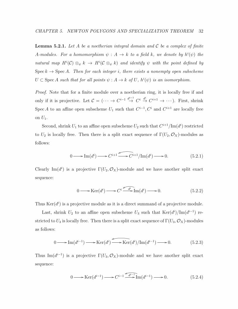
Lemma 5.2.1. Let A be a noetherian integral domain and C be a complex of finite
A-modules. For a homomorphism ψ : A → k to a field k, we denote by hi(ψ) the
natural map H i(C) ⊗ψ k → H i(C ⊗ψ k) and identify ψ with the point defined by
Spec k → SpecA. Then for each integer i, there exists a nonempty open subscheme
U ⊂ SpecA such that for all points ψ : A→ k of U , hi(ψ) is an isomorphism.
Proof. Note that for a finite module over a noetherian ring, it is locally free if and
only if it is projective. Let C = (· · · → Ci−1 di−1
→ Ci di→ Ci+1 → · · · ). First, shrink
SpecA to an affine open subscheme U1 such that Ci−1, Ci and Ci+1 are locally free
on U1.
Second, shrink U1 to an affine open subscheme U2 such that Ci+1/Im(di) restricted
to U2 is locally free. Then there is a split exact sequence of Γ(U2,OX)-modules as
follows:
0 // Im(di) // Ci+1 // Ci+1/Im(di) //uu
0. (5.2.1)
Clearly Im(di) is a projective Γ(U2,OX)-module and we have another split exact
sequence:
0 // Ker(di) // Ci di // Im(di) //yy
0. (5.2.2)
Thus Ker(di) is a projective module as it is a direct summand of a projective module.
Last, shrink U2 to an affine open subscheme U3 such that Ker(di)/Im(di−1) re-
stricted to U3 is locally free. Then there is a split exact sequence of Γ(U3,OX)-modules
as follows:
0 // Im(di−1) // Ker(di) // Ker(di)/Im(di−1) //ss
0. (5.2.3)
Thus Im(di−1) is a projective Γ(U3,OX)-module and we have another split exact
sequence:
0 // Ker(di−1) // Ci−1 di−1// Im(di−1) //
uu0. (5.2.4)

CHAPTER 5. NEWTON POLYGONS AND SPECIALIZATION THEOREM 33
With (5.2.1), (5.2.2), (5.2.3) and (5.2.4), we have a commutative diagram as follows:
Ci−1 di−1//
'
Ci di //
'
Ci+1
'
Ker(di−1)⊕ Im(di−1)
( 0 id0 00 0
)// Im(di−1)⊕ Ker(di)
Im(di−1)⊕ Im(di)
(0 0 id0 0 0
)// Im(di)⊕ Ci+1
Im(di).
Clearly for every point ψ : A→ k of U3, the natural map hi(ψ) is an isomorphism.
Now we show that NP1(e, i) = NP2(e, i) for points of an open subscheme.
Corollary 5.2.2. With the assumptions of Proposition 4.1.2. There exists a nonempty
open subscheme U ⊂ S0 such that for all points e : Spec k′ → U , the morphism
χe : Mi,e → H icris(Xe/W (k′)) in (5.1.5) is an isogeny of F -modules and NP1(e, i) =
NP2(e, i).
Proof. We may assume that S0 is irreducible. By Theorem 3.2.3, there exists of a
strictly perfect complex RΓ(X/S,OX/S) such that H icris(X/S) = H i(RΓ(X/S,OX/S))
and H icris(Xe/W (k′)) ∼ // H i(RΓ(X/S,OX/S)⊗eW (k′)) by (3.2.6).
By applying Lemma 5.2.1 to the complex RΓ(X/S,OX/S), we may assume that
there exists an open affine subscheme Spec A[ 1α
] ⊂ Spec A such that for every point
ψ of Spec A[ 1α
], hi(ψ) is isomorphic. Assume that α = pnβ with β ∈ A\pA. Let
α0 = (β mod p) ∈ A0 and U = SpecA0[ 1α0
]. Consider the canonical lifting e :
Spf W (k′)→ S for every point e : Spec k′ → U , note that the homomorphism
e∗ ⊗Qp : A→ W (k′) → W (k′)⊗Zp Qp
factors through A[ 1α
] and can be viewed as a point of Spec A[ 1α
]. Therefore, for every
point e : Spec k′ → U , hi(e∗⊗Qp) is an isomorphism. Moreover, it is easy to see that
hi(e∗ ⊗Qp) is exactly χe ⊗Qp in (5.1.5). This completes the proof.
5.3 Specialization theorem for F -prelattices
As the proof of specialization theorem for F -crystals [Kat79, Theorem 2.3.1] only
involves the Frobenius structure, it can be employed to prove similar property for

CHAPTER 5. NEWTON POLYGONS AND SPECIALIZATION THEOREM 34
objects endowed with only the Frobenius structure, for example, F -prelattices.
Definition 5.3.1. In Situation 4.1.0.1, an F -prelattice over A is a pair (M,F ) con-
sisting of a finite A-module M and a σ-linear map F : M → M such that the
linearization Ψ : M ⊗σ A → M becomes an isomorphism after tensoring with Qp.
Denoted by (M,Ψ).
Clearly the (F,∇)-module H icris(X/S) is an F -prelattice over A. Given an F -
prelattice, same as defining NP2(e, i) in Definition 5.1.2, we can associate a Newton
polygon to every point e of S0, denoted by NP(e,M).
Lemma 5.3.2 (Specialization theorem for F -prelattice). In Situation 4.1.0.1, let
(M,F ) be an F -prelattice over A. Then there exists an open subscheme U ⊂ S0 such
that the family of Newton polygons NP(e,M) | e ∈ U is constant.
Proof. Without loss of generality, we may assume that S0 is irreducible. First there
exists an open affine subscheme Spec A[ 1α
] such thatM⊗AA[ 1α
] is a free A[ 1α
]-module of
finite rank. Assume that α = pnβ with β ∈ A\pA. Let α0 = (β mod p) ∈ A0 and U =
SpecA0[ 1α0
]. It is easy to see that the composite map Aiσ //W (Apf
0 ) //W (Apf0 [ 1
α0])[1
p]
factors through A[ 1α
]. Let R = W (Apf0 [ 1
α0]). Clearly M ⊗A R[1
p] is a free R[1
p]-module
of finite rank and the σ-linear map F : M ⊗A R[1p] → M ⊗A R[1
p] can be expressed
as a matrix with entries in R[1p]. We may replace F by pn0F so that all entries of the
matrix of F are in R. Let λ1 ≤ . . . ≤ λr be the Newton slopes of NP(η,M) at the
generic point of S0. By a similar proof to that of ([Kat79, Theorem 2.3.1]), we see
that for every 1 ≤ i ≤ r, the set of points in SpecA0[ 1α0
] at which all Newton slopes
of (∧iM,∧iF ) are =∑i
k=1 λk is a Zariski open subset. This proves the lemma.
Remark 5.3.3. A key step in the proof of [Kat79, Theorem 2.3.1] is to apply basic
slope estimate [Kat79, 1.4.3] to convert the condition on Newton slopes to conditions
on Hodge slopes, which can be described in terms of entries of the matrix of the
σ-linear map.

CHAPTER 5. NEWTON POLYGONS AND SPECIALIZATION THEOREM 35
Corollary 5.3.4. With the assumptions of Proposition 4.1.2. There exists a nonempty
open subscheme U ⊂ S0 such that the family of Newton polygons NP1(e, i) | e ∈ U
is constant.
Proof. May assume that S0 is irreducible. First, by Corollary 5.2.2, there exists a
nonempty open subscheme U1 ⊂ S0 such that for all points e ∈ U1, NP1(e, i) =
NP2(e, i). Then apply Lemma 5.3.2 to H icris(X/S), we obtain an open subscheme
U2 ⊂ S0 such that the family of Newton polygons NP2(e, i) | e ∈ U2 is constant.
Thus U = U1 ∩ U2 is as required.
5.4 F -Crystals isogenous to H icris(X/S)
In this section, we restrict to Situation 4.1.0.2 when S0 = Spec k[[t]] and show that
there exists an F -crystal over Cris(S0/W (k)) isogenous to the (F,∇)-moduleH icris(X/S).
In this case, an (F,∇)-module is usually called as an (F, θ)-module defined as below.
Definition 5.4.1. [dJ98, Definition 4.9] In Situation 4.1.0.2, an (F, θ)-module over
A = W (k)[[t]] is a triple (M,F, θ) consisting of a finitely generated A-module, a σ-
linear map F : M →M and an additive map θ : M →M such that
1. The A-linear morphism M ⊗σ A→M becomes isomorphic after tensoring with
Qp;
2. θ(fm) = fθ(m) + ddt
(f)m, where ddt
: A→ A is defined by Σantn 7→ Σnant
n−1;
3. θ(F (m)) = ptp−1F (θ(m)).
An isogeny of (F, θ)-modules is a morphism φ : (M,F, θ) → (M ′, F ′, θ′) such that
φ⊗A KW [[t]] become an isomorphism, where KW = W (k)[1p].
Note that θ is the same as an connection, which is automatically integrable.

CHAPTER 5. NEWTON POLYGONS AND SPECIALIZATION THEOREM 36
Definition 5.4.2. We say that an (F, θ)-module (M,F, θ) has a topologically quasi-
nilpotent connection if for every m ∈ M , there exists some k > 0 such that θk(m) ∈
pM .
Given an (F, θ)-module, similarly as Definition 5.1.2, we can associate a Newton
polygon to both points of S0. Clearly, Newton polygons are invariant under isogeny.
We will first see some properties of (F, θ)-modules.
Lemma 5.4.3. Let (M,F, θ) be an (F, θ)-module over A = W (k)[[t]] and KW be the
fraction field of W (k). Then M ⊗A KW [[t]] is a free KW [[t]]-module.
Proof. Let MK = M⊗AKW [[t]] and M τK ⊂MK be the maximal submodule of torsions.
To see M τK = 0, we first prove by induction on n that if m ∈ M τ
K satisfies that
tnm = 0, then m ∈ tM τK . Note that θ extends to MK . The initial case: n = 1, i.e.
tm = 0, then θ(tm) = tθ(m) +m = 0 and m ∈ tM τK . The induction step: if tnm = 0,
then θ(tnm) = tnθ(m) + ntn−1m = 0. Since tn−1(tθ(m) + nm) = 0, by assumption,
tθ(m)+nm ∈ tM τK , thus m ∈ tM τ
K . By induction, M τK ⊂ tM τ
K . Then by Nakayama’s
Lemma, M τK = 0.
Lemma 5.4.4. ([dJ98, Lemma 6.1]) Let (M,F, θ) be an (F, θ)-module over A =
W (k)[[t]]. Then there exists an isogeny M → M ′ to a free (F, θ)-module over A. If
(M,F ′, θ′) has a topologically quasi-nilpotent connection, so does (M ′, F, θ).
Proof. See [dJ98, Lemma 6.1]. As A is regular local of dimension 2, the dual of a
finitely generated A-module is finite free. We may take M ′ as below:
M ′ = HomA(HomA(M, A), A). (5.4.1)
The evaluation map ev : M → M ′ has a finite length cokernel. The fact that ev ⊗AKW [[t]] is an isomorphism follows from Lemma 5.4.3.
Let KA is the fraction field of A. M ′ can also be viewed as a submodule of
M ⊗A KA consisting of m ∈ M ⊗A KA such that m1 = pn1m,m2 = tn2m ∈ M for

CHAPTER 5. NEWTON POLYGONS AND SPECIALIZATION THEOREM 37
some n1, n2 ∈ N and tn2m1 = pn1m2 in M . From this point of view, it is easy to check
that the (F, θ)-actions on M extends to (F ′, θ′)-actions on M ′. Moreover, if θ on M
is topologically quasi-nilpotent, then for every m ∈M and every N > 0, there exists
some k > 0 such that θk(m) ∈ pN+1M . Thus for every m′ ∈ M ′ of the form mpN
, we
have (θ′)k(m′) ∈ pM ′. Therefore, θ′ on M ′ is topologically quasi-nilpotent.
Before replacing H icris(X/S) by an isogenous F -crystal, we would like to verify
that NP1(e, i) = NP2(e, i) for both points e ∈ Spec k[[t]].
Lemma 5.4.5. Given S0, S as in Situations 4.1.0.2. Let s and η respectively be the
special and generic point of S0 = Spec k[[t]]. Let f : X → S0 be a proper smooth
morphism. Then NP1(e, i) = NP2(e, i) for both points of S0; NP1(s, i) and NP1(η, i)
have the same endpoints.
Proof. NP1(η, i) = NP2(η, i) follows from Corollary 5.2.2. If e = s, we need to review
the map χe in (5.1.5). Note that A = W (k)[[t]] and s∗ : A → W (k) is defined by
t 7→ 0. By (3.2.6), χs is given as follows (write RΓ(X/S,OX/S) as RΓ(X/S) for short
):
H i(RΓ(X/S))⊗s∗ W (k)χs // H i(RΓ(X/S)⊗s∗ W (k)). (5.4.2)
To show that NP1(s, i) = NP2(s, i), it suffices to show χs ⊗W (k) KW is an isomor-
phism. LetKW be the fraction field ofW (k). Still denote by s∗ the mapKW [[t]]→ KW
given by t 7→ 0. Let C be the complex RΓ(X/S,OX/S) ⊗A KW [[t]]. As the natural
map A = W (k)[[t]]→ KW [[t]] is flat, we have a commutative diagram as below:
H i(RΓ(X/S))⊗s∗ W (k)⊗KWχs⊗KW //
'
H i(RΓ(X/S)⊗s∗ W (k))⊗KW
'
H i(C)⊗s∗ KWχ′e // H i(C ⊗s∗ KW ) ,
(5.4.3)
Then apply the universal coefficient theorem to the complex C of finite free KW [[t]]-
modules and s∗ : KW [[t]]→ KW , we obtain an exact sequence
0→ H i(C)⊗s∗ KW → H i(C ⊗s∗ KW )→ Tor1(KW [[t]]/(t), H i+1(C))→ 0, (5.4.4)

CHAPTER 5. NEWTON POLYGONS AND SPECIALIZATION THEOREM 38
where Tor1(KW [[t]]/(t), H i+1(C)) = m ∈ H i+1(C) | tm = 0. Since H i+1(C) '
H i+1cris (X/S) ⊗A KW [[t]] and H i+1
cris (X/S) is an (F, θ)-module over A, by Lemma 5.4.3,
H i+1cris (X/S) ⊗A KW [[t]] is free, so is H i+1(C). Therefore, χ′s is an isomorphism, so is
χs ⊗W (k) KW . Thus NP1(s, i) = NP2(s, i).
To see that NP1(s, i) and NP1(η, i) have the same endpoints, it suffices to show
that NP2(s, i) and NP2(η, i) have the same endpoints. Since NP 2(e, i) is based on the
(F, θ)-module H i(C) and H i(C) ⊗A KW [[t]] is a free KW [[t]]-module by Lemma 5.4.3,
it is not hard to see that NP2(s, i) and NP2(η, i) have the same endpoints (r, nr),
where r = rank H i(C)⊗AKW [[t]] and nr is the p-adic value of the determinant of the
σ-linear self-map of H i(C).
Now we are ready to claim that H icris(X/S) is isogenous to an F -crystal.
Proposition 5.4.6. With the assumptions in Lemma 5.4.5. Then there exists an
isogeny ξ : H icris(X/S) → Pi of (F, θ)-modules to a free (F, θ)-module (Pi, F, θ) over
A with a topologically quasi-nilpotent connection; NP1(e, i) = NP(e, Pi) for both points
of S0. Denote by Pi the F -crystal over Cris(Spec k[[t]]/Zp) corresponding to (Pi, F, θ).
Proof. It follows from Lemmas 5.4.4 and 5.4.5.
Corollary 5.4.7. With the notations in Lemma 5.4.5. NP1(s, i) lies on or over
NP1(η, i).
Proof. It follows from applying Grothendieck’s specialization theorem [Kat79, Theo-
rem 2.3.1] to the F -crystal Pi in Proposition 5.4.6.
Remark 5.4.8. The above proof also implies that NP1(s, i) and NP1(η, i) have the
same endpoints.
CHAPTER 5. NEWTON POLYGONS AND SPECIALIZATION THEOREM 39
5.5 Specialization theorem of crystalline cohomol-
ogy
In this section, we reprove the specialization theorem of crystalline cohomology. First
we generalize Corollary 5.3.4 to the case when S0 is not necessarily smooth.
Lemma 5.5.1. Consider a proper smooth morphism f : X → S0 over an affine and
irreducible Fp-scheme S0 of finite type. Let η ∈ S0 be the generic point. Then there
exists an open subscheme U ⊂ S0 such that NP1(e, i) = NP1(η, i) for all e ∈ U .
Proof. Let S0 be the normalization of S0 in its function field. By [Mat80, 31.H],
h : S0 → S0 is a finite and surjective morphism. As S0 is normal, then it has a
smooth open affine subscheme U0. As U0 is affine, smooth and of finite type over Fpand f ′ : X ×S0 U0 → U0 is proper smooth, the assumptions of Corollary 5.3.4 are
satisfied, thus there exists an open subscheme U1 ⊂ U0 such that the family of Newton
polygons NP1(e, i)|e ∈ U1 is constant. As h is an open map, then h(U1) ⊂ S0 is an
open subscheme as required.
Theorem 5.5.2 (Speciallization). Let S be an Fp-scheme and f : X → S be a
proper smooth morphism. Then there exists a locally finite stratification S =∐
α Uα
consisting of locally closed subsets of S such that for every α, the family of Newton
polygons NP1(e, i)|e ∈ Uα is constant. Moreover, if η is a generization of s, then
NP1(s, i) lies on or over NP1(η, i) and they have the same endpoints.
Proof. First, because of the local nature of the theorem, we may assume that S =
SpecA is affine. Second, by EGA IV 8.9.1, 8.10.5 and 17.7.8, there exists an affine
Fp-scheme S0 of finite type, a proper smooth morphism f0 : X0 → S0 and a cartesian
diagram:
X //
f
X0
f0
S
π // S0 .
(5.5.1)

CHAPTER 5. NEWTON POLYGONS AND SPECIALIZATION THEOREM 40
As π−1closed set = closed set and π−1open set = open set, it suffices to
prove the theorem for f0. May assume that S is an affine and irreducible Fp-scheme
of finite type.
By Lemma 5.5.1 and EGA 0III9.2.6, we conclude that the stratification by Newton
polygons consists of a finite disjoint union of locally closed subsets.
To see that Newton polygons rise under specialization from η to s, we first find a
morphism Spec k[[t]]→ S such that it maps the special and generic point of Spec k[[t]]
to s and η respectively, where k is a perfect field. Then the proof is done by applying
Lemma 5.4.5 and Corollary 5.4.7 to the base change of f under Spec k[[t]]→ S.

CHAPTER 6. REPRESENTATIONS AND PURITY THEOREM 41
Chapter 6
Representations and purity
theorem
We are going to prove a purity theorem of crystalline cohomology. The proof is similar
as that of [Yan11, Theorem 1.1]. A key point in the proof is to employ an equivalence
between the unramified property of representations and the coincidence of Newton
polygons.
6.1 Rank-1 representations associated to F -modules
In this section, k will denote a perfect field of characteristic p > 0, unless otherwise
specified. Set Galk = Aut(ksep/k). Note that for a perfect field k, the separable
closure ksep is also the algebraic closure k. The following fact will be very useful to
make transitions between a field and its perfect closure.
Facts 6.1.1. ([Rom06, Theorems 3.6.1, 3.6.4]) Let k be a field of characteristic p > 0
and k be its algebraic closure. Let ksep and kpf be the separable and perfect closure
of k inside k respectively. Denote by Galk (resp. Galkpf ) the automorphism group of

CHAPTER 6. REPRESENTATIONS AND PURITY THEOREM 42
ksep (resp. k ) over k (resp. kpf). Then there exists a canonical isomorphism
Galk ' Aut(k/k) ' Galkpf . (6.1.1)
We first define a representation for a rank-one F -crystal.
Definition 6.1.2. Let (M,F ) be a rank-one F -crystal over a perfect field k and e
be a basis. Assume that F (e) = pmµe for some unit µ ∈ W (k). Extend (M,F ) to an
F -crystal over k. By Dieudonne’s theory ([Man63]), there exists a unit α ∈ W (k) such
that F (αe) = pmαe, i.e. µ · σ(α) = α. With the Galois action Galk on k canonically
lifted to an action on W (k), we can define a representation as follows:
ρM : Galk → Z∗p, g 7→ g(α) · α−1. (6.1.2)
We would like to define representations depending on break points of Newton
polygons. To do this, we first manage to find an F -crystal of rank 1 as follows:
Proposition 6.1.3. ([Yan11, Proposition 2.1]) Let (M,F ) be an F -crystal over a
perfect field k of characteristic p > 0. If the first break point of NP(M) is (1, N) for
N ∈ N, then (M,F ) has a unique subcrystal M1 ⊂ M of rank 1 and slope N such
that any subcrystal of slope N is a subcrystal of M1.
Proof. See [Yan11, Proposition 2.1].
Start with a break point (r,N) of the Newton polygon of an F -crystal (M,F ), we
consider the exterior power (∧rM,∧rF ), which is an F -crystal with (1, N) as its first
break point. By applying Proposition 6.1.3 to (∧rM,∧rF ), we find an F -crystal M1
of rank 1 and then obtain a representation from M1 by applying Definition 6.1.2.
Definition 6.1.4. Let (M,F ) be an F -module over W (k) and β be a break point of
NP(M). Take the maximal free submodule M ′ ⊂M . Note that M ′ naturally becomes
an F -crystal and NP(M ′) = NP(M). We define the representation associated to
(M,β) to be the one induced from (M ′, β) shown as above, denoted by ρ(M,β) :
Galk → Z∗p.

CHAPTER 6. REPRESENTATIONS AND PURITY THEOREM 43
Facts 6.1.5. Given an isogeny (M,F ) → (M ′, F ′) of F -modules over W (k) and a
break point β of NP(M) = NP(M ′). Then the representations ρ(M,ξ) and ρ(M ′,ξ) are
the same.
Now we define a representation induced from an (F, θ)-module.
Definition 6.1.6. Let (M,F, θ) be an (F, θ)-module over A = W (k)[[t]]. Fix a
morphism η : Spec k((t))pf → Spec k[[t]] to the generic point η ∈ Spec k[[t]] and
take the canonical lifting η∗ : W (k)[[t]] → W (k((t))pf). With a break point β of
NP1(η,M) of the F -module M ⊗η∗ W (k((t))pf), by Definition 6.1.4, we obtain a map
ρ : Galk((t))pf → Z∗p. We define the representation associated to (η,M, β) to be the
composite map Galk((t)) ' Galk((t))pfρ→ Z∗p, denoted by ρ(η,M,β). Note that ρ(η,M,β) is
invariant under isogeny of (F, θ)-modules.
We are interested in representations induced from crystalline cohomology groups.
Definition 6.1.7. Let f : X → S0 be a proper smooth morphism of schemes in
characteristic p > 0. For every point e ∈ S0, let ke be the residue field at e and
Xkpfe
be the base change of f to kpfe , a perfect closure of ke. With a break point
β of NP1(e, i) of the F -module H icris(Xe/W (kpf
e )), by Definition 6.1.4, we obtain a
map ρ : Galkpfe→ Z∗p. With the canonical isomophism Galke ' Galkpf
ein Facts
6.1.1, we define the representation associated to (e,H icris, β) to be the composite map
Galke ' Galkpfe
ρ→ Z∗p, denoted by ρ(e,i,β).
We would like to see how representations are related under base change.
Lemma 6.1.8. With the assumptions in Definition 6.1.7. Let k′ ⊃ kpfe be a per-
fect field and e′ : Spec k′ → S0. Then ρ(e,i,β),k′ is isomorphic to the representation
associated to (e′, H icris(Xk′/W (k′)), β), where
ρ(e,i,β),k′ : Galk′ → Galkeρ(e,i,β)−→ Z∗p. (6.1.3)
Proof. It follows from an isomorphism of F -modules in Corollary 4.2.3.

CHAPTER 6. REPRESENTATIONS AND PURITY THEOREM 44
Corollary 6.1.9. With the assumptions in Proposition 5.4.6. Let η be the generic
point of S0 = Spec k[[t]] and β be a break point of NP1(η, i) = NP(η, Pi). Then ρ(η,i,β)
and ρ(η,Pi,β) are the same representation Galk((t)) → Z∗p.
Proof. By Proposition 5.4.6, H icris(X/S) and Pi are isogenous, thus ρ(η,Hi
cris(X/S),β) =
ρ(η,Pi,β) by Definition 6.1.6. Apply Corollary 5.2.2 to the generic point η : Spec(k((t)))pf →
S0, we obtain an isogeny of F -modules; by Facts 6.1.5, ρ(η,Hicris(X/S),β) = ρ(η,i,β) .
6.2 Criteria for unramified representations
For F -crystals over Cris(Spec k[[t]]/Zp), we have an equivalence between unramified
representations and coincidence of break points; we show an analogous equivalence
for the cohomology case. First we recall the equivalence for F -crystals.
Proposition 6.2.1. ([Yan11, Proposition 4.4]) Let R be a discrete valuation ring
of characteristic p > 0 with fraction field K and residue field k. Let E be an F -
crystal over Spec R. Let η and s be the generic and closed point of Spec R. Assume
that the first break point of NP (E)η is (1,m). Then the following two conditions are
equivalent:
1. the Galois representation associated to E is unramified, i.e., it factors through
φ : GalK → π1(Spec R).
2. the first break point of NP (E)s is (1,m).
Proof. See [Yan11, Proposition 4.4] or below for a sketch of the proof for the case
when R = k[[t]] with k algebraically closed. The general case can be reduced to
this case following similar discussion as the proof of Proposition 6.2.2. In this case,
π1(SpecR) is trivial, thus it turns to show that (1) the associated representation to
E is trivial if and only if (2) (1,m) is also the first break point of NP (E)s.

CHAPTER 6. REPRESENTATIONS AND PURITY THEOREM 45
(1)⇒(2): By [Yan11, Lemma 4.3], ESpec K has a trivial subcrystal of rank 1 and
slope m. Then we get an injection Φ : LSpecK → ESpec K , where L is a trivial F -crystal
of rank 1 and slope m over Spec R. Apply [dJ98, Theorem 1.1] to E ,L and Φ. We
obtain a nontrivial map L → E . Restricting to s,we see that Es contains a subcrystal
of rank 1 and slope m. On the other hand, by Grothendieck’s specialization theorem
[Kat79, 2.3.1], NP (E)s lies on or above NP (E)η. Hence (1,m) is the first break point
of NP (E)s.
Condition (2)⇒ (1):by [Kat79, Corollary 2.6.2], E is isogenous to an F -crystal E ′
which is divisible by pm, which contains a subcrystal E ′1 of rank 1 and slope m. By
[Kat79, Theorem 2.7.4], E ′1 becomes isogenous to a constant F -crystal over k((t))pf ,
and therefore the associated representation to E ′1 is trivial. As representations asso-
ciated to F -crystals are preserved under isogeny, thus we obtain (1).
Now we show a similar equivalence for the cohomology case.
Proposition 6.2.2. Let R be a discrete valuation ring of characteristic p > 0 with
fraction field K and residue field k and f : X → SpecR be a proper smooth mor-
phism. Let η and s respectively be the generic and special point of SpecR. Let β be a
break point of NP1(η, i). Then β is a break point of NP1(s, i) if and only if the repre-
sentation ρ(η,i,β) : GalK // Z∗p is unramified, i.e., it factors through the canonical
map GalKφ // π1(SpecR) .
For the proof, we recall a lemma regarding the kernel of GalKφ // π1(SpecR) .
Lemma 6.2.3. ([Yan11, Corollary 3.4]) Let R be a discrete valuation ring of char-
acteristic p > 0 with fraction field K and residue field k. Let R be the completion of
R and fix an isomorphism R = k[[t]]. Let k be the algebraic closure of k. Then the
kernel of the canonical homomorphism GalKφ // π1(SpecR) is the normal subgroup
of GalK generated by the image of the composition Galk((t))// Galk((t))
// GalK .
Proof. See [Yan11, Corollary 3.4].

CHAPTER 6. REPRESENTATIONS AND PURITY THEOREM 46
Proof of Proposition 6.2.2. We first prove the case when R = k[[t]] for a perfect field
k. May assume that β is the first break point, as other cases are reduced to this
one by taking exterior powers. By Proposition 5.4.6 and Corollary 6.1.9, there exists
an F -crystal Pi over S0 = Spec k[[t]] such that NP1(e, i) = NP(e, Pi) for both points
of S0 and ρ(η,Pi,β) = ρ(η,i,β). Thus the proposition in this case follows directly from
Proposition 6.2.1.
In the general case, let R be the completion of R and fix an isomorphism R = k[[t]].
Consider the base change of f to Spec kpf[[t]] and let K1 = kpf((t)). On the one hand,
by Corollary 4.2.3, NP1(η, i) is invariant under base change. On the other hand,
by Lemma 6.1.8, the representation associated to (η,H icris(XKpf
1/W (Kpf
1 )), β) is the
composite map ρ(η,i,β),K1 : GalK1// GalK
ρ(η,i,β)// Z∗p . Clearly
ρ(η,i,β),K1 is unramified.
⇐⇒ Galk((t)) ⊂ GalK1 is in the kernel of ρ(η,i,β),K1 .
⇐⇒ The composite map Galk((t))// Galk((t))
// GalKρ(η,i,β)// Z∗p is trivial.
⇐⇒ ρ(η,i,β) is unramified. (By Lemma 6.2.3)
Thus the general case follows from the case for R = kpf[[t]].
6.3 Purity theorem of crystalline cohomology
The proof of purity theorem (Theorem 6.3.4) applies the same method as [dJO99,
Theorem 4.1] and [Yan11, Theorem 1.1]. We first prove purity theorem in a special
case (Theorem 6.3.3), then complete the proof of Theorem 6.3.4 by reducing the
general case to the case in Theorem 6.3.3. Now we list some facts to be referred to
in the proof.
Facts 6.3.1. ([Neu99, II Propostion 5.5]) Let Tp = 1 + p2Zp be a subgroup of
(Z∗p, ∗). There exists an isomorphism (Tp, ∗)log→ (p2Zp,+), 1 + x 7→ log(1 + x) =

CHAPTER 6. REPRESENTATIONS AND PURITY THEOREM 47
∑∞n=0
(−1)n
n+1xn+1. We fix an isomorphism (Tp, ∗) ' (Zp,+) to be log composite with
(p2Zp,+) ' (Zp,+).
Lemma 6.3.2. Let f : X → S0 be a proper smooth morphism of schemes in charac-
teristic p > 0. Consider the cartesian diagram as below:
Xf // S0 3 g(e′) Spec kg(e′)
X ′
OO
f ′ // S ′0 3 e′g
OO
Spec ke′
OO(6.3.1)
Let ke′ (resp. kg(e′)) be the residue field at e′ ∈ S ′0 (resp. g(e′) ∈ S ′0). Then we have
1. NP1(e′, i) = NP1(g(e′), i).
2. For any break point β of NP1(e′, i), the representation ρ(e′,i,β) is the composite
map of the canonical map Galke′ → Galkg(e′) with ρ(g(e′),i,β).
Proof. (1) follows from Corollary 4.2.3 and invariance of Newton polygons under
isogeny; (2) follows from Lemma 6.1.8. They will respectively be referred to as invari-
ance of Newton polygons and compatibility of representations under base change.
Theorem 6.3.3. Let (A,m, k) be a Noetherian complete local normal integral domain
of dimension 2 and its residue field k be algebraically closed. Assume that S0 = SpecA
and f : X → S0 is a proper smooth morphism. Let e0 ∈ S0 be the closed point and
U = S0\e0 be the open subscheme. If the family of Newton polygons NP1(e, i) | e ∈
U have a common break point β, then β is also a break point of NP1(e0, i).
Proof. Let η be the generic point of S0 and K be the fraction field of A. Consider
ρ(η,i,β) : GalK → Z∗p. First, we may assume that ρ(η,i,β)(GalK) ⊂ Tp, the latter
introduced in Facts 6.3.1. Otherwise we take a finite Galois extension L of K such
that ρ(η,i,β)(GalL) ⊂ Tp, replace A by the integral closure A′ of A inside L and f by
its base change to S ′0 = SpecA′. Let e′0 be the closed point of S ′0 and U ′ = S ′0\e′0.
Note that A′ have the same properties as A, the natural map S ′0 → S0 maps e′0 to e0
CHAPTER 6. REPRESENTATIONS AND PURITY THEOREM 48
and U ′ to U . By invariance of Newton polygons under base change, the general case
reduces to the case when ρ(η,i,β)(GalK) ⊂ Tp.
Second, we show that ρ(η,i,β) factors through the canonical map GalK → π1(U).
By [Yan11, Prop 3.2], it suffices to show that for every e ∈ U , ρ(η,i,β) factors through
GalK → π1(SpecOU,e), where OU,e is the local ring at e. Consider the base change
of f to SpecOU,e, denoted by fe. By Lemma 6.3.2, ρ(η,i,β) can be viewed as coming
from fe; and the Newton polygon associated to both points of SpecOU,e have the
same break points. By applying Proposition 6.2.2 to fe, we obtain that ρ(η,i,β) factors
through GalK → π1(SpecOU,e). Therefore, ρ(η,i,β) factors through GalK → π1(U).
Consider the composite map
GalK // π1(U) //
ι))
Tp' // Zp. (6.3.2)
Next, take a resolution of singularities S0 → S0; if A happens to be regular, let
S0 be the blowup of S0 with respect to e0. By [dJO99, Theorem 3.2], H1et(S0,Qp) '
H1et(U,Qp), thus ι defined in (6.3.2) viewed as an element of H1
et(U,Qp) is extended
to an element of H1et(S0,Qp), i.e. ι factors through π1(U) → π1(S0). Let η0 be the
generic point of some connected component of the exceptional fiber and OS0,η0be the
local ring at η0. We have the following commutative diagram:
GalK //
ρ(η,i,β)
++π1(U) //
ι
&&
TpOO
'
X ×S0 SpecOS0,η0
fη0
π1(SpecOS0,η0) // π1(S0) // Zp SpecOS0,η0
.
(6.3.3)
Note that ρ(η,i,β) viewed as the representation associated to the generic point of
SpecOS0,η0, is unramified as shown above. By applying Proposition 6.2.2 to fη0 ,
we see that β is a break point of NP1(η0, i) = NP1(e0, i).
Theorem 6.3.4 (Purity). Let S0 be a locally Noetherian scheme of characteristic
p > 0 and f : X → S0 be a proper smooth morphism. Take a point e0 ∈ S. If
the family of Newton polygons NP1(e, i) | e is a generization of e0 have a common

CHAPTER 6. REPRESENTATIONS AND PURITY THEOREM 49
break point β, then either the codimension of the Zariski closure of e0 in S0 is ≤ 1,
or β is a break point of NP1(e0, i).
Proof. Let e0− be the Zariski closure of e0 in S0. May assume that codim(e0−, S0) ≥
2, then it suffices to show that β is a break point of NP1(e0, i). First, consider the
base change fe0 of f to SpecOS0,e0 , where OS0,e0 is the local ring at e0. By invariance
of Newton polygons under base change, it reduces to prove the theorem for fe0 . We
may assume that S0 = SpecR of dimension ≥ 2, where R is a local Noetherian ring
and e0 is the closed point.
Note that if there exists a morphism of local rings ψ : R → R′ such that the
induced morphism of schemes g : S ′0 → S0 maps all points other than the close point
to the open subscheme S0\e0, and R′ is a Noetherian complete local normal integral
domain of dimension 2 with an algebraically closed residue field, then consider the
base change f ′ of f to S ′0, by invariance of Newton polygons under base change, it
reduces to prove the theorem for f ′, which is proved in Theorem 6.3.3.
Therefore, it suffices to find a morphism ψ : R→ R′ satisfying the above assump-
tions. First take the completion R of R. By Cohen structure theorem, we may assume
that R = k[[x1, . . . , xd]]/I for some ideal I, where k is the residue field. Second, con-
sider Rk = k[[x1, . . . , xd]]/Ik[[x1, . . . , xd]], where k is the algebraic closure of k. Next,
choose a prime ideal p ⊂ Rk such that A = Rk/p is of dimension 2. The existence
of such a prime ideal is shown in [Mat80, Proposition 12.K]. Last, take the integral
closure A of A in its fraction field. So far, we have obtained a chain of morphisms as
below:
R //ψ
--R // Rk// A // A
k[[x1, . . . , xd]]/I // k[[x1, . . . , xd]]/Ik[[x1, . . . , xd]] // Rk/p
(6.3.4)
We claim that ψ : R → A is as required. First, A is a finite A-module by [Mat80,
Corollary(Nagata)]; as a finite algebra over a henselian ring and also as an integral

CHAPTER 6. REPRESENTATIONS AND PURITY THEOREM 50
domain, A is a local ring by [Mil80, Theorem 4.2]. It is easy to check that ψ satisfies
all other assumptions. This completes the proof.

51
Part II
Representations and
Frobenius-periodic vector bundles

CHAPTER 7. INTRODUCTION 52
Chapter 7
Introduction
It was conjectured by de Jong in [dJ01, Conjecture 2.3] that given a finite field F of
characteristic l and a normal variety Y over a finite field κ of characteristic p 6= l,
every representation ρ : π1(Y ) → GL(r,F((s))) has a finite geometric monodromy.
This conjecture was proved by de Jong in the GL2-case [dJ01], by Bockle–Khare in
the GLn-case under some mild condition [BK06] and by Gaitsgory modulo the theory
of F((s))-sheaves [Gai07]. Then a natural question comes up: if the hypothesis l 6= p
is dropped and moreover Y is proper over κ, does the conjecture remain true? Note
that when Y/κ is not proper, a counterexample has already been given in [dJ01]
In [Las01], Laszlo gave a negative answer to the above question. He showed that
there exists a non-trivial family of rank-2 bundles fixed by the square of Frobenius
over a specific genus-2 curve C0/F2. From this he deduced the existence of the desired
representations of π1(C0⊗F2d). Recently, Esnault and Langer [EL11] have employed
Laszlo’s example to improve the statement of a p-curvature conjecture in characteristic
p.
It is suspected by de Jong that the representations with an infinite geometric
monodromy are rare. Thus one would like to understand the underlying mechanics
of Laszlo’s example and to obtain such representations in other characteristics.
In this part, we give a geometric interpretation of Laszlo’s example based on the

CHAPTER 7. INTRODUCTION 53
study of the action of the automorphism group of the curve; this interpretation allows
us to produce a family of similar examples. Meanwhile, our method also provides some
indication in characteristics 3 and 5, though it does not directly provide examples.
Now we give a brief summary of our results. In [Las01], Laszlo deduced represen-
tations from a non-trivial family of bundles. We show that the converse also holds, see
Theorem 8.3.1. The equivalence between a non-constant family of stable Frobenius-
periodic vector bundles and a representation with an infinite geometric monodromy
is of course well-known to the experts.
Because of the equivalence in Theorem 8.3.1, the question of looking for represen-
tations with an infinite geometric monodromy is converted to studying the fixed point
locus of the rational map V :MY (r, 0) //MY (r, 0) defined by taking pullback of
vector bundles under the geometric Frobenius of Y/κ. In [Las01], the expression of
VC0 for the specific curve C0 was applied to locate a projective line 4 in MC0(2, 0)
such that (V 2C0
)|4 is the identity map. Here our observation is that 4 is the fixed
point locus of the G-action onMC0(2, 0), where G = Aut(C0⊗F22/F22) = Z/2Z×S3.
Indeed, this property is common to all genus-2 ordinary curves X in characteristic 2
with a G-action. As Frobenius morphisms commute with the G-actions, it is natural
to consider the restriction of V to the fixed point locus MX(2, 0)G of the G-action
on MX(2, 0). With some trick, we manage to show that some power of V restricted
to MX(2, 0)G is the identity map and thus obtain a family of curves that carry a
non-constant family of stable Frobenius-periodic vector bundles, see Theorem 9.3.1.
Moreover, we give an explicit construction of the family of vector bundle, see Lemma
10.1.1 and Corollary 10.3.3.
Combining with Theorem 8.3.1, for every curve in Theorem 9.3.1, there exist
representations of the fundamental group with an infinite geometric monodromy.
A large part of the proof of Theorem 9.3.1 can be applied to other characteristics,
particularly the application of a group action in locating a sublocus in the moduli
space. However, when considering whether the restriction of the Verschiebung to

CHAPTER 7. INTRODUCTION 54
the sublocus is reduced to a linear map, the condition regarding the existence of
a single base point on the sublocus is sufficient only in charateristic 2. In other
characteristics, more is required to ensure that the restriction of the Verschiebung is
the identity. Examples of representations with an infinite geometric monodromy in
charateristic other than 2 remain to be discovered.

CHAPTER 8. FROBENIUS-PERIODIC BUNDLES 55
Chapter 8
Frobenius-periodic bundles and
Representations
8.1 Definitions and basic properties
In this section, we establish equivalences among the categories of Frobenius-periodic
vector bundles, smooth etale sheaves and representations.
Notations: κ is a finite field of order q = pd, S = Specκ[[s]], S = Spf κ[[s]] and
Sn = Specκ[[s]]/(sn) for n ≥ 0; FY is the absolute Frobenius of a noetherian κ-scheme
Y .
8.1.1 Smooth etale κ[[s]]-sheaves
Our definition of smooth etale κ[[s]]-sheaves is similar to that of a lisse l-adic sheaf
in [Mil80, Chap.V, §1]. When Y is connected, there is an equivalence between the
category of locally free smooth κ[[s]]-sheaves over Yet and the category of continuous
π1(Y )-modules that are free κ[[s]]-modules of finite rank, denoted by C1,Yet C2,π1(Y ).
Definition 8.1.1. Let Y be a noetherian scheme. An etale κ[[s]]-sheaf (or sheaf of
κ[[s]]-modules) on Yet is a projective system F = (Fn)n∈N of sheaves on Yet such that

CHAPTER 8. FROBENIUS-PERIODIC BUNDLES 56
the given map Fn+1 → Fn is isomorphic to the canonical map Fn+1 → Fn+1 ⊗κ[[s]]
κ[[s]]/(sn) for every n. Implicitly, F0 = 0 and Fn is a κ[[s]]/(sn)-module. A κ[[s]]-
sheaf is locally constant or constructible if each Fn has the corresponding property.
A locally constant constructible κ[[s]]-sheaf is also called smooth. A κ[[s]]-sheaf F is
locally free of rank r if each Fn is locally free of rank r over κ[[s]]/(sn).
Similarly, the stalk functor F // Fy = lim←−(Fn)y defines an equivalence
between the category of constructible, locally constant κ[[s]]-sheaves over Yet and the
category of continuous π1(Y, y)-modules that are finitely generated.
Facts 8.1.2. Assume that Y is a connected noetherian scheme with geometric point
y. Then there is an equivalence between the category CYet of locally free smooth κ[[s]]-
sheaves over Yet and the category Cπ1(Y ) of continuous π1(Y, y)-modules that are free
κ[[s]]-modules of finite rank, given by F // Fy = lim←−(Fn)y. Denoted by CYet
Cπ1(Y ).
8.1.2 Frobenius-periodic bundles
Now we turn to Frobenius-periodic bundles.
Definition 8.1.3. Let Y and T be noetherian κ-schemes. A vector bundle F over
Y ×κ T is said to be Frobenius-periodic if ∃ an isomorphism ξ : F → (F dY × idT )∗F
(resp. ξ : F → (F dY × idSn)∗F), denoted by (F , ξ). A Frobenius-periodic vector bundle
(F , ξ) over Y ×κ S is a projective system ((Fn, ξn))n∈Z+ such that for each n, (Fn, ξn)
is a Frobenius-periodic vector bundle over Y ×κ Sn, the given map Fn+1 → Fn is
isomorphic to the natural map Fn+1 → Fn+1 ⊗κ[[s]] κ[[s]]/(sn) and compatible with
ξn’s.
For any morphism Zf→ Y , the pull back of a Frobenius-periodic vector bundle
(F , ξ) over Y ×κ T to Z ×κ T can be viewed as a Frobenius-periodic vector bundle
over Z ×κ T , denoted by f ∗(F , ξn) or (f ∗F , f ∗ξ).

CHAPTER 8. FROBENIUS-PERIODIC BUNDLES 57
Definition 8.1.4. Given a Frobenius-periodic vector bundle (F , ξ) over Y ×κ T . A
section s ∈ Γ(Y ×κ T,F) is said to be fixed by ξ if ξ(s) = (F dY × idT )∗s; (F , ξ) is said
to be trivializable if F has a global basis fixed by ξ; it is said to be etale trivializable
if there exists a finite etale map Zf→ Y such that f ∗(F , ξ) is trivializable. In this
case we also say that Z/Y trivializes (F , ξ).
Given a Frobenius-periodic vector bundle (Fn, ξn) over Y ×κSn, we define an etale
sheaf (Fn)ξn as follows:
(Uf→ Y ) ∈ Et(Y )
// s ∈ Γ(U, f ∗F)|f ∗(ξ)(s) = 1⊗ s. (8.1.1)
We are going to see that (Fn)ξn is a locally free smooth κ[[s]]/(sn)-sheaf. In the
following, by a covering space of Y , we mean a finite etale morphism f : Z → Y and
it is Galois if #Aut(Z/Y ) = deg(f).
Lemma 8.1.5. Given a Frobenius-periodic vector bundle (F , ξ) = ((Fn, ξn))n∈Z+ over
Y×κS. Then there exists a family of covering spaces Y ← Y1 ← Y2 ← · · · ← Yn ← · · ·
such that for all n, Yn/Y trivializes (Fn, ξn).
Proof. According to [Mil80, V Proposition 1.1], a locally constant sheaf with finite
stalks over Yet is represented by a finite etale group scheme over Y . Thus, for every
n, to show that (Fn, ξn) is etale trivializable, it suffices to show that the etale sheaf
(Fn)ξn associated to (Fn, ξn) is locally constant and has finite stalks.
Prove by induction on n. Case n = 1 is exactly [LS77, Proposition 1.2]. First
there exists an open covering Uα of Y such that F1|Uα×κS1 is free for all α. We are
going to see that for every Uα, there exists a finite etale morphism U ′α → Uα that
trivializes (F1, ξ1)|Uα×κS1 . let v1, ..., vr be a basis of F1|Uα×κS1 . Assume that
ξ1v1, ..., vr = (F dY × idS1)∗v1, ..., (F
dY × idS1)∗vrN0,
for some N0 ∈ GL(r,OY (Uα)). To find a basis v′1, ..., v′r of the form v1, ..., vrM1
that is fixed by ξ1, it is equivalent to find M1 = (mij)ri,j=1 such that
N0M1 ≡M(q)1 , where M
(q)1 = (mq
ij), q = pd.

CHAPTER 8. FROBENIUS-PERIODIC BUNDLES 58
Thus we define Uα,1 = SpecOY (Uα)[m11, ...,mrr, 1/det M1]/(N0M1−M (q)1 ). It is easy
to see that U ′α → Uα is finite etale and trivializes (F1, ξ1)|Uα×κS1 . Therefore, the etale
sheaf (F1)ξ1 is locally constant and has finite stalk κ⊕r.
Induction step: assume that there is a covering space Yn → Y that factors
through Yn−1 and trivializes (Fn, ξn). Take an open covering Uα of Yn such that
Fn+1|Uα×κSn+1 is free for all α. We are going to see that for every Uα, there exists a
finite etale morphism U ′α → Uα that trivializes (Fn+1, ξn+1)|Uα×κSn+1 . Let v1, ..., vr
be a basis of Fn+1|Uα×κSn+1 such that it extends to a global basis of Fn|Yn×κSn fixed
by ξn, i.e.
ξn+1v1, · · · , vr = (F dYn × idSn+1)∗v1, · · · , (F d
Yn × idSn+1)∗vr(I(r) + snDn),
for some Dn ∈ Mat(r × r,OYn(Uα)). To find a basis v′1, ..., v′r that is fixed by ξn+1
and of the form v1, ..., vr(I(r) + sn4n+1) , it is equivalent to find 4n+1 = (mij) such
that
Dn +4n+1 = 4(q)n+1,
where 4(q)n+1 = (mq
ij). Then define U ′α = SpecOYn(Uα)[m11, ...,mrr]/(Dn + 4n+1 −
4(q)n+1). Clearly U ′α → Uα is finite etale and trivializes (Fn+1, ξn+1)|Uα×κSn+1 . There-
fore, the etale sheaf (Fn+1)ξn+1 associated to (Fn+1, ξn+1) is is locally constant and
has finite stalks.
Remark 8.1.6. The family of finite etale maps U ′α → Uα over an open covering Uα
of Yn can naturally be glued to a global finite etale map of Yn.
The trivial line bundle with a non-trivializable Frobenius structure can be triv-
ialized under base field extension and may induce representations with an infinite
monodromy yet a trivial geometric monodrony. To avoid such cases, we give the
following definition.
Definition 8.1.7. A Frobenius-periodic vector bundle (F , ξ) over Y ×κT is said to be
strictly Frobenius-periodic if (det(F), det(ξ)) is trivializable, denoted by (F , ξ, det =
CHAPTER 8. FROBENIUS-PERIODIC BUNDLES 59
1); A Frobenius-periodic vector bundle (F , ξ) over Y ×κ S is said to be strictly
Frobenius-periodic if every (Fn, ξn) is.
Note that the determinant bundle of a strictly Frobenius-periodic vector bundle
(F , ξ) is trivial.
Proposition 8.1.8. (1) Let CYet be the category of locally free smooth κ[[s]]-sheaves
over Yet and CYzar be the category of Frobenius-periodic vector bundles over Y ×κ S.
Then there is an equivalence CYet CYzar .
(2) Asssume that Y is connected. Let Cslπ1(Y ) be the full subcategory of Cπ1(Y ) whose
objects are SL-representations of π1(Y ) and CstrYzar be the full subcategory of CYzar whose
objects are strictly Frobenius-periodic vector bundles over Y ×κ S. Then there is an
equivalence
Cslπ1(Y ) CstrYzar , ρ↔ (Fρ, ξρ, det = 1) or ρ(F ,ξ) ↔ (F , ξ, det = 1).
Proof. (1)May assume that Y is connected. The functor CYzar → CYet is given by
(Fn, ξn)n∈Z+ // (Fn)ξnn∈Z+ (8.1.2)
By the proof of Lemma 8.1.5, (Fn)ξn is a locally constant and locally free κ[[s]]/(sn)-
sheaf.
The functor CYet → CYzar is defined as below: let Fnn∈Z+ ∈ Ob(CYet). For
every n, Fn over Yet is equivalent to a finite and free κ[[s]]/(sn)-sheaf F ′n over a
Galois covering Yn/Y with an Aut(Yn/Y )-action; the latter can be viewed as the
etale sheaf in 8.1.1 associated to a trivializable Frobenius-periodic vector bundle Enover Yn×Sn with an equivariant Aut(Yn/Y )-action; by descent theory (e.g. [Mum74,
§12, Thereom 1]), En is the pullback of a Frobenius-periodic vector bundle E ′n over Y .
The functor CYet → CYzar is defined by (Fn, ξn) // E ′n and clearly we have an
equivalence of categories.
(2) We only need to show that (Fn, ξn, det = 1) induces a SL-representation. Let
Ynfn→ Y be a Galois covering space that trivializes (Fn, ξn) by Lemma 8.1.5. Then the
CHAPTER 8. FROBENIUS-PERIODIC BUNDLES 60
induced representation is the composition π1(Y, y)→ Gal(Yn/Y )→ GL(r, κ[[s]]/(sn));
with a basis en1 , · · · , enr of f ∗nFn preserved by f ∗nξn, the latter is defined by g 7→Mg−1 ,
where (g−1 × idSn)∗en1 , · · · , enr = en1 , · · · , enr Mg−1 . Thus Mg−1 ∈ SL(r, κ[[s]]/(sn)).
8.2 Frobenius-periodic bundles over a projective
smooth base
Now we turn to the case when Y is a projective smooth geometrically connected
scheme over κ. Let κ be the algebraic closure of κ and Y = Y ⊗κ κ. Note that
by Grothendieck’s existence theorem, the category of vector bundles over Y ×κ S
is equivalent to the category of vector bundles over Y ×κ S. There exists an exact
sequence of profinite groups:
1 // π1(Y ) // π1(Y ) // Gal(κ/κ) // 1. (8.2.1)
We now recall some definitions and facts.
Definition 8.2.1. We call a Frobenius-periodic vector bundle (F , ξ) over Y ×κ T to
be constant if it is isomorphic to the pullback of a Frobenius-periodic vector bundle
under the projection Y ×κ T → Y .
Definition 8.2.2. [HL10] A vector bundle F over Y is said to be geometrically slope-
stable if F ⊗κ κ is slope-stable over Y .
Facts 8.2.3. [Isa76] Let K be a field. A continuous representation ρ : π1(Y ) →
SL(r,K) is said to be (absolutely) irreducible if and only if ρ is (absolutely) irreducible
as a representation of the abstract group π1(Y ). Note that a representation of an
abstract group ρ : H → SL(r,K) is absolutely irreducible ⇔ ρ⊗K L is irreducible for
every field extension K ⊂ L ⇔ ρ ⊗K L is irreducible for every finite field extension
K ⊂ L.

CHAPTER 8. FROBENIUS-PERIODIC BUNDLES 61
Lemma 8.2.4. [dJ01, Lemma 3.15] Let ρ : H → GL(r,K[[s]]) be a representation of
a finite group H, where K is a field. If ρ0 = ρ mod s is absolutely irreducible, then
ρ ' ρ0 ⊗K K[[s]].
Lemma 8.2.5. [dJ01, Lemma 2.7] Let 1 → Γ → H → Z → 0 be an exact sequence
of profinite groups. Suppose that ρ : H → SL(V ) is a continuous representation such
that ρ|Γ is absolutely irreducible. Then #ρ(Γ) <∞⇔ #ρ(H) <∞.
Lemma 8.2.6. Let (F , ξ, det = 1)↔ ρ be a pair under the equivalence in Proposition
8.1.8. If (F , ξ) is constant, then #ρ(π1(Y )) <∞. If ρ mod s is absolutely irreducible,
then (F , ξ) is constant ⇔ #ρ(π1(Y )) <∞.
Proof. As a Frobenius-periodic vector bundle over Y is etale trivializable by Lemma
8.1.5, thus if (F , ξ) is constant, then #ρ(π1(Y )) <∞.
If ρ mod s is absolutely irreducible and ⇔ #ρ(π1(Y )) < ∞, by Lemma 8.2.4,
ρ ' ρ0 ⊗K K[[s]]. By descent theory, (F , ξ) is constant.
Proposition 8.2.7. Let (F , ξ, det = 1) ↔ ρ be a pair under the equivalence in
Proposition 8.1.8. Let F0 be the pullback of F under the closed immersion Y → Y×κS
and ρ0 be the composite map π1(Y )ρ→ SL(r, κ[[s]])
mod s→ SL(r, κ) . Then the followings
are equivalent:
F0 is geometrically slope-stable (g.s.s.) (8.2.2)
⇔(ρ0)|π1(Y ) is absolutely irreducible (a.i.). (8.2.3)
If one of the above equivalent conditions hold, then F is non-constant⇔ #ρ(π1(Y )) =
∞.
Proof. (g.s.s.) =⇒ (a.i.): The reducibility of ρ0|π1(Y ) ⊗ κ implies the existence of a
proper subbundle of F0 ⊗ κ with slope 0.
(a.i.) =⇒ (g.s.s.): As F0 is etale trivialized, it is geometrically slope-semistable. Since
a slope-zero subbundle of a trivial bundle is trivial, then the existence of a proper

CHAPTER 8. FROBENIUS-PERIODIC BUNDLES 62
slope-zero subbundle of F0 ⊗ κ over Y implies the reducibility of ρ0|π1(Y ) ⊗ κ.
Since the absolute irreducibility of (ρ0)|π1(Y ) implies the same property for ρ|π1(Y ) and
ρ0, then the second equivalence follows from Lemmas 8.2.6 and 8.2.5.
8.3 An equivalence between vector bundles and
representations
Recall from [HL10] that the geometric Frobenius map of a scheme Y over a finite field
κ of characteristic p is defined to be F dY , where d = [κ : Fp].
Theorem 8.3.1. Let Y be a projective smooth geometrically connected curve over a
finite field κ andMY (r, 0) be the coarse moduli space of rank-r semistable bundles over
Y = Y ⊗κ κ with trivialized determinant. Denote by V :MY (r, 0) //MY (r, 0) the
rational map defined by [E] 7→ [F ∗E] with respect to the geometric Frobenius map F
of Y over κ. Then the following are equivalent:
(1)There exists a finite extension κ of κ and a representation ρ : π1(Y ⊗κ κ) →
SL(r, κ[[s]]) such that (ρ mod s)|π1(Y ) is absolutely irreducible and #ρ(π1(Y )) =∞.
(2) There exists some positive integer N such that the Zariski closure of the fixed point
locus Fix(V N) is of positive dimension and contains a stable point in a connected
component, where Fix(V N) consists of closed points x ∈MY (r, 0) such that V N(x) =
x.
Proof. (1) =⇒ (2): By Proposition 8.1.8, there exists a strictly Frobenius-periodic
rank-r vector bundle (F , ξ, det = 1) over (Y ⊗κκ)×κSpec κ[[s]]. Locally, (F , ξ, det = 1)
is defined by transition matrices and linear maps. Note that there exists a finitely gen-
erated κ-algebra A ⊂ κ[[s]] and a a strictly Frobenius-periodic bundle (F ′, ξ′, det = 1)
over (Y ⊗κ κ)×κSpecA such that its pullback to Y ×κSpec κ[[s]] is exactly (F , ξ, det =
1). As F ′ can be viewed as a family of bundles over Y fixed by the geometric Frobenius
map of Y ⊗κ κ over κ, i.e. the N th-power of the geometric Frobenius map of Y over

CHAPTER 8. FROBENIUS-PERIODIC BUNDLES 63
κ, where N = [κ : κ]. Thus the image of the modular morphism SpecA→MY (r, 0)
is in Fix(V N). By Proposition 8.2.7, F ′ is a non-constant family and consists mostly
of stable bundles, thus Fix(V N) has the required properties.
(2) =⇒ (1): Let Z ⊂MXt(2, 0) be the connected component of the Zariski closure of
Fix(V N) that contains a stable point. Using the construction of MXt(2, 0) as a GIT
quotient, then there exists a quasi-projective scheme T over some finite extension κ′
of κ and a strictly Frobenius-periodic vector bundle (F , ξ) over (Yκ′)×κ′ T such that
the image of the modular morphism T → MXt(2, 0) is dense in Z. Then pick up a
stable point t ∈ T . Let κ be the residue field at t and fix an injection OT,t → κ[[s]].
The pullback of (F , ξ) under (Yκ′)×κ′ T → (Yκ)×κ Spec κ[[s]] is a strictly Frobenius-
periodic vector bundle over (Yκ) ×κ Spec κ[[s]]. By Propositions 8.1.8 and 8.2.7, we
obtain a representation ρ : π1(Yκ)→ SL(r, κ[[s]]) as required.
From now on, in order to obtain representations with an infinite geometric mon-
odromy, we turn to study the fixed point locus of the Verschiebung.

CHAPTER 9. THE VERSCHIEBUNG MAP ON MX(2, 0) 64
Chapter 9
The Verschiebung map on MX(2, 0)
Notations: For a scheme X over a field k of characteristic p > 0, let σ : k → k
be the absolute Frobenius map; denote by X(n) the scheme deduced from X by the
extension of scalars kσn−→ k: let Fn : X(n)→ X(n+ 1) be the relative Frobenius.
9.1 General facts on the Verschiebung map
Let X be a smooth algebraic curve of genus 2 over a field k of characteristic p = 2
and k be the algebraic closure of k. LetMX(2, 0) denote the moduli space of rank 2
semi-stable vector bundles over Xk with trivialized determinant. Let J1X be the space
of line bundles of degree 1 over Xk and denote by Θ the divisor denoted by Xk ⊂ J1X .
We first recall from [Ray82] the theta characteristic B of X. Consider F−1 :
X(−1)→ X, we have an exact sequence as below:
0 // OX // (F−1)∗OX(−1)// B // 0 (9.1.1)
Clearly B is a line bundle of degree 1 and it is shown in [Ray82] that B2 ' ΩX/k.
As in the complex case [NR69], there also exists a regular morphism in character-
istic p = 2 by [Ray82]:
D :MX(2, 0) // |2Θ|, (9.1.2)

CHAPTER 9. THE VERSCHIEBUNG MAP ON MX(2, 0) 65
which maps the class of the semi-stable bundle E to the divisor D(E) with
suppD(E) = L ∈ JX |H0(E ⊗B ⊗ L) 6= 0.
A proof of that D is an isomorphism is given by M.S. Narasimhan along the lines of
the original paper [NR69]. It is also proved in [LP02, Proposition 5.1].
Proposition 9.1.1. [LP02, Proposition 5.1] D :MX(2, 0) // P3 ' |2Θ| is an iso-
morphism.
Consider the Kummer morphism φ : JX →MX(2, 0), L 7→ [L⊕ L−1].
Proposition 9.1.2. [LP02, Proposition 4.1] In a canonical Theta basis of H0(JX , 2Θ),
the Kummer surface KmX = φ(J1X) ⊂ |2Θ| is defined by a quartic equation.
Now we turn to the Verschiebung map. Consider the relative Frobenius F0 : X →
X(1). The Verschiebung map is defined as below:
VX(1) :MX(1)(2, 0) //MX(2, 0), [E] // [F ∗0E]. (9.1.3)
The Verschiebung map VX(1) can be identified with a rational map P3 // P3
via D.
Proposition 9.1.3. [LP02, Proposition 6.1] Let X be an ordinary genus-2 curve in
characteristic 2. The Verschiebung map VX(1) : P3 // P3 is defined by quadratic
polynomials.
1. VX(1) maps the Kummer surface of X(1) to the Kummer surface of X.
2. There exists a unique stable bundle E0 destabilized by the Frobenius map, i.e.,
F ∗0E0 is not semi-stable. We have E0 = (F0)∗B
−1.
Proof. See [LP02, Proposition 6.1]. As deg(B) = 1, E0 = (F0)∗B−1 is destabilized by
the Frobenius map following from the exact sequence:
0 // B // (F0)∗(F0)∗B−1 // B−1 // 0.

CHAPTER 9. THE VERSCHIEBUNG MAP ON MX(2, 0) 66
9.2 MX(2, 0) over a genus-2 curve in characteristic
2
In this section, G = Z/2Z×S3 and X is a projective smooth ordinary curve of genus 2
over a field κ of characteristic 2 with Aut(X/κ) = G. Except in Theorem 9.3.1, κ can
be infinite. Consider the relative Frobenius F0 : X → X(1). Note that the G-action
on X deduces a G-action on X(1) such that F0 commutes with the G-actions.
9.2.1 A group action
In this subsection, we study the fixed point locus of the G-action on the Kummer
surface KmX of X and the coarse moduli space MX(2, 0).
Let πX : X → |KX | = P1 be the canonical morphism of X. As X is ordinary, the
double covering πX has three ramification points according to Fact 9.2.1.
Facts 9.2.1. Let Y be a projective smooth curve of genus 2 over an algebraically
closed field of characteristic p > 0. Assume that L ∈ Pic0(Y ). Then L is of the form
OX(P − Q), where P,Q are closed points of Y . Moreover, if L2 = OY , then L is
of the form OY (R1 − R2), where R1, R2 ∈ Y are ramification points of the canonical
morphism πY : Y → |KY | = P1.
We assume that the image of the ramification points of πX are 0, 1,∞. The
Z/2Z-action on X is generated by the hyperelliptic involution of πX , denoted by ι;
the S3-action on X induces an action on the canonical linear system |KX | and hence
can be identified as the permutation group of the branch points 0, 1,∞. Fix such
an identification and denote by τ01 (resp. σ) the automorphism of X corresponding
to (01)(∞) (resp. (01∞) ).
The G-action on X induces a G-action on the Jacobian JX and thus a G-action
on the Kummer surface KmX of X. We first study the fixed points of G on KmX .

CHAPTER 9. THE VERSCHIEBUNG MAP ON MX(2, 0) 67
Lemma 9.2.2. Let Q ∈ X is a fixed point of σ. Then The set of the fixed points
(KmX)G of the G-action on KmX consists of three points: O⊕2X , E1,X = OX(Q −
τ01(Q))⊕OX(τ01(Q)−Q), E2,X = OX(Q− ι τ01(Q))⊕OX(ι τ01(Q)−Q).
Proof. It suffices to find all line bundles L ∈ Pic0(X) such that g∗L ' L or L−1 for
g = τ01, τ0∞ and σ. By Fact 9.2.1, L ' OX(Q1 −Q2) for Q1, Q2 ∈ X. The lemma is
proved by a case-by-case analysis according to the three types of points: (I) the three
ramification points; (II) the four fixed points of σ; (III) all the others.
Note that σ fixes four points on X, yet the definition of E1,X and E2,X is inde-
pendent of the choice of Q. Take a fixed point Q1 of σ on X(1), we similarly define
E1,X(1) and E2,X(1). We have
Lemma 9.2.3. For j = 1, 2, F ∗0Ej,X(1) = Ej,X .
Proof. Take a fixed point Q of σ on X, then Q1 = F0(Q) is a fixed point of σ on X(1).
Since F ∗0 [OX(1)(Q1−τ01(Q1))] = OX(2Q−2τ01(Q)) and F ∗0 [OX(1)(Q1− ιτ01(Q1))] =
OX(2Q − 2ι τ01(Q)), it suffices to prove that 3Q ∼ 3τ01(Q) ∼ 3ι τ01(Q). This
follows from that Q, τ01(Q), ι(Q), ιτ01(Q) are the ramification points of the finitemap
X → X/〈σ〉 ' P1 with ramification index 3.
The following lemma will be useful to find (MX(2, 0))G.
Lemma 9.2.4. Let H be a subgroup of Aut(Pnk/k), where k is a field of characteristic
p. Assume that H is generated by elements with order of the form pr. Let P1, P2 ∈ Pnkbe fixed by H, then the projective line ¯P1P2 is fixed by H.
Proof. Identify points P1, P2 with vectors v1, v2 ∈ kn+1. Let h ∈ H have order pr and
h ∈ GL(n+1, k) be a preimage of h. Then hpr
= µIn+1. By assumption, h(v1) = µ1v1
and h(v2) = µ2v2. Thus µpr
1 = µpr
2 =⇒ µ1 = µ2. Therefore, h fixes the line ¯P1P2.
By ([LP02]),MX(2, 0) is isomorphic to |2Θ| ' P3κ and the Kummer surface KmX
is a quartic hypersurface. To find the fixed point locus (MX(2, 0))G, we need the
following.

CHAPTER 9. THE VERSCHIEBUNG MAP ON MX(2, 0) 68
Proposition 9.2.5. The fixed point locus of the G-action onMX(2, 0) is a projective
line, denoted by 4X , which intersects with the Kummer surface of X at 3 points.
Proof. By Proposition 9.1.1,MX(2, 0) ' P3; as G is generated by 2-torsion elements,
by Lemma 9.2.4, the fixed point locus (MX(2, 0))G of G onMX(2, 0) is a projective
subspace. Since (MX(2, 0))G intersects with the Kummer surface KmX at three
points by Lemma 9.2.2, thus dim(MX(2, 0))G = 1 and it is a projective line.
9.2.2 The Verschiebung map
Recall that X(n) is the scheme deduced from X by the extension of scalars κσn−→ κ.
As X is a projective smooth ordinary curve of genus 2 over a field κ of characteristic
2 with Aut(X/κ) = G, so is X(n). For all n, the G-action on X(n) is deduced from
the G-action on X such that the relative Frobenius Fn : X(n)→ X(n+ 1) commutes
with the G-actions.
Denoted by Vn the Verschiebung map
Vn = VX(n+1) :MX(n+1)(2, 0) //MX(n)(2, 0) , [E] 7→ [F ∗nE].
Clearly, the previous results for (X, VX(1)) also holds for (X(n), Vn). Therefore, the
fixed point locus of G onMX(n)(2, 0) is a projective line by Proposition 9.2.5, denoted
by 4X(n).
As Fn : X(n) → X(n + 1) commutes with the G-actions, the pullback of a G-
bundle is a G-bundle, hence Vn(4X(n+1)) ⊂ 4X(n).
Lemma 9.2.6. The restriction of Vn|4X(n+1): 4X(n+1)
//4X(n) can be identified
with a linear map P1 // P1 .
Proof. As 4X(n) is a projective line of MX(n)(2, 0) for all n, then Vn|4X(n+1)is iden-
tified with a rational map P1 // P1 . As Vn is defined by quadratic polynomials by
Propositon 9.1.3, thus Vn|4X(n+1)is given by two quadratic polynomials h1, h2 in

CHAPTER 9. THE VERSCHIEBUNG MAP ON MX(2, 0) 69
two variables. Note that Vn has a base point (Fn)∗B−1n , where Bn is the theta char-
acteristic of X(n) defined by a similar exact sequence as (9.1.2). Clearly (Fn)∗B−1n is
a G-bundle, i.e. [(Fn)∗B−1n ] ∈ 4X(n+1). Thus h1 and h2 have a common linear factor
and Vn|4X(n+1)is reduced to a linear map.
9.3 A non-trivial family of vector bundles
Theorem 9.3.1. Let X be a projective smooth ordinary curve of genus 2 over a finite
field κ of characteristic 2 with Aut(X/κ) = Z/2Z × S3.= G. Consider the rational
map defined by taking pullback of bundles with respect to the geometric Frobenius map
of X over κ, denoted by V :MX(2, 0) //MX(2, 0) . Then the fixed point locus of
the G-action on MX(2, 0) is a projective line, denoted by 4X , which intersects with
the Kummer surface of X at 3 points and V |4X = id4X .
Proof. Assume that #κ = 2d. Note that X(d) = X. Note that the rational map
V is a composite map V0 V1 · · · Vd−1. As Vn|4X(n+1): 4X(n+1)
//4X(n) is
linear for 0 ≤ n ≤ d − 1 by Lemma 9.2.6, thus V |4X is linear. Moreover, Lemma
9.2.3 holds for every X(n), i.e. there are semistable bundles E1,X(n), E2,X(n) such that
Vn([Ej,X(n+1)]) = [Ej,X(n)] for j = 1, 2. Thus V |4X has three distinct fixed points, i.e.
[O⊕2X ], [E1,X ] and [E2,X ]. Therefore, V |4X is the identity map.
Next chapter we give an explicit construction of the vector bundles represented
by 4X .
CHAPTER 10. AN INVARIANT CONSTRUCTIONS OF BUNDLES 70
Chapter 10
An invariant construction of
Frobenius-periodic vector bundles
In this chapter, Xt is a projective smooth ordinary curve of genus 2 over a field κ of
characteristic 2 with Aut(Xt/κ) = G.= Z/2Z× S3. We give an explicit construction
of the bundles over Xt parametrized by the projective line 4Xt in Proposition 9.2.5.
Let κ be the algebraic closure of κ and Xt = Xt ⊗κ κ.
Recall from [Anc43] that an ordinary curve of genus 2 in characteristic 2 is deter-
mined by the equation
y2 + (x2 + x)y + λx5 + µx3 + νx = 0. (10.0.1)
Among the three-parameter family of curves, there is a one-parameter family of curves
with a G-action defined by
Xt : y2 + (x2 + x)y + (t2 + t)(x5 + x) + t2x3 = 0, t ∈ κ, t 6= 0, 1. (10.0.2)
Let (x0 : x1) be the homogeneous coordinates of P1 and identify x = x1
x0. Then
the projection (x, y) 7→ x extends to a double covering πt : Xt → P1. Denote by
P0,t, P1,t, P∞,t ∈ Xt the ramified points of πt over 0, 1,∞ ∈ P1 respectively. Near ∞,

CHAPTER 10. AN INVARIANT CONSTRUCTIONS OF BUNDLES 71
let x− = x−1, y− = yx−3, then Xt is given by
Xt : y2− + (x2
− + x−)y− + (t2 + t)(x5− + x−) + t2x3
− = 0. (10.0.3)
It is not hard to see that Aut(Xt/κ) = Z/2Z× S3.
Xtι //
πt
Xt
πt
ι∗(x) = x,
P1 ι∗(y) = y + x2 + x.
The Z/2Z-action on Xt is generated by the hyperelliptic involution of πt, denoted
by ι; the S3-action on Xt can be identified as the permutation group of the branch
points 0, 1,∞ of πt. Fix such an identification and denote by τ01 (resp. τ0∞) the
automorphism of Xt corresponding to (01)(∞) (resp. (0∞)(1) ). Explicitly, the
S3-action on Xt and P1 are defined as below ( in terms of structure sheaves):
τ ∗01 : x 7→ x+ 1, y 7→ y + t(x2 + x+ 1); x0 7→ x0, x1 7→ x0 + x1; (10.0.4)
τ ∗0∞ : x 7→ x−, y 7→ y−; x0 7→ x1, x1 7→ x0. (10.0.5)
The S3-action on P3 induces a canonical S3-action φ on OP1(n) as follows:
φτ01 : τ ∗01OP1(n)→ OP1(n), τ ∗01([xn0 ]) 7→ [xn0 ], τ ∗01([xn1 ]) 7→ [(x0 + x1)n]; (10.0.6)
φτ0∞ : τ ∗0∞OP1(n)→ OP1(n), τ ∗0∞([xn0 ]) 7→ [xn1 ], τ ∗0∞([xn1 ]) 7→ [xn0 ]. (10.0.7)
where [xn0 ], [xn1 ] denote global sections of OP1(n).
10.1 A family of G-bundles Et
In this section, we define a family of G-bundles over Xt parametrized by Λt =
Specκ[λ]. By a G-bundle, we mean a vector bundle with an equivariant G-action.
Recall that an equivariant G-action φ on a vector bundle E is a set of isomorphisms
φg : g∗E ∼→ E|g ∈ G with some compatible conditions.

CHAPTER 10. AN INVARIANT CONSTRUCTIONS OF BUNDLES 72
Denote by ωt the canonical sheaf of Xt/κ. Note that ωt ' π∗tOP1(1). Consider the
exact sequence as follows:
0 // ω−1t ⊕ ω−2
t
(i1,i2) // ω2t ⊕ ωt
(q1,q2)// Q1 ⊕Q2// 0, (10.1.1)
where i1, i2 are defined by tensoring with the section π∗t x0 ⊗ π∗t (x0 + x1) ⊗ π∗t x1 ∈
Γ(Xt, ω3t ) and the quotient sheaves Q1 = Q2, which is the structure sheaf of 2P0,t +
2P1,t + 2P∞,t as a closed subscheme of Xt.
Let Λt = Specκ[λ] and p1 : Xt×κ Λt → Xt be the natural projection to Xt. As p1
is flat, the pullback of (10.1.1) under p1 is still exact:
0 // p∗1ω−1t ⊕ p∗1ω−2
t
(i1,i2) // p∗1ω2t ⊕ p∗1ωt
(q1,q2)// p∗1Q1 ⊕ p∗1Q2// 0, (10.1.2)
Note that Aut(Xt ×κ Λt/Λt) ' Aut(Xt/κ) = G and p∗1ωnt = p∗1π
∗tOP1(n) has an
equivariant G-action that is compatible with the action φ on OP1(n) in (10.0.6) and
(10.0.7).
Now we define a family of G-bundles as below.
Lemma 10.1.1. There exists a unique rank-2 bundle Et over Xt×κ Λt with an equiv-
ariant G-action φ such that
1. The diagram as below is commutative:
0 // p∗1ω−1t ⊕ p∗1ω−2
t
ζ1 // Etq3 //
ζ2
p∗1Q2//
s 7→(0,s)
0
0 // p∗1ω−1t ⊕ p∗1ω−2
t
(i1,i2) // p∗1ω2t ⊕ p∗1ωt
(q1,q2)// p∗1Q1 ⊕ p∗1Q2// 0.
(10.1.3)
2. ζ1 and ζ2 commute with the G-actions.
3. The two rows in (10.1.3) are exact.
4. The sequence 0 // p∗1ω−1t
ζ1 // Et,λζ2 // p∗1ωt // 0 is exact.
CHAPTER 10. AN INVARIANT CONSTRUCTIONS OF BUNDLES 73
5. Locally on the open neighborhood U = p−11 (Xt\P∞,t) of p−1
1 (P0,t), Et identified
with a sub-sheaf of p∗1ω2t ⊕ p∗1ωt is generated by
Et|U = 〈x(x+ 1)[x20], (y + λ)[x2
0] + [x0]〉, (10.1.4)
where [xn0 ] is identified with p∗1π∗t ([x
n0 ]) and viewed as a global section of p∗1ω
nt .
Proof. Consider the open subscheme U ′ = p−11 (Xt\P0,t, P1,t, P∞,t). Because the
rows in (10.1.3) are exact, Et|U ′ ' (p∗1ω2t ⊕ p∗1ωt)|U ′ . To determine Et, it suffices
to define Et around p−11 (P0,t),p
−11 (P1,t) and p−1
1 (P∞,t). To endow Et with a G-action
such that ζ2 commutes with the G-actions, the definition of Et around p−11 (P0,t) as a
subsheaf of p∗1ω2t ⊕p∗1ωt determines the definition of Et around p−1
1 (P1,t) and p−11 (P∞,t)
as a subsheaf of p∗1ω2t⊕p∗1ωt. Thus Et is uniquely determined by the above assumptions.
It suffices to verify that there exists a G-action on Et as required. This is routine and
implicit in (10.0.4)∼(10.0.7), thus omitted.
10.2 Properties of Et
We will show that Et in Lemma 10.1.1 is a non-constant family of stable bundles over
Xt.
Lemma 10.2.1. let L be a line bundle on Xt with an isomorphism φ : ι∗L → L
s.t. φ ι∗φ = 1. Consider the exact sequence 0 → π∗t (πt∗L)ι → L → QL → 0, then
Supp(QL) ⊂ P0,t, P1,t, P∞,t and QL has length 1 at each point in its support.
Proof. First π∗t (πt∗L)ι|U ' L|U for U = Xt\P0,t, P1,t, P∞,t. Take P0,t for example.
Assume that LP0,t = OXt,P0,t〈e〉 and φ(ι∗e) = µe with µ ∈ O∗Xt,P0,t, then µ(ι∗µ) = 1.
By Hilbert’s Satz 90, µ = νι∗ν
for ν in the fraction field of OXt,P0,t ; as ν can be
chosen to have order 0 or 1. Thus π∗t (πt∗L)ι|P0,t = OXt,P0,t〈νe〉 and QL,P0,t is of length
≤ 1.

CHAPTER 10. AN INVARIANT CONSTRUCTIONS OF BUNDLES 74
Lemma 10.2.2. Let Y be a projective smooth scheme over an algebraically closed
field K of characteristic p > 0. Let H ⊂ Aut(Y/K) be generated by elements with
order of the form pn. Let F be a slope-stable vector bundle over Y . Then there is at
most one way to lift the action of H on Y to an equivariant action on F .
Proof. Suppose that there are two equivariant H-actions on F , denoted by φ1 and
φ2. It suffices to show that φ1,h = φ2,h for h ∈ H with ord(h) = pn for some n. Let
δ = φ2,h φ−11,h. Since F is slope-stable, then δ ∈ K∗. Consider the following diagram:
Fid
h∗Fφ1,h
oo
id
h2∗Fh∗φ1,h
oo
id
h3∗Fh2∗φ1,h
oo
id
. . .oo hpn∗F = Foo
id
idpp
F h∗Fφ2,hoo h2∗F
h∗φ2,hoo h3∗Fh2∗φ2,hoo . . .oo hp
n∗F = Foo
id
nn
Note that the largest square is commutative and it is split into pn small squares, the
commutator of which are all δ. Therefore, δpn
= 1 and hence δ = 1.
Proposition 10.2.3. Let Et be the vector bundle in Lemma 10.1.1. For every λ ∈ κ,
denote by Et,λ the pullback of Et under Xt → Xt ×κ Λt defined by λ. Then
1. Et,λ is a semistable vector bundle over Xt and Et,λ 6= O⊕2Xt
for all λ ∈ κ.
2. If λ 6= t, t+ 1, Et,λ is stable.
3. For λ1, λ2 6= t, t+ 1, then Et,λ1 ' Et,λ2 if and only if λ1 = λ2.
4. As points of MXt(2, 0), [Et,t+1] = [E1,Xt ]; [Et,t] = [E2,Xt ].
Proof. (1) Suppose that Et,λ is unstable and let L be its maximal line subbundle.
Because of the uniqueness of Harder-Narasimhan filtration, φι(ι∗L) = L. By Lemma
10.2.1, π∗t (πt∗L)ι(⊂ L) is of degree > −3, thus π∗t (πt∗L)ι ⊂ ω−1t . As ω−1
t is saturated
and of negative degree, contradiction with that L is of positive degree. Similarly,
Et,λ 6= O⊕2Xt
, because whatever G-action is given on O⊕2Xt
, the ι-invariant part always
contains a trivial bundle as its subbundle.

CHAPTER 10. AN INVARIANT CONSTRUCTIONS OF BUNDLES 75
(2) Because of Lemma 9.2.2, it suffices to show that when λ 6= t, t + 1, Et,λ is not
isomorphic to E1,Xt or E2,Xt . To do this, we consider the action of φι and φτ01 on the
stalk at P1,∞. By (10.1.4),
(Et,λ)P1,t = 〈x(x+ 1)[x20], (y + t(x2 + x+ 1) + λ)[x2
0] + [x0]〉 .= 〈~e1, ~e2〉.
By computation, φιι∗~e1, ι∗~e2 = ~e1, ~e2
(1 10 1
), and
φτ0∞τ ∗0∞~e1, τ∗0∞~e2 ≡ ~e1, ~e2
(1 t+λ0 1
)mod mXt,P1,t . (10.2.1)
Let Q ∈ Xt be a fixed point of σ = τ0∞ τ01 and clearly τ01(Q) = τ0∞(Q). As
ι∗(O(Q− τ01(Q))) = O(τ01(Q)−Q), τ ∗0∞(O(Q− τ01(Q))) = O(τ01(Q)−Q);
ι∗(O(Q− ι τ01(Q))) = O(ι τ01(Q)−Q),
τ ∗0∞(O(Q− ι τ01(Q))) = O(Q− ι τ01(Q)).
Therefore, whatever G-action φ is given on E1,Xt = O(Q− τ01(Q))⊕O(τ01(Q)−Q)
or E2,Xt = O(Q− ι τ01(Q))⊕O(ι τ01(Q)−Q), there exists a local basis such that
on (E1,Xt)P1,t ⊗ κ, φι =(
1 10 1
), φτ0,∞ ≡
(1 10 1
)mod mXt,P1,t ; (10.2.2)
on (E2,Xt)P1,t ⊗ κ, φι =(
1 10 1
), φτ0,∞ ≡
(1 00 1
)mod mXt,P1,t . (10.2.3)
Then (2) is clear by comparing the matrices of φτ0∞ .
(3) It follows from Lemma 10.2.2 and the matrices of φτ0∞ in (10.2.1).
(4)Let 4Xt ⊂ MXt(2, 0) be the projective line in Proposition 9.2.5. Consider the
modular morphism it : Λt −→ 4Xt\[O⊕2Xt
] defined by Et. Because of the above, it
restricted to Λt\t, t + 1 is an isomorphism, so is it. Thus Et,t and Et,t+1 are in the
S-isomorphism class of E1,Xt or E2,Xt . Then it is done by comparing the matrices of
φτ0∞ .
Corollary 10.2.4. The modular morphism given by Et in Lemma 10.1.1 is an iso-
morphism it : Λt∼→4Xt\[O⊕2
Xt].

CHAPTER 10. AN INVARIANT CONSTRUCTIONS OF BUNDLES 76
10.3 Frobenius pullback of Et
We will show that Et is Frobenius-periodic over Xt ×κ Λt if κ is finite. We first
consider the Verschiebung map VXt . Note that the scheme deduced from Xt by the
extension of scalars κσ−→ κ is Xt2 . Then the relative Frobenius of Xt is a morphism
FXt/κ : Xt → Xt2 and the Verschiebung map is VXt :MXt2(2, 0) //MXt(2, 0) .
By Lemma 9.2.6, the map VXt |4Xt2
: 4Xt2//4Xt is linear. With the isomor-
phisms it and it2 in Corollary 10.2.4, we consider the restriction of VXt|4Xt2
to Λt2 ,
denoted by ft : Λt2 → Λt. Clearly ft is linear. Note that for almost all λ ∈ κ,
F ∗Xt/κEt2,λ is stable; moreover, as F ∗Xt/κEt2,λ has a G-action deduced from the G-action
on Et2,λ, F ∗Xt/κEt2,λ is isomorphic to some Et,λ′ . By Lemma 10.2.2 and the matrices of
φτ0∞ in (10.2.1), λ′ = λ+ t+ t2. Therefore, we arrive at the following result.
Theorem 10.3.1. Let κ be a field in characteristic 2. For all t ∈ κ and t 6= 0, 1,
let Xt be an ordinary curve defined by (10.0.2) , Et be the bundle over Xt ×κ Λt
defined in Lemma 10.1.1, FXt/κ : Xt → Xt2 be the relative Frobenius of Xt and
gt : Λt2 → Λt be a linear map defined by λ 7→ λ+ t+ t2. Then there exists a morphism
χt : Et → (FXt/κ×gt)∗Et2 that becomes an isomorphism on an open subscheme Xt×κUt,
where Λt\Ut has a unique point corresponding to the unique stable bundle destablized
under Frobenius pullback.
Remark 10.3.2. Theorem 10.3.1 can be proved directly by finding the explicit expres-
sions of χt. When t ∈ F22\F2, we recover Laszlo’s example.
Now we turn to the case when κ is finite . Assume that [κ : F2] = d, then the
geometric Frobenius of Xt is F dXt/κ
; the composite map gt2d−1 · · · gt2 gt is the
identity map of Λt and we obtain a composite morphism χ(d)t : Et → (F
(d)t × idΛt)
∗Et.
Corollary 10.3.3. With the assumptions in Theorem 10.3.1. Moreover, assume that
[κ : F2] = d. Let χ(d)t : Et → (F
(d)t × idΛt)
∗Et be the morphism defined as above.
Then χ(d)t is an isomorphism on an open subscheme Xt ×κ U ′t, where U ′t is obtained
by removing d closed points from Λt.

BIBLIOGRAPHY 77
Bibliography
[Anc43] G. Ancochea, Corps hyperelliptiques abstraits de caracteristique 2, Portu-
galiae Math. 4 (1943), 119–128.
[BD07] I. Biswas and L. Ducrohet, An analog of a theorem of Lange and Stuhler
for principal bundles, C. R. Math. Acad. Sci. Paris 345 (2007), 495–497.
[Ber74] P. Berthelot, Cohomologie cristalline des schemas de characterisque p > 0,
Lecture Notes in Math., vol. 407, Springer-Verlag, Berlin-New York, 1974.
[BK06] G. Bockle and C. Khare, Mod l representations of arithmetic fundamental
groups. II. A conjecture of A.J. de Jong, Compos. Math. 142 (2006), 271–
294.
[BM90] P. Berthelot and W. Messing, Theorie de Dieudonne cristalline III, The
Grothendieck Festschrift I, Progr. in Math., vol. 86, Birkhauser Boston,
1990, pp. 173–247.
[BO78] P. Berthelot and A. Ogus, Notes on crystalline cohomology, Princeton Uni-
versity Press, Princeton, New Jersey, 1978.
[BO83] , F-isocrystals and de Rham Cohomology I, Invent. Math. 72 (1983),
159–199.
[Cre86] R. Crew, Specialization of crystalline cohomology, Duke Math. J. 53 (1986),
no. 3, 749–757.

BIBLIOGRAPHY 78
[Cre87] , F-isocrystals and p-adic representations, Proc. Sympos. Pure
Math. 46 (1987), 111–138.
[Cre92] , F-isocrystals and their monodromy groups, Ann. Sci. Ecole Norm.
Sup. 25 (1992), no. 4, 429 – 464.
[dJ95] A. J. de Jong, Crystalline Dieudonne module theory via formal and rigid geometry,
Publ. Math. Inst. Hautes Etudes Sci. 82 (1995), 5–96.
[dJ98] , Homomorphisms of Barsotti-Tate groups and crystals in positive
characteristic, Invent. Math. 134 (1998), 301–333.
[dJ01] , A conjecture on arithmetic fundamental groups, Israel J. Math.
121 (2001), 61–84.
[dJO99] A. J. de Jong and F. Oort, Purity of the stratification by Newton polygons,
J. Amer. Math. Soc. 13 (1999), no. 1, 209–241.
[dJso] A. J. de Jong and so on, Stacks project, http://stacks.math.columbia.edu/,
Version 9f0d63a, compiled on Jan 26, 2013.
[EL11] H. Esnault and A. Langer, On a positive equicharacteristic variant of the
p-curvature conjecture, arXiv: 1108.0103 (2011).
[Gai07] D. Gaitsgory, On de Jong’s conjecture, Israel J. Math. 157 (2007), 155–191.
[HL10] D. Huybrechts and M. Lehn, The geometry of moduli spaces of sheaves, 2
ed., Cambridge Mathematical Library. Cambridge University Press, Cam-
bridge, 2010.
[Isa76] M. Isaac, Character theory of finite groups, Academic Press, New York,
1976.

BIBLIOGRAPHY 79
[Kat73a] N. Katz, p-adic properties of modular schemes and modular forms, Modular
Functions of One Variable III, Lecture Notes in Math., vol. 350, Springer-
Verlag, 1973, pp. 69–190.
[Kat73b] , Une formule de congruence pour la fonction ζ, Groupes de mon-
odromie en geometrie algebrique II (SGA 7 II), Lecture Notes in Math.,
vol. 340, Springer-Verlag, 1973, pp. 401–438.
[Kat79] , Slope filtration of F-crystals, Asterisque 63 (1979), 113–163.
[Las01] Y. Laszlo, A non-trivial family of bundles fixed by the square of Frobenius,
C. R. Math. Acad. Sci. Paris 333 (2001), 651–656.
[LP02] Y. Laszlo and C. Pauly, The action of the Frobenius map on rank 2 vector
bundles in characteristic 2, J. Algebraic Geom. 11 (2002), 219–243.
[LS77] H. Lange and U. Stuhler, Vektorbundel auf Kurven und Darstellungen der
algebraischen Fundamentalgruppe, Math. Z. 156 (1977), 73–83.
[Man63] J. I. Manin, Theory of commutative formal groups over fields of finite char-
acteristic, Uspehi Mat. Nauk 18 (1963), no. 6(114), 3–90.
[Mat80] H. Matsumura, Commutative algebra, 2 ed., Math. Lecture Note Ser.,
vol. 56, Benjamin/Cummings Publishing Co., 1980.
[Mil80] J. S. Milne, etale cohomology, Princeton Mathematical Series, 33. Princeton
University Press, Princeton, New Jersy, 1980.
[Mum74] D. Mumford, Abelian varieties, Lectures in the Tata Institute of Funda-
mental Research, Oxford University Press, London, 1974.
[Neu99] J. Neukirch, Algebraic number theory, Grundlehren Math. Wiss., vol. 322,
Springer-Verlag, Berlin, 1999.

BIBLIOGRAPHY 80
[NR69] M.S. Narasimhan and S. Ramanan, Moduli of vector bundles on a compact
riemann surface, Ann. of Math. 89 (2) (1969), 14–51.
[Ray82] M. Raynaud, Sections des fibres vectoriels sur une courbe, Bull. Soc. Math.
France 110 (1982), no. 1, 103–125.
[Rom06] S. Roman, Field theory, 2 ed., Grad. Texts in Math., vol. 158, Springer,
New York, 2006.
[Vas06] A. Vasiu, Crystalline boundedness principle,
Ann. Sci. Ecole Norm. Sup. (4) 39 (2006), no. 2, 245–300.
[Yan11] Y.-H. Yang, An improvement of de Jong-Oort’s purity theorem, Munster J.
Math. 4 (2011), 129–140.