pure.tudelft.nl€¦ · on boundary damping for elastic structures proefschrift ter verkrijging van...
TRANSCRIPT

Delft University of Technology
On boundary damping for elastic structures
Akkaya, Tugce
DOI10.4233/uuid:c463eef0-2b18-40c4-acfe-cea7399b20eaPublication date2018Document VersionFinal published versionCitation (APA)Akkaya, T. (2018). On boundary damping for elastic structures. https://doi.org/10.4233/uuid:c463eef0-2b18-40c4-acfe-cea7399b20ea
Important noteTo cite this publication, please use the final published version (if applicable).Please check the document version above.
CopyrightOther than for strictly personal use, it is not permitted to download, forward or distribute the text or part of it, without the consentof the author(s) and/or copyright holder(s), unless the work is under an open content license such as Creative Commons.
Takedown policyPlease contact us and provide details if you believe this document breaches copyrights.We will remove access to the work immediately and investigate your claim.
This work is downloaded from Delft University of Technology.For technical reasons the number of authors shown on this cover page is limited to a maximum of 10.

ON BOUNDARY DAMPING
FOR ELASTIC STRUCTURES


On boundary damping for elastic structures
Proefschrift
ter verkrijging van de graad van doctoraan de Technische Universiteit Delft,
op gezag van de Rector Magnificus Prof. dr. ir. T.H.J.J. van der Hagen,voorzitter van het College voor Promoties,
in het openbaar te verdedigenop maandag 29 januari 2018 om 10:00 uur
door
Tugce AKKAYA
Master of Science in Applied Mathematics,Celal Bayar University, Turkije,
geboren te Izmir, Turkije.

This dissertation has been approved by the
Promotor: Prof. dr. ir. A.W. Heemink
Copromotor: Dr. ir. W.T. van Horssen
Composition of the doctoral committee:
Rector Magnificus, ChairmanProf. dr. ir. A.W. Heemink, Promotor, Delft University of TechnologyDr. ir. W.T. van Horssen, Copromotor, Delft University of Technology
Independent members:
Prof. dr. ir. C.W. Oosterlee, Delft University of TechnologyProf. dr. P.G. Steeneken, Delft University of TechnologyProf. dr. A. Metrikine, Delft University of TechnologyProf. dr. A.K. Abramian, Russian Academy of Sciences, RussiaProf. dr. I.V. Andrianov, RWTH Aachen University, Aachen
ISBN 978-94-6366-005-1Copyright c© 2018 by T. Akkaya
Cover: Ridderprint BV, www.ridderprint.nlPrinted by: Ridderprint BV, www.ridderprint.nl
This research was carried out in the section of Mathematical Physics at the DelftInstitute of Applied Mathematics (DIAM), Faculty of Electrical Engineering, Math-ematics and Computer Science, Delft University of Technology, The Netherlands.
All rights reserved. No part of this publication may be reproduced in any form or byany means of electronic, mechanical, including photocopying, recording or otherwise,without the prior written permission from the author.

To my mother Mediha,my father Omer,
and my sister Gokce

Contents
1 Introduction 1
1.1 Background . . . . . . . . . . . . . . . . . . . . . . . . . . . . . . . . . 1
1.2 Outline of the thesis . . . . . . . . . . . . . . . . . . . . . . . . . . . . 4
2 Reflection and Damping Properties for Semi-infinite String Equa-tions with Non-classical Boundary Conditions 7
2.1 Introduction . . . . . . . . . . . . . . . . . . . . . . . . . . . . . . . . . 7
2.2 The governing equations of motion . . . . . . . . . . . . . . . . . . . . 8
2.3 Reflection at boundaries . . . . . . . . . . . . . . . . . . . . . . . . . . 10
2.3.1 The spring-dashpot system (m = 0) . . . . . . . . . . . . . . . 10
2.3.2 The mass-spring-dashpot system (m 6= 0) . . . . . . . . . . . . 13
2.4 The energy and its rate of change . . . . . . . . . . . . . . . . . . . . 18
2.4.1 The energy and boundedness of solutions in the case m = 0 . . 18
2.4.2 The energy and boundedness of solutions in the case m 6= 0 . . 21
2.5 Conclusions . . . . . . . . . . . . . . . . . . . . . . . . . . . . . . . . . 23
3 On Constructing a Green’s Function for a Semi-Infinite Beam withBoundary Damping 25
3.1 Introduction . . . . . . . . . . . . . . . . . . . . . . . . . . . . . . . . . 25
3.2 The governing equations of motion . . . . . . . . . . . . . . . . . . . . 26
3.3 The Laplace transform method . . . . . . . . . . . . . . . . . . . . . . 28
3.4 Classical boundary conditions . . . . . . . . . . . . . . . . . . . . . . . 30
3.4.1 Pinned end: u(0, t) = u′′(0, t) = 0 . . . . . . . . . . . . . . . . . 30
3.4.2 Sliding end: u′(0, t) = u′′′(0, t) = 0 . . . . . . . . . . . . . . . . 31
3.4.3 Clamped end: u(0, t) = u′(0, t) = 0 . . . . . . . . . . . . . . . . 32
3.5 Non-classical boundary conditions . . . . . . . . . . . . . . . . . . . . 33
3.5.1 Damper end: u′′(0, t) = 0, u′′′(0, t) = −λu(0, t) . . . . . . . . . 33
3.5.2 Damper-clamped end: u′′′(0, t) = −λu(0, t), u′′(0, t) = 0, u(L, t) =0, u′(L, t) = 0 . . . . . . . . . . . . . . . . . . . . . . . . . . . . 38
3.6 The energy in the damped case . . . . . . . . . . . . . . . . . . . . . . 43
3.7 Conclusions . . . . . . . . . . . . . . . . . . . . . . . . . . . . . . . . . 44
v

vi CONTENTS
4 On boundary damping to reduce the rain-wind oscillations of aninclined cable 454.1 Introduction . . . . . . . . . . . . . . . . . . . . . . . . . . . . . . . . . 454.2 Equations of motion . . . . . . . . . . . . . . . . . . . . . . . . . . . . 474.3 Further Simplifications . . . . . . . . . . . . . . . . . . . . . . . . . . . 534.4 Application of the two-timescales perturbation method . . . . . . . . . 58
4.4.1 The non-resonant case . . . . . . . . . . . . . . . . . . . . . . . 684.4.2 The sum type resonance case: Ω1 =
√ω2 +
√ω1 . . . . . . . . 69
4.4.3 The difference type resonance case: Ω1 =√ω2 −
√ω1 . . . . . 71
4.5 Conclusions . . . . . . . . . . . . . . . . . . . . . . . . . . . . . . . . . 75
A Aerodynamic parameters 77
B Stationary Solution ux and vx 83
Bibliography 87
Summary 93
Samenvatting 95
Acknowledgments 97
List of publications and presentations 99
About the author 101
vi
Chapter 1Introduction
1.1 Background
Mechanical vibrations stem from the oscillating response of elastic bodies to an in-ternal or external force. Some mechanical vibrations are useful in life, for example,the “silent ring” mode for mobile phones, massage appliances, electric shavers, themotion of a tuning fork such as in musical instruments, watches, and medical uses.However, some vibrations can cause undesirable vibrations in mechanical systems, forinstance, automobile vibrations leading to passenger discomfort, building vibrationsduring earthquakes, bridge vibrations due to strong winds.
All mechanical systems with mass and stiffness are subject to vibrations. Vibra-tions are induced when the mass is displaced from its equilibrium (resting) positiondue to an internal or external force. Following that, the mass accelerates and startsgoing back to the equilibrium position due to the restoring force. If there is nononconservative force, such as friction, the system continues to oscillate around itsequilibrium position. During the oscillation, there is a continual energy transforma-tion from the kinetic energy to the potential energy, and vice versa. In real life, allmechanical systems have nonconservative forces, for example, damping, which causethe energy to dissipate in the system. Then, the energy transformation continuesuntil all energy is dissipated by damping during vibration.
Mechanical vibrations can be categorised into three types: free vibration, forcedvibration, and self-excited vibration. Free vibration occurs when the system is subjectto no external force after an initial disturbance, such as initial displacement and initialvelocity. A well-known example of free vibration is the motion of a guitar string afterit is plucked. Forced vibration arises from having an external force after an initialdisturbance, for example, the vibration of a building during an earthquake. Lastly,self-excited vibration is encountered when the system experiences a steady externalforce after initial disturbance, for instance, an army marching on a bridge. A famousexample of self-excited vibration is the destruction of the Tacoma Narrows Bridge dueto strong wind on November 7, 1940, in Washington State. For further informationon types of vibrations the reader is referred to [53, 32].
1

2 CHAPTER 1. INTRODUCTION
Figure 1.1: 3D model of the Erasmus Bridge in Rotterdam, The Netherlands.
In recent decades, research in the field of the vibrations of cables of cable stayedbridges has been one of the interesting research subjects due to external forces (wind orrain) induced oscillations of cables among both applied mathematicians and engineers.The main goal of these scientists is to understand and to suppress the undesiredvibrations.
Inclined stay cables of bridges are usually attached to a pylon tower at one endand to the bridge deck at the other end (see, for example, Figure 1.1). As hasbeen observed from engineering wind-tunnel experiments [31, 6], raindrops hittingthe inclined stay cable cause the generation of one or more very small stream of water(rivulets) on the surface of the cable. The system mass changes when the rivulet isblown off. In [10, 57, 58], it has been shown that even a marginal change in mass canlead to instabilities in one-degree-of-freedom systems. The presence of rivulets on thecable changes the mass of the bridge system that can lead to instabilities, which arenot fully understood.
Systems with a time-varying mass are found in physics, in engineering, and influid-structure interaction problems [33]. Oscillations of electric transmission linesand cables of cable-stayed bridges with water rivulets on the cable surface can alsobe considered to be time-varying dynamic systems [10]. When the rivulets are sub-jected to various mechanical or structural factors, they display interesting dynamicalphenomena such as wave propagation, wave steeping, and the development of chaoticresponses [31].
Due to low structural damping of a bridge, a wind-field containing raindrops mayexcite a galloping type of vibration. For instance, the Erasmus bridge in Rotterdam,started to swing under mild wind conditions shortly after it was opened to the traffic
2

1.1. BACKGROUND 3
in 1996. To suppress the undesired oscillations of the bridge, dampers were installedas can be seen in Figure 1.2. Understanding the undesired oscillations of the bridgeis important to prevent serious failures of the structures. In order to restrain theundesired vibrations of the mechanical structures different kinds of dampers such astuned mass dampers and oil dampers can be used at the boundary.
Figure 1.2: Used new dampers to the Erasmus bridge to prevent vibrations.Photo:courtesy of TU Delft.
The vibrations of the bridge cables with dampers can be described mathematicallyby string-like or beam-like problems. For string-like problems, Caswita [13] workedon the dynamics of inclined stretched strings which are attached to a fixed support atone end and a vibrating support at the other end. In order to stabilise the problem,boundary damping should be taken into account. To our knowledge, there is noliterature on the use of boundary damping for a rain-wind induced oscillation ofinclined cables. In order to understand how effective boundary damping is for rain-wind induced vibrations of inclined cables, string-like and beam-like problems withboundary damping should be first studied for a simple model. The effects of boundarydamping on wind induced inclined string-like problems with time-varying mass dueto rain not much is known up to now.
The main goal of this thesis is to model the vibrations of the cable in a simple,but still realistic way, that is, in a setting with infinitely many degrees of freedom,and to solve (with analytic and semi-analytic approaches) the initial-boundary valueproblems for the partial differential equations which will follow from the modellingprocedure for the rain-wind induced vibrations of the cable. As mathematical toolsto solve the problems considered in this thesis, the D’Alembert method, the LaplaceTransform method and perturbation methods are used.
3
4 CHAPTER 1. INTRODUCTION
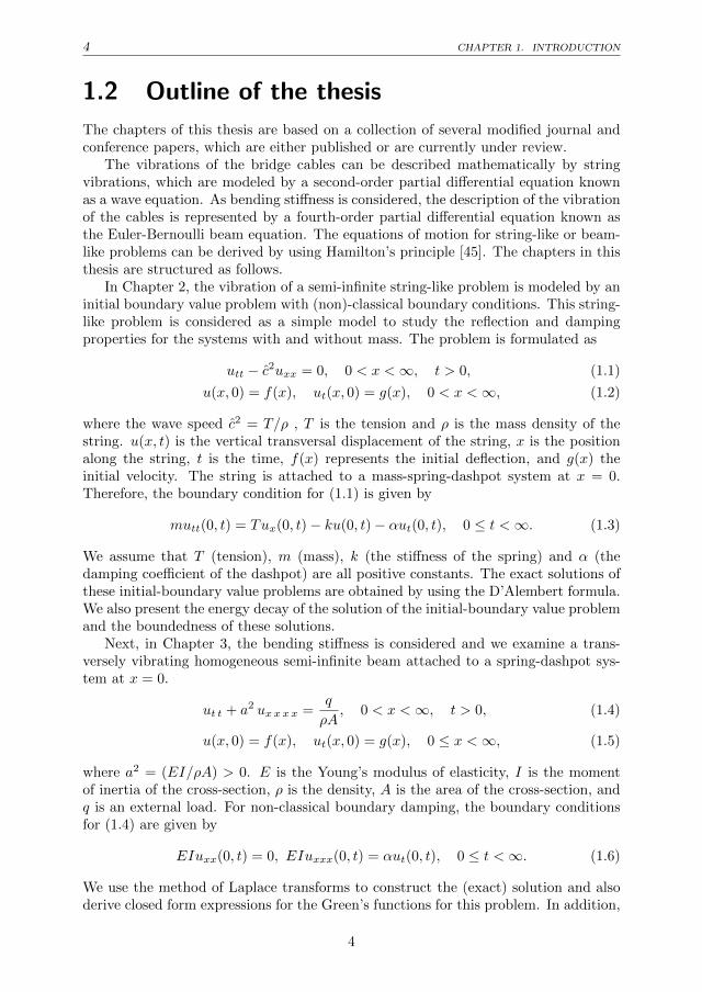
1.2 Outline of the thesis
The chapters of this thesis are based on a collection of several modified journal andconference papers, which are either published or are currently under review.
The vibrations of the bridge cables can be described mathematically by stringvibrations, which are modeled by a second-order partial differential equation knownas a wave equation. As bending stiffness is considered, the description of the vibrationof the cables is represented by a fourth-order partial differential equation known asthe Euler-Bernoulli beam equation. The equations of motion for string-like or beam-like problems can be derived by using Hamilton’s principle [45]. The chapters in thisthesis are structured as follows.
In Chapter 2, the vibration of a semi-infinite string-like problem is modeled by aninitial boundary value problem with (non)-classical boundary conditions. This string-like problem is considered as a simple model to study the reflection and dampingproperties for the systems with and without mass. The problem is formulated as
utt − c2uxx = 0, 0 < x <∞, t > 0, (1.1)
u(x, 0) = f(x), ut(x, 0) = g(x), 0 < x <∞, (1.2)
where the wave speed c2 = T/ρ , T is the tension and ρ is the mass density of thestring. u(x, t) is the vertical transversal displacement of the string, x is the positionalong the string, t is the time, f(x) represents the initial deflection, and g(x) theinitial velocity. The string is attached to a mass-spring-dashpot system at x = 0.Therefore, the boundary condition for (1.1) is given by
mutt(0, t) = Tux(0, t)− ku(0, t)− αut(0, t), 0 ≤ t <∞. (1.3)
We assume that T (tension), m (mass), k (the stiffness of the spring) and α (thedamping coefficient of the dashpot) are all positive constants. The exact solutions ofthese initial-boundary value problems are obtained by using the D’Alembert formula.We also present the energy decay of the solution of the initial-boundary value problemand the boundedness of these solutions.
Next, in Chapter 3, the bending stiffness is considered and we examine a trans-versely vibrating homogeneous semi-infinite beam attached to a spring-dashpot sys-tem at x = 0.
ut t + a2 ux x x x =q
ρA, 0 < x <∞, t > 0, (1.4)
u(x, 0) = f(x), ut(x, 0) = g(x), 0 ≤ x <∞, (1.5)
where a2 = (EI/ρA) > 0. E is the Young’s modulus of elasticity, I is the momentof inertia of the cross-section, ρ is the density, A is the area of the cross-section, andq is an external load. For non-classical boundary damping, the boundary conditionsfor (1.4) are given by
EIuxx(0, t) = 0, EIuxxx(0, t) = αut(0, t), 0 ≤ t <∞. (1.6)
We use the method of Laplace transforms to construct the (exact) solution and alsoderive closed form expressions for the Green’s functions for this problem. In addition,
4

1.2. OUTLINE OF THE THESIS 5
it is shown how waves are damped and reflected, and how much energy is dissipatedat the non-classical boundary.
Finally, in Chapter 4 the longitudinal and transversal in-plane vibrations of aninclined stretched beam with a time-varying mass, and in a uniform wind flow arestudied. While one end of the string (at x = 0) is fixed, a sliding damper is appliedat the other end of the beam (at x = L). The equations of motion describing thelongitudinal and transversal displacements of the tensioned Euler Bernoulli Beamcan be derived by using a variational principle [24]. The coupled system of partialdifferential equations to describe the in-plane displacements of the beam is reducedto a single partial differential equation by using Kirchhoff’s approach. We obtain
µvxxxx + vtt − vxx =ε[η10 + σ Ω1 cos(γ1x− Ω1t)
]vt (1.7)
− σ sin(γ1x− Ω1t)vtt + η2(1− x)vxx − η2vx
+ σ sin(γ1x− Ω1t)η3
, t > 0, 0 < x < 1,
with the boundary conditions
v(0, t; ε) = vxx(0, t; ε) = vx(1, t; ε) = 0, (1.8)
µvxxx(1, t; ε) = vx(1, t; ε) + ε[λvt(1, t; ε) + η2vx(1, t; ε)]. (1.9)
The stability of solutions is studied in detail by using the multiple-timescalesperturbation method.
5

6 CHAPTER 1. INTRODUCTION
6

Chapter 2Reflection and Damping Propertiesfor Semi-infinite String Equationswith Non-classical BoundaryConditions
Abstract. In order to answer the main question as indicated in the previous chapter,we should start to examine boundary reflection and damping properties of the string-like problem as a simple model. In this chapter, initial-boundary-value problems for alinear wave (string) equation are considered. The main objective is to study boundaryreflection and damping properties of waves in semi-infinite strings. This problem is ofconsiderable practical interest in the context of vibration suppression at boundariesof elastic structures. Solutions of wave equations will be constructed for two differentclasses of boundary conditions. In the first class, a massless system consisting ofa spring and damper will be considered at the boundary. In the second class, anadditional mass will be added to the system at the boundary. The D’Alembert methodwill be used to construct explicit solutions of the boundary value problem for theone-dimensional wave equation on the semi-infinite domain. It will also be shownhow waves are damped and reflected at these boundaries, and how much energy isdissipated at the boundary.
2.1 Introduction
Many researchers have paid considerable attention to the dynamics of mechanicalstructures due to rain, wind, earthquake, machines and traffic-induced vibrations.These vibrations in mechanical structures are of great importance because of their
Parts of this chapter have been published in [4] the Journal of Sound and Vibration 336 (2015)and as a contribution to the conference proceedings of ENOC 2014.
7

8CHAPTER 2. REFLECTION AND DAMPING PROPERTIES FOR SEMI-INFINITE STRING EQUATIONS
WITH NON-CLASSICAL BOUNDARY CONDITIONS
impact on our life. The motion of mechanical structures, such as for instance thevibrations of bridge cables and power transmission lines, can be described by math-ematical models which are wave-like or string-like problems [56, 18]. In order tosuppress the undesired oscillations of the mechanical structures, all kinds of damperscan be used at the boundary. Many dampers such as tuned mass dampers and oildampers have historically been used to reduce the wind-induced vibrations of tautcables to safe levels, and so to prevent fatigue failures of the structures.
In the literature there are some fundamental examples of classical boundary con-ditions without mass such as fixed and free end conditions [27]. More complicatedconditions for which the end point is connected to a spring and/or dashpot can befound in Graff [25] or in Morse and Feshbach [47]. In [25] the problem is solved byusing the Fourier transform method. In addition, by using the method of character-istics for one-dimensional wave equations, Morse and Feshbach [47] solved the sameproblem. In all of these cases no mass was attached to the system at the boundary.Moreover, it seems that a mass-spring-dashpot system attached at the boundary hasnot been treated analytically before in the literature. The main goal of this chapteris to investigate a linear equation for a semi-infinite string with and without massattached at the boundary. With our approach it is possible to compute directly forstring-like elastic structures the exact damping properties when a boundary damperis added to the structure. Depending on the choices of the parameter values of theboundary damper (i.e. mass, stiffness and damping parameters) the effectiveness canbe obtained exactly.
This chapter is organized as follows. In Section 2.2, we establish the governingequations of motion. In Section 2.3, we discuss variations on the relatively simplecase without mass, which arise in various physical problems. In other words, thestring is attached to a spring-dashpot system at x = 0 as shown in Figure. 2.1(a). Forthe more complicated conditions, in Section 2.4, we turn our attention to a spring-dashpot system with mass as shown in Figure 2.1(b). For both cases, we present notonly the energy decay of the solution of the initial-boundary value problem and theboundedness of these solutions, but also the reflection and damping properties of thesystem. Finally, in Section 2.5, we draw some conclusions.
2.2 The governing equations of motion
We will consider the perfectly flexible string on a semi-infinite interval. u(x, t) isthe vertical transversal displacement of the string, where x is the position along thestring, and t is the time. Let us assume that gravity and other external forces can beneglected. The equation of motion is for instance derived in reference [45], by usingHamilton’s principle:
u− c2u′′ = 0, 0 < x <∞, t > 0,
u(x, 0) = f(x), u(x, 0) = g(x), x > 0, (2.1)
where the wave speed c2 = T/ρ , T is the tension and ρ is the mass density of thestring. Here, f(x) and g(x) represent the initial displacement and initial velocity ofthe string, respectively. Note that the overdot (·) denotes the derivative with respectto time and the prime ()′ denotes the derivative with respect to the spatial variable
8

2.2. THE GOVERNING EQUATIONS OF MOTION 9
u
x
k
α
(a) The spring-dashpot system withoutmass
u
x
k
α
m
(b) The mass-spring-dashpot system
Figure 2.1: Two different physical models for an viscoelastic string.
x. As a boundary condition, (the spring-dashpot system) we have
Tu′(0, t) = ku(0, t) + αu(0, t), if m = 0, (2.2)
and for the mass-spring-dashpot system, we will have
mu(0, t) = Tu′(0, t)− ku(0, t)− αu(0, t), if m 6= 0. (2.3)
The wave travels between x = 0 and x = ∞ as shown in Figure 2.1(a) andFigure 2.1(b) It is assumed that m (mass), k (the stiffness of the spring) and α (thedamping coefficient of the dashpot) are all positive constants. In order to put theequation in a non-dimensional form the following dimensionless quantities are used:
u∗(x∗, t∗) =u(x, t)
L∗, x∗ =
x
L∗, t∗ =
t
T∗, f∗(x∗) =
f(x)
L∗, g∗(x∗) = g(x)
T∗L∗,
where L∗ and time T∗ are some dimensional characteristic quantities for the length andthe time respectively, and by inserting these non-dimensional quantities into Eq.(2.1),we obtain
u(x, t)− u′′(x, t) = 0, 0 < x <∞, t > 0, (2.4)
with initial conditions
u(x, 0) = f(x), u(x, 0) = g(x), 0 ≤ x <∞, (2.5)
and with boundary conditions
u′(0, t) = λu(0, t) + βu(0, t), t ≥ 0 (if m = 0), (2.6)
oru(0, t) = ηu′(0, t)− µu(0, t)− ψu(0, t), t ≥ 0 (if m 6= 0), (2.7)
9

10CHAPTER 2. REFLECTION AND DAMPING PROPERTIES FOR SEMI-INFINITE STRING EQUATIONS
WITH NON-CLASSICAL BOUNDARY CONDITIONS
where c2 = L2∗/T
2∗ , λ = k L∗/T , β = αL∗/T∗ T , η = T T 2
∗ /mL∗, µ = k T 2∗ /m
and ψ = αT∗/m. The asterisks indicating the dimensional quantities are omitted inEq.(2.4) through (2.7) and henceforth for convenience.
In order to examine the reflection of waves, we will consider u(x, 0) = f(x) andu(x, 0) = −f ′(x) as initial conditions, which implies that we initially only have wavestravelling to the left (i.e. travelling to the boundary at x = 0).
2.3 Reflection at boundaries
2.3.1 The spring-dashpot system (m = 0)
In this section, we will consider the case of a string of semi-infinite length, extending inthe positive direction from x = 0, where there is a support at x = 0 having transversestiffness force, and resistance. The initial-boundary value problem for u(x, t) is givenby
u(x, t)− u′′(x, t) = 0, 0 < x <∞, t > 0, (2.8)
u(x, 0) = f(x), u(x, 0) = g(x), 0 ≤ x <∞, (2.9)
u′(0, t) = λu(0, t) + βu(0, t), 0 ≤ t <∞, λ ≥ 0, β ≥ 0, (2.10)
where f ∈ C2, and g ∈ C1. It is well-known that the general solution of the one-dimensional wave equation is given by
u(x, t) = F (x− t) +G(x+ t). (2.11)
Here F and G functions represent propagating disturbances, and by using theinitial conditions, we obtain
F (x) =1
2f(x)− 1
2
∫ x
0
g(s) ds− K
2, (2.12)
G(x) =1
2f(x) +
1
2
∫ x
0
g(s) ds+K
2, (2.13)
where K is a constant of integration. Substitution of Eq.(2.12) and (2.13) into thegeneral solution Eq.(2.11) gives the well-known D’Alembert formula for u(x, t)
u(x, t) =1
2[f(x+ t) + f(x− t)] +
1
2
∫ x+t
x−tg(s) ds. (2.14)
For x− t < 0, f(x− t) is not yet defined in Eq.(2.14), and for x− t < s < 0, g(s)is not yet defined in Eq.(2.14). This “freedom” in f and in g will be used to satisfythe boundary condition Eq.(2.10). Substituting Eq.(2.14) into Eq.(2.10) yields:
f ′(−t)2− g(−t)
2+f ′(t)
2+g(t)
2=λ
[f(−t)
2+f(t)
2+
1
2
∫ t
−tg(s) ds
]+β
[−f′(−t)2
+g(−t)
2+f ′(t)
2+g(t)
2
], (2.15)
10
2.3. REFLECTION AT BOUNDARIES 11
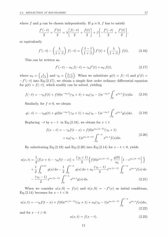
where f and g can be chosen independently. If g ≡ 0, f has to satisfy
f ′(−t)2
+f ′(t)
2= λ
[f(−t)
2+f(t)
2
]+ β
[−f′(−t)2
+f ′(t)
2
],
or equivalently
f ′(−t)−(
λ
1 + β
)f(−t) =
(β − 1
1 + β
)f ′(t) +
(λ
1 + β
)f(t). (2.16)
This can be written as,
f ′(−t)− κ0 f(−t) = γ0f′(t) + κ0 f(t), (2.17)
where κ0 =(
λ1+β
)and γ0 =
(β−11+β
). When we substitute y(t) = f(−t) and y′(t) =
−f ′(−t) into Eq.(2.17), we obtain a simple first order ordinary differential equationfor y(t) = f(−t), which readily can be solved, yielding
f(−t) = −γ0f(t) + f(0)e−κ0 t(γ0 + 1) + κ0(γ0 − 1)e−κ0 t
∫ t
0
eκ0 sf(s)ds. (2.18)
Similarly, for f ≡ 0, we obtain
g(−t) = −γ0g(t) + g(0)e−κ0 t(γ0 + 1) + κ0(γ0 − 1)e−κ0 t
∫ t
0
eκ0 sg(s)ds. (2.19)
Replacing −t by x− t in Eq.(2.18), we obtain for x < t
f(x− t) =− γ0f(t− x) + f(0)eκ0 (x−t)(γ0 + 1)
+ κ0(γ0 − 1)eκ0 (x−t)∫ t−x
0
eκ0 sf(s)ds.(2.20)
By substituting Eq.(2.19) and Eq.(2.20) into Eq.(2.14) for x− t < 0, yields
u(x, t) =1
2[f(x+ t)− γ0f(t− x)] +
(γ0 + 1)
2
f(0)eκ0 (x−t) +
g(0)
κ0
[1− eκ0 (x−t)
]+
1
2
∫ x+t
0
g(s) ds− 1
2
∫ t−x
0
g(s) ds+ κ0(γ0 − 1)
2eκ0 (x−t)
∫ t−x
0
eκ0 sf(s) ds
− (γ0 − 1)
2eκ0 (x−t)
∫ t−x
0
eκ0 sg(s) ds. (2.21)
When we consider u(x, 0) = f(x) and u(x, 0) = −f ′(x) as initial conditions,Eq.(2.14) becomes for x− t < 0:
u(x, t) = −γ0f(t− x) + f(0)eκ0 (x−t)(γ0 + 1) + κ0(γ0 − 1)eκ0 (x−t)∫ t−x
0
eκ0 sf(s)ds,
(2.22)and for x− t > 0:
u(x, t) = f(x− t). (2.23)
11

12CHAPTER 2. REFLECTION AND DAMPING PROPERTIES FOR SEMI-INFINITE STRING EQUATIONS
WITH NON-CLASSICAL BOUNDARY CONDITIONS
(a) β = 0 (b) λ = 0
Figure 2.2: The initial wave and its reflection.
Table 2.1 shows the extension of f(t) for negative arguments. As can be seen, thesolution has an odd or an even extension when we take β = 0, λ→∞ or β = 0, λ→ 0,respectively. Similarly, when we consider only damping at the boundary at x=0(λ = 0), the solution has again an odd or an even extension as β → ∞ or β → 0,respectively. We have ideal damping as β = 1, and λ = 0. Figure 2.2 also shows howa wave is reflected, that is, for f(x) = sin2(x) and g(x) = −f ′(x) for π < x < 2π, andf(x) = 0 elsewhere. Its reflection for x < 0 is plotted for different values of λ and β.
Table 2.1: Extension of f(t) for negative arguments when m = 0.
λ β extension of f(t) for the boundary condition
> 0 > 0 −γ0f(t) + f(0)e−κ0 t(γ0 − 1) + κ0(γ0 − 1)e−κ0 t∫ t0 eκ0 sf(s)ds,
where κ0 =(
λ1+β
)and γ0 =
(β−11+β
).
≥ 0 0 e−λ t f(0)− e−λ t∫ t0 eλ s[−f ′(s) + λ f(s)] ds=
f(t)− 2λ e−λ t∫ t0 eλ sf(s) ds=
−f(t) + 2e−λ tf(0) + 2e−λ t∫ t0 eλ s f ′(s) ds.
0 ≥ 0 1−β1+β
f(t) +(
2β1+β
)f(0).
12

2.3. REFLECTION AT BOUNDARIES 13
2.3.2 The mass-spring-dashpot system (m 6= 0)
In this section, a semi-infinite string with a mass added in the spring-dashpot systemat x = 0 is considered. We will determine the solution of
u(x, t)− u′′(x, t) = 0, 0 < x <∞, t > 0, (2.24)
u(x, 0) = f(x), u(x, 0) = g(x), 0 ≤ x <∞, (2.25)
u(0, t) = ηu′(0, t)− µu(0, t)− ψu(0, t), 0 ≤ t <∞, (2.26)
where η > 0, µ ≥ 0, ψ ≥ 0. We already know the general solution of the waveequation, and again by applying the boundary condition to Eq.(2.14), we obtain
f ′′(t) + f ′′(−t) + g′(t)− g′(−t) = η
[f ′(−t) + f ′(t)− g(−t) + g(t)
]− µ
[f(−t) + f(t) +
∫ t
−tg(s) ds
]− ψ
[−f ′(−t) + f ′(t) + g(t) + g(−t)
],
(2.27)
where f and g can be chosen independently. For g ≡ 0,
f ′′(−t)− (η + ψ)f ′(−t) + µ f(−t) = −f ′′(t) + (η − ψ)f ′(t)− µ f(t). (2.28)
We can rewrite Eq.(2.28) by putting the unknown function f(−t) = y(t), f ′(−t) =−y′(t), and f ′′(−t) = y′′(t). It then follows that
y′′(t) + θ y′(t) + µ y(t) = −f ′′(t) + (η − ψ)f ′(t)− µ f(t), (2.29)
where, θ = (η + ψ). Similarly, g(−t) can be obtained when f ≡ 0.The characteristic equation corresponding to Eq.(2.28) is given by
λ2 + θ λ+ µ = 0 ⇒ λ1,2 =−θ ±
√∆
2, (2.30)
where ∆ = θ2 − 4µ.Solving the characteristic equation will give two roots, λ1 and λ2. The behaviour
of the system depends on the relative values of the two fundamental parameters, µand θ. In particular, the qualitative behaviour of the system depends crucially onwhether the quadratic equation for λ has two real solutions, one real solution, or twocomplex conjugate solutions.
(i) The case ∆ > 0 or equivalently 4µ < θ2. There are two different real roots.The homogeneous solution is given by
yh(t) = b1eλ1t + b2eλ2t, (2.31)
where b1 and b2 are constants. When we apply the method of variations of parameters[9], we obtain the general solution of Eq.(2.28)
y(t) = b1 y1(t) + b2 y2(t) + Y (t), (2.32)
where y1(t) = eλ1t, y2(t) = eλ2t, and Y (t) is given by
Y (t) = −y1(t)
∫ t
0
y2(s)g(s)
W (y1, y2)ds+ y2(t)
∫ t
0
y1(s)g(s)
W (y1, y2)ds, (2.33)
13

14CHAPTER 2. REFLECTION AND DAMPING PROPERTIES FOR SEMI-INFINITE STRING EQUATIONS
WITH NON-CLASSICAL BOUNDARY CONDITIONS
in which the Wronskian W (y1, y2) is given by
W (y1, y2)(t) =
∣∣∣∣ eλ1t eλ2t
λ1eλ1t λ2eλ2t
∣∣∣∣ = (λ2 − λ1)e(λ1+λ2)t, (2.34)
and where g(s) = −f ′′(s) + (η − ψ)f ′(s)− µ f(s).Then,
Y (t) = − eλ1t
(λ2 − λ1)
∫ t
0
e−λ1s[−f ′′(s) + (η − ψ)f ′(s)− µ f(s)]ds
+eλ2t
(λ2 − λ1)
∫ t
0
e−λ2s[−f ′′(s) + (η − ψ)f ′(s)− µ f(s)]ds. (2.35)
By substituting Eq.(2.35) into the general solution Eq.(2.32) and by using inte-gration by parts, we obtain
y(t) =b1eλ1t + b2eλ2t − f(t) +f(0)
λ2 − λ1[eλ2t(λ2 − η + ψ)− eλ1t(λ1 − η + ψ)]
+f ′(0)
λ2 − λ1(eλ2t − eλ1t) +
eλ1t
λ1 − λ1(λ1
2 − λ1(η − ψ) + µ)
∫ t
0
e−λ1sf(s)ds
− eλ2t
λ2 − λ2(λ2
2 − λ2(η − ψ) + µ)
∫ t
0
e−λ2sf(s)ds.
(2.36)
In order to determine the constants b1 and b2, we take t = 0 and then it followsfrom y(0) = f(0) and y′(0) = −f ′(0) that
b1 =[−f ′(0)− λ2f(0)]
(λ1 − λ2)and b2 =
[−f ′(0)− λ1f(0)]
(λ2 − λ1). (2.37)
Hence,
f(−t) =− f(t) + f(0)
[(eλ1t + eλ2t) +
(η − ψ)
(λ2 − λ1)(eλ1t − eλ2t)
]+
eλ1t
(λ2 − λ1)
[(λ2
1 − λ1(η − ψ) + µ)
∫ t
0
e−λ1sf(s)ds
]− eλ2t
(λ2 − λ1)
[(λ2
2 − λ2(η − ψ) + µ)
∫ t
0
e−λ2sf(s)ds
]. (2.38)
(ii) The case ∆ = 0 or equivalently 4µ = θ2. There is a double root λ, whichis real. In this case, with only one root λ, the homogeneous solution of Eq.(2.29) isgiven by
yh(t) = (b3 + b4t)e−θt/2, (2.39)
where b3 and b4 are constants. Completely similar to the previous case, y(t) = f(−t)can be computed, yielding
f(−t) =− f(t) + f(0)e−θt/2[2 + t(ψ − η)] +
[θ(3η − ψ)
4+ µ
]e−θt/2
∫ t
0
s eθs/2f(s)ds
+
[2η − t
(θ(3η − ψ)
4+ µ
)]e−θt/2
∫ t
0
eθs/2f(s)ds. (2.40)
14
2.3. REFLECTION AT BOUNDARIES 15
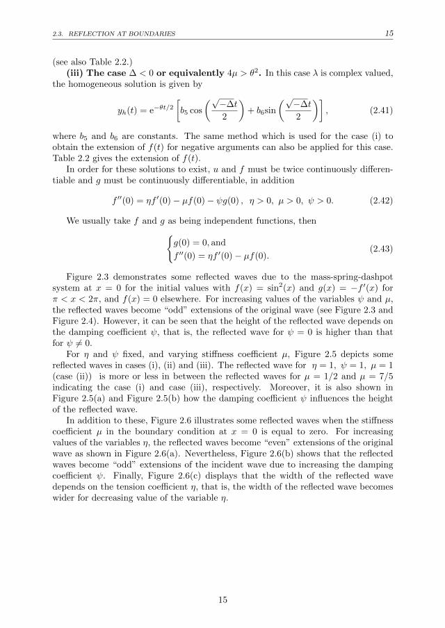
(see also Table 2.2.)(iii) The case ∆ < 0 or equivalently 4µ > θ2. In this case λ is complex valued,
the homogeneous solution is given by
yh(t) = e−θt/2[b5 cos
(√−∆t
2
)+ b6sin
(√−∆t
2
)], (2.41)
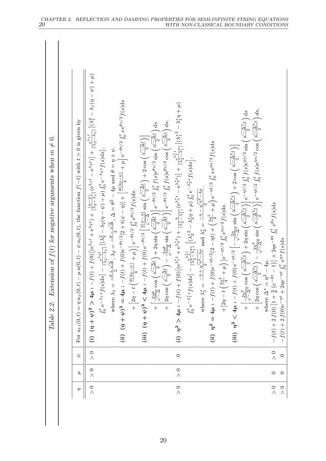
where b5 and b6 are constants. The same method which is used for the case (i) toobtain the extension of f(t) for negative arguments can also be applied for this case.Table 2.2 gives the extension of f(t).
In order for these solutions to exist, u and f must be twice continuously differen-tiable and g must be continuously differentiable, in addition
f ′′(0) = ηf ′(0)− µf(0)− ψg(0) , η > 0, µ > 0, ψ > 0. (2.42)
We usually take f and g as being independent functions, theng(0) = 0, and
f ′′(0) = ηf ′(0)− µf(0).(2.43)
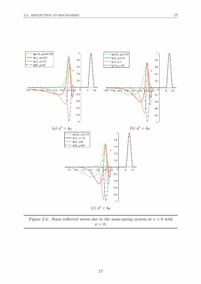
Figure 2.3 demonstrates some reflected waves due to the mass-spring-dashpotsystem at x = 0 for the initial values with f(x) = sin2(x) and g(x) = −f ′(x) forπ < x < 2π, and f(x) = 0 elsewhere. For increasing values of the variables ψ and µ,the reflected waves become “odd” extensions of the original wave (see Figure 2.3 andFigure 2.4). However, it can be seen that the height of the reflected wave depends onthe damping coefficient ψ, that is, the reflected wave for ψ = 0 is higher than thatfor ψ 6= 0.
For η and ψ fixed, and varying stiffness coefficient µ, Figure 2.5 depicts somereflected waves in cases (i), (ii) and (iii). The reflected wave for η = 1, ψ = 1, µ = 1(case (ii)) is more or less in between the reflected waves for µ = 1/2 and µ = 7/5indicating the case (i) and case (iii), respectively. Moreover, it is also shown inFigure 2.5(a) and Figure 2.5(b) how the damping coefficient ψ influences the heightof the reflected wave.
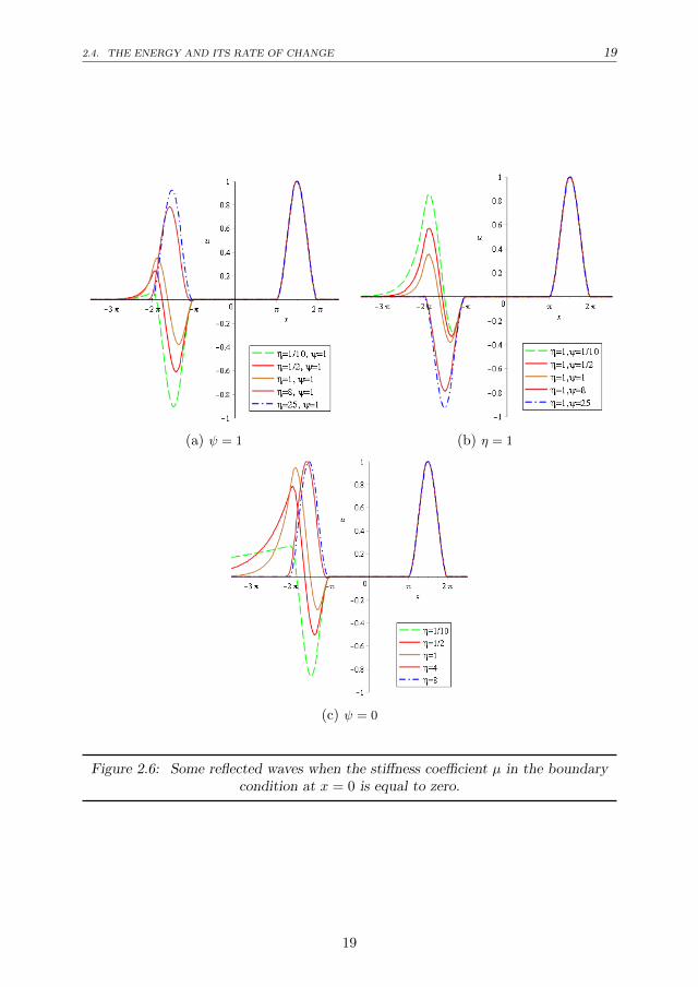
In addition to these, Figure 2.6 illustrates some reflected waves when the stiffnesscoefficient µ in the boundary condition at x = 0 is equal to zero. For increasingvalues of the variables η, the reflected waves become “even” extensions of the originalwave as shown in Figure 2.6(a). Nevertheless, Figure 2.6(b) shows that the reflectedwaves become “odd” extensions of the incident wave due to increasing the dampingcoefficient ψ. Finally, Figure 2.6(c) displays that the width of the reflected wavedepends on the tension coefficient η, that is, the width of the reflected wave becomeswider for decreasing value of the variable η.
15

16CHAPTER 2. REFLECTION AND DAMPING PROPERTIES FOR SEMI-INFINITE STRING EQUATIONS
WITH NON-CLASSICAL BOUNDARY CONDITIONS
(a) (η + ψ)2 > 4µ (b) (η + ψ)2 = 4µ
(c) (η + ψ)2 < 4µ
Figure 2.3: Some reflected waves due to the mass-spring-dashpot system at x = 0.
16
2.3. REFLECTION AT BOUNDARIES 17
(a) η2 > 4µ (b) η2 = 4µ
(c) η2 < 4µ
Figure 2.4: Some reflected waves due to the mass-spring system at x = 0 withψ = 0.
17

18CHAPTER 2. REFLECTION AND DAMPING PROPERTIES FOR SEMI-INFINITE STRING EQUATIONS
WITH NON-CLASSICAL BOUNDARY CONDITIONS
(a) η = ψ = 1, and varying µ (b) η = 1, ψ = 0, and varying µ
Figure 2.5: Some reflected waves for η and ψ fixed, and varying stiffness coefficientµ.
2.4 The energy and its rate of change
2.4.1 The energy and boundedness of solutions in the case m = 0
The total energy E(t) is the sum of the kinetic and the potential energies of the stringand the potential energy of the spring, that is
E(t) =1
2
∫ ∞0
(u2 + u′ 2)dx+λ
2u2(0, t). (2.44)
Taking the time derivative of E(t), we find
E(t) =
∫ ∞0
[u u+ u′ u′]dx+ λu(0, t) u(0, t),
by using integration by parts and by observing that there is no energy at x =∞, wededuce that
E(t) = −βu2(0, t). (2.45)
This implies that the energy E(t) decreases in time. Then,
E(t) = E(0)− β∫ t
0
u2(0, t)dt ≤ E(0), for all t ≥ 0. (2.46)
By using the Cauchy-Schwarz inequality, it then follows that
|u(x, t)| =∣∣∣∣∫ x
0
us(s, t)ds
∣∣∣∣ ≤√∫ ∞
0
u2s(s, t)ds ≤
√2E(t) ≤
√2E(0). (2.47)
18
2.4. THE ENERGY AND ITS RATE OF CHANGE 19
(a) ψ = 1 (b) η = 1
(c) ψ = 0
Figure 2.6: Some reflected waves when the stiffness coefficient µ in the boundarycondition at x = 0 is equal to zero.
19
20CHAPTER 2. REFLECTION AND DAMPING PROPERTIES FOR SEMI-INFINITE STRING EQUATIONS
WITH NON-CLASSICAL BOUNDARY CONDITIONS
Tab
le2.
2:E
xte
nsi
onoff
(t)
for
neg
ati
vearg
um
ents
wh
enm6=
0.
ηµ
ψF
orutt(0,t
)=ηux(0,t
)−µu
(0,t
)−ψut(0,t
),th
efu
nct
ionf
(−t)
wit
ht>
0is
giv
enby
>0
>0
>0
(i)
(η+ψ)2>
4µ
:−f
(t)
+f
(0)[ (e
λ1t
+eλ
2t)
+(η−ψ
)(λ
2−λ1)(eλ1t−
eλ2t)] +
eλ1t
(λ2−λ1)
[ (λ2 1−λ
1(η−ψ
)+µ
)∫ t 0
e−λ1sf
(s)ds] −
eλ2t
(λ2−λ1)
[ (λ2 2−λ
2(η−ψ
)+µ
)∫ t 0
e−λ2sf
(s)ds] ,
wh
ereλ
1=−θ
+√
∆2
,λ
2=−θ−√
∆2
,∆
=θ2−
4µ
an
dθ
=η
+ψ
.
(ii)
(η+ψ)2
=4µ
:−f
(t)
+f
(0)e−θt/
2[2
+t(ψ−η)]
+[ θ(3
η−ψ
)4
+µ] e−
θt/
2∫ t 0s
eθs/2f
(s)ds
+[ 2η−t( θ(3
η−ψ
)4
+µ)] e−
θt/
2∫ t 0
eθs/2f
(s)ds.
(iii)
(η+ψ)2<
4µ
:−f
(t)
+f
(0)e−θt/
2[ 2
(ψ−η)
√−
∆si
n( √ −
∆t
2
) +2
cos( √ −
∆t
2
)]+[ 2
ηθ
√−
∆co
s( √ −
∆t
2
) +2η
sin( √ −
∆t
2
)] e−θt/
2∫ t 0f
(s)eθs/2
sin( √ −
∆s
2
) ds
+[ 2η
cos( √ −
∆t
2
) −2ηθ
√−
∆si
n( √ −
∆t
2
)] e−θt/
2∫ t 0f
(s)eθs/2
cos( √ −
∆s
2
) ds.
>0
>0
0(i)η2>
4µ
:−f
(t)
+f
(0)[ (e
λ∗ 1t
+eλ∗ 2t)
+η
(λ∗ 2−λ∗ 1)(eλ∗ 1t−
eλ∗ 2t)] +
eλ∗ 1t
(λ∗ 2−λ∗ 1)
[ (λ∗ 1
2−λ∗ 1η
+µ
)
∫ t 0e−λ∗ 1sf
(s)ds] −
eλ∗ 2t
(λ∗ 2−λ∗ 1)
[ (λ∗ 2
2−λ∗ 2η
+µ
)∫ t 0
e−λ∗ 2sf
(s)ds] ,
wh
ereλ∗ 1
=−η
+√η2−
4µ
2an
dλ∗ 2
=−η−√η2−
4µ
2.
(ii)η2=
4µ
:−f
(t)
+f
(0)e−ηt/
2(2−ηt)
+( 3
η2
4+µ) e−
ηt/
2∫ t 0s
eηs/2f
(s)ds
+[ 2η−t( 3
η2
4+µ) ] e−
ηt/
2∫ t 0
eηs/2f
(s)ds.
(iii)η2<
4µ
:−f
(t)
+f
(0)e−ηt/
2[ −
2η
√−
∆∗
sin( √ −
∆∗t
2
) +2
cos( √ −
∆∗t
2
)]+[ 2
η2
√−
∆∗
cos( √ −
∆∗t
2
) +2η
sin( √ −
∆∗t
2
)] e−ηt/
2∫ t 0f
(s)eηs/2
sin( √ −
∆∗s
2
) ds
+[ 2η
cos( √ −
∆∗t
2
) −2η2
√−
∆∗
sin( √ −
∆∗t
2
)] e−ηt/
2∫ t 0f
(s)eηs/2
cos( √ −
∆∗s
2
) ds,
wh
ere
∆∗
=η
2−
4µ
.
>0
0>
0−f
(t)
+2f
(0)[ 1
+η θ
( e−θt−
1)] +
2ηe−θt∫ t 0
eθsf
(s)ds
>0
00
−f
(t)
+2f
(0)e−ηt
+2ηe−ηt∫ t 0
eηsf
(s)ds
20
2.4. THE ENERGY AND ITS RATE OF CHANGE 21
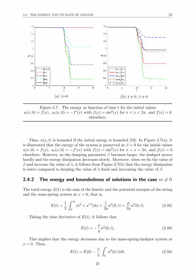
(a) λ=0 (b) λ 6= 0, β 6= 0
Figure 2.7: The energy as function of time t for the initial valuesu(x, 0) = f(x), ut(x, 0) = −f ′(x) with f(x) = sin2(x) for π < x < 2π, and f(x) = 0
elsewhere.
Thus, u(x, t) is bounded if the initial energy is bounded [19]. In Figure 2.7(a), itis illustrated that the energy of the system is preserved as β = 0 for the initial valuesu(x, 0) = f(x), ut(x, 0) = −f ′(x) with f(x) = sin2(x) for π < x < 2π, and f(x) = 0elsewhere. However, as the damping parameter β becomes larger, the dashpot moveshardly and the energy dissipation decreases slowly. Moreover, when we fix the value ofβ and increase the value of λ, it follows from Figure 2.7(b) that the energy dissipationis lower compared to keeping the value of λ fixed and increasing the value of β.
2.4.2 The energy and boundedness of solutions in the case m 6= 0
The total energy E(t) is the sum of the kinetic and the potential energies of the stringand the mass-spring system at x = 0, that is,
E(t) =1
2
∫ ∞0
(u2 + u′ 2)dx+1
2ηu2(0, t) +
µ
2ηu2(0, t). (2.48)
Taking the time derivative of E(t), it follows that
E(t) = −ψηu2(0, t). (2.49)
This implies that the energy decreases due to the mass-spring-dashpot system atx = 0. Then,
E(t) = E(0)− ψ
η
∫ t
0
u2(0, t)dt. (2.50)
21

22CHAPTER 2. REFLECTION AND DAMPING PROPERTIES FOR SEMI-INFINITE STRING EQUATIONS
WITH NON-CLASSICAL BOUNDARY CONDITIONS
(a) η = ψ = 1, and varying µ in E(t) (b) η = 1, and varying ψ, µ in the case (ii)
(c) ψ = 0 or ψ = 1, and varying η with µ=0
Figure 2.8: The energy as a function of time t due to (a-b) the mass-spring-daspothsystem and (c) the mass-daspoth system at x = 0 for the initial values
u(x, 0) = f(x), ut(x, 0) = −f ′(x) with f(x) = sin2(x) for π < x < 2π, and zeroelsewhere.
22

2.5. CONCLUSIONS 23
We already know from the previous section that u(x, t) is bounded if the initialenergy is bounded.
E(t) ≤ E(0), for all t ≥ 0. (2.51)
When the damping coefficient ψ > 0, it is obvious from Eq.(2.50) that energy ofthe system is dissipated. If ψ = 0, then E(t) = E(0), which expresses the conservationof energy.
Figure 2.8 shows the energy decay as a function of time t due to the mass-spring-daspoth system (see Figure 2.8(a) and Figure 2.8(b)) and the mass-daspoth system(see Figure 2.8(c)) at x = 0 for the initial values u(x, 0) = f(x), ut(x, 0) = −f ′(x)with f(x) = sin2(x) for π < x < 2π, and f(x) = 0 elsewhere. In Figure 2.8(a),it can be seen that at t = 9.7 the incident wave hits the boundary, and from thattime energy is dissipated. It follows that in case (iii) with µ = 7/5 more energy isdissipated than in case (i) with µ = 1/2 or in case (ii) with µ = 1.
For η fixed, and varying ψ and µ , Figure 2.8(b) demonstrates energy decay due tothe mass-spring-string system in the case (ii). It can be seen that energy of the systemis conserved when the damping coefficient ψ is equal to zero (see Figure 2.8(b) andFigure 2.8(c)). Furthermore, the energy decay becomes larger for increasing valuesof the coefficients ψ and µ. However, energy dissipation starts to become less forlarger values of the damping coefficient ψ (e.g. ψ = 2). Similarly, it follows fromFigure 2.8(c) that energy dissipation becomes less for parameter values of η largerthan 1.
2.5 Conclusions
In this chapter, an initial-boundary value problem for a wave equation on a semi-infinite interval has been studied. We applied the D’Alembert formula to obtain thegeneral solution for a one-dimensional wave equation, and examined the solution forvarious boundary conditions. This chapter provides an understanding of how wavesare damped and reflected by these boundaries, and how much energy is dissipatedat the boundary. It was also shown that the solution is bounded by using an energyintegral.
The results as given in this chapter can be used in several applications. For in-stance, in [17, 59, 60] the authors used the reflected waves due to a mass-less spring-dashpot boundary to study the vibrations of violin strings. Also these reflected waves(due to a mass-less spring dashpot) were used in [60] as approximations for the re-flected waves due to a mass-spring-dashpot boundary with nonzero mass. In thischapter we presented and computed the exact reflected waves. Part of the resultspresented in this chapter may be extended to axially moving strings, such as con-veyor belts, elevator cables, and so on, as well as to beam equations to compute thereflections of waves by these boundaries, but some modifications are needed.
23

24CHAPTER 2. REFLECTION AND DAMPING PROPERTIES FOR SEMI-INFINITE STRING EQUATIONS
WITH NON-CLASSICAL BOUNDARY CONDITIONS
24

Chapter 3On Constructing a Green’s Functionfor a Semi-Infinite Beam withBoundary Damping
Abstract. In the previous chapter, the boundary reflection and damping propertiesof waves in semi-infinite strings were studied. The vibrations of the bridge cablescan be described mathematically by string-like problem, which are modelled by asecond-order partial differential equation known as wave equation. However, themathematical model in Chapter 2 assumes that the bending stiffness is neglected andthis may not be the case for real world physical problems. In this chapter, the descrip-tion of the vibration of the cables is represented by a fourth-order partial differentialequation known as the Euler-Bernoulli beam equation. The main aim is to contributeto the construction of Green’s functions for initial boundary value problems for theEuler-Bernoulli beam equations. We consider a transversely vibrating homogeneoussemi-infinite beam with classical boundary conditions such as pinned, sliding, clampedor with non-classical boundary conditions such as dampers. This problem is of im-portant interest in the context of the foundation of exact solutions for semi-infinitebeams with boundary damping. The Green’s functions are explicitly given by usingthe method of Laplace transforms. The analytical results are validated by referencesand numerical methods. It is shown how the general solution for a semi-infinite beamequation with boundary damping can be constructed by the Green’s function method,and how damping properties can be obtained.
3.1 Introduction
In engineering, many problems describing mechanical vibrations in elastic structures,such as for instance the vibrations of power transmission lines [56] and bridge cables
Parts of this chapter have been published in [5] the Meccanica 52 (2016) and as a contributionto the conference proceedings of IUTAM 2015 and IMECE 2015.
25
26CHAPTER 3. ON CONSTRUCTING A GREEN’S FUNCTION FOR A SEMI-INFINITE BEAM WITH
BOUNDARY DAMPING
[44], can be mathematically represented by initial-boundary-value problems for a waveor a beam equation. Understanding the transverse vibrations of beams is important toprevent serious failures of the structures. In order to suppress the undesired vibrationsof the mechanical structures different kinds of dampers such as tuned mass dampersand oil dampers can be used at the boundary. Analysis of the transversally vibratingbeam problems with boundary damping is still of great interest today, and has beenexamined for a long time by many researchers [52, 29, 62]. In order to obtain a generalinsight into the over-all behavior of a solution, having a closed form expression whichrepresents a solution, can be very convenient. The Green’s function technique is oneof the few approaches to obtain integral representations for the solution [27].
In many papers and books, the vibrations of elastic beams have been studied byusing the Green’s function technique. A good overview can be found in e.g. [25, 26]and [55, 23, 27] for initial-value problems and for initial-boundary value problems,respectively. The initial-boundary value problem for a semi-infinite clamped bar hasalready been solved to obtain its Green’s function by using the method of Laplacetranforms [50]. To our best knowledge, we have not found any literature on the explicitconstruction of a Green’s function for semi-infinite beam with boundary damping.
The outline of the present chapter is as follows. In Section 3.2, we establish thegoverning equations of motion. The aim of this chapter is to give explicit formulafor the Green’s function for the following semi-infinite pinned, slided, clamped anddamped vibrating beams as listed in Table 3.1. In Section 3.3, we use the methodof Laplace transforms to construct the (exact) solution and also derive closed formexpressions for the Green’s functions for these problems. In Section 3.4, three classicalboundary conditions are considered and the Green’s functions for semi-infinite beamsare represented by definite integrals. For pinned and sliding vibrating beams, it isshown how the exact solution can be written with respect to even and odd extensionsof the Green’s function. In Section 3.5, we consider transversally vibrating elasticbeams with non-classical boundary conditions such as dampers. The analytical re-sults for semi-infinite beams in this case are compared with numerical results on abounded domain [0, L] with L large. The damping properties are given by the rootsof denominator part in the Laplace approach, or equivalently by the characteristicequation. Numerical and asymptotic approximations of the roots of a characteristicequation for the beam-like problem on a finite domain will be calculated. It will beshown how boundary damping can be effectively used to suppress the amplitudes ofoscillation. In Section 3.6, the concept of local energy storage is described. Finallysome conclusions will be drawn in Section 3.7.
3.2 The governing equations of motion
We will consider the transverse vibrations of a one-dimensional elastic Euler-Bernoullibeam which is infinitely long in one direction. The equations of motion can be derivedby using Hamilton’s principle [45]. The function u(x, t) is the vertical deflection ofthe beam, where x is the position along the beam, and t is the time. Let us assumethat gravity can be neglected. The equation describing the vertical displacement of
26
3.2. THE GOVERNING EQUATIONS OF MOTION 27
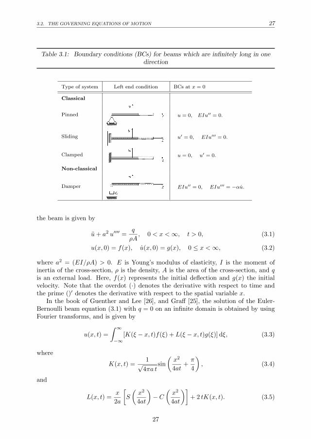
Table 3.1: Boundary conditions (BCs) for beams which are infinitely long in onedirection
Type of system Left end condition BCs at x = 0
Classical
Pinned u = 0, EIu′′ = 0.
Sliding u′ = 0, EIu′′′ = 0.
Clamped u = 0, u′ = 0.
Non-classical
Damper EIu′′ = 0, EIu′′′ = −αu.
the beam is given by
u+ a2 u′′′′ =q
ρA, 0 < x <∞, t > 0, (3.1)
u(x, 0) = f(x), u(x, 0) = g(x), 0 ≤ x <∞, (3.2)
where a2 = (EI/ρA) > 0. E is Young’s modulus of elasticity, I is the moment ofinertia of the cross-section, ρ is the density, A is the area of the cross-section, and qis an external load. Here, f(x) represents the initial deflection and g(x) the initialvelocity. Note that the overdot (·) denotes the derivative with respect to time andthe prime ()′ denotes the derivative with respect to the spatial variable x.
In the book of Guenther and Lee [26], and Graff [25], the solution of the Euler-Bernoulli beam equation (3.1) with q = 0 on an infinite domain is obtained by usingFourier transforms, and is given by
u(x, t) =
∫ ∞−∞
[K(ξ − x, t)f(ξ) + L(ξ − x, t)g(ξ)] dξ, (3.3)
where
K(x, t) =1√
4πa tsin
(x2
4at+π
4
), (3.4)
and
L(x, t) =x
2a
[S
(x2
4at
)− C
(x2
4at
)]+ 2 tK(x, t). (3.5)
27

28CHAPTER 3. ON CONSTRUCTING A GREEN’S FUNCTION FOR A SEMI-INFINITE BEAM WITH
BOUNDARY DAMPING
Here the functions C(z) and S(z) are the Fresnel integrals defined by
C(z) =
∫ z
0
cos(s)√s
ds, and S(z) =
∫ z
0
sin(s)√s
ds. (3.6)
In order to put the Eq. (3.1) and Eq. (3.2) in a non-dimensional form the followingdimensionless quantities are used:
u∗(x∗, t∗) =u(x, t)
L∗, x∗ =
x
L∗, t∗ =
κt
L∗, κ =
1
L∗
√EI
ρA,
f∗(x∗) =f(x)
L∗, g∗(x∗) =
g(x)
κ, q∗(x∗, t∗) =
q(x, t)ρAκ2
L∗,
where L∗ is the dimensional characteristic quantity for the length , and by insertingthese non-dimensional quantities into Eq. (3.1)-(3.2), we obtain the following initial-boundary value problem :
u(x, t) + u′′′′(x, t) = q(x, t), 0 < x <∞, t > 0, (3.7)
u(x,0) = f(x), u(x, 0) = g(x), 0 ≤ x <∞, (3.8)
and the boundary conditions at x = 0 are given in Table 3.1. The asterisks indicatingthe dimensional quantities are omitted in Eq. (3.7) and Eq. (3.8), and henceforth forconvenience.
In the coming sections, we will show how the Green’s functions for semi-infinitebeams with boundary conditions given at x = 0, can be obtained in explicit form.
3.3 The Laplace transform method
In this section, Green’s functions will be constructed by using the Laplace transformmethod in order to obtain an exact solution for the initial-boundary value problemEq. (3.7)-(3.8). Let us assume that the external force q(x, t) = δ(x − ξ) ⊗ δ(t) atthe point x = ξ at time t = 0, δ being Dirac’s function, and f(x) = g(x) = 0. TheGreen’s function Gξ(x, t), ξ > 0, expresses the displacements along the semi-infinitebeam.
We start by defining the Laplace operator as an integration with respect to thetime variable t. The Laplace transform gξ of Gξ with respect to t is defined as
gξ(x, p) = LGξ(x, t) =
∫ ∞0
e−ptGξ(x, t)dt, (3.9)
where gξ is the Green’s function of the differential operator L = (d4/dx4) + p2 on theinterval (0,∞). The Green’s function gξ satisfies the following properties [35]:
[G1] The Green’s function gξ satisfies the fourth order ordinary differential equa-tion in each of the two subintervals 0 < x < ξ and ξ < x <∞, that is, Lgξ = 0 exceptwhen x = ξ.
[G2] The Green’s function gξ satisfies at x = 0 one of the homogeneous boundaryconditions, as given in Table 3.1.
28
3.3. THE LAPLACE TRANSFORM METHOD 29
[G3] The Green’s function gξ and its first and second order derivatives exist andare continuous at x = ξ.
[G4] The third order derivative of the Green’s function gξ with respect to x hasa jump discontinuity which is defined as
limε→ 0
[g′′′ξ (ξ + ε)− g′′′ξ (ξ − ε)] = 1. (3.10)
The transverse displacement u(x, t) of the beam can be represented in terms ofthe Green’s function as (see also [51]):
u(x, t) = −∫ ∞
0
f(ξ) Gξ(x, t) dξ+
∫ ∞0
g(ξ)Gξ(x, t) dξ+
∫ t
0
∫ ∞0
q(ξ, τ)Gξ(x, t−τ)dξ dτ.
(3.11)
In the coming sections, we solve exactly the initial-boundary value problem for abeam on a semi-infinite interval for different types of boundary conditions.
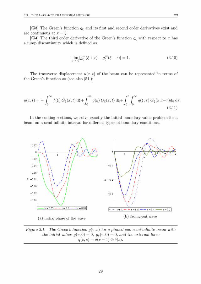
(a) initial phase of the wave(b) fading-out wave
Figure 3.1: The Green’s function g(v, s) for a pinned end semi-infinite beam withthe initial values g(v, 0) = 0, gs(v, 0) = 0, and the external force
q(v, s) = δ(v − 1)⊗ δ(s).
29

30CHAPTER 3. ON CONSTRUCTING A GREEN’S FUNCTION FOR A SEMI-INFINITE BEAM WITH
BOUNDARY DAMPING
(a) initial phase of the wave (b) fading-out wave
Figure 3.2: The Green’s function g(v, s) for a sliding end semi-infinite beam withthe initial values g(v, 0) = 0, gs(v, 0) = 0, and the external force
q(v, s) = δ(v − 1)⊗ δ(s).
3.4 Classical boundary conditions
3.4.1 Pinned end: u(0, t) = u′′(0, t) = 0
In this section, we consider a semi-infinite beam equation, when the displacement andthe bending moment are specified at x = 0, i.e. u(0, t) = u′′(0, t) = 0, and when thebeam has an infinite extension in the positive x-direction. By using the requirements[G1]-[G4], gξ is uniquely determined, and we obtain
gξ =1
8β3
e−β|x−ξ|[cosβ(x− ξ) + sinβ|x− ξ|] (3.12)
+ e−β(x+ξ)[−cosβ(x+ ξ)− sinβ(x+ ξ)],
where β2 = p/2. In order to invert the Laplace transform, we use the formula (see[15], page 93)
L−1[(√p2)−1φ(
√p2)]
=
∫ t
0
L−1φ(τ) dτ, (3.13)
and (see [48], page 279)
L−1[p−1/2e−
√pzcos(
√pz)]
=1√πt
cos( z
2t
), (3.14)
L−1[p−1/2e−
√pzsin(
√pz)]
=1√πt
sin( z
2t
), (3.15)
30

3.4. CLASSICAL BOUNDARY CONDITIONS 31
where z = |x±ξ|√2
. The Green’s function yields
Gξ(x, t) = −∫ t
0
[K(ξ − x, τ)−K(ξ + x, τ)] dτ, (3.16)
where the kernel function is defined by
K(x, τ) =1√4πτ
sin
(x2
4τ+π
4
). (3.17)
When we assume for Eq. (3.7) and Eq. (3.8) that the external loading is absent(q = 0), and that the initial displacement f(x) and the initial velocity g(x) arenonzero, one can find the solution of the pinned end semi-infinite beam in the formof Eq. (3.3) as
u(x, t) =
∫ ∞0
[[K(ξ−x, t)−K(ξ+x, t)]f(ξ)+[L(ξ−x, t)−L(ξ+x, t)]g(ξ)
]dξ, (3.18)
where K and L are given by Eq. (3.4) and Eq. (3.5). It should be observed thatEq. (3.18) could have been obtained by using Eq. (3.3) and the boundary conditionsu = u′′ = 0 at x = 0. From which it simply follows that f and g should be extendedas odd functions in their argument, and then by simplifying the so-obtained integral,one obtains Eq. (3.18).
On the other hand, when we consider that the external loading is nonzero, forexample, q = δ(x − ξ) ⊗ δ(t), and the initial disturbances are zero (f = g = 0), thesolution of pinned end semi-infinite beam can be written in a non-dimensional form.By substituting the following dimensionless quantities in Eq. (3.16)
v =x
ξ, s =
t
ξ2, σ =
t
τ, g(v, s) =
Gξξ. (3.19)
We obtain
g(v, s) = −√
s
4π
∫ ∞1
[sin
(σ(v − 1)2
4s+π
4
)− sin
(σ(v + 1)2
4s+π
4
)]dσ
σ3/2. (3.20)
Figure 3.1 shows the shape of the semi-infinite one-sided pinned beam during itsoscillation. It can be observed how the amplitude of the impulse at x = ξ is increasingand how the deflection curves start to develop rapidly from the boundary at x = 0 asnew time variable s is increasing, where s is given by Eq. (3.19).
3.4.2 Sliding end: u′(0, t) = u′′′(0, t) = 0
In this section, we consider a semi-infinite beam equation for x > 0, when the bendingslope and the shear force are specified at x = 0, i.e. u′(0, t) = u′′′(0, t) = 0. The samemethod which is used in Section 3.4.1 to obtain the Green’s function can also beapplied for the sliding end semi-infinite beam. The Green’s function is given by
Gξ(x, t) =
∫ t
0
[K(ξ − x, τ) +K(ξ + x, τ)] dτ, (3.21)
31
32CHAPTER 3. ON CONSTRUCTING A GREEN’S FUNCTION FOR A SEMI-INFINITE BEAM WITH
BOUNDARY DAMPING
and the transverse displacement u(x, t) of the beam without an external loading isgiven by
u(x, t) =
∫ ∞0
[[K(ξ−x, t)+K(ξ+x, t)]f(ξ)+[L(ξ−x, t)+L(ξ+x, t)]g(ξ)
]dξ. (3.22)
Eq. (3.22) also could have been obtained by using Eq. (3.3) and the boundaryconditions u′ = u′′′ = 0 at x = 0. It follows that f and g should be extended aseven functions in their argument, and then by simplifying the so-obtained integral,we obtain Eq. (3.22). By using the same dimensionless quantities as in Section 3.4.1,the non-dimensional form of the solution for the sliding end semi-infinite beam isgiven by:
g(v, s) = −√
s
4π
∫ ∞1
[sin
(σ(v − 1)2
4s+π
4
)+ sin
(σ(v + 1)2
4s+π
4
)]dσ
σ3/2. (3.23)
Similarly, Figure 3.2 demonstrates the shape of the semi-infinite one-sided slidingbeam during its oscillation. It can be seen how the amplitude of the impulse at x = ξis increasing and how the deflection curve is developing from the boundary at x = 0as the new time variable s is increasing.
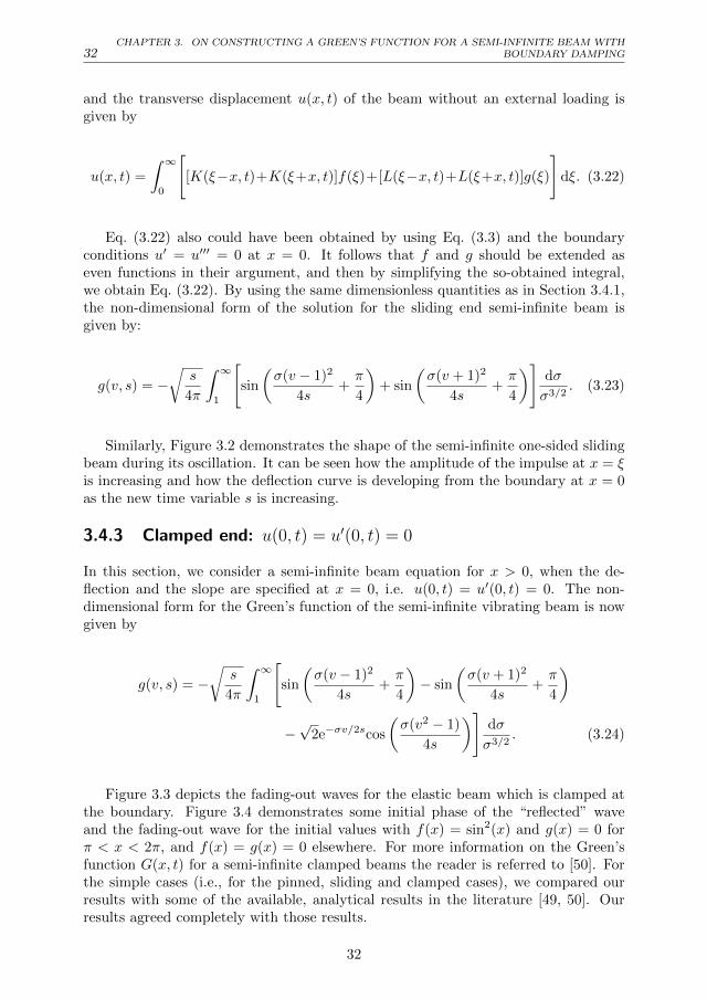
3.4.3 Clamped end: u(0, t) = u′(0, t) = 0
In this section, we consider a semi-infinite beam equation for x > 0, when the de-flection and the slope are specified at x = 0, i.e. u(0, t) = u′(0, t) = 0. The non-dimensional form for the Green’s function of the semi-infinite vibrating beam is nowgiven by
g(v, s) = −√
s
4π
∫ ∞1
[sin
(σ(v − 1)2
4s+π
4
)− sin
(σ(v + 1)2
4s+π
4
)
−√
2e−σv/2scos
(σ(v2 − 1)
4s
)]dσ
σ3/2. (3.24)
Figure 3.3 depicts the fading-out waves for the elastic beam which is clamped atthe boundary. Figure 3.4 demonstrates some initial phase of the “reflected” waveand the fading-out wave for the initial values with f(x) = sin2(x) and g(x) = 0 forπ < x < 2π, and f(x) = g(x) = 0 elsewhere. For more information on the Green’sfunction G(x, t) for a semi-infinite clamped beams the reader is referred to [50]. Forthe simple cases (i.e., for the pinned, sliding and clamped cases), we compared ourresults with some of the available, analytical results in the literature [49, 50]. Ourresults agreed completely with those results.
32
3.5. NON-CLASSICAL BOUNDARY CONDITIONS 33
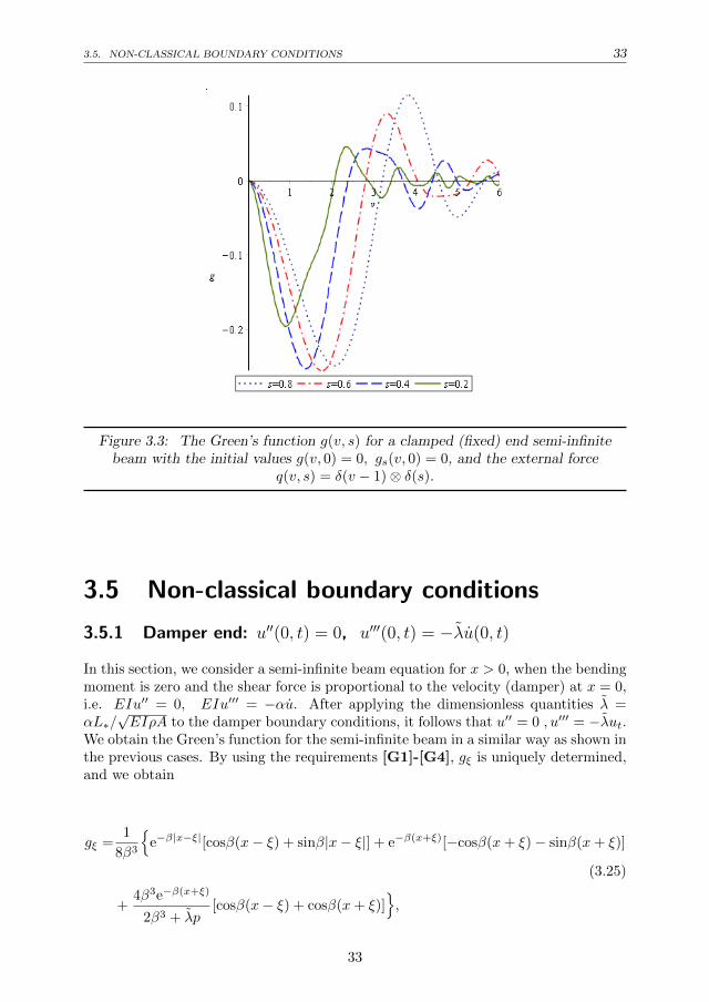
Figure 3.3: The Green’s function g(v, s) for a clamped (fixed) end semi-infinitebeam with the initial values g(v, 0) = 0, gs(v, 0) = 0, and the external force
q(v, s) = δ(v − 1)⊗ δ(s).
3.5 Non-classical boundary conditions
3.5.1 Damper end: u′′(0, t) = 0, u′′′(0, t) = −λu(0, t)
In this section, we consider a semi-infinite beam equation for x > 0, when the bendingmoment is zero and the shear force is proportional to the velocity (damper) at x = 0,i.e. EIu′′ = 0, EIu′′′ = −αu. After applying the dimensionless quantities λ =αL∗/
√EIρA to the damper boundary conditions, it follows that u′′ = 0 , u′′′ = −λut.
We obtain the Green’s function for the semi-infinite beam in a similar way as shown inthe previous cases. By using the requirements [G1]-[G4], gξ is uniquely determined,and we obtain
gξ =1
8β3
e−β|x−ξ|[cosβ(x− ξ) + sinβ|x− ξ|] + e−β(x+ξ)[−cosβ(x+ ξ)− sinβ(x+ ξ)]
(3.25)
+4β3e−β(x+ξ)
2β3 + λp[cosβ(x− ξ) + cosβ(x+ ξ)]
,
33

34CHAPTER 3. ON CONSTRUCTING A GREEN’S FUNCTION FOR A SEMI-INFINITE BEAM WITH
BOUNDARY DAMPING
where β2 = p/2. In order to invert the Laplace transform, we use the formula (see[15], page 93)
L−1[p−1φ(p)
]=
∫ t
0
L−1φ(τ)dτ. (3.26)
(a) pinned beam (b) sliding beam
(c) clamped beam
Figure 3.4: Some reflected waves for a semi-infinite one-sided beam withf(x) = sin2(x) and g(x) = 0 for π < x < 2π, and f(x) = 0 elsewhere.
Here
34

3.5. NON-CLASSICAL BOUNDARY CONDITIONS 35
Figure 3.5: The Green’s function g(v, s) for a semi-infinite beam with boundarydamping (λ = 1) for the initial values g(v, 0) = 0, gs(v, 0) = 0, and the external
force q(v, s) = δ(v − 1)⊗ δ(s).
φ(p) =p−1/2
2√
2e−√pη[cos(
√pη) + sin(
√pη)]− p−1/2
2√
2e−√pµ[cos(
√pµ) + sin(
√pµ)]
(3.27)
+p−1/2
2√
2e−√pµ 2p3/2
p3/2 +√
2λp[cos(
√pη) + cos(
√pµ)],
where η = (x+ξ)√2
and µ = |x−ξ|√2
. In Eq. (3.27), we use Eq. (3.14)-(3.15) for the first
two terms, and the following convolution theorem for the last term (see [15], page 92)
L−1 [φ1(p) φ2(p)] = f1(t) ∗ f2(t) =
∫ t
0
f1(r)f2(t− r)dr, (3.28)
where
φ1(p) =p−1/2
2√
2[cos(
√pη) + cos(
√pµ)], (3.29)
φ2(p) = e−√pµ 2p3/2
p3/2 +√
2λp. (3.30)
35

36CHAPTER 3. ON CONSTRUCTING A GREEN’S FUNCTION FOR A SEMI-INFINITE BEAM WITH
BOUNDARY DAMPING
For the inverse Laplace transform of Eq. (3.29), we use the following formula (see[12], page 106)
L−1[p−1/2cos(
√pη)]
=1√πt
sin( η
4t+π
4
), (3.31)
and for the inverse Laplace transform of Eq. (3.30), we use the following formulas (see[7], page 245-246)
L−1[e−√pµ]
=
õ
2√πt−3/2e−µ/4t,Re(µ) > 0, (3.32)
L−1
[e−µ√p
√p+ λ
√2
]=
e−µ2/4t
√πt− λ√
2eµλ√
2+2λ2t erfc
(µ
2√t
+ λ√
2t
), (3.33)
where the error function is defined as
erfc(x) =2√π
∫ ∞x
e−t2
dt. (3.34)
Then, the Green’s function is given by
Figure 3.6: The Green’s function g(v, s) for a semi-infinite beam with differentboundary damping parameters for the initial values g(v, 0) = 0, gs(v, 0) = 0, and
the external force q(v, s) = δ(v − 1)⊗ δ(s) at s = 0.8.
36

3.5. NON-CLASSICAL BOUNDARY CONDITIONS 37
Gξ(x, t) =−∫ t
0
1
2√πτ
[sin
((x− ξ)2
4τ+π
4
)− sin
((x+ ξ)2
4τ+π
4
)]dτ
−∫ t
0
∫ τ
0
[sin
((x− ξ)2
8(τ − r)+π
4
)+ sin
((x+ ξ)2
8(τ − r)+π
4
)][
e−(x+ξ)2/8r (x+ ξ − 4λr)
4πr√r(τ − r)
+2λ2√
2π(τ − r)eλ(x+ξ)+2λ2r
erfc
((x+ ξ + 4λr)
2√
2r
)]drdτ. (3.35)
When we assume that the external loading is nonzero, for example, q(x, t) = δ(x−ξ)⊗ δ(t), and the initial disturbances are zero (u(x, 0) = f(x) = 0, u(x, 0) = g(x) =0), the solution for the semi-infinite beam with damping boundary can be writtenin a non-dimensional form by substituting the following dimensionless quantities inEq. (3.5.1):
v =x
ξ, s =
t
ξ2, s =
τ
ξ2, σ =
t
τ, ϕ =
τ
r, λ =
λ
ξ, g(v, s) =
Gξξ,
we obtain
g(v, s) =−∫ ∞
1
√s
2√πσ3
[sin
((v − 1)2σ
4s+π
4
)− sin
((v + 1)2σ
4s+π
4
)]dσ
−∫ ∞
1
∫ ∞1
[sin
(σϕ(v − 1)2
8s(ϕ− 1)+π
4
)+ sin
(σϕ(v + 1)2
8s(ϕ− 1)+π
4
)][
e−σϕ(v+1)2/8s
(σϕ(v + 1)− 4λs
4πσ2ϕ√ϕ− 1
)+
λ2√
2s3√πσ5ϕ3(ϕ− 1)
eλ(v+1)+ 2λ2sσϕ
erfc
(σϕ(v + 1) + 4λs
2√
2sσϕ
)]dϕdσ. (3.36)
Figure 3.5 shows the shape for the semi-infinite beam with boundary dampingduring its oscillation. It is observed how the vibration is suppressed due to using adamper (λ = 1) at the boundary x = 0. Figure 3.6 depicts the Green’s function of thesemi-infinite beam for varying boundary damping parameters λ at s = 0.8. As can beseen, the damping boundary condition starts to behave like free and pinned boundarycondition when we take λ → 0 and λ → ∞, respectively. For the damping case, wecompare our solution in the next section with a long bounded beam by applying theLaplace transform method for a certain value of λ.
37

38CHAPTER 3. ON CONSTRUCTING A GREEN’S FUNCTION FOR A SEMI-INFINITE BEAM WITH
BOUNDARY DAMPING
3.5.2 Damper-clamped end: u′′′(0, t) = −λu(0, t), u′′(0, t) = 0, u(L, t) =0, u′(L, t) = 0
In this section, we compare our semi-infinite results with results for a bounded domain[0, L] with L large. We can formulate the dimensionless initial boundary value problemdescribing the transverse vibrations of a damped horizontal beam which is attachedto a damper at x = 0 as follows:
u(x, t) + u′′′′(x, t) = q(x, t), 0 < x < L, t > 0, (3.37)
u(x, 0) = f(x), u(x, 0) = g(x), 0 ≤ x < L, (3.38)
and boundary conditions,
u′′′(0, t) = −λu(0, t), u′′(0, t) = 0, t ≥ 0, (3.39)
u(L, t) = 0, u′(L, t) = 0, t ≥ 0.
We will also solve this problem by using the Laplace transform method whichreduces the partial differential equation Eq. (3.68) to a non-homogeneous linear ordi-nary differential equation, which can be solved by using standard techniques [20, 28].When we apply the Laplace transform method, which was defined in Eq. (3.9), toEqs. (3.68)-(3.70), we obtain the following boundary value problem
PDE: U ′′′′(x, p) + p2U(x, p) = Q(x, p), (3.40)
BCs: U ′′′(0, p) = −λ[ p U(0, p)− f(0)], (3.41)
U ′′(0, t) = U(L, p) = U ′(L, p) = 0,
where U(x, p) and Q(x, p) are the Laplace transforms of u(x, t) and q(x, t), and p isthe transform variable. Here, Q(x, p) = δ(x− ξ)+p u(x, 0)+ u(x, 0). We assume thatthe initial conditions are zero, that is u(x, 0) = f(x) = 0 and u(x, 0) = g(x) = 0.
The general solution of the homogeneous equation, that is, Eq. (3.71) withQ(x, p) =0, is given by
U(x, β) = C1(β)cos(βx) + C2(β)sin(βx) + C3(β)cosh(βx) + C4(β)sinh(βx), (3.42)
where Cj(β) are arbitrary functions for j = 1..4. For simplicity, we consider p2 = −β4,so that p = ∓iβ2. We consider only the case p = iβ2 for further calculations, becausethe case p = −iβ2 will also lead to the same p. The particular solution of the non-homogeneous equation Eq. (3.71) can be defined by using the method of variation ofparameters. We rewrite the general solution as follows:
U(x, β) =K1(β)cos(βx) +K2(β)sin(βx) +K3(β)cosh(βx) +K4(β)sinh(βx)
+1
2β3
∫ x
0
Q(s, β)[sin(β(s− x))− sinh(β(s− x))]ds, (3.43)
where Q(s, β) = δ(s− ξ). Kj(β) for j = 1..4 can be determined from the boundaryconditions and the solution of Eq. (3.71) and Eq. (3.72) is given by
U(x, β) =
∫ L
0
Q(s, β)H1(s, β : x)ds+
∫ x
0
Q(s, β)H2(s, β : x)ds, (3.44)
38
3.5. NON-CLASSICAL BOUNDARY CONDITIONS 39
(a) The first ten oscillation modes asapproximation of the solution of u(x, t) for a
damper-clamped ended finite beam
(b) The first forty oscillation modes asapproximation of the solution of u(x, t) for a
damper-clamped ended finite beam
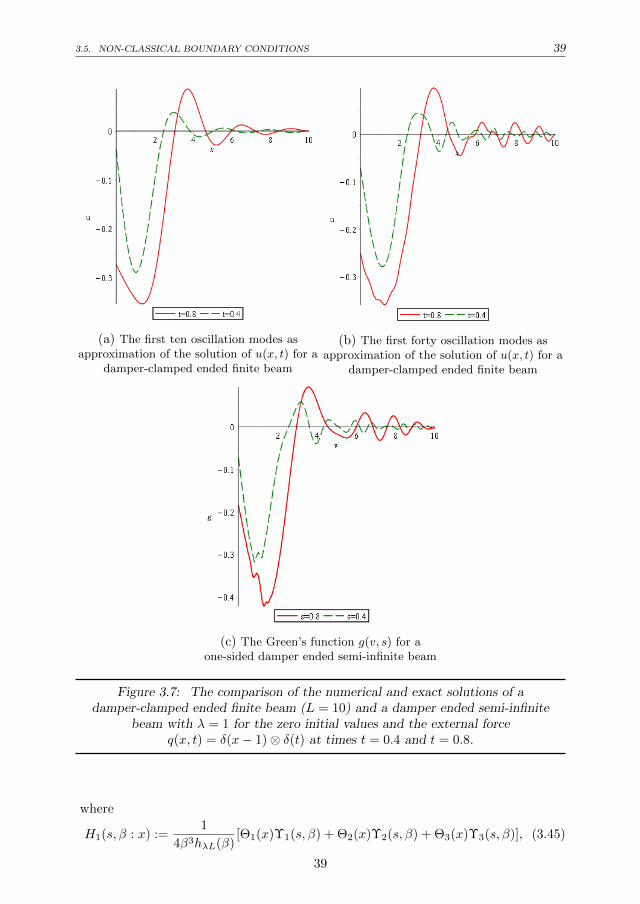
(c) The Green’s function g(v, s) for aone-sided damper ended semi-infinite beam
Figure 3.7: The comparison of the numerical and exact solutions of adamper-clamped ended finite beam (L = 10) and a damper ended semi-infinite
beam with λ = 1 for the zero initial values and the external forceq(x, t) = δ(x− 1)⊗ δ(t) at times t = 0.4 and t = 0.8.
where
H1(s, β : x) :=1
4β3hλL(β)[Θ1(x)Υ1(s, β) + Θ2(x)Υ2(s, β) + Θ3(x)Υ3(s, β)], (3.45)
39

40CHAPTER 3. ON CONSTRUCTING A GREEN’S FUNCTION FOR A SEMI-INFINITE BEAM WITH
BOUNDARY DAMPING
Θ1(x) := cos(βx) + cosh(βx), (3.46)
Υ1(s, β) :=[sin(β(L− s))− sinh(β(L− s))]β[cos(βL) + cosh(βL)]
−[cos(β(L− s))− cosh(β(L− s))]β[sin(βL) + sinh(βL)], (3.47)
Θ2(x) := sin(βx), (3.48)
Υ2(s, β) :=[sin(β(L− s))− sinh(β(L− s))][2λicosh(βL)
+β(sin(βL)− sinh(βL))]− [cos(β(L− s))− cosh(β(L− s))][2λisinh(βL)− β(cos(βL) + cosh(βL))], (3.49)
Θ3(x) := sinh(βx), (3.50)
Υ3(s, β) :=[sin(β(L− s))− sinh(β(L− s))][2λicos(βL)
−β(sin(βL)− sinh(βL))]− [cos(β(L− s))− cosh(β(L− s))][2λisin(βL) + β(cos(βL) + cosh(βL))], (3.51)
hλL(β) := β[1 + cos(βL)cosh(βL)] + λi[cosh(βL)sin(βL)− sinh(βL)cos(βL)], (3.52)
H2(s, β : x) :=1
2β3[sin(β(s− x))− sinh(β(s− x))]. (3.53)
In order to obtain the solution of Eqs. (3.68)-(3.70), the inverse Laplace transformof U(x, p) will be applied by using Cauchy’s residue theorem, that is,
u(x, t) =1
2πi
∫ γ+i∞
γ−i∞eptU(x, p)dp =
∑n
Res(eptU(x, p), p = pn), (3.54)
for γ > 0. Here Res(eptU(x, p), p = pn) is the residue of eptU(x, p) at the isolatedsingularity at p = pn. The poles of U(x, p) are determined by the roots of the followingcharacteristic equation
hλL(β) := 0, (3.55)
which is a “transcendental equation” defined in Eq. (3.5.2). The zeros of hλL(β) forλ = 0, which reduces the problem to the clamped-free beam, have been consideredin [36]. By using Rouche’s theorem, it can be shown that the number of roots ofhλL(β) := 0 (λ > 0) is equal to the same number of roots of hL(β) := 0 (λ = 0).For the proof of Rouche’s theorem, the reader is refered to Ref. [16]. Eq. (3.55) hasinfinitely many roots [46]. By using the relation p = iβ2, we can determine the roots
40

3.5. NON-CLASSICAL BOUNDARY CONDITIONS 41
of p, which are defined in complex conjugate pairs, such that pn = pren ∓ ipimn , wheren ∈ N and pren , p
imn ∈ R. So, the damping rate and oscillation rate are given by
pren := −2βren βimn and pimn := (βren )2 − (βimn )2, respectively.
In order to construct asymptotic approximations of the roots of hλL(β), we firstmultiply Eq. (3.55) by L, and define β = βL and λ = λL. Hence, we obtain
hλ(β) ≡ β[1 + cos(β)cosh(β)] + λi[cosh(β)sin(β)− sinh(β)cos(β)] = 0. (3.56)
Table 3.2: Numerical approximations of the solutions βn and pn of thecharacteristic equation Eq. (3.55) for the case L = 10 and λ = 1.
n βnum,n pnum,n (n− 12
) πL
-1 0.03887+0.03887i -0.00302+0i -
0 1.00000+1.00000i -2.00000+0i -
1 - - 0.15708
2 0.39535+0.01861i -0.01471+0.15596i 0.47124
3 0.71834+0.03367i -0.04837+0.51488i 0.78540
4 1.04526+0.04286i -0.08960+1.09073i 1.09956
5 1.37292+0.04574i -0.12560+1.88282i 1.41372
6 1.69789+0.04416i -0.14996+2.88088i 1.72788
7 2.01967+0.04084i -0.16497+4.07740i 2.04204
8 2.33906+0.03727i -0.17435+5.46981i 2.35619
9 2.65687+0.03395i -0.18040+7.05781i 2.67035
10 2.97365+0.03104i -0.18460+8.84163i 2.98451
11 3.28974+0.02850i -0.18752+10.82158i 3.39867
12 3.60537+0.02631i -0.18971+12.99800i 3.61283
13 3.92066+0.02440i -0.19133+15.37098i 3.92699
14 4.23571+0.02274i -0.19264+17.94072i 4.24115
15 4.55059+0.02127i -0.19358+20.70742i 4.55531
16 4.86533+0.01998i -0.19442+23.67104i 4.86947
17 5.17997+0.01883i -0.19508+26.83173i 5.18363
18 5.49453+0.01780i -0.19561+30.18954i 5.49779
19 5.80903+0.01688i -0.19611+33.74454i 5.81195
20 6.12348+0.01605i -0.19656+37.49675i 6.12611
41

42CHAPTER 3. ON CONSTRUCTING A GREEN’S FUNCTION FOR A SEMI-INFINITE BEAM WITH
BOUNDARY DAMPING
Next, multiplying hλ(β) by (2)/(β eβ), the characteristic equation yields
cos(β) = O(|β|−2) + i
(λ
β[cos(β)− sin(β)] +O(|β|−3)
), (3.57)
or
cos(β) = O(|β|−1), (3.58)
which is valid in a small neighbourhood of k = (n− 12 ) for all n > 0. After applying
Rouche’s theorem (see [22]), the following asymptotic solutions for βn and pn areobtained
βn = ∓ 1
L
[kπ +O(|n|−2) + i
(λL
kπ+O(|n|−2)
)], (3.59)
pn =−2λ
L+O(|n|−1) + i
((kπ)4 − (λL)2
(kLπ)2+O(|n|−1)
), (3.60)
which are valid and represent the asymptotic approximations of the damping rates ofthe eigenvalues for sufficiently large n ∈ N.
The first twenty roots βnum,n and pnum,n, which are computed numerically byusing Maple, and the first twenty asymptotic approximations of the roots of theEq. (3.55) are listed in Table 3.2. For higher modes, it is found that the asymptoticand numerical approximations of the damping rates are very close to each other, andthe numerical damping rates, which are the real part of pnum,n, converges to −0.2.
The characteristic equation Eq. (3.55) has three unique real-valued roots; p = 0is one of these roots. Note that p = 0 is not a pole of U(x, p). That is why, the onlycontribution to the inverse Laplace transform is the first integral of Eq. (3.5.2). Theimplicit solution of the problem Eqs. (3.68)-(3.70) is given by
u(x, t) = ep−1tH(x, p−1) + ep0tH(x, p0)
+
N∑n=1
epren t(
[H(x, pn) +H(x, pn)]cos(pimn t)
+ i[H(x, pn)−H(x, pn)]sin(pimn t)), (3.61)
where H(x, pn) is the complex conjugate of H(x, pn), and H(x, pn) is given by
H(x, pn) :=R(x, pn)
∂p(Ω(pn))|p=pn, (3.62)
where
R(x, pn) := [Θ1(x)Υ1(s, βn) + Θ2(x)Υ2(s, βn) + Θ3(x)Υ3(s, βn)], (3.63)
∂p(Ω(pn))|p=pn :=
(∂Ω(βn)
∂βn
∂βn∂pn
), (3.64)
42

3.6. THE ENERGY IN THE DAMPED CASE 43
Ω(βn) := 4β3n hλL(βn). (3.65)
By using the relation pn := iβ2n, βn := βren + iβimn is defined by
βren :=
√pimn +
√(pren )2 + (pimn )2
√2
, (3.66)
and
βimn :=−pren
√2
2√pimn +
√(pren )2 + (pimn )2
. (3.67)
The numerical approximations of the roots which are listed in Table 3.2 can be sub-stituted into Eq. (3.5.2) to obtain explicit approximations of the problem Eqs. (3.68)-(3.70). Figure3.7 shows the comparison of the numerical and exact solutions of adamper-clamped ended finite beam (L = 10) and a damper ended semi-infinite beamwith λ = 1 for the zero initial values and the external force q(x, t) = δ(x−1)⊗ δ(t) attimes t = 0.4 and t = 0.8. It can be seen that the numerical results in Figure 3.7(a)and Figure 3.7(b) are similar to the analytical (exact) results in Figure 3.7(c) whenthe number of modes become sufficiently large.
3.6 The energy in the damped case
In this section, we derive the energy of the transversally free vibrating homogeneoussemi-infinite beam (q = 0)
u(x, t) + u′′′′(x, t) = 0, 0 < x <∞, t > 0, (3.68)
subject to the boundary conditions u′′(0, t) = 0, and u′′′(0, t) = −λu(0, t). By multi-plying Eq. (3.68) with u, we obtain the following expression
1
2(u2 + u′′ 2)t + uu′′′ + u′u′′x = 0, (3.69)
By integrating Eq. (3.69) with respect to x from x = 0 to x =∞ and with respectto t from t = 0 to t = t, respectively, we obtain the total mechanical energy E(t)in the interval (0,∞). This energy E(t) is the sum of the kinetic and the potentialenergy of the beam, that is,
E(t) =1
2
∫ ∞0
(u2 + u′′ 2)dx. (3.70)
The time derivative of the energy E(t) is given by
E(t) = −λu2(0, t), (3.71)
where λ is the boundary damping parameter. And so, it follows from Eq. (3.71) that:
E(t) = E(0)− λ∫ t
0
us2(0, s)ds. (3.72)
When the damping parameter λ > 0, it follows from Eqn. (3.72) that energy ofthe system is dissipated. If λ = 0, then E(t) = E(0), which represents conservationof energy.
43

44CHAPTER 3. ON CONSTRUCTING A GREEN’S FUNCTION FOR A SEMI-INFINITE BEAM WITH
BOUNDARY DAMPING
3.7 Conclusions
In this chapter, an initial-boundary value problem for a beam equation on a semi-infinite interval has been studied. We applied the method of Laplace transforms toobtain the Green’s function for a transversally vibrating homogeneous semi-infinitebeam, and examined the solution for various boundary conditions. In order to val-idate our analytical results, explicit numerical approximations of the damping andoscillating rates were constructed by using the Laplace transform method to finitedomain. It has been shown that the numerical results approach the exact results forsufficiently large domain length and for sufficiently many number of modes. The totalmechanical energy and its time-rate of change can also be derived.
This chapter provides an understanding of how the Green’s function for a semi-infinite beam can be calculated analytically for (non)-classical boundary conditions.The method as given in this chapter can be used for other boundary conditions aswell.
44

Chapter 4On boundary damping to reduce therain-wind oscillations of an inclinedcable
Abstract. In the previous chapter, the boundary reflection and damping propertiesof waves in semi-infinite beams were studied. In order to model the vibration ofstretched bridge cables in a more realistic way, we need to consider the effect ofgravity, of the external wind forces and of the time-varying mass due to rain. Inthis chapter a model will be derived to describe the rain-wind induced oscillationsof an inclined cable. Water-rivulets running along the cable and aerodynamic forcesacting on the cable are taken into account to describe these oscillations. A boundarydamper is assumed to be present near the lower endpoint of the cable. For a linearlyformulated initial-boundary value problem for a tensioned beam equation describingthe in-plane transversal oscillations of the cable, the effectiveness of this damper isdetermined by using a two timescales perturbation method. It is shown how mode-interactions play an important role in the dynamic behaviour of the cable system.Some resonant and non-resonant cases have been studied in detail.
4.1 Introduction
The study on how to damp vibrations in stay cables, which are attached to a pylonat one end and to a bridge deck at the other end, is of great importance not only instructural engineering but also in applied mathematics. The combined effect of rainand of wind can change the aerodynamic properties of the cable stayed bridge andcan lead to relatively large amplitude vibrations of the cables. For example one canrefer to the Erasmus bridge in Rotterdam, which started to vibrate heavily under mildwind-rain conditions shortly after its opening in 1996. This bridge was temporarilyclosed to the traffic as a safety precaution. As a temporarily measure, polypropylene
Parts of this chapter have been submitted to the Nonlinear Dynamics, 2017.
45

46CHAPTER 4. ON BOUNDARY DAMPING TO REDUCE THE RAIN-WIND OSCILLATIONS OF AN
INCLINED CABLE
ropes were installed between the cables and the bridge desk. Later these ropes werereplaced by hydraulic dampers as a permanent measure and by conforming to theaesthetic of the bridge designed by the architects. Much research on this problemhas been done both numerically and experimentally to understand the mechanismsof rain-wind induced vibration of inclined stay cables [11, 21].
Figure 4.1: The inclined stretched cable in a static state
As has been observed from wind-tunnel experiments, raindrops hitting the inclinedstay cable cause the generation of one or more rivulets on the surface of the cable.The presence of flowing water on the cable changes the mass and the aerodynamicproperties of the bridge system that can lead to instabilities. These water rivuletson the cable surface can be considered as a time-varying mass in the system [2, 1].In order to suppress undesirable vibrations in bridge structures, different kinds ofdampers such as tuned mass dampers and oil dampers can be installed between thecables and the bridge deck. Numerous work has been done from the theoretical andthe experimental point of view to predict the optimal damper location and type.Jacquot [34] calculated the optimal value and location of the viscous damper whichis located in a randomly forced horizontal cantilever beam.
These physical problems of rain-wind induced vibration of inclined cables can bemodelled mathematically by initial-boundary-value problems for string-like or beam-like problems. For string-like problems, the static state due to gravity and the dy-namic state due to a parametrical and a transversal excitation at one of the endsof the inclined string were studied in [14]. For the inclined cable subjected to wind
46
4.2. EQUATIONS OF MOTION 47
with a moving rivulet on its surface, the nonlinear dynamic model is investigated byconsidering the equilibrium position of the rivulet [39]. The effect of the static con-densation of the longitudinal displacement due to the cable inclination and the cabletotal tension is investigated by using numerical and analytical techniques in [54]. Inaddition, the interaction among the three excitation sources: self excitation, which iscaused by a mean wind flow, and external and parametric excitations due to verticalmotion of the ground support, on the nonlinear dynamics of the inclined cable relatedto a cable-stayed bridge were studied in [40]. In many papers the rain-wind-inducedvibrations of inclined taut cables have been studied, but much less work has beendone on the rain-wind-induced vibrations of an inclined cable subjected to wind withtime-varying rivulets on its surface.
In this chapter we consider the linear (and nonlinear) dynamic response due to adamper near one of the support ends of the inclined cable. On the cable a time-varying(rain) mass rivulet is assumed to be present (see also Figure 4.1). The stationarywindflow will lead to the phenomenon of self excitation of the cable. The damperlocation in the cable-stayed bridge is quite close to the anchorage of the cable. Formore information on the effect of the bending stiffness of a tensioned cable for varyingdamper locations, the reader is referred to [30, 42, 41].
The aim of this chapter is to provide an understanding of how effective boundarydamping is for inclined stretched beams with a small bending rigidity. These problemsfor strings or beams are considered to be basic models for oscillations of cables froma practical viewpoint. The outline of this chapter is as follows. In Section 4.2, weapply a variational method in order to derive the governing equations of motion ofthe tensioned Euler-Bernoulli beam, and obtain a system of three coupled PDEs. Byusing Kirchhoff’s approach, the number of PDEs in the system in reduced to twoPDEs (one for the in-plane motion, and one for out-of-plane motion) or to a singlePDE (only for the in-plane motion). The main aim of this section is to give a generalmodel to describe the dynamics of rain-wind-induced vibrations of an inclined beam,where the gravity effect in schematically shown in Figure 4.1. In Section 4.3, we onlyconsider the in-plane motion of the inclined beam with only one rivulet on the cable.In Section 4.4, the two-timescales perturbation method is used to solve the problemand some (non)resonance frequencies are determined. In this chapter we will considerthe pure resonance case and the non-resonance case. All other resonance cases canbe investigated similarly. Finally, the conclusions are presented in Section 4.5.
4.2 Equations of motion
We consider an inclined, perfectly flexible, elastic unstretched beam with a smallbending rigidity on a finite interval x ∈ [0, L], which is attached to a dashpot λat x = L, and to a vertical rigid bar at x = 0 (see Figure 4.1). u, w and v are thedisplacements in x-direction, y-direction and z-direction, respectively. From Newton’ssecond law, the equations of motion can be stated as follows: the time derivative ofthe linear momentum of the system is equal to the sum of external forces which areelastic forces, gravity, drag- and lift-forces due to the uniform wind flow v0, blowingunder a yaw angle β as can be seen in Figure 4.1. We assume that the tension dueto stretching in the beam is large enough, such that the small sag of the beam, that
47

48CHAPTER 4. ON BOUNDARY DAMPING TO REDUCE THE RAIN-WIND OSCILLATIONS OF AN
INCLINED CABLE
is, the displacements in x and z-direction due to gravity, can be neglected. Similarly,due to this tension, we neglect the wind-force along the cable in x-direction. Hence,the total tension in the beam at x = x0 can be written by
T (x0) = T0 +M(x0, t)gAsin(α)x0, (4.1)
where T0 is the pretension in the beam, g is the acceleration due to gravity, A is thecross-sectional area of the beam, α is the angle between the beam and the horizontalplane, and M(x, t) is mass of the beam including the time-varying mass of the waterrivulet.
Let the coordinates (x, y, z) of a material point of the unstretched beam be (x, 0, 0)with x ∈ [0, L], where the x-axis, y-axis and z-axis are defined in Figure 4.1. The dy-namic displacement of this material point is denoted by u(x, t)i, v(x, t)k and w(x, t)j,where i, k and j are the unit vectors along the x-axis, y-axis and z-axis [14]. Thevector position R(x, t) of this material point in the dynamic state is obtained by
R(x, t) =[x+
T0
AEx+
M(x, t)gsin(α)x2
2E+ u(x, t)
]i + v(x, t)j + w(x, t)k, (4.2)
where E is Young’s modulus. The relative strain per unit length of the stretchedbeam is written by
εxo(x, t) =
∣∣∣∣ ∂∂xR(x, t)
∣∣∣∣− 1 (4.3)
=
√[1 +
T0
AE+M(x, t)gsin(α)x
E+ ux]2 + v2
x + w2x − 1,
where ux, vx ,and wx represent the derivative with respect to x of u(x, t), v(x, t) ,andw(x, t), respectively. By assuming that u2
x is small with respect to ux and v2x + w2
x,and by expanding the square-root in a Taylor series, we have approximately
εxo ≈T0
AE+M(x, t)gsin(α)x
E+ ux +
v2x
2+w2x
2. (4.4)
For the curvature of the beam in the (x, y, z)-space (out-of-plane) or for the cur-vature of the beam in the (x, y)-plane (in-plane), the reader is referred to [8, 43]. Theaxial strain of a generic point of the beam located at distances y and z (in the y andz directions) from the centerline of the beam is defined by
εxx ≈ −yvxx − zwxx. (4.5)
Hence, the total strain of a line-element of the beam is approximately given by
εx = εx0 + εxx (4.6)
≈ T0
AE+M(x, t)gsin(α)x
E+ ux +
v2x
2+w2x
2− yvxx − zwxx.
The equations of motion describing the vibrations of the beam will be obtainedby using Hamilton’s principle [24]. In order to apply this principle, the kinetic energy
48

4.2. EQUATIONS OF MOTION 49
and potential energy for the beam should be calculated. The potential energy densityof the beam is given by (using Hooke’s Law [37]):
P =EL
2εx
2 −M(x, t)gAL[usin(α) + vsin(α)] (4.7)
=EAL
2
[T0
AE+M(x, t)gsin(α)x
E+ ux +
v2x
2+w2x
2
]2
+EL
2(Iyv
2xx + Izw
2xx)−M(x, t)gAL[usin(α) + vcos(α)],
where Iy and Iz represent the axial moments of area about the y- and z-axes, respec-tively. Hence, the potential energy of the beam is given by
EP =EA
2
∫ L
0
[T0
AE+M(x, t)gsin(α)x
E+ ux +
v2x
2+w2x
2
]2
dx (4.8)
+E
2
∫ L
0
(Iyv2xx + Izw
2xx)dx−Ag
∫ L
0
M(x, t)[usin(α) + vcos(α)]dx.
In addition, the kinetic energy density of the beam is given by
K =AL
2M(x, t) [u2
t + v2t + w2
t ], (4.9)
and the kinetic energy of the beam is given by
EK =A
2
∫ L
0
M(x, t)[u2t + v2
t + w2t ]dx. (4.10)
The Hamiltonian integral is F = F(t2) − F(t1) =∫ t2t=t1
(EK − EP )dt. If we
denote the integrand with f(u, ux, ut, v, vx, vxx, vt, wx, wxx, wt), then the three Euler-Lagrange equations of the variational problem δF = 0 , which we have to solveaccording to the Hamiltonian principle, are as follows:
∂
∂x
( ∂f∂ux
)+∂
∂t
( ∂f∂ut
)− ∂f
∂u= 0,
∂
∂x
( ∂f∂vx
)− ∂2
∂x2
( ∂f
∂vxx
)+∂
∂t
( ∂f∂vt
)− ∂f
∂v= Fy,
∂
∂x
( ∂f
∂wx
)− ∂2
∂x2
( ∂f
∂wxx
)+∂
∂t
( ∂f∂wt
)= Fz,
49

50CHAPTER 4. ON BOUNDARY DAMPING TO REDUCE THE RAIN-WIND OSCILLATIONS OF AN
INCLINED CABLE
or equivalently, the equations of motion are given by
∂
∂t
[M(x, t)ut
]− E ∂
∂x
[T0
AE+M(x, t)gsin(α)x
E+ ux +
v2x
2+w2x
2
]−M(x, t)gsin(α) = 0, (4.11)
∂
∂t
[M(x, t)vt
]− E ∂
∂x
[vx
(T0
AE+M(x, t)gsin(α)x
E+ ux +
v2x
2+w2x
2
)]
+∂2
∂x2
(EIyA
vxx
)−M(x, t)g cos(α) =
FyA, (4.12)
∂
∂t
[M(x, t)wt
]− E ∂
∂x
[wx
(T0
AE+M(x, t)gsin(α)x
E+ ux +
v2x
2+w2x
2
)]
+∂2
∂x2
(EIzA
wxx
)=FzA, (4.13)
where Fy and Fz are the aerodynamic forces in the in-plane and in the out-of-plane,respectively, and are defined by
Fy = −[D sin(φ) + L cos(φ)], (4.14)
Fz = [D cos(φ) + L sin(φ)]. (4.15)
Here D and L are the magnitudes of the drag and lift forces, respectively, whichmay be given by
D =1
2ρadLcD(x, t;φ∗i )v
2s , (4.16)
L =1
2ρadLcL(x, t;φ∗i )v
2s , (4.17)
where ρa is the air-density, d is the diameter of the cross-section of the circular partof the beam cable, L is the length of beam, vs is the virtual wind velocity which isgiven by
v2s = (v∞cos(γ)− wt)2 + (v∞sin(γ) + vt)
2. (4.18)
Figure 4.2 shows the center of a cross-section of the cable with rivulets. ψ1 andψ2 are the displacements of the upper and the lower rivulet, respectively, and φ∗i isthe wind attack angle, which is defined by φ∗i = φ− ψi, i = 1, 2. The angle betweenthe virtual wind velocity vs and the horizontal axis is defined by φ, which can be
50

4.2. EQUATIONS OF MOTION 51
Figure 4.2: The model of the cross section of cable with rivulets.
expressed as
φ(t) = arctan( v∞sin(γ) + vtv∞cos(γ)− wt
), (4.19)
≈ arctan(tan(γ)) +vtv∞
cos(γ) +wtv∞
sin(γ)− v2t
v2∞
sin(γ)cos(γ)
+vtwtv2∞
(2cos2(γ)− 1
)+w2t
v2∞
sin(γ)cos(γ) +v3t
v3∞
(cos(γ)− 4
3cos3(γ)
)+v2twtv3∞
(sin(γ)− 4cos2(γ)sin(γ)
)+vtw
2t
v3∞
(4cos3(γ)− 3cos(γ)
)+w3t
v3∞
(4
3cos2(γ)sin(γ)− 1
3sin(γ)
)+ ...,
where v∞ = v0
√cos2(β) + sin2(α)sin2(β) is the effective wind flow, and γ is the
angle of attack, which depends on the inclination angle α and the yaw angle β definedby [11]
γ(α, β) = arcsin( sin(α)sin(β)√
cos2(β) + sin2(α)sin2(β)
). (4.20)
51
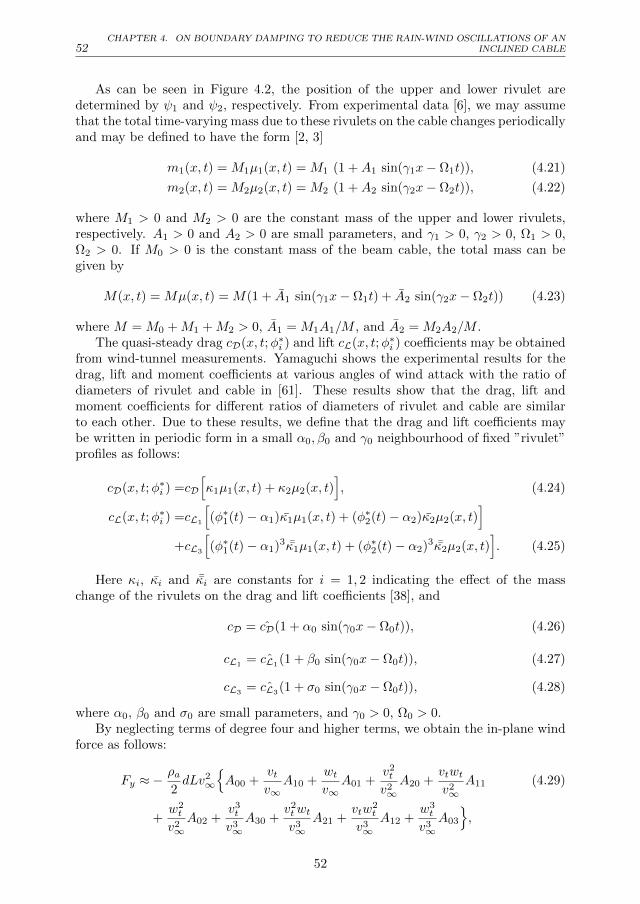
52CHAPTER 4. ON BOUNDARY DAMPING TO REDUCE THE RAIN-WIND OSCILLATIONS OF AN
INCLINED CABLE
As can be seen in Figure 4.2, the position of the upper and lower rivulet aredetermined by ψ1 and ψ2, respectively. From experimental data [6], we may assumethat the total time-varying mass due to these rivulets on the cable changes periodicallyand may be defined to have the form [2, 3]
m1(x, t) = M1µ1(x, t) = M1 (1 +A1 sin(γ1x− Ω1t)), (4.21)
m2(x, t) = M2µ2(x, t) = M2 (1 +A2 sin(γ2x− Ω2t)), (4.22)
where M1 > 0 and M2 > 0 are the constant mass of the upper and lower rivulets,respectively. A1 > 0 and A2 > 0 are small parameters, and γ1 > 0, γ2 > 0, Ω1 > 0,Ω2 > 0. If M0 > 0 is the constant mass of the beam cable, the total mass can begiven by
M(x, t) = Mµ(x, t) = M(1 + A1 sin(γ1x− Ω1t) + A2 sin(γ2x− Ω2t)) (4.23)
where M = M0 +M1 +M2 > 0, A1 = M1A1/M , and A2 = M2A2/M .The quasi-steady drag cD(x, t;φ∗i ) and lift cL(x, t;φ∗i ) coefficients may be obtained
from wind-tunnel measurements. Yamaguchi shows the experimental results for thedrag, lift and moment coefficients at various angles of wind attack with the ratio ofdiameters of rivulet and cable in [61]. These results show that the drag, lift andmoment coefficients for different ratios of diameters of rivulet and cable are similarto each other. Due to these results, we define that the drag and lift coefficients maybe written in periodic form in a small α0, β0 and γ0 neighbourhood of fixed ”rivulet”profiles as follows:
cD(x, t;φ∗i ) =cD
[κ1µ1(x, t) + κ2µ2(x, t)
], (4.24)
cL(x, t;φ∗i ) =cL1
[(φ∗1(t)− α1)κ1µ1(x, t) + (φ∗2(t)− α2)κ2µ2(x, t)
]+cL3
[(φ∗1(t)− α1)3 ¯κ1µ1(x, t) + (φ∗2(t)− α2)3 ¯κ2µ2(x, t)
]. (4.25)
Here κi, κi and ¯κi are constants for i = 1, 2 indicating the effect of the masschange of the rivulets on the drag and lift coefficients [38], and
cD = cD(1 + α0 sin(γ0x− Ω0t)), (4.26)
cL1= ˆcL1
(1 + β0 sin(γ0x− Ω0t)), (4.27)
cL3= ˆcL3
(1 + σ0 sin(γ0x− Ω0t)), (4.28)
where α0, β0 and σ0 are small parameters, and γ0 > 0, Ω0 > 0.By neglecting terms of degree four and higher terms, we obtain the in-plane wind
force as follows:
Fy ≈−ρa2dLv2
∞
A00 +
vtv∞
A10 +wtv∞
A01 +v2t
v2∞A20 +
vtwtv2∞A11 (4.29)
+w2t
v2∞A02 +
v3t
v3∞A30 +
v2twtv3∞
A21 +vtw
2t
v3∞
A12 +w3t
v3∞A03
,
52

4.3. FURTHER SIMPLIFICATIONS 53
and similarly, we compute the out-of-plane wind force as follows:
Fz ≈ρa2dLv2
∞
B00 +
vtv∞
B10 +wtv∞
B01 +v2t
v2∞B20 +
vtwtv2∞B11 (4.30)
+w2t
v2∞B02 +
v3t
v3∞B30 +
v2twtv3∞
B21 +vtw
2t
v3∞
B12 +w3t
v3∞B03
,
where Aij and Bij for i, j = 0, 1, 2, 3 as follows:
Aij =cD
[κ1µ1(x, t) + κ2µ2(x, t)
]aij0 + cL1
[κ1µ1(x, t)aij1 + κ2µ2(x, t)aij2
](4.31)
+cL3
[¯κ1µ1(x, t)aij3 + ¯κ2µ2(x, t)aij4
],
and
Bij =cD
[κ1µ1(x, t) + κ2µ2(x, t)
]bij0 + cL1
[κ1µ1(x, t)bij1 + κ2µ2(x, t)bij2
](4.32)
+cL3
[¯κ1µ1(x, t)bij3 + ¯κ2µ2(x, t)bij4
].
The detailed expressions of the aijk- and bijk-coefficients for k = 1, 2, 3, 4 can befound in Appendix A. When we assume only in-plane horizontal cable motion withonly the upper rivulet present, that is, γ(α, β) = 0, µ2(x, t) = 0, and κ1 = κ1 = ¯κ1 =µ1(x, t) = 1, the same coefficients of cD, cL1
and cL3are obtained as in [56].
4.3 Further Simplifications
For further calculations, we only consider in-plane motion (w = 0) of the inclinedbeam, and we assume that there is only one rivulet on the cable, that is, γ1 ≈ γ2,Ω1 ≈ Ω2. Thus, we define M(x, t) = M(1 + Asin(γ1x − Ω1t)), where A is a smallparameter. We substitute Eq. (4.29) and Eq. (4.30), into Eq. (4.12)-(4.13) and rewritein order to obtain the equations of motion for the beam with a time-varying mass,yielding
utt −E
M
∂
∂x
(ux +
v2x
2
)=[A Ω1 cos(γ1x− Ω1t)
]ut (4.33)
−[Asin(γ1x− Ω1t)
]utt,
+[A γ1 cos(γ1x− Ω1t)
]g sin(α)x
+[2 + 2A sin(γ1x− Ω1t)
]g sin(α),
53

54CHAPTER 4. ON BOUNDARY DAMPING TO REDUCE THE RAIN-WIND OSCILLATIONS OF AN
INCLINED CABLE
EIyAM
vxxxx −T0
AMvxx + vtt−
E
M
∂
∂x
[vx
(ux +
v2x
2
)]=[A Ω1 cos(γ1x− Ω1t)
]vt
(4.34)
−[A sin(γ1x− Ω1t)
]vtt
+[A γ1 cos(γ1x− Ω1t)
]g sin(α)xvx
+[1 + A sin(γ1x− Ω1t)
]g sin(α)xvxx
+[1 + A sin(γ1x− Ω1t)
]g sin(α)vx
+[1 + A sin(γ1x− Ω1t)
]g cos(α)
− ρa2AM
dLv2∞
A00 +
vtv∞
A10 +v2t
v2∞A20 +
v3t
v3∞A30
,
where Aij for i, j = 0, 1, 2, 3 are defined in Eq. (4.31). Eq. (4.33)-(4.34) represent thein-plane motion of the inclined beam cable system in the longitudinal and transversaldirection, that is, in x-, and y-direction. We introduce the new variables u(x, t) andv(x, t) as defined by:
u(x, t) = u(x, t) + u(x), (4.35)
v(x, t) = v(x, t) + v(x), (4.36)
where u(x) and v(x) are the ”stationary” solutions by neglecting small time pertur-bation (see Appendix B.). When we substitute the new variables Eq. (4.35)-(4.36)into the Eq. (4.33)-(4.34), we obtain
utt −E
M
∂
∂x
(ux + vxvx +
v2x
2
)=[A Ω1 cos(γ1x− Ω1t)
]ut (4.37)
−[Asin(γ1x− Ω1t)
]utt
+[A γ1 cos(γ1x− Ω1t)
]g sin(α)x
+[2A sin(γ1x− Ω1t)
]g sin(α),
54

4.3. FURTHER SIMPLIFICATIONS 55
EIyAM
vxxxx −T0
AMvxx+vtt −
E
M
∂
∂x
[(vx + vx)
(ux + vxvx +
v2x
2
)(4.38)
+vx
(ux +
v2x
2
)]=[A Ω1 cos(γ1x− Ω1t)
]vt
−[A sin(γ1x− Ω1t)
]vtt
+[A γ1 cos(γ1x− Ω1t)
]g sin(α)x(vx + vx)
+[A sin(γ1x− Ω1t)
]g sin(α)x(vxx + vxx)
+g sin(α)xvxx + g sin(α)vx
+[A sin(γ1x− Ω1t)
]g sin(α)(vx + vx)
+[A sin(γ1x− Ω1t)
]g cos(α)
− ρa2AM
dLv2∞
vtv∞
A10 +v2t
v2∞A20 +
v3t
v3∞A30
.
These coupled partial differential equations can be reduced to a single partialdifferential equation by applying Kirchhoff’s approximation. It will be assumed thatu and u are O(ε2), v and v are O(ε), A is O(ε), gsin(α) = P ∗0 is O(1), and E
M = P ∗1is O(1/ε), where ε is a small parameter with 0 < ε 1. Then, by using theseassumptions, Eq. (4.37) up to order ε becomes
−P ∗1∂
∂x
(ux + vxvx +
v2x
2
)= P ∗0
[2A sin(γ1x−Ω1t) + A γ1x cos(γ1x−Ω1t)
](4.39)
First we integrate Eq. (4.39) with respect to x from 0 to x, yielding
−P ∗1(ux + vxvx +
v2x
2
)= −h(t) +
∫ x
0
2P ∗0 A sin(γ1x− Ω1t)dx (4.40)
+
∫ x
0
P ∗0 A γ1x cos(γ1x− Ω1t)dx,
and then from 0 to L, obtaining
−P ∗1[u(L, t)− u(0, t)+
∫ L
0
(vxvx +
v2x
2
)dx]
= −∫ L
0
h(t)dx (4.41)
+
∫ L
0
∫ x
0
2P ∗0 A sin(γ1x− Ω1t)dxdx
+
∫ L
0
∫ x
0
P ∗0 A γ1x cos(γ1x− Ω1t)dxdx,
Hence,
h(t) =P ∗1L
[u(L, t)− u(0, t)+
∫ L
0
(vxvx+
v2x
2
)dx]
+AP ∗0γ1
(cos(Ω1t)−cos(γ1L−Ω1t)
).
(4.42)
55
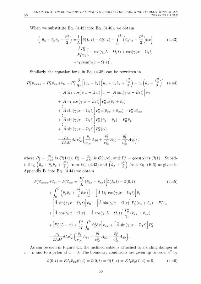
56CHAPTER 4. ON BOUNDARY DAMPING TO REDUCE THE RAIN-WIND OSCILLATIONS OF AN
INCLINED CABLE
When we substitute Eq. (4.42) into Eq. (4.40), we obtain(ux + vxvx +
v2x
2
)=
1
L
[u(L, t)− u(0, t) +
∫ L
0
(vxvx +
v2x
2
)dx]
(4.43)
+AP ∗0P ∗1 γ1
[− cos(γ1L− Ω1t) + cos(γ1x− Ω1t)
−γ1xsin(γ1x− Ω1t)].
Similarly the equation for v in Eq. (4.38) can be rewritten in
P ∗2 vxxxx − P ∗3 vxx+vtt − P ∗1∂
∂x
[(vx + vx)
(ux + vxvx +
v2x
2
)+ vx
(ux +
v2x
2
)](4.44)
=[A Ω1 cos(γ1x− Ω1t)
]vt −
[A sin(γ1x− Ω1t)
]vtt
+[A γ1 cos(γ1x− Ω1t)
]P ∗0 x(vx + vx)
+[A sin(γ1x− Ω1t)
]P ∗0 x(vxx + vxx) + P ∗0 xvxx
+[A sin(γ1x− Ω1t)
]P ∗0 (vx + vx) + P ∗0 vx
+[A sin(γ1x− Ω1t)
]P ∗4 (α)
− ρa2AM
dLv2∞
vtv∞
A10 +v2t
v2∞A20 +
v3t
v3∞A30
,
where P ∗2 =EIyAM is O(1/ε), P ∗3 = T0
AM is O(1/ε), and P ∗4 = gcos(α) is O(1) . Substi-
tuting(ux + vxvx +
v2x2
)from Eq. (4.43) and
(ux +
v2x2
)from Eq. (B.6) as given in
Appendix B. into Eq. (4.44) we obtain
P ∗2 vxxxx+vtt − P ∗3 vxx =P ∗1L
(vxx + vxx)[u(L, t)− u(0, t) (4.45)
+
∫ L
0
(vxvx +
v2x
2dx)]
+[A Ω1 cos(γ1x− Ω1t)
]vt
−[A sin(γ1x− Ω1t)
]vtt −
[A sin(γ1x− Ω1t)
]P ∗0 (vx + vx)− P ∗0 vx
+[A cos(γ1x− Ω1t)− A cos(γ1L− Ω1t)
]P ∗0γ1
(vxx + vxx)
+[P ∗0 (L− x) +
P ∗12L
∫ L
0
v2xdx
]vxx +
[A sin(γ1x− Ω1t)
]P ∗4
− ρa2AM
dLv2∞
vtv∞
A10 +v2t
v2∞A20 +
v3t
v3∞A30
.
As can be seen in Figure 4.1, the inclined cable is attached to a sliding damper atx = L and to a pylon at x = 0. The boundary conditions are given up to order ε2 by
u(0, t) = EIy vxx(0, t) = v(0, t) = u(L, t) = EIy vx(L, t) = 0, (4.46)
56
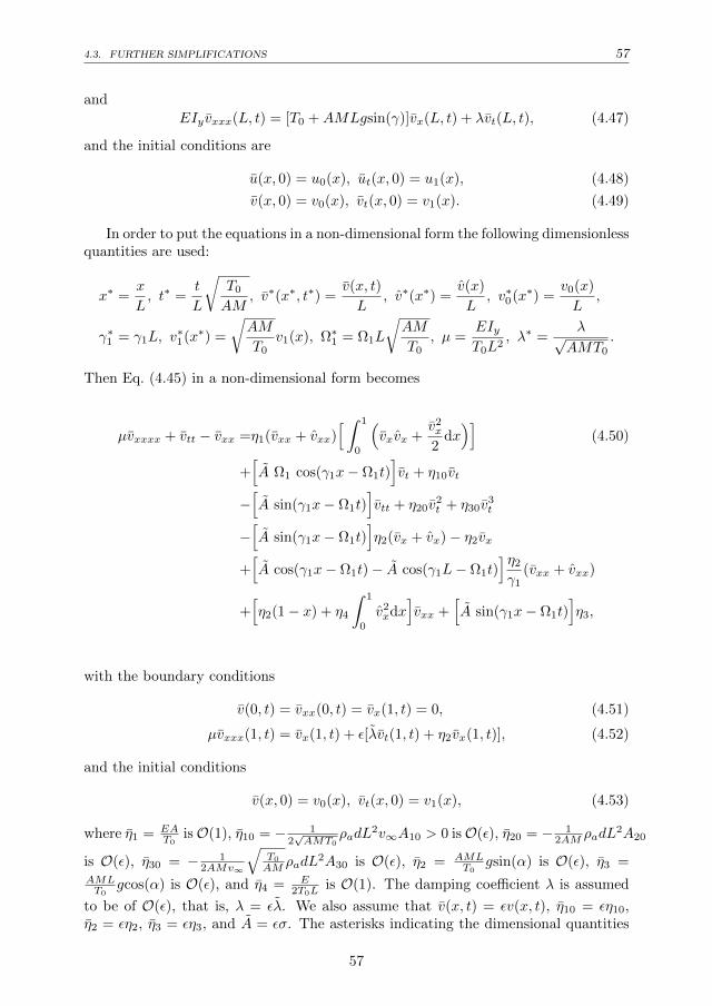
4.3. FURTHER SIMPLIFICATIONS 57
and
EIy vxxx(L, t) = [T0 +AMLgsin(γ)]vx(L, t) + λvt(L, t), (4.47)
and the initial conditions are
u(x, 0) = u0(x), ut(x, 0) = u1(x), (4.48)
v(x, 0) = v0(x), vt(x, 0) = v1(x). (4.49)
In order to put the equations in a non-dimensional form the following dimensionlessquantities are used:
x∗ =x
L, t∗ =
t
L
√T0
AM, v∗(x∗, t∗) =
v(x, t)
L, v∗(x∗) =
v(x)
L, v∗0(x∗) =
v0(x)
L,
γ∗1 = γ1L, v∗1(x∗) =
√AM
T0v1(x), Ω∗1 = Ω1L
√AM
T0, µ =
EIyT0L2
, λ∗ =λ√
AMT0
.
Then Eq. (4.45) in a non-dimensional form becomes
µvxxxx + vtt − vxx =η1(vxx + vxx)[ ∫ 1
0
(vxvx +
v2x
2dx)]
(4.50)
+[A Ω1 cos(γ1x− Ω1t)
]vt + η10vt
−[A sin(γ1x− Ω1t)
]vtt + η20v
2t + η30v
3t
−[A sin(γ1x− Ω1t)
]η2(vx + vx)− η2vx
+[A cos(γ1x− Ω1t)− A cos(γ1L− Ω1t)
]η2
γ1(vxx + vxx)
+[η2(1− x) + η4
∫ 1
0
v2xdx
]vxx +
[A sin(γ1x− Ω1t)
]η3,
with the boundary conditions
v(0, t) = vxx(0, t) = vx(1, t) = 0, (4.51)
µvxxx(1, t) = vx(1, t) + ε[λvt(1, t) + η2vx(1, t)], (4.52)
and the initial conditions
v(x, 0) = v0(x), vt(x, 0) = v1(x), (4.53)
where η1 = EAT0
isO(1), η10 = − 12√AMT0
ρadL2v∞A10 > 0 isO(ε), η20 = − 1
2AM ρadL2A20
is O(ε), η30 = − 12AMv∞
√T0
AM ρadL2A30 is O(ε), η2 = AML
T0gsin(α) is O(ε), η3 =
AMLT0
gcos(α) is O(ε), and η4 = E2T0L
is O(1). The damping coefficient λ is assumed
to be of O(ε), that is, λ = ελ. We also assume that v(x, t) = εv(x, t), η10 = εη10,η2 = εη2, η3 = εη3, and A = εσ. The asterisks indicating the dimensional quantities
57
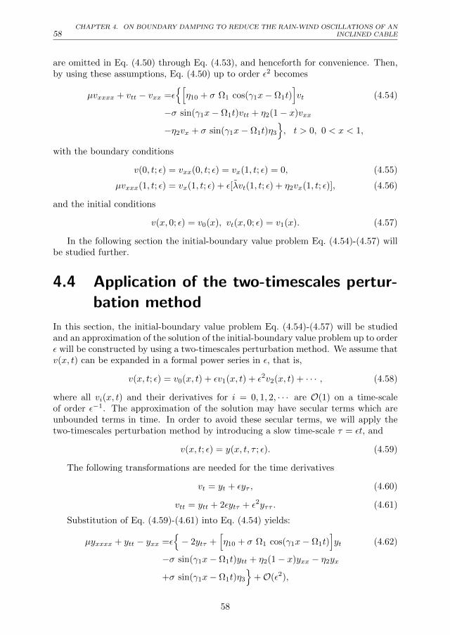
58CHAPTER 4. ON BOUNDARY DAMPING TO REDUCE THE RAIN-WIND OSCILLATIONS OF AN
INCLINED CABLE
are omitted in Eq. (4.50) through Eq. (4.53), and henceforth for convenience. Then,by using these assumptions, Eq. (4.50) up to order ε2 becomes
µvxxxx + vtt − vxx =ε[η10 + σ Ω1 cos(γ1x− Ω1t)
]vt (4.54)
−σ sin(γ1x− Ω1t)vtt + η2(1− x)vxx
−η2vx + σ sin(γ1x− Ω1t)η3
, t > 0, 0 < x < 1,
with the boundary conditions
v(0, t; ε) = vxx(0, t; ε) = vx(1, t; ε) = 0, (4.55)
µvxxx(1, t; ε) = vx(1, t; ε) + ε[λvt(1, t; ε) + η2vx(1, t; ε)], (4.56)
and the initial conditions
v(x, 0; ε) = v0(x), vt(x, 0; ε) = v1(x). (4.57)
In the following section the initial-boundary value problem Eq. (4.54)-(4.57) willbe studied further.
4.4 Application of the two-timescales pertur-bation method
In this section, the initial-boundary value problem Eq. (4.54)-(4.57) will be studiedand an approximation of the solution of the initial-boundary value problem up to orderε will be constructed by using a two-timescales perturbation method. We assume thatv(x, t) can be expanded in a formal power series in ε, that is,
v(x, t; ε) = v0(x, t) + εv1(x, t) + ε2v2(x, t) + · · · , (4.58)
where all vi(x, t) and their derivatives for i = 0, 1, 2, · · · are O(1) on a time-scaleof order ε−1. The approximation of the solution may have secular terms which areunbounded terms in time. In order to avoid these secular terms, we will apply thetwo-timescales perturbation method by introducing a slow time-scale τ = εt, and
v(x, t; ε) = y(x, t, τ ; ε). (4.59)
The following transformations are needed for the time derivatives
vt = yt + εyτ , (4.60)
vtt = ytt + 2εytτ + ε2yττ . (4.61)
Substitution of Eq. (4.59)-(4.61) into Eq. (4.54) yields:
µyxxxx + ytt − yxx =ε− 2ytτ +
[η10 + σ Ω1 cos(γ1x− Ω1t)
]yt (4.62)
−σ sin(γ1x− Ω1t)ytt + η2(1− x)yxx − η2yx
+σ sin(γ1x− Ω1t)η3
+O(ε2),
58
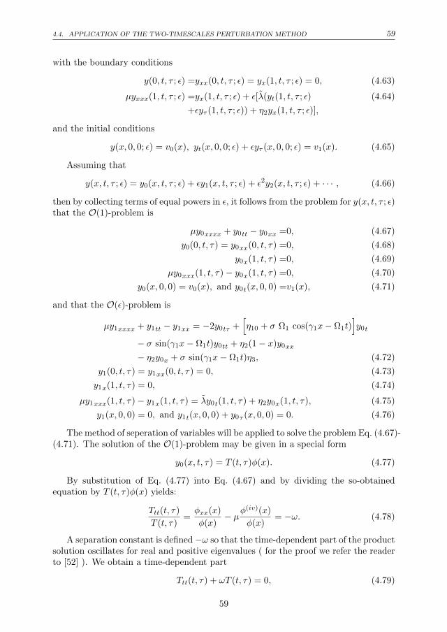
4.4. APPLICATION OF THE TWO-TIMESCALES PERTURBATION METHOD 59
with the boundary conditions
y(0, t, τ ; ε) =yxx(0, t, τ ; ε) = yx(1, t, τ ; ε) = 0, (4.63)
µyxxx(1, t, τ ; ε) =yx(1, t, τ ; ε) + ε[λ(yt(1, t, τ ; ε) (4.64)
+εyτ (1, t, τ ; ε)) + η2yx(1, t, τ ; ε)],
and the initial conditions
y(x, 0, 0; ε) = v0(x), yt(x, 0, 0; ε) + εyτ (x, 0, 0; ε) = v1(x). (4.65)
Assuming that
y(x, t, τ ; ε) = y0(x, t, τ ; ε) + εy1(x, t, τ ; ε) + ε2y2(x, t, τ ; ε) + · · · , (4.66)
then by collecting terms of equal powers in ε, it follows from the problem for y(x, t, τ ; ε)that the O(1)-problem is
µy0xxxx + y0tt − y0xx =0, (4.67)
y0(0, t, τ) = y0xx(0, t, τ) =0, (4.68)
y0x(1, t, τ) =0, (4.69)
µy0xxx(1, t, τ)− y0x(1, t, τ) =0, (4.70)
y0(x, 0, 0) = v0(x), and y0t(x, 0, 0) =v1(x), (4.71)
and that the O(ε)-problem is
µy1xxxx + y1tt − y1xx = −2y0tτ +[η10 + σ Ω1 cos(γ1x− Ω1t)
]y0t
− σ sin(γ1x− Ω1t)y0tt + η2(1− x)y0xx
− η2y0x + σ sin(γ1x− Ω1t)η3, (4.72)
y1(0, t, τ) = y1xx(0, t, τ) = 0, (4.73)
y1x(1, t, τ) = 0, (4.74)
µy1xxx(1, t, τ)− y1x(1, t, τ) = λy0t(1, t, τ) + η2y0x(1, t, τ), (4.75)
y1(x, 0, 0) = 0, and y1t(x, 0, 0) + y0τ (x, 0, 0) = 0. (4.76)
The method of seperation of variables will be applied to solve the problem Eq. (4.67)-(4.71). The solution of the O(1)-problem may be given in a special form
y0(x, t, τ) = T (t, τ)φ(x). (4.77)
By substitution of Eq. (4.77) into Eq. (4.67) and by dividing the so-obtainedequation by T (t, τ)φ(x) yields:
Ttt(t, τ)
T (t, τ)=φxx(x)
φ(x)− µφ
(iv)(x)
φ(x)= −ω. (4.78)
A separation constant is defined−ω so that the time-dependent part of the productsolution oscillates for real and positive eigenvalues ( for the proof we refer the readerto [52] ). We obtain a time-dependent part
Ttt(t, τ) + ωT (t, τ) = 0, (4.79)
59
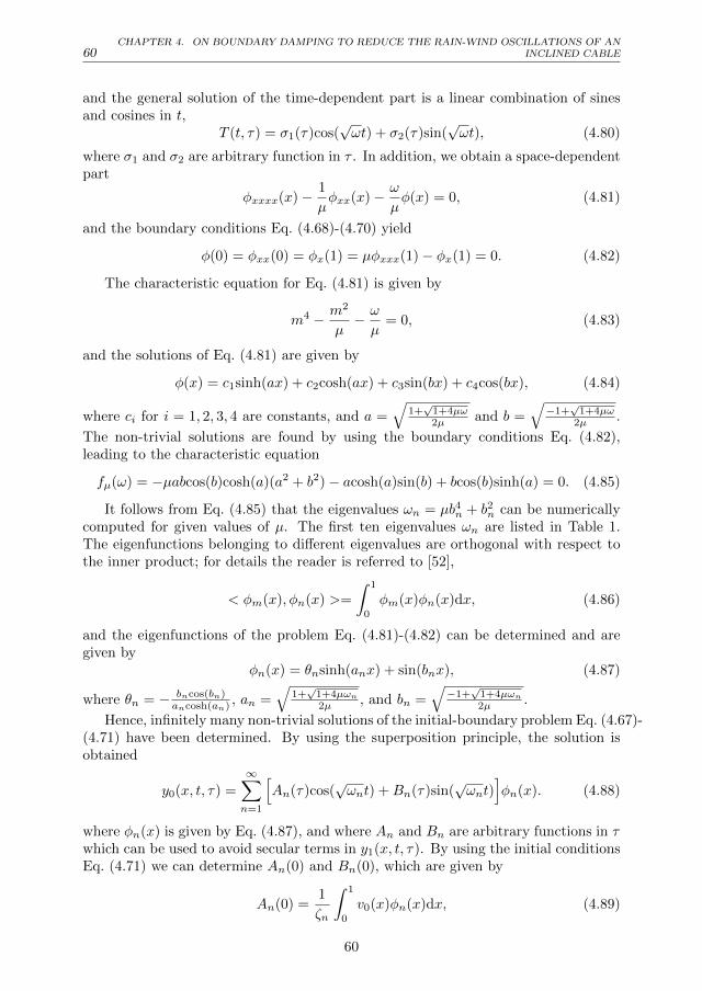
60CHAPTER 4. ON BOUNDARY DAMPING TO REDUCE THE RAIN-WIND OSCILLATIONS OF AN
INCLINED CABLE
and the general solution of the time-dependent part is a linear combination of sinesand cosines in t,
T (t, τ) = σ1(τ)cos(√ωt) + σ2(τ)sin(
√ωt), (4.80)
where σ1 and σ2 are arbitrary function in τ . In addition, we obtain a space-dependentpart
φxxxx(x)− 1
µφxx(x)− ω
µφ(x) = 0, (4.81)
and the boundary conditions Eq. (4.68)-(4.70) yield
φ(0) = φxx(0) = φx(1) = µφxxx(1)− φx(1) = 0. (4.82)
The characteristic equation for Eq. (4.81) is given by
m4 − m2
µ− ω
µ= 0, (4.83)
and the solutions of Eq. (4.81) are given by
φ(x) = c1sinh(ax) + c2cosh(ax) + c3sin(bx) + c4cos(bx), (4.84)
where ci for i = 1, 2, 3, 4 are constants, and a =√
1+√
1+4µω2µ and b =
√−1+
√1+4µω
2µ .
The non-trivial solutions are found by using the boundary conditions Eq. (4.82),leading to the characteristic equation
fµ(ω) = −µabcos(b)cosh(a)(a2 + b2)− acosh(a)sin(b) + bcos(b)sinh(a) = 0. (4.85)
It follows from Eq. (4.85) that the eigenvalues ωn = µb4n + b2n can be numericallycomputed for given values of µ. The first ten eigenvalues ωn are listed in Table 1.The eigenfunctions belonging to different eigenvalues are orthogonal with respect tothe inner product; for details the reader is referred to [52],
< φm(x), φn(x) >=
∫ 1
0
φm(x)φn(x)dx, (4.86)
and the eigenfunctions of the problem Eq. (4.81)-(4.82) can be determined and aregiven by
φn(x) = θnsinh(anx) + sin(bnx), (4.87)
where θn = − bncos(bn)ancosh(an) , an =
√1+√
1+4µωn2µ , and bn =
√−1+
√1+4µωn2µ .
Hence, infinitely many non-trivial solutions of the initial-boundary problem Eq. (4.67)-(4.71) have been determined. By using the superposition principle, the solution isobtained
y0(x, t, τ) =
∞∑n=1
[An(τ)cos(
√ωnt) +Bn(τ)sin(
√ωnt)
]φn(x). (4.88)
where φn(x) is given by Eq. (4.87), and where An and Bn are arbitrary functions in τwhich can be used to avoid secular terms in y1(x, t, τ). By using the initial conditionsEq. (4.71) we can determine An(0) and Bn(0), which are given by
An(0) =1
ζn
∫ 1
0
v0(x)φn(x)dx, (4.89)
60

4.4. APPLICATION OF THE TWO-TIMESCALES PERTURBATION METHOD 61
and√ωnBn(0) =
1
ζn
∫ 1
0
v1(x)φn(x)dx, (4.90)
where
ζn =
∫ 1
0
φ2n(x)dx. (4.91)
Table 4.1: Some eigenvalues ωi which are roots of Eq. (4.85) with ωi the i-th root.
ω µ = 0.001 µ = 0.01 µ = 0.1 µ = 1
ω1 4.16497 4.30777 5.00501 10.54607
ω2 24.68972 29.20039 73.56205 517.34633
ω3 67.51921 101.78930 444.20353 3868.72929
ω4 137.55593 269.11062 1584.65381 14740.35501
ω5 241.83773 601.31819 4196.24404 40145.67525
ω6 389.72154 1191.92269 9214.09788 89435.96197
ω7 592.89840 2157.81266 17807.12342 174300.30645
ω8 865.39593 3639.25581 31378.01114 308765.61727
ω9 1223.57912 5799.89869 51563.23375 509196.62255
ω10 1686.15056 8826.76635 80233.04556 794295.86667
Now we solve the O(ε)-problem Eq. (4.72)-(4.76). Due to having an inhomoge-neous boundary condition Eq. (4.75), we use the following transformation to convertthe problem into a problem with homogeneous boundary conditions
y1(x, t, τ) = V (x, t, τ) +(x4 − 2x3
12µ+ 2
)h(t, τ), (4.92)
whereh(t, τ) = λy0t(1, t, τ) + η2y0x(1, t, τ). (4.93)
Substituting Eq. (4.92) into Eq. (4.72)-(4.76), we obtain
µVxxxx + Vtt − Vxx = −2y0tτ +[η10 + σ Ω1 cos(γ1x− Ω1t)
]y0t − η2y0x (4.94)
− σ sin(γ1x− Ω1t)y0tt + η2(1− x)y0xx + σ sin(γ1x− Ω1t)η3
+(12x2 − 12x− 24µ
12µ+ 2
)h(t, τ)−
(x4 − 2x3
12µ+ 2
)htt(t, τ),
V (0, t, τ) = Vxx(0, t, τ) = Vx(1, t, τ)−( 2
12µ+ 2
)h(t, τ) = 0, (4.95)
µVxxx(1, t, τ)− Vx(1, t, τ) = 0, (4.96)
61
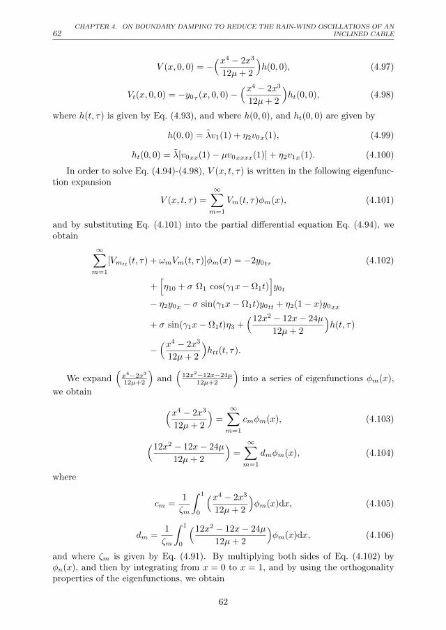
62CHAPTER 4. ON BOUNDARY DAMPING TO REDUCE THE RAIN-WIND OSCILLATIONS OF AN
INCLINED CABLE
V (x, 0, 0) = −(x4 − 2x3
12µ+ 2
)h(0, 0), (4.97)
Vt(x, 0, 0) = −y0τ (x, 0, 0)−(x4 − 2x3
12µ+ 2
)ht(0, 0), (4.98)
where h(t, τ) is given by Eq. (4.93), and where h(0, 0), and ht(0, 0) are given by
h(0, 0) = λv1(1) + η2v0x(1), (4.99)
ht(0, 0) = λ[v0xx(1)− µv0xxxx(1)] + η2v1x(1). (4.100)
In order to solve Eq. (4.94)-(4.98), V (x, t, τ) is written in the following eigenfunc-tion expansion
V (x, t, τ) =
∞∑m=1
Vm(t, τ)φm(x), (4.101)
and by substituting Eq. (4.101) into the partial differential equation Eq. (4.94), weobtain
∞∑m=1
[Vmtt(t, τ) + ωmVm(t, τ)]φm(x) = −2y0tτ (4.102)
+[η10 + σ Ω1 cos(γ1x− Ω1t)
]y0t
− η2y0x − σ sin(γ1x− Ω1t)y0tt + η2(1− x)y0xx
+ σ sin(γ1x− Ω1t)η3 +(12x2 − 12x− 24µ
12µ+ 2
)h(t, τ)
−(x4 − 2x3
12µ+ 2
)htt(t, τ).
We expand(x4−2x3
12µ+2
)and
(12x2−12x−24µ
12µ+2
)into a series of eigenfunctions φm(x),
we obtain (x4 − 2x3
12µ+ 2
)=
∞∑m=1
cmφm(x), (4.103)
(12x2 − 12x− 24µ
12µ+ 2
)=
∞∑m=1
dmφm(x), (4.104)
where
cm =1
ζm
∫ 1
0
(x4 − 2x3
12µ+ 2
)φm(x)dx, (4.105)
dm =1
ζm
∫ 1
0
(12x2 − 12x− 24µ
12µ+ 2
)φm(x)dx, (4.106)
and where ζm is given by Eq. (4.91). By multiplying both sides of Eq. (4.102) byφn(x), and then by integrating from x = 0 to x = 1, and by using the orthogonalityproperties of the eigenfunctions, we obtain
62

4.4. APPLICATION OF THE TWO-TIMESCALES PERTURBATION METHOD 63
[Vntt(t, τ) + ωnVn(t, τ)
]= −cnhtt(t, τ) + dnh(t, τ)− 2Tntτ (t, τ) (4.107)
+η2
ζnTn(t, τ)(Φnn − Φnn)
+η2
ζn
∞∑m=1m 6=n
Tm(t, τ)(Φmn − Φmn)
+σ η3
ζn
(cos(Ω1t)Υn − sin(Ω1t)Υn
)+ η10Tnt(t, τ)
+σ Ω1
ζnTnt(t, τ)
(cos(Ω1t)Ψnn + sin(Ω1t)Ψnn
)+
σ
ζnTntt(t, τ)
(sin(Ω1t)Ψnn − cos(Ω1t)Ψnn
)+
σ
ζn
∞∑m=1m 6=n
[Ω1Tmt(t, τ)
(cos(Ω1t)Ψmn + sin(Ω1t)Ψmn
)+ Tmtt(t, τ)
(sin(Ω1t)Ψmn − cos(Ω1t)Ψmn
)],
where
Tm(t, τ) = Am(τ)cos(√ωmt) +Bm(τ)sin(
√ωmt), (4.108)
and
Φmn =
∫ 1
0
dφm(x)
dxφn(x)dx, (4.109)
Φmn =
∫ 1
0
(1− x)d2φm(x)
dx2φn(x)dx, (4.110)
Ψmn =
∫ 1
0
cos(γ1x)φm(x)φn(x)dx, (4.111)
Ψmn =
∫ 1
0
sin(γ1x)φm(x)φn(x)dx, (4.112)
Υm =
∫ 1
0
cos(γ1x)φm(x)dx, (4.113)
Υm =
∫ 1
0
sin(γ1x)φm(x)dx. (4.114)
It follows from Eq. (4.93) and Eq. (4.88) that h(t, τ) and htt(t, τ) can be writtenas
h(t, τ) = λ
∞∑m=1
Tmt(t, τ)φm(1) + η2
∞∑m=1
Tm(t, τ)dφm(1)
dx, (4.115)
htt(t, τ) = λ
∞∑m=1
Tmttt(t, τ)φm(1) + η2
∞∑m=1
Tmtt(t, τ)dφm(1)
dx. (4.116)
63

64CHAPTER 4. ON BOUNDARY DAMPING TO REDUCE THE RAIN-WIND OSCILLATIONS OF AN
INCLINED CABLE
Hence, by using Eq. (4.115) and Eq. (4.116) it follows that Eq. (4.107) can berewritten as
[Vntt(t, τ) + ωnVn(t, τ)
]= (4.117)
cn
∞∑m=1m6=n
sin(√ωmt)
[− λφm(1)Am(τ)
√ω3m + η2
dφm(1)
dxBm(τ)ωm
]
+ cos(√ωmt)
[λφm(1)Bm(τ)
√ω3m + η2
dφm(1)
dxAm(τ)ωm
]+ dn
∞∑m=1m 6=n
sin(√ωmt)
[− λφm(1)Am(τ)
√ωm + η2
dφm(1)
dxBm(τ)
]
+ cos(√ωmt)
[λφm(1)Bm(τ)
√ωm + η2
dφm(1)
dxAm(τ)
]+η2
ζn
∞∑m=1m6=n
(Φmn − Φmn)[Am(τ)cos(
√ωmt) +Bm(τ)sin(
√ωmt)
]
+ sin(√ωnt)
2√ωn
dAn(τ)
dτ−An(τ)
[η10√ωn + λφn(1)
√ωn(cnωn + dn)
]+Bn(τ)
[η2
ζn(Φnn − Φnn) + η2
dφn(1)
dx(cnωn + dn)
]+ cos(
√ωnt)
− 2√ωn
dBn(τ)
dτ+Bn(τ)
[η10√ωn + λφn(1)
√ωn(cnωn + dn)
]+An(τ)
[η2
ζn(Φnn − Φnn) + η2
dφn(1)
dx(cnωn + dn)
]+σ η3
ζn
(cos(Ω1t)Υn − sin(Ω1t)Υn
)+ sin(Ω1t+
√ωnt)
σ
2ζn(Ω1√ωn + ωn)
[−An(τ)Ψnn +Bn(τ)Ψnn
]+ sin(Ω1t−
√ωnt)
σ
2ζn(Ω1√ωn − ωn)
[An(τ)Ψnn +Bn(τ)Ψnn
]+ cos(Ω1t+
√ωnt)
σ
2ζn(Ω1√ωn + ωn)
[An(τ)Ψnn +Bn(τ)Ψnn
]+ cos(Ω1t−
√ωnt)
σ
2ζn(Ω1√ωn − ωn)
[−An(τ)Ψnn +Bn(τ)Ψnn
]+
σ
2ζn
∞∑m=1m 6=n
sin(Ω1t+
√ωmt)(Ω1
√ωm + ωm)
[−Am(τ)Ψmn +Bm(τ)Ψmn
]+ sin(Ω1t−
√ωmt)(Ω1
√ωm − ωm)
[Am(τ)Ψmn +Bm(τ)Ψmn
]+ cos(Ω1t+
√ωmt)(Ω1
√ωm + ωm)
[Am(τ)Ψmn +Bm(τ)Ψmn
]+ cos(Ω1t−
√ωmt)(Ω1
√ωm − ωm)
[−Am(τ)Ψmn +Bm(τ)Ψmn
].
64

4.4. APPLICATION OF THE TWO-TIMESCALES PERTURBATION METHOD 65
It can be easily seen from Eq. (4.117) that there are infinitely many values of Ω1,which can cause internal resonances. The possible resonance cases are as follow:
(i) The non-resonant case: if Ω1 is not within an order ε-neighbourhood of thefrequencies
√ωn ±
√ωm for all m and n.
(ii) The near resonance case (Resonance detuning): if Ω1 is within an order ε-neighbourhood of
√ωn ±
√ωm for certain fixed m and n.
(iii) The pure resonance case: if Ω1 =√ωn+
√ωm for certain fixed m and n. This
is the sum type resonance case. If Ω1 =√ωn −
√ωm for certain fixed m and n, it is
the difference type resonance case.In the following subsections, we will study the non-resonant case, the sum type
resonance case, the difference type resonance case and by considering only some ofthe first few modes and omitting the higher order modes.
For simplicity we will now assume that Ω1 =√ω1 +
√ω2 (or Ω1 =
√ω2 −
√ω1).
Resonance can occur when Ω1 = ±√ωn ±√ωm for some n and m. We have to
consider the following three cases:(i) Ω1 = −√ωn−
√ωm, which has no solution since the right-hand side is negative
while the left-hand side is positive.(ii) Ω1 =
√ωn +
√ωm, which has only the trivial solution m = 2, n = 1 or m = 1,
n = 2.(iii) Ω1 =
√ωn−
√ωm (or equivalently Ω1 =
√ωm−
√ωn), which has only solutions
by looking at the Table 4.1 for certain values of µ. There are possibilities that threemodes are interacting. For example,
√ω1 +
√ω2∼=√ω4 −
√ω2 for µ = 0.001.
Table 4.2: Numerical approximations of ωn and pn = 12φn(1)(cnωn + dn) for
different values of µ.
nµ = 0.001 µ = 0.01 µ = 0.1 µ = 1
ωn pn ωn pn ωn pn ωn pn
1 4.16497 -0.68935 4.30777 -0.74453 5.00501 -0.98509 10.54607 -1.31501
2 24.68972 -0.97241 29.20039 -1.20184 73.56205 -2.39752 517.34633 -4.17474
3 67.51921 -1.05857 101.78930 -1.59718 444.20353 -4.85921 3868.72929 -9.81249
4 137.55593 -1.12954 269.11062 -2.15236 1584.65381 -8.55772 14740.35501 -18.27181
5 241.83773 -1.21100 601.31819 -2.89309 4196.24404 -13.49164 40145.67525 -29.55129
6 389.72154 -1.30902 1191.92269 -3.82147 9214.09788 -19.65981 89435.96197 -43.65071
7 592.89840 -1.42560 2157.81266 -4.93712 17807.12342 -27.06189 174300.30645 -60.57004
8 865.39593 -1.56152 3639.25581 -6.23961 31378.01114 -35.69774 308765.61727 -80.30926
9 1223.57912 -1.71708 5799.89869 -7.72870 51563.23375 -45.56732 509196.62255 -102.86836
10 1686.15056 -1.89241 8826.76635 -9.40424 80233.04556 -56.67063 794295.86667 -128.24735
25 41022.73344 -6.88972 356891.24613 -56.88899 3515576.38882 -371.26434 35102427.80053 -847.31857
50 609002.39910 -25.03887 5872359.00977 -229.14149 58505925.11380 -1512.43738 584841586.15436 -3455.71402
65
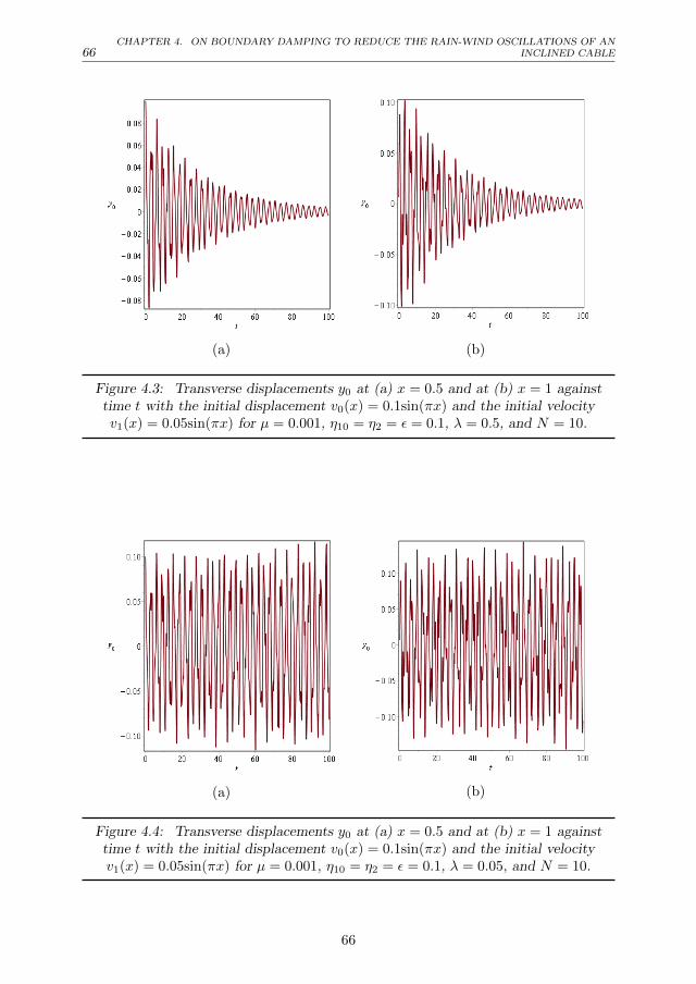
66CHAPTER 4. ON BOUNDARY DAMPING TO REDUCE THE RAIN-WIND OSCILLATIONS OF AN
INCLINED CABLE
(a) (b)
Figure 4.3: Transverse displacements y0 at (a) x = 0.5 and at (b) x = 1 againsttime t with the initial displacement v0(x) = 0.1sin(πx) and the initial velocityv1(x) = 0.05sin(πx) for µ = 0.001, η10 = η2 = ε = 0.1, λ = 0.5, and N = 10.
(a) (b)
Figure 4.4: Transverse displacements y0 at (a) x = 0.5 and at (b) x = 1 againsttime t with the initial displacement v0(x) = 0.1sin(πx) and the initial velocityv1(x) = 0.05sin(πx) for µ = 0.001, η10 = η2 = ε = 0.1, λ = 0.05, and N = 10.
66
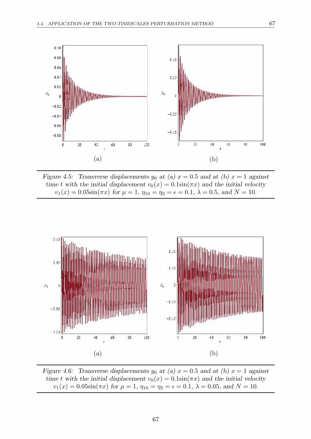
4.4. APPLICATION OF THE TWO-TIMESCALES PERTURBATION METHOD 67
(a) (b)
Figure 4.5: Transverse displacements y0 at (a) x = 0.5 and at (b) x = 1 againsttime t with the initial displacement v0(x) = 0.1sin(πx) and the initial velocity
v1(x) = 0.05sin(πx) for µ = 1, η10 = η2 = ε = 0.1, λ = 0.5, and N = 10.
(a) (b)
Figure 4.6: Transverse displacements y0 at (a) x = 0.5 and at (b) x = 1 againsttime t with the initial displacement v0(x) = 0.1sin(πx) and the initial velocityv1(x) = 0.05sin(πx) for µ = 1, η10 = η2 = ε = 0.1, λ = 0.05, and N = 10.
67

68CHAPTER 4. ON BOUNDARY DAMPING TO REDUCE THE RAIN-WIND OSCILLATIONS OF AN
INCLINED CABLE
4.4.1 The non-resonant case
When Ω1 6=√ωn ±
√ωm + O(ε) for all m and n only resonances occur due to the
fourth and fifth term in the right hand side of Eq. (4.117), that is, Eq. (4.117) can berewritten as
[Vntt(t, τ)+ωnVn(t, τ)
]= sin(
√ωnt)
2√ωn
dAn(τ)
dτ(4.118)
−An(τ)[η10√ωn + λφn(1)
√ωn(cnωn + dn)
]+Bn(τ)
[η2
ζn(Φnn − Φnn) + η2
dφn(1)
dx(cnωn + dn)
]+ cos(
√ωnt)
− 2√ωn
dBn(τ)
dτ
+Bn(τ)[η10√ωn + λφn(1)
√ωn(cnωn + dn)
]+An(τ)
[η2
ζn(Φnn − Φnn) + η2
dφn(1)
dx(cnωn + dn)
]+ “NST”,
where “NST” stands for terms that lead to nonsecular terms in Vn. In order to removesecular terms, it follows from Eq. (4.118) that An(τ) and Bn(τ) have to satisfy
dAn(τ)
dτ−An(τ)Xn +Bn(τ)Yn = 0, (4.119)
dBn(τ)
dτ−Bn(τ)Xn −An(τ)Yn = 0, (4.120)
where Xn and Yn are defined by
Xn =[η10
2+λ
2φn(1)(cnωn + dn)
], (4.121)
Yn =[ η2
2ζn√ωn
(Φnn − Φnn) +η2
2√ωn
dφn(1)
dx(cnωn + dn)
]. (4.122)
The solution of Eq. (4.119) and Eq. (4.120) is given by
An(τ) =[An(0)cos(Ynτ)−Bn(0)sin(Ynτ)
]eXnτ , (4.123)
Bn(τ) =[An(0)sin(Ynτ) +Bn(0)cos(Ynτ)
]eXnτ , (4.124)
where An(0) and Bn(0) are given by Eq. (4.89) and Eq. (4.90), respectively. By usingEq. (4.105) and Eq. (4.106) with Eq. (4.81) and Eq. (4.82) it can easily be shown that12 (cnωn + dn) = µ
ζn(12µ+2)d2φn(1)
dx2 − 12ζn
φn(1). Hence Eq. (4.108) with Eq. (4.123) and
Eq. (4.124) can be rewritten as
Tm(t, τ) = eXmτ[Am(0)cos(
√ωmt− Ymτ) +Bm(0)sin(
√ωmt− Ymτ)
]. (4.125)
68

4.4. APPLICATION OF THE TWO-TIMESCALES PERTURBATION METHOD 69
Now, from Eq. (4.118) with Eq. (4.119)-(4.125), we can obtain Vn(t, τ) straight-forwardly. Obviously, Vn(t, τ) will be bounded on a time-scale of order 1/ε, and sowill be Vn(x, t, τ).
In Table 4.2 numerical approximations of ωn and the damping parameter pn aregiven for different values of µ. For different bending stiffness, we can choose the damp-ing parameter in such a way that all modes are damped by taking λ appropriatelycompared to the η10 coefficient. It is also clear to see from Table 4.2 that for smallervalues of µ we should take larger λ to have damping for all modes. In Table 4.3, itcan be seen as expected that the bending stiffness µ and the damping parameter λinfluence the stability.
For µ = 0.001, Figure. 4.3 and Figure. 4.4 demonstrate the vibration response atthe middle x = 0.5 and at the end x = 1 points of the beam for different values of thedamping factor λ, Figure. 4.3 is plotted for λ = 0.5 and Figures. 4.4 is plotted for λ =2; the initial conditions are specified as v0(x) = 0.1sin(πx) and v1(x) = 0.05sin(πx).For µ = 1, Figure. 4.5 and Figure. 4.6 illustrate similar behaviour. These figuresshow that the amplitudes of the transverse vibrations decrease faster for increasingof µ and λ. Similar results for the string-like problem have been observed in [20].
4.4.2 The sum type resonance case: Ω1 =√ω2 +
√ω1
We will consider now only the first two modes and omit the higher order modes. Thatis, we will assume that for the given µ values only these two modes might occur in aresonance interaction. Eq. (4.117) can be rewritten as
[V1tt(t, τ)+ω1V1(t, τ)
]= sin(
√ω1t)
2√ω1
dA1(τ)
dτ(4.126)
−A1(τ)[η10√ω1 + λφ1(1)
√ω1(c1ω1 + d1)
]+B1(τ)
[η2
ζ1(Φ11 − Φ11) + η2
dφ1(1)
dx(c1ω1 + d1)
]+ cos(
√ω1t)
− 2√ω1
dB1(τ)
dτ
+B1(τ)[η10√ω1 + λφ1(1)
√ω1(c1ω1 + d1)
]+A1(τ)
[η2
ζ1(Φ11 − Φ11) + η2
dφ1(1)
dx(c1ω1 + d1)
]+ sin(Ω1t−
√ω2t)
σ
2ζ1(Ω1√ω2 − ω2)
[A2(τ)Ψ21 +B2(τ)Ψ21
]+ cos(Ω1t−
√ω2t)
σ
2ζ1(Ω1√ω2 − ω2)
[−A2(τ)Ψ21 +B2(τ)Ψ21
]+ “NST”,
and a similar equation for V2(t, τ) can be obtained from Eq. (4.126). In order to avoidsecular terms, it follows from the equations for V1(t, τ) and V2(t, τ) that A1(τ), B1(τ),A2(τ) and B2(τ) have to satisfy
69

70CHAPTER 4. ON BOUNDARY DAMPING TO REDUCE THE RAIN-WIND OSCILLATIONS OF AN
INCLINED CABLE
dA1(τ)
dτ= A1(τ)X1 −B1(τ)Y1 −A2(τ)Z2 −B2(τ)C2, (4.127)
dB1(τ)
dτ= A1(τ)Y1 +B1(τ)X1 −A2(τ)C2 +B2(τ)Z2, (4.128)
dA2(τ)
dτ= −A1(τ)Z1 −B1(τ)C1 +A2(τ)X2 −B2(τ)Y2, (4.129)
dB2(τ)
dτ= −A1(τ)C1 +B1(τ)Z1 +A2(τ)Y2 +B2(τ)X2, (4.130)
where X1, X2, Y1, Y2, Z1, Z2, C1 and C2 are defined by
X1 =[η10
2+λ
2φ1(1)(c1ω1 + d1)
],
X2 =[η10
2+λ
2φ2(1)(c2ω2 + d2)
],
Y1 =[ η2
2ζ1√ω1
(Φ11 − Φ11) +η2
2√ω1
dφ1(1)
dx(c1ω1 + d1)
],
Y2 =[ η2
2ζ2√ω2
(Φ22 − Φ22) +η2
2√ω2
dφ2(1)
dx(c2ω2 + d2)
],
Z1 =σΨ12
4ζ2√ω2
(Ω1√ω1 − ω1),
Z2 =σΨ21
4ζ1√ω1
(Ω1√ω2 − ω2),
C1 =σΨ12
4ζ2√ω2
(Ω1√ω1 − ω1),
C2 =σΨ21
4ζ1√ω1
(Ω1√ω2 − ω2).
We obtain from the system Eq. (4.127)-(4.130),
X = AX
where
X =
A1(τ)B1(τ)A2(τ)B2(τ)
, and A =
X1 −Y1 −Z2 −C2
Y1 X1 −C2 Z2
−Z1 −C1 X2 −Y2
−C1 Z1 Y2 X2
.
and where X represents the derivative of X with respect to τ . The matrix A fora given configuration is only depending on the damping parameter λ. The otherparameters are determined by the physics, which are taken from [2, 1] in Table 4.4.
70

4.4. APPLICATION OF THE TWO-TIMESCALES PERTURBATION METHOD 71
In order to stabilise the system we should determine the damping parameter λ in sucha way that all the real parts of the eigenvalues of the matrix A are negative. As canbe seen in Table 4.4, if we assume λ = 0, there is an instability in the system due tothe wind force η10. While for increasing values of λ, we observe that the cable systembecomes stable, which also depends on the value of the bending stiffness µ.
4.4.3 The difference type resonance case: Ω1 =√ω2 −
√ω1
A similar analysis as given for the sum type resonance case, can also be applied in thedifference type resonance case. We will consider Ω1 =
√ω2 −
√ω1, which is assumed
to have only solution m = 2, n = 1 (or m = 1, n = 2). Then, Eq. (4.117) can berewritten as
[V1tt(t, τ) + ω1V1(t, τ)
]= sin(
√ω1t)
2√ω1
dA1(τ)
dτ(4.131)
−A1(τ)[η10√ω1 + λφ1(1)
√ω1(c1ω1 + d1)
]+B1(τ)
[η2
ζ1(Φ11 − Φ11) + η2
dφ1(1)
dx(c1ω1 + d1)
]+ cos(
√ω1t)
− 2√ω1
dB1(τ)
dτ
+B1(τ)[η10√ω1 + λφ1(1)
√ω1(c1ω1 + d1)
]+A1(τ)
[η2
ζ1(Φ11 − Φ11) + η2
dφ1(1)
dx(c1ω1 + d1)
]+ sin(Ω1t+
√ω2t)
σ
2ζ1(Ω1√ω2 + ω2)
[−A2(τ)Ψ21 +B2(τ)Ψ21
]+ cos(Ω1t+
√ω2t)
σ
2ζ1(Ω1√ω2 + ω2)
[A2(τ)Ψ21 +B2(τ)Ψ21
]+ “NST”,
and a similar equation for V2(t, τ) can be obtained from Eq. (4.131). In order to avoidsecular terms, it follows from the equations for V1(t, τ) and V2(t, τ) that A1(τ), B1(τ),A2(τ) and B2(τ) have to satisfy
dA1(τ)
dτ= A1(τ)X1 −B1(τ)Y1 +A2(τ)Z2 −B2(τ)C2, (4.132)
dB1(τ)
dτ= A1(τ)Y1 +B1(τ)X1 +A2(τ)C2 +B2(τ)Z2, (4.133)
dA2(τ)
dτ= A1(τ)Z1 −B1(τ)C1 +A2(τ)X2 −B2(τ)Y2, (4.134)
dB2(τ)
dτ= A1(τ)C1 +B1(τ)Z1 +A2(τ)Y2 +B2(τ)X2, (4.135)
where X1, X2, Y1, Y2, Z1, Z2, C1 and C2 are defined by
71
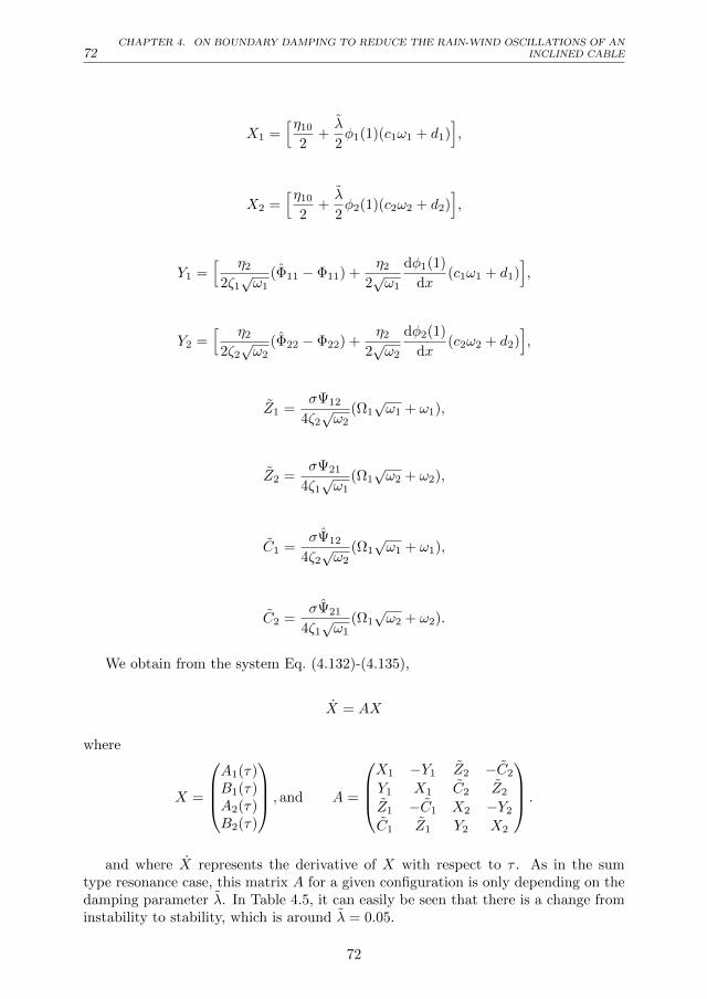
72CHAPTER 4. ON BOUNDARY DAMPING TO REDUCE THE RAIN-WIND OSCILLATIONS OF AN
INCLINED CABLE
X1 =[η10
2+λ
2φ1(1)(c1ω1 + d1)
],
X2 =[η10
2+λ
2φ2(1)(c2ω2 + d2)
],
Y1 =[ η2
2ζ1√ω1
(Φ11 − Φ11) +η2
2√ω1
dφ1(1)
dx(c1ω1 + d1)
],
Y2 =[ η2
2ζ2√ω2
(Φ22 − Φ22) +η2
2√ω2
dφ2(1)
dx(c2ω2 + d2)
],
Z1 =σΨ12
4ζ2√ω2
(Ω1√ω1 + ω1),
Z2 =σΨ21
4ζ1√ω1
(Ω1√ω2 + ω2),
C1 =σΨ12
4ζ2√ω2
(Ω1√ω1 + ω1),
C2 =σΨ21
4ζ1√ω1
(Ω1√ω2 + ω2).
We obtain from the system Eq. (4.132)-(4.135),
X = AX
where
X =
A1(τ)B1(τ)A2(τ)B2(τ)
, and A =
X1 −Y1 Z2 −C2
Y1 X1 C2 Z2
Z1 −C1 X2 −Y2
C1 Z1 Y2 X2
.
and where X represents the derivative of X with respect to τ . As in the sumtype resonance case, this matrix A for a given configuration is only depending on thedamping parameter λ. In Table 4.5, it can easily be seen that there is a change frominstability to stability, which is around λ = 0.05.
72
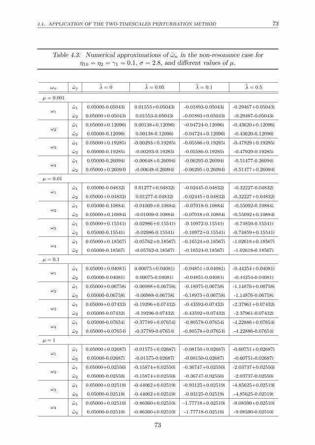
4.4. APPLICATION OF THE TWO-TIMESCALES PERTURBATION METHOD 73
Table 4.3: Numerical approximations of ωn in the non-resonance case forη10 = η2 = γ1 = 0.1, σ = 2.8, and different values of µ.
ωn ωj λ = 0 λ = 0.05 λ = 0.1 λ = 0.5
µ = 0.001
ω1ω1 0.05000-0.05043i 0.01553+0.05043i -0.01893-0.05043i -0.29467+0.05043i
ω2 0.05000+0.05043i 0.01553-0.05043i -0.01893+0.05043i -0.29467-0.05043i
ω2ω1 0.05000+0.12096i 0.00138+0.12096i -0.04724-0.12096i -0.43620+0.12096i
ω2 0.05000-0.12096i 0.00138-0.12096i -0.04724+0.12096i -0.43620-0.12096i
ω3ω1 0.05000+0.19285i -0.00293+0.19285i -0.05586+0.19285i -0.47929+0.19285i
ω2 0.05000-0.19285i -0.00293-0.19285i -0.05586-0.19285i -0.47929-0.19285i
ω4ω1 0.05000-0.26094i -0.00648+0.26094i -0.06295-0.26094i -0.51477-0.26094i
ω2 0.05000+0.26094i -0.00648-0.26094i -0.06295+0.26094i -0.51477+0.26094i
µ = 0.01
ω1ω1 0.05000-0.04832i 0.01277+0.04832i -0.02445-0.04832i -0.32227-0.04832i
ω2 0.05000+0.04832i 0.01277-0.04832i -0.02445+0.04832i -0.32227+0.04832i
ω2ω1 0.05000-0.10884i -0.01009+0.10884i -0.07018-0.10884i -0.55092-0.10884i
ω2 0.05000+0.10884i -0.01009-0.10884i -0.07018+0.10884i -0.55092+0.10884i
ω3ω1 0.05000+0.15541i -0.02986+0.15541i -0.10972-0.15541i -0.74859-0.15541i
ω2 0.05000-0.15541i -0.02986-0.15541i -0.10972+0.15541i -0.74859+0.15541i
ω4ω1 0.05000+0.18567i -0.05762+0.18567i -0.16524+0.18567i -1.02618+0.18567i
ω2 0.05000-0.18567i -0.05762-0.18567i -0.16524-0.18567i -1.02618-0.18567i
µ = 0.1
ω1ω1 0.05000+0.04081i 0.00075+0.04081i -0.04851+0.04081i -0.44254+0.04081i
ω2 0.05000-0.04081i 0.00075-0.04081i -0.04851-0.04081i -0.44254-0.04081i
ω2ω1 0.05000+0.06758i -0.06988+0.06758i -0.18975-0.06758i -1.14876+0.06758i
ω2 0.05000-0.06758i -0.06988-0.06758i -0.18975+0.06758i -1.14876-0.06758i
ω3ω1 0.05000+0.07432i -0.19296+0.07432i -0.43592-0.07432i -2.37961+0.07432i
ω2 0.05000-0.07432i -0.19296-0.07432i -0.43592+0.07432i -2.37961-0.07432i
ω4ω1 0.05000-0.07654i -0.37789+0.07654i -0.80578-0.07654i -4.22886+0.07654i
ω2 0.05000+0.07654i -0.37789-0.07654i -0.80578+0.07654i -4.22886-0.07654i
µ = 1
ω1ω1 0.05000+0.02687i -0.01575+0.02687i -0.08150+0.02687i -0.60751+0.02687i
ω2 0.05000-0.02687i -0.01575-0.02687i -0.08150-0.02687i -0.60751-0.02687i
ω2ω1 0.05000+0.02550i -0.15874+0.02550i -0.36747+0.02550i -2.03737+0.02550i
ω2 0.05000-0.02550i -0.15874+0.02550i -0.36747-0.02550i -2.03737-0.02550i
ω3ω1 0.05000+0.02519i -0.44062+0.02519i -0.93125+0.02519i -4.85625+0.02519i
ω2 0.05000-0.02519i -0.44062+0.02519i -0.93125-0.02519i -4.85625-0.02519i
ω4ω1 0.05000+0.02510i -0.86360+0.02510i -1.77718+0.02510i -9.08590+0.02510i
ω2 0.05000-0.02510i -0.86360+0.02510i -1.77718-0.02510i -9.08590-0.02510i
73

74CHAPTER 4. ON BOUNDARY DAMPING TO REDUCE THE RAIN-WIND OSCILLATIONS OF AN
INCLINED CABLE
Table 4.4: Numerical approximations of ωn in the sum type resonance case forη10 = η2 = γ1 = 0.1, σ = 2.8, and different values of µ.
ω λ = 0 λ = 0.05 λ = 0.1 λ = 0.5
µ = 0.001
ω1 0.04845+0.11079i 0.01800+0.04043i -0.05054+0.11145i -0.44189+0.11611i
ω2 0.04845-0.11079i 0.01800-0.04043i -0.01564+0.04085i -0.44189-0.11611i
ω3 0.05155+0.04017i -0.00109+0.11104i -0.01564-0.04085i -0.28898+0.04557i
ω4 0.05155-0.04017i -0.00109-0.11104i -0.05054-0.11145i -0.28898-0.04557i
µ = 0.01
ω1 0.04786+0.09626i 0.01689+0.03638i -0.07576+0.09834i -0.31627+0.04557i
ω2 0.04786-0.09626i 0.01689-0.03638i -0.07576-0.09834i -0.31627-0.04557i
ω3 0.05214+0.03554i -0.01421+0.09705i -0.01887+0.03772i -0.55691+0.10610i
ω4 0.05214-0.03554i -0.01421-0.09705i -0.01887-0.03772i -0.55691-0.10610i
µ = 0.1
ω1 0.03514+0.02827i 0.01955+0.02646i -0.03344+0.03425i -0.43828+0.04090i
ω2 0.03514-0.02827i 0.01955-0.02646i -0.03344-0.03425i -0.43828-0.04090i
ω3 0.07761+0i -0.08868+0.05346i -0.20482+0.06108i -1.15302+0.06767i
ω4 0.05210-0i -0.08868-0.05346i -0.20482-0.06108i -1.15302-0.06767i
µ = 1
ω1 0.15268+0.00330i 0.03971+0.02213i -0.04650+0.02694i -0.59965+0.02800i
ω2 0.15268-0.00330i 0.03971-0.02213i -0.04650-0.02694i -0.59965-0.02800i
ω3 -0.04855-0i -0.21419+0.02066i -0.40248+0.02553i -2.04522+0.02662i
ω4 -0.05682-0i -0.21419-0.02066i -0.40248-0.02553i -2.04522-0.02662i
74
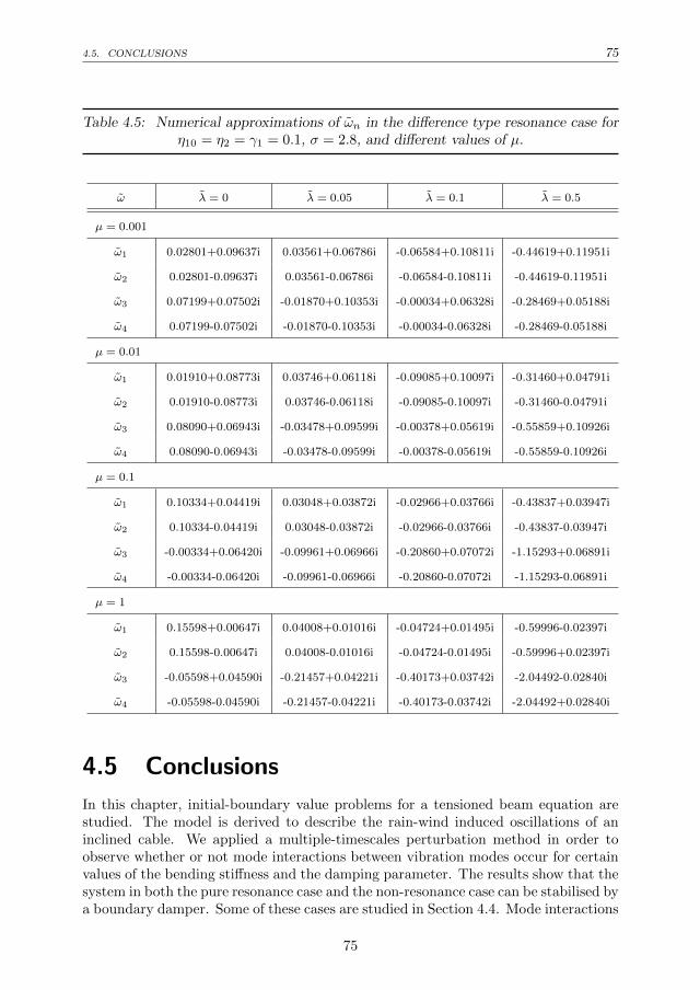
4.5. CONCLUSIONS 75
Table 4.5: Numerical approximations of ωn in the difference type resonance case forη10 = η2 = γ1 = 0.1, σ = 2.8, and different values of µ.
ω λ = 0 λ = 0.05 λ = 0.1 λ = 0.5
µ = 0.001
ω1 0.02801+0.09637i 0.03561+0.06786i -0.06584+0.10811i -0.44619+0.11951i
ω2 0.02801-0.09637i 0.03561-0.06786i -0.06584-0.10811i -0.44619-0.11951i
ω3 0.07199+0.07502i -0.01870+0.10353i -0.00034+0.06328i -0.28469+0.05188i
ω4 0.07199-0.07502i -0.01870-0.10353i -0.00034-0.06328i -0.28469-0.05188i
µ = 0.01
ω1 0.01910+0.08773i 0.03746+0.06118i -0.09085+0.10097i -0.31460+0.04791i
ω2 0.01910-0.08773i 0.03746-0.06118i -0.09085-0.10097i -0.31460-0.04791i
ω3 0.08090+0.06943i -0.03478+0.09599i -0.00378+0.05619i -0.55859+0.10926i
ω4 0.08090-0.06943i -0.03478-0.09599i -0.00378-0.05619i -0.55859-0.10926i
µ = 0.1
ω1 0.10334+0.04419i 0.03048+0.03872i -0.02966+0.03766i -0.43837+0.03947i
ω2 0.10334-0.04419i 0.03048-0.03872i -0.02966-0.03766i -0.43837-0.03947i
ω3 -0.00334+0.06420i -0.09961+0.06966i -0.20860+0.07072i -1.15293+0.06891i
ω4 -0.00334-0.06420i -0.09961-0.06966i -0.20860-0.07072i -1.15293-0.06891i
µ = 1
ω1 0.15598+0.00647i 0.04008+0.01016i -0.04724+0.01495i -0.59996-0.02397i
ω2 0.15598-0.00647i 0.04008-0.01016i -0.04724-0.01495i -0.59996+0.02397i
ω3 -0.05598+0.04590i -0.21457+0.04221i -0.40173+0.03742i -2.04492-0.02840i
ω4 -0.05598-0.04590i -0.21457-0.04221i -0.40173-0.03742i -2.04492+0.02840i
4.5 Conclusions
In this chapter, initial-boundary value problems for a tensioned beam equation arestudied. The model is derived to describe the rain-wind induced oscillations of aninclined cable. We applied a multiple-timescales perturbation method in order toobserve whether or not mode interactions between vibration modes occur for certainvalues of the bending stiffness and the damping parameter. The results show that thesystem in both the pure resonance case and the non-resonance case can be stabilised bya boundary damper. Some of these cases are studied in Section 4.4. Mode interactions
75
76CHAPTER 4. ON BOUNDARY DAMPING TO REDUCE THE RAIN-WIND OSCILLATIONS OF AN
INCLINED CABLE
between two and more modes depending on the bending stiffness µ are possible.More complicated resonance cases can be Ω1 =
√ωn ±
√ωm or Ω1 = 2
√ωn, when
Ω1 =√ωN +
√ωM ( or Ω1 =
√ωN−
√ωM ) for some fixed N and M . These cases still
have to be studied, and can be studied by using the techniques as shown in Section4.4 of this chapter.
This chapter provides an understanding of how effective boundary damping canbe for the in-plane transversal oscillations of the cable. The same approach can beused for in-plane and out-of-plane transversal oscillations of elastic structures.
76

Appendix AAerodynamic parameters
b := [−(ψ1 + α1) + arctan(tan(γ))], (A.1)
c := [−(ψ2 + α2) + arctan(tan(γ))], (A.2)
a000 := sin(γ), (A.3)
a001 := b cos(γ), (A.4)
a002 := c cos(γ), (A.5)
a003 := b3cos(γ), (A.6)
a004 := c3cos(γ), (A.7)
a100 := 2− cos2(γ), (A.8)
a101 := cos(γ)[cos(γ)− b sin(γ)], (A.9)
a102 := cos(γ)[cos(γ)− c sin(γ)], (A.10)
a103 := b2cos(γ)[3cos(γ)− b sin(γ)], (A.11)
a104 := c2cos(γ)[3cos(γ)− c sin(γ)], (A.12)
a010 := −sin(γ)cos(γ), (A.13)
a011 := sin(γ)[cos(γ)− b sin(γ)], (A.14)
a012 := sin(γ)[cos(γ)− c sin(γ)], (A.15)
a013 := b2sin(γ)[3cos(γ)− b sin(γ)], (A.16)
a014 := c2sin(γ)[3cos(γ)− c sin(γ)], (A.17)
a200 :=sin(γ)
2[2 + cos2(γ)], (A.18)
a201 :=cos(γ)
2[2b− 3b cos2(γ)− 2 sin(2γ)], (A.19)
a202 :=cos(γ)
2[2c− 3c cos2(γ)− 2 sin(2γ)], (A.20)
77
78 APPENDIX A. AERODYNAMIC PARAMETERS
a203 :=b cos(γ)
2[2b2 + cos2(γ)(6− 3b2)− 6b sin(2γ)], (A.21)
a204 :=c cos(γ)
2[2c2 + cos2(γ)(6− 3c2)− 6c sin(2γ)], (A.22)
a110 := cos3(γ), (A.23)
a111 := 4cos3(γ)− 3cos(γ) + b[sin(γ)− 3sin(γ)cos2(γ)], (A.24)
a112 := 4cos3(γ)− 3cos(γ) + c[sin(γ)− 3sin(γ)cos2(γ)], (A.25)
a113 := 6bsin(γ)cos2(γ) + b2[12cos3(γ)− 9cos(γ)] + b3[−3sin(γ)cos2(γ) + sin(γ)],(A.26)
a114 := 6csin(γ)cos2(γ) + c2[12cos3(γ)− 9cos(γ)] + c3[−3sin(γ)cos2(γ) + sin(γ)],(A.27)
a020 := − sin(γ)
2[3 + cos2(γ)], (A.28)
a021 := 2sin(γ)cos2(γ)− sin(γ)− 3b
2sin2(γ)cos(γ), (A.29)
a022 := 2sin(γ)cos2(γ)− sin(γ)− 3c
2sin2(γ)cos(γ), (A.30)
a023 := 3b sin2(γ)cos(γ) + b2[6 sin(γ)cos2(γ)− 3 sin(γ)]− 3b3
2sin2(γ)cos(γ), (A.31)
a024 := 3c sin2(γ)cos(γ) + c2[6 sin(γ)cos2(γ)− 3 sin(γ)]− 3c3
2sin2(γ)cos(γ), (A.32)
a300 :=cos2(γ)
2[5 cos2(γ)− 4], (A.33)
a301 := −cos(γ)
6[−15b sin(γ)cos2(γ) + 23 cos3(γ) + 6b sin(γ)− 18 cos(γ)], (A.34)
a302 := −cos(γ)
6[−15c sin(γ)cos2(γ) + 23 cos3(γ) + 6c sin(γ)− 18 cos(γ)], (A.35)
a303 :=(
1− 23b2
2
)cos4(γ) +
(5b3
2− 9b
)sin(γ)cos3(γ) + 9b2 cos2(γ)− b3 sin(γ)cos(γ),
(A.36)
a304 :=(
1− 23c2
2
)cos4(γ) +
(5c3
2− 9c
)sin(γ)cos3(γ) + 9c2 cos2(γ)− c3 sin(γ)cos(γ),
(A.37)
a210 :=3
2sin(γ)cos3(γ), (A.38)
a211 := b [15
2cos2(γ)− 15
2cos4(γ)− 1] + 5sin(γ)cos(γ)− 23
2sin(γ)cos3(γ), (A.39)
a212 := c [15
2cos2(γ)− 15
2cos4(γ)− 1] + 5sin(γ)cos(γ)− 23
2sin(γ)cos3(γ), (A.40)
a213 :=(
27b− 15b3
2
)cos4(γ) +
(3− 69b2
2
)sin(γ)cos3(γ) (A.41)
+(15b3
2− 21b
)cos2(γ) + 15b2sin(γ)cos(γ)− b3,
78

79
a214 :=(
27c− 15c3
2
)cos4(γ) +
(3− 69c2
2
)sin(γ)cos3(γ) (A.42)
+(15c3
2− 21c
)cos2(γ) + 15c2sin(γ)cos(γ)− c3,
a120 :=3
2sin2(γ)cos2(γ), (A.43)
a121 := b(− 15
2sin(γ)cos3(γ) +
9
2sin(γ)cos(γ)
)+
17
2cos4(γ)− 19
2cos2(γ) + 2, (A.44)
a122 := c(− 15
2sin(γ)cos3(γ) +
9
2sin(γ)cos(γ)
)+
17
2cos4(γ)− 19
2cos2(γ) + 2, (A.45)
a123 :=(51b2
2− 3)
cos4(γ) +(
27b− 15b3
2
)sin(γ)cos3(γ) (A.46)
+(
3− 57b2
2
)cos2(γ) +
(9b3
2− 15b
)sin(γ)cos(γ) + 6b2,
a124 :=(51c2
2− 3)
cos4(γ) +(
27c− 15c3
2
)sin(γ)cos3(γ) (A.47)
+(
3− 57c2
2
)cos2(γ) +
(9c3
2− 15c
)sin(γ)cos(γ) + 6c2,
a030 :=1
2sin3(γ)cos(γ), (A.48)
a031 :=sin(γ)
6[23 cos3(γ)− 17 cos(γ)] +
b sin2(γ)
2[1− 5 cos2(γ)], (A.49)
a032 :=sin(γ)
6[23 cos3(γ)− 17 cos(γ)] +
c sin2(γ)
2[1− 5 cos2(γ)], (A.50)
a033 :=(23b2
2− 1)
cos3(γ)sin(γ)−(5b3
2− 9b
)sin2(γ)cos2(γ) (A.51)
+(
1− 17b2
2
)sin(γ)cos(γ) +
(b32− 3b
)sin2(γ),
a034 :=(23c2
2− 1)
cos3(γ)sin(γ)−(5c3
2− 9c
)sin2(γ)cos2(γ) (A.52)
+(
1− 17c2
2
)sin(γ)cos(γ) +
(c32− 3c
)sin2(γ),
b000 := cos(γ), (A.53)
b001 := b sin(γ), (A.54)
b002 := c sin(γ), (A.55)
b003 := b3sin(γ), (A.56)
b004 := c3sin(γ), (A.57)
79

80 APPENDIX A. AERODYNAMIC PARAMETERS
b100 := sin(γ)cos(γ), (A.58)
b101 := cos(γ)[b cos(γ) + sin(γ)], (A.59)
b102 := cos(γ)[c cos(γ) + sin(γ)], (A.60)
b103 := b2cos(γ)[3sin(γ) + b cos(γ)], (A.61)
b104 := c2cos(γ)[3sin(γ) + c cos(γ)], (A.62)
b010 := −1− cos2(γ), (A.63)
b011 := sin(γ)[b cos(γ) + sin(γ)], (A.64)
b012 := sin(γ)[c cos(γ) + sin(γ)], (A.65)
b013 := b2sin(γ)[3sin(γ) + b cos(γ)], (A.66)
b014 := c2sin(γ)[3sin(γ) + c cos(γ)], (A.67)
b200 :=cos3(γ)
2, (A.68)
b201 := −cos(γ)
2[2− 4 cos2(γ) + 3b sin(γ)cos(γ)], (A.69)
b202 := −cos(γ)
2[2− 4 cos2(γ) + 3c sin(γ)cos(γ)], (A.70)
b203 :=−3b
2cos(γ)[b2 sin(γ)cos(γ)− 4b cos2(γ)− 2sin(γ)cos(γ) + 2b], (A.71)
b204 :=−3c
2cos(γ)[c2 sin(γ)cos(γ)− 4c cos2(γ)− 2sin(γ)cos(γ) + 2c], (A.72)
b110 := −sin3(γ), (A.73)
b111 := b [3cos3(γ)− 2cos(γ)] + 4sin(γ)cos2(γ)− sin(γ), (A.74)
b112 := c [3cos3(γ)− 2cos(γ)] + 4sin(γ)cos2(γ)− sin(γ), (A.75)
b113 := b3 [3cos3(γ)− 2cos(γ)] + 3b2 [4cos2(γ)sin(γ)− sin(γ)]− 6b[cos3(γ)− cos(γ)],(A.76)
b114 := c3 [3cos3(γ)− 2cos(γ)] + 3c2 [4cos2(γ)sin(γ)− sin(γ)]− 6c[cos3(γ)− cos(γ)],(A.77)
b020 := −cos(γ)
2[cos2(γ)− 3], (A.78)
b021 :=sin(γ)
2[3b cos2(γ) + 4sin(γ)cos(γ)− b], (A.79)
b022 :=sin(γ)
2[3c cos2(γ) + 4sin(γ)cos(γ)− c], (A.80)
b023 :=b
2sin(γ)[3b2 cos2(γ) + 12b sin(γ)cos(γ)− 6cos2(γ)− b2 + 6], (A.81)
b024 :=c
2sin(γ)[3c2 cos2(γ) + 12c sin(γ)cos(γ)− 6cos2(γ)− c2 + 6], (A.82)
b300 := −1
2sin(γ)cos3(γ), (A.83)
80

81
b301 := −cos(γ)
6[3b cos3(γ) + 23 sin(γ)cos2(γ)− 6sin(γ)], (A.84)
b302 := −cos(γ)
6[3c cos3(γ) + 23 sin(γ)cos2(γ)− 6sin(γ)], (A.85)
b303 :=(
9b− b3
2
)cos4(γ) +
(1− 23b2
2
)sin(γ)cos3(γ)− 6b cos2(γ) + 3b2 sin(γ)cos(γ),
(A.86)
b304 :=(
9c− c3
2
)cos4(γ) +
(1− 23c2
2
)sin(γ)cos3(γ)− 6c cos2(γ) + 3c2 sin(γ)cos(γ),
(A.87)
b210 := −3
2sin2(γ)cos2(γ), (A.88)
b211 := b[−15
2cos3(γ)sin(γ) + 3sin(γ)cos(γ)] +
19
2cos4(γ)− 17
2cos2(γ) + 1, (A.89)
b212 := c[−15
2cos3(γ)sin(γ) + 3sin(γ)cos(γ)] +
19
2cos4(γ)− 17
2cos2(γ) + 1, (A.90)
b213 :=(69b2
2− 3)
cos4(γ) +(
27b− 15b3
2
)cos3(γ)sin(γ) (A.91)
+(
3− 63b2
2
)cos2(γ) +
(3b3 − 12b
)cos(γ)sin(γ) + 3b2,
b214 :=(69c2
2− 3)
cos4(γ) +(
27c− 15c3
2
)cos3(γ)sin(γ) (A.92)
+(
3− 63c2
2
)cos2(γ) +
(3c3 − 12c
)cos(γ)sin(γ) + 3c2,
b120 := −3
2cos(γ)sin3(γ), (A.93)
b121 := b[15
2cos4(γ)− 15
2cos2(γ) + 1] +
23
2cos3(γ)sin(γ)− 13
2cos(γ)sin(γ), (A.94)
b122 := c[15
2cos4(γ)− 15
2cos2(γ) + 1] +
23
2cos3(γ)sin(γ)− 13
2cos(γ)sin(γ), (A.95)
b123 :=(15b3
2− 27b
)cos4(γ) +
(69b2
2− 3)
cos3(γ)sin(γ) (A.96)
+(
33b− 15b3
2
)cos2(γ) +
(3− 39b2
2
)cos(γ)sin(γ) + b3 − 6b,
b124 :=(15c3
2− 27c
)cos4(γ) +
(69c2
2− 3)
cos3(γ)sin(γ) (A.97)
+(
33c− 15c3
2
)cos2(γ) +
(3− 39c2
2
)cos(γ)sin(γ) + c3 − 6c,
b030 := − sin2(γ)
2[cos2(γ)− 2cos(γ) + 1], (A.98)
81
82 APPENDIX A. AERODYNAMIC PARAMETERS
b031 :=sin(γ)
6[15b cos3(γ) + 23 cos2(γ)sin(γ)− 9b cos(γ)− 5sin(γ)], (A.99)
b032 :=sin(γ)
6[15c cos3(γ) + 23 cos2(γ)sin(γ)− 9c cos(γ)− 5sin(γ)], (A.100)
b033 :=(5b3
2− 9b
)cos3(γ)sin(γ) +
(23b2
2− 1)
cos2(γ)sin2(γ) (A.101)
+(
9b− 3b3
2
)sin(γ)cos(γ) +
(1− 5b2
2
)sin2(γ),
b034 :=(5c3
2− 9c
)cos3(γ)sin(γ) +
(23c2
2− 1)
cos2(γ)sin2(γ) (A.102)
+(
9c− 3c3
2
)sin(γ)cos(γ) +
(1− 5c2
2
)sin2(γ).
82
Appendix BStationary Solution ux and vx
The stationary solution follows from Eq. (4.33) and (4.34) by considering no time-dependence, yielding
− EM
∂
∂x
(ux +
v2x
2
)=[A γ1 cos(γ1x− Ω1t)
]g sin(α)x (B.1)
+[2 + 2A sin(γ1x− Ω1t)
]g sin(α),
EIyAM
vxxxx −T0
AMvxx −
E
M
∂
∂x
[vx
(ux +
v2x
2
)]=[A γ1 cos(γ1x− Ω1t)
]g sin(α)xvx
(B.2)
+[1 + A sin(γ1x− Ω1t)
]g sin(α)xvxx
+[1 + A sin(γ1x− Ω1t)
]g sin(α)vx
+[1 + A sin(γ1x− Ω1t)
]g cos(α)
− ρa2AM
dLv2∞A00.
It will be assumed that u is O(ε2), v is O(ε), A is O(ε), gsin(α) = P ∗0 is O(1),EM = P ∗1 is O(1/ε),
EIyAM = P ∗2 is O(1/ε), and T0
AM = P ∗3 is O(1/ε), where ε is a smallparameter with 0 < ε 1. Then, by using these assumptions, Eq. (B.1) and (B.2)becomes
−P ∗1∂
∂x
(ux +
v2x
2
)= 2g sin(α) +O(ε), (B.3)
P ∗2 vxxxx−P ∗3 vxx−P ∗1∂
∂x
[vx
(ux+
v2x
2
)]=
∂
∂x
[P ∗0 xvx
]+g cos(α)− ρa
2AMdLv2
∞A00+O(ε).
(B.4)
83
84 APPENDIX B. STATIONARY SOLUTION UX AND VX
with the boundary conditions
u(L) = u(0) = 0, (B.5)
v(0) = vxx(0) = vx(L) = 0,
EIy vxxx(L) = [T0 +AMLgsin(α)]vx(L).
When Eq. (B.3) and (B.4) are integrated with respect to x, we may rewrite(ux +
v2x
2
)= −2g sin(α)x
P ∗1+ k1, (B.6)
vxxx−P ∗3P ∗2
vxx−P ∗1P ∗2
∂
∂x
[vx
(ux+
v2x
2
)]=P ∗0P ∗2
xvx+g cos(α)x
P ∗2− ρa
2AMP ∗2dLv2
∞A00x+k2,
(B.7)where k1 and k2 are constants of integration. Substitute Eq. (B.6) into Eq. (B.7), weobtain
vxxxx − vx(k3 − xk4) = k2 + xk5, (B.8)
where k3 = T0
EIy+ k1
AIy
, k4 =P∗0P∗2
, and k5 =P∗0P∗2− ρa
2AMP∗2dLv2
∞A00. In order to
solve the non-homogeneous PDE Eq. (B.8), we will apply the method of variation ofparameters and obtain
v(x) =
∫ x
0
C1Ai
(k3 − xk4
k2/34
)dx+
∫ x
0
C2Bi
(k3 − xk4
k2/34
)dx (B.9)
−∫ x
0
Ai
(k3 − xk4
k2/34
)∫ x
0
(k2 + sk5
Wr(s)
)Bi
(k3 − sk4
k2/34
)ds
dx
+
∫ x
0
Bi
(k3 − xk4
k2/34
)∫ x
0
(k2 + sk5
Wr(s)
)Ai
(k3 − sk4
k2/34
)ds
dx+ C3.
Here Ai and Bi are Airy functions, and C1, C2 and C3 are constants of integration,and
Wr(x) = Ai
(k3 − xk4
k2/34
) d
dx
[Bi
(k3 − xk4
k2/34
)]−Bi
(k3 − xk4
k2/34
) d
dx
[Ai
(k3 − xk4
k2/34
)].
(B.10)Substituting Eq. (B.9) into Eq. (B.6) and integrated with respect to x, we obtain
u(x) =−∫ x
0
( 2g
P ∗1sin(α) x+ k1
)dx+ C4 (B.11)
− 1
2
∫ x
0
C1Ai
(k3 − xk4
k2/34
)+ C2Bi
(k3 − xk4
k2/34
)−Ai
(k3 − xk4
k2/34
)[ ∫ x
0
(k2 + sk5
Wr(s)
)Bi
(k3 − sk4
k2/34
)ds]
+Bi
(k3 − xk4
k2/34
)[ ∫ x
0
(k2 + sk5
Wr(s)
)Ai
(k3 − sk4
k2/34
)ds]2
dx.
84
85
where C4 is a constant of integration. By satisfying boundary conditions Eq. (B.5)for stationary solution, we obtain
k1 :=g sin(α)L
P ∗1+
1
2L
∫ L
0
v2xdx, (B.12)
k2 :=N3F1 − F3N1
N1F2 + F1N2, (B.13)
C1 := −C2
Bi
(1, k3
k2/34
)Ai
(1, k3
k2/34
) , (B.14)
C2 :=N3F2 + F3N2
N1F2 + F1N2, (B.15)
C3 := C4 = 0, (B.16)
where
N1 :=
−Ai
(k3 − Lk4
k2/34
)Bi(1, k3k2/34
)Ai
(1, k3
k2/34
) +Bi
(k3 − Lk4
k2/34
), (B.17)
N2 :=
−Ai
(k3 − Lk4
k2/34
)∫ L
0
1
Wr(x)Bi
(k3 − xk4
k2/34
)dx (B.18)
+Bi
(k3 − Lk4
k2/34
)∫ L
0
1
Wr(x)Ai
(k3 − xk4
k2/34
)dx
,
N3 :=
Ai
(k3 − Lk4
k2/34
)∫ L
0
xk5
Wr(x)Bi
(k3 − xk4
k2/34
)dx (B.19)
−Bi(k3 − Lk4
k2/34
)∫ L
0
xk5
Wr(x)Ai
(k3 − xk4
k2/34
)dx
,
F1 :=EIy
[T0 +AMLgsin(α)](k3 −Lk4)
Bi
(k3 − Lk4
k2/34
)−Ai
(k3 − Lk4
k2/34
)Bi(1, k3k2/34
)Ai
(1, k3
k2/34
),(B.20)
85

86 APPENDIX B. STATIONARY SOLUTION UX AND VX
F2 :=EIy
[T0 +AMLgsin(α)](k3 − Lk4)
Ai
(k3 − Lk4
k2/34
)∫ L
0
1
Wr(x)Bi
(k3 − xk4
k2/34
)dx
(B.21)
−Bi(k3 − Lk4
k2/34
)∫ L
0
1
Wr(x)Ai
(k3 − xk4
k2/34
)dx
+EIyT0
k1/34
Ai
(1,k3 − Lk4
k2/34
) 1
Wr(L)Bi
(k3 − Lk4
k2/34
)−Bi
(1,k3 − Lk4
k2/34
) 1
Wr(L)Ai
(k3 − Lk4
k2/34
),
F3 :=EIy
[T0 +AMLgsin(α)](k3 − Lk4)
Ai
(k3 − Lk4
k2/34
)∫ L
0
xk5
Wr(x)Bi
(k3 − xk4
k2/34
)dx
(B.22)
−Bi(k3 − Lk4
k2/34
)∫ L
0
xk5
Wr(x)Ai
(k3 − xk4
k2/34
)dx
+EIyT0
k1/34
−Ai
(1,k3 − Lk4
k2/34
) Lk5
Wr(L)Bi
(k3 − Lk4
k2/34
)+Bi
(1,k3 − Lk4
k2/34
) Lk5
Wr(L)Ai
(k3 − Lk4
k2/34
).
86
Bibliography
[1] A. K. Abramian and S. A. Vakulenko. Oscillations of a beam with a time-varyingmass. Nonlinear Dynamics, 63(1-2):135–147, 2011.
[2] A.K. Abramian, W.T. van Horssen, and S.A Vakulenko. Nonlinear vibrations ofa beam with time-varying rigidity and mass. Nonlinear Dynamics, 71(1-2):291–312, 2013.
[3] A.K. Abramian, W.T. van Horssen, and S.A Vakulenko. On oscillations of a beamwith a small rigidity and a time-varying mass. Nonlinear Dynamics, 78:449–459,2014.
[4] T. Akkaya and W.T. van Horssen. Reflection and damping properties for semi-infinite string equations with non-classical boundary conditions. Journal ofSound and Vibration, 336(3):179–190, 2015.
[5] Tugce Akkaya and Wim T. van Horssen. On constructing a green’s function fora semi-infinite beam with boundary damping. Meccanica, pages 1–13, 2016.
[6] S.V. Alekseenko, D.M. Markovich, V.E. Nakoryakovand, and S.I. Shtork. Rivuletflow of liquid on the outer surface of an inclined cylinder. Journal of AppliedMechanics and Technical Physics, 38(4):649–653, 1998.
[7] H. Bateman. Tables of Integral Transforms, Volume 1. McGraw-Hill Book Com-pany , Inc., New York, 1954.
[8] G. J. Boertjens and W. T. van Horssen. On interactions of oscillation modes fora weakly non-linear undamped elastic beam with an external force. Journal ofSound and Vibration, 235(2):201–217, 2000.
[9] W.E. Boyce and R.C. DiPrima. Elementary Differential Equations and BoundaryValue Problems. John Wiley & Sons, Inc., New York, 2005.
[10] A.H.P. Van Der Burgh, Hartono, and A.K. Abramian. A new model for the studyof rain-wind-induced vibrations of a simple oscillator. International Journal ofNon-Linear Mechanics, 41(3):345–358, 2006.
87

88 BIBLIOGRAPHY
[11] P. C. van Staalduinen C. P. W. Geurts. Estimation of the effects of rain-windinduced vibration in the design stage of inclined stay cables. In Proceedings 10thInternational Conference on Wind Engineering, Copenhagen, June 1999.
[12] G. A. Campbell and R. M. Foster. Fourier Integrals for Practical Applications.Bell Telephone Laboratories, New York, 1931.
[13] Caswita. On the dynamics of an inclined stretched string. PhD thesis, DelftUniversity of Technology, 2004.
[14] Caswita. On the dynamics of an inclined stretched string. PhD thesis, DelftUniversity of Technology, 2004.
[15] S. Colombo and J. Lavoine. Transformations de Laplace et de Mellin. Gauthier-Villars, Paris, 1972.
[16] F. Conrad and O. Morgul. On the stabilization of a flexible beam with a tipmass. SIAM J. Control Optim., 36(6):1962–1986, November 1998.
[17] L. Cremer. Physics of the Violin. MIT Press, Cambridge, 1981.
[18] Darmawijoyo. n the vibrations of a linear and a weakly 1-d wave equations withnon-classical boundary damping. Journal of Applied Sciences, 11:1206–1212,2011.
[19] Darmawijoyo and W. T. van Horssen. On the weakly damped vibrations ofa string attached to a spring-mass-dashpot system. Journal of Vibration andControl, 9(11):1231–1248, 2003.
[20] N. V. Gaiko and W. T. van Horssen. On the transverse, low frequency vibrationsof a traveling string with boundary damping. Journal of Vibration and Acoustics,137(4):041004–041004–10, 2015.
[21] C. Geurts, T. Vrouwenvelder, P. van Staalduinen, and J. Reusink. Numericalmodelling of rain-wind-induced vibration: Erasmus bridge, rotterdam. StructuralEngineering International, 8(2):129–135, May 1998.
[22] C. Geurts, T. Vrouwenvelder, P. van Staalduinen, and J. Reusink. Riesz basisapproach to the stabilization of a flexible beam with a tip mass. SIAM J. ControlOptim., 39(6):1736–1747, 2001.
[23] K. Girkmann. Flachentragwerke. Springer, Wien, 1963.
[24] H. Goldstein. Classical Mechanics. Addison-Wisley Publ. Co., Singapore, 1980.
[25] K.F. Graff. Wave Motion in Elastic Solids. Clarendon Press, Oxford, 1975.
[26] R.B. Guenther and J.W. Lee. Partial Differential Equations of MathematicalPhysics and Integral Equations. Prentice-Hall, New Jersey, 1988.
[27] R. Haberman. Applied Partial Differential Equations. Pearson Prentice-Hall,New Jersey, 2004.
88
BIBLIOGRAPHY 89
[28] J. W. Hijmissen. On aspects of boundary damping for cables and vertical beams.Ph.D thesis, Delft University of Technology, Delft, The Netherlands, 2008.
[29] J. W. Hijmissen and W. T. van Horssen. On aspects of damping for a verticalbeam with a tuned mass damper at the top. Nonlinear Dynamics, 50(1-2):169–190, 2007.
[30] J.W. Hijmissen, N.W. van den Heuvel, and W.T. van Horssen. On the effectof the bending stiffness on the damping properties of a tensioned cable with anattached tuned-mass-damper. Engineering Structures, 31(5):1276–1285, 2009.
[31] Y. Hikami and N. Shiraishi. Rain-wind induced vibrations of cables stayedbridges. Journal of Wind Engineering and Industrial Aerodynamics, 29(1-3):409–418, 1988.
[32] D. J. Inman. Engineering Vibration. Prentice Hal, New Jersey, 2007.
[33] H. Irschik and H. Holl. Mechanics of variable-mass systems-part 1: Balance ofmass and linear momentum. Applied Mechanics Reviews, Transactions of theASME, 57(2):145–160, April 2004.
[34] Raymond G. Jacquot. Optimal damper location for randomly forced cantileverbeams. Journal of Sound and Vibration, 269(3–5):623 – 632, 2004.
[35] A. Jerri. Introduction to integral equations with applications. John Wiley & Sons,Inc., New York, 1999.
[36] I. Karnovsky and O. Lebed. Free Vibrations of Beams and Frames : Eigenvaluesand Eigenfuctions. McGraw-Hill Professional, 2004.
[37] H. Kauderer. Nichtlineare Mechanik. Springer-Verlag, Berlin, 1958.
[38] Sjors Kole. On the rain-wind induced vibrations of a mass-spring system. Mas-ter’s thesis, Delft University of Technology, 2016.
[39] X. Liu, B. Huo, and S. Zhang. Nonlinear dynamic analysis on the rain-wind-induced vibration of cable considering the equilibrium position of rivulet. Abstractand Applied Analysis, 2013(Article ID 927632):10 pages, 2013.
[40] A. Luongo and D. Zulli. Dynamic instability of inclined cables under combinedwind flow and support motion. Nonlinear Dynamics, 67(1):71–87, 2012.
[41] J. A. Main and N. P. Jones. Vibration of tensioned beams with intermediatedamper. i: Formulation, influence of damper location. Journal of EngineeringMechanics, 133(4):369–378, 2007.
[42] J. A. Main and N. P. Jones. Vibration of tensioned beams with intermedi-ate damper. ii: Damper near a support. Journal of Engineering Mechanics,133(4):379–388, 2007.
[43] Pramod Malatkar. Nonlinear Vibrations of Cantilever Beams and Plates. PhDthesis, Virginia Polytechnic Institute and State University, 2003.
89

90 BIBLIOGRAPHY
[44] P. J. McKenna and W. Walter. Travelling waves in a suspension bridge. SIAMJournal on Applied Mathematics, 50(3):703–715, 1990.
[45] W. L. Miranker. The wave equation in a medium in motion. IBM Journal ofResearch and Development, 4(1):36–42, January 1960.
[46] O. Morgul, B. P. Rao, and F. Conrad. On the stabilization of a cable with a tipmass. IEEE Trans. Autom. Control, 39:2140–2145, 1994.
[47] P.M. Morse and H. Feshbach. Methods of Theoretical Physics. McGraw-Hill,New York, 1953.
[48] F. Oberhettinger and L. Badii. Tables of Laplace Transformations. Springer,Berlin, 1973.
[49] N. Ortner. The initial-boundary value problem of the transverse vibrations ofa homogeneous beam clamped at one end and infinitely long in one direction.Bulletin of the Polish Academy of Sciences Mathematics, 26:389–415, 1978.
[50] N. Ortner and P. Wagner. The green’s functions of clamped semi-infinite vibrat-ing beams and plates. International Journal of Solids and Structures, 26(2):237–249, 1990.
[51] A. D. Polyanin. Handbook of Linear Partial Differential Equations for Engineersand Scientists. CRC Press, New York, 2002.
[52] S. H. Sandilo and W. T. van Horssen. On boundary damping for an axiallymoving tensioned beam. Journal of Vibration and Acoustics, Transactions of theASME, 124(1):11005, February 2012.
[53] T. L. Schmitz and K. S. Smith. Mechanical Vibrations: Modeling and Measure-ment. Springer New York, 2011.
[54] N. Srinil, G. Rega, and S. Chucheepsakul. Large amplitude three-dimensional freevibrations of inclined sagged elastic cables. Nonlinear Dynamics, 33(2):129–154,2003.
[55] I. Todhunter and K. Pearson. A History of the Theory of Elasticity and ofthe Strenght of Materials: From Galilei to the Present Time, Volume 2. TheUniversity Press, Cambridge, 1893.
[56] W. T. van Horssen. Asymptotic theory for a class of initial-boundary valueproblems for weakly nonlinear wave equations with an application to a modelof the galloping oscillations of overhead transmission lines. SIAM Journal ofApplied Mathematics, 48(6):1227–11243, December 1988.
[57] W. T. van Horssen, A.K. Abramian, and Hartono. On the free vibrations of anoscillator with a periodically time-varying mass. Journal of Sound and Vibration,298(4-5):1166–1172, December 2006.
[58] W. T. van Horssen, O.V.Pischanskyy, and J.L.A. Dubbeldam. On the forcedvibrations of an oscillator with a periodically time-varying mass. Journal ofSound and Vibration, 329(6):721–732, 2010.
90

BIBLIOGRAPHY 91
[59] J. Woodhouse. On the playability of violins: Part 1 reflection functions. ActaAcustica united with Acustica, 78(3):125–136, April 1993.
[60] J. Woodhouse. On the playability of violins: Part 2 minimum bow force andtransients. Acta Acustica united with Acustica, 78(3):137–153, April 1993.
[61] H. Yamaguchi. Analytical study on growth mechanism of rain vibration of cables.Journal of Wind Engineering and Industrial Aerodynamics, 33:73–80, 1990.
[62] M. A. Zarubinskaya and W. T. van Horssen. Coupled torsional and verticaloscillations of a beam subjected to boundary damping. Journal of Sound andVibration, 298(4-5):1113–1128, December 2006.
91

92 BIBLIOGRAPHY
92
Summary
Many mathematical models, which describe oscillations in elastic structures such assuspension bridges, conveyor belts and elevator cables, can be formulated as initial-boundary value problems for string (wave) equations, or for beam equations. Inorder to build more durable, elegant and lighter mechanical structures, the undesiredvibrations can be suppressed by using dampers.
In this thesis, the effect of boundary damping on elastic structures is studied.In Chapter 2, as a simple model of oscillations of a cable, a semi-infinite string-like problem is modelled by an initial boundary value problem with (non)-classicalboundary conditions. We apply the classical method of D’Alembert to obtain theexact solution which provides information about the efficiency of the damper at theboundary.
In Chapter 3, initial-boundary value problems for a beam equation on a semi-infinite interval and on a finite interval have been studied. The method of Laplacetransforms is applied to obtain the Greens function for a transversally vibrating ho-mogeneous semi-infinite beam, and the exact solution for various boundary conditionsare examined. The analytical results confirm earlier obtained results, and are vali-dated by explicit numerical approximations of the damping and oscillating rates. Thestudy shows that the numerical results approximate the exact results for sufficientlylarge domain lengths and for a sufficiently high number of modes. Moreover, the studyprovides an understanding of how the Greens functions for a semi-infinite beam canbe computed analytically for (non)-classical boundary conditions.
Finally, in Chapter 4 the studies as presented in Chapter 2 and in Chapter 3 areextended to inclined structures. A model is derived to describe the rain-wind inducedoscillations of an inclined cable. For a linearly formulated initial-boundary valueproblem for a tensioned beam equation describing the in-plane transversal oscillationsof the cable, the effectiveness of a boundary damper is determined by using a twotimescales perturbation method. Not only the influence of boundary damping butalso the influence of the bending stiffness on the stability properties of the solutionhave been studied.
93

94 Summary
94
Samenvatting
Veel wiskundige modellen die trillingen in elastische constructies, zoals hangbruggen,lopende banden en liftkabels, beschrijven kunnen worden geformuleerd als initieelrandvoorwaarde problemen voor golfvergelijkingen of balkvergelijkingen. Om du-urzamere, slankere en lichtere constructies te bouwen moeten ongewenste trillingenworden onderdrukt met behulp van dempers.
In dit proefschrift bestuderen we het effect van demping in de oplegpunten vanelastische constructies. In hoofdstuk 2 introduceren we een eenvoudig model dattrillingen in een kabel beschrijft als een initieel-randvoorwaarde probleem voor eenhalf-oneindige kabel met klassieke en niet-klassieke randvoorwaarden. We passen deklassieke methode van D’Alembert toe om de exacte oplossing te verkrijgen. Dit geeftinzicht geeft in de effectiviteit van de demper.
In hoofdstuk 3 worden initieel-randvoorwaarde problemen voor een balkvergeli-jking op een half-oneindig domein en op een eindig domein bestudeerd. Laplacetransformaties worden toegepast om de Greense functie te verkrijgen voor een homo-gene half- oneindige balk die dwars op de golfrichting vibreert. Daarnaast wordt deanalytische oplossing bestudeerd voor verscheidene randvoorwaarden. De analytischeresultaten bevestigen de eerder gevonden resultaten en worden gevalideerd met behulpvan numerieke benaderingen van de mate van demping en trilling. Deze studie laatzien dat de numerieke resultaten de exacte resultaten benaderen voor voldoende langedomeinen en voor een voldoende aantal trillingscomponenten. Ook geeft deze studiemeer inzicht in de manier waarop Greense functies analytisch kunnen worden bepaaldvoor een half-oneindige balk met klassieke en niet-klassieke randvoorwaarden.
Ten slotte worden in hoofdstuk 4 de studies zoals beschreven in hoofdstuk 2 en 3uitgebreid naar hellende constructies. Er wordt een model afgeleid om trillingen tebeschrijven die veroorzaakt worden door een combinatie van regen en wind op eenhellende kabel. We bepalen de effectiviteit van dempers in de oplegpunten voor eenlineair geformuleerd initieel-randvoorwaarde probleem voor een gespannen kabel, dattrillingen beschrijft in n dwarsrichting. Dit wordt gedaan met behulp van een twee-tijdschalen perturbatiemethode. Naast de invloed van demping wordt ook de invloedvan buigstijfheid op de stabiliteitseigenschappen van de oplossing bestudeerd.
95

96 Samenvatting
96
Acknowledgements
First of all, I would like to thank to my promotor Prof. dr. ir. Arnold W. Heeminkand my daily supervisor Dr. ir. Wim T. van Horssen for their great mentorship thatprovided me an opportunity to work on such interesting projects. Wim, this thesiswould not have been possible without your patience, encouragement, and sharing yourknowledge.
Secodly, I would like to thank to Kees Lemmens for helping me with solving manyproblems related to computer work due to Linux, and inviting me to fly around in asailplane. That was an amazing experience! I also owe a great debt to Evelyn Sharabiand Dorothee Engering who have been always friendly and helpful.
Many thanks to all the PhD candidates from the 3rd, 4th and 5th floors who mademy daily lunch breaks always a real pleasure, and I particularly want to mentionhow I feel lucky to share my office with Corine Meerman and Xiaoyan Wei who werealways with me as a real friend and a good colleague. I also want to thank to YoeriDijkstra and Lisanne Rens for their sincere friendship and translating the summaryto Dutch. On a personal level, I would like to thank to Alexandra Lucia Carabat andRuta Ubareviciene for touching my life during my stay in Delft.
Last but certainly not least, my special thanks go to my closest companions whoprovide an unconditional support to me. Filip, thank you for believing in me andsharing this journey with me. Son olarak, karsılıksız sevgisini ve deste ‘gini hicbirzaman benden esirgemeyen ve bu doktora tezini bitirmemde rolu buyuk olan sevgiliannem Mediha’ya, babam Omer’e ve kız kardesim Gokce’ye tesekkurlerimi sunuyorumve bu tezi onlara ithaf ediyorum.
97

98 Acknowledgments
98
List of publications and presentations
Publications in Refereed Journals
• T. Akkaya and W. T. van Horssen, On boundary damping to reduce the rain-wind oscillations of an inclined cable, submitted, 2017.
• T. Akkaya and W. T. van Horssen, On Constructing a Green’s Function for aSemi-Infinite Beam with Boundary Damping, in Meccanica, Volume 52, Issue10, Pages 2251-2263, 2017.
• T. Akkaya and W. T. van Horssen, Reflection and Damping Properties for Semi-Infinite String Equations with Non-Classical Boundary Conditions, in Journalof Sound and Vibration, Volume 336, Issue 29, Pages 179-190, 2015.
Publications in Refereed Proceedings
• T. Akkaya and W. T. van Horssen, On the Transverse Vibrations of Strings andBeams on Semi-Infinite Domains, in IUTAM Symposium Analytical Methodsin Nonlinear Dynamics (Procedia IUTAM), Volume 19, Pages 266-273, 2016.
• T. Akkaya and W. T. van Horssen, On Boundary Damping for Semi-InfiniteStrings and Beams, in American Society of Mechanical Engineers (ASME) 2015International Mechanical Engineering Congress and Exposition, Volume 4B:Dynamics, Vibration, and Control,doi:10.1115/IMECE2015-50457, 2015.
99
100 List of publications and presentations
International Conferences and Workshops-oral/poster presentations
• Nonlinear Dynamics in Natural Systems (NDNS)+ PhD days in Analysis andDynamics, 21-22 April, 2016, Lunteren, The Netherlands.
• 114th European Study Group Mathematics with Industry (SWI) Workshop,Energy-efficient railway timetabling, NS company, 25-29 January, 2016, Ni-jmegen, The Netherlands.
• International Mechanical Engineering Congress and Exposition (IMECE) con-ference, Houston, Texas, The USA, 13-19 November, 2015, oral presentation,[T. Akkaya, W. T. van Horssen, On Boundary Damping for Semi-infinite Stringsand Beams].
• International Union of Theoretical and Applied Mechanics (IUTAM) Sympo-sium on Analytical Methods in Nonlinear Dynamics, Darmstadt University ofTechnology, Frankfurt, Germany, 6-9 July, 2015, poster presentation, [T. Akkaya,W. T. van Horssen, On the Effectiveness of Boundary Dampers for Strings orBeams].
• Nonlinear Dynamics in Natural Systems (NDNS)+ PhD days in Analysis andDynamics, 23-24 April, 2015, Lunteren, The Netherlands.
• 106th European Study Group Mathematics with Industry (SWI) Workshop, Ac-curate dose delivery for radiation therapy: adapting treatment to daily anatomy,Netherlands Cancer Institute, 26-30 January, 2015, Utrecht, The Netherlands,http://www.projects.science.uu.nl/swi2015/.
• 8th European Nonlinear Dynamics Conference (ENOC), Institute of Mechanicsand Mechatronics, Vienna University of Technology, Vienna, Austria, 6-11 July,2014, best poster presentation award, [T. Akkaya, W. T. van Horssen,Reflection Properties and Damping Properties for Semi-Infinite Wave and BeamEquations].
• Nonlinear Dynamics in Natural Systems (NDNS)+ PhD days in Analysis andDynamics, 24-25 April, 2014, Lunteren, The Netherlands.
• 5th Women in Mathematics Summer School on Mathematical Theories towardsEnvironmental Models, 27 May-1 June, 2013, International Centre for Theoret-ical Physics (ICTP), Trieste, Italy.
• Nonlinear Dynamics in Natural Systems (NDNS)+ PhD days in Analysis andDynamics, 25-26 April, 2013, Lunteren, The Netherlands.
100

About the author
Tugce Akkaya was born on July 9,1987, in Izmir, Turkey. In 2004 shecompleted her secondary educationat Karsıyaka Gazi Lisesi in Izmir. Inthe same year she started her stud-ies in Mathematics at the Facultyof Arts and Sciences, Celal BayarUniversity, Manisa, Turkey. Fromthe same faculty, she received herMaster of Science degree in AppliedMathematics in 2011.
In September 2012, she cameto the Netherlands and joined theMathematical Physics group in the
Delft Institute of Applied Mathematics at Delft University of Technology (TU Delft)as a PhD researcher, and worked on the project “Rain-wind induced oscillations ofcables” under the supervision of Dr. W.T. van Horssen. During her PhD, she pre-sented her research in national and international conferences/workshops such places asVienna (ENOC2014), Frankfurt (IUTAM2015), Houston (ASME-IMECE2015). Shereceived an excellent poster paper award at the 8th European Nonlinear Dynam-ics Conference (ENOC). In addition to her research, she was a member of the EWIFaculty PhD council at TU Delft.
Since November 2017, Tugce is working as a Lecturer at the University of Twente.
101

102 About the author
102