pulsed jet phase-averaged flow field estimation based on
TRANSCRIPT

HAL Id: hal-03206636https://hal.archives-ouvertes.fr/hal-03206636
Submitted on 23 Apr 2021
HAL is a multi-disciplinary open accessarchive for the deposit and dissemination of sci-entific research documents, whether they are pub-lished or not. The documents may come fromteaching and research institutions in France orabroad, or from public or private research centers.
L’archive ouverte pluridisciplinaire HAL, estdestinée au dépôt et à la diffusion de documentsscientifiques de niveau recherche, publiés ou non,émanant des établissements d’enseignement et derecherche français ou étrangers, des laboratoirespublics ou privés.
Pulsed jet phase-averaged flow field estimation based onneural network approach
Célestin Ott, Charles Pivot, Pierre Dubois, Quentin Gallas, Jérôme Delva,Marc Lippert, Laurent Keirsbulck
To cite this version:Célestin Ott, Charles Pivot, Pierre Dubois, Quentin Gallas, Jérôme Delva, et al.. Pulsed jet phase-averaged flow field estimation based on neural network approach. Experiments in Fluids, SpringerVerlag (Germany), 2021, 62 (4), pp.1-16. �10.1007/s00348-021-03180-0�. �hal-03206636�

Experiments in Fluids manuscript No.(will be inserted by the editor)
Pulsed jet phase-averaged flow field estimation based on neuralnetwork approach
Celetin Ott · Charles Pivot · Pierre Dubois · Quentin Gallas · Jerome Delva ·Marc Lippert · Laurent Keirsbulck
Received: date / Accepted: date
Abstract Single hot-wire velocity measurements have
been conducted along a three-dimensional measurement
grid to capture the flow-field induced by a 45° inclined
slotted pulsed jet. Based on the periodic behavior of
the flow, two different estimation methods have been
implemented. The first one, considered as the reference
base-line, is the conditional approach which consists in
the redistribution of the experimental data into space-
and time-resolved three-dimensional velocity fields. The
second one uses a neural network to estimate 3D veloc-
ity fields given spatial coordinates and time. This paper
compares the two methods for a complete flow-field es-
timation based on hot-wire measurements. Results sug-
gest that the neural network is tailored to capture the
phase-averaged dynamic response of the jet induced by
the actuator, and identify the coherent structures in the
flow field. Interesting performances are also observed
when degrading the learning database, meaning that
neural networks can be used to drastically improve the
temporal or spatial resolution of a flow field estimation
compared to the experimental data resolution.
Keywords Neural Network · Deep Learning · Actua-tors · Dynamic Characterization · Flow Control
C.Ott, C.Pivot, P.Dubois, Q.Gallas, J.DelvaUniv. Lille, Cnrs, Onera, Arts et Metiers ParisTech, Cen-trale Lille, Umr Cnrs 9014 - lmfl - Laboratoire de Me-canique des Fluides de Lille - Kampe de Feriet, F-5900 Lille,France
C.Ott, M.Lippert, L.KeirsbulckLamih, Umr Cnrs 8201, Le Mont Houy, 59313 Valenciennes,FranceE-mail: [email protected]
1 Introduction
Multidimensional flow field database development has
become more and more important for a large number
of applications (understanding of the physical phenom-
ena involved Callaham et al. (2019), active flow control
configuration optimisation Williams and MacMynowski
(2012), parametric study for the prediction of specific
phenomena occurrence Li et al. (2020)...) The main ob-
jective of flow field reconstruction consists in estimating
the space- and time-resolved flow fields with the associ-
ated coherent structures. Experimentally, such a task is
however challenging especially because of the technical
complexity associated to the acquisition of experimen-
tal data directly resolved in space and time. To address
these challenges, efforts can be made in the metrology
process to capture the flow field and in the methodol-
ogy to process experimental data. In the topic of flow
field measurements, the stake is to capture the physics
and the coherent structures in the flow field. Beyond
the temporal resolution, the deployed metrology tech-
nique must also have a sufficient spatial resolution. Only
a few metrology techniques allow to measure directly
and vectorially a volumic velocity field, such as V3V
or HPIV (space-time resolved particle tracking tech-
niques on a thick laser sheet Soria and Atkinson (2008)).
These methods are particularly suitable for fluidic ac-
tuator’s dynamic characterization as shown by Cam-
bonie et al. (2013) and Cambonie and Aider (2014).
Such approaches however require a complex experimen-
tal setup, which is not necessarily compatible with stan-
dard geometric configurations for various reasons (ob-
struction, intrusiveness, high-speed laser power, seeding
issues, optical access, near-wall resolution...) Poelma
et al. (2011), Haack et al. (2008). In this case, other
Manuscript No Red .tex Click here to access/download;Manuscript;main.tex
1 2 3 4 5 6 7 8 9 10 11 12 13 14 15 16 17 18 19 20 21 22 23 24 25 26 27 28 29 30 31 32 33 34 35 36 37 38 39 40 41 42 43 44 45 46 47 48 49 50 51 52 53 54 55 56 57 58 59 60 61 62 63 64 65

2 Celetin Ott et al.
methods with a trade-off on the nature of the recovered
information can be implemented:
◦ local time-resolved measurements, such as hot-wire
sensor (Fernandez et al. (2018)) or Laser Doppler
Anemometry (Bisgaard (1983)) which allow to cap-
ture velocity signals at high frequency (20 kHz)
◦ space-resolved flow field, such as 2D PIV (or Stereo-
PIV on a laser sheet Foucaut et al. (2009),Bera et al.
(2001)) which make possible to obtain velocity fields
space-resolved but at a lower frequency (convention-
ally 2 kHz for high-speed PIV) and only in a two
dimensions plan, or refractive index gradient-based
methods (shadowgraphy Emerick et al. (2012), Schli-
eren or holography Olchewsky et al. (2019)) which
enable the capture of pressure fields (or pressure gra-
dient fields) but not velocity fields.
Since the goal of the dynamic characterization process
is to obtain a volumic space-time resolved velocity field,
the experimental data have to be manipulated (when
Holographic-PIV (3D space-time-resolved) can not be
used), flow field can be estimated using reconstruction
methods (based on incomplete experimental data, sup-
plemented or not with stochastic estimations).
in particular, Kovasznay (1949) has developed a method
to extract a velocity field resolved in space and time.
This method can be adapted to be based on a one-, two-
or three-dimensional measurement grid on where lo-
cal time-resolved signals are successively captured and
synchronized using a noticeable trigger representative
of the studied phenomenon period Ostermann et al.
(2017). In the context of periodic fluidic actuators, this
approach is particularly tailored and was adapted for
various applications, mainly to convert local hot-wire
measurements into:
◦ instantaneous velocity profiles Aeschlimann et al.
(2013)
◦ 2D instantaneous velocity fields Zaman et al. (1989),
Chovet et al. (2016), Ott et al. (2019a)
◦ 3D instantaneous velocity fields Ott et al. (2019b),
or to estimate a 3D velocity field based on multiple par-
allel 2D velocity fields, synchronized with each other.
The conditional approach shows good results when cou-
pled with a phase-average process, acting as filtering
Schaeffler et al. (2002) Hardy et al. (2010) Ostermann
et al. (2015).
Estimation methods are preferred when the temporal or
spatial resolution of the experimental rough data needs
to be improved. Stochastic estimations, such as LSE /
QSE methods (linear / quadratic stochastic estimation)
Hudy et al. (2006) can then be implemented. The pur-
pose is to use a local time-resolved conditioner signal to
estimate a velocity field Fadla et al. (2016) Chovet et al.
(2017). This method shows good results in a wide range
of application (isotropic turbulence Adrian (1979), tur-bulent boundary layers Guezennec and Choi (1988), ax-
isymmetric jets Bonnet et al. (1994), descending steps
Cole and Glausen (1998), open cavities Murray and
Ukeiley (2003)...). Deep learning methods, based on the
emerging field of machine learning Turing (1950), also
begin to find their applications to flow field estimation,
thanks to their ability to assimilate a large number of
data and extract inter-correlations or paradigms. Su-
pervised learning methods have shown their effective-
ness in reconstructing 2D velocity and pressure fields
around a cylinder, based on local pressure measure-
ments Bright et al. (2013). More recently, neural net-
work learning has been used to greatly improve the spa-
tial and temporal resolution of low-resolution 2D veloc-
ity fields in the wake of a cylinder Jin et al. (2018), Jin
et al. (2020).
Indeed, this kind of deep learning tools have ben-
efited large developments thanks, mainly, to computer
capabilities in the past years while being known from
decades. Sophisticated neural networks based on physics-
constrained deep learning strategies have been recently
proposed: Raissi et al. (2019), Li and Allen-Zhu (2019),
Sun et al. (2019), Sun et al. (2020). However large-area
flow field measurements with both high spatial and tem-
poral resolution remain a real challenge Lee and You
(2019). These estimation methods have a common ob-
jective: to obtain space- and time-resolved flow field
when only restricted data are available (low spatial or
temporal resolution).
In this framework, a slotted pulsed jet blowing at 100
Hz with a peak velocity of 90 m/s through a 0.5 ×30 mm slot inclined at 45° is used in order to test the
present flow field estimation method. Previous studies
(Ott (2020)) shown that particle seeding is not com-
patible with this configuration to characterize the flow
dynamics, but 20kHz hot-wire measurements have been
successfully conducted along a 3D space-resolved mea-
surement grid. In order to obtain a 3D space-time-resolved
velocity field based on these local measurements, we
propose in the present study a Neural Network-based
flow field estimation method able to give a 3D space-
time-resolved velocity field using local time-resolved ve-
locity signals captured with a hot-wire traveling along
a 3D measurement grid. To validate this method, the
same experimental data set is processed using a previously-
validated conditional-based approach Ott et al. (2019b),
which allows to obtain a 3D space-time-resolved base-
line flow field.
The paper is outlined as follows. The experimental setup
and the two estimation methods are detailed in section
2. The neural network approach is validated in section
1 2 3 4 5 6 7 8 9 10 11 12 13 14 15 16 17 18 19 20 21 22 23 24 25 26 27 28 29 30 31 32 33 34 35 36 37 38 39 40 41 42 43 44 45 46 47 48 49 50 51 52 53 54 55 56 57 58 59 60 61 62 63 64 65

Pulsed jet phase-averaged flow field estimation based on neural network approach 3
3 in two steps: firstly with a quantitative study of the
learning and test losses for different sampling rates, andsecondly with an in-depth comparison of the results ob-
tained by the neural network with the results of the
conditional approach. The use of neural network based
methods as flow field estimation is discussed in section
4, and its benefits and perspectives are clarified. Section
5 briefly concludes this study.
2 Apparatus and estimation methodologies
2.1 Experimental setup
The experimental setup used to capture the reference
data set, consists in a 45° inclined slotted pulsed jet,
blowing in a confined space, without crossflow. The
present experiment was performed in the onera-lmfl
boundary layer wind tunnel, which has a cross-sectional
area of 30×30 cm2. The pulsed jet is generated by a
Festo valve, with a working frequency of 100 Hz (us-
ing a duty-cycle of 50%). An inlet pressure of 5 bars
regulated with 0.01 bar accuracy is used (Centronics
pressure valve). The outlet of the valve is connected
to a diffuser and a nozzle. The goal is to obtain a ho-
mogeneous jet (in terms of velocity amplitude) at the
outlet of the nozzle. The nozzle is 45° inclined, and has
a cross-sectional area of 30×0.5 mm2. The simple hot-
wire is mounted on a traveling system, motorized with
stepping motors enabling the hot-wire to move with an
accuracy of 0.1 mm in all directions. Dantec Dynam-
ics single-hot-wire probe, type 55P15 (5 µm diameter
and 1.25 mm long plated tungsten wire sensor), oper-ating at constant temperature connected to a Dantec
Dynamics conditioner (featuring a Wheatstone bridge)
are employed to acquire the velocity induced by the
actuator at the nozzle outlet. The sensor is calibrated
on a Dantec calibration bench before each wind tun-
nel tests, and a verification calibration is performed af-ter each test to monitor the polynomial calibration law
evolution. The velocity measurements are sampled at
20kHz and are low pass filtered with a cutting frequency
of 10 kHz. The test duration is chosen to be equal to 2s.
The 5049 cells measurement grid has a size of 40 mm in
the Z-direction, with a 5 mm resolution, and are cen-
tered with the nozzle. In the X-direction, the grid has
a size of 80 mm with a 5 mm resolution and is placed
so that the nozzle is centered at X=5 mm from the left
border of the grid. In the Y-direction, the grid is 30
mm high and begins at a distance of 0.3 mm from the
wall. The resolution of the measurement grid along the
Y-axis is variable (from 0.2 mm close to the wall, and
up to 2 mm far from the wall). In this framework, for
the results layout, a dimensionless orthonormal coordi-
nate system is defined, whose origin is the center of theactuator slot. The dimensions along X- and Y-axis are
normalized by the slot width: Xd = Xd and Y d = Y
d
with d=0.5mm. Dimensions along Z-axis are normal-
ized by the slot length: Zl = Zl with l=30mm. The
experimental setup is shown on Fig. 1. It allows to cap-
ture the local time-resolved velocity signals along the
present volumic measurement grid. For each measure-
ment, the signal used to control the actuator (square
signal at 100 Hz with a DC of 50%) is acquired simul-
taneously, and the rising edge of this square signal is
used as a trigger for the synchronization.
XZ
Y
Fig. 1: Experimental setup and hot-wire measurement
grid
2.2 Estimation methodologies
In this sub-section, we introduce the two different es-
timation methods used in the present paper. The goalof these methods is to express 3D time-resolved phase-
averaged velocity fields based on the local time-resolved
velocity data-set obtained with the moving hot-wire. In
the following sections, U(t) denotes the rough velocity
in physical time captured by the hot-wire sensor in m/s,
Uϕ(t∗) is the phase-averaged velocity in dimensionless
time (t∗ = t/T with T the actuator period), and URMS
is the root mean square of the phase-averaged velocity.
For a given spatial location ka (defined by a X,Y and
Z), and at a given dimensionless time t∗a, the phase-
averaged velocity Uϕ is defined by:
Uϕ(ka; t∗a) =
1
N
N−1∑i=0
U(ka; t∗a + iT ) (1)
and the phase-averaged root mean square velocity URMS
by:
URMS =
√√√√ 1
N
N−1∑i=0
[(U(ka; t∗a + iT ))
2 − (Uϕ(ka; t∗a))2]
1 2 3 4 5 6 7 8 9 10 11 12 13 14 15 16 17 18 19 20 21 22 23 24 25 26 27 28 29 30 31 32 33 34 35 36 37 38 39 40 41 42 43 44 45 46 47 48 49 50 51 52 53 54 55 56 57 58 59 60 61 62 63 64 65

4 Celetin Ott et al.
(2)
where T denotes the actuator period and N is the num-
ber of periods used in the phase-average process.
2.2.1 Conditional approach
The conditional approach used in this paper is based
on a method already used and validated on 2D cases
Ott et al. (2019a) Chovet et al. (2016), and extrapo-
lated to the 3D cases Ott et al. (2019b) Ott (2020).
This approach is implemented through a Python pro-
gram, and processed using eight core processors (10240
Kb each). The local hot-wire measurements acquired
simultaneously with the synchronization signal are pro-
cessed in four steps. The first step is the synchroniza-
tion of all local time-resolved measurements with each
other. The second step consists in performing a classi-
cal phase-average Uϕ over these periods. The third step
is the distribution of the data into a three-dimensions
tensor, and the fourth and last step is the extraction of
the instantaneous velocity snapshots for each time step.
These four steps are described in detail in Appendix A1
and shown in Fig.8.
2.2.2 Neural network
Neural networks are nonlinear regression tools that have
extensively been used in image recognition and lan-
guage processing Kotu and Deshpande (2019). Accord-
ing to the universal approximation theorem, any func-
tion can be approximated by a sufficiently large and
deep network Hornik (1991). In this paper, a neural
network is used to express the complete phase-averaged
velocity field as a nonlinear function of spatial coordi-
nates and time. A general introduction to the neural
network (including terminology, functioning of a neu-
ron and a neural network), is detailed in Appendix A2.
In this paper, training data are phase-averaged lo-
cal velocity signals based on hot-wire measurements
and the objective is to learn optimal weights and bi-
ases to express the phase-averaged velocity field and
turbulent statistics as a function of spatial coordinates
and dimensionless time. In terms of neural network,
input neurons are X,Y, Z, t∗ and output neurons are
Uϕ(X,Y, Z, t∗) and URMS(X,Y, Z, t∗). Since the goal
of this paper is to validate the use of a neural network
for flow field estimation based on local hot-wire mea-
surements, the neural network architecture is not sub-
ject to in-depth optimization. Goodfellow et al. (2015)
showed that the architecture presented by Szegedy et al.
(2014) (a three-layer 100-100-10 non-convolutional neu-
ral network with a Sigmoid activation function) showed
good performance to limit the disturbances existing in
the inputs data, in particular for the recognition of lin-
early noisy images. Furthermore, the work of Goodfel-low et al. (2015) and Szegedy et al. (2014) underlines
the fact that, in adversarial examples, the higher layers
are significantly more useful than those on the lower
layers. Following these recommendations and a prelim-
inary trial-error study, the chosen architecture is com-
posed of three hidden layers with respectively 15, 11
and 9 neurons, which allowed to limit the impact of the
noise present in the hot-wire measurements used for the
training of the neuron network, and thus obtain a more
robust estimation. The cost function considers all hot-
wire locations (superscript i) and all samples (index t),
yielding:
E2 =∑t,i
||Uϕ(i)t −NN
(i)t ||2 (3)
Where Uϕ(i)t∗ is a vector containing Uϕ(Xi, Yi, Zi, t
∗)
and URMS(Xi, Yi, Zi, t∗) while NN
(i)t contains the neu-
ral network estimate. The gradient descent (evaluated
with batches of 1000 samples) is done over 1500 epochs
(one epoch beeing one pass over the entire dataset).
In order to make sure that the neural network train-
ing is converged and not over-fitted after these 1500
epochs, the cost function is monitored for the cross-
validation data and the training data. In this frame-
work, the cross-validation/training ratio is set to 10%.
The neural network was implemented under Python,
using the Keras library Keras (2018). The final train-
ing procedure is summarized in Fig.2. Finally, the neu-
ral network acts as an optimal nonlinear interpolator.
Naturally, the success of such estimation depends on
the training data quality (hot-wire locations Lakshmi-
narayanan et al. (2016)), the good choice of hyperpa-
rameters and the learning procedure.
3 Results
The experimental setup presented in 2.1 is used to cap-
ture the hot-wire database and the space- and time-
resolved velocity fields are reconstructed using the 3D
conditional approach (2.2.1) and the deep learning ap-
proach (2.2.2). However, the raw measurements repre-
sent a very large database: 5049 measurement locations,
2 seconds of measurement time for each point with a fre-
quency of 20 kHz, which represents a total of 20 × 107
samples. As the neural network structure is chosen in
this study to be more versatile and able to be used in a
large number of cases and with noisy signals, the learn-
ing duration of such a database is estimated at more
than 30 hours with the hardware configuration used in
1 2 3 4 5 6 7 8 9 10 11 12 13 14 15 16 17 18 19 20 21 22 23 24 25 26 27 28 29 30 31 32 33 34 35 36 37 38 39 40 41 42 43 44 45 46 47 48 49 50 51 52 53 54 55 56 57 58 59 60 61 62 63 64 65

Pulsed jet phase-averaged flow field estimation based on neural network approach 5
Fig. 2: Neural network training
this study (8 core CPU with 8 GB of RAM). In com-
parison, processing the same database using the con-
ditional approach takes 25 minutes. To overcome this
high computational cost, a reduction in the quantity
of data used for training the neural network is carried
out. For this reason, the present section is divided into
two sub-section. The first one aims at investigating the
effects of the amount of data used for training the neu-
ral network on the quality of the results, and select a
satisfactory case. The chosen case is then subject to an
in-depth study in the second sub-section.
3.1 Neural network’s reliability study
In this sub-section, the neural network’s architecture
is tested for different amounts of training data in a
range of 10% to 30% (with a 5% increment) of the raw
database (corresponding respectively to 10.0× 10⁴ and
30.3 × 10⁴ samples). The data are randomly selected
over the raw database (10.0 × 10⁵ samples), and used
as input for the neural network. The results of these
data processing are shown on Fig. 3.
In order to quantify the network’s reliability, three
tools are used (corresponding to the three columns of
the Fig. 3). The first one is the monitoring of the learn-
ing losses over epochs. It consists in the calculation of
the cost-function (MSE) at each epoch over the training
set (orange line) and over the test set (dashed green).
The second tool are the estimated flow fields of Uϕ and
URMS that can be compared to the reference base flow
obtained with the conditional approach. It allows to
check the flow field estimations relevance and to visual-
ize the smoothing in space. For these visualizations, a
two-dimensions Z plan is extracted from the volume es-
timations, at the middle of the slot (Zl = 0) for two rep-
resentative instants (t∗ = 0.1 and t∗ = 0.25). On these
snapshots, the phase-averaged velocity is colored using
the dark end rainbow color scale, and the rms velocity
is colored using the blue-red color scale. The third tool
is a local time-resolved plotting of the neural network
phase-averaged velocity estimation at a strategic loca-
tion. The location is chosen close to the actuator where
the velocity gradient is the highest, at Xd=30, Y d=20
and Zl=0 (mid-plan, 15 mm downstream the slot and
10 mm from the wall). The reference phase-averaged ve-
locity obtained with the conditional approach is plotted
in dark blue over dimensionless time t∗, and the phase-
averaged velocity estimated with the neural network is
plotted in light blue over dimensionless time t∗.
The local time-resolved phase-averaged velocity sig-
nal plotted on Fig. 3 show that the amount of data
used in the training process of the neural network has a
minor effect on the extremum amplitudes: the velocity
peak amplitude are well estimated in every case. How-
ever, the temporal reliability and the global shape of the
estimated signal (particularly the width of the blowing
peak) are drastically improved when the amount of data
used increases: the quadratic error between the neural
network estimation and the base flow at this specific
location decreases from 1.3 at 10% to 0.6 at 30%. The
same observation can be done on the 2D-flow fields on
both instants chosen: when the amount of data used
is low, the jet envelop is smoothed and can be overes-
timated at some locations in terms of phase-averaged
velocity, and is globally smoothed and underestimated
1 2 3 4 5 6 7 8 9 10 11 12 13 14 15 16 17 18 19 20 21 22 23 24 25 26 27 28 29 30 31 32 33 34 35 36 37 38 39 40 41 42 43 44 45 46 47 48 49 50 51 52 53 54 55 56 57 58 59 60 61 62 63 64 65

6 Celetin Ott et al.
Fig. 3: Effect of the data training amount on the accuracy of the phase-averaged flow field estimation
in terms of rms velocity. The reliability of these esti-
mations increases with the amount of data used. Learn-
ing losses quantification is a really interesting tool to
quantify the neural network capability, and monitor the
training process over epochs. With 10% of the database,
the training error is higher than the test error for the
first tens epochs, which means that at this stage the
neural network is more efficient to estimate the data al-
ready processed than the data set aside for the test. The
loss function is at 0.73 at the end of the first epoch for
the test error, and 0.71 for the training error. The losses
quickly decrease to respectively 0.035 and 0.034 at 600
epochs, and decrease slowly to end up at a plateau of
respectively 0.031 and 0.030 from 900 epochs, mean-
ing that the weights and bias of the neural network are
converged. Furthermore, the losses curves are superim-
posed, which means that there is no over-fitting in this
case. The losses curves behave similarly for all percent
of data used, except that when the amount of data used
increases, the difference between the test and the train-
ing errors at the first epoch decreases. The values of
the loss function after the convergence of the losses are
however almost similar for each case (0.03±0.001).
Particular attention must be paid to the fact that this
quadratic error is calculated with respect to the data
set used as input to the neural network for each case.
These quantities therefore can not be compared with
each other since the input data set is not the same. In
order to quantify and compare the reliability of each
model, it is mandatory to evaluate the cost function of
each model with respect to the original 10 × 105 sam-
ples database. This evaluation is therefore performed
1 2 3 4 5 6 7 8 9 10 11 12 13 14 15 16 17 18 19 20 21 22 23 24 25 26 27 28 29 30 31 32 33 34 35 36 37 38 39 40 41 42 43 44 45 46 47 48 49 50 51 52 53 54 55 56 57 58 59 60 61 62 63 64 65
Pulsed jet phase-averaged flow field estimation based on neural network approach 7
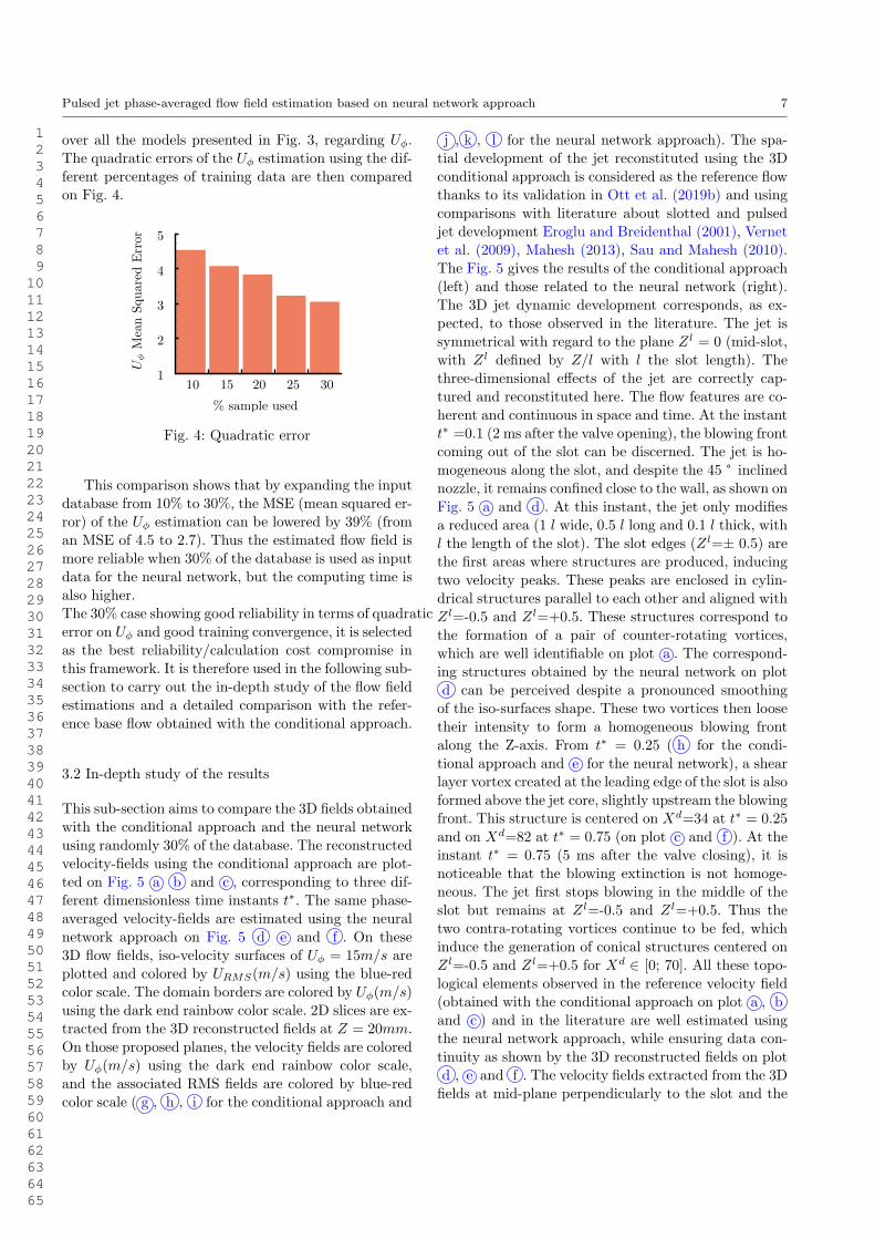
over all the models presented in Fig. 3, regarding Uϕ.
The quadratic errors of the Uϕ estimation using the dif-ferent percentages of training data are then compared
on Fig. 4.
Fig. 4: Quadratic error
This comparison shows that by expanding the input
database from 10% to 30%, the MSE (mean squared er-
ror) of the Uϕ estimation can be lowered by 39% (from
an MSE of 4.5 to 2.7). Thus the estimated flow field is
more reliable when 30% of the database is used as input
data for the neural network, but the computing time is
also higher.
The 30% case showing good reliability in terms of quadratic
error on Uϕ and good training convergence, it is selected
as the best reliability/calculation cost compromise in
this framework. It is therefore used in the following sub-
section to carry out the in-depth study of the flow field
estimations and a detailed comparison with the refer-
ence base flow obtained with the conditional approach.
3.2 In-depth study of the results
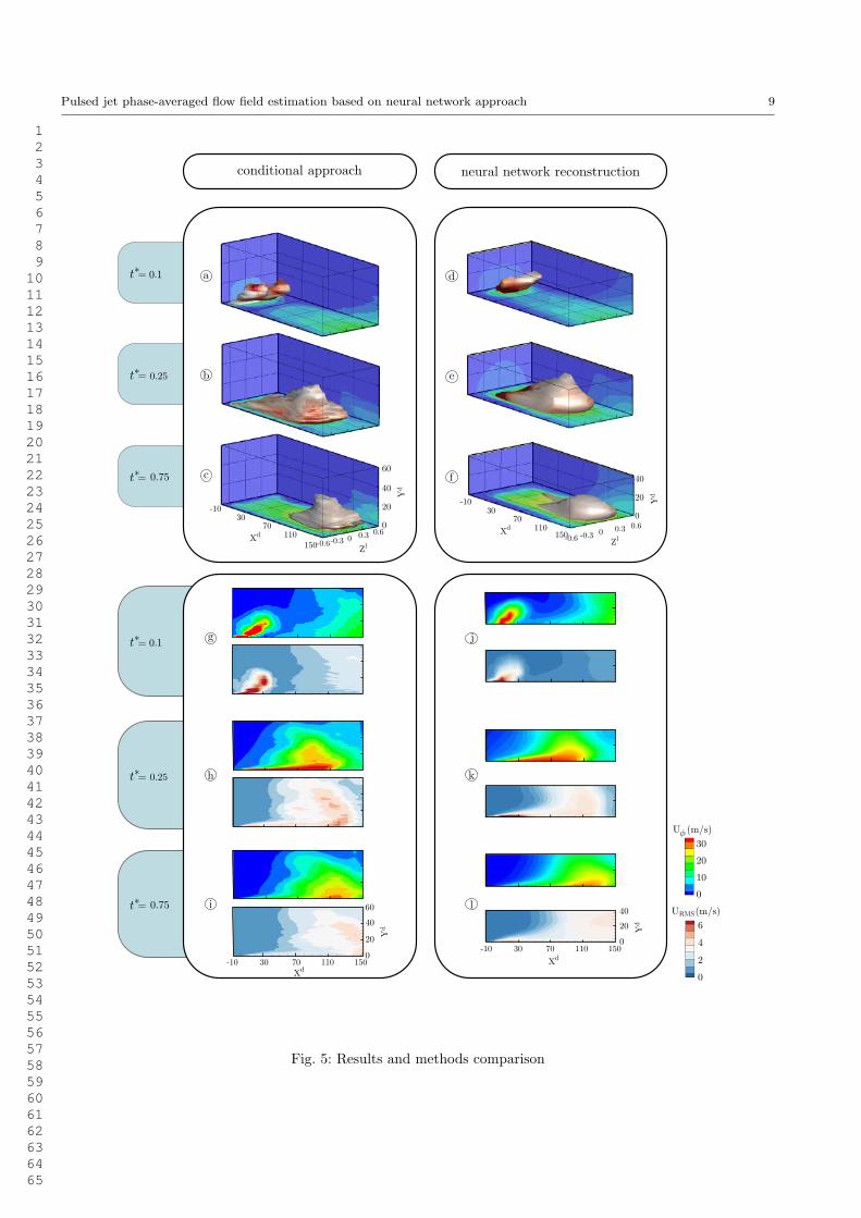
This sub-section aims to compare the 3D fields obtained
with the conditional approach and the neural network
using randomly 30% of the database. The reconstructed
velocity-fields using the conditional approach are plot-
ted on Fig. 5 a b and c , corresponding to three dif-
ferent dimensionless time instants t∗. The same phase-
averaged velocity-fields are estimated using the neural
network approach on Fig. 5 d e and f . On these
3D flow fields, iso-velocity surfaces of Uϕ = 15m/s are
plotted and colored by URMS(m/s) using the blue-red
color scale. The domain borders are colored by Uϕ(m/s)
using the dark end rainbow color scale. 2D slices are ex-
tracted from the 3D reconstructed fields at Z = 20mm.
On those proposed planes, the velocity fields are colored
by Uϕ(m/s) using the dark end rainbow color scale,
and the associated RMS fields are colored by blue-red
color scale ( g , h , i for the conditional approach and
j , k , l for the neural network approach). The spa-
tial development of the jet reconstituted using the 3Dconditional approach is considered as the reference flow
thanks to its validation in Ott et al. (2019b) and using
comparisons with literature about slotted and pulsed
jet development Eroglu and Breidenthal (2001), Vernet
et al. (2009), Mahesh (2013), Sau and Mahesh (2010).
The Fig. 5 gives the results of the conditional approach
(left) and those related to the neural network (right).
The 3D jet dynamic development corresponds, as ex-
pected, to those observed in the literature. The jet is
symmetrical with regard to the plane Zl = 0 (mid-slot,
with Zl defined by Z/l with l the slot length). The
three-dimensional effects of the jet are correctly cap-
tured and reconstituted here. The flow features are co-
herent and continuous in space and time. At the instant
t∗ =0.1 (2 ms after the valve opening), the blowing front
coming out of the slot can be discerned. The jet is ho-
mogeneous along the slot, and despite the 45 ° inclinednozzle, it remains confined close to the wall, as shown on
Fig. 5 a and d . At this instant, the jet only modifies
a reduced area (1 l wide, 0.5 l long and 0.1 l thick, with
l the length of the slot). The slot edges (Zl=± 0.5) are
the first areas where structures are produced, inducing
two velocity peaks. These peaks are enclosed in cylin-
drical structures parallel to each other and aligned with
Zl=-0.5 and Zl=+0.5. These structures correspond to
the formation of a pair of counter-rotating vortices,
which are well identifiable on plot a . The correspond-
ing structures obtained by the neural network on plotd can be perceived despite a pronounced smoothing
of the iso-surfaces shape. These two vortices then loose
their intensity to form a homogeneous blowing front
along the Z-axis. From t∗ = 0.25 ( h for the condi-
tional approach and e for the neural network), a shear
layer vortex created at the leading edge of the slot is also
formed above the jet core, slightly upstream the blowing
front. This structure is centered on Xd=34 at t∗ = 0.25
and on Xd=82 at t∗ = 0.75 (on plot c and f ). At the
instant t∗ = 0.75 (5 ms after the valve closing), it is
noticeable that the blowing extinction is not homoge-
neous. The jet first stops blowing in the middle of the
slot but remains at Zl=-0.5 and Zl=+0.5. Thus the
two contra-rotating vortices continue to be fed, which
induce the generation of conical structures centered on
Zl=-0.5 and Zl=+0.5 for Xd ∈ [0; 70]. All these topo-
logical elements observed in the reference velocity field
(obtained with the conditional approach on plot a , b
and c ) and in the literature are well estimated using
the neural network approach, while ensuring data con-
tinuity as shown by the 3D reconstructed fields on plot
d , e and f . The velocity fields extracted from the 3D
fields at mid-plane perpendicularly to the slot and the
1 2 3 4 5 6 7 8 9 10 11 12 13 14 15 16 17 18 19 20 21 22 23 24 25 26 27 28 29 30 31 32 33 34 35 36 37 38 39 40 41 42 43 44 45 46 47 48 49 50 51 52 53 54 55 56 57 58 59 60 61 62 63 64 65
8 Celetin Ott et al.
wall also show good restitution of the phase-averaged
dynamic response of the actuator inside the jet com-pared to the base flow. Plot g , h and i show that
the jet core (defined by Uϕ ≥ 30 m/s) is 45 ° inclined
at t∗=0.1, with a jet core length of 36d (with d the slot
width). The jet is then confined close to the wall and is
120d long at t∗=0.25 (on h ).
At this time the shear layer vortex is clearly vis-
ible. During the blowing half-period, the average core
velocity is Uϕ =32 m/s, with an average rms velocity of
URMS =7 m/s. At t∗=0.75 ( i ), the actuator is turned
off, and the last flow features are advected (mainly the
jet core and the shear layer vortex). Plot j , k and
l show the flow-fields obtained using the neural net-
work approach. At t∗=0.1 ( j ), the jet core is 45 ° as
expected given the previous results. However, the jet
core is only 0.4L long, and the average rms velocity in-
side the jet core is URMS =5 m/s. At t∗=0.25 ( k ), the
mean and rms velocities fields are smoothed (jet core
is only 1.5L long) and the shear layer vortex is observ-
able but its boundary is not sharply demarcated. The
advection velocity of the main flow features is well mod-
eled (the vortex and jet core are located where they are
expected with regard to the conditional approach). At
t∗=0.75 ( l ) the jet envelop is well estimated despite
a slightly smoothed border. The rms field also show
a globally underestimated intensity without modifying
the shape of the rms field and isolines. Overall the com-
parison of 2D fields allows to highlight that the stan-
dard deviations seem to be globally underestimated by
the neural network: on average by 36% in the jet core,
and by 12% in its surrounding. Moreover, the outline
of the jet core is smoothed and spread out: the jet core
surface and the jet length are underestimated. However,
the mesh of the neural network estimation plot is not
degraded compared to the base flow plot one, which
means that the method allows to obtain the same over-
all phase-averaged flow dynamics as in the base flow by
using only 30% of the experimental data. In order to
quantitatively study the performance of the neural net-
work method, the signals reconstructed by this method
are extracted locally for a phase-averaged period and
overlaid with the phase-averaged hot wire experimen-
tal data. These comparisons are shown in Fig. 6. The
comparison locations are chosen close to the actuator
slot, where the velocity gradient is the highest, and thus
where the velocity estimation in time is more challeng-
ing. These locations are the following: the point 1 is
placed at Xd=2, Y d=1 and Zl=0 (1 mm downstream
the slot and 0.5 mm from the wall). The point 2 is at
Xd=30, Y d=20 and Zl=0 (15 mm downstream the slot
and 10 mm from the wall). Fig. 6 1 and 2 show that
the main dynamic of the signal is well estimated by the
neural network. Indeed, plot 1 shows that the blow-
ing edge reach this location at t∗=0.15 on the referencebase flow (Conditional Approach), and at t∗=0.17 on
the signal given by the neural network, i.e. an error of
13%. The velocity peak occurs at t∗=0.31 for the ref-
erence signal and is anticipated by the neural network
at t∗=0.30 (3% error). On plot 2 , this error is reduced
to 6% for the blowing edge (t∗=0.31 for the reference
signal estimated at t∗=0.29 by the neural network) and
to 2% for the velocity peak (t∗=0.38 for the reference
signal and t∗=0.37 for the neural network).
The dynamics and the average characteristics of the
flow are locally well estimated by the neural network
(the shapes of the curves are identical and the tem-
poral errors remain low). However, the neural network
strongly smooths the velocity variations of low ampli-
tude, filtering out high frequencies.
In terms of amplitude the time-averaged velocity is well
estimated by the neural network, with an underestima-tion of 5% at the location 1 and overestimation of 12%
at the location 2 . However, the velocity peaks are both
underestimated by the neural network in terms of am-
plitude, with an error of 13% at 1 and 4.8% at 2 .
This local comparison confirms the observations made
on 2D and 3D fields: the neural network is able, us-
ing only 30% of the original data, to reliably estimate
the phase-averaged velocity, especially the mean behav-
ior of the velocity. However, the velocity signals are
smoothed (high-frequency features are filtered) and tend
to underestimate the velocity amplitude.
These limitations of the neural network-based method
(underestimated velocity intensity and smoothed out-
line of the jet core) could result from various roots:
◦ the removal of 30% of the database
◦ the neural network architecture
◦ a too small number of trained weights in the neural
network
◦ the choice of the activation function in the neural
network
The method however allows a reliable estimation,
since the main flow features are well estimated in space
and time. The reconstruction by the neural network
is therefore a relevant method for the 3D estimation
of space-time-resolved fields, based on the learning of
experimental data chosen randomly in space and time.
4 Global discussion
This section aims to compare the effectiveness and ca-
pabilities of both methods presented in this paper. Ta-
ble 1 gathers the advantages and limitations found in
1 2 3 4 5 6 7 8 9 10 11 12 13 14 15 16 17 18 19 20 21 22 23 24 25 26 27 28 29 30 31 32 33 34 35 36 37 38 39 40 41 42 43 44 45 46 47 48 49 50 51 52 53 54 55 56 57 58 59 60 61 62 63 64 65
Pulsed jet phase-averaged flow field estimation based on neural network approach 9
Fig. 5: Results and methods comparison
1 2 3 4 5 6 7 8 9 10 11 12 13 14 15 16 17 18 19 20 21 22 23 24 25 26 27 28 29 30 31 32 33 34 35 36 37 38 39 40 41 42 43 44 45 46 47 48 49 50 51 52 53 54 55 56 57 58 59 60 61 62 63 64 65

10 Celetin Ott et al.
Fig. 6: Local estimation in time
the present study regarding the use of the neural net-
work versus the conditional approaches. The conditional
approach is a versatile and quick method that is simple
to implement. The neural network, meanwhile, requires
more time and preliminary studies to be implemented
and validated. Increased attention has to be brought
to the analysis of the results in order to validate the
consistency of the estimated physics. The conditional
approach is quicker than the present neural network
in terms of computational time. The complete process
(from rough data to reconstructed flow fields) is 70
times higher using the neural network than the con-
ditional approach (30 hours versus 25 minutes). The
learning process of the neural network itself is responsi-
ble for 99.5% of the computational time, which means
that once the model is defined the time needed for the
flow field estimation is neglectable. Furthermore, the
conditional approach only provides flow fields with a
coarser or equal resolution (in space and in time) than
the experimental data, while the neural network ap-
proach allows refining both spatial and time-resolutions.
This comes from the fact that the conditional approach
only reconstitutes the flow field based on the experimen-
tal measurements, while the neural network can model
the complete flow field. This study has shown that it is
possible to improve drastically the temporal and spa-
tial resolution of the flow field estimation compared to
the resolution of the measurements, without too much
flow dynamics losses. The main limitation of the present
neural network approach is the processing time, which
led in this paper to a randomized reduction of the learn-
ing database and therefore a deterioration of the estima-
tion. Furthermore, the neural network method showed
smoothed velocity fields and underestimated standard
deviations, which could come from the fact that only
30% of the original data were used, or that the architec-
ture of the neural network was not perfectly suited (too
low number of weights, activation function choice ...). In
order to decrease the computational time of the learn-
ing process while increasing the input database size, it
would be necessary to look to structural optimization
of the neural network and its architecture, as proposed
by Dubois et al. (2020) and Idrissi et al. (2016). In-
deed, a too-small number of trained weights (i.e. not
enough hidden layers/neurons) can lead to smoothed
results, while too many trained weights (i.e. large num-
ber of hidden layers/neurons) can lead to over-fitted
results. Parameter studies can provide a more robust
neural network with better performances (Hamwood
et al. (2018)). In addition, rather than using the classi-
cal sigmoid activation function, the literature suggests
that using more subtle activation function (e.g. relus
functions) could allows to prevent neural network over-
fittings (Ramachandran et al. (2018)).
Such an optimized neural network could open doors
to many interesting applications in the flow field esti-
1 2 3 4 5 6 7 8 9 10 11 12 13 14 15 16 17 18 19 20 21 22 23 24 25 26 27 28 29 30 31 32 33 34 35 36 37 38 39 40 41 42 43 44 45 46 47 48 49 50 51 52 53 54 55 56 57 58 59 60 61 62 63 64 65
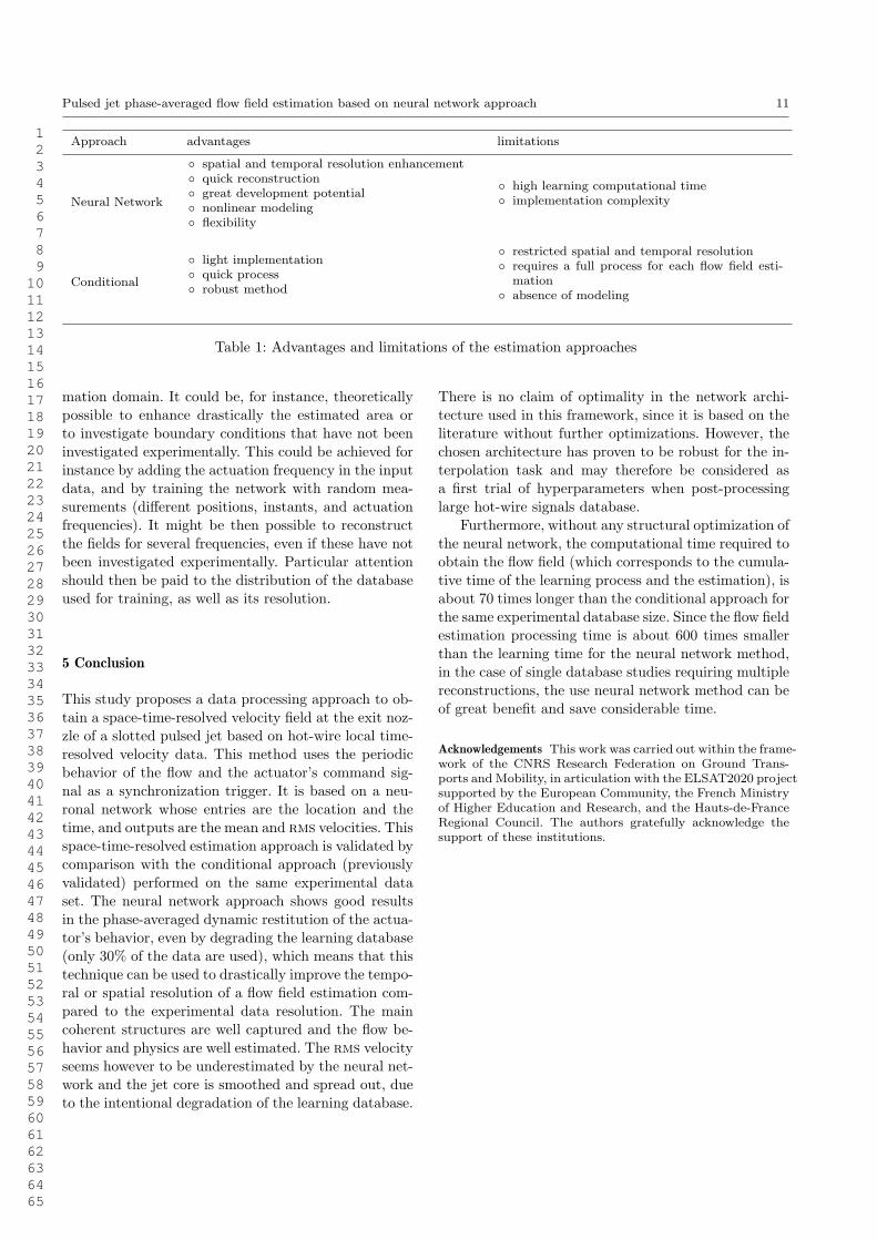
Pulsed jet phase-averaged flow field estimation based on neural network approach 11
Approach advantages limitations
Neural Network
◦ spatial and temporal resolution enhancement◦ quick reconstruction◦ great development potential◦ nonlinear modeling◦ flexibility
◦ high learning computational time◦ implementation complexity
Conditional
◦ light implementation◦ quick process◦ robust method
◦ restricted spatial and temporal resolution◦ requires a full process for each flow field esti-
mation◦ absence of modeling
Table 1: Advantages and limitations of the estimation approaches
mation domain. It could be, for instance, theoretically
possible to enhance drastically the estimated area or
to investigate boundary conditions that have not been
investigated experimentally. This could be achieved for
instance by adding the actuation frequency in the input
data, and by training the network with random mea-
surements (different positions, instants, and actuation
frequencies). It might be then possible to reconstruct
the fields for several frequencies, even if these have not
been investigated experimentally. Particular attention
should then be paid to the distribution of the database
used for training, as well as its resolution.
5 Conclusion
This study proposes a data processing approach to ob-
tain a space-time-resolved velocity field at the exit noz-
zle of a slotted pulsed jet based on hot-wire local time-
resolved velocity data. This method uses the periodic
behavior of the flow and the actuator’s command sig-
nal as a synchronization trigger. It is based on a neu-
ronal network whose entries are the location and the
time, and outputs are the mean and rms velocities. This
space-time-resolved estimation approach is validated by
comparison with the conditional approach (previously
validated) performed on the same experimental data
set. The neural network approach shows good results
in the phase-averaged dynamic restitution of the actua-
tor’s behavior, even by degrading the learning database
(only 30% of the data are used), which means that this
technique can be used to drastically improve the tempo-
ral or spatial resolution of a flow field estimation com-
pared to the experimental data resolution. The main
coherent structures are well captured and the flow be-
havior and physics are well estimated. The rms velocity
seems however to be underestimated by the neural net-
work and the jet core is smoothed and spread out, due
to the intentional degradation of the learning database.
There is no claim of optimality in the network archi-
tecture used in this framework, since it is based on the
literature without further optimizations. However, the
chosen architecture has proven to be robust for the in-
terpolation task and may therefore be considered as
a first trial of hyperparameters when post-processing
large hot-wire signals database.
Furthermore, without any structural optimization of
the neural network, the computational time required to
obtain the flow field (which corresponds to the cumula-
tive time of the learning process and the estimation), is
about 70 times longer than the conditional approach for
the same experimental database size. Since the flow field
estimation processing time is about 600 times smaller
than the learning time for the neural network method,
in the case of single database studies requiring multiple
reconstructions, the use neural network method can be
of great benefit and save considerable time.
Acknowledgements This work was carried out within the frame-work of the CNRS Research Federation on Ground Trans-ports and Mobility, in articulation with the ELSAT2020 projectsupported by the European Community, the French Ministryof Higher Education and Research, and the Hauts-de-FranceRegional Council. The authors gratefully acknowledge thesupport of these institutions.
1 2 3 4 5 6 7 8 9 10 11 12 13 14 15 16 17 18 19 20 21 22 23 24 25 26 27 28 29 30 31 32 33 34 35 36 37 38 39 40 41 42 43 44 45 46 47 48 49 50 51 52 53 54 55 56 57 58 59 60 61 62 63 64 65
12 Celetin Ott et al.
References
Adrian RJ (1979) Conditional eddies in isotropic tur-
bulence. Physics of Fluids 22(11):2065–2070Aeschlimann V, Barre S, Djeridi H (2013) Unsteady
Cavitation Analysis Using Phase Averaging and Con-
ditional Approaches in a 2D Venturi Flow. Open
Journal of Fluid Dynamics 03(03):171–183
Bera JC, Michard M, Grosjean N, Comte-Bellot G
(2001) Flow analysis of two-dimensional pulsed jets
by particle image velocimetry. Experiments in Fluids
31(5):519–532
Bisgaard C (1983) Velocity fields around spheres
and bubbles investigated by laser-doppler anemom-
etry. Journal of Non-Newtonian Fluid Mechanics
12(3):283–302
Bonnet JP, Cole DR, Delville J, Glauser MN, Ukei-
ley LS (1994) Stochastic estimation and proper or-
thogonal decomposition: Complementary techniquesfor identifying structure. Experiments in Fluids
17(5):307–314
Bright I, Lin G, Kutz JN (2013) Compressive sensing
based machine learning strategy for characterizing
the flow around a cylinder with limited pressure mea-
surements. Physics of Fluids 25(12)
Callaham JL, Maeda K, Brunton SL (2019) Robust flow
reconstruction from limited measurements via sparse
representation. Physical Review Fluids 4(10)
Cambonie T, Aider JL (2014) Transition scenario of the
round jet in crossflow topology at low velocity ratios.
Physics of Fluids 26(8)
Cambonie T, Gautier N, Aider JL (2013) Experimen-
tal study of counter-rotating vortex pair trajectories
induced by a round jet in cross-flow at low velocity
ratios. Experiments in Fluids 54(3)
Chovet C, Lippert M, Keirsbulck L, Foucaut JM (2016)
Dynamic characterization of piezoelectric micro-
blowers for separation flow control. Sensors and Ac-
tuators, A: Physical 249:122–130Chovet C, Lippert M, Foucaut JM, Keirsbulck L (2017)
Dynamical aspects of a backward-facing step flow
at large Reynolds numbers. Experiments in Fluids
58(11)
Cole DR, Glausen MN (1998) Applications of stochas-
tic estimation in the axisymmetric sudden expansion.
Physics of Fluids 10(11):2941–2949
Dubois P, Gomez T, Planckaert L, Perret L (2020)
Data-driven predictions of the Lorenz system. Phys-
ica D: Nonlinear Phenomena 408
Emerick TM, Ali MY, Foster CH, Alvi FS, Popkin SH,
Cybyk BZ (2012) SparkJet actuator characterization
in supersonic crossflow. 6th AIAA Flow Control Con-
ference 2012
Eroglu A, Breidenthal RE (2001) Structure, penetra-
tion, and mixing of pulsed jets in crossflow. AIAAjournal 39(3):417–423
Fadla F, Graziani A, Kerherve F, Mathis R, Lippert M,
Uystepruyst D, Keirsbulck L (2016) Electrochemical
Measurements for Real-Time Stochastic Reconstruc-
tion of Large-Scale Dynamics of a Separated Flow.
Journal of Fluids Engineering, Transactions of the
ASME 138(12)
Fernandez P, Delva J, Ott C, Maier P, Gallas Q (2018)
Experimental Measurement Benchmark for Com-
pressible Fluidic Unsteady Jet. Actuators 7(3):58
Foucaut JM, Coudert S, Stanislas M (2009) Unsteady
characteristics of near-wall turbulence using high rep-
etition stereoscopic particle image velocimetry (PIV).
Measurement Science and Technology 20(7)Goodfellow IJ, Shlens J, Szegedy C (2015) Explaining
and Harnessing Adversarial Examples. 3rd Interna-
tional Conference on Learning RepresentationsGuezennec YG, Choi WC (1988) Stochastic estimation
of coherent structures in turbulent boundary layers.
Proceedings of the International Centre for Heat and
Mass Transfer pp 453–468
Haack SJ, Land HB, Cybyk B, Ko HS, Katz J (2008)
Characterization of a high-speed flow control actu-
ator using digital speckle tomography and PIV. 4th
AIAA Flow Control ConferenceHamwood J, Alonso-Caneiro D, Read SA, Vincent SJ,
Collins MJ (2018) Effect of patch size and network
architecture on a convolutional neural network ap-
proach for automatic segmentation of OCT retinal
layers. Biomedical Optics Express 9(7):3049Hardy P, Barricau P, Belinger A, Caruana D, Cam-
bronne JP, Gleyzes C (2010) Plasma synthetic jet for
flow control. 40th AIAA Fluid Dynamics Conference
Hornik K (1991) Approximation capabilities of mul-
tilayer feedforward networks. Neural Networks
4(2):251–257
Hudy LM, Naguib A, Humphreys WM (2006) Stochas-
tic estimation of a separated-flow field using wall-
pressure-array measurements. Collection of Techni-
cal Papers - 44th AIAA Aerospace Sciences Meeting
18:13520–13541
Idrissi MAJ, Ramchoun H, Ghanou Y, Ettaouil M
(2016) Genetic algorithm for neural network architec-
ture optimization. Proceedings of the 3rd IEEE In-
ternational Conference on Logistics Operations Man-
agement, GOL 2016
Jin X, Cheng P, Chen WL, Li H (2018) Prediction
model of velocity field around circular cylinder over
various Reynolds numbers by fusion convolutional
neural networks based on pressure on the cylinder.
Physics of Fluids 30(4)
1 2 3 4 5 6 7 8 9 10 11 12 13 14 15 16 17 18 19 20 21 22 23 24 25 26 27 28 29 30 31 32 33 34 35 36 37 38 39 40 41 42 43 44 45 46 47 48 49 50 51 52 53 54 55 56 57 58 59 60 61 62 63 64 65
Pulsed jet phase-averaged flow field estimation based on neural network approach 13
Jin X, Laima S, Chen WL, Li H (2020) Time-resolved
reconstruction of flow field around a circular cylin-der by recurrent neural networks based on non-time-
resolved particle image velocimetry measurements.
Experiments in Fluids 61(4)
Keras (2018) Guide to the Sequential model - Keras
Documentation
Kotu V, Deshpande B (2019) Deep Learning. Data Sci-
ence 521:307–342
Kovasznay LSG (1949) Hot-wire investigation of the
wake behind cylinders at low Reynolds numbers. Pro-
ceedings of the Royal Society of London Series A
Mathematical and Physical Sciences 198(1053):174–
190
Lakshminarayanan B, Pritzel A, Blundell C (2016) Sim-
ple and Scalable Predictive Uncertainty Estimation
using Deep Ensembles. Cornell UniversityLee S, You D (2019) Data-driven prediction of un-
steady flow over a circular cylinder using deep learn-ing. Journal of Fluid Mechanics 879:217–254
Li Y, Allen-Zhu Z (2019) What can resnet learn effi-
ciently, going beyond kernels? In: 33rd Conference
on Neural Information Processing Systems
Li Y, Chang J, Kong C, Wang Z (2020) Flow field re-
construction and prediction of the supersonic cascade
channel based on a symmetry neural network under
complex and variable conditions. AIP Advances 10(6)Mahesh K (2013) The Interaction of Jets with Cross-
flow. Annual Review of Fluid Mechanics 45(1):379–
407Murray NE, Ukeiley LS (2003) Estimation of the flow-
field from surface pressure measurements in an open
cavity. AIAA Journal 41(5):969–972
Olchewsky F, Desse JM, Donjat D, Champagnat F
(2019) Vertical digital holographic bench for underex-
panded jet gas density reconstruction. Digital Holog-
raphy and 3D Imaging p Th2B.3Ostermann F, Woszidlo R, Nayeri CN, Paschereit
CO (2015) Phase-Averaging Methods for the Nat-
ural Flowfield of a Fluidic Oscillator. AIAA Journal
53(8):2359–2368
Ostermann F, Godbersen P, Woszidlo R, Nayeri CN,
Paschereit CO (2017) Sweeping jet from a flu-
idic oscillator in crossflow. Physical Review Fluids
2(9):2,90512
Ott C (2020) Space-time resolved fluidic actuators char-
acterization, and experimental identification of the
physical mechanisms involved in their interaction
with a boundary layer. PhD Thesis
Ott C, Gallas Q, Delva J, Lippert M, Keirsbulck L
(2019a) High frequency characterization of a sweep-
ing jet actuator. Sensors and Actuators, A: Physical
291:39–47
Ott C, Gallas Q, Delva J, Lippert M, Keirsbulck L
(2019b) Interaction between a jet and a turbulentboundary layer. In: AIAA AVIATION Forum, Dal-
las, USA
Poelma C, Mari JM, Foin N, Tang MX, Krams R, Caro
CG, Weinberg PD, Westerweel J (2011) 3D Flow re-
construction using ultrasound PIV. Experiments in
Fluids 50(4):777–785
Raissi M, Perdikaris P, Karniadakis GE (2019) Physics-
informed neural networks: A deep learning frame-
work for solving forward and inverse problems involv-
ing nonlinear partial differential equations. Journal of
Computational Physics 378:686–707
Ramachandran P, Barret Z, Le QV (2018) Searching
for activation functions. 6th International Conference
on Learning Representations, ICLR 2018 - Workshop
Track Proceedings
Sau R, Mahesh K (2010) Optimization of pulsed jets in
crossflow. Journal of Fluid Mechanics 653:365–390Schaeffler NW, Hepnery TE, Jones GS, Kegerise MA
(2002) Overview of active flow control actuator devel-
opment at NASA Langley research center. 1st Flow
Control Conference
Soria J, Atkinson C (2008) Towards 3C-3D digital holo-
graphic fluid velocity vector field measurement - To-
mographic digital holographic PIV (Tomo-HPIV).
Measurement Science and Technology 19(7)Sun K, Xiao B, Liu D, Wang J (2019) Deep high-
resolution representation learning for human pose es-
timation. In: CVPR CaliforniaSun L, Gao H, Pan S, Wang JX (2020) Surrogate model-
ing for fluid flows based on physics-constrained deep
learning without simulation data. Computer Meth-
ods in Applied Mechanics and Engineering 361
Szegedy C, Zaremba W, Sutskever I, Bruna J, Erhan D,
Goodfellow I, Fergus R (2014) Intriguing properties
of neural networks. 2nd International Conference on
Learning Representations, ICLR 2014 - Conference
Track ProceedingsTuring AM (1950) Computing Machinery and Intelli-
gence. Parsing the Turing Test: Philosophical and
Methodological Issues in the Quest for the Thinking
Computer pp 23–65
Vernet R, Thomas L, David L (2009) Analysis and re-
construction of a pulsed jet in crossflow by multi-
plane snapshot POD. Experiments in Fluids 47
Williams DR, MacMynowski DG (2012) Brief History
of Flow Control. Fundamentals and Applications of
Modern Flow Control pp 1–20
Zaman KB, McKinzie DJ, Rumsey CL (1989) A Nat-
ural Low-Frequency Oscillation of the Flow over an
Airfoil Near Stalling Conditions. Journal of Fluid Me-
chanics 202(403):403–442
1 2 3 4 5 6 7 8 9 10 11 12 13 14 15 16 17 18 19 20 21 22 23 24 25 26 27 28 29 30 31 32 33 34 35 36 37 38 39 40 41 42 43 44 45 46 47 48 49 50 51 52 53 54 55 56 57 58 59 60 61 62 63 64 65
14 Celetin Ott et al.
Appendices
A1. Conditional approach details
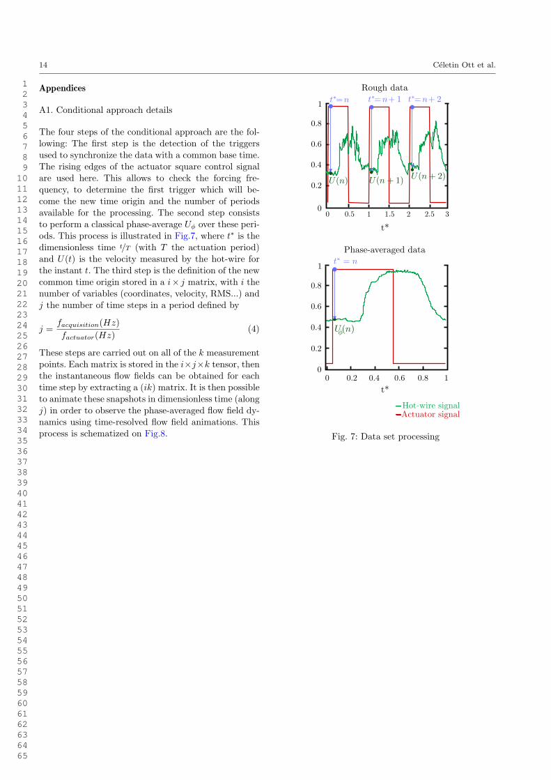
The four steps of the conditional approach are the fol-
lowing: The first step is the detection of the triggers
used to synchronize the data with a common base time.
The rising edges of the actuator square control signal
are used here. This allows to check the forcing fre-
quency, to determine the first trigger which will be-
come the new time origin and the number of periods
available for the processing. The second step consists
to perform a classical phase-average Uϕ over these peri-
ods. This process is illustrated in Fig.7, where t∗ is the
dimensionless time t/T (with T the actuation period)
and U(t) is the velocity measured by the hot-wire for
the instant t. The third step is the definition of the new
common time origin stored in a i× j matrix, with i the
number of variables (coordinates, velocity, RMS...) and
j the number of time steps in a period defined by
j =facquisition(Hz)
factuator(Hz)(4)
These steps are carried out on all of the k measurement
points. Each matrix is stored in the i×j×k tensor, then
the instantaneous flow fields can be obtained for each
time step by extracting a (ik) matrix. It is then possible
to animate these snapshots in dimensionless time (along
j) in order to observe the phase-averaged flow field dy-
namics using time-resolved flow field animations. This
process is schematized on Fig.8. Fig. 7: Data set processing
1 2 3 4 5 6 7 8 9 10 11 12 13 14 15 16 17 18 19 20 21 22 23 24 25 26 27 28 29 30 31 32 33 34 35 36 37 38 39 40 41 42 43 44 45 46 47 48 49 50 51 52 53 54 55 56 57 58 59 60 61 62 63 64 65

Pulsed jet phase-averaged flow field estimation based on neural network approach 15
i
j
k
Fig. 8: 3D-adaped conditional approach Ott et al. (2019b)
1 2 3 4 5 6 7 8 9 10 11 12 13 14 15 16 17 18 19 20 21 22 23 24 25 26 27 28 29 30 31 32 33 34 35 36 37 38 39 40 41 42 43 44 45 46 47 48 49 50 51 52 53 54 55 56 57 58 59 60 61 62 63 64 65

16 Celetin Ott et al.
A2. Neural network: general introduction and terminol-
ogy
In its simplest formulation, a neural network consists
in interconnected units (called neurons) transforming
the input information through a feed-forward process.
One neuron and its associated parameters is shown in
Fig.9. This neuron receives a weighted information Σ =
Fig. 9: Artificial neuron and its associated connections
ω1 × i and activates according to the σ function. Theactivation is classically a sigmoid reading:
σ(Σ) =1
1 + exp(−Σ)(5)
Given a bias b for the neuron and a weight ω2 for the
output, the considered neuron transforms the input i
into o = ω2 × σ(ω1 × i + b). In a dense network, each
connection has a specific weight and each neuron has
a specific bias. The Fig.10 illustrates a simple archi-
tecture: one input layer with one neuron, one hidden
layer with two neurons and one output layer with two
neurons. The input value is x. In the hidden layer, the
upper neuron outputs σ(w1 × x + b1) while the lower
neuron outputs σ(w2 × x+ b2). The neuron in the out-
Fig. 10: Interactions between four neurons
put layer receives a weighted sum of these two outputs
and linearly activates according to:
y = w3 × σ(w1 × x+ b1) + w4 × σ(w2 × x+ b2) (6)
The final output then includes a sigmoid at x = −b1/w1
with an intensity of w3 and another sigmoid at x =
−b2/w2 with an intensity of w4. Just like a linear regres-
sion y = ax+ b would learn the best coefficients a andb from training data points {xi, yi}, a neural network
y = NN(x) learns the optimal weights w and biases b
to recover training examples from sigmoids.
These parameters are learned by minimizing a cost
function which is often the mean square error between
training data and their estimations. Consideringm train-
ing examples, the cost function then reads:
E2 =
m∑t=1
(yt −NNt)2 (7)
Where NNt = NN(xt). The neural network operator
NN is built upon parameters and hyperparameters. Pa-
rameters are optimized via a gradient descent on the
cost function and hyperparameters (number of layers
and number of neurons) are often based on the user
experience.
1 2 3 4 5 6 7 8 9 10 11 12 13 14 15 16 17 18 19 20 21 22 23 24 25 26 27 28 29 30 31 32 33 34 35 36 37 38 39 40 41 42 43 44 45 46 47 48 49 50 51 52 53 54 55 56 57 58 59 60 61 62 63 64 65