pulse power device characterization for amplifier design
TRANSCRIPT

Pulse Power Device Characterization For Amplifier Design.
Paul Fourie.
Thesis submitted in partial fulfillment of the requirements for the degree of Master of Engineering
at the University of Stellenbosch.
Supervisor: Dr. Cornell van Niekerk.
December 2004

Declaration
I, the undersigned, hereby declare that the work contained in this thesis is my own original work,
unless otherwise stated, and has not previously, in its entirety or in part, been submitted at any
university for a degree.
Paul Fourie.

Acknowledgements
Several people contributed to this work in various ways. It would not have been possible without
their help. I would like to thank Dr. Cornell van Niekerk for his help, patience, encouragement and
the fact that he never showed he was “gatvol”.
I would also like to thank Reutech Radar Systems who financially sponsored the first year of the
work.
Further, I would like to thank Wessel Croukamp, Heinz Preuss and Robert Engelbrecht for their
help in building and assembling some of the test setups. A special thanks also to my son Jaco for his
help with the writing of the software that was needed at times.
Most of all I would like to thank Almighty God for making it all possible.

Summary
Keywords: Radar, Class C, power amplifiers, load-pull, pulsed RF, microwave, TRL, MultiMatch,
pulse power, device characterization.
Bi-polar Si transistors optimized for pulse conditions is still the most popular choice as
amplification element in the final stages of solid-state radar amplifiers in L and S band. With the
radar market being small, the design data for these devices is normally fairly limited and it is up to
the designers to thoroughly characterize them for their designs. This is normally done through load-
pull experiments. Professional automated load-pull equipment is very expensive especially at the
higher power levels. In spite of being automated and under computer control, load-pull exercises
still is very time consuming and as such expensive. For small companies that only occasionally need
to design such amplifiers it is not economically viable to acquire such equipment and different
strategies have to be found to stay competitive.
This report investigates such a strategy and its implementation.
A procedure to quickly and accurately characterize such devices was developed and two amplifiers
were designed and build with this procedure and compared to their traditional counterparts for
verification. The results were very promising and with a bit more work, the technique can likely be
used to characterize these devices for design work outside of the parameters designated by the
manufacturers.

Opsomming
Sleutelwoorde: Radar, Klas C, drywings versterkers, lastrek, gepulsde RF, mikrogolf, TRL,
MultiMatch, pulsdrywing, toestel karakterisering.
Bipolere Silikon transistors wat vir werking onder gepulsde toestande geoptimiseer is, is nog steeds
die mees gewilde keuse as versterkingselement in die finale stadiums van vastetoestand radar
versterkers in die L en S bande. Met die radar mark wat geredelik klein is, is die ontwerp inligting vir
hierdie elemente gewoonlik redelik karig en is dit die taak van die ontwerpers om die elemente te
karakteriseer vir hulle ontwerp doeleindes. Dit word normaalweg gedoen deur lastrek eksperimente.
Geoutomatiseerde lastrek toerusting is baie duur, veral as dit onder hoë drywingstoestande moet
werk. Al is die toerusting geoutomatiseer en onder rekenaar beheer, is lastrek oefeninge nog steeds
baie tydrowend en daarom dan ook baie duur. Vir klein maatskappye wat net nou en dan nodig het
om sulke versterkers te ontwerp is dit gewoon nie ekonomies regverdigbaar om sulke toerusting aan
te skaf nie, en ander strategië moet gevind word om ekonomies kompeterend te bly.
Hierdie verslag ondersoek so VWUDWHJLHHQGLHLQSOHPHQWHULQg daarvan.
n Prosedure om gepulsde bipolere transistore vinnig en akkuraat te karakteriseer is ontwikkel en
twee versterkers is met die prosedure ontwerp en gebou. Die versterkers is geverifieer deur hulle
met hulle tradisionele eweknië te vergelyk. Die resultate lyk baie belowend en met n bietjie meer
werk kan die metode waarskynlik ook gebruik word om die transistors buite die toepassings gebied,
soos deur die vervaardigers aangedui, te gebruik.

Table of Contents
1 Introduction ................................................................................................... 1
1.1 Thesis Overview .......................................................................................... 3
1.1.1 Design Considerations......................................................................... 4
1.1.2 Device Modeling ................................................................................. 5
1.1.3 Current Design and Manufacturing Techniques ................................. 6
1.1.4 Device Data Format. ........................................................................... 6
1.1.5 Device Tolerances ............................................................................... 8
1.1.6 Design Techniques to Control Device Parameter Uncertainties ......... 8
1.2 Summary.................................................................................................... 11
2 Test Fixture Design for Device Characterization..................................... 12
2.1 Introduction............................................................................................... 12
2.1.1 Load Pull Techniques........................................................................ 12
2.2 Microstrip TRL Test Fixture ..................................................................... 16
2.2.1 TRL Test Fixture Requirements........................................................ 18
2.2.2 TRL Test Fixture Specification......................................................... 20
2.2.3 TRL Calibration Standard Requirements.......................................... 23
2.3 Stub Tuner for High Standing Wave Ratio Load-Pull Measurements ...... 26
2.3.1 Principle of Operation ....................................................................... 27
2.3.2 Realization......................................................................................... 28
2.4 Impedance Transformation Inserts ........................................................... 30

2.5 DC Biasing ................................................................................................ 31
2.6 Current Sensing Circuitry ......................................................................... 33
2.6.1 Principles of Operation...................................................................... 33
2.7 Time gating circuitry................................................................................. 35
2.8 Conclusion................................................................................................. 38
3 Design and Tuning Procedure for Pulse Power Radar Amplifiers ........ 39
3.1 Introduction............................................................................................... 39
3.2 Large-Signal Transistor Characterization................................................ 39
3.2.1 Radar Specific Large Signal Amplifier Design Considerations........ 40
3.3 Proposed Characterization Method.......................................................... 45
3.3.1 Input impedance characterization...................................................... 45
3.3.2 Output impedance characterization................................................... 53
3.4 Multi Stage Amplifier Design.................................................................... 56
3.5 Summary.................................................................................................... 57
4 Experimental Verification of the Proposed Design Method ................... 58
4.1 Introduction............................................................................................... 58
4.2 TRL Test Fixture Verification ................................................................... 58
4.2.1 Performance Checking ...................................................................... 61
4.3 Stub Tuner Evaluation............................................................................... 64
4.4 Device Characterization, Amplifier Design and Evaluation .................... 65
4.4.1 Characterization of the GHz1014-12. ............................................... 66
4.4.2 Reduced Supply Rail (14V) Characterization of the GHz1014-12... 80
4.4.3 Investigative Comparison for the RZ1214B35Y Device. ................. 82
4.5 Conclusions ............................................................................................... 92

5 Conclusions .................................................................................................. 93
6 References. ................................................................................................... 94
7 Appendix A .................................................................................................. 98
7.1 MATLAB m files. ....................................................................................... 98
7.1.1 TRL ................................................................................................... 98
7.1.2 TRL2 ............................................................................................... 107
7.1.3 TRLstone......................................................................................... 117
8 Appendix B ................................................................................................ 127
8.1 GHz Technology 1014-12 Data Sheet ..................................................... 127
8.2 Philips RZ1214B35Y Data Sheet ............................................................ 129
8.3 MAX881R Data Sheet.............................................................................. 136
9 Appendix C ................................................................................................ 144
9.1 Supportive information............................................................................ 144

1
1 Introduction
The goal of this project is to establish an improved design process for solid state high power
pulsed RF and microwave amplifiers, suited to mainly radar applications at modest cost that
would be affordable for smaller design establishments. The main thrust of the investigation is to
find a way to reliably characterize a spectrum of devices over several sets of operating conditions
in order to choose the most cost effective line-up for the required amplifier and its associated
power supply. The aim is to get round the low frequency instabilities, transition instabilities and
pulse length versus peak power tradeoffs with its associated thermal requirements. Once this is
achieved, it becomes possible to design the required amplifiers within a short time frame with a
high probability to get it right the first time. Cost must also be kept to a minimum.
Solid-state bi-polar power devices for microwave applications became commercially available
during the 1970’s [3,4,6,21,24]. The most severe restriction on the frequency response of solid-
state devices is imposed by the carrier transport time through the different doping regions [8,17].
To work at high frequencies the diffusion lengths has to be as short as possible.
The voltage-current (VI) product however determines the maximum output power of the bipolar
junction transistor (BJT) [2,3,11,29]. The maximum current is restricted by the conducting area
and conductivity, which is a function of the doping of the layers [8,20,25]. Maximum operating
voltage is determined by the Zener breakdown and punch through voltages. However the voltage
breakdown depends not only on the nature of the junction involved but also on the external
circuit arrangement [20,25]. For example, the breakdown voltage for the common-emitter circuit
differs from that of the common base circuit, and the external base impedance influences the
maximum operating voltage before breakdown. With the common-base configuration having the
Chapter

2
higher breakdown voltage it is the preferred topology for the high power bipolar devices in
pulsed mode, in other words for power levels above about 35dBm. Most commercially available
packaged devices have then for this reason the base attached to the case of the package.
A bi-polar transistor is punched through if the space charge region of the collector junction
reaches the emitter junction before avalanche can take place [8]. A high punch through voltage
thus puts a limit on the upper frequency at which the device still has useful gain.
The most common way used by device manufacturers to increase the power capabilities of solid-
state microwave devices is to use several transistors in parallel in the same package. (Single cell
devices are hardly ever used.) Two methods of achieving a multi-cell topology have been
observed:
• Several individual transistors are put down on a very high dielectric constant substrate on
which matching and combining pads has been etched.
• The matching and combining pads are made as part of the wafer. By doing this a single
basic device can be used in several topologies to create devices covering a few power and
frequency bands. However, this means that the associated impedances become very low
and there is a matching/ combining network inside the device package over which the
amplifier designer has no control. This creates serious problems for wideband work or
when an attempt is made to use the device slightly outside of the designated band of
operation.
The market for high power radar devices is small, with the result that device manufacturers
are not keen on spending money on elaborate testing and device characterization
procedures [23]. This is largely left to the end users. (The majority of mass produced high
power microwave devices is intended for the communication bands and these do not
overlap with the designated radar bands.) Normally the device manufacturers provide a
recommended foil pattern for the device with sometimes a few load-pull points included.
3
Examples of these are reproduced in chapter eight appendix B. If this does not fit into the
users mechanical, thermal or power supply constraints; it is up to the user to solve the
problem.
1.1 Thesis Overview
A literature study was performed to determine how this design process was approached in the
past and to determine which routes for future development looked the most promising in the
light that, for modern designs to be successful, the design cycle must be short with very few
iterations to the final product. In addition, upgrades to the product must be easy.
As a starting point, a high power (Thru, Reflect, Line) TRL test fixture has been designed to
accommodate the power load-pull measurements that needed to be made. This test fixture
covered from 200MHz to 3GHz with the frequency band of interest being from 1.2GHz to
1.4GHz [12,13,14,15,16]. In conjunction with this test fixture, stub tuners and “biasing T’s” had
to be designed [18]. A procedure then had to be developed to efficiently characterize devices.
To do the characterization of the input matches a current transformer and resonating circuit was
developed to measure the pulsed collector or drain currents. It was found that this gave a good
indication as to when the input was matched at the frequency point in question without having to
optimize the output power at the same time [22]. The result of this is that the input and output
impedances can be close to independently determined.
Two bipolar devices have been evaluated. The data book foil patterns of the bipolar devices have
been implemented and the power output and other characteristics measured. These devices where
then characterized with the proposed method, and new foil patterns designed with this data and
the output power and other characteristics measured again. The results of the two methods could
then be compared.
A driver amplifier to characterize the devices also had to be designed. This was done using a
GaAs power FET.

4
Lately bipolar microwave power devices with power levels in the region of 500W per device with
medium pulse lengths (~ 150µs at 10% duty cycle) have become available. If one could adjust the
biasing voltage levels, these devices could potentially be used for longer pulse lengths at lower
output powers and/ or duty cycles. This then also creates the possibility of modular designs with
the incorporation of suitable power combiners.
Another new trend is the availability of LDMOS FETs for pulsed microwave applications. These
devices are currently becoming available with power levels in the region of 200W with long pulse
lengths and duty cycles. (>300µs at 10% duty cycle). FETs have the nice feature that it is easy to
match their gates for pulse power conditions [2,3,29]. Normally the low frequency stability
problems can also be taken care of on the gate side of the device [2]. Generally, FETs are also
more tolerant to mismatch conditions than bipolar devices. These characteristics make these
devices very attractive for pulse power work. By using LDMOS FETs as drivers for high power
bipolar devices it should be possible to design very efficient high power pulsed amplifiers.
1.1.1 Design Considerat ions
Tight control of the pulse shape and the associated spectral content are crucial to guarantee the
satisfactory performance of radar amplifiers. A device used in class C operation is non-linear, not
only over the RF cycle, but also over the pulse envelope cycle [8,11]. Stability of the device must
be guaranteed over all these conditions to satisfy the phase and pulse shape requirements of the
amplifier.
The high power levels that radar amplifiers operate at means that heat dissipation becomes a
serious problem. A further complication of this is that as the device heats up during the first
couple of hundreds of nano seconds of the pulse it causes a thermally induced pulse droop, up
to about 1.5dB, depending on the geometry, power rating and package of the device. Depending
on the system parameters it might require sophisticated feedback, biasing and power supply
techniques to counter this effect. High efficiency, adequate heat sinking, proper biasing and

5
maybe even sophisticated feedback techniques are therefore also crucial for the satisfactory
operation of these amplifiers.
For the design of these amplifiers one needs to take more into account than just a set of
impedances to be matched as serious consideration must also be given to efficiency, heat
dissipation and DC bias control to have control over stability and pulse shape.
1.1.2 Devic e Modeling
Heterojunction Bipolar Transistors (HBT) and lateral diffusion metal oxide semiconductor field
effect transistors (LDMOSFET) have become very promising devices for different applications at
microwave and millimeter wave frequencies. However, the mainstay of high power
semiconductor devices for pulsed applications at L, S and C band is still bipolar junction
transistors (BJT).
A useful condition for successful design work is the availability of an accurate large signal model
(LSM) for the device intended to be used for the design. In recent years, several publications in
respectable journals were devoted to the creation of a standard compact model for use in CAD
tools and procedures for the extraction of the parameters needed for use in these models
[1,2,3,7,8,22,26,27,28,32 - 45]. Despite the tremendous work already done on the subject we still
do not have unified, accurate model standards in industry together with the needed automatic
extraction procedures. The reason for this is that the device physics is very complicated, the
range of currents to be modeled is broad, and the power densities at which the devices operate is
very high. All this together with the thermal conductivity restrictions of the semiconductor
materials makes the problem of the creation of a universal LSM for these devices more difficult.
Many of the existing models are based on a solid physical background, but again because of the
difficulties of the problem they end up with many empirical coefficients, that are difficult to
extract. Furthermore, when the model is complicated, an additional difficulty to the extraction
problems is that such a model could show problems with convergence.

6
In the light of the large volume of work done on device modeling, the original tack taken when
this project started was then to design and develop circuitry to do pulsed measurements on the
targeted devices with the intent to do parameter extraction and to use these parameters then in
one of the available CAD tools [1,2,3] to design the intended amplifiers. However, the availability
of the needed test equipment and the previously mentioned difficulties forced the abandonment
of this idea
1.1.3 Current Design and Manufac turing Tec hniques
The majority of microwave power amplifier designs are implemented using microstrip or co-
planar techniques and fin-line at millimeter wave frequencies [2,3,11,24]. The substrates used are
normally from 20mil to 60mil thick with relative dielectric constants ( r) varying from about 2 to
10. The active devices used for amplification are large occupying a fair portion of a wavelength
with connector tabs from 3mm to 15mm wide. The majority of Si bi-polar transistors
manufactured for high power radar applications at L, S and C band, have port impedances with a
UHDOFRPSRQHQWRI RUOHVVZLWKDVLPLODULPDJLQDU\FRPSRQHQW>@
Normally line-transformers are used to impedance match these devices [11]. Usually these lines
KDYH LPSHGDQFHV RI OHVV WKDQ DQG DUH D Tuarter of a wavelength long only when the
impedance to be matched is real, which is hardly ever the case. Hence, the majority of these
matches start with a line transformer that is wider than it is long and have enormous steps in
ZLGWK WR JHW WR WKH OLnes. In the light of this, linear circuit analyzers are useless for the
analysis or synthesis of these matches, the reason being that analytical models for such large step
transitions are still dubious. For this reason electromagnetic simulators are used to analyze these
matches and the synthesis of these matches is still more of an art than a science. Part of the
goals of this thesis is to investigate an alternative approach.
1.1.4 Devic e Dat a Form at .
Very few establishments have the luxury of load-pull equipment for high power measurements.
This means that the only design data available to the designer is that which is supplied by the

7
device manufacturer and this still is the starting point of the majority of radar amplifier designs
[21]. The result can be a costly exercise consisting of several iterations before an acceptable
design is obtained.
• Small Signal Data. For some of the devices specified for continuous wave (CW)
operation the manufacturers supply small signal S-parameters or the S-parameters can be
easily measured. Nevertheless, this is not very useful for power amplifier design. A power
amplifier designed with small signal S-parameters and optimized for gain, usually delivers
from 2dB to 4dB less output power than a properly designed power amplifier [1,2,3,29].
However, techniques have been developed to generate transistor models from the small
signal S-parameters and then use the model to design a power amplifier or oscillator
[1,2,3].
• Matching Foils and Impedance Data. The majority of manufacturers of high power
BJT’s for pulse power applications provide a test foil pattern as the only impedance
design data for their devices. It is difficult to scale these patterns to other substrates if it
cannot be implemented exactly as suggested due to the large impedance steps. A further
complication is that these foil patterns are optimized for a specified supply voltage, pulse
length and duty cycle. Should one need to change any of these parameters, there is no
data available and one can only make an intelligent guess as to what is to be changed and
how. Fortunately, some manufacturers occasionally also provide a few impedance points
as well. This then at least makes it easier for the designer to target an area of the Smith
chart for his impedance matching. With the impedance data it is also quick to determine
if the device is well suited for the intended application by inserting this data into an
amplifier synthesis package such as MultiMatch and establishing the difficulty of
obtaining a suitable match and topology. However it must also be stated that often the
provided impedance data and foil patterns are not very reliable or accurate [21] and hence
the need for device and match characterization.

8
1.1.5 Devic e Toleranc es
Parameter spread within batches. With modern device manufacturing techniques and
automated matching and tuning of the devices the parameter spread within batches can be tightly
controlled with the result that devices from the same batch can be readily exchanged.
Batch to batch parameter spread. For the RZ1214B35Y device from Philips it was observed
that devices from a much older batch than the one from which the device characterization was
done, behave differently in the reference amplifier foil pattern and was even more difficult to
optimize over a broad band than the new device. This is a serious problem if the amplifiers that
are to be designed have to be maintained for a long time as is needed by military equipment.
(Lifespan of more than fifteen years.) Batch to batch device tolerances is hardly ever specified by
manufacturers of these devices. What are normally specified are device tolerances within a batch
implying that one should initially buy enough components from the same batch to also
accommodate the envisaged maintenance needs [6,23].
1.1.6 Design Tec hniques t o Cont rol Devic e Param et er Unc ert aint ies
The MTI ( moving target improvement) factor is a very important design parameter for modern
pulse Doppler radars. This calls for tight control of the following amplifier parameters: pulse
droop, pulse top ripple, in pulse phase variation, pulse to pulse amplitude variation and pulse to
pulse phase stability. All these parameters are influenced to a more or lesser degree by device
characteristic uncertainties. Several methods are used to control the parameter spread and device
uncertainties in an attempt to keep the amplifier performance across a range of temperatures and
conditions within the set tolerances.
• Device combination. An often-used approach is to design balanced amplifiers in an
attempt to control the device tolerances and the input and output interdependencies. This
is even extended to millimeter wave frequencies [29]. An extension of this approach is
implemented by manufacturers such as MA Com and Fujitsu who have some amplifier

9
devices that have two transistors on the same carrier and is intended for a push-pull
application. (See Figure 1. An example of a device intended for a push-pull design.) This
technique desensitizes the amplifier from external impedance changes that can affect the
pulse shape, efficiency and stability. It also provides some averaging of the performance
parameters.
Figure 1. An example of a device intended for a push-pull design.
• Amplifier Combination. An extension of the previous technique is the combination of
amplifiers. Yet this is easier said than done, as the design of high power combiners is a
tricky affair.
When co-planar and microstrip structures are used, binary planar combination structures
is the preferred method of power combining. The main advantage of these structures is
that they provide excellent isolation between amplifiers and can be made with very little
loss if care is taken with the choice of topology and materials used. A further advantage
of these structures is that heat dissipation is easy to control and optimize with these
structures. For in phase power combination at moderate power levels, the Wilkinson
combiner is most commonly used, as this structure is easy to design and implement if
moderate insertion loss can be tolerated. A fair contribution to the insertion loss in a
Wilkinson combiner is caused by the displacement current through the balance resistor.
This loss can be reduced if the Wilkinson combiner is modified to become a Geysel

10
combiner at the expense of a bit more real estate that is needed. At high power levels,
external dump-loads are preferred with the result that branch line and rat race couplers
become the preferred topologies for power combination provided one can tolerate the
extra real estate needed. A further advantage of these couplers are that uneven splits are
fairly simple to implement giving one the freedom of any number of amplifiers that can
be combined with good isolation.
Another approach that is sometimes used is to use non-isolated power combiners with
isolators on all the amplifier outputs. This approach works well if cavity radial combiners
are used in conjunction with long amplifier chains with lots of gain. (The popularity of
this approach is due to the mismatch characteristics of the cavity combiners and the
ample volume that is created by this geometry for the thermal management of the
amplifiers.) However if planar non isolated combiners are used this is a potential recipe
for disaster due to the phase sensitivity of this type of structure and the practical
uncertainties that come with isolators on the amplifier outputs as situations can occur
where the power of more than one amplifier have to be dumped in the dump-load of a
single isolator. Depending on the potential failure mode of the dump-load, a potential
catastrophic chain reaction can occur.
Another popular way to combine amplifiers for large systems is spatial combination
where every radiator in a large antenna array is driven by its own amplifier. This is only
practical for large systems since combining efficiency stays constant. For small systems,
circuit combiners have superior performance at much lower cost.
Sophisticated feedback and power supplies. The thermal characteristics of the device are a
function of the package and mounting construction [8]. The designer has no control over this. In
instances where the thermal droop exceeds the pulse shape specification the pulse shape has to
be controlled by the power supply circuitry with the aid of a feedback loop. In cases like this and
where very short pulses are needed it is crucially important to choose an amplifier topology that
is control friendly [2,3], otherwise, the cost to develop the power-supply could well exceed that of

11
the amplifier. A control friendly topology is one where there is very little inductance between the
capacitor bank on the collector of the device and the device tab as well as very little inductance
between the emitter tab and ground for a bipolar device that is used in common base
configuration. The amount of inductance that can be tolerated would be dictated by the
operational power level of the intended device, its chosen supply rail voltage and the rise and fall
times of the intended pulse. For a 200W device driven from a 40V supply rail one would need to
supply in the order of 12A within the rise time of the intended pulse. For this to happen in less
than 50ns is not uncommon. To find such a control friendly topology and guarantee good
efficiency and impedance matching is a difficult and non-trivial exercise and an amplifier
synthesis package such as MultiMatch is an invaluable tool to aid this process [1].
1.2 Summary
Design techniques for solid-state bipolar radar amplifiers have stayed the same for the last twenty
years. The majority of attempts at improvement are concerned with better and cheaper device
characterization methods [11,21]. LDMOS FETs have recently matured to the point where they
have become serious contenders for inclusion in the driver stages of pulse power amplifiers. A lot
of effort is going into the non-linear modeling of these devices and it is likely the route that will
be followed in future regarding these devices [1,3]. However, for high power applications with
stringent thermal constraints, BJTs are still the preferred design technology [21] and a design
process for their use is presented in chapter three.

12
2 Test Fixture Design for Device Characterizat ion
2.1 Int roduc t ion
Load-pull data has been the mainstay for microwave and RF power amplifier design for many
years. It essentially converts an intractable nonlinear problem into one that can be attacked and
solved using linear techniques and even linear simulators [1]. It gives the designer a simple target
area on the Smith chart on which to base the design of the impedance matching networks. With
the recent availability of good, fast, nonlinear simulators and improving large signal models, it
could be argued that load-pull equipment may go down the road to oblivion. This however is not
evident yet; especially for BJTs.
2.1.1 Load Pull Tec hniques
A power sweep measurement on an active amplification device will indicate that there is some
kind of functional relationship between output power and output match. From this it follows
logically that more than two data points should be measured. Such a measurement is termed a
load-pull measurement. The results of these measurements are normally plotted as contours of
constant power on a Smith chart.
In its simplest form, a load-pull test setup consists of the device under test (DUT) with some
form of calibrated tuning devices on its input and output. The input is normally only adjusted to
optimize gain. However, bipolar transistors show significant dependency between output power
and input load. This complicates load-pull measurements on bipolar transistors, as both input and
output loading have to be adjusted simultaneously.
Chapter

13
Figure 2. Typical Load-pull data.
A typical set of load-pull data is shown in Figure 2. Such a set of data may take weeks, days or
minutes to compile, depending on the degree of complexity, expense, and time invested in the
load-pull measurement equipment. The results show closed contours, marking the boundaries of
specified output power levels. For most practical purposes, the power amplifier designer is
concerned mainly with the –1dB and –2dB contours, which represent levels relative to the
maximum or optimum power output of the device at the test frequency.
The most obvious immediate observation in looking at the data in Figure 2 is that the constant
power contours are not circular, unlike noise and linear mismatch (gain) circles. The reason for
this is that they physically are areas of intersection between constant resistance and constant
conductance circles [3]. This result can be verified by studying the concept of a load line match
and idealizing it [1,2,3].

14
Figure 3. Typical commercial load-pull configuration.
• Commercial Load-Pull Equipment. Most commercially available load-pull test setups
use some form of computer controlled tuning device. A typical block diagram is shown in
Figure 3. Such a system would likely rely on off-line calibration, whereby the impedances
of literally thousands of tuner settings are measured with a calibrated network analyzer
and stored. Mechanical tuners have to be accurately resetable, which presents some design
challenges. They typically are controlled by stepping motors, which introduce additional
mechanical tolerance problems and put some substantial time limits on each
measurement. A further complication of mechanical tuners is their inherent loss. With the
low port impedances of power devices, a loss of fractions of a decibel could potentially
mask the impedance that one is trying to measure. (The loss can be represented by a small
resistance comparable to the real part of the impedance that one is trying to measure.) An
alternative technique is to use so called active tuning. With this technique a test signal is
applied to the output of the device and tuning effects are simulated by varying the phase
and amplitude of the applied signal. This technique however is normally used at very high
frequencies where the design of mechanical tuners becomes extremely difficult [3].

15
At this juncture, it is assumed that the matching problem is essentially a linear one and that the
output current waveform that drives the tuner is perfectly sinusoidal. This is hardly ever the case
as amplifiers designed to work in class C is normally driven at least one decibel into compression.
Devices used in class C are highly non linear, not only over the RF cycle, but also over the pulse
envelope cycle. This raises some complex issues regarding the predictability and repeatability of
the tuner at harmonic frequencies. However, at least in principle, tuners can be calibrated at
harmonic frequencies as well.
2 . 1 . 1 . 1 D E T E R M I N A T I O N O F P O R T I M P E D A N C E S
The optimum impedance to be matched is normally acquired through some variation of a load-
pull experiment [2,3,11,18,21,24,29,30,31]. To get to this “optimum” impedance, load-pulling can
take all the parameters deemed crucial, such as output power and efficiency, into account and
normally an attempt is made to get as close as possible to the conditions of the intended
application. Having said this, it must still be remembered that this “optimum” impedance is
specified with the following understanding:
• The real device is highly non linear, not only over the RF cycle, but also over the pulse
envelope cycle [8,11]. Furthermore, just defining the impedance becomes difficult, to say
nothing of measuring it.
• If it were possible to measure the port impedances under power conditions by applying a
high level of RF power to the device and looking at the reflected signals, those
impedances would be a complex function of the power and it would be quite different
from the conjugate of the optimum input impedance and load under small signal
conditions [2,3,7,11,22,26,27,2830,31]. Some kinds of RF devices, particularly bipolar
transistors, show significant dependency between output power and input load. It is, in
practice, quite difficult to differentiate between true source-pull effects and simple input
matching. Devices that show the most prominent source-pulling effects usually operate
close to their maximum usable frequency, and this situation is best avoided by using a

16
higher frequency technology [3]. Most often, however, devices for pulse power work are
optimized to work close to their maximum usable frequency with the result of a strong
dependency between input and output.
Commercially available load-pull equipment is very expensive. If ones business necessitates the
design of pulse power microwave amplifiers only occasionally, the expense of such equipment
cannot be justified. A test fixture was designed in an attempt to provide a more affordable
solution. Such a test fixture would have to include the means to represent the intended
application closely and characterize the device under test (DUT) accurately.
2.2 Mic rost rip TRL Test Fix ture
The backbone of this test fixture is a microstrip TRL (Thru-Reflect-Line) structure into which
the required measurement modules fits, namely:
• Active device mounting inserts.
• High current biasing inserts.
• Current sensing and gating circuitry.
• Impedance transformation inserts.
• Stub tuner inserts.
The design of each of these inserts will be treated in detail. The basic fixture is shown in Figure 4.

17
Figure 4. Basic Test Fixture.

18
2.2.1 TRL Test Fix t ure Requirem ent s
• Microwave power and direct current (DC) constraints.
The DC and microwave power design parameters for the test fixture is as follows; be able to
accommodate pulse power solid state devices up to 750W peak power with a duty cycle of
10% and a maximum pulse length of 350µs. The DC supply for these devices would normally
be between 40V and 60V but for some of the lower power devices (50 dBm and less) it can
be as low as 10V. This implies that it must be able to safely handle peak currents of 40A.
Since the RF input and output lines can also carry the DC supply current they must be of
adequate dimensions with enough copper area. The copper area needed can be estimated
from the empirically determined formula [9];
I = 0.048 T0.44 A0.725 (1)
Where the units are
I Ampere
T Temperature Rise in °C
A Cross sectional area in square mils (square THOU)
Since pulsed conditions places greater stress on substrates than DC conditions [9] one will do
well to be conservative. With this formula a 9mm wide 2oz/ feet2 copper track can carry
25.8A average current with a 20°C rise in temperature. This should be adequate for the
maximum-pulsed current conditions envisaged [9]. (Forty amps peak with a low duty cycle.)
Due to the relatively high power levels and the potentially high voltage standing wave ratio
(VSWR) that could exist on the lines, N-type launchers where chosen to be on the safe side.

19
• Mechanical considerations.
The first requirement of the TRL calibration approach is the ability to insert and replace
calibration standards of different physical dimensions with ease. Closely linked to this
requirement is the ability to insert and remove the devices to be tested with ease after the
measurement planes have been fixed at the end of the transmission lines through calibration.
As both the calibration standards and devices to be measured have to fit between two
transmission lines, a so-called split-block design is normally used for TRL test fixtures. Good
guidelines on the mechanical design of TRL fixtures can be found in reference . [10].
Connection repeatability and a stable measurement environment are crucial parameters for
any calibration procedure. Therefore one should also try to keep the feed lines about the
same width as the DUT tabs as substantial differences in width can lead to numerous
measurement and repeatability problems [11,21]. The devices to be measured have tab widths
that vary from about 3mm wide to about 15mm wide. With this in mind, a test fixture with
microstrip lines of about 9mm wide would be a good choice.
For accurate error correction, the system must be stable and the connection interface
repeatable. The radiated electric fields around the microstrip lines in the fixture may change
somewhat between calibration and measurement (due to the changes in grounding and
transmission line alignment caused by the fixture separation during calibration and device
measurement). Most of the microwave signal propagates through the dielectric between the
surface conductor and the ground plane below the dielectric.
Figure 5. Microstrip transmission line geometry and electric fields.

20
However, as shown in Figure 5, some of the signal is supported by electric fields in the air above
the substrate. As objects are introduced into the electric fields above the surface or when the
fixture is separated, the propagation characteristics of the microstrip transmission line will
change. To minimize this effect, the test environment should be repeatably the same during
calibration and measurement. Further, the test environment should be similar to that of the final
application. In practice, this means that the ends of the mating blocks must be machined very flat
and measures must be taken to get their heights exactly the same as to keep the discontinuity in
the transmission medium to a minimum. Measures must also be taken to minimize the
disturbance (discontinuity) of the electrical connection between transmission lines while
maintaining good and repeatable electrical contact.
2.2.2 TRL Test Fix t ure Spec if ic at ion.
From the discussed requirements, a specification for the basic TRL test fixture can be extracted.
The guide specification is as follows:
• Preferred connectors. N-type (female).
• Current handling capability. 40A peak. (350µs pulse, 10% duty cycle).
• Ideal microstrip width. ~ 9mm.
• Ideal channel width containing the microstrip lines. <20mm.
• Preferred physical length of guiding structure. ~ 500mm.
• Simplicity in exchanging calibration standards and devices to be characterized.
• Measurement repeatability. Better than 30dB.

21
2 . 2 . 2 . 1 C H O I C E O F S U B S T R A T E
The diameter of the dielectric material of a N-type connector is close to 9mm. When an N-type
connector is used as launcher onto microstrip, the ideal height for the microstrip dielectric
material would be about 4.5mm to minimize the step in ground conductor.
With these requirements and restrictions in mind, Aluminium backed 125 mil (3.2mm) Arlon
5278 with 2 oz/ ft2 copper, which was left over from another project was chosen as substrate for
WKH75/WHVWIL[WXUH7KLVVXEVWUDWHKDVDUHODWLYHGLHOHFWULFFRQVWDQW r) of 2.6, which means 50
Ω microstrip-lines are 8.85mm wide. The effective dielectric constant for this line is 2.2 and a
wavelength at L-band is then about 200mm. This proved to be an adequate choice.
2 . 2 . 2 . 2 M E A S U R E M E N T R E P E A T A B I L I T Y
Good stable electrical connection between transmission conductors and the continuity of the
ground plane is of vital importance for good measurement repeatability. The ground continuity is
ensured by machining the mating surfaces very flat and by maintaining tight tolerances
throughout the manufacturing of the test fixture.
Electrical connection between microstrip transmission lines is provided by a thin piece of
conductor (0.2mm thick brass shim) on the end of a dielectric block bridging the conductors, as
shown in Figure 6. Low loss machinable foam with a dielectric constant of 1.09 and dissipation
factor of 0.0004 from the Cuming Microwave Corporation (RH-5) was found to work well as
dielectric blocks.

22
Support
Dielectric Block
Shim
Substrate
Track
Backing
Figure 6. Line connecting detail.
While making the connection, the dielectric block and brass shim will disturb the fields above the
surface. The impedance of the line is partially dependent on the total thickness of the surface
conductor. As the bridging conductor is pressed into place, there is unavoidably a small
impedance discontinuity. Therefore, the dimensions of the shim and dielectric block should be
kept to a practical minimum. (Bigger connections need bigger shims with wider blocks). The
alignment of the shim was found to be a critical factor for good measurement repeatability. It
was found that the shim must be exactly the same width as the narrowest line and it must line up
squarely on both sides. A slight step in height between the two lines to be connected was found
to have an even bigger influence on measurement repeatability than a slight miss-alignment in the
connecting shims. For this reason the flatness of the components of the measurement fixture
must be well maintained. With care and practice, a measurement repeatability of better than 40dB
can be achieved. A step in height of about 0.1mm will drop this figure to less than 20dB and a
miss-alignment of about 0.5mm on 10mm wide lines will drop this figure to about 30dB.

23
2.2.3 TRL Calibrat ion St andard Requirem ent s
When building a set of standards for a user-defined environment, the requirements for each of
these standard types must be satisfied. An important note here is that TRL does not require a
perfect short or open, just that the source of the reflection at the two measurement planes are
identical and that the characteristic impedance of the through and line standards are the same.
Requirements for TRL standards
Standard Requirements
Reflect 5HIOHFWLRQFRHIILFLHQW PDJQLWXGHRSWLPDOO\QHHGQRWEHNQRZQ3KDVHRI PXVWEHNQRZQZLWKLQZDYHOHQJWK0XVWEH WKH VDPH RQERWKSRUWs.
May be used to set the reference plane if the phase response of the REFLECT is
well known.
Zero Length
Thru
S21 and S12 are defined equal to 1 at 0 degrees (typically used to set the reference
plane). S11 and S22 is defined equal to zero.
N on-Zero
Length
THRU
Characteristic impedance Z0 of the THRU and LINE must be the same.
Attenuation of the THRU need not be known. Insertion phase or electrical length
must be specified if the THRU is used to set the reference plane.
LIN E
Z0 of the LINE establishes the reference impedance after error correction is
applied. Insertion phase of the LINE must never be the same as that of the
THRU (zero or non-zero length). Optimal LINE length is 1/ 4 wavelength or 90
degrees relative to the THRU at the center frequency. Useable bandwidth of a
single THRU/ LINE pair is 8:1 (frequency span/ start frequency). Multiple
THRU/ LINE pairs (Z0 assumed identical) can be used to extend the bandwidth
to the extent that transmission lines are realizable. (They might become
impractically short.) Attenuation of the LINE need not be known. Insertion
phase or electrical length need only be specified within 1/ 4 wavelength.

24
2 . 2 . 3 . 1 T R L S T A N D A R D D E S I G N .
• Reflect standard. The simplest REFLECT would be an open circuit. This can be
achieved by simply separating the two TRL test fixture halves. A short circuit could also
be used. With the relatively wide transmission lines that were used it was found that an
open circuit radiate quite a bit of energy. The preferred reflect standard for this project
was therefore a short circuit.
• Thru and Line standards. The LINE standard is a short microstrip line inserted
between the fixture halves. Complete microstrip models indicate that physical length and
electrical length are related by not only the dielectric constant, but also the thickness of
the dielectric, and the dimensions and conductivity of the surface and ground conductors
[20]. However, precise specification of the electrical length is not required in TRL,
particularly when a zero-length THRU is used to set the reference plane. A quasi-TEM
method can be applied to estimate the electrical length. Quasi-TEM infers that the
propagation velocity is essentially constant (non-dispersive) but offset by the effective
dielectric constant [17].
This effective dielectric constant is a function of the line’s dimensions and material. The
recommended electrical length for a LINE standard is between 20 and 160 degrees with
respect to the THRU [10]. In order to cover a greater than 1:8 frequency span, multiple
lines must be used. If the frequency span is less than 1:64, then two THRU/ LINE pairs
will be sufficient. The desired frequency span must be divided, allowing one LINE
standard to be used over the lower portion of the frequency span and a second to be used
for the upper band. The optimal break frequency is the geometric mean frequency
( ).f1 f2 of the total frequency band that needs to be covered. The geometric mean of
0.2 GHz and 3GHz is about 0.8GHz. The optimal line lengths to cover the whole band
would thus be about 26mm and 100mm.

25
A compromise was made and the two line lengths were chosen as 60mm and 30mm for
the lower and upper bands with a zero length THRU. Relative to a zero length THRU, a
60mm line at 0.2GHz is about 22 degrees long and at 1.5GHz, it is about 160 degrees
long. The 30mm line is about 27 degrees long at 0.5GHz and at 3GHz; it is about 160
degrees long. This fixture can thus potentially be used between 200MHz and 3GHz,
provided that no unwanted modes are generated.
2 . 2 . 3 . 2 D E V I C E M O U N T I N G I N S E R T S
The active devices to be tested are mounted on carrier blocks that can then be easily inserted and
extracted from the test fixture. For every different device, or at least for every different package
that are used for device packaging, a carrier block have to be designed and made. Once the active
device is mounted on the carrier block, it can be characterized in the test fixture with repeatability
and ease. An example of such a carrier block is shown in Figure 7. The other passive structures
that might also be needed for the device characterization was mounted on similar blocks, like the
quarter wave transformers that can also be seen in Figure 7.
Figure 7. Carrier block detail.

26
2.3 Stub Tuner for High Standing Wave Rat io Load-Pull Measurements
The design criteria for the tuner is: Be capable to synthesize SWR’s of more than a 100 (R0 <
0.5Ω LQ D V\VWHP KDYH D ° target tuning area on the Smith chart and have a 750W
pulsed power-handling capability.
The key requirement for power load-pull is accurate, very low impedance synthesis at high RF
power levels. Computer controlled electromechanical slide screw tuners have been the designated
state-of-the-art solution for some time [18]. Good electromechanical slide screw tuners can
accurately generate a SWR of the order of 15:1, which corresponds to the real part of the
internal impedance of the transistor to EHPHDVXUHG RI DERXW LQ D V\VWHP 7KLVFRUUHVSRQGV WR D UHIOHFWLRQ FRHIILFLHQW %H\RQG WKLV UHIOHFWLRQ FRHIILFLHQW OHYHO WKHcalibration and repeatability of these tuners may cause accuracy and measurement repeatability
problems [18]. The main restriction of these tuners is insertion loss. A small insertion loss can
mask the low impedance that one is trying to measure. For reflection coefficients very close to
one, this problem is normally solved by the use of quarter wave transformers in conjunction with
the slide screw tuners or by the use of active tuners. The use of quarter wave transformers limits
one to a small tuning area of the Smith chart [18], which can be a serious restriction. Active
tuners are normally only used for low noise (low power) applications, as they are notorious for
their instability and oscillation problems.
Another approach proposed by Focus Microwaves is to transform the very low impedance to be
measured, in two steps, using stub tuners, to get to the needed 5 LPSHGDQFH OHYHO >@7KLVapproach makes a 360° target tuning area on the Smith chart possible with potentially a very low
insertion loss. If the insertion loss and the reactance of the stubs can be kept low enough, such a
structure can potentially be used for the task at hand. Manually tuned stub tuners can be made at
moderate cost with relative ease and this approach was taken. (Sliding line tuners are complex and
difficult to manufacture, with the associated cost penalty).

27
2.3.1 Princ iple of Operat ion
An equivalent circuit model of a two-stub tuner is shown in Figure 8. The majority of power
transistors normally require a large capacitor directly on the collector or drain terminal [11]. For
this reason transmission line TL1 in Figure 8 should be kept as short as is practically possible and
the series inductance in the stubs should be minimized so that C1 can represent this capacitance.
Further one would strive to get the sum of the electrical lengths of TL1 and TL2 to be close to
90° at the center of the frequency band of interest (1.3GHz). This will allow the inverse
impedance of C2 and L2 to be placed at port 1. Both inductive and capacitive loads can thus be
created. (A 360° tuning area on the Smith chart.)
CAP
C=ID=
c pFC1
IND
L=ID=
L nHL1
CAP
C=ID=
c pFC2
IND
L=ID=
L nHL2
TLIN
F0=EL=Z0=ID=
1.3 GHza1 Deg50 OhmTL1
TLIN
F0=EL=Z0=ID=
1.3 GHza2 Deg50 OhmTL2
TLIN
F0=EL=Z0=ID=
1.3 GHza3 Deg50 OhmTL3
PORT
Z=P=x Ohm1
PORT
Z=P=50 Ohm2
inputDUT
Figure 8. Equivalent circuit model of a two-stub tuner.
Another way to view the operation of the tuner is as follows: C1 and L1 generates a reflection
vector that is added to the reflection vector generated by C2 and L2 with the phase addition of
TL2 included. This combination generates a total reflection factor that reaches one at the
reference plane of C1 and L1 [18]. The insertion loss of transmission lines TL1 and TL2
degenerates this reflection factor and places a limit on the minimum impedance that can be

28
characterized. The reflection factor that can be generated is also restricted by the series LC
resonators of the two tuning stubs. Ideally, one would like a pure limitless capacitance that can
vary from zero to infinity. In practice, this capacitor is restricted by the physical dimensions of
the electrical conductors of the transmission medium and by the limits of the separation distance
of the conductors forming the capacitor. The inductors should ideally be zero and one should
take care with their physical construction as their value proved to be the major restriction limiting
the performance of the constructed tuner.
2.3.2 Realizat ion
Stripline was used as the transmission medium. To keep impedance discontinuities to a minimum
the 50Ω stripline conductors need to be close to the same width as the microstrip conductors of
the TRL test fixture, preferably about 0.2mm narrower to ease the mechanical line up procedure
and improve the repeatability of the connection [11]. Height wise the ends of the stripline
conductors must lie flat on the microstrip conductors of the TRL test fixture with about a 1mm
overlap. To minimize loss 0.5mm thick Copper was chosen as the conductor material and low
loss machinable foam with a dielectric constant of 1.09 and dissipation factor of 0.0004 from the
Cuming Microwave Corporation (RH-5) was chosen to support the conductor in the cavity.
The tuning stubs were realized by modifying the moveable parts of moderately priced
micrometers and mounting them in the roof of the structure. This construction can be seen in
Figure 9. The ends of the micrometer measuring rods were covered with thin sheets (0.02mm) of
mica to electrically isolate them from the stripline conductors at very small spacing. The 8mm
diameter of the measurement rods of the micrometers, meant that the maximum capacitor value
that could be realized is about 38pF, translating to a reactance of about 3Ω at 1.3GHz, putting a
restriction on the maximum reflection coefficient that can be generated. (The minimum
capacitance is a couple of tens of femto farad.) Ideally, one would like the inductance
represented by the piece of measurement rod to be zero. In practice, the distance to the
grounding point in the structure and the maximum distance from the line limit this. Originally it
was assumed that the capacitive coupling where the rod came through the roof would be an

29
adequate grounding point, but this proved not to be the case and the amount of series
inductance in the stubs of the original design made the tuner practically unusable. Mounting
grounding fingers in the roof of the structure solved the problem and this improved matters to
the point where a reactance down to less than 3.5Ω could be measured.
Figure 9. Realization of two-stub tuner.
The ideal situation would be for the tuning stubs to sit very close to the measurement planes. In
practice, this distance is limited to more than 30mm, the distance chosen, by the support

30
structures of the test fixture. The spacing between the two tuning stubs were chosen to be about
35mm as space had to be provided for the mounting of the grounding fingers while the
condition of 90° from measurement plane to tuning stub also had to be satisfied. This was found
to be an acceptable approximation of the requirements discussed in the section dealing with the
operational principals.
2.4 Impedance Transformat ion Inserts
The most widely used method of broadband impedance matching between two real impedances
is the quarter wavelength multisection impedance transformer. The design of these transformers
is treated in detail in several textbooks and will not be repeated here [19,20].
Traditionally quarter wave transformers are used to transform the low impedances of microwave
power transistors to an intermediate impedance level around which the load pull tuners that are
available can tune. However, this type of solution presents three major inconveniences: limited
bandwidth of less than 10%, a fixed tuning direction (typically, but not always, 180°) and a fixed
transforming ratio [18]. For every new transistor and frequency range of interest a new set of
transformers have to be designed manufactured and characterized. Fortunately, these
transformers are flexible and fairly low cost and easy to implement, making their inclusion quite
feasible when needed. Single step transformers of this kind were also designed and made for this
project but later found not to be really necessary. However, with the load pull tuners in their
present state, if devices with impedance levels below about 3.5Ω have to be characterized, such
transformers will have to be used. An example of the use of quarter wave transformers can be
seen in Figure 10.

31
Figure 10.Device under test with quarter wavelength transformers.
2.5 DC Biasing
Just as the tracks of the TRL test fixture must be capable of handling 40A peak currents, the
inserts used for DC biasing (bias T’s) must also be capable of this and were therefore chosen to
have the same track widths as the TRL lines. The DC biasing inserts must isolate the DC and
microwave circuitry. In concept, using an inductor with a reactance much bigger than the
characteristic impedance of the RF feed line can do this. However to construct an inductor with
enough inductance and a high enough self-resonance point that can handle the needed current, is
difficult, and if one only needs to cover a moderate bandwidth, it might not be worth the effort.
A schematic of a bias T is shown in Figure 11.
C
L
DC
RF RF+DC
Figure 11. Bias T schematic.

32
The energy stored in an inductor is a function of the inductance and the square of the current.
(W=.L I2
2) This makes the use of an inductor to bias high current short pulse circuits problematic.
Therefore, it is a good idea to keep all inductors that carry DC current for pulsed work to a
minimum.
If only moderate bandwidth is needed, a better approach would be to use low impedance shorted
quarter wave lines for the biasing of the devices that need to be tested. Since the frequency band
of interest for this project is from 1.2GHz to 1.4GHz (~ 15% bandwidth) shorted quarter wave
lines were used for this purpose. The microwave shorts at the end of the quarter wave lines were
implemented with two microwave capacitors in parallel. The implementation is shown in Figure
12. The quarter wave stubs still has a fair bit of inductance with the result that relatively long
pulses had to be used for the characterization work. In an attempt to minimize the thermal
HIIHFWVWKHGXW\F\FOHZDVNHSWYHU\ORZ VSXOVHVZLWKDGXW\F\FOH
Figure 12. Biasing insert detail.

33
Because of constraints to the channel width, the electrical length of the biasing inserts, from
input to after the DC blocking capacitor on the output side, were made to be about 100° at
1.3GHz. The result of this was that the biasing inserts had to be used in positions where the
impedance was already transformed to be close to 50Ω. If this was not done these inserts
transformed the impedance to a very high impedance level that compromised the device
characterization. The ideal would have been to bias the devices to be characterized as close to the
device as possible in a similar fashion as would be used in the intended application. This however
is not possible with the current test fixture and biasing inserts.
2.6 Current Sensing Circuit ry
Some kinds of RF devices, particularly bipolar transistors, show significant dependency between
output power and input load. The result of this dependency is that the input and output matches
for bipolar devices are traditionally optimized simultaneously making pulse power amplifier
design work for these devices notoriously difficult. One of the goals of this project is to establish
a different approach and to simplify the design of pulse power amplifiers.
2.6.1 Princ iples of Operat ion
It would be highly desirable to find a way to uncouple the optimization of the input and output
circuits of bipolar RF power transistors. The input match mainly affects the gain of the amplifier
and the other parameters are controlled by the output match [2,3]. It has been found that the
collector or drain currents give a good indication of the status of the input match, especially for
devices biased in class C, regardless of whether it mainly gets converted to RF power or heat on
the collector side [7,8,27,28]. This feature is exploited to uncouple the optimization of the input
and output sides. If the parameters of the device to be measured allow it, the simplest way to
measure the current pulses is to do a differential measurement over a small resistor with a digital
oscilloscope. Often with the high power devices that run of supply rails in the region of 50V or
60V, the inductance of a resistor suitable for a differential current measurement can’t be tolerated
and a different approach to measure the current is needed. The approach adopted here was to use
a current transformer with a single turn (a thick short conductor through the center of a toroid)

34
on the primary side. There is no need to measure the current exactly; one only needs to maximize
the current as this indicates that the input match is close to its optimum. Only a representative
estimate of the current is therefore needed. There is however a need to characterize devices
under short pulse conditions, say pulses of 0.5µs or less. To be able to do this a current
transformer with a single turn on the primary side can be used with a resonating circuit that has
been optimized for pulse length and duty cycle on the secondary side. With this approach the
series inductance in the DC feed can be minimized with the added advantage that the current
indication can be observed on any oscilloscope. A further refinement of this circuit would be the
inclusion of a buffer amplifier as shown in Figure 13.
Vcc
0
0
R2
1k
21
RF out
C11u
1
2U2A
LM6172IN
2
3
41
8-
+ V-
OUTV
+
R3
1k
21
0R610k
2
1
0RF in
Vcc
10 draaie
R4
1k
21
R5100
2
1
Q1
TX1
Figure 13. Example of a current sensing circuit.
The number of secondary turns of the transformer and the decay time of the resonating circuit
can be adjusted to suit the test conditions. The material and size of the toroid used for the
current transformer will have to be chosen to accommodate the magnitude of the expected
currents. For the smaller currents, when the maximum inductance tolerable or when saturation of

35
the core is a problem, a buffer amplifier can be added behind the resonating circuit. The
prototype circuit, still without the buffer amplifier is shown in Figure 14.
Figure 14. Practical implementation of a 10A sensing circuit.
2.7 Time gat ing c ircuit ry.
Pulse power devices need to be protected against excessive pulse lengths and duty cycle [6].
Spurious oscillations which can occur, especially during the development cycle, is a serious threat,
as these would destroy the pulse power devices instantly. The easiest way to guard against this is
to pulse the supply in such a way as to produce RF pulses with the desired shape and duty cycle.
A 10W linear driver amplifier had to be designed for this project. This amplifier was implemented
using a dual GaAs FET intended for a push-pull configuration. This amplifier is shown in Figure
15.

36
Figure 15. GaAs driver amplifier.
The biasing control to guard against potential destructive oscillations during power up conditions
of this amplifier was done using a MAX881R chip that is designed to bias GaAs FETs. (See
Appendix B.) The POK line from this chip switched a power FET (Q5 in Figure 16) controlling
the supply to the microwave FET. The shutdown line on the MAX881R (marked Gen in Figure
16) was used to time gate the microwave FET. This same circuit was later used to protect the
pulse power bipolar devices against spurious oscillations and excessive duty cycles by driving the
shut down line with a pulse generator and thereby switching the supply to the collector. A
schematic of this circuit is shown in Figure 16. However for devices intended to work with short
pulses, 10µs or less, a different circuit with faster switching capabilities will have to be designed as
the MAX881R can not switch fast enough using the shut down line. The circuit to bias and time
gate the FET is shown in Figure 17.

37
Q5IRF5305S
R71k2
10V
R33k9
R11SOT
POK1
FET1VccR1100k
5V
Q1SMBT2222A
Q3SMBT2222A
R5
1k2
R9
3k9
C1+ 1
GND8
POK 4
IN10
NC9
NEGOUT 3C1- 2
SHDN 5OUT7
FB6
IC1
MAX881R
POT1200k
R13100k
R14
100k
C71u
C41u
5V
Gen.
C8
1uHEK1
POK1
C110n
C31u
Figure 16. Schematic of time gating circuit.

38
Figure 17. GaAs FET biasing and time gating control circuit.
2.8 Conc lusion
In this chapter the design of the needed test fixture had been treated in detail, covering the basic
TRL fixture including its inserts. The chapter had been concluded with the design of the required
test fixture.

39
3 Design and Tuning Procedure for Pulse Pow er Radar
Amplifiers
3.1 Int roduc t ion.
The current need for broadband amplifiers for radar and electronic countermeasures
presents many design challenges to the microwave engineer. The techniques stemming
from traditional narrow-band design, easily implemented for designs up to 100MHz
bandwidth or so, are inadequate for broader frequency ranges. Normally these amplifiers
also have to work under pulsed conditions that change rapidly which further complicate
matters.
Optimal match seeking programs are an indispensable aid for large signal broadband
design [1, 2]. If success is to be assured, the designer must have a conceptual
understanding of promising circuit topologies. Meaningful design constraints must be set
so that the optimal design can be selected from the many possibilities. Unless the transistor
can be fully simulated, one requires a description of what the transistor desires for input
and output loading to satisfy the desired design constraints. These design constraints often
include parameters as diverse as pulse shape, efficiency, stability, and phase linearity. The
question now is how to translate these requirements into design constraints for the
computer aided impedance search.
3.2 Large-Signal Transistor Charac terizat ion.
Broadband large signal amplifier design is considerably more complicated than small signal
design. Bandwidth for small signal stages would normally be specified as the frequency
range over which the gain is maintained within some specified deviation from a nominal
value. In small signal design, the input and output circuits could be varied mutually to
Chapter

40
achieve the set bandwidth specification, while well-defined stability boundaries are assured.
In the large signal stages under consideration here, the output circuit must principally
satisfy good collector efficiency and adequate saturated power, maintain the pulse shape
within the set boundaries and preferably ensure unconditional stability, although stability
problems are normally easier to fix on the input side. The output match also affects power
gain although this is normally in conflict with the principal objective of saturated power.
Consequently, power gain often must be sacrificed from 1dB to 2dB from the maximum
value [3, 4].
3.2.1 Radar Spec if ic Large Signal Amplif ier Design Considerat ions
3 . 2 . 1 . 1 M T I R A D A R
The Doppler frequency shift produced by a moving radar target may be used to separate
small desired moving targets from large undesired stationary objects (clutter). A radar that
uses this technique for target extraction is called a MTI (moving target improvement
factor) radar. MTI is a necessity in high-quality air-surveillance radars that operate in the
presence of clutter.
• Description of operation. A sample of the transmitted pulse is used as a
reference to coherently demodulate the received pulse. In a perfect system, moving
targets would produce varying demodulated outputs whereas stationary objects
would produce constant demodulated outputs. By now looking at the correlation
of the sample pulse and the received pulse, stationary objects can be separated
from moving targets. MTI radars that make use of the phase variation in the
received signal are called coherent MTI radars. The performance of a MTI radar is
specified by the MTI improvement factor. The MTI improvement factor is defined
as: the signal-to-clutter ratio at the output of the MTI system divided by the signal-
to-clutter ratio at the input, averaged uniformly over all target radial velocities of
interest.
• Limitations to MTI performance due to pulse-to-pulse equipment
instabilities. Pulse-to-pulse changes in the amplitude, frequency or phase of the

41
transmitter signal, changes in the stalo (stable local oscillator) or coho (coherent
oscillator) oscillators in the receiver, jitter in the timing of the pulse transmission
and changes in the pulse width can cause the apparent frequency spectrum from
perfectly stationary clutter to broaden and thereby lower the MTI improvement
factor of an MTI radar. The limits to the MTI improvement factor due to pulse to
pulse instabilities in the transmitter are listed below [5]:
Transmitter Frequency I -2
Transmitter phase shift ø)-2
Pulse width 2 2%
Pulse amplitude $ $2
:KHUH I LQWHUSXOVHIUHTXHQF\FKDQJH SXOVHZLGWK ø = interpulse phase change.
% WLPH-bandwidth product of pulse compression system.
SXOVH-width jitter.
A = pulse amplitude.
$ LQWHUSXOVHDPSOLWXGHFKDQJH
• From this, an MTI improvement factor of 60dB, which is not uncommon in
modern radars, translates to the following [5,6]:
Interpulse phase chanJH ø) 0.001 rad (0.057º)
,QWHUSXOVHDPSOLWXGHFKDQJH $ 0.004 dB
Pulse-ZLGWKMLWWHU 5.5 ns (150 µs pulse in a 5MHz system)
• N on-coherent MTI. The composite echo signal from a moving target and clutter
fluctuates in both phase and amplitude. In coherent MTI radar systems the

42
amplitude fluctuations are removed by the phase detector. It is also possible to use
the amplitude fluctuations to recognize the Doppler component produced by a
moving target. Radar systems using the amplitude variation to separate clutter
from wanted targets are known as non-coherent MTI radars or sometimes with the
better descriptive name, externally coherent MTI radars. This technique is used
when accurate velocity measurement is a key parameter of the radar, the
disadvantages are that one then needs a linear receiver and the benefits of limiters
being incorporated in the receiver is also lost.
• Limitations to MTI performance due to in-pulse transmitter instabilities.
With digital signal processing capabilities becoming moderately priced, radar
systems with dual path receivers are fast becoming the norm (coherent and non-
coherent MTI receivers). In these radars the desired pulse characteristics are largely
determined by the characteristics of the expected targets and the capabilities of the
digital signal processing hardware and associated software. A pulse droop of
<0.5dB and pulse top ripple of <0.3dBp-p specification is common [5,6,23] for MTI
improvement factors of 45dB to 65dB depending on the other parameters of the
system.
The inductance in the output circuit has a strong influence on the pulse to pulse and in
pulse stability parameters. The input circuit design is primarily concerned with power gain
conservation and gain flatness [2,3]. The input circuit has little or no influence on the
saturated output power or collector efficiency, although in a common base class C
amplifier it can affect the pulse shape characteristics, especially if there is a fair bit of
inductance in the current path to ground [3, 4].
3 . 2 . 1 . 2 D E S I G N D A T A F O R M A T
Transistor manufacturers offer some input and collector loading information for pulse
power transistors on their transistor data sheets. This is normally presented as a set of
input and output impedance points on a Smith chart or in table form or most often it is
simply a suggested foil pattern. Examples are shown in Figure 18 and Figure 19. The

43
complete data sheets for the devices that were used for this project is reproduced in
chapter 8 appendix B.
Figure 18. Input and optimum load impedance as functions of frequency, typical values.
Figure 19. Wide band test circuit for class C operation at 1.2GHz to 1.4GHz.
There are several vague points in such data namely [4], the exact test setup that was used in
obtaining this data is hardly ever specified, resulting in a fair bit of phase uncertainty.

44
When the real component of impedance is low, (1Ω to 5Ω for the devices investigated),
the concern is that losses in the matching circuitry is obscuring the measured impedance
data as discussed in chapter two in the section dealing with the design of the stub tuner. In
addition, there is no data for other frequencies, stability or output power levels as a
function of supply voltage. Further, how does one stipulate permissible deviations from
the specified impedance points so that acceptable efficiency, saturated output power,
power gain and stability can be assured? This is important since there is no realizable
broadband circuit design that can present the optimum loading over the entire frequency
range.
This data is not completely useless though, as it can be used in an optimum match seeking
CAD package such as MultiMatch [1,2] to quickly determine the expected difficulty in
obtaining impedance matches with a suitable topology for the task at hand. To try to use
the published foil patterns, using electromagnetic simulators, to determine the needed
impedance data, leaves one with even more uncertainties. At best, it takes out some of the
guesswork in finding a suitable starting point for the device characterization.
Thus, the art and science of “ load pull” was founded and remains with us to this day in the
form of not inexpensive but very powerful computer–controlled measurement systems.
For instance, a set up that can handle moderate power and impedance levels will set one
back in the region of sixty thousand dollars. In contrast, the total test fixture developed for
this thesis cost less than six thousand dollars.
Load pull measurements generate contours of constant power as a function of impedance
and frequency [3, 4]. Besides being expensive, load pull measurements can also be very
time consuming and tedious. The method proposed here is to try to get round this and
come up with a modestly priced, accurate solution, specifically with pulsed amplifiers in
mind.
Commercial load-pull set-ups normally use tuners with extremely good tuning
repeatability. These tuners are then characterized by taking thousands of measurements
with different settings and storing the measured data in a data basis. The measured
impedance is then determined by looking at the tuner setting and extracting the relevant

45
impedance data from the data basis. Sliding line tuners are normally used for this purpose.
To construct these tuners with the needed repeatability characteristics is difficult and
therefore expensive. In contrast, the method proposed here does not rely on the
repeatability of tuner settings, but instead every impedance point of interest is measured.
The challenge here is to find a method to measure these impedances fast, accurately and
repeatably enough.
3.3 Proposed Charac terizat ion Method
For bipolar devices under saturated power conditions, it is found that S12 is not negligible.
It was pointed out in chapter two that the input matching circuitry has little influence on
saturated output power or efficiency. This suggests that the input and output matching
circuits can be optimized independently [2,3,21,22,26,27,28] as discussed in chapter two
under the section dealing with the design of the current censing circuitry. The saturated
output power efficiency is a function of how closely the output voltage waveform
approximates a square wave and what happens to the harmonics [2,3,29]. It is also found
that the collector current is a good indication of how hard the transistor is switched on,
regardless of whether this heats up the device under test or produces output RF power
[7,27,28]. For a device that is switched on (biased) by the drive signal, the collector current
is then also a good indication of the status of the input match. This forms the background
of the suggested characterization procedure of optimizing the input and output sections
independently.
3.3.1 Input im pedanc e c harac t erizat ion.
The proposed characterization method is very much dependent on the test fixture which
was designed for this project. The design and other details of this fixture were dealt with
in chapter 2. Here only the proposed characterization procedure is presented. For the
proposed characterization method the input impedance match is needed for the output
characterization. Therefore, it is proposed to start with the input match, in contrast to the
normal procedure for power amplifier design where one starts on the output side with a
power amplifier design [1,2,3].

46
Test fixture preparation. Once a sample of the device to be characterized has been
obtained, the test fixture can be prepared to characterize this particular device. The
first step would be to make a device carrier insert if one does not already exist. If the
width of the device tabs mean that the characteristic impedance of the connecting
OLQHVZLOOEHORZHUWKDQ IRUWKHVXEVWUDWHLQWHQGHGWRV\QWKHVL]HWKHDPSOLILHURQLWis recommended that connecting line inserts, using this substrate, are made as well.
These connecting line inserts might also contain the biasing structures. The ideal
would be to bias the device as close as possible to the way it would be done in the
intended application with the crucial components the intended low effective series
resistance (ESR) capacitors and the time gating circuitry that would be used for
protection against spurious oscillations and excessive pulse length and duty cycle.
However, chances are that compromises will have to be made. The value and type of
low ESR capacitors chosen would depend on the acceptable pulse droop, maximum
expected pulse length, duty cycle and the expected temperature range of operation.
Devices operating at moderate power levels would normally be used as drivers for high
power devices. These driver stages would normally be designed to drive the following
stages at least 1dB into gain compression under all foreseen conditions. This relieves
the pulse droop constraints with the result that smaller value ESR capacitors can be
used on these stages. (At the expense of sacrificing power gain and sometimes
efficiency also.) Using this approach, the gain slope requirements are addressed in the
final amplifier stage.
If the bias-T inserts discussed in chapter two are used for biasing, the impedance
transformation action of the biasing inserts, as discussed in chapter two under the
section dealing with the design of the biasing inserts will also have to be taken into
account and it will have to be decided where the best place for their insertion in the
test fixture would be, before or after the stub tuner. These choices would also dictate
whether a quarter wave transformer would be needed and if so it will have to be
designed and manufactured. Once all these preparations are in place, the
characterization of the needed inserts and the actual device characterization can
commence.

47
Test fixture calibration. The first step in the calibration of the test fixture would be
to calibrate the network analyzer that one intends to measure with. Once this is done, a
zero length through connection can be made on the TRL test fixture. (The TRL test
fixture is described in chapter two.) The integrity of the basic test fixture can now be
verified by measuring this transmission line (test fixture). If S11 of this measurement is
much worse than –20dB across the frequency band of interest, there is something
wrong with the test fixture and this problem must be cleared before one can continue
with the calibration. A bit of insertion loss is no problem and can even be
advantageous. Once the integrity of the basic TRL test fixture has been confirmed the
actual calibration of the test fixture can commence.
Test fixture insert characterization. With the test fixture calibrated the S-parameters
of the test fixture inserts that will be used, can now be measured and saved.
The needed inserts and the DUT are now inserted into the test fixture and the actual
characterization of the device input impedance can commence.
Desired input impedance determination. At this stage, the complete TRL test
fixture is removed from the network analyzer and connected in the test configuration
shown in Figure 20.
Before the device input can be characterized, a few measurement parameters must be
determined and verified. The first would be to determine an appropriate drive level. A
good starting point would be to take the published saturated power and to subtract the
published gain. If a supply rail voltage that differ from the published value is to be
used this figure can be adjusted accordingly within practical limits. The power level
decided on must continuously be monitored and maintained at the set level. (It is
unlikely that the driver amplifier response is perfectly flat.)

48
Signal Generator Pulse power
meter
Driver Amplifier
Coupler
Pulse power meter
TRL test fixture
Coupler
SpectrumanalyzerOscilloscope
Figure 20. Device characterization test set-up using the TRL test fixture.
Secondly, an estimate of the expected collector current is needed. Again, a good
starting point would be to use the published figures in the data-sheet. From this
expected current a representative load (resistor value) can be calculated. With the
resistor value calculated an appropriate resistor can be obtained or constructed and
inserted in place of the DUT, between the output of the time gating circuitry and
ground. By pulsing the supply, the expected output of the current censing circuit can
now be observed on the oscilloscope. This gives a target area to aim for when the
actual device is characterized. The test resistor is now removed and replaced by the
DUT.
Everything is now in place to characterize the input impedance. With the signal
generator set up to generate the frequency of interest at the power level required to
produce the desired power level at the output of the driver amplifier, the stub tuner
insert can be adjusted until a satisfactory collector current peak is obtained.
If a test foil pattern is published for the device, one can use this to guess a starting set-
up for the stub tuner, otherwise start with the stub closest to the device turned fully in
and the other stub fully out.
As stated in chapter two under the section dealing with load-pull techniques, there will
be a contour of impedances at each frequency point delivering satisfactory power gain.

49
These contours are circles, the so-called constant gain circles [2,3]. The challenge on
the input side is to try to find the optimum impedance point, or at least a point on a
constant gain circle close to the optimum point in a domain where the gain circles are
spaced relatively far apart. (Slow gain variation with changes in impedance, or stated
differently, the gain is insensitive to a small variation in impedance.) Once a satisfactory
impedance point is found it must also be verified, using the spectrum analyzer that
there are no spurious oscillations present. The DUT can now be removed from the test
fixture. Connect the output line to the input portion of the test fixture set-up, without
disturbing any of the other test fixture settings, and then reconnect the test fixture to
the network analyzer. The S-parameters of the test fixture can now be measured.
(Since the S-parameters of all the inserts except the stub tuner have been measured
before, any de-embedding needed can be done. From the S-parameters of the tuned
section, the output impedance of the required section can be calculated. This is the
impedance that the device would like to see as an input loading and the conjugate of
this impedance can be used as an “ input impedance” to synthesize an impedance
match.
This procedure is now repeated for every frequency point of interest. The
characterization of the input impedance of each of the devices evaluated took less
than two hours using the proposed procedure.
N otes on spectrum analyzer measurements. A bit of care is needed in the selection
of a spectrum analyzer to be used. To satisfy the measurement requirements needed to
verify the spurious specifications of some radar amplifiers, especially the ones derived
from the electronic warfare (EW) requirements, a dynamic measurement range of
90dB would be needed. Because spurious frequency components must normally be
measured to more than 70dB below the carrier, a spectrum analyzer with a tracking
filter is recommended. (To protect the spectrum analyzer front-end against saturation
by the fundamental.) If such a spectrum analyzer is not available, a notch filter to
remove the fundamental can be constructed to do low level spurious measurements
with confidence.

50
To observe the close in spectrum, the sweep time of the spectrum analyzer might have
to be set to a large value (several seconds) depending on the pulse characteristics. (The
close in spectrum is a combination of sync functions around the carrier.) On older
purely analogue spectrum analyzers, this leads to a difficult and awkward observation.
It would be easier to use a spectrum analyzer with a digital storage function.
A digital (sampling) spectrum analyzer with some built in signal processing
functionality is also very useful to observe the spurious frequency components that get
generated at some point during the leading or trailing edge of the pulse and that die
away before the pulse top is reached or shortly thereafter. The early observation of
these can be a big help in choosing a matching topology and determining the kind of
compromises in the choice of a matching topology that one might get away with.
Input match foil pattern generation. MultiMatch, an amplifier synthesis computer-
aided design (CAD) package was used to generate the impedance matches for this
project. This CAD package can also be used as an optimum match and match topology
seeking CAD package [1,2]. MultiMatch uses the method of Q’s [2] to synthesize
impedance matches. It then does a systematic search through the generated matches of
different topologies and then displays the most promising ones. The search criteria
used is under control of the user as well as the number and type of solutions displayed
[1].
Matching networks are synthesized in MultiMatch with the goal to minimize the
difference between the target transducer power gain (GT), set for the matching
problem and the actual gain obtained with the networks synthesized. The highest gain
error in the passband is minimized in MultiMatch (mini-max error versus least square
error). This error is referred to as the MRD (the maximum relative deviation from the
specified gain response).
Other error values displayed by MultiMatch are: The average mean square error (AMS),
and the worst-case MRD value associated with a solution when its element values are
varied with the tolerance values specified. This error value is listed as the MRDwc.

51
The sequence, in which the solutions obtained are listed, is determined by the MRD of
each solution, and not the MRDwc. A later solution may, therefore, be less sensitive to
component changes and possibly represent a better solution to the matching problem.
In addition, a later solution might have a topology better suited to the pulse shape and
DC requirements than the earlier ones. It is therefore recommended that at least
twenty solutions be displayed.
The DUT “ input impedance” is entered into MultiMatch as a load to be matched. Set
GT equal to one for all frequency points in the passband. (If for some reason one
needs a gain slope, this can be taken care of by adjusting GT.) If a biasing and
connecting line insert representing the actual application was made and characterized, a
sensible starting point would be to try to find an impedance match that matches the
DUT including the biasing structure. To get an idea of the difficulty of the problem it
is suggested that one starts with an unconstrained mixed (micro strip and lumped
elements) three-element topology. One would strive for a MRD of less than 1% [1,2].
If the best MRD obtained with the three-element topology is more than 10%, it is an
indication that this is a difficult matching problem. Before spending too much time
and effort in an attempt to find a multi-element topology match, it might be a good
idea to remove (de-embed) the biasing structure and to see if this might be an easier
matching problem. If there is a marked improvement in the MRD obtained without
the biasing structure, use this option for trying to find a suitable match and matching
topology. For only a slight improvement or no improvement at all, go back to the first
option.
MultiMatch also includes a linear simulator. If a biasing structure insert representing
the actual application could for some reason not be included in the characterization
process, it can be added now using the linear simulation features of MultiMatch. The
characterized one can also be added, extended or moved around if need be. A note of
caution here would be appropriate; stay within the recommended model parameters
[1].
Proceed by adding matching elements until the MRD is smaller than 1% with an
acceptable topology that would satisfy the DC biasing, pulse shape, stability and

52
component tolerance criteria. From stability and pulse shape considerations, it would
be desirable to have the least possible inductance in the direct current (DC) feed path
of the transistor. The preferred topology would be one with a small inductor right on
the emitter of the common base transistor [2]. This would minimize the chance of low
frequency oscillations and would make steep rise and fall times feasible. If it is
intended to control the pulse shape by driving the collector with a controlled current
source, this inductor would be crucial. In addition, potential bias resonances can be
moved to frequencies high enough not to create problems. The device data sheets
normally give an indication of the input capacitance of the transistor and this can be
used to find an ideal upper limit for the input inductance. One would also have to
ensure that there is enough copper to accommodate the expected current levels [9] and
that the match fits into the mechanical constraints of the intended application. If one
gets to a seven element topology and the MRD is still more than 1% the device is
probably unsuited to the task or at least one has to find a new set of input impedances
to be realized.
Once one is satisfied with the intended input match foil pattern generated in
MultiMatch it can be exported to a mechanical CAD package and readied for the
manufacture of the input match insert for the TRL test fixture. It is also suggested that
the MultiMatch generated foil pattern is exported to another linear simulation CAD
package and that the performance of the match is verified. If very low impedance lines
are used, for example less than 20Ω lines, it would be a good idea to verify the match
with an electromagnetic simulation package as well [11].
Once the input impedance matching insert has been manufactured, it can be inserted
into the test setup and its performance verified. (It is verified that the collector current
levels is similar to the ones measured during the characterization procedure with the
same drive levels.) The stability should also be verified ensuring that there are no
appreciable spurious signals generated.

53
3.3.2 Out put im pedanc e c harac t erizat ion.
It would be prudent to do a complete recalibration of the test fixture and to re-measure
the S-parameters of all the test inserts needed for the characterization of the output
impedance of the DUT. The test fixture calibration and insert measurement techniques
have already been discussed under the section dealing with the DUT input impedance
characterization. As a confidence check the S-parameters of the input-matching insert
should also be measured, its input impedance calculated and then compared with the
impedances measured and used for the synthesis of the input impedance match.
Desired output impedance determination. The TRL test fixture is removed from
the network analyzer and the input matching insert and the DUT is inserted into the
test fixture. The width of the device tabs and the substrate that is intended to be used
for the amplifier synthesized, would dictate the output biasing scheme, the test inserts
needed and the position of the stub tuner. The ideal would be to have an appropriate
connecting line and biasing insert followed by the stub tuner. If this can’t be
accommodated in the test fixture or for some reason this insert is not available, a
compromise using the available test inserts will have to be made. Care should be taken
that the effect of the potential transforming action of any low impedance lines used,
does not influence the validity of the measurements. With the TRL test fixture
calibrated, the S-parameters of all the inserts measured and the needed inserts
mounted in the TRL test fixture, the DUT output impedance characterization can
commence.
The TRL test fixture is connected into the same test set-up as shown in Figure 20. It
should be noted here that with this proposed device characterization procedure, there
is no risk to do damage to the network analyzer by injecting excessive power into it.
During the output impedance, characterization it should be ensured that the same drive
levels and biasing conditions used for the input characterization is maintained. An idea
of the expected output power level can be obtained from the transistor data sheet. The
same principles used to get to an initial setting for the stub tuner when the input
impedance characterization was done, can be used on the output side.

54
There might be instances where every last bit of available power need to be squeezed
from the device with the result that the optimum impedance point need to be found,
however a much better approach would be to find a suitable impedance point on the
one or two dB power contour as described in chapter two under the section dealing
with load-pull techniques. The output impedance characterization is potentially more
complex than the input impedance characterization. While adjusting the stub tuner in
the attempt to find a suitable impedance point, the output power, efficiency, pulse
shape and frequency spectrum have to be monitored. It must also be ensured that an
impedance point is found in a domain where there is a slow gain variation with
changes in impedance. Once a satisfactory impedance point is found, the input
impedance insert and the DUT can be removed from the test fixture. Connect the
input line to the output portion of the test fixture set-up, without disturbing any of the
other test fixture settings, and then reconnect the test fixture to the network analyzer.
The S-parameters of the test fixture can now be measured. From the S-parameters of
the tuned section, the input impedance of the required section can be calculated. This
is the impedance that the device would like as a load and the conjugate of this
impedance can be used for the output match synthesis.
This procedure is now repeated for every frequency point of interest. The
characterization of the output impedance of each of the devices evaluated took less
than three hours using the proposed procedure.
Output match foil pattern generation. The DUT output impedance is entered into
MultiMatch as a load to be matched. The same general procedure used for the
generation of the input match foil pattern can be used to generate the output match
foil pattern.
The pulse shape and biasing need to be controllable with relative ease to eliminate the
need for a very sophisticated power supply. (With very tight supply rail constraints and
a bad choice in biasing topology, the development cost of the power supply can easily
exceed that of the amplifier.) This means that there should be the least possible
inductance in the DC feed to the collector. It is of vital importance to minimize this
inductance if the pulse shape is to be controlled by driving the transistor with a

55
controlled current source as this normally calls for a very complex power supply with
several feedback loops and measurement points. A further benefit is that potential bias
resonances can be moved to frequencies high enough not to create problems. The
device data sheets normally give an indication of the collector-base-capacitance of the
transistor and this can be used to find an ideal upper limit for the output inductance.
One would also have to ensure that there is enough copper to accommodate the
expected current levels [9] and that the match fits into the mechanical constraints of
the intended application.
Because of the relatively large pulsed currents involved; conducted electromagnetic
interference (EMI) can become a serious problem. To guard against this care must be
taken to control the ground return paths of these currents. Therefore, it must be
ensured that the DC grounding of the low ESR capacitors feeding the collector is very
short and that the physical structure restricts it to be very close to the transistor
grounding point.
With difficult impedance matches, it can be a good idea to look at the MRD values at
each frequency point. It often happens that the MRD values change rapidly at the band
edges. One might then solve the problem by just moving the band edge by a couple of
MHz.
Once one is satisfied with the intended output match foil pattern generated in
MultiMatch, the same export and verification procedures used for the input match foil
pattern can be used.
Amplifier verification. Once the output impedance matching insert has been
manufactured, it can be inserted into the test setup and its performance verified. At
this stage the performance of the complete circuit can be verified and all the
parameters should be measured to confirm that the combination of the input and
output impedance matches perform satisfactorily. The sensitivity of the matches to
small dimensional changes should also be verified, especially if the circuit is to be
mass-produced. For one-off or circuits for which only a few are going to be produced
a bit of tuning that might be needed to optimize the matches could likely be tolerated.

56
Mass produced circuits however, should meet all desired specifications and be
insensitive to small dimensional changes. Sensitivity to dimensional changes can be
verified by adding small pieces of metal foil to various points of the matching circuit
foil patterns.
Bipolar transistors normally exhibit a fair amount of source and load pulling effects.
One of the goals of this characterization procedure was to try to minimize this effect
and to uncouple the output from the input during the characterization process. It must
now be verified that a domain has been reached where the amplifier response is
reasonably insensitive to small impedance changes on the input or output side. This is
related to small dimensional changes and can be verified by adding small pieces of
metal foil to various points of the matching circuit foil patterns.
If the intended use of the amplifier would be in frequency agile radar with rapidly
varying pulse lengths and frequencies, the amplifier response under these conditions
should also be verified at this stage. Particular attention should be paid to the output
spectrum ensuring that it stays clean and spurious frequency free. This measurement is
a challenge. It is recommended that it gets done in a test setup where all instruments
can be computer controlled with a sampling (digital) spectrum analyzer that can make
its output available on the bus. The sting can then be taken out of this measurement by
writing control and signal processing software that is optimized for the specific radar
characteristics.
Any circuit deficiencies can now be rectified. If the changes required doing so are
minor, the design can be exported to the intended application. With relatively large or
many changes, another iteration, incorporating the changes would be needed.
3.4 Mult i Stage Amplifier Design
The proposed design and tuning procedure is simple and of modest cost. It would also be
a simple matter to extend this procedure to the design of multistage amplifiers without the
need for isolators between stages. The inter-stage impedance matching circuit can be
generated by first inserting a stub tuner between the output of the first stage and the input
of the second stage. By adjusting the tuner, the second stage collector current can be

57
maximized at an appropriate level. The impedances looking into each tuner port can now
be measured. MultiMatch can match any complex impedance to any other complex
impedance. This can now be used to generate the inter-stage match. The procedure can be
repeated for as many stages as is needed. The input match of the first stage, the
intermediate matches and the output match of the last stage are generated as described in
the sections dealing with match synthesis.
3.5 Summary.
In this section a device characterization method of modest complexity and cost has been
developed. From this characterization method, a procedure using MultiMatch to design the
required amplifiers have been put forward. It has also been shown that it would be easy to
extend the characterization and design method to the design of multistage amplifiers.

58
4 Experimental Verificat ion of the Proposed Design
Method
4.1 Int roduc t ion
In this chapter, the experimental results and verification of the processes, manufactured
structures and amplifiers designed with these processes and structures, are presented and
evaluated. These results are then discussed in the light of the goals set in chapters two and
three and potential improvements are proposed.
4.2 TRL Test Fix ture Verificat ion
The first step in the calibration of the test fixture would be to calibrate the network
analyzer that one intends to measure with. (Short-Open-Load-Through, SOLT
calibration.) Once this is done, a zero length through connection can be made on the TRL
test fixture. (The TRL test fixture is described in chapter two.) The integrity of the basic
test fixture can now be verified by measuring this transmission line (test fixture). An
example of this measurement is shown in the upper trace of Figure 21. The existence of a
standing wave (mismatch) on the line can be clearly seen. As discussed in chapter two, a bit
of insertion loss is no problem and can even be advantageous. The measurement displayed
as the upper trace of Figure 21 suggests that the TRL test fixture in question is well
constructed and reflection measurements with a dynamic range of more than 40dB should
be possible [10,12,14,15,16] across the frequency band of interest. Once the integrity of
the basic TRL test fixture has been confirmed the calibration can commence.
Although an HP- 8510 network analyzer (built in software for TRL calibration) has often
been available for this project and the majority of measurements were done using it, for
this section it was decided to use a network analyzer without an internal TRL calibration
Chapter

59
option to demonstrate that the calibration can be done doing the mathematical
manipulations oneself. The MATLAB m files presented in chapter 7 Appendix A were
used for the mathematical manipulations. The mathematical background to these m files
can be found in the literature [10,11,12,13,14,15,16].
There are three basic steps for a full two-port TRL calibration namely a THRU, REFLEC
and LINE measurement. A THRU measurement can be done by directly connecting the
two test ports together or by connecting them together using a piece of transmission line.
For the REFLECT step, identical one-port high reflection coefficient standards are
connected to each test port. For the LINE step, a length of transmission line or lines
(different in length from the THRU measurement) is inserted between port one and port
two. Using these measurements together with the mathematical manipulations, the TRL
test fixture was calibrated.
0.2 1.2 2.2 3Frequency (GHz)
-60
-50
-40
-30
-20
-10
S11
(dB
)
Uncalibrated TRL test fixture, dB(|S11|) Calibrated TRL test fixture, dB(|S11|)
Figure 21. S11 measurement for TRL validation.
The LINE (30mm and 60mm microstrip lines) and REFLECT (double short) standards,
were used for the TRL test fixture calibration. A zero length THROUGH was used. After

60
the calibration was done, the THROUGH connection was remade and S11 of the test
fixture was re-measured. The result of this measurement is shown as the bottom trace in
Figure 21. This measurement indicates that it would be possible to measure reflection
coefficients of less than –30dB across the entire frequency range of the TRL test fixture.
The insertion loss was also verified to be only fractions of a dB across the entire frequency
range. To get an indication of the phase response of the TRL test fixture a known length
of line would be needed for comparative phase measurements. These measurements were
done when the repeatability of the connection method of the test fixture was verified. As
a further indication of the quality of the calibration, the insertion loss (Figure 22) and
phase measurement (Figure 23) after calibration of the through connection is also shown.
0.2 1.2 2.2 3Frequency (GHz)
-0.182
-0.18
-0.178
-0.176
-0.174
-0.172
dB(|S
21|)
Insertion loss (dB(|S21|))
Figure 22. Zero length THRU insertion loss.

61
0.2 1.2 2.2 3Frequency (GHz)
-2
-1.6
-1.2
-0.8
-0.4
0P
hase
(deg
rees
)
Insertion loss (Phase(|S21|)) (Deg)
Figure 23. Zero length THRU phase measurement.
4.2.1 Perform anc e Chec k ing
Once a calibration has been performed, and error correction applied, some confidence in
measurement integrity must be derived. In coaxial connector families, verification kits
exist. These kits contain devices whose characteristics are precisely and independently
known. When these devices are measured, the difference between the displayed results and
the known values indicate the level of measurement accuracy. In non-coaxial cases,
unfortunately, these verification devices may not exist. As a result, it will be difficult to
state the absolute accuracy of such measurements. An indication of the absolute accuracy
of the calibration can be seen in Figure 22 and Figure 23. (A zero length THRU has no
insertion loss and zero degrees phase shift.)
However, there are some performance checks that can be made to provide some insight
into the measurement integrity.

62
0.2 1.2 2.2 3Frequency (GHz)
repeatability
-65
-60
-55
-50
-45
-40
-35dB
(|ref
eren
ce -
mea
sure
men
t|)
Figure 24. S11 repeatability verification.
Connection repeatability is the largest single factor that will limit the effectiveness of the
TRL test fixture calibration. It is a relatively simple matter to evaluate repeatability. This
can be done by taking a single S-parameter measurement and storing its response. (In this
case S11 was chosen.) The connection is then broken, the same device is reconnected and
the measurement is redone. The difference between the two measurements is an indication
of the repeatability of the measurement.
The device chosen to check repeatability was a line from an earlier version of a similar
TRL test fixture. S11 of the line was measured and stored as a reference. The connection
was broken and remade and the measurement repeated. The measurement was then
subtracted from the reference and the magnitude (in dB) of a couple of these difference
measurements is shown in Figure 24. The repeatability is shown to be better than –40dB
across the frequency span covered by the TRL test fixture. (Figure 24).

63
0.2 1.2 2.2 3Frequency (GHz)
-50
-40
-30
-20dB
(|S11
|)
Figure 25. S11 measurement of reference line.
Second to repeatability, the systematic errors are another major source of measurement
uncertainty in network analyzer measurements. Some of the effective systematic errors can
be measured if an ideal transmission line is available. This transmission line must not be
one of the LINES that were used during calibration. Since an ideal transmission line by
definition has infinite return loss, any return loss that is measured may be considered an
error (to the extent that this line is considered perfect). As an indication as to how well the
systematic errors have been removed, the return loss of the same line as measured before
is shown in Figure 25. The measured return loss is better than 32 dB across the frequency
band of interest. The line used is not perfect. It has a calculated characteristic impedance
RI DW *+] )URP WKLV WKH FDOFXODWHG UHIOHFWLRQ FRHIILFLHQW LV DERXW –34dB,
suggesting that the systematic errors have been well taken care off.
Figure 23 shows that good phase measurements can be made. As long as the cables
connecting the TRL test fixture to the network analyzer isn’t disturbed too much, the
repeatability of phase measurements can also be very good.

64
4.3 Stub Tuner Evaluat ion.
To evaluate the tuner performance 1206 chip resistors and small capacitors were connected
between the end of a short line (10mm) and ground. The REFLECT standard of the TRL
test fixture used to create a short circuit, was used to establish a good ground connection.
The stub tuner tuning raQJH ZDV YHULILHG XVLQJ UHVLVWRUV RI PRUH WKDQ DV ZHOO DVUHVLVWRUVRI OHVVWKDQ FRPELQHGZLWKVPDOOFDSDFLWRUVDVORDGVWREHPDWFKHGWR using the stub tuner. The loads matched and the results obtained are shown in Table 1.
The ideal would be to cover a tuning range of 360º as discussed in chapter two under the
section dealing with the design of the stub tuners. To verify this, an impedance in each of
the four quadrants of the Smith chart was matched to 5 7KHFKLSUHVLVWRUVGRHVKDYHa small amount of inductance as well.) The results show that the stub tuner does indeed
have a tuning range of 360º.
Table 1.
Stub tuner tuning range verification
Tuned reflection coefficient
(dB)
Matched Impedance
( ) Load matched
-30 51.0 -j1.2 1k
-30 50.5 +j2.2 470r
-30 47.8 +j0.5 270r
-30 48.5 - j2.3 150r
-30 51.9 - j1.5 100r
-30 50.2 + j1.7 27r
-40 49.1 -j 0.6 10r
-40 51 - j0.4 4r7
-30 46.2 + j2.1 2r2
-30 47.5 - j1.3 1r
-30 48.6 +j1.8 5r + 12pF
-30 49.9 -j1.6 5r +1.2nH
-30 52.5 -j0.6 220r + 1pF

65
To get an indication of the limits of impedances that could be characterized by the stub
tuner a range of resistors were matched to 50Ω using the stub tuner. It was found that
impedances between 4.7Ω and 150Ω were easy to match to 50Ω at 1.3GHz. Matching a
2.2Ω or 270Ω resister is still not to difficult but anything less than 2Ω or more than 300Ω
became a challenge with 1Ω and 1kΩ the absolute limit. The higher valued resistors are
particularly difficult to match as the one stub is turned in very close to its maximum to
match these resistors. Examples of these exercises are shown in Table 1. The main
restriction was found to be the sensitivity of the tuner when a very low or very high
impedance match was attempted.
To get an indication of the masking effect due to the insertion loss of the stub tuner, the
2.2Ω resistor was removed and the impedance looking back into the stub tuner was
measured. The measured value was (1.89-j9) Ω at 1.3GHz. Taking the conjugate of this
meant the load was a 1.89Ω resistor in series with about a 1nH inductor. This gives a good
indication that reactances down to at least 2Ω can be characterized using the stub tuner.
4.4 Device Charac terizat ion, Amplifier Design and Evaluat ion
Two devices were characterized, the 1014-12 from GHz Technology and the RZ1214B35Y
from Philips.
The 1014-12 is a common base transistor capable of providing 12W of class C, RF power
over the band 1GHz to 1.4GHz. This transistor is designed for broadband microwave
class C amplifier applications. It includes input pre-matching and utilizes gold metalization
and diffused emitter ballasting to achieve high reliability and ruggedness. The data sheet
for this device is reproduced in chapter 8 appendix B. This transistor is intended to run of
a 28V supply rail. However to demonstrate that it can be used at other supply voltages as
well it was characterized at 28V and at 14V.
The RZ1214B35Y is a common base transistor designed for class C, wide band pulse
power microwave amplifier applications over the band 1.2GHz to 1.4GHz. This transistor
has a multicell geometry, internal input matching, diffused emitter ballasting resisters and
gold metalization for ruggedness. Its base is connected to the package flange. The

66
transistor is optimized to run of a 50V supply rail delivering 35W of RF peak power at L
band. The data sheet for this device is reproduced in chapter 8 appendix B.
The data obtained from the characterization process was used to design input and output
matches for the experimental amplifiers and the performance of these amplifiers were
then compared to the performance of the reference amplifiers based on the manufacturers
supplied foil patterns.
4.4.1 Charac t erizat ion of t he GHz1014-12.
This device was characterized at a supply voltage of 28V as suggested by the manufacturer
and at a supply voltage of 14V for which the manufacturer supplied no data. The supply
rail of a class C amplifier that is well driven into saturation can be lowered by up to about
3dB without to much degradation to the amplifier performance. Beyond this point the
amplifier performance starts to degrade sharply [2,3]. Alternatively stated, if the supply rail
voltage is lowered by x dB, the saturated output power also drops by about x dB without
to much change in the output impedance up to about 3dB below the starting rail voltage. A
supply rail of 14V is 6dB below the recommended supply rail voltage and the device
characteristics should thus be quite different from the characteristics at 28V. From these
characterizations it was possible to evaluate the amplifier designed with the data obtained
at 28V and to quantify the shift in input and output impedances with a variation in supply
voltage.
Table 2. GHz1014-12 (Load pull data)
Supply voltage (28V)
Pulse width (300us)
Duty cycle (1%)
Frequency Power in Power out Gain Device input impedance
Device output
impedance
(GHz) (dBm) (dBm) (dB) Re Im Re Im
1.2 34 41.8 7.8 3.2 4.8 6.8 1.1
1.25 34 41.6 7.6 3.6 4.5 4.4 1.1
1.3 34 41.4 7.4 4 4.3 2.5 -0.03
1.35 34 41.1 7.1 4.4 4.4 1.6 -1.1
1.4 34 41 7 4.6 4.6 1.1 -2.2

67
The characterization procedures described in chapter three were used to obtain the
impedances that the device would like on its input and output terminals. The conjugate of
these impedances as well as the other parameters measured during the characterization
process are presented in Table 2 for comparative purposes. These impedances were now
used to design, as described in chapter three, matching foil patterns for the input and
output circuits. The matching foil patterns were manufactured, inserted into the test fixture
and the performance of the integrated amplifier was evaluated. The measured
performance figures of this amplifier are represented in Table 4 for comparative purposes.
4 . 4 . 1 . 1 R E F E R E N C E A M P L I F I E R ( G H Z 1 0 1 4 -1 2 ) .
The foil pattern supplied on the data sheet was scaled with the help of an electromagnetic
simulator (Microwave Office) for a different substrate. (Rogers 6010, 25mil with ½ oz Cu.) An
amplifier was built using this foil pattern. This amplifier was evaluated but due to the amount of
spurious frequencies generated, the ringing on the supply lines and the bad pulse shape it was
decided to try to improve the DC supply of this amplifier by taking it through a second iteration.
The DC supply was improved by using RF shorted quarter wave DC feed lines. The remains of
this amplifier are shown in Figure 26. (It was butchered in an attempt to get it to work from a 14V
supply line.) This second generation amplifier was evaluated and the test results were recorded in
Table 3 for comparison to the amplifier designed with the measured load pull data.
Figure 26. Remains of the reference amplifier (GHz1014-12)

68
Table 3. GHz1014-12 (Data book foil pattern)
Supply voltage (28V)
Pulse width (300us)
Duty cycle (1%)
Frequency Power in Power out Gain Efficiency
Conjugate foil input
impedance
Conjugate foil
output impedance
(GHz) (dBm) (dBm) (dB) % Re Im Re Im
1.2 34 41.3 7.3 55 3.4 6.1 6.2 1
1.25 34 41.6 7.6 62 3.4 5.8 4.1 1
1.3 34 41.2 7.2 53 3.4 5.4 2.6 0.1
1.35 34 40.8 6.8 48 3.4 5.1 1.6 -0.9
1.4 34 40.5 6.5 54 3.4 4.8 1.1 -1.9
4.4.1.1.1 Evaluat ion of Pulse Shape and Spec t ral Purit y.
(GHz1014-12, referenc e am plif ier.)
The microwave chokes as suggested by the manufacturer has an inductance of about
Q+7KHVHWRJHWKHUZLWKDERXW )WRWDOFDSDFLWDQFHRQWKH'&IHHGWRWKHFROOHFWRUwere used on the first attempt of a reference amplifier. The resonance frequency of this
combination is 78kHz. Although the output power, gain and efficiency of the amplifier
were about what was expected, the amplifier produced many spurious oscillations. The
pulse shape looked really bad with the ringing (~ 80kHz) that was observed on the DC
supply, amplitude modulated on to the leading edge and pulse top of the output RF pulse.
Because of this, a second reference amplifier as described in the previous paragraph was
produced. (Figure 26.) The ringing on the DC supply of the second amplifier was down to
about 75mV, which is still unacceptable for a radar amplifier, but good enough for
comparison purposes. The amplifier however still produced many spurious oscillations
with two very strong frequency components at about 900MHz and 60MHz. It was initially
suspected that these might be inter modulation products coming from the signal generator
RU GULYHU DPSOLILHU DV WKH DPSOLILHUZDV VWDEOH ZKHQ WKH LQSXWZDV WHUPLQDWHG LQWR without a drive signal present. However, it was verified that this was not the case. The
exact frequency of the spurious oscillations was a function of the drive frequency and
their level was slightly less than 18dB below the carrier. With a drive signal present the

69
amplifier also produced spurious signals in the 500MHz to 800MHz frequency band. This
however was always more than 40dB below the carrier.
Time (us)0 2
Am
plitu
de (d
Bm
)
50
10
Figure 27. Leading edge of the reference amplifier output pulse.
A peak power meter with a diode type detector was used for the peak power and pulse
shape measurements. The leading edge of the output pulse, measured at 1.3 GHz, with
two clearly distinguishable disturbances is shown in Figure 27. Figure 27 also shows that
the rise time of tKHRXWSXWSXOVH LVTXLWHVORZDERXWRQH V7KHSXOVHGURRSZDVDERXW1.5dB. This is a function of the capacity of the storage capacitor on the output of the time

70
gating circuit (DC bias) and can be improved by increasing this capacitance. The observed
fall time, about 100ns, is much longer than expected. (The drive pulse had a 10ns rise and
fall time.) For a class C amplifier one would expect the fall time to be less than that of the
drive pulse as the device normally switches off sharply once the drive signal falls below the
switch on voltage level. The reason for the long fall time is likely due to some low
frequency (DC) phenomena registered by the diode sensor of the peak power meter.
Decreasing the size of the 100pF DC blocking capacitors should improve this situation.
The shape of the leading edge of the pulse is likely due to the ringing of the DC supply
and/ or the spurious signals observed at 60MHz and 900MHz. A digital sampling spectrum
analyzer was available for the low frequency measurements. (Up to 3GHz.) With this
spectrum analyzer and a bit of control software as discussed in chapter three, it was
possible to determine that the spurious signal at 900MHz only existed during the leading
edge of the pulse. However, none of the time gated windows that could be implemented
could isolate the 60MHz spurious signal. The spurious signals could be due to short-lived
instabilities as the drive signal moves through certain levels [11]. Certainly, the observed
spectrum hints toward such an explanation but this is still speculative and not yet proven.
It must also be noted that the pulse shape and frequency spectrum of the amplifier was
measured at each frequency of interest. The pulse shape changed very little with a change
in frequency, with the main change being the peak power. (Pulse top). The relative position
of the disturbances on the leading edge of the pulse varied slightly with drive frequency.
However, no clear pattern could be seen between their relative position and the exact
frequency and levels of the 60MHz and 900MHz spurious signals.
The amplifier harmonics was measured up to 10 GHz. The second harmonic was
consistently the worst, however this was always more than 55dB below the carrier for any
frequency across the band of interest. The harmonics grew progressively worse towards
the upper end of the frequency band of interest, with the second harmonic 56dB below
the carrier at 1.4GHz. (1.2GHz to 1.4GHz).
Note: The measurement of the spurious oscillations and harmonic signals is quite time
consuming. To guarantee that the noise floor is low enough, only a narrow frequency span

71
can be scanned at any time. The center frequency then has to be swept across the entire
frequency range of interest and all the observed frequency components have to be
recorded. (1MHz to 10GHz) The observation of the close in spectrum is even more time
consuming as this has to be done with a very narrow frequency span and a slow time
sweep. (Several seconds.) This has already been discussed in chapter three in more detail.
The gain, efficiency and output power measured for the amplifier is recorded in Table 3.
To verify that the transistor parameters changes quite a bit with a variation in supply voltage, the
supply voltage was lowered to 14V and an attempt was made to tune (optimize) the amplifier for
reasonable output power across the band of interest. This however did not succeed and the effort
essentially destroyed the amplifier, proving that the transistor characteristics did change drastically
by lowering the supply rail voltage by 6dB. The result of this effort can be seen in Figure 26.
4 . 4 . 1 . 2 E V A L U A T I O N O F T H E ( G H Z 1 0 1 4 -1 2 ) A M P L I F I E R
W I T H A M U L T I M A T C H D E S I G N E D F O I L P A T T E R N .
The measured impedances were put into MultiMatch for amplifier synthesis and the most
promising topologies chosen. (Table 2 served as input.) The foil patterns of these
topologies were generated and exported to an electromagnetic simulator (Microwave
Office) for further verification. The same substrate as used for the reference amplifier was
chosen for this amplifier to simplify the size comparison. (Rogers 6010, 25 mil, 1/ 2oz Cu.)
The foil pattern of the input match was manufactured first and used in the test fixture to
obtain the device output impedances. Figure 28 shows the generated input match foil
pattern.

72
Figure 28. Input match foil pattern generated by MultiMatch from the load pull data measured for
the GHz1014-12.
The shorts at the ends of the two-shorted stubs in Figure 28 were implemented with short
pieces of Copper wire soldered on both sides of the PCB. This grounding technique can
be easily simulated and proved to give good results. The two series capacitors shown in
Figure 28 are part of the six-element match and components with a 1% tolerance were
used to be on the safe side. The topology for the input match comes close to the ideal of a
smallELDVLQGXFWRUYHU\FORVHWRWKHHPLWWHUWDE7KHURXJKO\ FKDUDFWHULVWLFLPSHGDQFHat 1.3GHz of this biasing line should also give reasonable protection against low frequency
oscillations [2].

73
Figure 29. Complete foil pattern for the MultiMatch generated GHz1014-12 amplifier.
The topology for the output match comes as close to the ideal as one can wish for. It is
also small and compact. Further more, it creates the opportunity to mount the low ESR
capacitor, used on the output of the time gating circuit to control the pulse droop, in a
close to optimum position. The value of this topology is reflected in the measured pulse
shape and spectrum of this amplifier. The foil pattern of the complete amplifier is shown
in Figure 29.
The spectrum of this amplifier is extremely clean. The measurement floor of the
measurement setup was 70dB below the carrier. (The precautions needed to enable one to
have such a dynamic range were discussed in chapter three.) No spurious frequency
components could be observed above 70dB below the carrier. The harmonic performance
of this amplifier was slightly worse than the reference amplifier with the second harmonic
again being the highest at 48dB below the carrier at 1.3GHz.
Note: A pulsed signal means that the close in spectrum of the signal would be made up
out of a combination of sync functions. The position of the nulls and peaks would be
determined by the repetition frequency and the duty cycle. To be able to measure this a
very slow sweep time might be needed for the sweep of the spectrum analyzer. However,

74
the sync functions at worst would die away within a couple of MHz from the carrier. An
amplifier of several hundred MHz bandwidth with spurious components so close to the
carrier would be dangerous and would likely have to be redesigned. (In band spurious can’t
be fixed by any of the normal techniques to kill out of band oscillations.)
The generated foil patterns were broken up and the various pieces were analyzed in an
electromagnetic simulator (Microwave Office). The S-parameter files of these simulations
were pulled into a linear simulator (Microwave Office) and the complete matches were
analyzed for comparative purposes. The results are presented as part of Table 4.
Both foil patterns were also evaluated for sensitivity to small dimensional variations. This
was done by adding small pieces of shim to various points on the foil patterns. Both
patterns were found to be quite tolerant to small dimensional changes. The optimized
input and output matches are shown in Figure 30.
Figure 30. Optimized foil patterns for the MultiMatch generated GHz1014-12 amplifier.

75
Table 4. GHz1014-12 (MultiMatch generated amplifier)
Supply voltage (28V)
Pulse width (300us)
Duty cycle (1%)
Frequency Power in
Power
out Gain Efficiency
Conjugate foil input
impedance
Conjugate foil output
impedance
(GHz) (dBm) (dBm) (dB) % Re Im Re Im
1.2 34 41.5 7.5 58 3.1 5.7 6.28 1.22
1.25 34 41.3 7.3 60 4.1 4.2 4.5 0.72
1.3 34 41 7 59 4.9 3.9 3.09 -0.39
1.35 34 41.1 7.1 61 4.7 4.2 2.18 -1.63
1.4 34 41 7 60 3.7 4 1.61 -2.79
4.4.1.2.1 Evaluat ion of Pulse Shape. (GHz1014-12, Mult iMat c h
Generat ed Am plif ier.)
The pulse shape of this amplifier was also evaluated for comparative purposes. A pulse
with 10ns rise and fall times was used as input. The rise time of the output pulse was
measured as 120ns with a very clean leading edge. The leading edge of this pulse measured
at 1.3GHz is shown in Figure 31. The pulse droop was measured as 1.3dB. From this it is
clear that the pulse shape performance of this amplifier is vastly superior to the
performance of the reference amplifier. The main reason for this is very likely the
excellent matching topologies that could be found for this amplifier. A further benefit of
the good matching topologies is the relatively flat power-gain of this amplifier, although it
is unlikely that the flat gain can explain the pulse shape. The pulse shape is mainly
influenced by the amplifier stability and the inductance in the DC feed path.

76
Time (us)
Am
plitu
de (d
Bm
)
100
50
2
Figure 31. Leading edge of the MultiMatch generated amplifier output pulse.
MTI Performance Evaluation.
The in pulse stability parameters of a radar power amplifier with respect to its MTI
performance, is of much lesser importance than the pulse to pulse stability parameters. An
in pulse amplifier deficiency can easily be compensated for by adjusting some of the other
system parameters. The crucial stability parameters regarding MTI performance are the
pulse-to-pulse stability parameters. The measurement of these parameters is very difficult
and expensive and is normally verified by verifying the overall system MTI performance.
However, a good indication of the pulse-to-pulse MTI performance of an amplifier can be
obtained from its pulse shape and spurious response. Amplifiers with a very smooth and
clean pulse shape with good spurious performance normally have excellent pulse-to-pulse

77
phase and amplitude stability. By looking at the pulse shape and spurious performance of
this amplifier, it should have excellent MTI performance.
4.4.1.2.2 Im pedanc e and Out put Pow er Evaluat ion. (GHz1014-12)
A graphical comparison of the measured load-pull impedances as well as the impedances
of the various foil patterns is shown in Figure 32. From the graphical presentation of the
impedances, it is evident that all three sets of impedances lie fairly close together. It was
already shown by just looking at the pulse shape characteristics that the performance of
the MultiMatch generated amplifier is superior to that of the reference amplifier. The
topologies to achieve these impedance matches are quite different though and here in lies
the strength of an optimum seeking amplifier synthesis package such as MultiMatch. As a
result, the proposed method to synthesize pulsed amplifiers depends heavily on the
availability of such an optimum seeking synthesis package.

78
0 1.0
1.0
-1.0
10.0
10.0
-10.0
5.0
5.0
-5.0
2.0
2.0
-2.0
3.0
3.0
-3.0
4.0
4.0
-4.0
0.2
0.2
-0.2
0.4
0.4
-0.4
0.6
0.6
-0.6
0.8
0.8
-0.8
Match Impedance ComparisonSwp Max
1.4GHz
Swp Min1.2GHz
Data Book foil pattern (1014 output).
Conjugate measured load-pull impedance (1014 input)
Conjugate measured load-pull impedance (1014 ouput)
MultiMatch Generated foil pattern (1014 input)
Data Book foil pattern (1014 input).
MultiMatch Generated foil pattern (1014 output)
Figure 32. A graphical comparison between the measured load-pull, data sheet foil pattern
and the MultiMatch generated foil pattern impedanFHV 6PLWK&KDUW

79
The small spread in input impedances also indicate that the pre-matching of the transistor
is very good and it likely would be very difficult to try to use this device outside of the
designated frequency band.
The MultiMatch generated input match foil pattern and the data book input match foil
pattern is about the same physical size. However, the MultiMatch generated output match
foil pattern is only as big as the first line transformer of the data book foil pattern. A size
comparison can be made by looking at Figure 30 and Figure 44 in chapter 9 Appendix C.
The block on the left in Figure 44 is the data book input match and the block on the right
is the output match. The MultiMatch generated foil patterns mount onto the same carrier
inserts as can be seen from the mounting holes. Although the MultiMatch generated foil
pattern is smaller than the data sheet foil pattern, it can be seen by comparing the figures
in Table 3 and Table 4 that the real improvement over the data sheet based amplifier lies in
the pulse shape, spectral performance, gain flatness and efficiency of the MultiMatch
generated amplifier. Regarding output power, it can be seen from Figure 33 that the power
gain of the MultiMatch generated amplifier is reasonably flat with 0.5dB variation.
However, both the data-book and MultiMatch generated amplifiers produced power gain
that stayed within 0.5dB of the load-pull figures. To decide which amplifier has superior
performance regarding output power would depend on the specific application.
Output Power Comparison
39.5
40
40.5
41
41.5
42
1.2 1.25 1.3 1.35 1.4
GHz
dBm
Load Pull
Data Book
MM
Figure 33. Output Power Comparison (GHz1014-12).

80
4.4.2 Reduc ed Supply Rail (14V) Charac t erizat ion of t he GHz1014-12
The device input impedance was measured as before. It was found to be fairly close to the
input impedance that was measured with the device biased at 28V. This is unexpected in
the light of the effort it took to try to optimize the reference amplifier for operation at
14V. (This can likely be explained by the interdependency of the input and output loading.)
Because the input match only affects the gain, the same input match foil pattern generated
by MultiMatch for the GHz1014-12 biased at 28V, was used to characterize the output
impedance of the device with a 14V supply rail. The results are presented in Table 5.
Table 5. GHz1014-12 (Load pull data)
Supply voltage (14V)
Pulse width (300us)
Duty cycle
(1%)
Frequency Power in Power out Gain
Conjugate foil input
impedance
Conjugate foil output
impedance
(GHz) (dBm) (dBm) (dB) Re Im Re Im
1.2 28 35.9 7.9 3.3 6.16 6.3 4.68
1.25 28 36.1 8.1 3.64 5.63 4.55 4.41
1.3 28 35.7 7.7 4.04 5.44 3.14 3.05
1.35 28 35.4 7.4 4.42 5.61 2.22 1.92
1.4 28 35.6 7.6 4.7 5.73 1.58 0.78
By comparing the figures in Table 2 and Table 5, it can be seen that the power gain stayed
almost the same with the lower supply rail voltage and the saturated output power was
reduced by about the same 6dB of the supply rail voltage reduction. It can also be seen
that only the reactance of the input impedance changed a little, the real part of the input
impedance stayed almost the same. This is the likely explanation why the gain stayed
almost the same, since the gain is mainly influenced by the input loading of the amplifier.
A graphical representation of the measured output power is shown in Figure 34.

81
14V Load Pull
35
35.2
35.4
35.6
35.8
36
36.2
1.2 1.25 1.3 1.35 1.4
GHz
dBm
Figure 34. Graphical representation of the output power of the GHz1014-12 biased at 14V.
With this data, it would be possible to design an output match for an amplifier using the
GHz1014-12 biased at 14V. By graphically comparing the impedance changes with a
change in supply voltage, it becomes evident why it was difficult to tune the data sheet foil
pattern for the device to work with a 14V supply voltage. The input impedance changed
only slightly with the reduction in supply voltage, but the output impedance moved to a
totally different domain of the Smith chart. At the higher end of the frequency band, it
even changed from capacitive to inductive. A graphical representation of the measured
impedances is shown in Figure 35.

82
0 1.0
1.0
-1.0
10.0
10.0
-10.0
5.0
5.0
-5.0
2.0
2.0
-2.0
3.0
3.0
-3.0
4.0
4.0
-4.0
0.2
0.2
-0.2
0.4
0.4
-0.4
0.6
0.6
-0.6
0.8
0.8
-0.8
Supply VariationSwp Max
1.4GHz
Swp Min1.2GHz
Measured load-pull input impedance (1014 28V)
Measured load-pull output impedance (1014 14V)
Measured load-pull output impedance (1014 28V)
Measured load-pull input impedance (1014 14V)
Figure 35. Impedance variation with a change in supply voltage. (GHz1014- 6PLWKChart.)
4.4.3 Invest igat ive Comparison for t he RZ1214B35Y Devic e.
This device was characterized at a supply voltage of 50V as suggested by the manufacturer.
(The data sheet for this device is presented in chapter 8 appendix B.) As before the
procedures described in chapter three were used to obtain the impedances that the device

83
would like on its input and output terminals. The conjugate of these impedances are
presented in the tables for comparative purposes. These impedances were now used to
design, as described in chapter three, matching foil patterns for the input and output
circuits. The matching foil patterns were manufactured, inserted into the test fixture and
the performance of the integrated amplifier was evaluated. The measured load-pull data is
presented in Table 6 for comparative purposes.
Table 6. RZ1214B35Y load pull data
Supply voltage (50V)
Pulse width (300us)
Duty cycle (1%)
Frequency Power in Power out Gain Device input impedance Device output impedance
(GHz) (dBm) (dBm) (dB) Re Im Re Im
1.2 39 46.6 7.6 9.8 2.3 3.1 0.5
1.25 39 46.8 7.8 8.8 1.5 2.9 0.7
1.3 39 46.5 7.5 7.5 1.1 2.7 0.8
1.35 39 46.6 7.6 6.3 1.6 2.5 1.4
1.4 39 46.1 7.1 5.5 2.1 2.5 1.8
4 . 4 . 3 . 1 R E F E R E N C E A M P L I F I E R ( R Z 1 2 1 4 B 3 5 Y ) I M P L E M E N T E D
W I T H D A T A S H E E T F O I L P A T T E R N S .
The foil pattern and biasing technique as suggested by the manufacturer was implemented
almost exactly on a Rogers 6010, 25mil, ½ oz Copper substrate. This foil pattern however
required quite a bit of optimization to achieve the required broadband performance.
(About 5 hours of tuning.) The result, including gain and efficiency, is recorded in Table 7.
For comparative purposes the optimized input and output foil patterns of this amplifier,
where pulled into an electromagnetic simulation computer aided design package
(Microwave Office) to get an estimate of the impedances that it presented to the DUT.
These impedances are also recorded in Table 7. The result of the optimization process is
shown in Figure 36.

84
Table 7. RZ1214B35Y (Data book foil pattern measured data)
Supply voltage (50V)
Pulse width (300us)
Duty cycle (1%)
Frequency Power in Power out Gain Efficiency
Conjugate foil input
impedance
Conjugate foil output
impedance
(GHz) (dBm) (dBm) (dB) % Re Im Re Im
1.2 39 44.4 5.4 33 6.1 1.8 2.4 2
1.25 39 45.2 6.2 35 5.9 1.9 2.4 1.7
1.3 39 45.1 6.1 34 5.4 2 2.2 1.4
1.35 39 44.4 5.4 32 4.8 1.9 2.1 1.1
1.4 39 44.3 5.3 31 4.2 1.6 1.9 0.9
Figure 36. RZ1214B35Y Optimized data sheet foil pattern.

85
4.4.3.1.1 Evaluat ion of pulse shape and spec t ral purit y
(RZ1214B35Y).
This amplifier had a tendency to oscillate in band and the time gating circuitry proved
invaluable for the protection of the device during the optimization procedure. However,
once the amplifier was optimized it was stable and no spurious frequency components
above 60dB below the carrier was observed. There was still 110mV ringing and overshoot
on the supply line and this is the likely cause of the observed disturbances on the leading
edge of the output pulse as shown in Figure 37. Using smaller RF chokes can reduce this
and since the pulse droop was only about 1dB, one might compromise by using smaller
storage capacitors. The use of smaller RF chokes would also improve the rather slow
(900ns) rise time of the pulse.
The harmonics of this amplifier was measured up to 10GHz. All the harmonics up to the
seventh harmonic was above –60dBc, with the second harmonic the strongest at –43dBc
measured at 1.3GHz. The rather bad harmonic response of this amplifier is the likely
explanation for the bad efficiency figures of this amplifier as reflected in Table 7. (Class C
amplifiers with well terminated harmonics, essential for good efficiency, usually also has
good harmonic spectral behavior.)
Am
plitu
de (d
Bm
)
015
Time (us) 2
55
Figure 37. Output pulse leading edge at 1.3GHz. (RZ1214B35Y)

86
4 . 4 . 3 . 2 E V A L U A T I O N O F T H E ( R Z 1 2 1 4 B 3 5 Y ) A M P L I F I E R
W I T H A M U L T I M A T C H D E S I G N E D F O I L P A T T E R N .
The measured impedances of Table 6 were put into MultiMatch for amplifier synthesis
and the most promising topologies were chosen. The foil patterns of these topologies
were generated as described in chapter three and exported to an electromagnetic simulator
(Microwave Office) for further verification. The same substrate as used for the reference
amplifier was chosen for this amplifier to again simplify the size comparison. (Rogers
6010, 25 mil, 1/ 2oz Cu.) The foil pattern of the input match was manufactured first and
used in the test fixture to obtain the device output impedances. These impedances are
shown in Table 8 for comparative purposes. The input match foil pattern generated by
MultiMatch is shown in Figure 38.
Figure 38. Input match foil pattern generated by MultiMatch from the load pull data measured for
the RZ1214B35Y.

87
The 3.9pF series capacitor shown in Figure 38 is part of the five-element match and a 1%
component has been chosen to be on the safe side. The topology of this input match
comes as close to the ideal situation as one can wish for. The only observed problem with
this match was that it was a bit more sensitive to small dimensional changes than would be
tolerable for a mass produced amplifier. It was however easy to optimize it in less than 15
minutes.
Figure 39. Complete foil pattern for the MultiMatch generated RZ1214B35Y amplifier.
It proved difficult to find a good topology for the output match of this amplifier and a
compromise had to be accepted. It was fairly easy to find good matches, but these matches
either needed a relatively big RF choke or quarter wave line to bias the transistor or a short
line to RF ground had to be put relatively far from the collector tab of the transistor.
Eventually the compromise shown in Figure 39 was chosen. This proved to be a good
choice as the amplifier produced with it had a clean spectrum with good harmonic
suppression. It also produced a good and clean output pulse, the leading edge of which is

88
shown in Figure 40, and it was insensitive to small dimensional changes. No spurious was
observed and the harmonics were all below –58dBc with the second harmonic the
strongest (–58dBc) at 1.35GHz. (In the light of this better efficiencies were expected from
this amplifier. The relatively low efficiencies suggest that the drive level should be
increased in order for the transistor to better approximate a switch over the RF cycle
[3,29].)
Table 8. RZ1214B35Y (MM foil measured data)
Supply voltage (50V)
Pulse width (300us)
Duty cycle (1%)
Frequency Power in Power out Gain Efficiency
Conjugate foil input
impedance
Conjugate foil
output impedance
(GHz) (dBm) (dBm) (dB) % Re Im Re Im
1.2 39 46.1 7.1 38 9.8 1.4 2.9 1.1
1.25 39 46.9 7.9 41 8.3 1.5 3.1 0.9
1.3 39 46.1 7.1 39 7.3 1.4 3.2 0.9
1.35 39 46.8 7.8 40 6.5 1.5 3 1.1
1.4 39 46.2 7.2 39 5.7 1.9 2.1 1.3
The foil patterns were broken up and the various pieces were analyzed in an
electromagnetic simulator (Microwave Office). The S-parameter files of these simulations
were pulled into a linear simulator (Microwave Office) and the complete matches were
analyzed for comparative purposes. The results are presented as part of Table 8.
By comparing the performance figures of the two amplifiers (Table 7 and Table 8) it is
clear that the MultiMatch designed amplifier has superior performance with respect to gain
flatness and efficiency. The MultiMatch designed amplifier is also superior regarding the
shape of the output pulse with a disturbance free rise time of 150ns as shown in Figure
40.

89
Time (us)15
0 2
Am
plitu
de (d
Bm
)
55
Figure 40. Leading edge response of MultiMatch generated RZ1214B35Y amplifier at
1.3GHz.
MTI Performance Evaluation.
The spurious response and pulse shape of this amplifier suggests that it also has very good
pulse-to pulse stability and therefore should deliver good MTI performance as well.
4.4.3.2.1 Im pedanc e and Out put Pow er Evaluat ion. (RZ1214B35Y)
A graphical comparison of the measured load-pull impedances as well as the impedances
of the various foil patterns is shown in Figure 41. From the graphical comparison, it is
evident that the three impedances do not even follow the same trends, yet they produce
similar results. The output impedance of the MultiMatch generated foil pattern is however
close to the measured load-pull data in the center of the frequency band. This might
explain the good performance results of the amplifier. A graphical comparison of the
output power of the amplifiers is presented in Figure 42. From this comparison it can be

90
seen that the MultiMatch designed amplifier has flatter gain response than the reference
amplifier and delivers about 2 dB more power. The MultiMatch designed amplifier also
stays within 0.5dB of the power gain of the load pull figures. The data book amplifier
constantly produces more than 1dB less power than the load-pull figures.
0 1.0
1.0
-1.0
10.0
10.0
-10.0
5.0
5.0
-5.0
2.0
2.0
-2.0
3.0
3.0
-3.0
4.0
4.0
-4.0
0.2
0.2
-0.2
0.4
0.4
-0.4
0.6
0.6
-0.6
0.8
0.8
-0.8
Match ComparisonSwp Max
1.4GHz
Swp Min1.2GHz
MultiMatch generated input inpedance
Load-pull input impedance
Data book foil patterrn input impedance
Load-pull output impedance
MultiMatch generated output impedance
Data book foil patterrn output impedance
Figure 41. A graphical comparison between the load pull, data sheet foil pattern and the
0XOWL0DWFKJHQHUDWHGIRLOSDWWHUQLPSHGDQFHVIRUWKH5=E< 6PLWK&KDUW

91
Output Power Comparison
43
43.5
44
44.5
45
45.5
46
46.5
47
47.5
1.2 1.25 1.3 1.35 1.4
GHz
dBm
Load PullData BookMM
Figure 42. Output Power Comparison (RZ1214B35Y).
From the above comparisons it is evident that the amplifier designed with the aid of
MultiMatch has significantly better performance than the data sheet reference amplifier,
especially with regard to gain flatness, output power, pulse shape and ease of optimization.
The graphical comparison of the impedance data (Figure 41) also demonstrates that the
published data in the data sheet does nothing more than provide a general domain on the
Smith chart around which the impedance matches have to be designed. Likely, the biggest
performance difference between the two amplifiers lies in their harmonic response. The
reference amplifier has atrocious harmonic response compared to the MultiMatch
designed amplifier which has excellent harmonic content characteristics.
The physical MultiMatch generated matches are shown in Figure 43. By comparing Figure
36 and Figure 43, it can be verified that the matching topologies of the two amplifiers are
quite different although the physical sizes are similar.

92
Figure 43. Optimized foil patterns for the MultiMatch generated RZ1214B35Y amplifier.
4.5 Conc lusions
In this chapter the performance of the TRL test fixture and stub tuner that was designed
for the proposed characterization process was evaluated. The performance of the test
fixture and stub tuner was shown to exceed the requirements.
It was also shown in this chapter that the performance of the amplifiers designed with the
proposed device characterization method and MultiMatch, exceeded the performance of
the amplifiers proposed in the data sheets which were used as references (benchmarks).
Using the proposed characterization method, it was also demonstrated in this chapter that
a device could be used at a different supply rail voltage than that stipulated by the device
manufacturer.

93
5 Conclusions
It was the goal of this thesis to establish an affordable design process for solid state high
power pulsed RF and microwave amplifiers, suited to mainly radar applications. The main
thrust of the investigation was to find a way to reliably characterize a spectrum of pulsed
bi-polar devices over several sets of operating conditions at modest cost in order to
choose the most cost effective line-up for the required amplifier and its associated power
supply. The aim was to get round the low frequency instabilities, transition instabilities and
pulse length versus peak power tradeoffs with its associated thermal requirements.
Although we were able to meet the majority of these goals, there is still a need to
investigate some in a bit more detail. The main area where some more investigation is
needed is in the area of characterizing the devices outside the designated frequency band
specified by the manufacturer. Once this is done, one should be in a position to get to an
optimum design for the required amplifier quickly and cheaply.
Chapter

94
6 References.
1. AMPSA, MultiMatch Manuel.
2. P. L. D. Abrie. The Design Of Impedance-Matching Networks For Radio-
Frequency And Microwave Amplifiers. Artech House, 1985.
3. Steve C. Cripps. RF Power Amplifiers for Wireless Communications. Artech
House, 1999.
4. Octavius Pitzalis, Jr., and Russell A. Gilson. Broadband Microwave Class-C
Transistor Amplifiers. IEEE Transactions On Microwave Theory and
Techniques, Vol. MTT-21, no. 11, November 1973.
5. Merril I. Skolnik. Introduction To Radar Systems. Second edition. McGraw-
Hill.
6. V. Alleva, L. Chiappe. S Band High Power C Class Operating Amplifier With a
Long Pulse. Selenia S.p.a., Rome Italy.
7. Fabio Filicori, Vito Antonio Monaco, Member IEEE, and Carlo Naldi,
Member IEEE. Simulation and Design of Microwave Class-C Amplifiers
Through Harmonic Analysis. IEEE Trans. Microwave Theory Tech. vol. MTT-
27, no. 12, December 1979.
8. Edward S. Yang. Fundamentals Of Semiconductor Devices. McGraw-Hill.
Chapter

95
9. VUTRAX application note “ Track Widths and Clearances” .
(http:/ / www.vutrax.co.uk/ xbook1.htm
10. Agilent Network Analysis Applying the 8510 TRL Calibration for Non-Coaxial
Measurements. Product Note 8510-8A.
11. Barney Arntz. Analyzing abrupt microstrip transitions. RF Design, March 2002.
12. R. B. Marks. A Multiline Method of Network Analyzer Calibration. IEEE
Transactions On Microwave Theory and Techniques, Vol. 39, No. 7, July 1991.
13. Donald C. DeGroot, Jeffrey A. Jargon, and Roger B. Marks. Multiline TRL
Revealed. NIST, Mail Code 813.01,325 Broadway, Boulder, CO 80305-3328
USA.
14. Jeffrey A. Jargon and Roger B. Marks. Two-Tier Multiline TRL for Calibration
of Low-Cost Network Analyzers. 46th ARFTG Scottsdale, AZ Nov. 30 - Dec 1,
1995.
15. In-fixture Microstrip Device Measurements Using TRL* Calibration. Agilent
PN 8720-2.
16. HP Network Analysis Solutions. In-Fixture Measurements Using Vector
Network Analyzers. Application Note 1287-9.
17. Sameul Y. Liao. Microwave Devices And Circuits. Prentice-Hall Inc. Englewood
Cliffs, New Jersey, 07632, 1980.
18. Focus Microwaves, Ville St-Laurent, Quebec, Canada. Prematching tuners for
very high SWR and power load pull measurements. Microwave Journal. January
2000, Vol. 43, No. 1.
19. Edward C. Jordan and Keith G. Balmain. Electromagnetic Waves and Radiating
Systems. Second Edition. Prentice-Hall, EE Series.

96
20. W. Alan Davis. Microwave Semiconductor Circuit Design. Van Nostrand
Reinhold Company, 1984.
21. Pierre Bertram. Fast And Accurate High Power Device Characterization With
A Microstrip SOL Method. Microwave Journal. May 2003. Vol.46, No.5.
22. J. A. G. Slatter. An Approach to the Design of Transistor Tuned Power
Amplifiers. IEEE Transactions On Circuit Theory. June 1965.
23. Simon Kingsley, Shaun Quegan. Understanding RADAR Systems. Scitech
Publishing, Inc. 1999.
24. Dennis Roddy. Microwave Technology. Prentice-Hall, 1986.
25. J. Millman – C.C. Halkias. Integrated Electronics: Analog and Digital Circuits
and Systems. International Student Edition. Kogakusha: McGraw-Hill, 1972.
26. Robert G. Harrison. A Nonlinear Theory of Class C Transistor Amplifiers and
Frequency Multipliers. IEEE Journal Of Solid-State Circuits, Vol. SC-2, No. 3,
September 1967.
27. Mohamed A. H. El-Said. Analysis Of Tuned Junction-Transistor Circuits
Under Large Sinusoidal Voltages in the Normal Domain- Part I: The Effective
Hybrid- (TXLYDOHQW&LUFXLW ,(((7UDQVDFWLRQV2Q&LUFXLW7KHRU\9RO&7-
17, No. 1, February 1970.
28. Mohamed A. H. El-Said. Analysis Of Tuned Junction-Transistor Circuits
Under Large Sinusoidal Voltages in the Normal Domain- Part II: Tuned Power
Amplifiers and Harmonic Generators. IEEE Transactions On Circuit Theory,
Vol. CT-17, No. 1, February 1970.
29. F. H. Raab, P. Asbeck, S. Cripps, P. B. Kenington, Z. B. Popovic, N. Pothecary,
J. F. Sevic, N. O. Sokal. Power Amplifiers and Transmitters for RF and

97
Microwave. IEEE Transactions On Microwave Theory And Techniques, Vol.
50, No. 3, March 2002.
30. F. Blache, J. M. Nebus, Ph. Bouysse, J.P. Villotte. A Novel Computerized
Multiharmonic Active Load-Pull System For The Optimization Of High
Efficiency Operating Classes In Power Transistors. 1995 IEEE MTT-S Digest
31. G. Berghoff, E. Bergeault, B. Huyart, L. Jallet. Automated Characterization of
HF Power Transistors by Source-Pull and Multiharmonic Load-Pull
Measurements Based on Six-Port Techniques. IEEE Transactions On
Microwave Theory and Techniques, Vol. 46, N0. 12, December 1998.

98
7 Appendix A
7.1 MATLAB m files.
7.1.1 TRL
function [Sx,GL]=trl(Sthru,Sopen,Sline,Sdut,freq);
% TRL performs a two-tier TRL calibration for a vector network analyser.
% The first calibration consist of a normal co-axial SOLT two-port calibration
% followed by measurements on the TRL calibration standards and the DUT. The
% function then performs the second tier of the calibration by de-embedding the
% effect of the TRL test fixture from the DUT measurements using the measurements
% peformed on the TRL calibration standards.
%
% The function uses the following input parameters:
%
% Sthru Four column matrix containing S-Parameters of the thru measurement on
Chapter
99
% TRL test fixture.
% Sopen Four colom matrix containing S-Parameters of the open measurement on
% TRL test fixture. Only S11 and S22 is of interest here and the S21 and
% S12 data which will be in the noise floor of the VNA will be discarded.
% Sline Four colom matrix containing S-Parameters of the line measurement on
% TRL test fixture.
% Sdut Four colom matrix containing S-Parameters of the DUT inserted into the
% TRL test fixture.
% f Frequencies at which S-Parameters were measured in Hz.
%
% The coloms of the S-Parameter matrix represent [S11 S21 S12 S22].
%
% format: [Sx,GL]=trl(Sthru,Sopen,Sline,Sdut,freq)
%
% The output consists of the de-embedded device S-Parameters (Sx), and the propagation
% constant (GL) of the line standard used in the TRL calibration. The propagation
constant
% can be used to calculate the characteristic impedance of the microstrip calibration

100
% line. Since microstrip is a dispersive transmission line, the characteristic impedance
% will vary as a function of frequency. The measured S-Parameters will be normalised
with
% respect to the actual characteristic impedance of the transmission line calibration
% standard. By extracting this impedance, the S-Parameter data can be renormalised to
% 50 Ohm.
%
% See TRLPOST.M for some post processing functions that can be performed.
%
% Writer : C. van Niekerk
% Version : 3.50
% Date : 07/ 06/ 1995
% This program is based on the work in the presented in the following paper:
%
% [1] G.F. Engen, C.A. Hoer, "Thru-Reflect-Line: An Improved Technique for
% Calibrating the Dual Six-Port Automatic Network Analyser,"
% IEEE Trans. MTT, Vol. 27,No. 12, December 1979, pp. 987-998

101
% Define the imaginary constant
i=sqrt(-1);
% Convert the measured s-parameters of the DEVICE to one variable
S11d = Sdut(:,1);
S21d = Sdut(:,2);
S12d = Sdut(:,3);
S22d = Sdut(:,4);
% Convert the measured s-parameters of the REFLECT standerd to one variable
S11r = Sopen(:,1);
S22r = Sopen(:,4);
% Convert the measured s-parameters of the THRU standerd to one variable
S11t = Sthru(:,1);
S21t = Sthru(:,2);
S12t = Sthru(:,3);
S22t = Sthru(:,4);
% Convert the measured s-parameters of the LINE standerd to one variable
S11l = Sline(:,1);

102
S21l = Sline(:,2);
S12l = Sline(:,3);
S22l = Sline(:,4);
% Compute the wave cascading matrix for the thru standerd
R11t = -(S11t.*S22t - S12t.*S21t)./ S21t;
R12t = S11t./ S21t;
R21t = -S22t./ S21t;
R22t = 1 ./ S21t;
% Compute the wave cascading matrix for the line standerd
R11l = -(S11l.*S22l - S12l.*S21l)./ S21l;
R12l = S11l./ S21l;
R21l = -S22l./ S21l;
R22l = 1 ./ S21l;
% Compute the wave cascading matrix for the device standerd
R11m = -(S11d.*S22d - S12d.*S21d)./ S21d;
R12m = S11d./ S21d;

103
R21m = -S22d./ S21d;
R22m = 1 ./ S21d;
% Calculate the two possible virtual error networks for port A
% and port B using the s-parameters of the thru and line standerds
% Determine the number of frequency points
nfreq=length(freq);
for n = 1:nfreq
Rt = [ R11t(n) R12t(n) ; R21t(n) R22t(n) ];
Rl = [ R11l(n) R12l(n) ; R21l(n) R22l(n) ];
T = Rl*inv(Rt);
% Solve a set of quadratic equations to get the values of r11a/ r21a
% and r12a/ r22a
A = T(2,1);
B = T(2,2) - T(1,1);
C = -T(1,2);
K1 = (-B + sqrt((B^2)-4*A*C))/ (2*A);
K2 = (-B - sqrt((B^2)-4*A*C))/ (2*A);

104
% Choose between the two possible roots to get the right values for
% b and c/ a
if abs(K1)<abs(K2)
b = K1;
ca = 1/ K2;
end;
if abs(K2)<abs(K1)
b = K2;
ca = 1/ K1;
end;
% Calculates the propogation constant of the LINE standerd.
GL(n) = -log(T(1,1)+T(1,2)*ca);
% Calculates "a"
w1 = S11r(n);
w2 = S22r(n);
g = 1/ S21t(n);
d = -(S11t(n)*S22t(n) - S12t(n)*S21t(n));

105
e = S11t(n);
f = -S22t(n);
gamma = (f-d*ca)/ (1-e*ca);
beta_alfa = (e-b)/ (d-b*f);
a = sqrt(((w1-b)*(1+w2*beta_alfa)*(d-b*f))/ ((w2+gamma)*(1-w1*ca)*(1-e*ca)));
% Calculates the reflection coeffisients at each port to determine the correct
% sign that should be assigned to a
R1a = (w1-b)/ (a-w1*a*ca);
R1b = (w1-b)/ (w1*a*ca-a);
% An open is used for the reflection measurement. Use this information to
% chose the sign of a
if abs(angle(R1a)*180/ pi)<90
a = a;
as(n) = a;
c = ca*a;
end;

106
if abs(angle(R1b)*180/ pi)<90
a = -a;
as(n) = a;
c = ca*a;
end;
R1(n) = (w1-b)/ (a-c*w1);
alfa = (d-b*f)/ (a*(1-e*ca));
beta = beta_alfa*alfa;
r22p22 = R11t(n)/ (a*alfa + b*gamma);
IRa = [ 1 -b ; -c a ];
IRb = [ 1 -beta ; -gamma alfa ];
Rm = [ R11m(n) R12m(n) ; R21m(n) R22m(n) ];
Rx = 1/ (r22p22*(alfa-gamma*beta)*(a-b*c))*IRa*Rm*IRb;
S11x(n) = Rx(1,2)/ Rx(2,2);
S12x(n) = Rx(1,1) - Rx(1,2)*Rx(2,1)/ Rx(2,2);
S21x(n) = 1/ Rx(2,2);
S22x(n) = -Rx(2,1)/ Rx(2,2);

107
end;
Sx=[S11x.’ S21x.’ S12x.’ S22x.’];
7.1.2 TRL2
function [Sx,GL]=trl2(Sthru,Sopen,SlineM,Sdut,freq,fr);
% TRL2 performs a multi-line two-tier TRL calibration for a vector network
% analyser. The calibration differs from the TRL function in that
% provision is made for the use of multiple line standards in order to
% increase the calibration bandwidth and/ or increase accurasy. There is
% no limit on the number of line standards that can be used.
%
% The first calibration consist of a normal co-axial SOLT two-port calibration
% followed by measurements on the TRL calibration standards and the DUT. The
% function then performs the second tier of the calibration by de-embedding the
% effect of the TRL test fixture from the DUT measurements using the measurements
% peformed on the TRL calibration standards.

108
%
% The function uses the following input parameters:
%
% Sthru Four colom matrix containing S-Parameters of the thru measurement on
% TRL test fixture.
% Sopen Four colom matrix containing S-Parameters of the open measurement on
% TRL test fixture. Only S11 and S22 is of interest here and the S21 and
% S12 data which will be in the noise floor of the VNA will be discarded.
% SlineM A cell array consisting of four colom matrixes containing S-Parameters
% of the different line measurements on the TRL test fixture.
% The cell matrix is build up by specifying:
%
% SlineM1=Sline1, SlineM2=Sline2,...,SlineMk=Slinek
%
% Sdut Four colom matrix containing S-Parameters of the DUT inserted into the
% TRL test fixture.
% f Frequencies at which S-Parameters were measured in Hz.

109
% fr Vector containing the frequencies in Hz where one line
% standard takes over from another
%
% The coloms of the S-Parameter matrix represent [S11 S21 S12 S22].
%
% format: [Sx,GL]=trl2(Sthru,Sopen,SlineM,Sdut,freq,fr)
%
% The output consists of the de-embedded device S-Parameters (Sx), and the propagation
% constant (GL) of the line standard used in the TRL calibration. The propagation
constant
% can be used to calculate the characteristic impedance of the microstrip calibration
% line. Since microstrip is a dispersive transmission line, the characteristic impedance
% will vary as a function of frequency. The measured S-Parameters will be normalised
with
% respect to the actual characteristic impedance of the transmission line calibration
% standard. By extracting this impedance, the S-Parameter data can be renormalised to
% 50 Ohm.
%

110
% See TRLPOST.M for some post processing functions that can be performed.
%
% Writer : C. van Niekerk
% Version : 3.50
% Date : 07/ 06/ 1995
% This program is based on the work in the presented in the following paper:
%
% [1] G.F. Engen, C.A. Hoer, "Thru-Reflect-Line: An Improved Technique for
% Calibrating the Dual Six-Port Automatic Network Analyser,"
% IEEE Trans. MTT, Vol. 27,No. 12, December 1979, pp. 987-998
% Define the imaginary constant
i=sqrt(-1);
% Convert the measured s-parameters of the DEVICE to one variable
S11d = Sdut(:,1);
S21d = Sdut(:,2);
S12d = Sdut(:,3);
S22d = Sdut(:,4);

111
% Convert the measured s-parameters of the REFLECT standerd to one variable
S11r = Sopen(:,1);
S22r = Sopen(:,4);
% Convert the measured s-parameters of the THRU standerd to one variable
S11t = Sthru(:,1);
S21t = Sthru(:,2);
S12t = Sthru(:,3);
S22t = Sthru(:,4);
% Convert the measured s-parameters of the LINE standerd to one variable
%
% The different line standards used in the calibration is combined here by
% using the frequency range for which they are assigned.
fr=[min(freq) fr max(freq)];
for n=2:length(fr)
k=find( freq(find(freq <= fr(n))) >= fr(n-1));
S11l(k) = SlineMn-1(k,1);

112
S21l(k) = SlineMn-1(k,2);
S12l(k) = SlineMn-1(k,3);
S22l(k) = SlineMn-1(k,4);
end;
% Compute the wave cascading matrix for the thru standerd
R11t = -(S11t.*S22t - S12t.*S21t)./ S21t;
R12t = S11t./ S21t;
R21t = -S22t./ S21t;
R22t = 1 ./ S21t;
% Compute the wave cascading matrix for the line standerd
R11l = -(S11l.*S22l - S12l.*S21l)./ S21l;
R12l = S11l./ S21l;
R21l = -S22l./ S21l;
R22l = 1 ./ S21l;
% Compute the wave cascading matrix for the device standerd
R11m = -(S11d.*S22d - S12d.*S21d)./ S21d;
R12m = S11d./ S21d;

113
R21m = -S22d./ S21d;
R22m = 1 ./ S21d;
% Calculate the two possible virtual error networks for port A
% and port B using the s-parameters of the thru and line standerds
% Determine the number of frequency points
nfreq=length(freq);
for n = 1:nfreq
Rt = [ R11t(n) R12t(n) ; R21t(n) R22t(n) ];
Rl = [ R11l(n) R12l(n) ; R21l(n) R22l(n) ];
T = Rl*inv(Rt);
% Solve a set of quadratic equations to get the values of r11a/ r21a
% and r12a/ r22a
A = T(2,1);
B = T(2,2) - T(1,1);
C = -T(1,2);
K1 = (-B + sqrt((B^2)-4*A*C))/ (2*A);
K2 = (-B - sqrt((B^2)-4*A*C))/ (2*A);

114
% Choose between the two possible roots to get the right values for
% b and c/ a
if abs(K1)<abs(K2)
b = K1;
ca = 1/ K2;
end;
if abs(K2)<abs(K1)
b = K2;
ca = 1/ K1;
end;
% Calculates the propogation constant of the LINE standerd.
GL(n) = -log(T(1,1)+T(1,2)*ca);
% Calculates "a"
w1 = S11r(n);
w2 = S22r(n);
g = 1/ S21t(n);

115
d = -(S11t(n)*S22t(n) - S12t(n)*S21t(n));
e = S11t(n);
f = -S22t(n);
gamma = (f-d*ca)/ (1-e*ca);
beta_alfa = (e-b)/ (d-b*f);
a = sqrt(((w1-b)*(1+w2*beta_alfa)*(d-b*f))/ ((w2+gamma)*(1-w1*ca)*(1-e*ca)));
% Calculates the reflection coeffisients at each port to determine the correct
% sign that should be assigned to a
R1a = (w1-b)/ (a-w1*a*ca);
R1b = (w1-b)/ (w1*a*ca-a);
% An open is used for the reflection measurement. Use this information to
% chose the sign of a
if abs(angle(R1a)*180/ pi)<90
a = a;
as(n) = a;
c = ca*a;

116
end;
if abs(angle(R1b)*180/ pi)<90
a = -a;
as(n) = a;
c = ca*a;
end;
R1(n) = (w1-b)/ (a-c*w1);
alfa = (d-b*f)/ (a*(1-e*ca));
beta = beta_alfa*alfa;
r22p22 = R11t(n)/ (a*alfa + b*gamma);
IRa = [ 1 -b ; -c a ];
IRb = [ 1 -beta ; -gamma alfa ];
Rm = [ R11m(n) R12m(n) ; R21m(n) R22m(n) ];
Rx = 1/ (r22p22*(alfa-gamma*beta)*(a-b*c))*IRa*Rm*IRb;
S11x(n) = Rx(1,2)/ Rx(2,2);
S12x(n) = Rx(1,1) - Rx(1,2)*Rx(2,1)/ Rx(2,2);

117
S21x(n) = 1/ Rx(2,2);
S22x(n) = -Rx(2,1)/ Rx(2,2);
end;
Sx=[S11x.’ S21x.’ S12x.’ S22x.’];
7.1.3 TRLst one
function [Sx,freq,GL]=trlstone(ThruFile,OpenFile,LineFile,DeviceFile);
% TRLSTONE performs a two-tier TRL calibration for a vector network analyser. The
% function differs from the TRL.M function in that the measured data is read from
% Touchstone format text files.
%
% The first calibration consist of a normal co-axial SOLT two-port calibration
% followed by measurements on the TRL calibration standards and the DUT. The
% function then performs the second tier of the calibration by de-embedding the
% effect of the TRL test fixture from the DUT measurements using the measurements
% peformed on the TRL calibration standards.
%

118
% The function uses the following input parameters:
%
% ThruFile S-Parameters of the thru measurement on TRL test fixture.
% OpenFile S-Parameters of the open measurement on TRL test fixture. Only S11
% and S22 is of interest here and the S21 and S12 data which will be
% in the noise floor of the VNA will be discarded.
% LineFile S-Parameters of the line measurement on TRL test fixture.
% DeviceFile S-Parameters of the Device under test
% f Frequencies at which S-Parameters were measured in Hz.
%
% format: [Sx,freq,GL]=trlstone(ThruFile,OpenFile,LineFile,DeviceFile);
%
% The output consists of the de-embedded device S-Parameters (Sx), the measurement
% frequencies (freq) in Hz and the propagation constant (GL) of the line standard used in
% the TRL calibration. The propagation constant can be used to calculate the
characteristic
% impedance of the microstrip calibration line. Since microstrip is a dispersive
% transmission line, the characteristic impedance will vary as a function of frequency.

119
% The measured S-Parameters will be normalised with respect to the actual characteristic
% impedance of the transmission line calibration standard. By extracting this impedance,
% the S-Parameter data can be renormalised to 50 Ohm.
%
% See TRLPOST.M for some post processing functions that can be performed.
%
% Writer : C. van Niekerk
% Version : 3.50
% Date : 07/ 06/ 1995
%
% This program is based on the work in the presented in the following paper:
%
% [1] G.F. Engen, C.A. Hoer, "Thru-Reflect-Line: An Improved Technique for
% Calibrating the Dual Six-Port Automatic Network Analyser,"
% IEEE Trans. MTT, Vol. 27,No. 12, December 1979, pp. 987-998
i=sqrt(-1); % Define the imaginary constant
% Load the s-parameters of the TRL calibration set. All complex data is stored

120
% in terms of their real and imaginary parts
[open,freq]=ldstone(OpenFile,1); % Refelection measurement using open circiuted
launchers
[thru,freq]=ldstone(ThruFile,1); % Zero lenght through measurement
[line,freq]= ldstone(LineFile,1); % 1/ 4 wavelength transmission line
% Get the device s-parameter data. The data is in the same format as that
% of the TRL calibration set.
[device,freq]= ldstone(DeviceFile,1);
% Convert the measured s-parameters of the DEVICE to one variable
S11d = device(:,1);
S21d = device(:,2);
S12d = device(:,3);
S22d = device(:,4);
% Convert the measured s-parameters of the REFLECT standerd to one variable
S11r = open(:,1);
S22r = open(:,4);
% Convert the measured s-parameters of the THRU standerd to one variable

121
S11t = thru(:,1);
S21t = thru(:,2);
S12t = thru(:,3);
S22t = thru(:,4);
% Convert the measured s-parameters of the LINE standerd to one variable
S11l = line(:,1);
S21l = line(:,2);
S12l = line(:,3);
S22l = line(:,4);
% Compute the wave cascading matrix for the thru standerd
R11t = -(S11t.*S22t - S12t.*S21t)./ S21t;
R12t = S11t./ S21t;
R21t = -S22t./ S21t;
R22t = 1 ./ S21t;
% Compute the wave cascading matrix for the line standerd
R11l = -(S11l.*S22l - S12l.*S21l)./ S21l;
R12l = S11l./ S21l;

122
R21l = -S22l./ S21l;
R22l = 1 ./ S21l;
% Compute the wave cascading matrix for the device standerd
R11m = -(S11d.*S22d - S12d.*S21d)./ S21d;
R12m = S11d./ S21d;
R21m = -S22d./ S21d;
R22m = 1 ./ S21d;
% Calculate the two possible virtual error networks for port A
% and port B using the s-parameters of the thru and line standerds
% Determine the number of frequency points
nfreq=length(freq);
for n = 1:nfreq
Rt = [ R11t(n) R12t(n) ; R21t(n) R22t(n) ];
Rl = [ R11l(n) R12l(n) ; R21l(n) R22l(n) ];
T = Rl*inv(Rt);
% Solve a set of quadratic equations to get the values of r11a/ r21a
% and r12a/ r22a

123
A = T(2,1);
B = T(2,2) - T(1,1);
C = -T(1,2);
K1 = (-B + sqrt((B^2)-4*A*C))/ (2*A);
K2 = (-B - sqrt((B^2)-4*A*C))/ (2*A);
% Choose between the two possible roots to get the right values for
% b and c/ a
if abs(K1)<abs(K2)
b = K1;
ca = 1/ K2;
end;
if abs(K2)<abs(K1)
b = K2;
ca = 1/ K1;
end;
% Calculates the propogation constant of the LINE standerd.
GL(n) = -log(T(1,1)+T(1,2)*ca);

124
% Calculates "a"
w1 = S11r(n);
w2 = S22r(n);
g = 1/ S21t(n);
d = -(S11t(n)*S22t(n) - S12t(n)*S21t(n));
e = S11t(n);
f = -S22t(n);
gamma = (f-d*ca)/ (1-e*ca);
beta_alfa = (e-b)/ (d-b*f);
a = sqrt(((w1-b)*(1+w2*beta_alfa)*(d-b*f))/ ((w2+gamma)*(1-w1*ca)*(1-e*ca)));
% Calculates the reflection coeffisients at each port to determine the correct
% sign that should be assigned to a
R1a = (w1-b)/ (a-w1*a*ca);
R1b = (w1-b)/ (w1*a*ca-a);
% An open is used for the reflection measurement. Use this information to
% chose the sign of a

125
if abs(angle(R1a)*180/ pi)<90
a = a;
as(n) = a;
c = ca*a;
end;
if abs(angle(R1b)*180/ pi)<90
a = -a;
as(n) = a;
c = ca*a;
end;
R1(n) = (w1-b)/ (a-c*w1);
alfa = (d-b*f)/ (a*(1-e*ca));
beta = beta_alfa*alfa;
r22p22 = R11t(n)/ (a*alfa + b*gamma);
IRa = [ 1 -b ; -c a ];
IRb = [ 1 -beta ; -gamma alfa ];
Rm = [ R11m(n) R12m(n) ; R21m(n) R22m(n) ];

126
Rx = 1/ (r22p22*(alfa-gamma*beta)*(a-b*c))*IRa*Rm*IRb;
S11x(n) = Rx(1,2)/ Rx(2,2);
S12x(n) = Rx(1,1) - Rx(1,2)*Rx(2,1)/ Rx(2,2);
S21x(n) = 1/ Rx(2,2);
S22x(n) = -Rx(2,1)/ Rx(2,2);
end;
Sx=[S11x.’ S21x.’ S12x.’ S22x.’];

127
8 Appendix B
8.1 GHz Technology 1014-12 Data Sheet
Chapter

128

129
8.2 Philips RZ1214B35Y Data Sheet

130

131

132

133

134

135

136
8.3 MAX881R Data Sheet

137

138

139

140

141

142
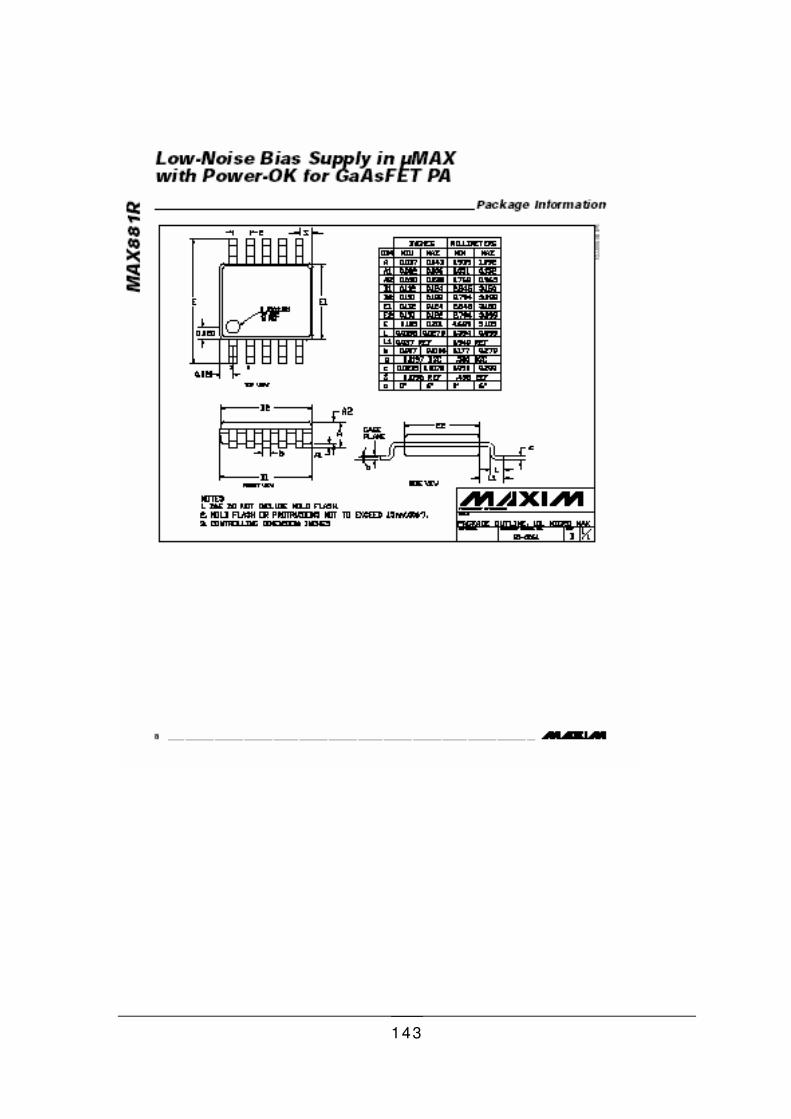
143

144
9 Appendix C
9.1 Support ive informat ion
Figure 44. Examples of matching foils for evaluation.
Chapter

145
Figure 45. Examples of device mounting inserts.