public finance: structural deficit, sensitivity and long ... finance: structural deficit,...

MINISTERO DELL’ECONOMIA E DELLE FINANZE

Study visit of the Delegation of the Government of Serbia

Rome, 23th January 2012

Public finance: structural deficit, sensitivity and long-term sustainability

Marco Cacciotti

MINISTERO DELL’ECONOMIA E DELLE FINANZE 2

Outline of the presentation The EU Stability and Growth pact

Theoretical underpinnings – fiscal rules

Legal requirements

Particular look at the Italian Stability and Convergence Programme:

Code of conduct

Structural deficits (derivation and results)

Sensitivity to growth (methodology and results)

Long-term sustainability of public finances (methodology and results)

Reform of the Stability and Growth Pact (ongoing) – some preliminary

elements.


Theoretical underpinnings EU – Stability and Growth Pact

Need for controlling

public finances.

High and persistent

government deficits may

lead to high and

unsustainable public

debt (increasing debt

before the Euro)

Other implicit liabilities

(such as ones due to

ageing) may lead to

increases in public

debts

As of 2007, effect of the

financial crisis on public

debts due to financial

support programmes.

0

20

40

60

80

100

120

140

160

180

19

91

19

92

19

93

19

94

19

95

19

96

19

97

19

98

19

99

20

00

20

01

20

02

20

03

20

04

20

05

20

06

20

07

20

08

20

09

20

10

20

11

20

12

Pu

bli

c D

eb

t (%

of

GD

P)

Debt/GDP in Europe

Euro area Germany Ireland Greece Spain France Italy

Source: European Commission, 2011 Spring Forecast



What are the costs of unsustainable public finances in the case of a single economy?

Piling up of public debt both in recession and in expansions

High interests rates to serve public debt

No fiscal space for automatic stabilisers to operate

High inflationary pressures and reduced macroeconomic stability

Crowding out of private investments.

Source: European Commission, 2011 Spring Forecast



What are the negative incentives for govermments to carry out deficit spending in the case of a

monetary union ?

Spillover effects on other members state of deficit spending carried out by single

countries

Increases of interest rates spread on the whole monetary union, given the inflation target.

Higher probability of an electoral cycle in budgetary spending

Risk of jeopardizing the activity and the credibility of the Central Bank

Need to foresee mechanisms that assure fiscal policy coordinations in the Monetary Union

Fiscal rules – Stability and Growth Pact (SGP)

Macro economic stability is a pre-requirement for accessing Euro Area.


Fiscal rules EU – Stability and Growth Pact

Fiscal rules are designed to impose quantitative constraints on public budgets (or part of them,

such as expenditures levels) aiming to:

permanently reduce the deficit bias and to impose a discipline on fiscal policy;

Minimize the probability of an electoral cycle of public spending

Increase the efficiency of public spending

Stabilise expectactions and the investment decisions of economic agents

Reduce the risk of pro-cyclical fiscal policies allowing the free operating of automatic

stabilisers.

Enhance the coordination of fiscal policies (weak institutional framework vis-à-vis fiscal

federalism).


Fiscal rules EU – Stability and Growth Pact

The provision of a fiscal rule does not always imply a better and more efficient fiscal

framework. The rule must be intertemporally credible and fully operative.

Ideally, a fiscal rule should be:

Well designed – clear juridical definition (Constitution or Law), clear specification of both ex ante and ex post

indicators, clear specification of the expenditures included (excluded) in (from) the fiscal aggregates;

Implementable: easy to apply, providing well designed procedures in cases of no compliance (either sanctions or

«escape clauses»);

Transparent: reduced possibility of «windows dressing» and reduced risk of creative accounting;

Simple: reference to numerical parameters easy to be controlloled by economic agents and financial markets;

Credible: targets should not be out of reach;

Consistent: fiscal rule should be in line with the objectives of monetary policy.


The European Framework – legislative references EU – Stability and Growth Pact

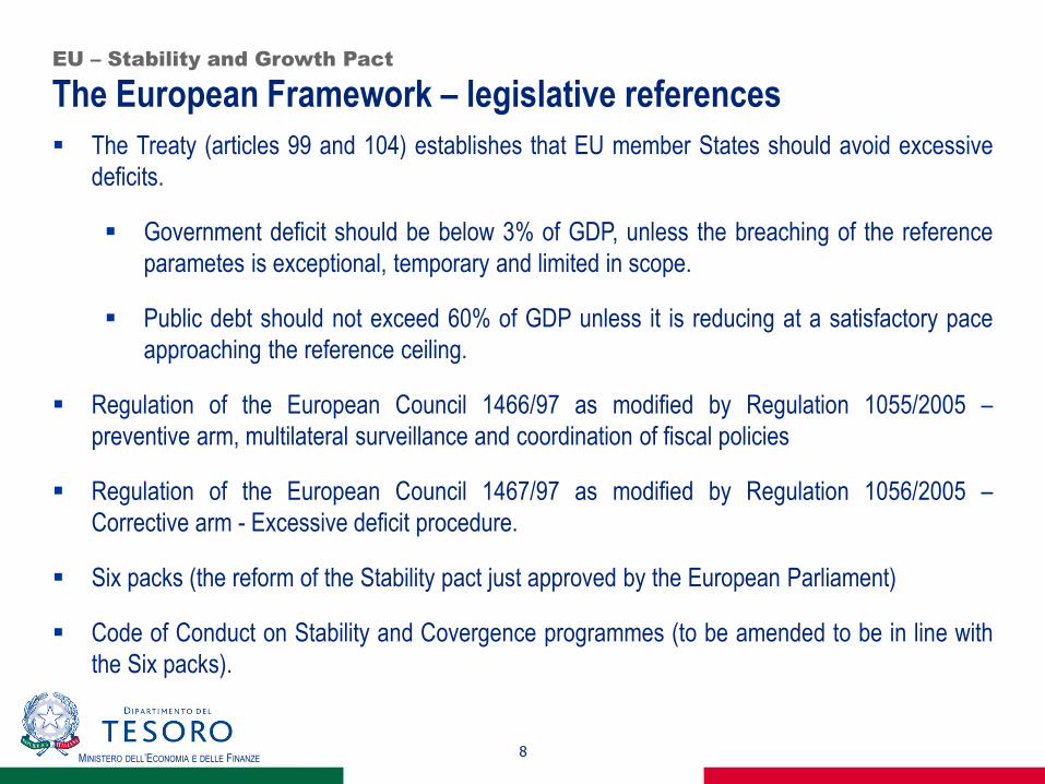
The Treaty (articles 99 and 104) establishes that EU member States should avoid excessive

deficits.

Government deficit should be below 3% of GDP, unless the breaching of the reference

parametes is exceptional, temporary and limited in scope.

Public debt should not exceed 60% of GDP unless it is reducing at a satisfactory pace

approaching the reference ceiling.

Regulation of the European Council 1466/97 as modified by Regulation 1055/2005 –

preventive arm, multilateral surveillance and coordination of fiscal policies

Regulation of the European Council 1467/97 as modified by Regulation 1056/2005 –

Corrective arm - Excessive deficit procedure.

Six packs (the reform of the Stability pact just approved by the European Parliament)

Code of Conduct on Stability and Covergence programmes (to be amended to be in line with

the Six packs).


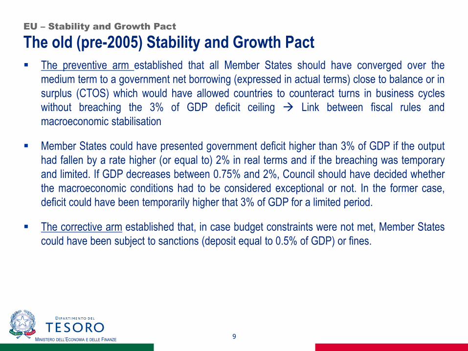
The old (pre-2005) Stability and Growth Pact EU – Stability and Growth Pact

The preventive arm established that all Member States should have converged over the

medium term to a government net borrowing (expressed in actual terms) close to balance or in

surplus (CTOS) which would have allowed countries to counteract turns in business cycles

without breaching the 3% of GDP deficit ceiling Link between fiscal rules and

macroeconomic stabilisation

Member States could have presented government deficit higher than 3% of GDP if the output

had fallen by a rate higher (or equal to) 2% in real terms and if the breaching was temporary

and limited. If GDP decreases between 0.75% and 2%, Council should have decided whether

the macroeconomic conditions had to be considered exceptional or not. In the former case,

deficit could have been temporarily higher that 3% of GDP for a limited period.

The corrective arm established that, in case budget constraints were not met, Member States

could have been subject to sanctions (deposit equal to 0.5% of GDP) or fines.


The 2005 version of the Stability and Growth Pact EU – Stability and Growth Pact

In 2002 Germany and France breached the deficit criterion. debate on more flexibility of SGP rules In march

2005 the European Council approved a reform of the SGP more rules and exemptions

Preventive arm

New parameters in the deficit criterion structural deficit (cyclically adjusted deficit net of one offs measures).

New rules country specific Medium term objectives (MTO), i.e. structural deficits linked to countries’ level of

initial debt and implicit liabilities (ageing expenditures). More flexibility for countries with low debt, reduced cost

of ageing and high potential

New rules member states far away from the MTOs should converge towards them by reducing the structural

deficit by at least 0.5 pp of GDP every years.

Assessement of one-off measures to counteract «windows dressing» and creative accounting.

Corrective arm

Less rigid definition of «severe economic crisis» based on potential output loss or reduced potential growth,

assessment of structural (pension reforms) and specific circumstances possibility to breach 3% of deficit/GDP

ratio.

Link to structural reforms and Lisbon Strategy.


The current version of the Stability and Growth Pact – the

European Semester.

EU – Stability and Growth Pact

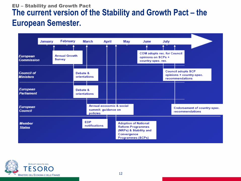
In 20010 introduction of the European Semester

The " European Semester " means the EU and the euro zone coordinate ex ante their budgetary

and economic policies, in line with both the Stability and Growth Pact and the Europe 2020

strategy.

The EU Semester starts with the Annual Growth Survey, in which the Commission provides a

solid analysis on the basis of the progress on Europe 2020 targets, and sets out an integrated

approach to recovery and growth, concentrating on key measures. This applies to the EU as a

whole and will then be translated into country-specific recommendations.

This procedure applies to the EU as a whole and is translated into country-specific

recommendations, thus allowing the ex ante economic coordination at EU level while national

budgets are still under preparation.


The current version of the Stability and Growth Pact – the

European Semester.

EU – Stability and Growth Pact


Requirements of the Code of Conduct Stability Programme

In the context of the European Semester, Member States every year submit to Commission

and Council the Stability and Convergence programmes.

Stability (Euro Area Countries) and Convergence programs (non Euro Area Countries) are

public documents submitted to Commission and Council, every year together with the National

Reform Programs, by mid-April. Commission and Council have to assess them and adopt

opinions and policy recommendations by end of July.

The Stability Program should follow the guidelines of the Annual Growth Survey and contain

the following info:

a) Actual and structural government balances and public debt planned for the medium

term (from t-1 to t+4);

b) Medium Term Objectives for budget (in structural terms);

c) the main underlying macroeconomic assumptions;

d) a description of the main budgetary measure to achieve the objectives and quality of

public finance.

e) sensitivity analysis on GDP growth assumptions and interest rates.

f) Long term sustainability of public finances.


Structural deficit

Why structural deficit?

General Government balance (in % of GDP) expressed in nominal terms is

subject to transitory (mainly cyclical) and permanent (istitutional) factors.

In order to use the fiscal levy in a counterciclycal fashion, policy-makers

should be able to disentagle business cycle influences on the budget.

Using goverment targets expressed in nominal terms may entail the risk that

that stabilization policies may turn out as being procyclical.


Estimation of the structural balance (SB) Structural deficit

The structural balance is defined as the general government balance, adjusted

for the cycle (CAB) and without one-off and other temporary measures.

[1]

The CAB (% GDP) is derived by subtracting from the headline general

government balance as a ratio to GDP(b) its cyclical component:

[2]

The budgetary sensitivity ε is the change in the general government balance

as a percent of GDP associated with an additional percentage point of output

gap. For Italy ε = 0.5.

The cyclical component is given by the product of ε and the Output Gap (OG).

Look at OG, ε and one-off measures.

ttt oneoffsCABSB

ttt OGbCAB


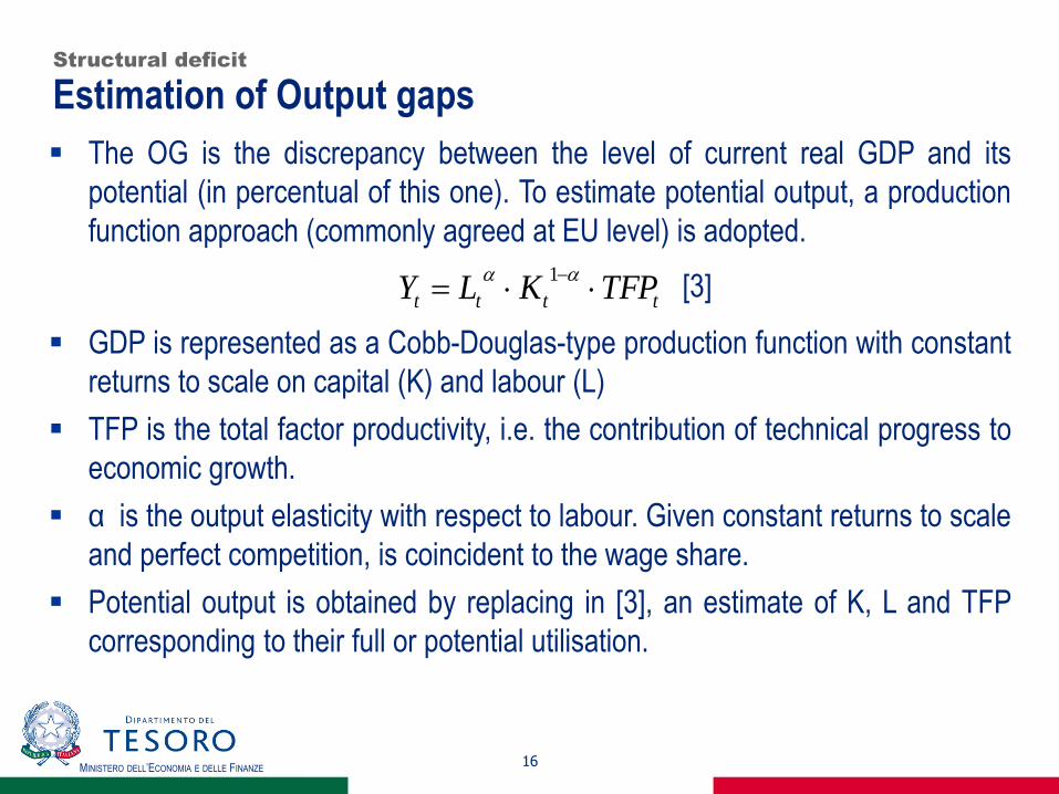
Estimation of Output gaps Structural deficit

The OG is the discrepancy between the level of current real GDP and its

potential (in percentual of this one). To estimate potential output, a production

function approach (commonly agreed at EU level) is adopted.

[3]

GDP is represented as a Cobb-Douglas-type production function with constant

returns to scale on capital (K) and labour (L)

TFP is the total factor productivity, i.e. the contribution of technical progress to

economic growth.

α is the output elasticity with respect to labour. Given constant returns to scale

and perfect competition, is coincident to the wage share.

Potential output is obtained by replacing in [3], an estimate of K, L and TFP

corresponding to their full or potential utilisation.

tttt TFPKLY

1


Estimation of Output gaps – Labour contribution to potential Structural deficit

The estimate of potential labour (LP) is achieved by smoothing a set of

exogenous variables over the historical sample and over a medium-term

extension period (usually 6y = a short-term forecast horizon + 3 year of

technical extrapolation so as to minimize the end-point-bias).

[4]

PARTS is the trend component of the unadjusted participation rate obtained by

Hodrick-Prescott (HP) filter.

POPW is the working-age population, extrapolated out of the sample period

using the Eurostat 2010 long range population projections.

HOURST is the trend of average hours worked per employee and it is

smoothed using an ARIMA process.

NAWRU is the non-accelerating wage rate of unemployment.

)1(*** ttttt NAWRUHOURSTPOPWPARTSLP


Estimation of Output gaps – NAWRU specification Structural deficit

NAWRU is derived by applying an unobserved component model estimated by

a Kalman filter.

The observed unemployment series is decomposed into a trend and a cyclical

component.

The trend component is modelled as a random walk with drift (the drift term

itself follows a random walk). The cyclical component is obtained via a Phillips

curve which regresses the change in wage inflation on cyclical unemployment

as well as on other exogenous variables (labour productivity, terms of trade

and wage share). In the out of sample extrapolation, the NAWRU is extended

over the forecast period by a mechanical rule which allows stabilising it after a

period of 3 years.


Estimation of Output gaps – Capital contribution to potential Structural deficit

Potential capital stock, measured by the perpetual inventory method,

corresponds to its actual value

The full utilisation of the existing stock is assumed.

The capital is extrapolated in the out-of-sample period according to a given

profile of productive investment (estimated through an AR(2) process) and

assuming a constant depreciation rate.


Estimation of Output gaps – TFP specification

Technical progress (TFP) is assumed to be propagated in a neutral way through qualitative

improvements both in labour and capital inputs.

TFP sums up both the level of efficiency of labour and capital inputs and their degree of

utilisation.

Structural deficit

))(( 11 KLKLt UUEETFP


Estimation of Output gaps – TFP contribution to potential Structural deficit

The long-run component of TFP is obtained through a a bivariate Kalman Filter (KF)

model which exploits the link between the TFP cycle and the degree of capacity

utilisation in the economy.

Its basic structure is similar to the Phillips-curve augmented unobserved component

model proposed by Kuttner (1994) for estimating potential output and output gaps in

the US.

Capacity utilization is measured using two indicators: the Capacity Utilization Indicator

(CUI), which is available for manufacturing only, and the Business Survey Capacity

Indicator (BS) collected for manufacturing, construction and services as part of the

European Commission's Business and Consumer Survey Programme.

TFP can be obtained by applying either a Maximum Likelihood or Bayesian (default

model) estimation techniques to the bivariate model in state-space specification given

by the Solow Residual (SR) (derived by replacing in equation [3] the observed value

of GDP, employment, hours worked and capital stock) and the series of Capacity

utilisation.


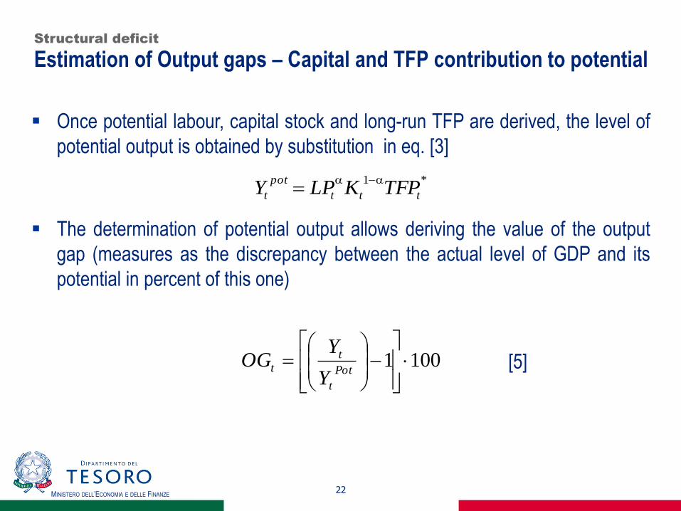
Estimation of Output gaps – Capital and TFP contribution to potential Structural deficit

Once potential labour, capital stock and long-run TFP are derived, the level of

potential output is obtained by substitution in eq. [3]

The determination of potential output allows deriving the value of the output

gap (measures as the discrepancy between the actual level of GDP and its

potential in percent of this one)

[5]

*1

ttt

pot

t TFPKLPY

1001

Pot

t

tt

Y

YOG


Estimation of the structural balance (SB) (II) – budget sensitivities Structural deficit

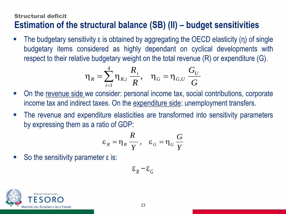
The budgetary sensitivity ε is obtained by aggregating the OECD elasticity (η) of single

budgetary items considered as highly dependant on cyclical developments with

respect to their relative budgetary weight on the total revenue (R) or expenditure (G).

On the revenue side we consider: personal income tax, social contributions, corporate

income tax and indirect taxes. On the expenditure side: unemployment transfers.

The revenue and expenditure elasticities are transformed into sensitivity parameters

by expressing them as a ratio of GDP:

So the sensitivity parameter ε is:

G

G

R

R U

UGG

i

i

iRR ,

4

1

, ,

Y

G

Y

RGGRR ,

GR


Estimation of the structural balance (SB) (III) – one-offs measures Structural deficit

One-offs are measures with a transitory budgetary effect that does not lead to a

sustained change in the intertemporal budgetary position

not exhaustive list: tax amnesties implying a one-off tax payment (to repatriate capital

from abroad); Sales of non-financial assets, typically real-estate, licences and

concessions; Legislative changes (permanent or temporary) with a temporary effect in

the timing of outlays or revenues; exceptional revenue linked to the transfer of pension

obligations; Exceptional revenue from state-owned companies; changes in revenue or

expenditure consecutive to Court or other authorities rulings; short-term emergency

costs associated with major natural catastrophes or other exceptional events;

Securitisation operations.


Estimation of the structural balance (SB) – Results for Italy – DEF – Stability

Programme (April 2011)

Structural deficit

In April 2011, structural deficit was expected to fall by 0,5 p.p. in the current year and by 0.8 p.p. the next,

getting to -2,2% of GDP at the end of 2012, in line with the commitments agreed at a European level .

In 2013 and 2014, as a result of additional fiscal measures announced by the government (amounting,

cumulatively to 2.3 percentage points of GDP) cyclically adjusted budget balance, net of one-off measures,

should have continued to fall by 0.8 p.p. per year.

Italy was expected to reach the Medium Term Objective (MTO) by 2014.

2009 2010 2011 2012 2013 2014

GDP growth rate at constant prices -5,2 1,3 1,1 1,3 1,5 1,6

Net borrowing -5,4 -4,6 -3,9 -2,7 -1,5 -0,2

Interest payments 4,6 4,5 4,8 5,1 5,4 5,5

Potential GDP growth rate -0,1 0,1 0,3 0,4 0,6 0,8

Contribution of productive factors to potential growth

Labour 0,0 0,1 0,1 0,1 0,2 0,2

Capital 0,2 0,2 0,3 0,3 0,3 0,4

Total factor productivity -0,4 -0,2 -0,1 0,0 0,1 0,2

Output gap -3,9 -2,7 -1,9 -1,1 -0,3 0,5

Cyclical budgetary component -1,9 -1,3 -1,0 -0,6 -0,1 0,3

Cyclically-adjusted budget balance -3,5 -3,3 -2,9 -2,2 -1,3 -0,5

Cyclically-adjusted primary surplus 1,2 1,3 1,9 2,9 4,0 5,0

One-off measures 0,7 0,2 0,1 0,1 0,0 0,0

Budget balance, net of one-off measures -6,0 -4,8 -4,0 -2,8 -1,5 -0,3

Cyclically-adjusted budget balance, net of one-off measures -4,1 -3,5 -3,0 -2,2 -1,4 -0,5

Cyclically-adjusted primary surplus, net of one-off measures 0,5 1,1 1,8 2,9 4,0 4,9

Change in budget balance, net of one-off measures 3,1 -1,2 -0,8 -1,2 -1,3 -1,2

Change in cyclically-adjusted budget balance, net of one-off measures 0,5 -0,6 -0,5 -0,8 -0,8 -0,8


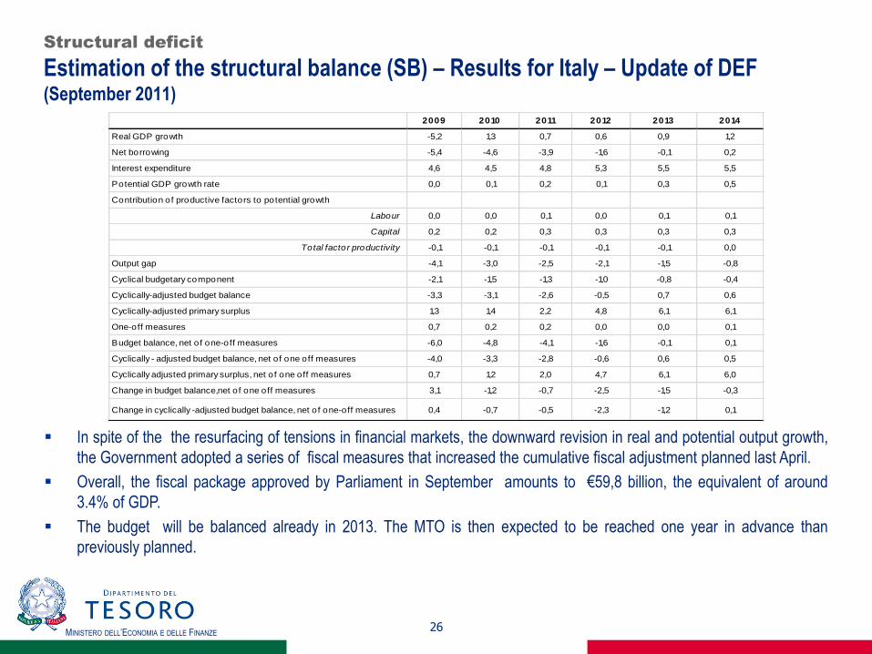
In spite of the the resurfacing of tensions in financial markets, the downward revision in real and potential output growth,

the Government adopted a series of fiscal measures that increased the cumulative fiscal adjustment planned last April.

Overall, the fiscal package approved by Parliament in September amounts to €59,8 billion, the equivalent of around

3.4% of GDP.

The budget will be balanced already in 2013. The MTO is then expected to be reached one year in advance than

previously planned.

26

2009 2010 2011 2012 2013 2014

Real GDP growth -5,2 1,3 0,7 0,6 0,9 1,2

Net borrowing -5,4 -4,6 -3,9 -1,6 -0,1 0,2

Interest expenditure 4,6 4,5 4,8 5,3 5,5 5,5

Potential GDP growth rate 0,0 0,1 0,2 0,1 0,3 0,5

Contribution of productive factors to potential growth

Labour 0,0 0,0 0,1 0,0 0,1 0,1

Capital 0,2 0,2 0,3 0,3 0,3 0,3

Total factor productivity -0,1 -0,1 -0,1 -0,1 -0,1 0,0

Output gap -4,1 -3,0 -2,5 -2,1 -1,5 -0,8

Cyclical budgetary component -2,1 -1,5 -1,3 -1,0 -0,8 -0,4

Cyclically-adjusted budget balance -3,3 -3,1 -2,6 -0,5 0,7 0,6

Cyclically-adjusted primary surplus 1,3 1,4 2,2 4,8 6,1 6,1

One-off measures 0,7 0,2 0,2 0,0 0,0 0,1

Budget balance, net of one-off measures -6,0 -4,8 -4,1 -1,6 -0,1 0,1

Cyclically - adjusted budget balance, net of one off measures -4,0 -3,3 -2,8 -0,6 0,6 0,5

Cyclically adjusted primary surplus, net of one off measures 0,7 1,2 2,0 4,7 6,1 6,0

Change in budget balance,net of one off measures 3,1 -1,2 -0,7 -2,5 -1,5 -0,3

Change in cyclically -adjusted budget balance, net of one-off measures 0,4 -0,7 -0,5 -2,3 -1,2 0,1

Structural deficit

Estimation of the structural balance (SB) – Results for Italy – Update of DEF (September 2011)


Sensitivity analysis – net borrowing and debt in alternative scenarios

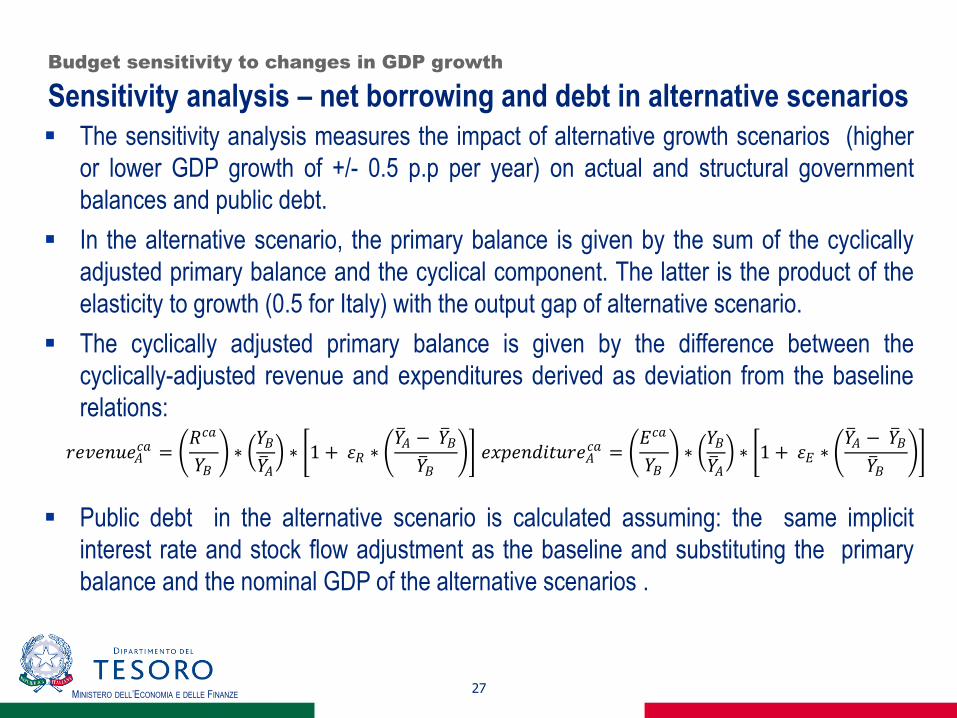
The sensitivity analysis measures the impact of alternative growth scenarios (higher

or lower GDP growth of +/- 0.5 p.p per year) on actual and structural government

balances and public debt.

In the alternative scenario, the primary balance is given by the sum of the cyclically

adjusted primary balance and the cyclical component. The latter is the product of the

elasticity to growth (0.5 for Italy) with the output gap of alternative scenario.

The cyclically adjusted primary balance is given by the difference between the

cyclically-adjusted revenue and expenditures derived as deviation from the baseline

relations:

Public debt in the alternative scenario is calculated assuming: the same implicit

interest rate and stock flow adjustment as the baseline and substituting the primary

balance and the nominal GDP of the alternative scenarios .

Budget sensitivity to changes in GDP growth

𝑟𝑒𝑣𝑒𝑛𝑢𝑒𝐴𝑐𝑎 =

𝑅𝑐𝑎

𝑌𝐵 ∗

𝑌𝐵

𝑌 𝐴 ∗ 1 + 𝜀𝑅 ∗

𝑌 𝐴 − 𝑌 𝐵

𝑌 𝐵 𝑒𝑥𝑝𝑒𝑛𝑑𝑖𝑡𝑢𝑟𝑒𝐴

𝑐𝑎 = 𝐸𝑐𝑎

𝑌𝐵 ∗

𝑌𝐵

𝑌 𝐴 ∗ 1 + 𝜀𝐸 ∗

𝑌 𝐴 − 𝑌 𝐵

𝑌 𝐵


Sensitivity analysis – net borrowing/GDP in alternative scenarios –

DEF – Stability Programme (May 2011)


-6,0

-5,0

-4,0

-3,0

-2,0

-1,0

0,0

1,0

2011 2012 2013 2014

High-growth scenario Baseline scenario Low-growth scenario


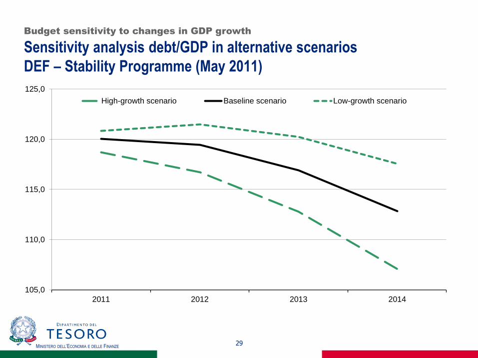
Sensitivity analysis debt/GDP in alternative scenarios



105,0

110,0

115,0

120,0

125,0

2011 2012 2013 2014

High-growth scenario Baseline scenario Low-growth scenario


Sustainability of Public finances- Public debt projections

Long term sustainability of public finances presents both the evolution of the

debt/GDP ratio up till 2060 as a function of age-related expenditure projections and

sustainability indicators (S1 and S2).

Age-related expenditures are: pensions (projected through national models), healt-

care and long term care outlays, education expenditures and unemployment benefits

(projected by the European Commission on the basis of commonly agreed models

and assumptions).

The underlying macroeconomic and demographic assumptions and age-related

expenditures are agreed at EU level (Ageing Working Group – 2009 Ageing Report).

Tax revenue are kept constant at the level (in term of GDP) resulting from the last year

of the Stability Programme (2014). Structural primary balance and debt change

according to the evolution of age related expenditures.

[6]

Long term debt dynamics

01 1 t t t t t t td d r d pb pi are


Long-term projections of revenues and expenditure (may 2010)

LONG-TERM SUSTAINABILITY OF PUBLIC FINANCES

In order to take the effects of the crisis into account, the underlying macroeconomic outlook assumes the “lost decade

scenario” in which labour productivity converges to the AWG baseline scenario by 2020.

Total expenditures are projected to increase in 2010 as an effect of the crisis and then decrease up till the level of

45.0% of GDP in 2060. Pension expenditure are expected to increase in the medium term and then decrease. As a

result of the crisis, healthcare expenditure will be on a higher level than compared to last year projections but its

dynamic would not change.

2005 2010 2015 2020 2025 2030 2035 2040 2045 2050 2055 2060

Total expenditure 48,2 50,6 48,1 47,0 46,2 46,1 46,2 46,7 47,0 46,4 45,8 45,0

of which: age-related expenditure 26,1 28,6 27,9 27,5 27,4 27,9 28,3 29,0 29,3 28,9 28,6 28,2

Pension expenditure 14,0 15,3 15,4 15,1 14,9 15,2 15,4 15,7 15,6 14,9 14,3 13,9

of which: seniority and old-age pensions 13,4 14,8 14,9 14,6 14,5 14,8 15,0 15,4 15,3 14,6 14,0 13,6

of which: other pensions (disability and survivors) 0,6 0,5 0,5 0,5 0,5 0,4 0,4 0,3 0,3 0,3 0,3 0,3

Healthcare expenditure 6,7 7,3 7,3 7,4 7,6 7,9 8,1 8,4 8,6 8,7 8,8 8,8

Long-term care expenditure 0,8 1,0 1,0 1,0 1,1 1,1 1,2 1,3 1,4 1,5 1,6 1,7

Education expenditure 4,2 4,2 3,7 3,5 3,4 3,2 3,2 3,2 3,3 3,3 3,4 3,4

Unemployment benefits 0,4 0,7 0,5 0,4 0,4 0,4 0,4 0,4 0,4 0,4 0,4 0,4

Interest expenditure 4,5 4,9 5,2 4,5 3,8 3,3 2,9 2,7 2,6 2,5 2,2 1,8

Total revenues 43,8 46,0 45,9 45,8 45,8 45,8 45,8 45,8 45,8 45,7 45,7 45,7

of which: property income 0,6 0,6 0,6 0,6 0,6 0,5 0,5 0,5 0,5 0,5 0,5 0,5

% GDP


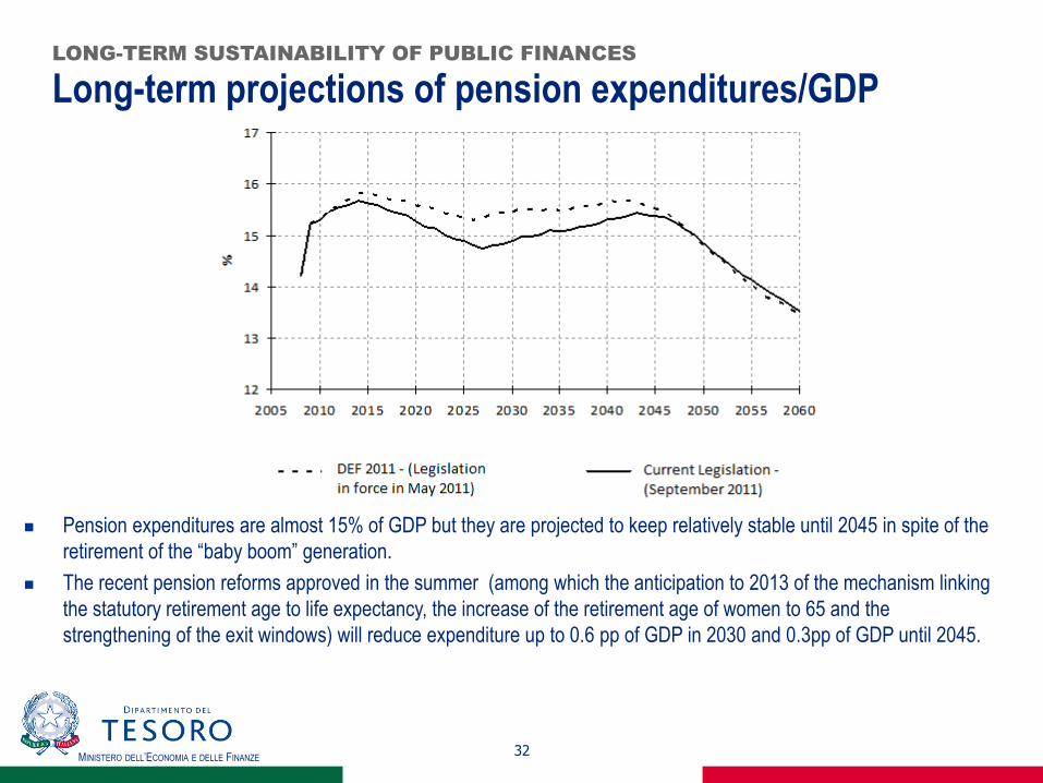
Long-term projections of pension expenditures/GDP LONG-TERM SUSTAINABILITY OF PUBLIC FINANCES

Pension expenditures are almost 15% of GDP but they are projected to keep relatively stable until 2045 in spite of the

retirement of the “baby boom” generation.

The recent pension reforms approved in the summer (among which the anticipation to 2013 of the mechanism linking

the statutory retirement age to life expectancy, the increase of the retirement age of women to 65 and the

strengthening of the exit windows) will reduce expenditure up to 0.6 pp of GDP in 2030 and 0.3pp of GDP until 2045.


Debt to GDP projections under alternative assumptions



The fiscal targets planned by the government in May will bring the debt/GDP ratio over a descending path over

the long term.

The adoption of labour market reforms spurring productivity will automatically improve the sustainability of public

finances over the long term. In case of negative shocks in labour productivity, the sustainability is not at risk.

-60

-30

0

30

60

90

120

201

4

201

6

201

8

202

0

202

2

202

4

202

6

202

8

203

0

203

2

203

4

203

6

203

8

204

0

204

2

204

4

204

6

204

8

205

0

205

2

205

4

205

6

205

8

206

0

baseline

productivity +0.2 p.p. from 2015

productivity -0.2 p.p. from 2015

female activity rate +5% in 2060


Sustainability indicators: S1 and S2 LONG-TERM SUSTAINABILITY OF PUBLIC FINANCES

S2 measures the structural primary balance permanent adjustment that would allow to

fullfil the intertemporal budget constraint over an infinite horizon.

[7]

S2 can be decomposed in two sub-indicators:

D (initial budgetary position) it quantifies the permanent adjustment in the structural

primary balance which is needed to keep the debt/GDP ratio constant at its initial

value (dt0) by offsetting the snowball effect (the built up of interest expenditures). The

technical assumption is that there are no age-related changes in the primary balance

(Δpbs=0).

E (long-term changes in the primary balance) measures the permanent adjustment in

the structural primary balance that it is needed to offset the cost of ageing (implicit

liabilities).

0 0

0 1--------------------- ------------------------------------

2 1t t s s

s t

D E

S rd pb w pb

0

0

0 1

1

1

s t

ss t

s t

rw

r


35

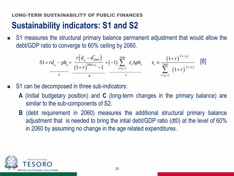
Sustainability indicators: S1 and S2


S1 measures the structural primary balance permanent adjustment that would allow the

debt/GDP ratio to converge to 60% ceiling by 2060.

[8]

S1 can be decomposed in three sub-indicators:

A (initial budgetary position) and C (long-term changes in the primary balance) are

similar to the sub-components of S2.

B (debt requirement in 2060) measures the additional structural primary balance

adjustment that is needed to bring the intial debt/GDP ratio (dt0) at the level of 60%

in 2060 by assuming no change in the age related expenditures.

0

0 0 0

0

*2060

2060

20601

--------------------- ------------------------------------------------------------------------

1 11 1

t

t t s sts t

A B

r d dS rd pb z pb

r

C

0

0

0

2060

1

1

1

s t

ss t

s t

rz

r


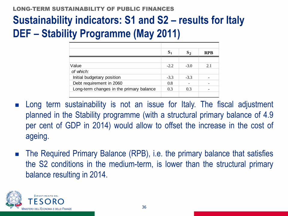
Sustainability indicators: S1 and S2 – results for Italy



Long term sustainability is not an issue for Italy. The fiscal adjustment

planned in the Stability programme (with a structural primary balance of 4.9

per cent of GDP in 2014) would allow to offset the increase in the cost of

ageing.

The Required Primary Balance (RPB), i.e. the primary balance that satisfies

the S2 conditions in the medium-term, is lower than the structural primary

balance resulting in 2014.

S1 S2 RPB

Value -2.2 -3.0 2.1

of which:

Initial budgetary position -3.3 -3.3 -

Debt requirement in 2060 0.8 - -

Long-term changes in the primary balance 0.3 0.3 -


The Medium term budgetary objective (MTO)

MTO is a country-specific indicator defined in cyclically adjusted terms, net of one-off and

other temporary measures.

MTOs derivation must take into account of three components:

The debt-stabilising balance for a debt ratio equal to the (60% of GDP) reference value

(dependent on long-term potential growth), implying room for budgetary manoeuvre for

member States with relatively low debt;

A supplementary debt reduction for Member State with a debt ratio (60% of GDP) in

excess of the reference value, implying rapid progress towards it;

A fraction of the adjustment needed to cover the present value of the future increase in

age-related government expenditure.

37

THE IMPLEMENTATION OF THE STABILITY AND GROWTH PACT


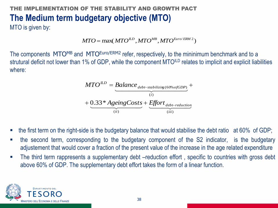
The Medium term budgetary objective (MTO) MTO is given by:

The components MTOMB and MTOEuro/ERM2 refer, respectively, to the mininimum benchmark and to a

strutural deficit not lower than 1% of GDP, while the component MTOILD relates to implicit and explicit liabilities

where:

the first term on the right-side is the budgetary balance that would stabilise the debt ratio at 60% of GDP;

the second term, corresponding to the budgetary component of the S2 indicator, is the budgetary

adjustement that would cover a fraction of the present value of the increase in the age related expenditure

The third term rappresents a supplementary debt –reduction effort , specific to countries with gross debt

above 60% of GDP. The supplementary debt effort takes the form of a linear function.

38

)()(

)(

)%60(

*33.0

iii

reductiondebt

ii

i

ofGDPgstabilizindebt

ILD

EffortsAgeingCost

BalanceMTO

THE IMPLEMENTATION OF THE STABILITY AND GROWTH PACT

),,max( 2/ ERMEuroMBILD MTOMTOMTOMTO


Adjustment path toward the Medium-term budgetary objective (MTO)

Member States far away from the MTO should converge towards it by reducing the

structural deficit by 0.5 pp per year. After the crisis, this mechanism has been reinforced.

The presumption is to use the unexpected extra revenues windfalls for deficit and debt

reduction while keeping expenditure on a stable sustainable path over the cycle.

The Commission and the Council will assess the growth path of government expenditure

against a reference medium term rate of potential GDP growth.

For countries far away from the their MTO, public expenditures can grow at a rate well

below the reference medium-term rate of potential GDP (unless covered by increases in

discretionary revenues) so that the structural deficit falls by at least 0.5pp every years.

Member States at the MTO can leave expenditure grow at the same rate of the reference

potential GDP.

The reference medium-term rate of potential GDP growth is based on both forward-

looking and backward-looking estimates (t-5, t+5).

39

THE REFORM OF THE STABILITY AND GROWTH PACT


The Excessive deficit procedure – The debt rule

In addition to deficit, the Commission has to examine compliance with budgetary discipline on the

basis of debt criteria (reference to 60% of Debt/GDP).

Accordingly, the Commission will always prepare a report for Excessive Deficit Procedure a report

when at least one of the conditions (1) or (2) holds:

A planned government deficit exceeds the reference value of 3% of GDP

A reported government debt ratio is above the reference value of 60% of GDP and its differential w.r.t. the

reference value has not decreased over the past three years at a rate of one-twentieth as a benchmark, which is

measured by an excess of the debt ratio reported for the year t over a backward looking element of a benchmark

(but also some forward-looking elements will be taken into account).

40

THE REFORM OF THE STABILITY AND GROWTH PACT

public finance: structural deficit, sensitivity and long ... finance: structural deficit,...

Documents