public disclosure authorized wps3682 - world...

The Poverty and Distributional Impact of Macroeconomic Shocks and Policies:

A Review of Modeling Approaches

B. Essama-Nssah

Poverty Reduction Group The World Bank Washington, DC

Abstract The importance of distributional issues in policy making creates a need for empirical tools to assess the social impact of economic shocks and policies. This paper reviews some of the modeling approaches that are currently in use at the World Bank and other international financial institutions. The specification of these models is dictated by the issues at stake, the knowledge about the nature of the process involved, and the availability and reliability of relevant data. Furthermore, shocks and policies have macroeconomic, structural, and distributional implications. This creates interdependence between such policy issues. Finally, the distributional impact of shocks and policies hinges on the heterogeneity of socioeconomic agents with respect to endowments and behavior. In the end, each modeling approach should be judged on how well it handles the interdependence between policy issues and the heterogeneity of the stakeholders, given other constraints.

World Bank Policy Research Working Paper 3682, August 2005 The Policy Research Working Paper Series disseminates the findings of work in progress to encourage the exchange of ideas about development issues. An objective of the series is to get the findings out quickly, even if the presentations are less than fully polished. The papers carry the names of the authors and should be cited accordingly. The findings, interpretations, and conclusions expressed in this paper are entirely those of the authors. They do not necessarily represent the view of the World Bank, its Executive Directors, or the countries they represent. Policy Research Working Papers are available online at http://econ.worldbank.org.

This paper is part of a larger effort to provide operational guidance on the analysis of the distributional implications of policy reforms. For further details, please visit www.worldbank.org/psia. The author is grateful to Stefano Paternostro, Aline Coudouel, Vijdan Korman, Moataz Mostafa Kamel El Said, Hans Löfgren, Delfin S. Go, Oleksiy Ivaschenko, David P. Coady, Limin Wang, and Philippe H. Le Houerou for useful suggestions and insightful comments on an earlier draft of this paper. Vijdan also provided excellent support for the preparation of this version of the paper.

WPS3682

Pub

lic D

iscl

osur

e A

utho

rized

Pub

lic D

iscl

osur

e A

utho

rized

Pub

lic D

iscl

osur

e A

utho

rized

Pub

lic D

iscl

osur

e A

utho

rized

Pub

lic D

iscl

osur

e A

utho

rized

Pub

lic D

iscl

osur

e A

utho

rized

Pub

lic D

iscl

osur

e A

utho

rized

Pub

lic D

iscl

osur

e A

utho

rized

1

Table of Contents 1. Introduction..................................................................................................................... 2 2. Simulation Models of the Size Distribution of Income .................................................. 7

2.1. The Lorenz Curve Approach ................................................................................... 8 POVCAL..................................................................................................................... 8 SimSIP Poverty......................................................................................................... 11

2.2. Unit-Record-Based Approaches ............................................................................ 13 PovStat ...................................................................................................................... 13 The Envelope Model................................................................................................. 16 The Household Income and Occupational Choice Model ........................................ 19

3. Embedding Distributional Mechanisms within a General Equilibrium Model ............ 23 3.1. The Logic of General Equilibrium Modeling ........................................................ 23

What is a General Equilibrium Model? .................................................................... 23 Empirical Implementation ........................................................................................ 24

3.2. Modeling Distributional Mechanisms.................................................................... 28 4. Linking a Macroeconomic Framework to a Model of Income Distribution................. 31

4.1. The 123PRSP Model ............................................................................................. 32 The Financial Programming Module ........................................................................ 33 The Growth Module.................................................................................................. 35 The Two-Sector General Equilibrium Model ........................................................... 36 The Micro-Layer....................................................................................................... 39

4.2. The PAMS Framework .......................................................................................... 42 The RMSM-X Module.............................................................................................. 42 The Meso-Module..................................................................................................... 44 The Poverty Simulator .............................................................................................. 46 Operational Support .................................................................................................. 47 Reduced-Form Implementation ................................................................................ 47

4.3. A Macro-Micro Simulation Model for Brazil........................................................ 49 The IS-LM Model ..................................................................................................... 49 Linkage Variables ..................................................................................................... 50

4.4. The IMMPA Framework ....................................................................................... 50 The Labor Market ..................................................................................................... 51 The Financial Sector ................................................................................................. 52 Public Expenditure.................................................................................................... 52 Distributional Analysis ............................................................................................. 52

5. Concluding Remarks..................................................................................................... 54 Annex................................................................................................................................ 56 Notes ................................................................................................................................. 65 References......................................................................................................................... 67

2

1. Introduction The importance of distributional issues in policy making creates a need for

empirical tools to assess the impact of economic shocks and policies on the living

standards of relevant individuals. The purpose of this paper is therefore to review some of

the modeling approaches that are currently in use at the World Bank and other

international financial institutions in the evaluation of the impact of macroeconomic

shocks and policies on poverty and income distribution. The hope is that the interested

reader might then be able to make an informed choice from among the alternative

approaches.1

Developing countries face a host of macroeconomic challenges in the design and

implementation of development strategies and policies. Some of the recurrent issues

include (1) fiscal adjustment, (2) monetary policy reforms, (3) trade liberalization, and

(4) the impact of terms-of-trade shocks. Fiscal adjustment involves a modification of

government tax, spending, and borrowing policies to achieve a sustainable

macroeconomic framework consistent with the objectives of economic growth and

poverty reduction. Monetary policy reforms entail control of foreign capital flows and

adjustments in the money supply and in the exchange rate. Trade liberalization implies a

reduction or removal of trade barriers such as quantitative restrictions and tariffs. In fact,

trade liberalization has become a prerequisite for participation in the World Trade

Organization. Finally, terms-of-trade shocks are important determinants of the

performance of open economies. Many developing countries are indeed primary

commodity exporters or net oil importers and hence vulnerable to volatility in the world

prices of these commodities.

The need to consider the distributional implications of such macroeconomic

events stems from at least two basic considerations related to the goal of development and

the heterogeneity of the stakeholders. In the context of the Millennium Declaration

(United Nations 2000), the international community has included poverty and hunger

eradication among the basic objectives of development and has thus made poverty

reduction a benchmark measure of the performance of socioeconomic systems. This

vision is consistent with the notion of development as empowerment, meaning a process

that entails the expansion of the ability of the participants to achieve their freely chosen

3

life plans. In this perspective, poverty is seen as the deprivation of basic capabilities to

live the kind of life that one has reason to value (Sen 1999).

Furthermore, political factors are essential determinants of economic outcomes,

and distributional issues underpin the political dimension of policy making (understood

to include implementation) because of the heterogeneity of interests. Heterogeneity may

stem from differences in tastes, in resource endowments, or in the view of the world.

There could be conflicts of interests even in situations where the socioeconomic agents

are identical ex ante. They may value a good equally, yet be in conflict over the

distribution of the good (Drazen 2000). Approaches to policy making may be

characterized according to whether they account for political constraints arising from a

heterogeneity of interests. With no conflict of interests, optimal policies could be found

by maximizing the utility of a representative agent. This is essentially the normative

approach to policy making (Dixit 1996). In the positive approach, policy making is

viewed as a political process involving strategic interactions among various

socioeconomic agents subject to potential conflict over distribution.

Two basic dimensions define the desirable properties of a policy model: relevance

and reliability (Quade 1982). A relevant model focuses on issues of concern and on

politically significant socioeconomic groups and the interactions among them. A reliable

model is based on sound analytical linkages between available policy instruments (part of

the exogenous variables) and relevant outcomes, for example, poverty or inequality (part

of the endogenous variables), so as to ensure a high degree of confidence in the model’s

predictions. Modeling the poverty and distributional impacts of macroeconomic shocks

and policies therefore requires a clear understanding of the transmission channels. This

relates to the specification of the linkages between macroeconomic shocks and policies,

as well as the fundamental determinants of the distribution of economic welfare. In the

terminology of Bourguignon, Ferreira, and Lustig (2005), macroeconomic events may

have three types of effects on income distribution: (1) endowment effects represent

changes in the amounts of the resources available to individuals or households; (2) price

effects translate changes in the remuneration of these resources; (3) finally, occupational

effects represent changes in resource allocation.

The outline of the paper is as follows. Section 2 focuses on simulation models of

4

the size distribution of an indicator of economic welfare. In the section, we review two

types of approaches to modeling the size distribution of economic welfare across a

population. The first includes purely statistical models such as POVCAL (Chen, Datt, and

Ravallion 1991) and SimSIP Poverty (Wodon, Ramadas, and van der Mensbrugghe

2003). These two tools rely on a parameterization of the Lorenz curve and, arguably,

offer the simplest way of simulating the poverty effect of macroeconomic shocks and

policies. The second approach relies on unit record data and includes (1) PovStat (Datt

and Walker 2002), (2) the maximum value or envelope model2 (Chen and Ravallion 2004;

Ravallion and Lokshin 2004), and (3) the household income and occupational choice

model (Bourguignon and Ferreira 2005).

Section 3 discusses poverty and distributional analysis within a general

equilibrium framework (Dervis, de Melo, and Robinson 1982; Decaluwé and others

1999).

Section 4 reviews modular approaches to linking macroeconomic models to

models of income distribution. The section focuses on the 123PRSP model – the name

stands for one country, two sectors, and three commodities, and the model is built to feed

into the macroeconomic framework for Poverty Reduction Strategy Papers – (Devarajan

and Go 2003); the Poverty Analysis Macroeconomic Simulator I (PAMS I) (Pereira da

Silva, Essama-Nssah, and Samaké 2003); PAMS II (Essama-Nssah 2004); a macro-micro

simulation model for Brazil that uses the investment savings–liquidity money (IS-LM)

framework for macroeconomic analysis (Ferreira and others 2004); and the integrated

macroeconomic model for poverty analysis (IMMPA) framework, which links a dynamic

computable general equilibrium (CGE) model to unit record data (Agénor, Izquierdo, and

Jensen, forthcoming).

Concluding remarks are presented in Section 5. An annex provides a summary

description of the tools reviewed in this paper.

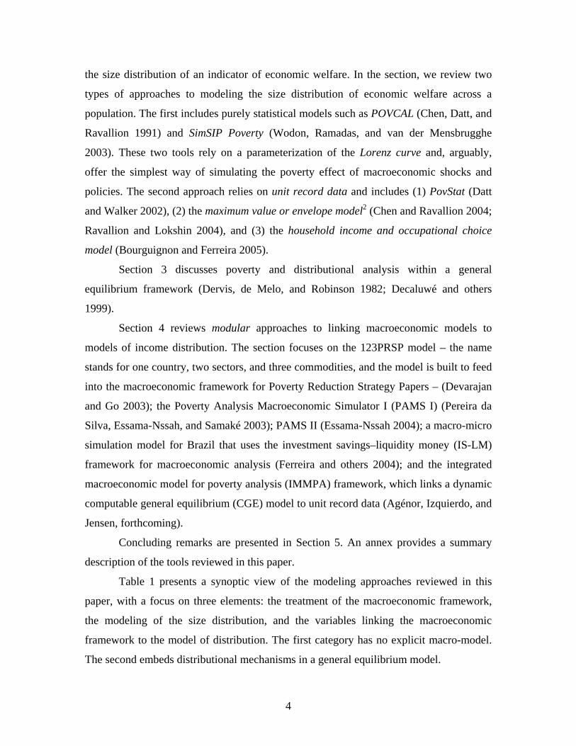
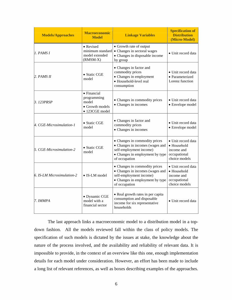
Table 1 presents a synoptic view of the modeling approaches reviewed in this

paper, with a focus on three elements: the treatment of the macroeconomic framework,

the modeling of the size distribution, and the variables linking the macroeconomic

framework to the model of distribution. The first category has no explicit macro-model.

The second embeds distributional mechanisms in a general equilibrium model.

5

Table 1. Modeling the Poverty and Distributional Impacts of Macroeconomic

Shocks and Policies

Models/Approaches Macroeconomic Model Linkage Variables

Specification of Distribution

(Micro-Model)

A. Distributional Focus (No Explicit Macro-Model)

Lorenz Curve Approach

1. POVCAL • Implicit • Mean consumption/income of the distribution

• Parameterized Lorenz function

2. SimSIP Poverty • Implicit • Mean consumption/income of the distribution

• Parameterized Lorenz function

Unit Record Approach

1. PovStat • Implicit

• Per capita household consumption • Sector of employment of the household head • Growth rate of per capita output in the sector of employment

• Unit record data

2. The Envelope Model (Microsimulation-1) • Implicit

• Changes in supply prices for household production activities • Changes in demand prices • Changes in incomes


3. Household Income and Occupational Choice Models (Microsimulation-2)

• Implicit

• Changes in commodity prices • Changes in incomes (wages and self-employment income) • Changes in employment by type of occupation


B. Standard General Equilibrium Analysis

1. CGE–Representative Household • Static CGE

• Changes in factor and commodity prices • Changes in employment

• A few representative households

2. CGE–Extended Representative Household • Static CGE

• Changes in factor and commodity prices • Changes in employment

• A few representative households • A model of size distribution

C. Sequential Macro-Micro Linkages

6

Models/Approaches Macroeconomic Model Linkage Variables

Specification of Distribution

(Micro-Model)

1. PAMS I

• Revised minimum standard model extended

(RMSM-X)

• Growth rate of output • Changes in sectoral wages • Changes in disposable income by group


2. PAMS II • Static CGE model

• Changes in factor and commodity prices • Changes in employment • Household-level real consumption

• Unit record data • Parameterized Lorenz function

3. 123PRSP

• Financial programming model • Growth models • 123CGE model

• Changes in commodity prices • Changes in incomes

• Unit record data • Envelope model

4. CGE-Microsimulation-1 • Static CGE model

• Changes in factor and commodity prices • Changes in incomes

• Unit record data • Envelope model

5. CGE-Microsimulation-2 • Static CGE model


• Unit record data • Household income and occupational choice models

6. IS-LM Microsimulation-2 • IS-LM model


• Unit record data • Household income and occupational choice models

7. IMMPA • Dynamic CGE model with a financial sector

• Real growth rates in per capita consumption and disposable income for six representative households


The last approach links a macroeconomic model to a distribution model in a top-

down fashion. All the models reviewed fall within the class of policy models. The

specification of such models is dictated by the issues at stake, the knowledge about the

nature of the process involved, and the availability and reliability of relevant data. It is

impossible to provide, in the context of an overview like this one, enough implementation

details for each model under consideration. However, an effort has been made to include

a long list of relevant references, as well as boxes describing examples of the approaches.

7

In addition, the annex supplies a description of many of the tools considered. It also

includes information on the cost of implementation and appropriate software for some of

the tools.

2. Simulation Models of the Size Distribution of Income The idea of simulating the distribution of income among individuals or

households originated in the field of public finance because of the need to have reliable

models for the detailed analysis of the incidence of a tax-benefit system. The basic idea is

to model the distribution of household income and consumption taking household

behavior as exogenous, but fully accounting for applicable taxes and transfers (Davies

2004). To take full account of the diversity of the characteristics in a population, these

simulation models require a nationally representative micro-data set. The fact that

household behavior is exogenous means that these accounting models can predict only

the first-round effects of a tax-benefit policy on inequality and poverty.

All the approaches reviewed in this section are various interpretations of the basic

idea underlying tax-benefit simulation models. POVCAL and SimSIP Poverty illustrate

the use of the Lorenz curve for poverty and distributional impact analysis. These two

tools are particularly useful when only aggregate or grouped data are available. The

second class of simulation tools considered under this heading relies on unit record data

on the distribution of some money-metric measure of economic welfare at the individual

or household level. Three approaches are examined. PovStat uses per capita consumption

as a measure of welfare. The second approach relies on the envelope theorem and

employs the maximum value function to model the determinants of individual welfare

(Chen and Ravallion 2004; Ravallion and Lokshin 2004). The last approach is based on a

reduced-form model of household income generation (Bourguignon and Ferreira 2005).

Even though the envelope model and the income-generation models include some aspects

of household behavior, these microsimulation models must be viewed as statistical

devices to the extent that they fail to fully account for market adjustment through

endogenous prices or the adjustment of the behavior of agents from one equilibrium state

to another (Ferreira and Leite 2003).

8

2.1. The Lorenz Curve Approach Given that poverty indexes are computed on the basis of a distribution of living

standards that is fully characterized by the mean and by the degree of inequality, it is

reasonable to think of a poverty indicator as a function of these two factors. In fact,

procedures have been developed for the decomposition of poverty changes into growth

and inequality components (Datt and Ravallion 1992; Kakwani 1993, 1997; Shorrocks

1999). The growth component is associated with a variation in the mean of the

distribution, while the inequality component is linked to a change in an inequality

indicator. The Lorenz–based approach to simulating poverty and inequality relies on this

basic idea and the fact that most common poverty and inequality measures can be

recovered from the mean of the distribution and a fully specified Lorenz function. Indeed,

given these two pieces of information about an income distribution, the level of income at

a given percentile can be recovered from the mean and the first-order derivative, while

the corresponding density can be calculated from the mean and the second-order

derivative.

Generally speaking, at the most aggregate level, the poverty implications of any

policy affecting aggregate output (or consumption) can be analyzed within this

framework. The conclusions from such an analysis hinge on the assumption maintained

about the behavior of inequality. One frequently used assumption is distributional

neutrality, whereby inequality is assumed to be constant. Another possibility is to specify

a pattern of change in inequality. For instance, one can assume a Lorenz-convex

transformation that entails a distribution-neutral change in everyone’s income level,

coupled with a redistribution process that taxes every income at a given percentage and

redistributes the proceeds equally over the entire population (Ferreira and Leite 2003).

We review two basic tools grounded on this framework: POVCAL and SimSIP

Poverty. These simulation tools are most convenient if distributional data are available

only in aggregate form.

POVCAL

The following types of simulations can be performed using POVCAL (Datt 1992,

9

1998): (1) sensitivity analysis with respect to the poverty line, (2) analysis of the poverty

implications of distributionally neutral growth, (3) decomposition of poverty changes into

growth and redistribution components, plus a residual, and (4) the contribution to overall

poverty of regional or sectoral disparities in mean consumption. As far as policy analysis

is concerned, POVCAL can be used to trace the poverty and distributional implications of

any policy that affects the overall mean or the sectoral means.

This tool presents two major limitations for the analysis of the distributional

impact of macroeconomic shocks and policies: the modeling of the macroeconomic

framework remains implicit, and the level of aggregation of the household level limits the

ability of the tool to account for heterogeneity.

For POVCAL, data are expected to be structured in “records” and “subgroups.”3

The number of records is determined by the number of class intervals or quantiles in the

data. A data set presented in deciles contains 10 records. The number of subgroups

corresponds to the number of exhaustive and mutually exclusive socioeconomic groups,

for example, rural and urban households.4

Eight data configurations are possible: (1) the cumulative proportion of

individuals and the corresponding cumulative proportion of income, (2) the proportion of

the population and the associated proportion of income, (3) the cumulative proportion of

the population and the proportion of income, (4) the proportion of the population and the

cumulative proportion of income, (5) the percentage of people in a given class interval

and the class mean income, (6) the upper bound of the class interval, the percentage of

the population in the class, and the class mean income, (7) the upper bound of the class

interval, the cumulative proportion of the population in the class, and the class mean

income, and (8) the upper bound of the class interval and the percentage of the population

in the class.

When the class mean income is unknown, the following rule of thumb is

recommended (Chen, Datt, and Ravallion 1991): (1) set the mean for the poorest class at

80 percent of the upper bound of that class interval; (2) set the mean of the highest class

at 30 percent above the lower bound of that class; and (3) use the midpoint for all other

classes.

POVCAL will prompt the user for five key inputs: (1) the name of the ASCII

10

input data file, (2) the number of subgroups, (3) the number of records, (4) the type of

data configuration (codes 1 through 8), and (5) the DOS name for the output file. Once

this input has been received for each of the two specifications of the Lorenz curve

underlying the simulation tool, the program provides an estimate of the Lorenz curve,

along with relevant statistical summary measures. It prompts the user to supply a poverty

line and a different estimate of the mean of the distribution (if he/she does not want to use

the estimate based on the data).

Box 1: Lorenz Curve Approach: POVCAL Assessing Poverty Dynamics in Madagascar

Essama-Nssah (1997) uses POVCAL to analyze the dynamics of poverty in Madagascar between 1962 and 1980. Over this period, different governments showed various levels of concern over poverty issues. Some of the policy choices targeted either the rural or the urban sector. From the early 1960s to the mid-1970s, public policy favored the rural sector by lifting the poll and cattle tax applicable to the sector and by providing farmers free access to agricultural inputs. In 1977, an urban bias was introduced in public policy when the government increasedthe minimum wage and decided to subsidize basic items such as rice, edible oils, and condensed milk. The study is based on two published aggregated data sets on income distribution in the rural and urban sectors. These data are in the form of class intervals with the associated frequency and mean incomes. The analysis through POVCAL revealed that, while poverty in Madagascar remained a predominantly rural phenomenon, poverty generally increased between 1962 and 1980 in both rural and urban areas. A decomposition of the poverty outcomes into growth and inequality components showed that increased income inequality in the rural sector was the major cause of the observed increase in rural poverty (see the table below). In the urban sector, however, increased poverty was most likely due to the lack of economic growth. The study concluded that the urban bias introduced in government social policies in the mid-1970s was not justifiable strictly on grounds of poverty reduction. A simulation of what the level of poverty would have been had rural and urban mean incomes been set to the national average showed that a significant reduction in aggregate poverty could have been achieved had the government pursued effective policies to reduce the regional disparities.

Poverty Measures and the Decomposition of Poverty Outcomes in Madagascar 1962–80

Measure Value (1962) Value (1980) Change Growth Inequality ResidualRural

Headcount 46.65 42.25 −4.40 −17.72 6.24 7.08 Poverty Gap 10.50 15.24 4.74 −5.67 10.29 0.12 Squared Poverty Gap 3.15 7.51 4.36 −2.06 7.68 −1.26

Urban Headcount 13.35 18.47 5.12 9.74 −1.34 −3.28 Poverty Gap 2.72 6.73 4.01 3.88 1.20 1.07 Squared Poverty Gap 0.73 3.31 2.58 1.73 1.00 −0.15

Source: Essama-Nssah 1997.

11

It is important to make sure that the poverty line is expressed in the same units as

the mean of the distribution. The program then computes the Gini index of inequality,

poverty measures of the Foster–Greer–Thorbecke (1984) family, and the associated

elasticities with respect to the mean and the Gini index. The computation of the

elasticities with respect to the Gini index assumes a Lorenz-convex transformation

whereby the Lorenz curve shifts proportionately up or down at all points. Finally, the

program plots the fitted Lorenz curves and the corresponding first and second derivatives

and provides an assessment of the Lorenz curve that seems to fit the data most closely.

SimSIP Poverty SimSIP Poverty is a member of the SimSIP family of simulation tools, a

collection of Excel-based modules designed to simulate social indicators and poverty.

The following inputs are expected for the tool: (1) income or consumption distribution by

groups (deciles or quintiles), (2) the mean income or consumption for each group, (3) the

population shares for each group, and (4) the relevant poverty lines. Depending on data

availability, the analysis can be performed at the national level and for socioeconomic

groups classified by place of residence (urban or rural) or by sector of employment

(agriculture, manufacturing, and services).

The key limitation on SimSIP Poverty is due to the fact that changes in per capita

income (or expenditure) and the linkages between macroeconomic shocks and policies

are exogenous. The tool thus imposes a minimal structure upon the complex relationship

between policy instruments and poverty outcomes. No behavioral or market adjustment is

modeled explicitly. The reliability of the predictions of the simulator thus depends on the

modeling of the process that engendered the changes in the means and the accuracy of the

population shares that are fed into the simulator. Another limitation is due to the

requirement that the input data be aggregated. This implies a loss of information with

respect to the heterogeneity of households. In fact, SimSIP Poverty shares these

limitations with POVCAL.

12

Box 2: Lorenz Curve Approach: SimSIP Poverty Predicting the Effect of Aggregate Growth on Poverty in Paraguay

Datt and others (2003) have applied SimSIP Poverty to data for Paraguay in order to study the impact of growth patterns on poverty for a period of five years (from 1997 to 2001). Six cases are considered: (1) each sector (agriculture, industry, services) of the economy grows at 3 percent, (2) a 2 percent growth rate in each sector, (3) a 1 percent growth rate per sector, (4) a 2 per percent growth rate in agriculture and a 3 percent rate elsewhere, (5) a 1 percent growth in agriculture and a 3 percent rate elsewhere, and, finally, (6) a 3 percent growth in agriculture and a 1 percent rate in other sectors. The underlying data include (1) population shares by sectors (rural/urban) and three economic activities (agriculture, industry, and services) and the total national-level population and (2) the mean income per capita corresponding to the population shares. The impact of different sectoral growth patterns on the poverty headcount is reported below. Holding inequality constant, a 3 percent annual growth in per capita income in every sector for five years would reduce poverty by 3 percentage points, to 28.95 percent. Using the table below, one can compare the contribution of different growth patterns to poverty reduction. Moreover, given that poverty rates are higher in rural areas and in agriculture, any migration out of those sectors is likely to decrease poverty. The reported results for each scenario vary slightly depending on whether aggregate poverty is computed from the rural/urban perspective or as a weighted average of outcomes in each sector of employment. The exercise illustrates the fact that the analyst can use SimSIP Poverty to assess different patterns of growth.

Simulations of the Impact of Growth Patterns on Poverty in Paraguay: Some Examples

National Poverty headcount (%) Period 1 Period 2:

National simulation

Period 2: National as weighted average of

urban/rural sectors

Period 2: National as weighted average of employment sectors

3% per sector for five years 32.13 27.46 27.48 27.42 2% per sector for five years 32.13 28.95 28.97 28.92 1% per sector for five years 32.13 50.51 30.53 30.49 2% in agriculture, rural sector, 3% elsewhere for five years

32.13 – 28.15 27.94

1% in agriculture, rural sector, 3% elsewhere for five years

32.13 – 28.82 28.46

3% in agriculture, rural sector, 1% elsewhere for five years

32.13 – 29.06 29.34

Source: Datt and others 2003.

Computations are based on a parameterization of the Lorenz curve. Two

parameterizations are provided by the general quadratic and the Beta models. For robust

poverty comparisons over time and between sectors, the simulator produces poverty

dominance and Lorenz curves. It also computes the Gini coefficient, poverty measures of

13

the Foster–Greer–Thorbecke family, and the associated elasticities with respect to growth

and inequality. Any member of this family for a given group can be written as a weighted

sum of poverty within all the subgroups. The weights are equal to the population shares.

Based on this fact, SimSIP Poverty provides decompositions of poverty outcomes in

three components. The first component represents change in within-group poverty. The

second term measures the effects of population shifts between groups. The last

component captures the interaction between inter- and within-group effects (see

Ravallion and Huppi 1991 for details). It is also possible to decompose changes in

poverty over time into the following contributing factors: growth, inequality, and a

residual. These decompositions require two sets of observations on the distribution of

income or expenditure. This is the same approach discussed above in the case of

POVCAL.

2.2. Unit-Record-Based Approaches PovStat PovStat is an Excel-based tool primarily designed to simulate the poverty

implications of alternative growth paths. This simulation tool arose out of the basic idea

that the rate and pattern of economic growth determine the evolution of poverty over

time. In particular, it is assumed that per capita consumption for a household grows at

the same rate as per capita output in the sector of employment of the head of the

household. Households are classified into four sectors on the basis of the employment

status of the head: (1) agriculture, (2) industry, (3) services, and (4) residual. The residual

sector amalgamates households with unemployed or inactive heads and those with

unknown occupational status.

A major advantage of PovStat over SimSIP Poverty stems from the use of unit-

level data. This has the potential to improve the precision of the estimates of the poverty

and inequality measures. Otherwise, the tool shares in the major limitations that we have

flagged for POVCAL and SimSIP Poverty: (1) there is no explicit modeling of the

macroeconomic framework, and (2) there is a loss of information about the heterogeneity

of households due to that fact that the sectoral classification of households is based on the

14

status of the heads of household. Finally, the flexibility provided in setting assumptions

about changes in inequality comes at the price of an increased uncertainty in the results.

The two key inputs are country-specific unit record household-level data

representing the distribution of living standards for a base year and a set of user-supplied

projection parameters characterizing the paths of growth. Household-level data involve

six variables that must be submitted to the simulator in the following order: (1) a

household identifier, (2) monthly per capita consumption in local currency units for the

base year, (3) household weight (or a population expansion factor), (4) an urban dummy,

(5) household size, and (6) sector of employment of the household head.

For each year within the projection horizon, the per capita consumption for each

household is computed recursively using a growth rate that is equal to the rate of per

capita output. The latter is calculated as the real growth in gross domestic product (GDP)

in the sector of employment of the head of household, minus the rate of population

growth in that sector. For the first three sectors, the sectoral population growth rate is

computed from the overall population growth rate and an adjustment factor that depends

on the share of each sector in total employment and sector-specific growth rates of

employment. The population in the residual sector is assumed to grow at the same rate as

the overall population. Household weights are also adjusted recursively using sectoral

rates of population growth.

Assuming that inequality within sectors remains constant, PovStat computes the

following indicators for the forecast horizon: (1) poverty measures of the Foster–Greer–

Thorbecke family, (2) the number of people below the poverty line, (3) mean monthly per

capita consumption, (4) Gini coefficients, (5) two inequality measures of the generalized

entropy family, and (6) the variance of log consumption per person.

In general, the simulation framework offers the user the opportunity to control the

simulation process by setting the following parameters: (1) the forecast horizon, (2) the

poverty line, (3) the base and survey years, (4) the survey year population, (5) the

country’s purchasing power parity exchange rate, (6) the base and survey year consumer

price indexes (CPIs), (7) the sectoral output growth rates for each projection year, (8) the

population growth rates and employment growth rates for each projection year, (9) the

survey year sectoral GDP and employment shares, (10) the GDP deflator and the CPI for

15

each projection year, (11) changes in the relative price of food by year, (12) the share of

food in the bundle defining the poverty line, (13) the share of food in the CPI, (14) the

change in the Gini within each sector for each projection year, (15) changes in the

average propensity to consume, and (16) the drift between surveys and national accounts.

Box 3: Unit Record Approach: PovStat Growth, Inequality, and Simulated Poverty Paths for Tanzania

Tanzania achieved rapid growth in per capita GDP in the 1995–2001 period, but household budget survey data suggest that the decline in poverty between 1992 and 2001 was relatively small. Demombynes and Hoogeveen (2004) argue that a possible explanation for this outcome is that poverty increased during the period of economic stagnation in the early 1990s, but economic growth in the second half of the 1990s was able to offset only part of the early rise in poverty. To test this hypothesis, the authors use PovStat to simulate the likely trajectory of poverty rates over the 1992–2002 period. They employ data from two household budget surveys (1991/2 and 2000/1), along with growth rates derived from national account data. These growth rates are then applied to unit record data to estimate the full evolution of poverty over the course of the nine-year period. The simulated poverty trajectories show that poverty rates followed a hump-shaped path during the period. Under a variety of scenarios, poverty incidence first increased to above 40 percent in the early 1990s and then declined below 36 percent by 2000/1. The sectoral simulations suggest that the poverty reduction impact of economic growth in Tanzania was more significant in urban areas than in rural areas. For example, in Dar es Salaam, economic growth reduced poverty by about 16 percentage points, assuming no change in inequality. In reality, the growth-induced reduction in poverty was partially offset by increased income inequality, which caused poverty to increase by 9.8 percentage points. The sectoral decomposition of the poverty outcomes also indicates that only a small part (11.6 percent) of the decline in headcount poverty at the national level could be explained by a shift in the population from poorer rural areas to wealthier urban areas like Dar es Salaam (see the table below). The study concludes that achieving the poverty-related Millennium Development Goal by 2015 will require changing patterns of growth so as to include the rural areas where most Tanzanians live. On the methodological side, the authors propose an extension of the basic projection method underlying PovStat. This extension involves the use of estimates of growth rates of consumptionand population for the quantile and the sector to which the household belongs. Applying this method to the initial year survey would produce a final year distribution that is very close to the final year survey data.

Sectoral Decomposition of the Change in Poverty

Contribution to Change in the National Headcount Rate

Population Share, 1991/2 Absolute Change % of Total Change Dar es Salaam 5.5 −0.56 17.08 Other urban areas 12.6 −0.34 10.49 Rural areas 82.06 −1.82 55.41 Total intra-sector change −2.72 82.98 Population-shift effect −0.38 11.60 Interaction effect −0.18 5.41 Total change in poverty −3.28 100

Source: Demombynes and Hoogeveen 2004.

16

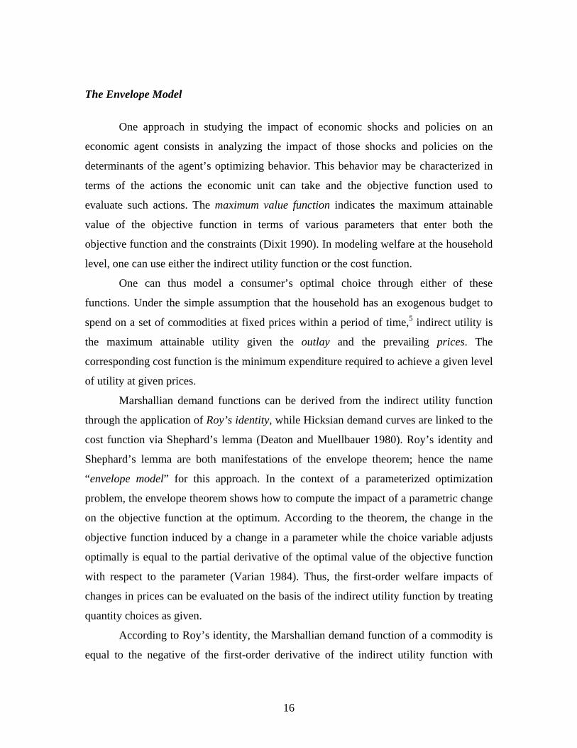
The Envelope Model

One approach in studying the impact of economic shocks and policies on an

economic agent consists in analyzing the impact of those shocks and policies on the

determinants of the agent’s optimizing behavior. This behavior may be characterized in

terms of the actions the economic unit can take and the objective function used to

evaluate such actions. The maximum value function indicates the maximum attainable

value of the objective function in terms of various parameters that enter both the

objective function and the constraints (Dixit 1990). In modeling welfare at the household

level, one can use either the indirect utility function or the cost function.

One can thus model a consumer’s optimal choice through either of these

functions. Under the simple assumption that the household has an exogenous budget to

spend on a set of commodities at fixed prices within a period of time,5 indirect utility is

the maximum attainable utility given the outlay and the prevailing prices. The

corresponding cost function is the minimum expenditure required to achieve a given level

of utility at given prices.

Marshallian demand functions can be derived from the indirect utility function

through the application of Roy’s identity, while Hicksian demand curves are linked to the

cost function via Shephard’s lemma (Deaton and Muellbauer 1980). Roy’s identity and

Shephard’s lemma are both manifestations of the envelope theorem; hence the name

“envelope model” for this approach. In the context of a parameterized optimization

problem, the envelope theorem shows how to compute the impact of a parametric change

on the objective function at the optimum. According to the theorem, the change in the

objective function induced by a change in a parameter while the choice variable adjusts

optimally is equal to the partial derivative of the optimal value of the objective function

with respect to the parameter (Varian 1984). Thus, the first-order welfare impacts of

changes in prices can be evaluated on the basis of the indirect utility function by treating

quantity choices as given.

According to Roy’s identity, the Marshallian demand function of a commodity is

equal to the negative of the first-order derivative of the indirect utility function with

17

respect to the commodity price, divided by the marginal utility of income. The marginal

utility of income is the first-order derivative of the indirect utility function with respect to

income. By Shephard’s lemma, the Hicksian demand function is equal to the first-order

derivative of the cost function with respect to the relevant commodity price.

These are the key results that allow one to trace the welfare implications of any

policy that affects commodity prices and household budgets in a way that also accounts

for heterogeneity among households by using household survey data. Within this simple

framework, heterogeneity stems from differences in demand patterns, other

sociodemographic characteristics of households, and the fact that households may face

different prices for the same commodity.

The envelope approach to policy impact analysis has some limitations because

one can only capture the static effects of the policy reform. Furthermore, the fact that the

envelope theorem is valid only in the neighborhood of the initial optimum makes the

method inappropriate for the study of large price changes or in situations in which the

household is out of equilibrium due to restrictions such as rationing. As noted by Chen

and Ravallion (2004), these cases require an estimation of complete demand and supply

systems. Chen and Ravallion also note that such an estimation is hampered by the general

lack of household-level data on prices and wages.

In the context of the envelope approach, a household is assumed to have

preferences among consumption goods and work effort. Thus, the arguments of the utility

function include both the quantities of the commodities consumed and the labor supply

by activity (including the household’s own productive activities). The budget to be spent

on consumption goods is equal to the wage income, plus the profits from household

enterprises. One can see that, on the assumption that a household will optimize behavior

in both production and consumption, the indirect utility of the household is a function of

the supply prices of the goods the household is selling on the market, the demand prices

of the consumption and intermediate goods, and the wage rates in various activities.

18

Box 4: Unit Record Approach: The Envelope Model Gainers and Losers in Trade Reform in Morocco

In a background paper for the poverty assessment for the Kingdom of Morocco, Ravallion and Lokshin (2004) use the envelope approach to identify the gainers and losers in agricultural trade reforms. The government imposed high tariffs (100 percent) on cereal imports to create incentives for domestic cereal production. The elimination of the high tariffs would reduce domestic cereal prices and therefore hurt net cereal producers at least in the short run. On the other hand, consumers would benefit from lower cereal prices. The identification of winners and losers based on a representative sample of 5,000 households focuses along two dimensions: (1) the position on the distribution of consumption and (2) non-income characteristics (for example, geographic residence, sector of employment).Based on these dimensions, the authors decompose changes in inequality into a vertical component and a horizontal component. The impact of the reforms is considered “vertical” (that is, between income levels) if the initial income level predicts perfectly the gainers and losers in the reforms. In the case of no systematic link between reform impacts and income, there is a “horizontal” element reflecting the fact that impacts vary among people at the same level of initial income. This variation is likely due to non-income characteristics (observable and non-observable). Four policy options are considered: (1) a 10 percent cut in the tariff rate, (2) a 30 percent cut, (3) a 50 percent cut, and (4) a complete elimination of tariffs. (Summary results are presented below.) Ravallion and Lokshin (2004) find that the overall impact of the complete liberalization of the cereal trade on household mean consumption and inequality is very small. However, the impacts vary greatly by household type and region with different income sources and patterns of consumptions. A decomposition of the overall change in inequality as measured by the mean logarithmic deviation (identified as the “impact on inequality” in the table) shows that all the impact on inequality is horizontal rather than vertical.

Gainers and Losers in Four Trade Reform Scenarios

Baseline Policy 1 (10%) Policy 2 (30%) Policy 3 (50%) Policy 4 (100%)National Poverty rate (%) 19.61 20.01 20.33 21.04 22.13 Mean log deviation 0.2850 0.2892 0.290 0.2914 0.2917 Gini index 0.385 0.387 0.389 0.391 0.395 Per capita gain 0 6.519 −23.967 −54.816 −133.81 Production gain 0 −32.078 −69.012 −106.308 −201.017 Consumption gain 0 38.598 45.046 51.492 67.207

Policy 2:

Partial de-protection (30%) Policy 4:

Full de-protection (100%) Impact on inequality: Baseline (0.2850) 0.289 0.292 Vertical component 58% −20% Horizontal component 42% 120%

Source: Ravallion and Lokshin 2004. Policy reforms will generally have implications for the domestic structure of

prices and wages and thus for household welfare. In order to analyze the first-order

19

welfare impacts associated with changes in commodity and factor prices, one can apply

the envelope theorem to the extended indirect utility function. This leads to an expression

of each household’s welfare gain or loss as a weighted sum of proportionate changes in

prices and wages. The weights are relevant income or expenditure levels. For instance,

the proportionate change in the selling price of a commodity is weighted by the

corresponding initial revenue. The change in the demand price is weighted by the initial

expenditure. The change in a wage is weighted by earnings from external (to the

household) labor supply.

In order to explain the heterogeneity of estimated welfare impacts further, one can

assume that the indirect utility profit functions vary with the observed household

characteristics (Chen and Ravallion 2004). It is important to distinguish characteristics

that affect preferences on consumption (for example, the number of children, the stage in

the life cycle, or education) from those affecting outputs from household production

activities (for example, land ownership).

In this extended interpretation of the maximum value model, the net gain from the

price induced by trade reform depends on a household’s consumption, labor supply, and

production activities. In turn, these variables depend on prices and household

characteristics such as: (1) the age of the household head, (2) educational and

demographic characteristics, and (3) land as a fixed factor of production. One can then

use regression analysis to attempt to isolate covariates that might help in the design of a

social-protection policy response to changes in household welfare induced by shocks or

policy reforms. One obvious advantage of linking policy impacts to household

characteristics is the possibility of identifying types of households that are particularly

vulnerable on the basis of their consumption or production behavior. This information is

useful in designing targeted compensatory programs.

The Household Income and Occupational Choice Model

What are the basic determinants of economic welfare distribution at the household

level? Bourguignon and Ferreira (2005) note three groups of factors and propose a

simulation framework whereby the process of household income generation is described

20

in terms of these factors. The configuration of the distribution of income at a given point

in time thus depends on (1) the distribution of factor endowments and sociodemographic

characteristics among the population, (2) the returns to these assets and characteristics,

and (3) the behavior of socioeconomic agents with respect to resource allocation subject

to prevailing institutional constraints. This behavior is reflected in labor-market

participation and occupational choice, consumption patterns, or fertility choices.

Based on this view, the household-income-generation process can be described

parametrically by a set of four equations: (1) an occupation equation, (2) a wage

equation, (3) a self-employment income equation, and (4) an equation for the

computation of household per capita income. The occupational equation, which is based

on a multinomial logit model, describes how household members of working age allocate

their time among wage work, self-employment, and nonmarket activities. The allocation

of the workforce across activities depends on observed characteristics specific to the

individual and the household to which he or she belongs. The allocation also depends on

a set of unobserved variables represented by random variables that are assumed to follow

the law of extreme values and to be identically and independently distributed across

individuals and activities. Given the discrete choice model underlying the allocation of

the labor force, the occupation equation determines the likelihood that a working age

member of a household will be a wage earner, self-employed, or a non-earner. This

likelihood depends on individual characteristics such as education, age, and experience. It

is also a function of household characteristics such as education of the household head,

household size, the dependency ratio, and the place of residence.

The wage equation follows the Mincerian specification whereby the logarithm of

earnings in a given occupation is a linear function of individual characteristics and

random variables that are assumed to follow the standard normal distribution and to be

distributed identically and independently across individuals and occupations. Self-

employment income is similarly modeled. The wage and self-employment equations are

estimated on the basis only of individuals and households with nonzero earnings or self-

employment income. There is thus a need to correct for selection bias.

One approach is to use Heckman’s two-stage estimator. Given the previous three

equations of the model, the last equation of the model computes the per capita household

21

income in two steps. First, total household income is obtained from the aggregation,

across individuals and activities, of earnings and self-employment income, with unearned

income. Second, total household income is divided by household size.

In order to avoid the difficulties associated with the joint estimation of the

participation and earnings equations for each household member, the model is estimated

in reduced form. Thus, results should never be regarded as corresponding to a structural

model, and no causal inference is implied. Bourguignon and Ferreira (2005) explain that

the parameters generated by these equations are merely descriptions of conditional

distributions based on the chosen functional forms.

The model can be used to analyze changes in household income distribution in a

manner analogous to the Oaxaca-Blinder decomposition of changes in mean income

(Bourguignon and Ferreira 2005). Within the Oaxaca-Blinder framework, the income of

an individual is viewed as a linear function of her observed characteristics, say,

endowments, and some unobserved characteristics represented by a random variable. The

linear coefficients are interpreted as rates of return to individual endowments or the

prices of the services from these endowments. If the unobserved characteristics are

distributed independently of the endowments, then one can use ordinary least squares to

estimate the rates of return. If we also assume that the expected value of the residual term

is equal to zero, then the change in mean earnings can be expressed as the sum of two

effects: (1) the endowment effect (associated with a change in the mean endowment at

constant prices) and (2) the price effect (associated with a change in prices at constant

mean endowments).

The interpretation of the above decomposition within the household-income-

generation model generalizes the counterfactual simulation techniques from the single

earnings equation model to a system of multiple nonlinear equations that is meant to

represent mechanisms of household income generation; hence the name “generalized

Oaxaca-Blinder decomposition.” The approach entails simulating counterfactual

distributions, changing market and household behavior one aspect at a time (ceteris

paribus), and noting the effect of each change on the distribution of economic welfare.

Three major effects may thus be identified: (1) endowment effects, (2) price effects, and

(3) occupational effects.

22

Box 5: Unit Record Approach: Household Income and Occupational Choice Model A Microsimulation Study on Côte d’Ivoire

Between 1978 and 1993, Côte d’Ivoire experienced a sharp deterioration in its terms of trade and a significant increase in its external debt. The average annual per capita growth of GDP became negative. Following the 1994 devaluation of the CFA franc and a series of structural reforms supported by both the World Bank and the International Monetary Fund, growth recovered, mainly in the export sector, agro-industry, manufacturing, and energy. Grimm (2004) studied the inequality and poverty implications of macroeconomic adjustment in Côte d’Ivoire. The study focuses on the effects of three phenomena on income distribution: changes in returns to labor, changes in occupational choice, and sociodemographic changes. The analysis is based on the 1993 and 1998 household surveys. Monthly wage and profit functions are estimated in terms of these changes and unobservable effects (reflecting unobservable individual and household characteristics). Income for different sources is aggregated at the household level for 1993 and 1998. The study concludes that income-inequality patterns were different across regions, but poverty trends were similar. In the case of Abidjan, the observed reduction in inequality and poverty is linked to a boost in employment in the formal wage sector and an increase in returns to observable determinants of wage earnings. Rural areas also experienced a strong growth in household income and a significant reduction in poverty. However, these developments were accompanied by a rise in inequality. The negative income growth in Abidjan and the positive income growth in the rural sector were both connected with increasing inequality. Moreover, while within-region inequality increased, between-region inequality declined. For example, while within-inequality increased from 44 percent to 54 by 1998, between-region inequality decreased from 7 percent to 3 percent at the national level by 1998 (see table below).

Decomposition by Microsimulation of the Change in the Distribution

1992/3 1998 National Gini dGini E(0) Gini dGini E(0) Initial values 0.494 0.512 0.508 0.563 Within-group inequality 0.441 0.537 Between-group inequality 0.071 0.026 Observed change 0.014 0.014 Price observables 0.483 −0.011 0.497 0.540 −0.032 0.630 Returns to schooling 0.471 −0.023 0.473 0.547 −0.039 0.640 Returns to experience 0.476 −0.017 0.486 0.512 −0.004 0.573 Ivorian/non-Ivorian wage differential 0.495 0.001 0.515 0.508 0.000 0.562 Regional differential 0.484 −0.010 0.496 0.511 −0.003 0.574 Returns to land 0.489 −0.005 0.506 0.500 0.008 0.550 Residual variance 0.498 0.004 0.525 0.482 0.026 0.515 Total price effects – −0.007 – – −0.006 – Occupational choice 0.496 0.003 0.505 0.515 −0.007 0.557 Price and occupational choice −0.005 −0.014 Population structure effect 0.019 0.028

Source: Grimm 2004. Note: E(0) is the mean logarithmic deviation.

23

3. Embedding Distributional Mechanisms within a General Equilibrium Model The distributional models reviewed in section 2 above have only a limited

application to the analysis of the impacts of macroeconomic shocks and policies on

poverty and income distribution. This limitation stems mainly from the fact that these

approaches fail to account fully for various market and household behavioral

adjustments induced by the shocks or policies. This is the basic reason why these

frameworks are interpreted as reduced-form models. The reliability of their predictions

depends on the reliability of the assumptions made about the impact of macroeconomic

shocks and policies on the key exogenous variables. General equilibrium models can be

used to introduce more structure in the analysis.

In this section, we first review the logic of general equilibrium modeling. We then

examine two ways of modeling distributional mechanisms based on two key sources:

Dervis, de Melo, and Robinson (1982) and Decaluwé and others (1999).

3.1. The Logic of General Equilibrium Modeling What is a General Equilibrium Model? A general equilibrium model is a logical representation of a socioeconomic

system wherein the behavior of all participants is compatible. The key modeling issues

thus entail the following: (1) the identification of the participants, (2) the specification of

individual behavior, (3) the mode of interaction among socioeconomic agents, and (4) the

characterization of compatibility.

The basic Walrasian framework serves as a template for most applied general

equilibrium models. There are two basic categories of agents: consumers and producers,

which are also referred to as households and firms. The behavior of each economic agent

is supposed to conform to the optimization principle according to which the agent

attempts to implement the best feasible action. Thus, modeling optimizing behavior

entails the specification of (1) actions that an economic unit can undertake, (2) the

constraints it faces, and (3) the objective function used to evaluate such actions (Varian

1984). Within this framework, each household buys the best bundle of commodities it

24

can afford. The objective guiding household choice is therefore utility maximization, and

the constraints are expressed in terms of budget constraints. Choices by a firm are

characterized by profit maximization subject to technological and market constraints.

Households and firms are supposed to interact through a network of perfectly

competitive markets. Market interaction is a mode of social coordination through a

mutual adjustment among participants based on quid pro quo (Lindblom 2001).6 Market

participants are buyers and sellers whose supply and demand behavior is an observable

consequence of the optimization assumption. In this setting, behavioral compatibility is

described in terms of market equilibrium. General equilibrium is achieved by an

incentive configuration (as represented through relative prices) such that, for each

market, the amount of demand is equal to the amount supplied. Alternatively, we can say

that, when the economic system is in a state of general equilibrium, no feasible change in

individual behavior is worthwhile, and no desirable change is feasible.

Comparative statics entails a comparison of the equilibrium states associated with

changes in the socioeconomic environment. Such changes may be induced by shocks or

policy reforms. The comparison of equilibrium states can be framed within social

evaluation. The evaluation has two perspectives: individual and social. If we focus on

individual objectives, then Pareto efficiency implies that no participant can be made

better off without making some other participant worse off. A poverty-focused criterion

would say that less poverty is preferable to more.

Empirical Implementation For policy analysis, we need to move from a conceptual framework to a

computable model. Applied general equilibrium models are commonly represented by

systems of equations. These equations fall into the following basic categories:

(1) demand equations from the optimizing behavior of consumers, (2) supply equations

from the optimizing behavior of firms, (3) income equations describing the income of

each agent based on prevailing prices and the quantities exchanged on goods and factors

markets, and (4) equilibrium conditions for all markets. All supply and demand equations

are homogeneous of degree zero. If we multiply all commodity and factor prices by a

constant factor k, the equilibrium supply and demand will not change. Thus, the model is

25

money neutral and can determine only relative prices. This creates the need to normalize

the price system by fixing a numéraire price. The model also satisfies Walras’ Law.

Accordingly, if all economic agents satisfy their budget constraints and all but one of the

markets are in equilibrium, then the last market must automatically be in equilibrium

(Dinwiddy and Teal 1988).

The choice of the functional forms determines the set of structural parameters that

must be estimated in order to make the model computable. The necessary data usually

come in the form of a social accounting matrix (SAM). The matrix reflects the circular

flow of economic activity for the chosen year. It provides an analytically integrated data

set that reflects various aspects of the economy, such as production, consumption, trade,

accumulation, and income distribution. A SAM is a square matrix, the dimension of

which is determined by the institutional setting underlying the economy under

consideration. Each account is represented by a combination of one row and one column

with the same label. Each entry represents a payment to a row account by a column

account. Thus, all receipts into an account are read along the corresponding row, while

payments by the same account are recorded in the corresponding column. In accordance

with the principles of double-entry bookkeeping, the whole construct is subject to a

consistency restriction that makes the column sums equal to the corresponding row sums.

This restriction also means that the SAM obeys Walras’ Law in the sense that, for an n-

dimensional matrix, if the (n-1) accounts balance, so must the last one. Table 2 shows the

structure of a SAM for a model of an open economy.

Table 2. Structure of a SAM for an Open Economy Activity Commodity Factor Household Government Investment World Total

Activity domestic sales export

subsidies exports total sales

Commodity intermediate consumption household

consumption government consumption investment total demand

Factor GDP at factor cost GDP at factor

cost

Household GDP at factor cost transfers foreign

remittances household income

Government indirect taxes tariffs income tax government

revenue

Savings household savings

government savings foreign

savings total savings

World imports total imports

Total production cost total supply GDP at

factor costtotal household expenditure

government expenditure total investment total foreign

exchange

26

For the purpose of analyzing the impact of macroeconomic shocks and policies on

poverty and income distribution, it is important to understand how shocks and policies

affect key macroeconomic balances before considering how the repercussions are

transmitted to households. In general, the macroeconomic properties of a static general

equilibrium model of a real economy such as the one described here depend on the

closure rule chosen. Such a rule refers to the equilibrating mechanisms governing

product and factor markets, as well as the following three basic macro-balances: the

balance of trade, the government budget balance, and the savings-investment balance.

The inevitable inclusion of these macro-balances in the basic Walrasian framework

requires the specification of a corresponding flow equilibrium condition for which a

closure rule has to be stated (Robinson and Löfgren 2005).

Robinson (2003) discusses four possible closures for this class of models. Two of

these assume the full employment of factors of production, while the other two do not.

Assuming that output is a function of two factors of production (capital and labor), there

are 10 potential closure variables: the GDP deflator, the wage rate, the exchange rate,

investment demand, the trade balance, labor supply, the government consumption of

goods and services, capital, the savings rate, and the income tax rate. Closure rules differ

on the basis of which three (the number of macro-balances in the model) of these 10

variables are made endogenous, while all the rest are exogenous.

The first full-employment closure, also known as neoclassical, considers the wage

rate, the exchange rate, and investment demand as endogenous variables. The second

full-employment closure considers the wage rate, the exchange rate, and the balance of

trade as endogenous. Closure rules that assume unemployment are known as Keynesian.

The first rule makes the GDP deflator, the exchange rate, and labor supply endogenous.

For the second rule, the endogenous variables are the GDP deflator, the trade balance,

and labor supply. It is worth noting that the GDP deflator is a numéraire price in the full

employment case, while the wage rate plays that role in the Keynesian case.

A further examination of the neoclassical rule illustrates the types of analytical

restrictions that such rules place on a general equilibrium model for the purpose of

macroeconomic analysis. This rule makes the current account balance7 exogenous, along

with savings rates and government expenditure. Given that the current account balance is

27

related to the functioning of the asset market, making it exogenous means that the

corresponding flow of funds must be added or subtracted from the savings-investment

account (in the SAM). Equivalently, the budget constraint of at least one agent includes

an exogenous net asset change (Robinson and Löfgren 2005). This closure rule leaves

unexplained the decision of households to save at fixed rates and the allocation by

households of savings across different assets.

With respect to the government account, it is commonly assumed that government

expenditure (both consumption and transfers) is fixed in real terms and that government

revenue depends on fixed tax rates. The government deficit or surplus is computed

residually and added to the savings-investment account without any consideration of the

specific financial mechanisms involved.

The above discussion clearly shows that a general equilibrium model based on

this closure will certainly be useful in tackling the medium- to long-term structural

implications of a shock or a policy that works through individual markets, provided it is

sufficiently disaggregated to account for policy-relevant sectors. The model, however,

would have a limited ability to deal with flow-of-funds issues related to the determination

of aggregate savings, the savings-investment balance, and the allocation of investment

across the production sector. This requires the addition of financial mechanisms to the

general equilibrium model.

Robinson and Tyson (1984) offer an illustration with an example of terms-of-

trade shock and the interdependence between structural issues that are essentially

microeconomic in nature and aggregate flow-of-funds issues that are basically

macroeconomic. They also suggest a framework for analyzing this interdependence and

its implications for policy tradeoffs and effectiveness. The basic idea is to link a proper

macroeconomic model to a Walrasian general equilibrium model through variables that

are endogenous in one, but exogenous in the other. For instance, a macro-model may

treat the price level and various macroeconomic aggregates such as employment,

investment and consumption as endogenous. These variables may then be specified as

exogenous in the general equilibrium model. However, the closure rules for macro-

balances and factor markets must be designed in such a way that the general equilibrium

model behaves in a manner that is consistent with the outcome of the macro-model.

28

3.2. Modeling Distributional Mechanisms Dervis, de Melo, and Robinson (1982) note that policy makers might be interested

in how income is distributed among the following: (1) factors of production,

(2) institutions, (3) socioeconomic groups, (4) households, and (5) individuals.

Distribution to factors of production is known as functional distribution, while

distribution to individuals is called size distribution. The choice of the Walrasian

framework with a neoclassical closure focuses analysis on the microeconomic

determinants of income distribution based on relative factor intensities in production and

the interaction between supply and demand and employment.

A sufficiently disaggregated SAM provides a data framework for mappings

among various types of distributions of income. Referring back to table 2, we note that

the functional distribution of income is given by the intersection of the factor-row and the

activity-column. Depending on data availability, this functional distribution can be

disaggregated by sector of production (agriculture, industry, and services) and by labor

categories if the labor market is segmented. When factors of production are further

disaggregated so that labor is differentiated by skill, education, or sector of employment

and capital by type, sector, or region, we get what Löfgren, Robinson, and El-Said (2003)

call the extended functional distribution of income.

GDP at market prices that includes indirect taxes is distributed among various

institutions such as households, enterprises, and government.8 Government revenue from

all taxes is spent on export subsidies, government consumption, and transfers to

households. The residual is put in the capital account. This framework does not explain

various flows of funds related to the activities of the central bank such as money creation

or credit and interest rate policies. Therefore, it would be difficult to analyze the

distributional implications of these macroeconomic policies within this model. Both the

functional and institutional distributions classify flows of funds according to the

functional (factor employment) and institutional structure of the economy.

The household account in the SAM actually stands for all the people in the

economy and may in fact cover all nongovernmental institutions, including enterprises.

Thus, the distributions by socioeconomic groups, households, and individuals are various

29

representations of the distribution of income within this account (Dervis, de Melo, and

Robinson 1982). The classification of individuals or households by socioeconomic group

is dictated by policy issues and data availability. One simple scheme differentiates

groups by type and source of income. Given an exhaustive and mutually exclusive

partition of the entire population into socioeconomic groups, it is possible to derive the

overall size distribution of income as a weighted sum of within-group density functions.

Using the log variance as an indicator of relative inequality, overall inequality can be

decomposed into within-group and between-group components. Thus, ceteris paribus, an

increase in inequality in any one group or an increase in the distance between one group’s

average income and the overall mean income will increase overall inequality. Given the

fact that the overall size distribution is derived empirically, one can compute any desired

measure of inequality or poverty (given a poverty line). When it comes to simulating the

inequality implications of shocks and policies, only between-group inequality can be

generated endogenously by this framework through changes in group means. This is

because within-group distributions are exogenous.

The fact that the overall distribution of income is derived numerically as a

weighted sum of individual group distributions makes it possible to allow the functional

form to vary from group to group. The lognormal distribution that has often been used in

this context is known to provide a poor approximation of the distribution at the upper

extreme. One could use the Pareto distribution for high-income groups. Employing a

different function for every within-group distribution increases the ability of the model to

capture the heterogeneity of socioeconomic groups. Decaluwé and others (1999) use the

Beta distribution to this effect. This function is fully characterized by the minimum

income, the maximum income, and two shape parameters defining the skewness of the

distribution. In a model of an archetypical developing country, these authors allow the

four characteristic parameters of the Beta distribution to vary across six socioeconomic

groups: (1) landless rural households, (2) rural smallholders, (3) big landlords, (4) urban

households with poorly educated heads, (5) urban households with highly educated

heads, and (6) capitalists.9 Instead of aggregating group distributions into an overall

distribution, the authors compute, for each group, poverty measures of the Foster–Greer–

Thorbecke family. Overall poverty can then be inferred as a weighted sum of within-

30

group poverty whereby the weights are given by population shares. Decaluwé and others

(1999) allow the nominal poverty line to be determined within the model. The value of

the reference basket of goods is adjusted on the basis of equilibrium prices computed by

the model.

Box 6: Computable General Equilibrium Model The Impact of Trade Policies on Income Distribution in a Planning Model for Colombia

De Melo and Robinson (1980) use a multisector static CGE model to simulate the effect of trade on both the functional and the size distributions of income in Columbia. The model focuses on the real economy and tries to capture the economic dualism and structural rigidities characteristic of Columbia. Seven broad socioeconomic groups are considered: small farmers, marginal laborers, industrial laborers, service-sector laborers, agricultural capitalists, industrial capitalists, and service-sector capitalists. These groups are assumed to have different consumption patterns, and the size distribution within each group is represented by a lognormal distribution. The CGE model endogenously determines various incomes, consumption and investment, and trade flows. Based on these results, the distribution of income to socioeconomic groups and the overall size distribution by individuals are estimated. The study investigates the impact of three alternative trade regimes on the distribution of income in Colombia and compares them with the free trade alternative (FT): an inward-looking strategy with a 50 percent tariff on manufacturing sectors (ILS), an outward-looking strategy with a 50 percent subsidy on agricultural and manufacturing exports (OLS), and a direct-subsidy strategy that provides a 50 percent value-added subsidy to manufacturing sectors (DDS). The simulation results are presented below. The study finds that the domestic price system in Columbia is insulated from changes in world market prices. Furthermore, outward-looking trade policies with increased primary exports are likely to have an adverse impact on the distribution of income in the medium term compared to inward-looking policies. This conclusion depends on the structure of exports and imports. Colombian exports are concentrated in primary goods; imports are mostly manufactured goods,and the country is self-sufficient in food production. In such a case, an open trade strategy is likely to decrease the purchasing power and real incomes of most socioeconomic groups.

Income Distribution Measures for a Model of Colombia

FT ILS OLS DSS Net mean income Rural income 5.55 5.60 5.53 4.88 Unskilled urban 11.82 11.89 11.79 12 Skilled labor 25.72 26.44 25.46 30.39 Rural capitalist 37.47 36.75 38.62 33.55 Manufacturing capitalist 160.85 166.50 159.02 204.82 Service capitalist 67.68 66.30 66.14 63.12 Economy-wide mean income 19.00 19.09 19.00 19.47 Aggregate measures Mean income (top 10%) 98.09 98.36 98.44 104.86 Mean income (bottom 10%) 2.90 2.93 2.88 2.69 Rural poverty 58.51 58.05 59.53 62.92 Urban poverty 41.48 41.95 40.47 37.08 Total poverty 29.90 29.40 30.30 32.10 Gini coefficient 0.581 0.580 0.583 0.601

Source: de Melo and Robinson 1980.

31

The basic idea underlying the approach discussed here involves linking an

extended functional distribution to a size distribution of income. Various socioeconomic

groups are considered as representative households. Thus, we call this approach the

Extended representative household (ERH) approach to distinguish it from the standard

representative household (RH) approach, which limits the analysis of the distributional

impact of shocks and policies to their effects on representative socioeconomic groups.

There is one other way of implementing the ERH approach (discussed in Agénor, Chen,

and Grimm 2004). The treatment of the size distribution in this case is analogous to the

approach underlying PovStat. Indeed, it is assumed that, following a shock or the

implementation of a policy, per capita consumption and disposable income for a

household change at the same rate as the one predicted by the general equilibrium model

for the socioeconomic group to which the household belongs.10 Thus, the size distribution

is represented directly by relevant unit records from a household survey. Following a

shock or the implementation of a policy, a new distribution of income and consumption is

generated by applying the predicted rates of change to the initial data. New measures of

poverty and inequality can thus be computed and compared to baseline values.

This approach can only predict changes in between-group inequality because the

income and consumption of all the households belonging to a same socioeconomic group

are scaled (up or down) by the same factor. Another limitation of this approach noted by

the authors is due to the fact that it does not account for changes in the structure of

employment. Therefore, they propose an extension of the approach based on a

reweighing procedure that reassigns population weights to households in a manner that is

consistent with predicted changes in employment structure.

4. Linking a Macroeconomic Framework to a Model of Income Distribution To be sure, both the standard RH and the ERH approaches reveal the basic

principles involved in linking a macroeconomic model to a representation of the

distribution of economic welfare across individuals or households. In this section, we

focus on some specific models (tools) that have been built more or less around these

principles. We first describe the 123PRSP model, a three-layer and parsimonious

framework designed to link macroeconomic policies to poverty outcomes via a two-

32

sector general equilibrium model of an open economy.

We then consider two implementations of the PAMS framework. The first

interpretation of this framework uses the ERH approach based on unit records to simulate

the poverty impact of macroeconomic shocks and policies analyzed within a macro-

consistency model such as the Revised Minimum Standard Model Extended (RMSM-X).

The second interpretation is a reduced-form of the first whereby a CGE model is linked

recursively (in a top-down fashion) to a poverty module built upon a parameterization of

the Lorenz curve à la POVCAL.

We then review a different macro-micro simulation model whereby the

macroeconomy is represented by an IS-LM model.

Finally, we describe briefly the IMMPA framework, which links a dynamic CGE

model including a financial sector to a distributional module that is analogous to PovStat.

Given our distributional concerns, we must judge these models ultimately on the

basis of how well they use the wealth of available information (from national accounts

and household surveys) to explain the interdependence among sectors and institutions

and the heterogeneity of actors. Naturally, in a particular environment, additional criteria

come into play, such as the skills required of the analyst to implement a given approach.

4.1. The 123PRSP Model The 123PRSP model is based on the idea that the impact on poverty of

macroeconomic shocks and policies is transmitted through two basic channels. The first

channel involves distributional-neutral changes in the average income, while the second

is the change in the sectoral pattern of growth induced by changes in relative prices (for

example, changes in the real exchange rate). The overall impact is thus equal to the pure

growth impact, plus the distributional impact.

This idea is implemented within a three-layer model. The macro-layer has three

components: (1) a financial programming model, (2) a trivariate vector autoregressive

(VAR) model, and (3) a medium-term growth model based on cross-country regression

analysis. The meso- (or intermediate) layer is represented by a two-sector general

equilibrium model of an open economy. Finally, the micro-layer relies on the envelope

theorem to model the distribution of welfare across households.

33

The Financial Programming Module Generally speaking, financial programming is the process of designing a

consistent set of macroeconomic policies whereby instruments (for example, domestic

credit) are set in such a way that a target variable (official reserves, for example) follows

a desired trajectory. In the context of policy reform programs supported by the

International Monetary Fund, this approach is used to set monetary and fiscal policies

aimed at restraining aggregate demand and adjusting relative prices. Financial

programming can be described in terms of the underlying accounting framework that

imposes consistency upon data and any prediction based on assumed behavioral

relationships or projection rules.11 The approach emphasizes the monetary dimension of

the balance of payments and relates the monetary and fiscal accounts to the balance of

payments.

The economy is divided into four institutional sectors: (1) the private sector,

(2) the public (government) sector, (3) the foreign sector or the rest of the world, and

(4) the domestic banking sector. Each sector in the economy is represented by a budget

that constrains its behavior, and all variables are measured in nominal local currency.

Within this framework, financial transactions are distinguished from those arising from

the production or acquisition of goods and services (also known as income/expenditure

transactions). It is assumed that the private sector owns all factors of production. The

private sector gets nominal income from the sale of current output. This income is used to

pay taxes to the government, purchase goods for consumption, and make investments.

Any disposable income after expenditure is used to accumulate financial assets or

liabilities in the form of money, foreign assets, and borrowing from the banking system.

The public sector collects taxes from the private sector and uses the proceeds for

consumption. Any surplus or deficit is accounted for by the accumulation of financial

assets or liabilities in the form of foreign assets and net borrowing from the banking

system. The foreign sector gets revenues from the sale of imports to the domestic

economy. It spends on domestic exports. In the case of a current account deficit, the

revenues of the foreign sector exceed its expenditures. The foreign sector can buy back

its liabilities from the domestic private and public sectors and acquires reserves from the

34

domestic banking system. The financial sector functions as a financial intermediary

among various actors. It obtains assets in the form of international reserves and claims on

domestic actors and issues its own liabilities in the form of money to the private sector.

These budget constraints are not independent; they represent an overall resource

constraint on the economy. This resource constraint can be expressed as follows: the

difference between gross national disposable income and domestic absorption is equal to

the current account balance.12 The linkages among these sectoral accounts imply that a

deficit in any sector must be financed by savings in other sectors. For the whole

economy, excess spending is possible only if financing is available from the rest of the

world. The relationship between excess absorption and the current account balance shows

that an improvement in the latter may be achieved through an increase in the country’s

output or a reduction in absorption. Furthermore, the sum of the current account balance

and net capital inflows is equal to the change in net official reserves. This identity links

excess absorption (over income) to two financing sources: capital inflows to the

nonbanking sector and official international reserves. This clearly shows that the current

account balance acts as a resource constraint on the whole economy (IMF 1987).

The basic structure of the financial programming model can be understood by

focusing on the case of a small open economy with a fixed exchange rate, which is

known as the Polak model (Agénor 2004a; Polak 1998; IMF 1987). In this context, the

money supply is viewed as an endogenous variable that depends on changes in the

balance of payments.

The core model contains four relationships. The first relationship is an accounting

identity based on the balance sheet of the banking system.13 Accordingly, the change in

the money supply (a liability for the banking system) equals the sum of the change in net

official reserves and the change in net domestic credit (that is, the sum of changes in the

foreign and domestic assets held by the banking system). The second relationship defines

the change in the nominal demand for money as the change in the nominal income times

the inverse of the income velocity of money assumed constant over time. The third

relationship defines flow equilibrium in the money market. The last relationship restates

the balance-of-payments identity as follows: the change in official reserves is equal to

exports, minus imports, plus the change in net capital inflows to the nonbanking system.

35

Exports are assumed to be exogenous, while imports are computed as national income

times a constant marginal propensity to import.

The design of a financial program involves an iterative process based on the

following five steps (IMF 1987). (1) Set the target for the change in the official reserves.

(2) Use the last relationship (the balance-of-payments identity) to compute residually a

value for imports consistent with the reserve target and the assumed level of the

exogenous variables (exports and the change in net capital flows to the nonbanking

sector). (3) Project nominal income and use the projection, along with the assumed values

for the income velocity of money and the marginal propensity to import, in order to

obtain the demands for money and imports. (4) Given a forecast of the money demand

(equal to the money supply in equilibrium) and the target for official reserves, use the

balance-sheet identity of the banking system (first equation) to infer the change in

domestic credit compatible with the target for official reserves and the desired increase in

nominal money balances. (5) Check for consistency by comparing the projected imports

with the residual value computed from the balance-of-payments identity in step 2. If the

two values are equal, stop the process; if not, make further adjustments to the underlying

assumptions and repeat the process until consistency is achieved.

Monetary and fiscal policy can be linked through the financial programming

framework by distinguishing the expansion of credit to the private sector from that to the

public sector (IMF 1987). Thus, the total change in the domestic assets of the banking

system appearing in the balance-sheet identity must now include two components: (1) the

change in domestic credit to the government and (2) the change in domestic credit to the

private sector. Similarly, the total change in foreign capital inflows to the nonbanking

sector has two components, public and private. Finally, a relationship must be added to

reflect the fact that the government can finance its budget deficit through net borrowing

either from abroad or from the domestic banking system.

The Growth Module The growth module has two components. The first, a trivariate VAR model

designed to capture the short-run growth impact of a shock such as an improvement or a

deterioration in the terms of trade, or the short-run growth impact of a policy reform such

36

as a change in government expenditure. The VAR model is a useful tool for analyzing

interrelationships among different time-series. In this framework, all variables are

endogenous because of the assumption that the time path of each variable affects and is

affected by current and past realizations of the other variables. A VAR model may be

characterized by the number of variables (time-series) and the longest lag length (Enders

1995). Thus, a first-order bivariate VAR would involve two variables and a lag length of

at most one. The random disturbances in the VAR framework are known as innovations

or shocks. A shock in one variable not only affects that variable directly, but is also

transmitted to all the other variables depending on the lag structure of the model. A VAR

can be written as a vector moving-average of the shocks, from which one can derive

impulse response functions. An impulse response function represents the behavior of

time-series in response to various shocks. The 123PRSP framework includes the

following three variables: the growth rate, the real exchange rate, and either the terms of

trade or government expenditure. The parameter estimates from impulse response

functions are interpreted as short-run growth elasticities.

The second component of the growth module is a cross-country regression model

(Easterly 2001) designed to capture the impact of macroeconomic policies on long-run

growth. The model involves three groups of independent variables. The first group

includes policy determinants of growth: (1) a black market premium, (2) a measure of

financial development (M2/GDP),14 (3) inflation, (4) the real exchange rate,

(5) secondary education enrollment, and (6) telephone lines per 1,000 individuals (a

proxy for infrastructure stock). The second group of variables captures the impact of

shocks such as (1) the terms of trade as a percentage of GDP, (2) the interest on external

debt as a percentage of GDP, and (3) Organisation for Economic Co-operation and

Development trading partner growth. Finally, variables measuring initial conditions

include: (1) initial income, (2) intercept, (3) a dummy variable for the 1980s, and (4) a

dummy variable for the 1990s.

The Two-Sector General Equilibrium Model

The meso-layer of the 123PRSP is represented by a two-sector general

equilibrium model of a small open economy. The model is a generalization of the Salter-

37

Swan framework, which provides a foundation for the study of the impact of

macroeconomic imbalances and adjustment policies on the real sector of the economy.

This single-country model (as opposed to a multi-country trade model) represents a

significant improvement on both the standard neoclassical trade model and the Salter-

Swan model. The neoclassical model often leads to implausible empirical results because

of two basic assumptions. The first assumption states that all goods are tradable, while

the second implies perfect substitutability between foreign and domestic goods. These

two assumptions imply the law of one price, according to which the domestic prices of

tradable goods and services are determined by the world market.

The Salter-Swan framework makes an important distinction between tradable and

nontradable goods and services. Nontradables are goods and services the prices of which

are determined by supply and demand conditions within domestic markets. Prices for

tradable goods are determined by the world market. The fact that a good is nontradable

may be due to its nature (such as public services or construction) or to prohibitive

transport costs that keep the good off the world market. Thus, some policy changes can

cause some goods to switch categories. Furthermore, the country under consideration is

assumed to be small with respect to international trade and therefore faces a perfectly

elastic excess supply from the rest of the world. In other words, it cannot affect the terms

at which it is trading with the rest of the world. Exportable and importable goods can

therefore be aggregated into a single class of good, tradables, using world prices as

weights. The model still maintains the neoclassical assumption that domestic and foreign

goods are perfect substitutes in consumption and focuses on the effects of external shocks

on the real exchange rate, which ultimately directs resource allocation within the

economy.

The extension of this framework implemented within the 123PRSP drops the

aggregation and perfect substitution assumptions and explicitly adds government,

savings, and investment.15 These extensions allow the inclusion of policy instruments

such as taxes, as well as the consideration of macroeconomic effects. We now briefly

describe this extension (see Devarajan, Lewis, and Robinson 1990 for a more detailed

presentation).

The small country assumption is maintained; thus, the country cannot affect its

38

terms of trade with the rest of the world. There are two sectors of production. The first

produces exports, and the second produces all other final goods, which are referred to as

domestic (home) goods. Real GDP is an aggregation of exports and domestic goods

based on a constant elasticity of transformation (CET) function.16 The supply of exports

relative to domestic goods is obtained by maximizing GDP, subject to the technical

transformability constraint (above) and sales opportunities at home and abroad.

Consumption is expressed in terms of a composite good that is an aggregation of

home goods and imports based on a constant elasticity of substitution function. The

demand for imports and for domestic goods is derived by minimizing the cost of the

composite good, subject to a substitutability constraint represented by the elasticity of

substitution function. The representative household is assumed to save a constant fraction

of its disposable income. Gross income is the sum of GDP, transfers from the public

sector, and remittances from abroad.

The domestic prices of exports and imports are calculated from world prices, the

exchange rate, and all applicable taxes. The GDP deflator is a weighted average of the

domestic price of exports and that of home goods. The weights are the shares of each

commodity in GDP. Similarly, the aggregate price of the composite consumption good is

a weighted average of the domestic price of imports and home goods.

Two types of equilibrium conditions are explicitly stated. The first group concerns

commodity market equilibrium: (1) the supply of home goods equals the demand, and

(2) the supply of the composite good equals the demand, which includes private

consumption, investment, and government consumption (assumed to be fixed in real

terms). The other group of conditions pertains to macroeconomic balances: (1) the

current account balance is fixed; (2) total savings (the sum of private, public, and foreign

savings) equals investment, and (3) government revenue from direct and indirect taxes is

accounted for by government consumption, transfers, and savings. There are also implicit

equilibrium conditions associated with the use of the CET production-possibility frontier.

This assumption is a cover for the operation of factor markets (labor and capital). Indeed,

it is equivalent to assuming full employment in a single labor market within the economy.

In this static model, capital is assumed to be fixed and sector specific. Thus, there is an

equilibrium wage rate associated with each equilibrium price for home goods. Returns to

39

capital in each sector can be computed residually from the value of output.

The financial programming model and the growth module trace the

macroeconomic implications of shocks and policies. In particular, these two sub-modules

produce information on the evolution of GDP that is consistent with the underlying

macroeconomic framework over the relevant horizon. The 1-2-3 model then takes this

information and computes the structural implications induced by a change in relative

prices. This is a key link in the chain of transmission from macroeconomic events to

poverty. Based on the distinction between tradable and nontradable commodities, the real

exchange rate is defined as the price of tradables relative to nontradable goods. An

increase in the domestic prices relative to world prices is known as an appreciation of the

real exchange rate, while a decrease marks a depreciation. Real appreciation of the

exchange rate, for instance, shifts incentives in favor of domestic goods relative to

exports. The final outcome depends on the structural characteristics of the economy as

revealed by the elasticity of transformation and substitution.

The Micro-Layer

The purpose of the micro-layer is to translate the solution of the 1-2-3 general

equilibrium model into changes in household welfare. For any macroeconomic event

worked out within the macroeconomic framework, the general equilibrium model

computes the corresponding changes in income (wages and profit) by sector (tradable and

nontradable) and the changes in commodity prices (imports and home goods). The

construction of the household module follows the envelope approach (discussed earlier).

Here, the indirect utility is a function of the wage rate, sectoral profits, and commodity

prices. These are the linkage variables between the meso- and the micro-layers. Thus, the

first-order approximation of the welfare impact of a macro-shock at the household level

is equal to the sum of three components: (1) the initial level of labor income times the

relative change in the wage rate, (2) the change in profit income, and (3) the sum over

commodities of the product of the negative of the initial consumption and the relative

change in the commodity price.17

For the empirical implementation, distributions of income and expenditure by

40

deciles are derived from available household survey data. There are three income

sources: wages, profits from the home goods sector, and profits from the exports sector.

Consumption expenditure is divided among imports and domestic goods. Heterogeneity

among households is thus reflected by differences in the sources of incomes and in the

patterns of consumption. This helps capture the differential impacts among households of

shocks and policies.

Consider, for instance, a cut in public expenditure that falls mainly on nontradable

goods. If there is sufficient structural flexibility, the induced fall in the price of

nontradables will lead to a real depreciation in the exchange rate. The production of

tradable goods will increase, while that of nontradables will decline. The welfare impact

at the household level will depend on whether a household is a net seller or a net buyer of

tradable goods. Net sellers would gain, while net buyers would lose. Once these

differential impacts are computed, standard techniques can be used to derive the desired

poverty and inequality measures. However, it is important to keep in mind that, even

when abundant and relevant household-level data are available, the ability of a modular

framework such as 123PRSP to account for heterogeneity is constrained by the degree of

disaggregation at the meso-level. By unifying the labor market and dividing the economy

into only two sectors, the 123PRSP model achieves a great deal of transparency at a

significant cost in terms of heterogeneity.18

41

Box 7: The 123PRSP Model: Distributional Effects of Macro-Policies and Shocks in Zambia

Devarajan and Go (2003) employ the 123PRSP model to examine the distributional impact of macroeconomic shocks and policies in Zambia. Zambia is a landlocked economy that depends heavily on mineral exports (particularly copper). This renders the country very vulnerable to external price shocks. Over the 2001–3period, two risk factors threatened macroeconomic stability in Zambia. The first shock stemmedfrom expenditure pressures associated with the presidential election in late 2001, and the second from the decline in the world price of copper (the major export for the economy) induced by a slowdown in world demand. One scenario assumes a 15 percent increase in government consumption in 2001 followed by another 10 percent increase in 2002. Assuming that foreign borrowing is kept at a constant fraction of GDP with respect to the base case and that investment adjusts to the available total savings, model simulations show a small increase in GDP the first year that disappears the following year. The first-round multiplier effects of a rise in government consumption are offset by the crowding-out effect of high fiscal deficits in subsequent periods. The results also show small increases in consumption and household incomes. Another simulation combines the expenditure shock with a decline in the copper price by 20 percent the first year, 15 percent the second year, and 10 percent the third year. The results(see table below) show that these shocks would lead to a significant drop in GDP growth of about 0.5 percent the first year, 1.4 percent the second year, and 1.3 percent the third year. Relative to the base case, household income falls about 2 percent the first year, cumulating to about 6 percent the last year. Even though all household groups are affected negatively, the results show that the poorest are the hardest hit.

Impact of Shocks in Government Expenditures and Copper Prices (Percentage deviation from the reference run, unless otherwise stated)

2001 2002 2003 Real GDP (% +/-) Expenditure shock 0.6 –0.1 0.1 Expenditure +TOT –0.5 –1.4 –1.3 Real exchange rate of exports(depreciation>0) Expenditure shock 0 0 0 Expenditure +TOT 7.9 7.9 7.9 Household income (real) Expenditure +TOT Decile 1 (poorest) –4.6 –8.0 –9.8 Decile 2 –4.2 –7.4 –9.2 Decile 3 –4.0 –7.0 –8.8 Decile 4 –3.6 –6.4 –8.2 Decile 5 –3.4 –6.1 –7.8 Decile 6 –2.6 –5.0 –6.6 Decile 7 –2.4 –4.7 –6.3 Decile 8 –2.7 –5.1 –6.7 Decile 9 –2.5 –4.8 –6.4 Decile 10 (richest) –1.7 –3.7 –5.3 Total –2.1 –4.4 –5.8

Source: Devarajan and Go 2003.

42

4.2. The PAMS Framework

PAMS is a simple simulation framework analogous to the 123PRSP to the extent that it is

designed to help trace sequentially, in a top-down fashion, the poverty and distributional

implications of macroeconomic shocks or policies. The original implementation of this

framework (PAMS I) has three layers. The macroeconomic layer is represented by a

standard macro-consistency model such as the World Bank’s RMSM-X.

The second layer, which represents the meso-level of analysis, is based on the

idea that each household in the economy gets its means of livelihood both from the

government (net public transfers) and from the market. The micro-layer deals with

household-level information organized on the basis of policy relevant characteristics in a

way that allows easy linkages with the meso-framework. Unit record data are used in a

manner analogous to PovStat. The second generation of the framework is a reduced-form

application that combines the macro- and meso-layers into a general equilibrium model

and employs a parameterization of the Lorenz curve for poverty simulation.

In this section, we discuss the macroeconomic module within the RMSM-X

framework. Then we provide a brief description of the meso-module and the poverty

simulator. We close the section with a brief description of the essential features of the

reduced-form version, which links a CGE model to a parameterized Lorenz curve.

The RMSM-X Module

In essence, the RMSM-X framework may be viewed as an extension of a financial

programming model that includes a growth model specified along the lines of the Harrod-

Domar model.19 In the basic formulation, there are four economic agents or sectors in the

economy: (1) the central government, (2) the monetary system, (3) the private sector, and

(4) the rest of the world (or the foreign sector). The underlying macroeconomic

accounting framework is the same as the one described in the section on financial

programming. It obeys the principles of flow-of-funds accounting: (1) a source of funds

for one sector represents a use of funds by another sector, and (2) for each sector, the

total amount of funds from all sources must equal the total disposition for all uses.

43

The structure of the model is characterized by (1) the budget constraints facing

each sector and the overall economy, (2) market equilibrium conditions for goods and

asset markets, and (3) behavioral and projection rules linking some variables to others.

Consider in particular an economy with the four sectors and three assets above, including

money, domestic lending by the banking system, and foreign debt.20 A basic RMSM-X

model could then be specified along the following lines. The growth equation establishes

a relationship between the growth of real output, investment, and the incremental capital

output ratio (ICOR). A standard assumption is that the ICOR is constant over time, which

implies a proportional relationship between growth and investment.21 Next, one includes

two equations describing changes in nominal output and changes in the overall price

index. The change in the overall price index can be defined as a weighted average of

changes in the index of domestic prices and changes in the exchange rate.

On the financial side of the economy, one would add the following relationships

from the financial programming framework. A money supply equation would be derived

from the balance sheet of the banking system. The equilibrium condition in the domestic

lending market states that a change in domestic credit is the sum of credit to the private

sector and credit to the public sector. Credit to the private sector could be expressed as a

function of the change in nominal GDP. The change in official reserves is derived from

the balance-of-payments identity. In this identity, exports are exogenous and computed

on the basis of a simple projection rule. Imports can be computed as a function of real

income and the real exchange rate (Agénor 2004a). The flow of foreign debt is given by

the equilibrium condition on the foreign asset market, which states that the total flow is

equal to the sum of private and public flows. As before, the demand for money is a

function of the velocity parameter and nominal income. Flow equilibrium prevails in the

money market.

The budget constraints of both the public and private sectors can be written in a

reduced form that shows the accumulation of assets and liabilities associated with a

surplus or deficit. In addition, the budget constraint of the private sector can be combined

with the assumption that private consumption is a linear function of disposable income so

as to compute investment (Agénor 2004a).

Adding up the four budget constraints in the model gives the fundamental national

44

income identity. The model therefore contains eight core equations represented by the

four budget constraints, the derived national income identity, and the three flow

equilibrium conditions in asset markets (money, domestic credit, and foreign debt). These

core equations are not mathematically independent due to the relationship between the

sectoral budgets and the overall resource constraint. The system thus obeys Walras’ Law

and can be solved on the basis of only seven of the core equations. The solution of the

remaining equation can be inferred from that of the other seven. However, the solution

procedure depends on the closures chosen. There are three common closure rules (World

Bank 1995). In the case of public closure, one seeks values of government consumption

and borrowing from both the monetary system and abroad that are consistent with

projected growth, inflation, and other variables. In the private closure, one seeks a

solution in terms of private consumption and borrowing. With respect to the policy

closure, one is interested in the likely impact of alternative macroeconomic programs on

target variables such as growth and inflation.

The policy closure seems more appropriate when the module is used to study the

impact of macroeconomic policies on poverty and the distribution of income. In this

context, one could solve the system recursively as follows (World Bank 1995). Step one:

identify and fix all foreign borrowing available to the country; then compute imports

residually from the balance of payments. Step two: use the value of imports derived from

step one in the national income identity to solve for private investment.22 Step three:

compute the value of the second target variable, the current price, from the money market

equilibrium and the money demand equation.23 Step four: derive total domestic credit

residually from the money supply equation. Step five: given the change in government

credit, compute private credit residually from the equilibrium condition of the domestic

credit market.

The Meso-Module

The main element of this component is the labor and wage-income module, which

reconfigures the productive sector of the economy into a number of sectors equal to the

number of socioeconomic groups. This effectively leads to a segmented labor market in

45

the module. This segmentation is achieved as follows. First, the module divides the

economy into two basic components, rural and urban. Then, within each component, we

distinguish the formal sector from the informal sector. Within each of these sectors,

subsectors producing tradables are distinguished from those producing nontradables.

GDP, which is determined at the macro-level, is an important linkage variable and

must also be broken down according to the above categories. Here again, it will be

necessary to determine residually the production of certain sectors (for example, the

urban informal sector and the rural subsistence sector) in order to maintain overall

consistency. The simplest way to model the rural economy is to represent its output as a

constant elasticity function of rural labor. Within the urban economy, the production of

the public sector is exogenous. Assuming that all private investment in the economy

occurs within the formal sector, the output in that sector can be computed on the basis of

an appropriate incremental capital output ratio. In such a case, the growth rate of output

in the urban formal economy would stand in a fixed-coefficient relationship with the ratio

of investment to output. For the sake of consistency, the output of the informal

nontradable sector is determined residually.

Labor supply is seen as largely driven by demographic considerations and semi-

exogenous migrations of labor and skill categories. Labor demand is broken down by

socioeconomic categories, skill levels, and location – rural and urban – and is viewed as

dependent on sectoral demand (output growth), as well as real wages. Hence, the new

module determines wage income broken down by socioeconomic categories, skill levels,

and location (rural and urban). Even though each sector in the reconfigured economy may

employ both skilled and unskilled labor, the module relies on a simplifying assumption

according to which each sector employs only one kind of labor. Thus, there is no

substitution between types of labor in the production process except for semi-exogenous

migration based on the Harris-Todaro process.

The excess of the total income generated in the economy with respect to the total

wage bill distributed to all labor categories represents the profits that are distributed to a

representative class of rentiers. The current version of the tool does not track down

financial assets and returns on these assets. However, the interest revenue can

conceivably be redistributed from the macro-framework to various socioeconomic groups

46

according to some rule. Average tax and transfer rates are used in order to compute the

disposable income for each socioeconomic group. It is the percentage change in this

disposable income that is transmitted to the poverty simulator in order to simulate the

impact of shocks and policies on poverty and between-group inequality.

The Poverty Simulator

The poverty simulator in this version of PAMS (PAMS I) is analogous to PovStat.

Intra-group distributions are represented by unit records pertaining to each

socioeconomic group. In order to compute the impact of a macroeconomic shock or a

policy on the welfare of a given household, the per capita income or expenditure of the

household is multiplied by the induced growth rate of the disposable income of the

representative group to which the household belongs. This growth rate is jointly

determined by the macro- and the meso-layers.

As with any of the frameworks examined here, there are structural and, possibly,

data constraints that can limit the reliability of the framework in predicting the poverty

and distributional impact of macroeconomic shocks and policies. In the particular case of

PAMS I, there is a data constraint stemming from the fact that most household surveys

provide some information at the household level, such as expenditure and self-

employment income, while other information, such as labor income and employment

status, is given at the individual level. Choosing the household as the unit of analysis

means that individual-level data must be aggregated up to the household level.

Socioeconomic groups are thus created on the basis of the characteristics of heads of

household. This obviously leads to results that are coarser than results based on relevant

individual-level data.

In addition, the poverty simulator is bound to inherit the strengths and weaknesses

of the top layers. It is well known, for instance, that the basic RMSM-X is a simple

macroeconomic accounting framework and shows no behavioral relationships in the

economic sense. Also, the use of a labor demand function that is defined by sector and

skill level is equivalent to assuming a homogenous labor factor with different, sector-

specific remuneration.

47

Operational Support

PAMS I has seen battle in support of the design of Poverty Reduction Support

Credits and the Poverty Assessment for Burkina Faso. Specifically, the framework was

used to simulate the poverty implications of negative shocks to the cotton sector, as well

as the impact of some patterns of growth. Assuming a permanent 20 percent decline in

the price of cotton starting in 2004, the simulations reveal an increase of about

1.5 percentage points above the baseline. Naturally, cotton farmers (18 percent of the

population) are the most affected. This impact would be exacerbated if it were

accompanied by drop of 20 percent in output.

In the context of the analysis of the implications of different growth patterns, the

simulation framework was used to study the impact of shocks to the agriculture sector

outside cotton. A 20 percent increase in the output of the primary sector could lead to a

3 percentage point decline in poverty. One set of simulations concerns the implications of

a pattern of growth whereby the overall growth rate remains unchanged, while the

primary sector grows at a rate 2 percent higher than the baseline, along with a lower

growth rate for the tertiary sector. In this case, poverty falls by 1 percent up to 2007 and

4 percentage points by 2015.

Reduced-Form Implementation

The purpose of the meso-layer in the original PAMS is to model an extended

functional distribution of the income generated by the upper-layer macroeconomic model

based on the selected socioeconomic groups. In practice, several iterations are required in

order to calibrate this module to available data. If a disaggregated SAM is available that

is compatible with the selected socioeconomic groups, then it might be easier to compress

the macro- and meso-layers into a general equilibrium model. As far as the poverty

simulator is concerned, we note that multiplying each observation (expenditure or

income) in the unit record representation of a distribution by a scalar implies that the

mean of the distribution is multiplied by the same scalar. Given that the within-group

group distribution remains constant from one state to another, one might as well construct

48

the poverty simulator on the basis of group means and Lorenz functions estimated from

the available household data.

Box 8: PAMS II A Reduced-Form Application of PAMS to Indonesia

Essama-Nssah (2004) explains the implementation of a reduced-form version of PAMS using Indonesian data. The poverty outcomes of policies are analyzed by linking recursively the CGE model to a poverty simulator built upon a parameterization of the Lorenz curve. The aggregate formulation employs private consumption as the key linking variable, while the multisector interpretation relies on real disposable income. The poverty simulator of PAMS II is used to study the poverty implications of (1) terms-of-trade shocks, (2) changes in the balance of trade, and (3) changes in income tax or indirect taxes. The reduced-form version developed for Indonesia (known as INDOPAMS) represents a significant improvement both computationally and in the modeling of the links between poverty and distributional outcomes and the macroeconomy. Furthermore, the version collapses the macro- and meso-modules of the original framework into a simple CGE model. This approach allows one to endogenize to some extent the growth process via factor accumulation. In the application, the key linkage variable is the mean of the distribution of income or expenditure, the changes of which are determined by the economy-wide model. These changes are then fed into the Lorenz framework to predict the corresponding changes in poverty. In accordance with the ERH approach that underlies it, PAMS II assumes constant intra-group inequality. Thus, it can only predict changes in between-group inequality. Various scenarios were simulated to examine the impact on poverty and inequality indicators. The table below shows, for instance, the poverty implications of an export boom in the form of a 20 percent increase in the world price of exports. It is clear that the extent of poverty reduction depends crucially on the structure of the economy as represented by the elasticities of output transformation and import substitution. The higher these elasticities, the greater the extent of poverty reduction.

Poverty Implications of an Improvement in the Terms of Trade

Elasticity of Output Transformation

Import Substitution Elasticity

Headcount (Base) Headcount (20%) Poverty Gap (Base) Poverty Gap (20%)

–0.20 0.20 0.161 0.145 0.023 0.019 –0.50 0.50 0.161 0.133 0.023 0.017 –0.75 1.26 0.161 0.128 0.023 0.016 –2.00 2.00 0.161 0.126 0.023 0.015 –5.00 5.00 0.161 0.121 0.023 0.014

Source: Essama-Nssah 2004.

This approach increases computational efficiency in a simulation environment.

Thus, within the reduced-form version of PAMS (PAMS II) that runs in EViews (version

4.1 or later), poverty and distributional outcomes of shocks and policies are derived by

linking recursively an appropriately disaggregated CGE model with a poverty and

inequality simulator built upon a parameterization of the Lorenz curve. The approach

underlying PAMS II is analogous to the ERH approach described earlier. The main

difference with other implementations of this approach stems from the fact that, in the

49

PAMS framework, the within-group size distribution of income is derived from the

assumed Lorenz distribution. Many other applications assume functional forms for the

density function characterizing the within-group distribution.

4.3. A Macro-Micro Simulation Model for Brazil

In the context of this review, a macro-micro simulation model stands for any

simulation framework that links in some fashion a representation of the macroeconomy to

a model of the size distribution of income. In this fundamental sense, the 123PRSP

model, PAMS, and even the ERH framework are members of the family of macro-micro

simulation models. Two approaches commonly followed in the literature are to combine

a CGE model either with an envelope model of welfare distribution or with an income

and occupational model. The first approach is analogous to the way 123PRSP links a

two-sector CGE model to the corresponding household module. Given this analogy and

the fact that we have already reviewed the structure of CGE models and income-

occupational models, we focus here only an approach followed by Ferreira and others

(2004) in a study of the distributional impacts of macroeconomic shocks in Brazil. They

link a IS-LM model to a model of income and occupational choice. We consider only the

macroeconomic model and the linkage variables.

The IS-LM Model The basic IS-LM model is considered an expression of the Keynesian approach to

macroeconomics24 and is based on a key assumption: aggregate demand determines the

equilibrium level of output. The model provides a framework for the study of the

interaction between the real and the financial sides of the economy. This interaction is

governed by two key variables: the real economy determines the level of income, which

affects the demand for money (a financial variable), and the financial sector determines

the interest rate, which affects investment in the real economy.

The Brazilian model reviewed here is a neo-Keynesian extension of the above

basic framework; it has three basic components. The real economy block of the model

determines the aggregate demand, production, and factor demand components. The

50

second block models the determination of the price level and the wage rate. Finally, the

interest rate is determined in the financial block of the model. The basic transmission

mechanism between the real and the financial sides of the economy relies on the

specification of real private consumption and investment as functions of the interest rate.

Private consumption is also a function of disposable income and the general price index.

The model includes a disaggregated representation of the balance of payments.

In order to improve the ability of the model to handle the agent heterogeneity

observed in the household survey, supply is divided into six sectors: (1) urban tradable

formal, (2) urban nontradable formal, (3) urban nontradable informal, (4) rural tradable

formal, (5) rural nontradable formal, and (6) rural nontradable informal. Production in

each of these sectors is assumed to be an elasticity of substitution function of capital and

a composite labor input with skilled and unskilled components. Labor demand by skill

level (low, intermediate, and high) is determined by profit maximization.

Linkage Variables The solution of the model affords the linkage variables needed for impact analysis

with the microsimulation module. In particular, it produces 18 wage rates (for three skill

levels in six sectors), and 21 occupation rates (six employment levels and one value for

unemployment for six sectors). Another set of linkage variables includes changes in

output prices in the six sectors. The authors use an algorithm to ensure consistency

between the macroeconomic solution and the predictions of the microsimulation model.

4.4. The IMMPA Framework The IMMPA is a dynamic framework designed around some key characteristics

of low-income countries. It focuses on issues relating to labor-market segmentation,

informal activities, credit market imperfections, and the composition of public

expenditure. The macro- and meso-parts of the economy are represented by a financial

CGE model with seven distinct blocks: (1) production and employment, (2) the demand

side of the economy, (3) the price system, (4) external trade, (5) income formation,

(6) the financial sector, and (7) the public sector. The specification of each of these

blocks follows well-known principles in general equilibrium modeling. We will therefore

51

focus the presentation here on some key distinctive features of the IMMPA.

We note at the outset that this framework is richer than any of those described

above. It allows the analyst to consider the segmentation of the labor market induced by

legislation or wage-setting practices, along with the role of informal employment in the

transmission of the impact of shocks and policies to the poor. For highly indebted

countries, one can analyze the effects of foreign debt on private incentives to invest. The

integration of the real and financial sides of the economy in the context of credit market

imperfections allows a realistic consideration of stabilization and structural policy issues.

Finally, by distinguishing the components of public expenditure on infrastructure, health,

and education, the framework permits a disaggregated impact analysis. While this

structural richness is desirable for a proper accounting of heterogeneity, it may also prove

to be a severe constraint to implementation in a data-poor environment.

The Labor Market With respect to the modeling of the labor market, the IMMPA framework

emphasizes the idea that the structure of labor plays a crucial role in the transmission of

the impact of shocks and policies to economic activity, employment, and relative prices.

This is especially important because, generally speaking, labor supply is a major source

of income for the poor in many countries. The framework distinguishes between the rural

and the urban sectors of the economy. The urban labor market has two components: the

formal and the informal segments. Wages are assumed to be fully flexible in the informal

economy. In the formal sector, labor is heterogeneous and comprises a skilled element

and an unskilled element. Wages for skilled workers in the private sector are fixed on the

basis of efficiency wage considerations. The government determines the wages for public

sector employees and unskilled workers in the formal private sector.

It is assumed that unskilled workers can work in the rural and urban sectors, while

skilled workers are restricted to the urban sector. The labor force in rural areas grows at

an exogenous rate equal to the population growth rate, minus the net migration to urban

areas. According to the Harris Todaro model, migration is governed by the differential

between the expected wage in the rural sector and the one prevailing in the urban sector.

52

The Financial Sector The modeling of the financial sector is based on features of an archetypical poor

economy with a limited number of financial assets. This component of the framework

seeks to determine the structure of the portfolio held by households, the demand for

credit by firms, and the behavior of commercial banks. Savings can be held only in the

form of money or bank deposits at home and abroad. Financial intermediation is

dominated by commercial banks. A key assumption states that firms are unable to issue

tradable claims on their assets or future output. The framework also tries to capture the

impact of interest rates on capital flows and the structure of agent portfolios, the real

balance effects on expenditure, and the linkages between bank credit and the supply side

of the economy through the demand for working capital by firms. In particular, the bank

lending rate is incorporated in the effective price of labor faced by firms that must

finance their working capital needs prior to the sale of output. This is one of the crucial

ways in which the real and financial sides of the economy interact.

Public Expenditure The IMMPA framework is designed to account for the channels through which

various components of public investment affect the economy. In particular, the stock of

public capital in infrastructure (roads, power plants, and railroads) is assumed to have a

direct effect on the level of production in the private sector and, hence, on the marginal

productivity of primary factors employed in that sector.

Public expenditure on education consists of spending on such items as school

buildings and other infrastructure and is assumed to have an impact if it assists unskilled

workers to acquire skills. Similarly, public assets such as hospitals and health centers

affect individual health outcomes.

Distributional Analysis For the purpose of distributional analysis, the IMMPA framework considers six

categories of households: (1) workers in the rural traded sector, (2) workers in the rural

nontraded sector, (3) unskilled workers in the urban informal sector, (4) unskilled

workers in the urban formal sector, (5) skilled workers in the urban formal sector, and

53

Box 9: The IMMPA Model: Adjustment Policies and the Poor in Brazil Brazil has made significant progress in controlling inflation and achieving stabilization since the Real Plan of 1994. Despite the 1999 currency crisis, which put pressure on the exchange rate and led to the adoption of a flexible exchange rate regime, inflation remained low. This stabilization was achieved through a prudent fiscal policy and active management of short-term interest rates by the central bank. Agénor and others (forthcoming) provide an interpretation of the IMMPA framework to analyze the impact of adjustment policies on poverty and income distribution in Brazil. The interpretation involves extensions to the prototype framework in order to capture important characteristics specific to the Brazilian economy. In particular, the Brazilian model allows for open unskilled urban unemployment, a distinction between product wage and consumption wage in the determination of skilled worker wages, the possibility of congestion effects linked to the use of public services in urban areas, and bond financing of public sector deficits, while excluding borrowing from the central bank. The poverty and distributional implications of a 10 percent increase in the interest rate are presented in the table below. In the short run, the poverty headcount index increases only slightly in both rural and urban areas. However, in the long run, the increase in the official interest rate would cause the headcount index to rise by 2 percent in urban areas and 3 percent in rural areas. The households engaged in urban informal activities are the hardest hit group. Poverty among this group increases by about 5 percent. Income inequality increases as well. Overall, higher interest rates (a tight monetary policy) will lower inflation, but at the expense of greater poverty and income inequality.

Brazil Simulation Results: Impact of a 10 Percentage Point Increase in the Interest Rate

Poverty and Distributional Indicators, Consumption Based

Period 1 Period 2 Period 3 Period 8 Period 9 Period 10

Poverty headcount Rural households –0.1 0.1 0.2 1.5 2.6 3.0 Urban households –0.6 0.0 –0.1 1.0 1.5 2.2

Informal –0.1 0.0 0.1 2.5 3.3 4.9 Formal unskilled –1.8 –0.1 0.0 0.5 0.8 0.9 Formal skilled –0.1 –0.1 –0.4 0.0 0.2 0.3 Capitalists and rentiers 0.5 0.5 0.0 –1.0 –1.0 –0.7

Economy –0.5 0.0 0.0 1.1 1.7 2.3 Distributional indicators Gini coefficient –2.3 –0.3 0.0 3.8 4.6 5.3 Theil index –1.2 –0.3 –0.1 3.7 4.9 6.2

Source: Agénor and others, forthcoming.

(6) capitalists. The macroeconomic model is linked to unit record data in a way that is

analogous to impact analysis with PovStat. Following a shock to the model economy, the

macro-model generates real growth rates in per capita consumption and disposable

income for all six household categories and for each year in the simulation horizon (up to

10 years). These growth rates are then used to scale per capita consumption and

disposable income appropriately in each group. New poverty and inequality indicators

(the Foster–Greer–Thorbecke family, the Gini, and the Theil) are computed and

compared to the baseline values. The difference is attributed to the shock. In this dynamic

54

framework, short-term impact corresponds to the first two periods. Medium-term impact

is supposed to occur between periods 3 and 5. Long-term impact is felt beyond period 6.

5. Concluding Remarks This paper reviews some common approaches in modeling the poverty and

distributional impact of macroeconomic shocks and policies, such as terms-of-trade

shocks, fiscal adjustment, monetary policy, and trade liberalization. What is needed in

these situations is a framework that adequately links a macroeconomic model to a model

of the distribution of economic welfare at the individual or household level.

The approaches or specific models reviewed in this paper vary in the ways they

specify the macroeconomy, the distribution of welfare, and the macro-micro linkages.

Models that focus only on income distribution may be viewed as frameworks that keep

the macro-model implicit. They can therefore be used in conjunction with assumptions

about the response of the macroeconomy to shocks and policies. The second approach

involves embedding distributional mechanisms within a general equilibrium framework,

while the third class of models adopts a modular approach in linking poverty and

distributional outcomes to macroeconomic shocks and policies. An emerging approach

known as Top-Down/Bottom-Up or TD/BU (Savard 2005) is worth mentioning. It tries to

account for the feedback effect from the micro-module to the macro and back until

convergence is achieved. Which approach to adopt depends, of course, on the problem at

hand, the data, and other constraints imposed by modeling resources, such as skills.

The reliability of a model designed to predict the poverty and distributional

outcomes of macroeconomic shocks and policies depends on how well the model handles

three fundamentals. The first relates to the heterogeneity of socioeconomic agents in

terms of endowments (assets and personal characteristics) and behavior. The availability

of reliable household data is a key constraint in accounting for such heterogeneity. The

second fundamental concerns the modeling of transmission channels in terms of

institutional arrangements that control social interaction. A realistic representation of

such arrangements allows one to estimate more accurately both the direct and the indirect

effects of shocks and policies. Finally, the macroeconomic model should be designed to

account for the interdependence among policy issues (stabilization, structural and

55

distributional). In a modular approach, the ability of the bottom layer to account for

heterogeneity can be severely constrained by the top layers if they are not disaggregated

in a way that is consistent with the bottom layer. It may therefore be said that the whole

framework is only as “strong” as its “weakest” module.

56

Annex Description of Selected Tools for the Poverty and Social Impact Analysis of

Macroeconomic Shocks and Policies

Source: A User’s Guide to Poverty and Social Impact Analysis

(World Bank 2003)

57

Tool name: Social Accounting Matrices

What is it?

A SAM is a technique related to national income accounting that provides a conceptual basis for examining growth and distributional issues within a single analytical framework. It can be seen as a tool for the organization of information in a single matrix of the interaction between production, income, consumption, and capital accumulation.

What can it be used for? SAMs can be used for some simple policy simulations.

What does it tell you? SAMs can be applied to the analysis of the interrelationships between structural features of an economy and the distribution of income and expenditure among household groups.

Complementary tools: SAMS would complement and be complemented by the use of household surveys to map impacts into distributional changes. Stakeholder analysis can be useful in identifying different groups of interest.

Key elements:

A typical SAM contains entries for productive activities, commodities, factors, institutions, the capital account, and the “rest of the world.” An activity produces (and receives income from) commodities, buys commodities as production inputs, and pays wages to labor, rents to capital, and taxes to the government. Factor income accrues to households as owners of the factors. The SAM can be constructed to distinguish household groups by, for example, sources of income. SAM techniques select some accounts as exogenous and leave the remaining accounts endogenous. In part, this selection can be made on a sound theoretical basis, but it is often arbitrary. For example, if the SAM contains an account for agricultural production and one for transportation, an experiment can be run by imposing some exogenous change (a “shock”) to agriculture, while leaving the transport sector fixed or while allowing the transport sector to adjust endogenously as a result of the shock.

Data/information: The data sources for a SAM come from input-output tables, national income statistics, and a household survey with a labor module.

Time: About three months for a moderately detailed SAM.

Skills: Working with household data sets, strong knowledge of national accounts, and use of Excel and, maybe, the General Algebraic Modeling System (for using dedicated software).

Supporting software:

Excel and dedicated software based on the General Algebraic Modeling System, and Stata, SAS, or Statistical Package for the Social Sciences for working with household data sets. R

equi

rem

ents

Financial cost: US$25,000 when the data are available. This does not include the cost of developing a new household survey.

Limitations:

SAM models have at least two major drawbacks. First, prices are fixed and do not adjust to reflect changes in, say, real activity. As a result, supply is either perfectly elastic (if chosen to be endogenous) and entirely demand driven, or perfectly inelastic, that is, supply is constant. Second, the results of the simulations vary greatly depending on the assumptions made about which accounts are exogenous and which accounts are endogenous.

References and applications:

For an overview of the technique, see Round (2003). Pyatt and Round (1985). Powell and Round (2000). Reinert and Roland-Holst (1997). Sadoulet and de Janvry (1995). Tarp, Roland-Holst, and Rand (2002).

58

Tool name: Computable General Equilibrium Models

What is it?

CGE models are completely-specified models of an economy or a region, including all production activities, factors, and institutions. The models therefore include the modeling of all markets (in which agent decisions are price responsive and markets reconcile supply and demand decisions) and macroeconomic components, such as investment and savings, balance of payments, and government budget.

What can it be used for?

CGEs can be used to analyze the poverty and social impacts of a wide range of policies, including exogenous shocks (exchange rate, international prices, etc.), changes in taxation, subsidies, and public expenditure (including changes in trade policies), and changes in the domestic economic and social structure (including technological changes, asset redistribution, and human capital formation).

What does it tell you?

CGE models are best chosen for policy analysis when the socioeconomic structure, prices, and macroeconomic phenomena all prove important for the analysis. CGEs allow one to take into account all the sectors of the economy, as well as the macroeconomy and, hence, permit the explicit examination of both the direct and the indirect consequences of policies. This is particularly important for those policy reforms that are likely to play a large role in the economy and might have important impacts on other sectors or on the flow of foreign exchange or capital.

Complementary tools: Other tools described here belong to this class of models, with an additional model to take distribution into account: the 123PRSP, IMMPA, and the augmented CGE model with a representative household approach. See the respective tables in this annex.

Key elements:

A CGE can be described by specifying the agents and their behavior, the rules that bring the different markets in equilibrium, and the macroeconomic characteristics. CGEs are based on SAMs (see the table on Social Accounting Matrices) and can be distinguished by the complexity and the level of disaggregation of productive activities, factors, and institutions, including households.

Data/information: CGE models are data intensive. They are constructed from combined national accounts and survey data. These are first compiled into a SAM, which is then used as the foundation of the CGE.

Time:

A few months to a year, depending on the existence of a SAM or of another CGE model built to address a different question. Even these simple CGEs can be complex and time consuming. An alternative is to use a previously constructed CGE. For example, Ianchovichina, Nicita, and Soloaga (2001) use a CGE model constructed by the Global Trade and Analysis Project to examine the impact of the North American Free Trade Agreement on household welfare in Mexico. However, the use of a previously constructed simple CGE can limit the number of policy changes that can be simulated. (In the last example, the model was constructed to examine trade policy and did not cover domestic taxes or public expenditure.)

Skills: Experienced modelers with substantial prior exposure to CGE models are required. Supporting software: Excel, EViews, Gauss.

Req

uire

men

ts

Financial cost: US$25,000–75,000 depending on the existing data.

Limitations:

The results of CGE simulations depend at least partly on the assumptions made in the model, such as the “closure” rules. These ensure that macroeconomic accounts (fiscal, trade, savings-investment) balance. Whether they are fixed exogenously or allowed to balance endogenously, as well as how they balance, can have a significant impact on the outcomes. In addition, the production accounts specified in most available CGEs are too aggregated to identify the impact of policy changes in one component of one account. Many CGEs have at most two agricultural activities, one each for tradable and nontradable crops, or food crops and cash crops.


Dervis, de Melo, and Robinson (1982), Decaluwé and others (1999), and Shoven and Whalley (1992) for summaries of the CGE models used.

Ianchovichina, Nicita, and Soloaga (2001). Global Trade and Analysis Project models at www.gtap.agecon.purdue.edu.

59

Tool name: PovStat

What is it? An Excel-based software program that simulates the changes in poverty and inequality resulting over time from changes in growth in output and employment.

What can it be used for? PovStat may be used to simulate the poverty and inequality impact of policies affecting sector-level output and employment growth rates.


PovStat simulates poverty and inequality measures under alternative growth scenarios. Forecasts of varying levels of complexity may be computed, depending on the availability of reliable data and the extent to which factors influencing poverty levels are incorporated. The simulations vary according to optional projection parameters.

Complementary tools: Other software programs that provide poverty and inequality forecasts include SimSIP Poverty (see the table on SimSIP) and DAD (a software for distributive analysis).

Key elements:

On the basis of household-level data, the software translates differential output and employment growth across sectors into differential growth in the per capita income or consumption of households across those sectors. The tool simulates the impact on poverty of policies affecting output. It does this by using the fact that poverty changes can be decomposed into two parts: a component related to the uniform growth of income and a component due to changes in relative income. The simulations are made under the assumption that the policy analyzed will be distribution neutral, or, conversely, that there is a specific, quantifiable form for the distributional change. Changes in employment distribution are accommodated by reweighing the sample households.

Data/information:

This program requires unit record household-survey data. Also, a poverty line, survey year, and forecast horizon are parameters that must be provided by the user. Macroeconomic variables at the nationally aggregated or sectorally disaggregated level and growth rates of income, employment, and population are also required. In addition, the user can input changes in the CPI and GDP deflator, changes in the relative prices of food and the shares of food in CPI, and changes in the poverty line consumption bundle. This allows one to generate different types of forecasts and optional projection parameters such as employment shifts across sectors. The software can be adapted for grouped data.

Time: One or two days to format the household survey data, collate and check exogenous economic variables, and enter everything into PovStat.

Skills: Familiarity with Excel and appropriate household data-handling software (such as Stata). Also, familiarity with PovCal if synthetic data from a grouped distribution are to be used.

Supporting software: Excel.

Req

uire

men

ts

Financial cost: –

Limitations: PovStat does not capture second-round effects. These may be captured by CGE models.


For an overview of the technique, see Datt and others (2003). Datt and Walker (2002). Software available at www.worldbank.org/psia, “Tools and Methods.”

60

Tool name: SimSIP Poverty

What is it? SimSIP Poverty is a generic Excel-based simulator that allows one to estimate the changes in poverty and inequality over time resulting from changes in output and employment growth.

What can it be used for? This tool may be used to simulate the poverty and inequality impact of policies affecting sector-level output and employment growth.

What does it tell you? It simulates poverty and inequality measures nationally and within sectors (urban and rural, agriculture, manufacturing, and services). It may simulate the impact that various sectoral growth patterns and population shifts between sectors will have on future poverty and inequality.

Complementary tools: Other tools for poverty forecasting include PovStat (see the table on PovStat) and DAD (a software for distributive analysis).

Key elements:

On the basis of existing information on group-level household survey data (typically by deciles or quintiles), the software translates differential output and employment growth across sectors into differential growth in the per capita income or consumption of households across these sectors. The tool simulates the impact on poverty of policies affecting output by using the fact that poverty changes can be decomposed into two parts: a component related to the uniform growth of income and a component due to changes in relative income. The simulations are made under the assumption that the policy analyzed will be distribution neutral or, conversely, that there is a specific, quantifiable form for the distributional change. Changes in employment distribution are accommodated by reweighing the sample households.

Data/information:

SimSIP Poverty uses grouped household data, typically grouped by income; the mean income or consumption by group and the share of these groups are required. In addition, SimSIP Poverty requires macroeconomic data at a nationally aggregated or sectorally disaggregated level. This includes, for example, past or expected growth rates of output, employment, and population by sector. Finally, the population size and growth and a poverty line are necessary for calculating poverty incidence.

Time: One day to gather the data on population shares and mean income or consumption by group, check the credibility of scenarios, and enter the data into the software.

Skills: Familiarity with Excel. Supporting software: Excel.

Req

uire

men

ts

Financial cost: –

Limitations: SimSIP does not capture second-round effects. These may be captured by CGE models.


For an overview of the technique, see Datt and others(2003). Wodon, Ramadas, and van der Mensbrugghe (2003). Ramadas, van der Mensbrugghe, and Wodon (2002). Software available at www.worldbank.org/simsip.

61

Tool name: 123PRSP

What is it? 123PRSP (one country, two sectors, and three goods) is a static CGE model.

What can it be used for? 123PRSP can be used to analyze the impact of macroeconomic policy and external shocks on income distribution, employment, and poverty.


It allows for a forecast of welfare measures and poverty outcomes that is consistent with a set of macroeconomic policies in the context of a very simple general equilibrium model. For a given set of macroeconomic policies, 123PRSP generates a set of wages, sector-specific profits, and relative prices that are mutually consistent. The projected changes in prices, wages, and profits are then inputted into household data on wages, profits, and commodity demand among representative groups or segments of the distribution. In principle, 123PRSP can calculate the policy impact on each household in the sample so as to capture the effect on the entire distribution of income. For a given poverty line, 123PRSP can also compute the effect of different poverty measures.

Complementary tools:

Analysis of impacts on income distribution could be complemented by social impact analysis and institutional analysis, which look at variables that would affect household participation in growth. Scenario analysis, which helps policy makers assess the effects of major discontinuities on economic projections, could complement CGE models operating on a long-time horizon.

Key elements:

123PRSP can be viewed as a middle ground between consistency models such as RMSM-X and more sophisticated approaches such as disaggregated CGE models. The former are simple to estimate and use, but consider the two most important determinants of poverty – economic growth and relative prices – as exogenous. The latter are useful for capturing the poverty impacts of policies, but are too data intensive and difficult to master. One salient feature of 123PRSP is its modular approach; by linking several existing models together, it can make use of individual modules that already exist. Furthermore, if a particular module is not available because of data-related reasons or other reasons, the rest of the framework can be implemented without it.

Data/information:

The 123PRSP model requires national accounts, a SAM, and some basic distributional data or a household survey. The model builds on an existing static aggregate model, such as the International Monetary Fund’s Financial Programming Model (containing a consistent set of national accounts that are linked with fiscal balance of payments and monetary accounts). Macroeconomic policies are then fed into the “get real module” or an alternative country-specific model of long-run growth determination and into a trivariate VAR module of short-run fluctuations. This trivariate module would require historical national account data. Both long-run and short-run projections would then feed into the 1-2-3 model to generate projections on changes in wages, profits, and the prices of the three goods, which in turn are fed into a household data module to capture the effects of macroeconomic policies on poverty.

Time: About three months if a household survey and the macro-model are available.

Skills: Experienced modelers with expertise in financial programming and advanced time-series econometrics. Supporting software: EViews, Excel.

Req

uire

men

ts

Financial cost: Aside from any cost for the development of the macro-model or the household survey, about US$25,000 to set out a new model.

Limitations:

As noted above, 123PRSP adopts several strategic simplifications in order to make the model user-friendly. The disadvantage of adopting this approach is that the causal chain from macroeconomic policies to poverty is in one direction only. In this regard, the model does not capture the feedback effect of changes in the composition of demand (due to shifts in the distribution of income) on macroeconomic balances.


For an overview of the technique, see Devarajan and Go (2003).

.

62

Tool name: Poverty Analysis Macroeconomic Simulator

What is it? PAMS is an econometric model that links a macro-consistency model or macroeconomic framework to a labor-poverty module.

What can it be used for? PAMS can be used to address the impact of macroeconomic policies and exogenous shocks (such as an exogenous rise or fall in output growth or a change in the sectoral composition of output) on individual households.


PAMS can produce historical or counterfactual simulations of (1) alternative growth scenarios with different assumptions for inflation and fiscal and current account balances; these simulations allow tradeoffs within a macro-stabilization program to be tested; (2) different combinations of sectoral growth (agricultural or industrial, tradable or nontradable goods sectors) within a given aggregate GDP growth rate; and (3) tax and budgetary transfer policies.

Complementary tools: Stakeholder analysis can be useful for identifying groups to inform the process of selecting microcategories.

Key elements:

PAMS has three main components. First is a standard aggregate macro-framework that can be taken from any macro-consistency model (for example, RMSM-X, 123) to project GDP, national accounts, the national budget, the balance of payments, price levels, etc., in aggregate consistent accounts. Second is a labor-market model that breaks down labor categories by skill level and economic sectors in which the production total is consistent with that of the macro-framework. Individuals from the household surveys are joined in representative groups of households defined by the labor categories of the heads of household. For each labor category, labor demand depends on sectoral output and real wages. Wage-income levels by economic sector and labor category can thus be determined. In addition, different income tax rates and different levels of budgetary transfers across labor categories can be added to wage income. Third is a model that uses the labor-model results for each labor category to simulate the income growth for each individual inside a group, which is assumed to be a representative group. After projecting individual incomes, PAMS calculates the incidence of poverty and the inter-group inequality.

Data/information: The model requires national accounts with a breakdown by sector, household survey data with income or expenditure data by unit, and a wage and employment breakdown by sector.

Time:

With a macro-model, the time needed to build a PAMS would be about three months: (1) one month to select or extract categories of households from the household survey and match the economic sectors from the macro-model, (2) one month to link the macro-model to the household survey data, and (3) one month to run the macro- and household-module together and adjust.

Skills: Knowledge is required of (1) national-accounts-based macroeconomic models, (2) basic labor-demand models, and (3) the structure of household surveys.

Supporting software: EViews, Excel.

Req

uire

men

ts

Financial cost: US$25,000 when the data are available. This does not include the cost of developing a macro-model or a new household survey.

Limitations: The main limitation is the lack of feedback of the micro-model into the macro-model. References and applications:

For an overview, see Pereira da Silva, Essama-Nssah, and Samaké (2003). Pereira da Silva, Essama-Nssah, and Samaké (2002).

63

Tool name: Integrated Macroeconomic Model for Poverty Analysis

What is it? IMMPA is a dynamic CGE model.

What can it be used for? IMMPA can be used to analyze the impact of macroeconomic policy and external shocks on income distribution, employment, and poverty.


One of the main features of IMMPA is that it integrates the real and financial sides of the economy; in this regard, IMMPA is useful for analyzing both the impact of structural reforms (such as changes in tariffs or the composition of public expenditure) and the effects of short-term stabilization policies (such as a cut in domestic credit or a rise in deposit interest rates). The detailed treatment of the labor market is key for the assessment of the poverty reduction impact of macroeconomic policies. Also, it is useful for drawing the distinction between rural and urban sectors by completing separate projections on output and employment fluctuations for both areas and therefore to study poverty in different geographical areas.

Complementary tools: IMMPA would complement and be complemented by the use of household surveys to map impacts into distributional changes. Stakeholder analysis can be useful for identifying different groups that are of interest.

Key Elements:

The main features that distinguish IMMPA from other CGE models are as follows. First, IMMPA offers a very detailed specification of the labor market, which is the main transmission channel of macroeconomic shocks and adjustment policies to economic activity, employment, and relative prices. The labor-market specification permits a disaggregation at the urban and rural levels and, within each level, in the formal and informal sectors. Second, IMMPA links real and financial sectors through an explicit treatment of the financial system. Third, the model emphasizes the negative effect of external debt on private investment and therefore incorporates the possibility of debt overhang. Finally, IMMPA accounts explicitly for the channels through which various types of public investment outlay affect the economy.

Data/information:

The greatest drawback of any fully specified CGE model is the time and data required to construct it. The model must be constructed from combined national accounts and survey data. These are first compiled into a SAM, which is then used as the foundation for the model. IMMPA, for example, consists of 131 equations, more than 30 exogenous variables, and more than 200 endogenous variables.

Time: The process can take more than a year and rarely less than a few months.

Skills: Experienced modelers with substantial prior exposure to CGE models are required. Supporting software: EViews, Excel.

Req

uire

men

ts

Financial cost: US$75,000 to develop the IMMPA general equilibrium model.

Limitations: CGE simulations depend to a large extent on the assumptions made in the model, especially those that are required to close the model. They are also data intensive and difficult to master, which could limit the usefulness of the model under tight deadlines or capacity constraints.


Agénor, Izquierdo, and Fofack (2003).

64

Tool name: Augmented CGE Model with the Representative Household Approach

What is it? This technique is based on a CGE model with representative households that are linked to a household module.

What can it be used for? RH models can be used to analyze the impact of macroeconomic policy and external shocks on income distribution, employment, and poverty.

What does it tell you? RH models allow for a forecast of welfare measures and poverty outcomes consistent with a set of macroeconomic policies in the context of a general equilibrium model.

Complementary tools: –

Key elements:

The key features of the RH approach are, first, a CGE model that incorporates markets for factors and commodities and their links to the rest of the economy and that generates equilibrium values for employment, wages, and commodity prices, as well as “extended” functional distributions (that is, labor differentiated by skill, education, gender, region, and sector of employment) and, second, a mapping from the extended functional distribution into the “size” distribution (the distribution of income across different households). In this approach, the representative households that appear in the CGE (corresponding to aggregates or averages of groups of households) play a crucial role: the “size” distribution is generated by feeding data on the simulated outcomes for the representative households into a separate module that contains additional information about each household.

Data/information: RH models require a SAM and distributional data describing the representative household groups or, more specifically, a household survey.

Time: Only a few days to generate a base solution if data and skills are available. Between six months and a year to collect data and work with the simulations.

Skills: Experienced modelers with substantial prior exposure to CGE models are required. Supporting software: Excel, EViews, Gauss. R

equi

rem

ents

Financial cost: US$25,000–75,000 depending on the data that exist.

Limitations: In the absence of a CGE model to feed into the RH module, the model is data intensive and difficult to master.


For an overview, see Löfgren, Robinson, and El-Said (2003). Robilliard, Bourguignon, and Robinson (2001) on Indonesia. Coady and Harris (2001) on Mexico. Löfgren, Harris, and Robinson(2002).

65

Notes 1. Our review focuses on models dealing primarily with the income dimension of poverty. The Development Economics Development Prospects Group at the World Bank has established a framework known as MAMS or Maquette for MDG Simulation. This framework allows an economy-wide analysis of shocks and policies on income poverty and a set of Millennium Development Goals (MDGs) related to health, education, and infrastructure (see Löfgren and Diaz-Bonilla 2005). 2. Most economic models of behavior are based on the principle of optimization, according to which each agent attempts to implement the best possible action given her/his objective and the prevailing constraints. The maximum value function is the maximum attainable value of the objective function expressed in terms of the parameters characterizing the environment of the problem (see Dixit 1990). 3. POVCAL is programmed in Fortran 5.0 and uses the parametric specification of the underlying Lorenz curve. Currently, it supports the following specifications: (1) the general quadratic model (Villasenor and Arnold 1984) and (2) the Beta model (Kakwani 1980). 4. The ASCII data file must be in tabular form whereby each row of data corresponds to a record and columns represent the variable for the subgroups. Variables must be organized by order of subgroups. 5. In other terms, the household is facing a linear budget constraint. The institutional underpinning of this assumption consists of efficient markets with negligible transaction costs (Deaton and Muellbauer 1980). 6. According to Lindblom (2001), social coordination aims at minimizing conflict and promoting cooperation viewed as an exchange of help. Lindblom also notes a fundamental distinction between the notions of market and market system. There are markets whenever people frequently pay others to do something. A market system is a collection of markets designed to organize and coordinate social interaction. 7. This is a record of the foreign exchange inflows and outflows associated with trade, with factor and interest payments, and with institutional transfers, including migrant remittances. 8. It is assumed here that indirect taxes are paid at the factory gate. That is why, in the SAM, they appear as a payment by the activity account to the government account. However, such taxes may also be paid out of the commodity account. 9. The parameters can be estimated from household survey data. Alternatively, group density functions can be estimated from relevant parameterized Lorenz curves, as is done in the discussion of the PAMS framework. 10. Agénor, Chen, and Grimm (2004) consider the following categories: (1) rural workers, (2) urban workers in the informal sector, (3) urban unskilled workers in the formal sector, (4) urban skilled workers in the formal sector, and (5) capitalists-rentiers. This does not mean that any policy model should follow the same disaggregation. As mentioned earlier, disaggregation in terms of sectors, factor markets, institutions, and socioeconomic groups is dictated by the issues at hand, the availability and reliability of relevant data, and the adequacy of the resources available for information processing. 11. This presentation of the accounting framework follows Khan, Montiel, and Haque (1990).

66

12. Absorption is taken to represent the sum of private consumption, domestic investment, and government expenditure (IMF 1987). 13. It is also possible to base the analysis on the balance sheet of the central bank instead of that of the banking system as a whole. The policy variable would then be changes in the net domestic assets of the central bank and not domestic credit expansion. The balance sheet identity would be stated in terms of reserve money (the currency held by the public and the reserves of commercial banks). The total money supply would then be a function of the reserve money. See Polak (1998) and IMF (1987) for details. 14. When calculating the quantity of money in an economy, M1 stands for currency, plus the demand deposits held by nonbank institutions. M2 is based on a broader concept and is equal to M1, plus savings and time deposits in commercial banks. 15. This extended Salter-Swan model is commonly known as the 1-2-3 model because it represents one country, two sectors of production (exports and domestic goods), and three commodities (exports, domestic goods, and imports). 16. The use of a CET production-possibility frontier may be viewed as a reduced-form interpretation of the framework. Devarajan, Lewis, and Robinson (1990) show how to specify the model as a standard CGE model with the explicit use of production functions and a consideration of factor markets. 17. There is an inverse relationship between the demand for a commodity and the price of the commodity. 18. It is important to keep in mind that the core model here is the 1-2-3 model that is used to derive the aggregate income and key relative prices. Nothing prevents the analyst from adopting a different configuration for the other components. For the macro-framework, a government development plan can be used, or other growth regressions such as Barro’s can be employed. For the poverty module, one could use POVCAL or PovStat or even a microsimulation model. 19. Easterly (1999) refers to the current version of the growth model employed at the World Bank as the “financing gap model” in view of the fact that its most important uses involve determining growth prospects and the associated financing shortfalls. 20. One could add a fourth asset: bonds issued by the government to borrow money from the general public. This addition would not alter the basic logic presented in the text. 21. In a critique of the use of this model in short-term growth analysis, Easterly (1999) notes that, in both the neoclassical and endogenous growth models, the ICOR can be constant in a steady state. In the neoclassical framework, this steady state ICOR is equal to the ratio of the investment rate to the sum of population growth and the rate of labor-augmenting technical progress. Furthermore, this constancy does not imply a causal and proportional relationship between investment and growth. Finally, he argues against viewing the ICOR as an indicator of the quality of investment. 22. This is possible because, once imports are known, all other components of this identity are determined except private investment. In particular, real GDP is determined from the ICOR and the total investment during the previous period. Exports are projected exogenously. Private consumption is specified as a fraction of disposable income, and government consumption and investment are each a fraction of GDP. 23. The current level of the overall price index is equal to the money supply multiplied by the velocity of money, divided by nominal income. 24. The simplest version presented in textbooks is commonly called the Keynesian cross.

67

References Agénor, Pierre-Richard. 2003. “The Mini-Integrated Macroeconomic Model for Poverty

Analysis: A Framework for Analyzing the Unemployment and Poverty Effects of

Fiscal and Labor Market Reforms.” Policy Research Working Paper 3067, World

Bank, Washington, DC.

———. 2004a. The Economics of Adjustment and Growth. 2nd ed. Cambridge, MA:

Harvard University Press.

———. 2004b. “Macroeconomic Adjustment and the Poor: Analytical Issues and Cross-

Country Evidence.” Journal of Economic Surveys 18 (3): 351–408.

Agénor, Pierre-Richard, Derek H. C. Chen, and Michael Grimm. 2004. “Linking

Representative Household Models with Household Surveys for Poverty Analysis:

A Comparison of Alternative Methodologies.” Policy Research Working Paper

3343, World Bank, Washington, DC.

Agénor, Pierre-Richard, Reynaldo Fernándes, Eduardo Haddad, and Henning Tarp

Jensen. Forthcoming. “Adjustment Policies and the Poor in Brazil.” In Adjustment

Policies, Poverty and Unemployment: The IMMPA Framework, ed. Pierre-

Richard Agénor, Alejandro Izquierdo, and Henning Tarp Jensen. Oxford:

Blackwell Publishing.

Agénor, Pierre-Richard, Alejandro Izquierdo, and Henning Tarp Jensen, eds.

Forthcoming. Adjustment Policies, Poverty and Unemployment: The IMMPA

Framework. Oxford: Blackwell Publishing.

Avitsland, Turid, and Jorgen Aasness. 2004. Combining CGE and Microsimulation

Models: Effects on Equality of VAT Reforms. Discussion Paper No. 392.

Statistics Norway (Research Department).

Bandara, Jayatilleke S. 1991. “Computable General Equilibrium Models for Development

Policy Analysis.” Journal of Economic Surveys 5 (1): 3–69.

Barja Daza, Gover, Javier Monterrey Arce, and Sergio Villarroel Böhrt. 2004. “Bolivia:

Impact of Shocks and Poverty Policy on Household Welfare.” Paper, Global

Development Network, World Bank, Washington, DC.

Bourguignon, François, William H. Branson, and Jaime de Melo. 1992. “Adjustment and

Income Distribution: A Micro-Macro Model for Counterfactual Analysis.”

68

Journal of Development Economics 38: 17–39.

Bourguignon, François, and Francisco H. G. Ferreira. 2005. “Decomposing Changes in the

Distribution of Household Incomes: Methodological Aspects.” In The

Microeconomics of Income Distribution Dynamics in East Asia and Latin America,

ed. François Bourguignon, Francisco H. G. Ferreira, and Nora Lustig. Washington,

DC: World Bank; New York: Oxford University Press.

Bourguignon, François, Francisco H. G. Ferreira, and Nora Lustig. 2005. “Introduction.” In

The Microeconomics of Income Distribution Dynamics in East Asia and Latin

America, ed. François Bourguignon, Francisco H. G. Ferreira, and Nora Lustig.

Washington, DC: World Bank; New York: Oxford University Press.

Bourguignon, François, and Amadeo Sapadaro. 2005. Microsimulation as a Tool for

Evaluating Redistribution Policies. Working Paper No. 2005-02 Paris-Jourdan

Sciences Economiques.

Bourguignon, François, Anne-Sophie Robilliard, and Sherman Robinson. 2003.

“Representative Versus Real Households in the Macro-Economic Modeling of

Inequality.” DELTA Working Paper 2003–5.

Charlier, Florence, Shantayanan Devarajan, El Hassene Ould Inejih, and Waguai

Aichetou. 2002. Le modèle 123CSLP: Un cadre pour l’analyse des politiques

macroéconomiques pour la croissance et la réduction de la pauvreté. Paper,

Nouakchott, Mauritania.

Chen, Shaohua, Gaurav Datt, and Martin Ravallion. 1991. “POVCAL: A Program for

Calculating Poverty Measures from Group Data.” Photocopy, World Bank,

Washington, DC.

Chen, Shaohua, and Martin Ravallion. 2004. “Welfare Impacts of China’s Accession to

the World Trade Organization.” World Bank Economic Review 18 (1): 29–57.

Coady, D., and R. Harris. 2001. “A Regional General Equilibrium Analysis of the

Welfare Impact of Cash Transfers: An Analysis of Progresa in Mexico.” Trade

and Macroeconomics Division Discussion Paper 76, International Food Policy

Research Institute, Washington, DC.

Cockburn, John. 2001. “Trade Liberalization and Poverty in Nepal: A Computable

General Equilibrium Micro Simulation Analysis.” Photocopy, Laval University,

69

Department of Economics, Montreal.

Datt, Gaurav. 1992. “Computational Tools for Poverty Measurement and Analysis.”

Photocopy, World Bank, Washington, DC.

———. 1998. “Computational Tools for Poverty Measurement and Analysis.” Food

Consumption and Nutrition Division Discussion Paper 50, International Food

Policy Research Institute, Washington, DC.

Datt, Gaurav, Krishnan Ramadas, Dominique van der Mensbrugghe, Thomas Walker,

and Quentin Wodon. 2003. “Predicting the Effect of Aggregate Growth on

Poverty.” In The Impact of Economic Policies on Poverty and Income

Distribution: Evaluation Techniques and Tools, ed. François Bourguignon and

Luiz A. Pereira da Silva. Washington, DC: World Bank; New York: Oxford

University Press.

Datt, Gaurav, and Martin Ravallion. 1992. “Growth and Redistribution Components of

Changes in Poverty Measures: A Decomposition with Applications to Brazil and

India in the 1980s.” Journal of Development Economics 38 (2): 275–95.

Datt, Gaurav, and Thomas Walker. 2002. “PovStat 2.12: A Poverty Projection Toolkit,

User’s Manual.” Photocopy, World Bank, Washington, DC.

Davies, James B. 2004. “Microsimulation, CGE and Macro Modelling for Transition and

Developing Economies.” Discussion Paper 2004/08, United Nations University–

World Institute for Development Economics Research, Helsinki.

Deaton, Angus, and John Muellbauer. 1980. Economics and Consumer Behavior.

Cambridge, UK: Cambridge University Press.

Decaluwé, Bernard, Jean-Christophe Dumont, and Luc Savard. 1999. “Measuring Poverty

and Inequality in a Computable General Equilibrium Model.” CREFA Working

Paper 99–20, Laval University, Department of Economics, Research Center in

Applied Economics and Finance, Montreal.

Decaluwé, Bernard, André Martens, and Luc Savard. 2001. La politique économique du

développement et les modèles d’équilibre général calculable. Montreal: Université

Francophone–Presses de l’Université de Montréal.

Decaluwé, Bernard, André Patry, Luc Savard, and Erik Thorbecke. 1999. “Poverty

Analysis within a General Equilibrium Framework.” CREFA Working Paper 99–

70

06, Laval University, Department of Economics, Research Center in Applied

Economics and Finance, Montreal.

de Melo, Jaime, and Sherman Robinson. 1980. “The Impact of Trade Policies on Income

Distribution in a Planning Model for Colombia.” Journal of Policy Modeling 2

(1): 81–100.

Demombynes, Gabriel, and Johannes G. Hoogeveen. 2004. “Growth, Inequality, and

Simulated Poverty Paths for Tanzania, 1992–2002.” Policy Research Working

Paper 3432, World Bank, Washington, DC.

Dervis, Kemal, Jaime de Melo, and Sherman Robinson. 1982. General Equilibrium

Models for Development Policy. Washington, DC: World Bank.

Devarajan, Shantayanan, and Jaime de Melo. 1987. “Adjustment with a Fixed Exchange

Rate: Cameroon, Côte-d’Ivoire, and Senegal.” World Bank Economic Review 3:

447–87.

Devarajan, Shantayanan, and Sia Delfin Go. 2002. “A Macroeconomic Framework for

Poverty Reduction Strategy Papers with an Application to Zambia.” Africa

Region Working Paper Series 38, World Bank, Washington, DC.

———. 2003. “The 123PRSP Model.” In The Impact of Economic Policies on Poverty

and Income Distribution: Evaluation Techniques and Tools, ed. François

Bourguignon and Luiz A. Pereira da Silva. Washington, DC: World Bank; New

York: Oxford University Press.

Devarajan, Shantayanan, and Jeffrey D. Lewis. 1991. “Structural Adjustment and

Economic Reform in Indonesia: Model-Based Policies vs. Rules of Thumb.” In

Reforming Economic Systems in Developing Countries, ed. Dwight H. Perkins

and Michael Roemer. Cambridge, MA: Harvard University Press.

Devarajan, Shantayanan, Jeffrey D. Lewis, and Sherman Robinson. 1990. “Policy Lessons

from Two-Sector Models.” Journal of Policy Modeling 12 (4): 625–57.

———. 1993. “External Shocks, Purchasing Power Parity, and the Equilibrium Real

Exchange Rate.” World Bank Economic Review 7: 45–63.

Dinwiddy, C. L., and F. J. Teal. 1988. The Two-Sector General Equilibrium Model: A

New Approach. Oxford: Phillip Allan; New York: St. Martin’s Press.

Dixit, Avinash K. 1990. Optimization in Economic Theory. Oxford: Oxford University

71

Press.

———. 1996. The Making of Economic Policy: A Transaction Cost Politics Perspective.

Cambridge, MA: The MIT Press.

Drazen, Allan. 2000. Political Economy in Macroeconomics. Princeton, NJ: Princeton

University Press.

Duclos, Jean-Yves, A. Araar, and C. Fortin. 1998–2004. “DAD: A Software for

Distributive Analysis/Analyse distributive,” International Development Research

Centre, Government of Canada, Ottawa; Laval University, Department of

Economics, Research Center in Applied Economics and Finance, Montreal.

www.mimap.ecn.ulaval.ca.

Easterly, William. 1999. “The Ghost of Financing Gap: Testing the Growth Model Used

in the International Financial Institutions.” Journal of Development Economics

60: 423–38.

———. 2001. “The Lost Decades: Developing Countries’ Stagnation in Spite of Policy

Reform 1980–1998.” Journal of Economic Growth 6 (2): 135–57.

———. 2004. “An Identity Crisis?: Examining IMF Financial Programming.”

Photocopy, New York University, Department of Economics, New York.

Emini, Christian Arnault, John Cockburn, and Bernard Decaluwé. 2005. “The Poverty

Impacts of the Doha Round and the Role of Tax Policy: A Case Study for

Cameroon.” Paper, University of Yaounde II, Centre d’Etudes et de Recherches

en Economie et Gestion, Yaounde, Cameroon.

Enders, Walter. 1995. Applied Econometric Time Series. New York: John Wiley and

Sons.

Essama-Nssah, B. 1997. “Impact of Growth and Distribution on Poverty in Madagascar.”

Review of Income and Wealth 43 (2): 239–52.

———. 2004. “A Reduced-Form Application of PAMS to Indonesia.” Photocopy, World


Ferreira, Francisco H. G., and Phillippe G. Leite. 2003. “Policy Options for Meeting the

Millennium Development Goals: Can Microsimulation Help?” Policy Research

Working Paper 2975. World Bank, Washington, DC.

Ferreira, Francisco H. G., Phillippe G. Leite, Luiz A. Pereira da Silva, and Paulo

72

Picchetti. 2004. “Can the Distributional Impacts of Macroeconomic Shocks be

Predicted? A Comparison of the Performance of Macro-Micro Models with

Historical Data for Brazil.” Photocopy, World Bank, Washington, DC.

Fisher, Stanley, and William Easterly. 1990. “The Economics of the Government Budget

Constraint.” World Bank Research Observer 5 (2): 127–42.

Foster, J., J. Greer, and E. Thorbecke. 1984. “A Class of Decomposable Poverty

Measures.” Econometrica 52 (3): 761–66.

Gemmell, Norman, and Oliver Morrissey. 2005. “Distribution and Poverty Impacts of

Tax Structure Reform in Developing Countries: How Little We Know.”

Development Policy Review 23 (2): 131–44.

Gomes, Rafael, and Max Lawson. 2005. “Pro-Poor Macroeconomic Policies Require

Poverty and Social Impact Analysis.” Development Policy Review 23 (3): 369–84.

Grimm, Michael. 2004. “A Decomposition of Inequality and Poverty Changes in the

Context of Macroeconomic Adjustment: A Microsimulation Study for Côte

d’Ivoire.” In Growth, Inequality and Poverty, ed. Anthony F. Shorrocks and

Rolph van der Hoeven. Oxford: Oxford University Press.

Gunter, Bernhard G., Marc J. Cohen, and Hans Löfgren. 2005. “Analysing Macro-

Poverty Linkages: An Overview.” Development Policy Review 23 (3): 243–65.

Gunter, Bernhard G., Lance Taylor, and Erinç Yeldan. 2005. “Analysing Macro-Poverty

Linkages of External Liberalisation: Gaps, Achievements and Alternatives.”

Development Policy Review, 23 (3): 285–98.

Hertel, Thomas W. 1999. “Applied General Equilibrium Analysis of Agricultural and

Resource Policies.” Staff Paper 99-2, Department of Agricultural Economics,

Purdue University, West Lafayette, IN.

Hertel, Thomas W., and Jeffrey J. Reimer. 2004. “Predicting the Poverty Impacts of

Trade Liberalization.” Policy Research Working Paper 3444, Washington, DC,

World Bank.

Host-Maden, Poul. 1979. “Macroeconomic Accounts: An Overview.” Pamphlet Series

29, International Monetary Fund, Washington, DC.

Howard, Michael, and Nlandu Mamingi. 2002. “The Monetary Approach to the Balance

of Payments: An Application to Barbados.” Singapore Economic Review 47 (2):

73

213–28.

IMF (International Monetary Fund). 1987. “Theoretical Aspects of the Design of Fund-

Supported Adjustment Programs.” Occasional Paper 55, International Monetary

Fund, Washington, DC.

Ianchovichina, E., A. Nicita, and I. Soloaga. 2001. “Trade Reform and Household

Welfare: The Case of Mexico.” Policy Research Working Paper 2667, World


Kakwani, Nanak. 1980. Income Inequality and Poverty: Methods of Estimation and

Policy Applications. Oxford: Oxford University Press.

———. 1993. “Poverty and Economic Growth with Application to Côte d’Ivoire.”

Review of Income and Wealth 39 (2): 121–39.

———. 1997. “On Measuring Growth and Inequality Components of Changes in Poverty

with Application to Thailand.” Discussion Paper 97/16, University of New South

Wales, School of Economics, Sydney.

Khan, Haider A. 2004. “Using Macroeconomic Computable General Equilibrium Models

for Assessing the Poverty Impact of Structural Adjustment Policies.” Discussion

Paper 12, Asian Development Bank Institute, Tokyo.

Khan, Moshin S., Peter Montiel, and Nadeem U. Haque. 1990. “Adjustment with

Growth: Relating the Analytical Approaches of the IMF and the World Bank.”

Journal of Development Economics 32: 155–79.

King, Damien, and Sudhanshu Handa. 2003. “The Welfare Effects of Balance of

Payments Reform: A Macro-Micro Simulation of the Cost of Rent-Seeking.”

Journal of Development Studies 39 (3): 101–28.

Kraev, Egor, and Bishop Akolgo. 2005. “Assessing Modelling Approaches to the

Distributional Effects of Macroeconomic Policy.” Development Policy Review 23

(3): 299–312.

Lindblom, Charles E. 2001. The Market System: What Is It, How It Works and What to

Make of It. New Haven, CN: Yale University Press.

Löfgren, Hans, and Eugenio Diaz-Bonilla. 2005. “An Ethiopian Strategy for Achieving

the Millennium Development Goals: Simulations with the MAMS Model.”

Photocopy, World Bank, Washington, DC.

74

Löfgren, Hans, Rebecca Lee Harris, and Sherman Robinson. 2002. A Standard

Computable General Equilibrium (CGE) Model in GAMS. With Moataz El-Said

and Marcelle Thomas. Vol. 5 of Microcomputers in Policy Research.

Washington, DC: International Food Policy Research Institute.

Löfgren, Hans, Sherman Robinson, and Moataz El-Said. 2003. “Poverty and Inequality

Analysis in a General Equilibrium Framework: The Representative Household

Approach.” In The Impact of Economic Policies on Poverty and Income



University Press.

Papageorgiou, Demetrios, Armeane M. Choksi, and Michael Michaely. 1990.

Liberalizing Foreign Trade in Developing Countries: The Lessons of Experience.

Washington, DC: World Bank.

Pereira da Silva, Luiz A., B. Essama-Nssah, and Issouf Samaké. 2002. “Poverty Analysis

Macro-Simulator or PAMS.” Photocopy (February), World Bank, Washington,

DC.

———. 2003. “Linking Aggregate Macro-Consistency Models to Household Surveys: A

Poverty Analysis Macroeconomic Simulator, or PAMS.” In The Impact of

Economic Policies on Poverty and Income Distribution: Evaluation Techniques

and Tools, ed. François Bourguignon and Luiz A. Pereira da Silva. Washington,

DC: World Bank; New York: Oxford University Press.

Polak, Jacques J. 1998. “The IMF Monetary Model at 40.” Economic Modelling 15: 395–

410.

Powell, M., and J. I. Round. 2000. “Structure and Linkage in the Economy of Ghana: A

SAM Approach.” In Economic Reforms in Ghana: Miracle or Mirage?, ed. E.

Aryeetey, J. Harrigan, and M. Nissanke. Oxford: James Currey Press.

Pyatt, G., and Jeffery Round, eds. 1985. Social Accounting Matrices: A Basis for

Planning. Washington, DC: World Bank.

Quade, E. S. 1982. Analysis for Public Decisions. New York: North-Holland.

Rajcoomar, S., and others. 1996. Financial Programming and Policy: The Case of Sri

Lanka. Washington, DC: International Monetary Fund.

75

Ramadas, Krishnan, Dominique van der Mensbrugghe, and Quentin Wodon. 2002.

SimSip Poverty: Poverty and Inequality Comparisons Using Group Data.

Washington, DC: World Bank.

Ravallion, Martin, and Monika Huppi. 1991. “Measuring Changes in Poverty: A

Methodological Case Study of Indonesia during an Adjustment Period.” World

Bank Economic Review 5 (1): 57–82.

Ravallion, Martin, and Michael Lokshin. 2004. “Gainers and Losers from Trade Reform

in Morocco.” Policy Research Working Paper 3368, World Bank, Washington,

DC.

Reimer, Jeffrey J. 2002. “Estimating the Poverty Impacts of Trade Liberalization.” GTAP

Working Paper 20, Center for Global Trade Analysis and Purdue University,

Department of Agricultural Economics, West Lafayette, IN.

Reinert, K. A., and D. W. Roland-Holst. 1997. “Social Accounting Matrices.” In Applied

Methods for Trade Policy Analysis: A Handbook, ed. J. F. Francois and K. A.

Reinert. Cambridge, UK: Cambridge University Press.

Robb, Caroline M. 2003. “Poverty and Social Analysis, Linking Macroeconomic Policies

to Poverty Outcomes: Summary of Early Experiences.” IMF Working Paper

WP/03/43. International Monetary Fund, Washington, DC.

Robilliard, Anne-Sophie, François Bourguignon, and Sherman Robinson. 2001. “Crisis and

Income Distribution: A Micro-Macro Model for Indonesia.” Photocopy,

International Food Policy Research Institute, Washington, DC.

Robinson, Sherman. 1989. “Multisector Models.” In Handbook of Development Economics,

Volume 2, ed. Hollis Chenery and T. N. Srinivasan. Amsterdam: North Holland.

———. 2003. “Macro Models and Multipliers: Leontief, Stone, Keynes, and CGE Models.”

Paper, International Food Policy Research Institute, Washington, DC.

Robinson, Sherman, and Laura D’Andrea Tyson. 1984. “Modeling Structural

Adjustment: Micro and Macro Elements in a General Equilibrium Framework.”

In Applied General Equilibrium Analysis, ed. Herbert E. Scarf and John B.

Shoven, Chapter 6. Cambridge, UK: Cambridge University Press.

Robinson, Sherman, and Hans Löfgren. 2005. “Macro Models and Poverty Analysis:

Theoretical Tensions and Empirical Practice.” Development Policy Review 23 (3):

76

267–83.

Round, Jeffery. 2003. “Social Accounting Matrices and SAM-based Multiplier

Analysis.” In The Impact of Economic Policies on Poverty and Income



University Press.

Sadoulet, E., and A. de Janvry. 1995. Quantitative Development Policy Analysis.

Baltimore: Johns Hopkins University Press.

Savard, Luc. 2005. “Poverty and Inequality Analysis within a CGE Framework: A

Comparative Analysis of the Representative Agent and Microsimulation

Approaches.” Development Policy Review 23 (3): 313–31.

Sen, Amartya. 1999. Development as Freedom. New York: Alfred A. Knopf.

Shorrocks, Anthony F. 1999. “Decomposition Procedures for Distributional Analysis: A

Unified Framework Based on the Shapley Value.” Draft, University of Essex,

Department of Economics, Colchester, UK.

Shoven, J., and J. Whalley. 1992. Applying General Equilibrium. New York: Cambridge

University Press.

Tarp, Finn. 1993. Stabilization and Structural Adjustment: Macroeconomic Frameworks

for Analysing the Crisis in Sub-Saharan Africa. London: Routledge.

Tarp, Finn, D. W. Roland-Holst, and J. Rand. 2002. “Trade and Income Growth in

Vietnam: Estimates from a New Social Accounting Matrix.” Economic Systems

Research 14 (2): 157–84.

United Nations. 2000. United Nations Millennium Declaration. Resolution adopted by

the General Assembly, September. United Nations, New York.

Varian, Hal R. 1984. Microeconomic Analysis. New York: Norton & Company.

Villasenor, J., and B. C. Arnold. 1984. “The General Quadratic Lorenz Curve.” Technical

report (photocopy), Colegio de Postgraduados, Mexico City.

———. 1989. “Elliptical Lorenz Curves.” Journal of Econometrics 40 (2): 327–38.

Wodon, Quentin, Krishnan Ramadas, and Dominique van der Mensbrugghe. 2003.

“SimSIP Poverty Module.” Photocopy, World Bank, Washington, DC.

World Bank. 1995. “Model Building: RMSM-X Reference Guide.” World Bank,

77

Development Economics, Development Data Group, Washington, DC.

———. 1998. “RMSM-X User’s Guide.” World Bank, Development Economics,

Development Data Group, Washington, DC.

———. 2003. A User’s Guide to Poverty and Social Impact Analysis. Washington, DC:

Poverty Reduction Group and Social Development Department, World Bank.

———. 2004. “Kingdom of Morocco Poverty Report: Strengthening Policy By

Identifying the Geographic Dimension of Poverty.” Report, 28223-MOR, World

Bank, Middle East and North Africa Region, Social and Economic Development

Group, Washington, DC.

Young, H. Peyton. 1994. Equity: In Theory and Practice. Princeton, NJ: Princeton

University Press.

public disclosure authorized wps3682 - world...

Documents