psychology 301: personality · pdf filepsychology 301: personality research william revelle...
TRANSCRIPT

Psychology 301: Personality Research
William RevelleNorthwestern University
Spring, 2007

Lord Kelvin’s dictum
Taken from Michell (2003) in his critique of psychometrics:Michell, J. The Quantitative Imperative: Positivism, Naïve Realism and the Place of Qualitative Methods in Psychology, Theory & Psychology, Vol. 13, No. 1, 5-31 (2003)
In physical science a first essential step in the direction of learning any subject is to find principles of numerical reckoning and methods for practicably measuring some quality connected with it. I often say that when you can measure what you are speaking about and express it in numbers you know something about it; but when you cannot measure it, when you cannot express it in numbers, your knowledge is of a meagre and unsatisfactory kind; it may be the beginning of knowledge, but you have scarcely in your thoughts advanced to the stage of science, whatever the matter may be. (Thomsom, 1891)

Psychometric Theory
• ‘The character which shapes our conduct is a definite and durable ‘something’, and therefore ... it is reasonable to attempt to measure it. (Galton, 1884)
• “Whatever exists at all exists in some amount. To know it thoroughly involves knowing its quantity as well as its quality” (E.L. Thorndike, 1918)

Psychology and the need for measurement
Michell, J. The Quantitative Imperative: Positivism, Naïve Realism and the Place of Qualitative Methods in Psychology, Theory & Psychology, Vol. 13, No. 1, 5-31 (2003)
• The history of science is the history of measurement (J. M. Cattell, 1893)
• We hardly recognize a subject as scientific if measurement is not one of its tools (Boring, 1929)
• There is yet another [method] so vital that, if lacking it, any study is thought ... not be scientific in the full sense of the word. This further an crucial method is that of measurement. (Spearman, 1937)
• One’s knowledge of science begins when he can measure what he is speaking about and express in numbers (Eysenck, 1973)

Psychometric Theory: Goals
1. To acquire the fundamental vocabulary and logic of psychometric theory.
2. To develop your capacity for critical judgment of the adequacy of measures purported to assess psychological constructs.
3. To acquaint you with some of the relevant literature in personality assessment, psychometric theory and practice, and methods of observing and measuring affect, behavior, cognition and motivation.

Syllabus: Overview
I. Models of measurement II. Test theory
A. Reliability B. Validity (predictive and construct) C. Structural Models D. Test Construction
III. Assessment of traits IV. Methods of observation of behavior

Psychometric Theory: A conceptual Syllabus
X1
X2
X3
X4
X5
X6
X7
X8
X9
Y1
Y2
Y3
Y4
Y5
Y6
Y7
Y8
L1
L2
L3
L4
L5

Constructs/Latent Variables
L1
L2
L3
L4
L5

Examples of psychological constructs
• Anxiety– Trait– State
• Love• Conformity• Intelligence• Learning and memory
– Procedural - memory for how– Episodic -- memory for what
• Implicit• explicit
• ...

Theory as organization of constructs
L2
L3
L4
L5
L1

Theories as metaphors and analogies-1
• Physics– Planetary motion
• Ptolemy• Galileo• Einstein
– Springs, pendulums, and electrical circuits– The Bohr atom
• Biology– Evolutionary theory– Genetic transmission

Theories as metaphors and analogies-2
• Business competition and evolutionary theory– Business niche– Adaptation to change in niches
• Learning, memory, and cognitive psychology– Telephone as an example of wiring of connections– Digital computer as information processor– Parallel processes as distributed information
processor

Models and theory• Formal models
– Mathematical models– Dynamic models - simulations
• Conceptual models– As guides to new research– As ways of telling a story
• Organizational devices• Shared set of assumptions

Observable or measured variables
X1
X2
X3
X4
X5
X6
X7
X8
X9
Y1
Y2
Y3
Y4
Y5
Y6
Y7
Y8

Observed Variables
• Item Endorsement
• Reaction time
• Choice/Preference
• Blood Oxygen Level Dependent Response
• Skin Conductance
• Archival measures

Theory development and testing
• Theories as organizations of observable variables• Constructs, latent variables and observed variables
– Observable variables• Multiple levels of description and abstraction• Multiple levels of inference about observed variables
– Latent Variables• Latent variables as the common theme of a set of observables• Central tendency across time, space, people, situations
– Constructs as organizations of latent variables and observed variables

Psychometric Theory: A conceptual Syllabus
X1
X2
X3
X4
X5
X6
X7
X8
X9
Y1
Y2
Y3
Y4
Y5
Y6
Y7
Y8
L1
L2
L3
L4
L5

A Theory of Data: What can be measured
X1 L1
What is measured? Objects Individuals What kind of measures are taken? Order Proximity What kind of comparisons are made? Single Dyads Pairs of Dyads

Scaling: the mapping between observed and latent variables
X1 L1
Latent Variable
Observed Variable

Variance, Covariance, and Correlation
X1
X2
X3
X4
X5
X6
X7
X8
X9
Y5
Y6
Y7
Y8
Simple correlation
Multiple correlation/regression
Partial correlation
Y3Simple regression

Classic Reliability Theory: How well do we measure what ever we are measuring
X1
X2
X3
L1

Modern Reliability Theory: Item Response TheoryHow well do we measure what ever we are measuring
420-2-40.0
0.2
0.4
0.6
0.8
1.0
Performance as a function of Ability and Test Difficulty
Ability
Performance Easy Difficult
X1
X2
X3
L1

Types of Validity: What are we measuring
X1
X2
X3
X4
X5
X6
X7
X8
X9
Y1
Y2
Y3
Y4
Y5
Y6
Y7
Y8
L2
L3
L5
Face
Concurrent
Predictive
Construct
ConvergentDiscriminant

Techniques of Data Reduction: Factor and Components Analysis
X1
X2
X3
X4
X5
X6
X7
X8
X9
Y1
Y2
Y3
Y4
Y5
Y6
Y7
Y8
L1
L2
L3
L4
L5

Structural Equation Modeling: Combining Measurement and Structural Models
X1
X2
X3
X4
X5
X6
X7
X8
X9
Y1
Y2
Y3
Y4
Y5
Y6
Y7
Y8
L1
L2
L3
L4
L5

Scale Construction: practical and theoretical
X1
X2
X3
X4
X5
X6
X7
X8
X9
Y1
Y2
Y3
Y4
Y5
Y6
Y7
Y8
L1
L2
L3
L4
L5

Traits and States: What is measured?
X1
X2
X3
X4
X5
X6
X7
X8
X9
Y1
Y2
Y3
Y4
Y5
Y6
Y7
Y8
BAS
BIS
IQ
Affect
Cog

The data box: measurement across time, situations, items, and people
X1 X2 … Xi Xj … Xn
P1P2P3 P4..PiPj…Pn
T1T2
Tn…

Psychometric Theory: A conceptual Syllabus
X1
X2
X3
X4
X5
X6
X7
X8
X9
Y1
Y2
Y3
Y4
Y5
Y6
Y7
Y8
L1
L2
L3
L4
L5

Data = Model + Error
• In all of psychometrics and statistics, five questions to ask are:
• What is the model?
• How well does it fit?
• What are the plausible alternative models?
• How well do they fit?
• Is this better or worse than the current fit?

A Theory of Data: What can be measured
X1 L1
What is measured? Objects Individuals What kind of measures are taken? Proximity (- distance) Order What kind of comparisons are made? Single Dyads Pairs of Dyads

Assigning numbers to observations
2.718282 3,413
3.1415929 86,400
24 31,557,600
37 299,792,458
98.7 6.022141 *1023
365.25 42
365.25636305 X

Assigning numbers to observations: order vs. proximity
• Suppose we have observations X, Y, Z
• We assume each observation is a point on an attribute dimension (see Michell for a critique of
the assumption of quantity) .
• Assign a number to each point.
• Two questions to ask:
• What is the order of the points?
• How far apart are the points?

Scaling of objects
• Consider O = { o1, o2, ... on} and
• O x O ={(o1, o1), (o1, o2), ... (o1, on),..., (o2, on), ... ,(on, on)}
• Can we assign scale values to objects that satisfy an order relationship “≤”
• oi ≤ oj and oi ≥ oj <=> oi=oj
• oi ≤ oj and oj ≤ ok <=> oi ≤ ok (transitive)

Scaling of Objects (O*O)
• Finding a distance metric for a set of stimuli– Sports teams (wins and losses)– Severity of crimes (judgments of severity)– Quality of merchandise (judgments)– Political orientations of judges (history of
decisions -- voting with or against majority)– desirability of universities (student
willingness to attend)– Severity of symptoms for cancer patients

Scaling of objectssubjects as replicates
• Typical object scaling is concerned with order or location of objects
• Subjects are assumed to be random replicates of each other, differing only as a source of noise

Absolute scaling techniques
• “On a scale from 1 to 10” this ... is a ___?
• If A is 1 and B is 10, then what is C?
• College rankings based upon selectivity
• College rankings based upon “yield”
• Zagat ratings of restaurants

Absolute scaling difficulties
• “On a scale from 1 to 10” this ... is a ___?
• sensitive to context effects
• what if a new object appears?
• Need unbounded scale
• If A is 1 and B is 10, then what is C?
• results will depend upon A, B

Absolute scaling: artifacts
• College rankings based upon selectivity
• accept/applied
• encourage less able to apply
• College rankings based upon “yield”
• matriculate/accepted
• early admissions guarantee matriculation
• don’t accept students who will not attend

College admission tricks
Avery, C., Glickman, M, Hoxby, C., & Metrick, A. (2004) A revealed preference ranking of U.S. colleges and universities. http://www.nber.org/papers/w10803
Increase the yield by rejecting students likely to go elsewhere.

Models of scaling objects• Assume each object (a, b,...z) has a scale
value (A, B, ... Z) with some noise for each measurement.
• Probability of A > B increases with difference of between a and b
• P(A>B) = f(a - b)
• Can we find a function, f, such that equal differences in the latent variable (a, b, c) lead to equal differences in the observed variable?

Models of scaling
• Given latent scores (a, b, ... z) find observed scores A=f(a), B = f(b), ... Z = f(z) such that iff a > b then A > B (an ordinal scale)
• Given latent scores (a, b, ... z) find observed scores A=f(a), B = f(b), ... Z = f(z) such that iff a-b > c-d then A-B > C - D (an interval scale)
• Given latent scores (a, b, ... z) find observed scores A=f(a), B = f(b), ... Z = f(z) such that iff a/b > c/d then A/B > C/ D (a ratio scale)

Thurstonian Scaling of Stimuli
• What is scale location of objects I and J on an attribute dimension D?
• Assume that object I has mean value mi with some variability.
• Assume that object J has a mean value mj• Assume equal and normal variability (Thurstone case 5)
– Less restrictive assumptions are cases 1-4)
• Observe frequency of (oi <oj)
• Convert relative frequencies to normal equivalents• Result is an interval scale with arbitrary 0 point

Thurstonian Scaling
x1x2x3
x1 x2 x3
Row > Column
.5
.5
.5
x1 x2 x3
.9
.7
.7
.3
.1.3
Freq
uenc
y

Thurstone comparative judgment
!4 !2 0 2 4
0.0
0.1
0.2
0.3
0.4
0.5
latent scale value
resp
on
se
str
en
gth
!4 !2 0 2 4
0.0
0.1
0.2
0.3
0.4
latent scale value
pro
ba
bili
ty o
f ch
oic
e

Alternative scaling models
• Thurstone assumes normal deviations
• Logistic model produces similar results
• used in scaling chess players, sports teams
• win/loss record
• scaling of colleges by where students choose to go (choice of A vs. B)
• more difficult to fake

At least two ways to collect choice data
• Paired comparisons:
• Is X > Y
• Is Y > Z
• ... n*(n-1)/2 pairs
• Rank orders (X>Y>Z>W) => a set of pairs
• X>Y, X>Z, Y>Z, X>W, Y> W, Z>W
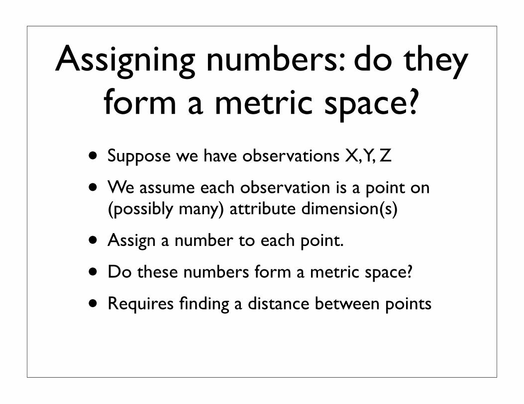
Assigning numbers: do they form a metric space?
• Suppose we have observations X, Y, Z
• We assume each observation is a point on (possibly many) attribute dimension(s)
• Assign a number to each point.
• Do these numbers form a metric space?
• Requires finding a distance between points

Metric spaces and the axioms of a distance measure
• A metric space is a set of points with a distance function, D, which meets the following properties
• Distance is symmetric, positive definite, and satisfies the triangle inequality:– D(X, Y) = D(Y, X) (symmetric)– D(X,Y) ≥ 0 (non negativity)– D(X,Y) = 0 iff X=Y (D(X,X)=0 reflexive)
– D(X,Y) + D(Y,Z) ≥ D(X,Z) (triangle inequality)

Two unidimensional metric spaces
X Y Z
X 0 1 2
Y 1 0 1
Z 2 1 0
att 1 2 3
X Y Z
X 0 3 8
Y 3 0 5
Z 8 5 0
att 1 4 9

Multidimensional spaces using alternative metrics
X Y Z WX 0 3 5 4Y 3 0 4 5Z 5 4 0 3W 4 5 3 0
Euclidian
X Y Z WX 0 3 7 4Y 3 0 4 7Z 7 4 0 3W 4 7 3 0
City block
X Y
ZW

A non metric space
X Y Z
X 0 1 2
Y 1 0 2
Z 0 0 0
att 1 1 4
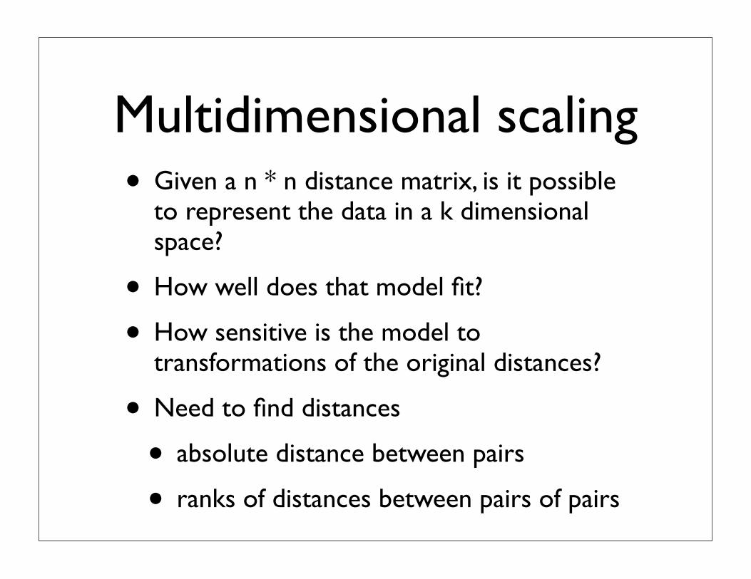
Multidimensional scaling• Given a n * n distance matrix, is it possible
to represent the data in a k dimensional space?
• How well does that model fit?
• How sensitive is the model to transformations of the original distances?
• Need to find distances
• absolute distance between pairs
• ranks of distances between pairs of pairs

Distances between US citiesBOS CHI DC DEN LA MIA NY SEA SF
BOS 0 963 429 1949 2979 1504 206 2976 3095
CHI 963 0 671 996 2054 1329 802 2013 2142
DC 429 671 0 1616 2631 1075 233 2684 2799
DEN 1949 996 1616 0 1059 2037 1771 1307 1235
LA 2979 2054 2631 1059 0 2687 2786 1131 379
MIA 1504 1329 1075 2037 2687 0 1308 3273 3053
NY 206 802 233 1771 2786 1308 0 2815 2934
SEA 2976 2013 2684 1307 1131 3273 2815 0 808
SF 3095 2142 2799 1235 379 3053 2934 808 0

Dimensional representation
Dim 1 Dim 2BOS -1349 -462CHI -428 -175DC -1077 -136
DEN 522 13LA 1464 561MIA -1227 1014NY -1199 -307SEA 1596 -639SF 1697 132

Spatial representation

A more familiar map

Compare with classic solution

Metric scaling of 28 European cities
loc <- cmdscale(eurodist)x <- loc[,1]y <- -loc[,2]plot(x, y, type="n", xlab="", ylab="", main="cmdscale(eurodist)")text(x, y, names(eurodist), cex=0.8)

Types of data collected vs. types of questions asked• Ask Si about
• O
• O x O
• infer
• O x O
• (O x O) x (O x O)
• S x O
s1 ... sn o1 ... on
s1
...sn
o1
...on

Coombs: A theory of Data
• O = {Stimulus Objects} S={Subjects}
• O = {o1, o2, …, oi, …, on}
• S = {s1, s2, …, si, …, sm}
• S x O = {(s1, o1 ) ,(si,oj), … , (sm, on)}
• O x O = {(o1, o1 ) ,(oi,oj), … , (on, on)}
• Types of Comparisons:– Order si <oj (aptitudes or amounts)
– Proximities |si -oj | < d (preferences )

Coombs typology of dataSingle Dyads Pairs of Dyads
Sing
le S
timul
iPa
irs
of S
timul
i
Measurement (S*O)si <oj
(Abilities)|si -oj | < d(attitudes)
|si -oj | < |sk -ol |
Unfolding (S*O)*(S*O)Preferential choice
oi <oj
Scaling of stimuli(O * O)
MDS(O*O)*(O*O)
|oi -oj | < |ok -ol |
Individual differences inMultidimensional Scaling
S * (O*O) * (O*O)

Coombs’ typology
• O x O (oi < oj ) Scaling
• (OxO) x (OxO) |oi - oj| < |ok - ol| MDS
• S x O (two types of comparisons)
• (si < oj) measurement of ability
• |si - oj| < d measurement of attitude
• (SxO) x (SxO) preferential choice
• |si - oj| < |sk - ol| or |si - oj| < |si - ol|

Preferential Choice and Unfolding(S * O) * (S*O)
Comparison of the distance of subject to an item versus another subject to another item:
|si -oj | < |sk -ol |
Do you like broccoli more than I like spinach?Or more typically: do you like broccoli more than you
like spinach? |si -oj | < |si -ol |
Preferential choice and Unfolding (S*O)*(S*O)

Preferential Choice: Individual (I) scales
• Question asked an individual:– Do you prefer object j to object k?
• Model of answer: – Something is preferred to something else if if it “closer” in
the attribute space or on a particular attribute dimension– Individual has an “Ideal point” on the attribute.– Objects have locations along the same attribute– |si -oj | < |si -ok |
– The I scale is the individual’s rank ordering of preferences

Preferential Choice: J scales
• Individual preferences can give information about object to object distances that are true for multiple people
• Locate people in terms of their I scales along a common J scale.

Measurement (S * O)
• Ordering of abilities: si <oj
Is a subject less than an object (i.e. does the subject miss the item).
Order the items in terms of difficulty, and subjects in terms of ability.
example: high jump or cognitive ability test
• Proximity of attitudes |si -oj | < d Subject agrees (endorses) an item if d < some threshold Subject rejects the item if d > threshold

Error free models of ability:The Guttman scale
Attribute Value ->
Res
pons
e pr
obab
ility

Errorful models of ability:Normal Ogive/Logistic of order
-3 -2 -1 0 1 2 3
0.0
0.2
0.4
0.6
0.8
1.0
Cumulative normal density for 7 items
x
pro
ba
bili
ty o
f co
rre
ct|x

Measuring Attitudes: distance from ideal point => unfolding
-3
/Users/Bill
-2 -1 0 1 2 3
0.0
0.1
0.2
0.3
0.4
Normal density for 7 items
/Users/Bill
x
pro
ba
bili
ty o
f co
rre
ct|x

Coombs typology of dataSingle Dyads Pairs of Dyads
Sing
le S
timul
iPa
irs
of S
timul
i
Measurement (S*O)si <oj
(Abilities)|si -oj | < d(attitudes)
|si -oj | < |sk -ol |
Unfolding (S*O)*(S*O)Preferential choice
oi <oj
Scaling of stimuli(O * O)
MDS(O*O)*(O*O)
|oi -oj | < |ok -ol |
Individual differences inMultidimensional Scaling
S * (O*O) * (O*O)
Scaling of people

Psychometric Theory: A conceptual SyllabusX1
X2
X3
X4
X5
X6
X7
X8
X9
Y1
Y2
Y3
Y4
Y5
Y6
Y7
Y8
L1
L2
L3
L4
L5

Measurement and scalingX1
L1
Inferring latent values from observed values

Types of Scales: Inferences from observed variables to Latent variables
• Nominal• Ordinal• Interval
• Ratio
• Categories• Ranks (x > y)• Differences– X-Y > W-V
• Equal intervals with a zero point =>– X/Y > W/V

Mappings and inferences
Observed data
Late
nt v
aria
ble
(con
stru
ct)
O1 O2 O3 O4
L1
L2
L3
L4

Ordinal Scales
• Any monotonic transformation will preserve order
• Inferences from observed to latent variable are restricted to rank orders
• Statistics: Medians, Quartiles, Percentiles

Mappings and inferences
Observed data
Late
nt v
aria
ble
(con
stru
ct)
O1 O2 O3 O4
L1
L2
L3
L4

Interval Scales
• Possible to infer the magnitude of differences between points on the latent variable given differences on the observed variableX is as much greater than Y as Z is from W
• Linear transformations preserve interval information
• Allowable statistics: Means, Variances

Mappings and inferences
Observed data
Late
nt v
aria
ble
(con
stru
ct)
O1 O2 O3 O4
L1
L2
L3
L4

Ratio Scales
• Interval scales with a zero point• Possible to compare ratios of magnitudes (X is
twice as long as Y)

The search for appropriate scale
• Is today colder than yesterday? (ranks)• Is the amount that today is colder than yesterday more than
the amount that yesterday was colder than the day before? (intervals)– 50 F - 39 F < 68 F - 50 F– 10 C - 4 C < 20 C - 10 C– 283K - 277K < 293K -283K
• How much colder is today than yesterday?– (Degree days as measure of energy use)– K as measure of molecular energy

Gas consumption by degree days (65-T)
/Users/Bill
0 10 20 30 40 50
/Users/Bill
05
10
15
Heating demands (therms) by house and Degree Days
degree days
Th
erm
s
Energy efficient with fireplace
Energy efficient no fireplace
Conventional

Latent and Observed ScoresThe problem of scale
Much of our research is concerned with making inferences about latent (unobservable) scores based upon observed measures. Typically, the relationship between observed and latent scores is monotonic, but not necessarily (and probably rarely) linear. This leads to many problems of inference. The following examples are abstracted from real studies. The names have been changed to protect the guilty.

Effect of teaching upon performance
A leading research team in motivational and educational psychology was interested in the effect that different teaching techniques at various colleges and universities have upon their students. They were particularly interested in the effect upon writing performance of attending a very selective university, a less selective university, or a two year junior college.
A writing test was given to the entering students at three institutions in the Boston area. After one year, a similar writing test was given again. Although there was some attrition from each sample, the researchers report data only for those who finished one year. The pre and post test scores as well as the change scores were as shown below:

Effect of teaching upon performance
Pretest Posttest ChangeJunior College
1 5 4Non-selectiveuniversity 5 27 22Selectiveuniversity 27 73 45
From these data, the researchers concluded that the quality ofteaching at the very selective university was much better andthat the students there learned a great deal more. Theyproposed to study the techniques used there in order to applythem to the other institutions.

Effect of Teaching upon Performance?
0
10
20
30
40
50
60
70
80
90
100
Pre PostSelective Non Selective Junior College

Another research team in motivational and educationalpsychology was interested in the effect that different teachingtechniques at various colleges and universities have upon theirstudents. They were particularly interested in the effect uponmathematics performance of attending a very selectiveuniversity, a less selective university, or a two year juniorcollege. A math test was given to the entering students atthree institutions in the Boston area. After one year, a similarmath test was given again. Although there was some attritionfrom each sample, the researchers report data only for thosewho finished one year. The pre and post test scores as well asthe change scores were:
Pretest Posttest ChangeJunior College
27 73 45Non-selectiveuniversity 73 95 22Selectiveuniversity 95 99 4

Effect of Teaching upon Performance?
0
10
20
30
40
50
60
70
80
90
100
Pre PostSelective Non Selective Junior College

A leading cognitive developmentalist believed that there is acritical stage for learning spatial representations using maps.Children younger than this stage are not helped by maps, norare children older than this stage. He randomly assigned 3rd,5th, and 7th grade students into two conditions (nested withingrade), control and map use. Performance was measured on atask of spatial recall (children were shown toys at particularlocations in a set of rooms and then asked to find them againlater. Half the children were shown a map of the rooms beforedoing the task.
No map Maps3rd grade 5 275th grade 27 737th grade 73 95

Spatial reasoning facilitated by maps at a critical age
0
10
20
30
40
50
60
70
80
90
100
3rd grade 5th grade 7th grade
No map Maps

Another cognitive developmentalist believed that there is acritical stage but that it appears earlier than previouslythought. Children younger than this stage are not helped bymaps, nor are children older than this stage. He randomlyassigned 1st, 3rd, 5th, and 7th grade students into twoconditions (nested within grade), control and map use.Performance was measured on a task of spatial recall (childrenwere shown toys at particular locations in a set of rooms andthen asked to find them again later. Half the children wereshown a map of the rooms before doing the task.
No map Maps1st grade 2 123rd grade 12 505th grade 50 887th grade 88 98

Spatial Reasoning is facilitated by map use at a critical age
0
10
20
30
40
50
60
70
80
90
100
1st grade 3rd grade 5th grade 7th grade
No map Maps

Cognitive-neuro psychologists believe that damage to thehippocampus affects long term but not immediate memory. Asa test of this hypothesis, an experiment is done in whichsubjects with and without hippocampal damage are given animmediate and a delayed memory task. The results areimpressive:
Immediate DelayedHippocampus intact 98 88Hippocampusdamaged
95 73
From these results the investigator concludes that there aremuch larger deficits for the hippocampal damaged subjects onthe delayed rather than the immediate task. The investigatorbelieves these results confirm his hypothesis. Comment on theappropriateness of this conclusion.

Memory = f(hippocampal damange * temporal delay)
0
10
20
30
40
50
60
70
80
90
100
Immediate Delayed
Hippocampus intact Hippocampus damaged

An investigator believes that caffeine facilitates attentionaltasks such that require vigilance. Subjects are randomlyassigned to conditions and receive either 0 or 4mg/kg caffeineand then do a vigilance task. Errors are recorded during thefirst 5 minutes and the last 5 minutes of the 60 minute task.The number of errors increases as the task progresses but thisdifference is not significant for the caffeine condition and is forthe placebo condition.
1st block Last blockPlacebo (0 mg/kg) 8 40Caffeine (4 mg/kg) 4 23
Errors=f(caffeine * time on task)

Errors=f(caffeine * time on task)
0
5
10
15
20
25
30
35
40
45
1st block Last block
Placebo (0 mg/kg) Caffeine (4 mg/kg)

Arousal is a fundamental concept in many psychologicaltheories. It is thought to reflect basic levels of alertness andpreparedness. Typical indices of arousal are measures of theamount of palmer sweating. This may be indexed by theamount of electricity that is conducted by the fingertips.Alternatively, it may be indexed (negatively) by the amount ofskin resistance of the finger tips. The Galvanic Skin Response(GSR) reflects moment to moment changes, SC and SR reflectlonger term, basal levels.
High skin conductance (low skin resistance) is thought toreflect high arousal.
Measuring Arousal

Anxiety is thought to be related to arousal. The following datawere collected by two different experimenters. One collectedResistance data, one conductance data.
Resistance ConductanceAnxious 2, 2 .5, .5Low anx 1, 5 1, .2
The means wereResistance Conductance
Anxious 2 .5Low anx 3 .6
Experimenter 1 concluded that the low anxious had higherresistances, and thus were less aroused. But experimenter 2noted that the low anxious had higher levels of skinconductance, and were thus more aroused.
How can this be?
Measuring Arousal

Conductance = 1/Resistance
0
0.2
0.4
0.6
0.8
1
1.2
0 1 2 3 4 5 6 7 8 9 10
Resistance
Conductance
Average Low Anxious
Average of High Anxious
Non linear response and non equal
Variances can lead to inconsistent
Inferences about group differences

420-2-40.0
0.2
0.4
0.6
0.8
1.0
Performance as a function of Ability and Test Difficulty
Ability
Performance Easy Difficult
Performance and task difficulty

Performance, ability, and task difficulty
Difficulty
Latent Ability
-4.00 0.05 0.02 0.01 0.00-2.00 0.27 0.12 0.05 0.020.00 0.73 0.50 0.27 0.122.00 0.95 0.88 0.73 0.504.00 0.99 0.98 0.95 0.88
-4 to -2 0.22 0.10 0.04 0.02-2 to -0 0.46 0.38 0.22 0.10 0 to 2 0.22 0.38 0.46 0.382 to 4 0.04 0.10 0.22 0.38
0.980.880.50
2
0.12
-2 -1 0 1
0.380.100.02
1.00Change from
0.38

Performance and Task Difficulty
Note that equal differences along the latent abilitydimension result in unequal differences along theobserved performance dimension. Compare particularlyperformance changes resulting from ability changesfrom -2 to 0 to 2 units.
This is taken from the standard logistic transformationused in Item Response Theory that maps latent abilityand latent difficulty into observed scores. IRTattempts to estimate difficulty and ability from theobserved patterns of performance.
Performance = 1/(1+exp(difficulty-abil ity) )

Decision making and the benefit of extreme selection ratios
• Typical traits are approximated by a normal distribution.• Small differences in means or variances can lead to large
differences in relative odds at the tails• Accuracy of decision/prediction is higher for extreme
values.• Do we infer trait mean differences from observing
differences of extreme values?
• (code for these graphs at • http://personality-project.org/r/extremescores.r)
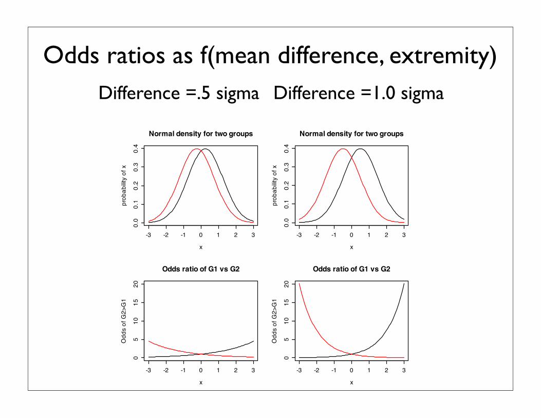
Odds ratios as f(mean difference, extremity)Difference =.5 sigma Difference =1.0 sigma
~
-3 -2 -1 0 1 2 3
0.0
0.1
0.2
0.3
0.4
Normal density for two groups
x
pro
ba
bili
ty o
f x
-3 -2 -1 0 1 2 3
05
10
15
20
Odds ratio of G1 vs G2
x
Od
ds o
f G
2>
G1
-3 -2 -1 0 1 2 3
0.0
0.1
0.2
0.3
0.4
Normal density for two groups
x
pro
ba
bili
ty o
f x
-3 -2 -1 0 1 2 3
05
10
15
20
Odds ratio of G1 vs G2
x
Od
ds o
f G
2>
G1

The effect of group differences on likelihood of extreme scoresDifference =.5 sigma Difference =1.0 sigma
-3 -2 -1 0 1 2 3
0.0
0.2
0.4
0.6
0.8
1.0
Cumulative normal density for two groups
x
pro
ba
bili
ty o
f x
-3 -2 -1 0 1 2 3
05
10
15
20
Odds ratio that person in Group exceeds x
x
Od
ds o
f G
2>
G1
-3 -2 -1 0 1 2 3
0.0
0.2
0.4
0.6
0.8
1.0
Cumulative normal density for two groups
x
pro
ba
bili
ty o
f x
-3 -2 -1 0 1 2 3
05
10
15
20
Odds ratio that person in Group exceeds x
x
Od
ds o
f G
2>
G1

The effect of differences of variance on odds ratios at the tails
-3 -2 -1 0 1 2 3
0.0
0.1
0.2
0.3
0.4
variance of two groups differ by 10%
x
pro
ba
bili
ty o
f x
-3 -2 -1 0 1 2 3
0.0
1.0
2.0
3.0
Odds ratio of G1 vs G2
x
Od
ds o
f G
2>
G1
-3 -2 -1 0 1 2 3
0.0
0.1
0.2
0.3
0.4
Variance of two groups differs by 20%
x
pro
ba
bili
ty o
f x
-3 -2 -1 0 1 2 3
0.0
1.0
2.0
3.0
Odds ratio of G1 vs G2
x
Od
ds o
f G
2>
G1

Percentiles are not a linear metricand percentile odds are even worse!
• When comparing changes due to interventions or environmental trends, it is tempting to see how many people achieve a certain level (eg., of educational accomplishment, or of obesity), but the magnitude of such changes are sensitive to starting points, particularly when using percentiles or even worse, odds of percentiles.
• Consider the case of obesity:
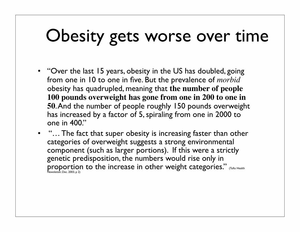
Obesity gets worse over time
• “Over the last 15 years, obesity in the US has doubled, going from one in 10 to one in five. But the prevalence of morbid obesity has quadrupled, meaning that the number of people 100 pounds overweight has gone from one in 200 to one in 50. And the number of people roughly 150 pounds overweight has increased by a factor of 5, spiraling from one in 2000 to one in 400.”
• “… The fact that super obesity is increasing faster than other categories of overweight suggests a strong environmental component (such as larger portions). If this were a strictly genetic predisposition, the numbers would rise only in proportion to the increase in other weight categories.” (Tufts Health Newsletter, Dec. 2003, p 2)

Is obesity getter worse for the super obese? - Seemingly
Label Definition Odds Change in Odds
Obese BMI = 3040 lb for 5’5”
1/10 to 1/5
2
Morbid Obese
BMI = 40100 lb
1/200 to1/50
4
Super Obese
BMI = 50150 lb
1/2000 to1/400
5

Is obesity getter worse for the super obese? -- No
Label Definition Odds Change in Odds
z score Change in z
Obese BMI = 30 1/10 to 1/5
2 -1.28 -.84
.44
Morbid Obese
BMI = 40 1/200 to1/50
4 -2.58-2.05
.53
Super Obese
BMI = 50 1/2000 to1/400
5 -3.29-2.81
.48

Psychometric Theory: A conceptual SyllabusX1
X2
X3
X4
X5
X6
X7
X8
X9
Y1
Y2
Y3
Y4
Y5
Y6
Y7
Y8
L1
L2
L3
L4
L5