psychological test and assessment modeling, volume 60, … test and assessment modeling, volume 60,...
TRANSCRIPT

Psychological Test and Assessment Modeling, Volume 60, 2018 (1), 29-32
Guest Editorial Rater effects: Advances in item response modeling of human ratings – Part II Thomas Eckes1
The papers in Part I of this special issue dealt with rater effects from the perspective of two-facet IRT modeling (Wu, 2017), multilevel, hierarchical rater models (Casabianca & Wolfe, 2017), and nonparametric Mokken analysis (Wind & Engelhard, 2017). Part II includes papers that probe further into the complex nature of human ratings within the context of performance assessment, highlighting the benefits and challenges of examin-ing rater effects from different angles and with different levels of detail. In the first paper, entitled “A tale of two models: Psychometric and cognitive perspec-tives on rater-mediated assessments using accuracy ratings”, George Engelhard, Jue Wang, and Stefanie A. Wind elaborate on the need to bring together psychometric and cognitive perspectives in order to gain a deeper understanding of rater-mediated as-sessments (Engelhard, Wang, & Wind, 2018). Whereas psychometric perspectives have long dominated the field, cognitive perspectives with their specific focus on the study of human categorization, judgment, and decision making in assessment contexts have only recently attracted more attention (Bejar, 2012). In the paper, Engelhard et al. build on Brunswik’s (1952) lens model as a cognitive approach and conceptually link this model to many-facet Rasch measurement (MFRM; Linacre, 1989). Their study is situated within an external frame of reference, that is, a group of experts provided criterion rat-ings that were compared to operational ratings to obtain rating accuracy data. Using the Rater Accuracy Model (RAM; Engelhard, 1996), the authors construct measures for the accuracy of individual raters in a writing assessment and analyze which examinee per-formances and writing domains, respectively, were difficult to rate accurately. In the second paper, entitled “Modeling rater effects using a combination of generaliza-bility theory and IRT”, Jinnie Choi and Mark R. Wilson adopt a generalized linear latent and mixed model (GLLAMM) approach to combine what many researchers and assessment specialists have considered fundamentally different methods to study rating quality (Choi & Wilson, 2018). As discussed in the Editorial to Part I (Eckes, 2017),
1Correspondence concerning this article should be addressed to: Thomas Eckes, PhD, TestDaF Institute,
University of Bochum, Universitätsstr. 134, 44799 Bochum, Germany; email: [email protected]

T. Eckes
30
generalizability theory (GT; e.g., Brennan, 2001) and IRT are commonly thought to represent diverging research traditions. Simply put, GT, being rooted in classical test theory and analysis of variance, focuses on observed test scores, whereas IRT focuses on item responses and how they relate to the ability being measured (Brennan, 2011; Linacre, 2001). Against this background, Choi and Wilson demonstrate that much is to be gained from integrating both approaches into a logistic mixed model that allows not only to estimate random variance components and generalizability coefficients for ex-aminees, items, and raters, but also to construct individual examinee, item, and rater measures as known from IRT applications (see also Robitzsch & Steinfeld, 2018a). Further advantages of the combined approach refer to its flexibility regarding the analy-sis of multidimensional and/or polytomous item response data and the graphical presen-tation of predicted individual random effects in modified Wright maps. In the third paper, entitled “Comparison of human rater and automated scoring of test takers’ speaking ability and classification using item response theory”, Zhen Wang and Yu Sun provide a detailed look at the performance of an automated scoring system for spoken responses (Wang & Sun, 2018). Specifically, the authors use the automated scoring engine SpeechRater, developed at Educational Testing Service (ETS), to score examinee performances on the speaking section of an English language assessment, and compare the scores from SpeechRater to scores assigned by human raters. Wang and Sun consider a range of scoring scenarios representing various combinations of SpeechRater and human ratings, such as human rater only, SpeechRater only, and dif-ferential weighting of SpeechRater and human rater contributions to the final scores. Building on structural equation modeling and IRT scaling (GPCM; Muraki, 1992), the authors find pronounced differences between the results obtained for each of these scenarios, indicating that automated scores and human rater scores of spoken responses do not reflect the same underlying construct. The final paper, entitled "Item response models for human ratings: Overview, estima-tion methods, and implementation in R" by Alexander Robitzsch and Jan Steinfeld, first provides a brief introduction to IRT models for human ratings, including many-facet rater models based on partial credit, generalized partial credit, and graded response modeling approaches, as well as generalized many-facet rater models, covariance struc-ture models, and hierarchical rater models (Robitzsch & Steinfeld, 2018a). The authors go on to present various maximum likelihood and Bayesian methods of estimating parameters for each of these models. Following a thoughtful discussion of how to choose between the different models, Robitzsch and Steinfeld illustrate the practical model use with a real data set. For this purpose, they draw on three different, highly versatile R packages for estimating IRT models for multiple raters: "immer" (Item Re-sponse Models for Multiple Ratings; Robitzsch & Steinfeld, 2018b), "sirt" (Supplemen-tary Item Response Theory Models; Robitzsch, 2018), and "TAM" (Test Analysis Modules; Robitzsch, Kiefer, & Wu, 2018). The findings from these analyses are com-pared with linear mixed effects models implemented in the “lme4” package (Bates, Mächler, Bolker, & Walker, 2015). For each data analysis, the authors provide excerpts from the R syntax along with detailed explanations in order to guide readers in how to best use the R packages with their own research.

Rater effects – Guest Editorial (Part II)
31
Taken together, the psychometric approaches, models, and analyses documented in Parts I and II provide new insights into rater effects across a wide range of assessment contexts. It seems evident that item response modeling has made much progress both in terms of detecting rater effects and mitigating or even correcting at least part of the negative impact these effects have on the validity and fairness of human ratings. May these advances stimulate not only future research in the field, but also inform practical decisions regarding the design, implementation, and evaluation of rater-mediated as-sessments.
References
Bates, D., Mächler, M., Bolker, B., & Walker, S. (2015). Fitting linear mixed-effects mod-els using lme4. Journal of Statistical Software, 67(1).
Bejar, I. I. (2012). Rater cognition: Implications for validity. Educational Measurement: Issues and Practice, 31(3), 2–9.
Brennan, R. L. (2001). Generalizability theory. New York, NY: Springer.
Brennan, R. L. (2011). Generalizability theory and classical test theory. Applied Measure-ment in Education, 24, 1–21.
Brunswik, E. (1952). The conceptual framework of psychology. Chicago, IL: University of Chicago Press.
Casabianca, J. M., & Wolfe, E. W. (2017). The impact of design decisions on measurement accuracy demonstrated using the hierarchical rater model. Psychological Test and As-sessment Modeling, 59(4), 471–492.
Choi, J., & Wilson, M. R. (2018). Modeling rater effects using a combination of generali-zability theory and IRT. Psychological Test and Assessment Modeling, 60(1), 53–80.
Eckes, T. (2017). Rater effects: Advances in item response modeling of human ratings – Part I (Guest Editorial). Psychological Test and Assessment Modeling, 59(4), 443–452.
Engelhard, G. (1996). Evaluating rater accuracy in performance assessments. Journal of Educational Measurement, 33, 56–70.
Engelhard, G., Wang, J., & Wind, S. A. (2018). A tale of two models: Psychometric and cognitive perspectives on rater-mediated assessments using accuracy ratings. Psycho-logical Test and Assessment Modeling, 60(1) 33–52.
Linacre, J. M. (1989). Many-facet Rasch measurement. Chicago, IL: MESA Press.
Linacre, J. M. (2001). Generalizability theory and Rasch measurement. Rasch Measurement Transactions, 15, 806–807.
Muraki, E. (1992). A generalized partial credit model: Application of an EM algorithm. Applied Psychological Measurement, 16, 159–176.
Robitzsch, A. (2018). Package ‘sirt’: Supplementary item response theory models (Version 2.5) [Computer software and manual]. Retrieved from https://cran.r-project.org/web/packages/sirt/index.html

T. Eckes
32
Robitzsch, A., Kiefer, T., & Wu, M. (2018). Package ‘TAM’: Test analysis modules (Ver-sion 2.9) [Computer software and manual]. Retrieved from https://cran.r-project.org/web/packages/TAM/index.html
Robitzsch, A., & Steinfeld, J. (2018a). Item response models for human ratings: Overview, estimation methods and implementation in R. Psychological Test and Assessment Mod-eling, 60(1), 101–138.
Robitzsch, A., & Steinfeld, J. (2018b). Package ‘immer’: Item response models for multiple ratings (Version 1.0) [Computer software and manual]. Retrieved from https://cran.r-project.org/web/packages/immer/index.html
Wang, Z., & Sun, Y. (2018). Comparison of human rater and automated scoring of test takers’ speaking ability and classification using item response theory. Psychological Test and Assessment Modeling, 60(1), 81–100.
Wind, S. A., & Engelhard, G. (2017). Exploring rater errors and systematic biases using adjacent-categories Mokken models. Psychological Test and Assessment Modeling, 59(4), 493–515.
Wu, M. (2017). Some IRT-based analyses for interpreting rater effects. Psychological Test and Assessment Modeling, 59(4), 453–470.

Psychological Test and Assessment Modeling, Volume 60, 2018 (1), 33-52
A tale of two models: Psychometric and cognitive perspectives on rater-mediated assessments using accuracy ratings George Engelhard, Jr1, Jue Wang2, & Stefanie A. Wind3
Abstract The purpose of this study is to discuss two perspectives on rater-mediated assessments: psychometric and cognitive perspectives. In order to obtain high quality ratings in rater-mediated assessments, it is essential to be guided by both perspectives. It is also important that the specific models selected are congruent and complementary across perspectives. We discuss two measurement models based on Rasch measurement theory (Rasch, 1960, 1980) to represent the psychometric perspective, and we emphasize the Rater Accuracy Model (Engelhard, 1996, 2013). We build specific judgment models to reflect the cognitive perspective of rater scoring processes based on Brunswik's Lens model frame-work. We focus on differential rater functioning in our illustrative analyses. Raters who possess in-consistent perceptions may provide different ratings, and this may cause various types of inaccuracy. We use a data set that consists of the ratings of 20 operational raters and three experts of 100 essays written by Grade 7 students. Student essays were scored using an analytic rating rubric for two do-mains: (1) idea, development, organization, and cohesion; as well as (2) language usage and conven-tion. Explicit consideration of both psychometric and cognitive perspectives has important implica-tions for rater training and maintaining the quality of ratings obtained from human raters.
Keywords: Rater-mediated assessments, Rasch measurement theory, Lens model, Rater judgment, Rater accuracy
1Correspondence concerning this article should be addressed to: George Engelhard, Jr., Ph.D., Professor
of Educational Measurement and Policy, Quantitative Methodology Program, Department of Educa-tional Psychology, 325W Aderhold Hall, The University of Georgia, Athens, Georgia 30602, U.S.A. email: [email protected]
2The University of Georgia 3The University of Alabama
G. Engelhard, Jr., J. Wang , & S. A. Wind 34
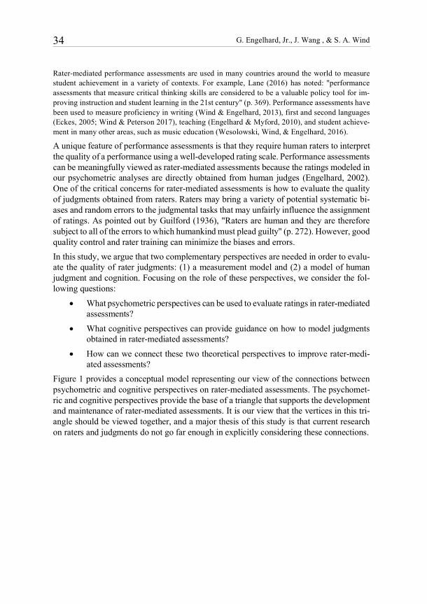
Rater-mediated performance assessments are used in many countries around the world to measure student achievement in a variety of contexts. For example, Lane (2016) has noted: "performance assessments that measure critical thinking skills are considered to be a valuable policy tool for im-proving instruction and student learning in the 21st century" (p. 369). Performance assessments have been used to measure proficiency in writing (Wind & Engelhard, 2013), first and second languages (Eckes, 2005; Wind & Peterson 2017), teaching (Engelhard & Myford, 2010), and student achieve-ment in many other areas, such as music education (Wesolowski, Wind, & Engelhard, 2016).
A unique feature of performance assessments is that they require human raters to interpret the quality of a performance using a well-developed rating scale. Performance assessments can be meaningfully viewed as rater-mediated assessments because the ratings modeled in our psychometric analyses are directly obtained from human judges (Engelhard, 2002). One of the critical concerns for rater-mediated assessments is how to evaluate the quality of judgments obtained from raters. Raters may bring a variety of potential systematic bi-ases and random errors to the judgmental tasks that may unfairly influence the assignment of ratings. As pointed out by Guilford (1936), "Raters are human and they are therefore subject to all of the errors to which humankind must plead guilty" (p. 272). However, good quality control and rater training can minimize the biases and errors. In this study, we argue that two complementary perspectives are needed in order to evalu-ate the quality of rater judgments: (1) a measurement model and (2) a model of human judgment and cognition. Focusing on the role of these perspectives, we consider the fol-lowing questions:
• What psychometric perspectives can be used to evaluate ratings in rater-mediated assessments?
• What cognitive perspectives can provide guidance on how to model judgments obtained in rater-mediated assessments?
• How can we connect these two theoretical perspectives to improve rater-medi-ated assessments?
Figure 1 provides a conceptual model representing our view of the connections between psychometric and cognitive perspectives on rater-mediated assessments. The psychomet-ric and cognitive perspectives provide the base of a triangle that supports the development and maintenance of rater-mediated assessments. It is our view that the vertices in this tri-angle should be viewed together, and a major thesis of this study is that current research on raters and judgments do not go far enough in explicitly considering these connections.

A tale of two models 35
Figure 1:
Conceptual model for rater-mediated assessments
What psychometric perspectives can be used to evaluate ratings in rater-mediated assessments?
In evaluating the quality of ratings, there have been several general perspectives. These psychometric perspectives can be broadly classified into test score and scaling traditions (Engelhard, 2013). Many of the current indices used in operational testing to evaluate rat-ings are based on the test score tradition; for example, rater agreement indices, intraclass correlations, kappa coefficients, and generalizability coefficients (Cronbach, Gleser, Nanda, & Rajaratnam, 1972; Johnson, Penny & Gordon, 2009; von Eye, & Mun, 2005). It is safe to say that most operational performance assessment systems report the percentage of exact and adjacent category usage for operational raters. All of these models within the test score tradition treat the observed ratings as having categories with equal width. In other words, the ratings are modeled as equal intervals by using sum scores. Ratings can also be evaluated using measurement models based on the scaling tradition (Engelhard, 2013). In the scaling tradition, the structure of rating categories is parameter-ized with category coefficients (i.e., thresholds). Thresholds that define rating categories are not necessarily of equal width (Engelhard & Wind, 2013). The most common IRT models for rating scale analysis include the Partial Credit Model (Masters, 1982), the Rat-ing Scale Model (Andrich, 1978), the Generalized Partial Credit Model (Muraki, 1992), and the Graded Response Model (Samejima, 1969). The Many-Facet Rasch model (Lina-cre, 1989) specifically adds a rater parameter, and this model is widely used in the detec-tion of rater effects. The Many-Facet Rasch model is a generalized form of the Rasch model that was specifically designed for rater-mediated assessments (Eckes, 2015). There are also several other rater models, such as the hierarchical rater model (Casabiaca, Junker, & Patz, 2016), that have been proposed. It is beyond the scope of this study to describe in detail other models for ratings, and we recommend Nering and Ostini (2010) for interested readers.

G. Engelhard, Jr., J. Wang , & S. A. Wind 36
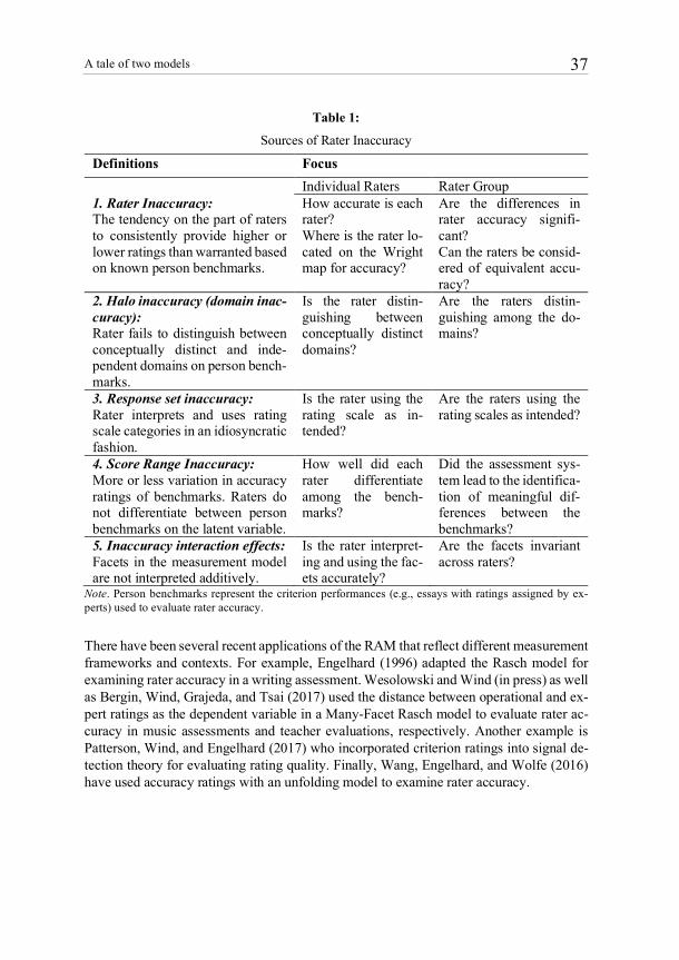
All of the psychometric perspectives described up to this point model the observed ratings assigned by raters. Engelhard (1996) proposed another approach based on accuracy ratings (Wolfe, Jiao, & Song, 2014). Accuracy ratings represent the distances between criterion ratings and operational ratings. For instance, criterion ratings are assigned by an expert rater or a group of expert raters. The observed ratings assigned by well-trained operational raters are referred to as operational ratings. The differences between these operational rat-ings and criterion ratings reflect the accuracy of operational rater judgments on each per-formance. Engelhard (1996) put forward an equation for calculating accuracy ratings. Since accuracy ratings reflect the distance between operational ratings and criterion rat-ings, we call them direct measures of rater accuracy. On the other hand, observed opera-tional ratings are viewed as indirect measures for rater accuracy. Due to this difference, we use the term Rater Accuracy Models (RAM) to label the Rasch models that examine accuracy ratings as the dependent variable on which individual raters, performances, and other facets can be measured. We present two lens models for observed operational ratings and accuracy ratings correspondingly. Scholars have used the term rater accuracy in numerous ways to describe a variety of rating characteristics, including agreement, reliability, and model-data fit (Wolfe & McVay, 2012). In these applications, rater accuracy is used as a synonym for ratings with desirable psychometric properties. RAM provides a criterion-referenced perspective on rating quality that can be used to directly describe and compare individual raters, perfor-mances, and other facets in the assessment system with a focus on rater accuracy. From criterion-referenced perspective, the RAM provides a more specific definition and clear interpretation of rater accuracy. Furthermore, the criterion-referenced approach empha-sizes the evaluation of rater accuracy using accuracy ratings as direct measures. These accuracy ratings can be coupled with a lens model to guide rater training and diagnostic activities during scoring. We summarize five sources of inaccuracy due to differences among rater judgments in Table 1. First, we view rater inaccuracy as a tendency to consistently provide biased rat-ings. Second, halo inaccuracy or domain inaccuracy refers to the situations that raters fail to distinguish among different domains on an analytic scoring rubric when evaluating stu-dent performances. Wang, Engelhard, Raczynski, Song, and Wolfe (2017) observed this phenomenon that some raters tended to provide adjacent scores for two distinct domains of writing. Third, when raters use the rating scale in an idiosyncratic fashion, it leads to response set inaccuracy such that ratings are not consistent toward the benchmarks used as the basis for criterion ratings. Specifically, person benchmarks refer to the pre-calibrated performances (e.g., students’ essays) that are used to evaluate raters’ scoring proficiency. Fourth, score range inaccuracy occurs when ratings have less or more variation than ex-pected based on the measurement model. Lastly, if raters interpret other facets differen-tially, interaction effects may appear in rater inaccuracy. It should also be noted that the focus (i.e., individual raters versus rater groups) yields different questions and conclusions related to rater inaccuracy. These sources of rater inaccuracy can guide researchers in iden-tifying possible sources of rater inaccuracy with the use of RAM or other psychometric models.
A tale of two models 37
Table 1:
Sources of Rater Inaccuracy
Definitions Focus Individual Raters Rater Group 1. Rater Inaccuracy: The tendency on the part of raters to consistently provide higher or lower ratings than warranted based on known person benchmarks.
How accurate is each rater? Where is the rater lo-cated on the Wright map for accuracy?
Are the differences in rater accuracy signifi-cant? Can the raters be consid-ered of equivalent accu-racy?
2. Halo inaccuracy (domain inac-curacy): Rater fails to distinguish between conceptually distinct and inde-pendent domains on person bench-marks.
Is the rater distin-guishing between conceptually distinct domains?
Are the raters distin-guishing among the do-mains?
3. Response set inaccuracy: Rater interprets and uses rating scale categories in an idiosyncratic fashion.
Is the rater using the rating scale as in-tended?
Are the raters using the rating scales as intended?
4. Score Range Inaccuracy: More or less variation in accuracy ratings of benchmarks. Raters do not differentiate between person benchmarks on the latent variable.
How well did each rater differentiate among the bench-marks?
Did the assessment sys-tem lead to the identifica-tion of meaningful dif-ferences between the benchmarks?
5. Inaccuracy interaction effects: Facets in the measurement model are not interpreted additively.
Is the rater interpret-ing and using the fac-ets accurately?
Are the facets invariant across raters?
Note. Person benchmarks represent the criterion performances (e.g., essays with ratings assigned by ex-perts) used to evaluate rater accuracy.
There have been several recent applications of the RAM that reflect different measurement frameworks and contexts. For example, Engelhard (1996) adapted the Rasch model for examining rater accuracy in a writing assessment. Wesolowski and Wind (in press) as well as Bergin, Wind, Grajeda, and Tsai (2017) used the distance between operational and ex-pert ratings as the dependent variable in a Many-Facet Rasch model to evaluate rater ac-curacy in music assessments and teacher evaluations, respectively. Another example is Patterson, Wind, and Engelhard (2017) who incorporated criterion ratings into signal de-tection theory for evaluating rating quality. Finally, Wang, Engelhard, and Wolfe (2016) have used accuracy ratings with an unfolding model to examine rater accuracy.

G. Engelhard, Jr., J. Wang , & S. A. Wind 38
What cognitive perspectives can provide guidance on how to model judgments obtained in rater-mediated assessments?
The simple beauty of Brunswik's lens model lies in recognizing that the per-son's judgment and the criterion being predicted can be thought of as two
separate functions of cues available in the environment of the decision. (Karelaia and Hogarth, 2008, p. 404)
Cognitive psychology (Barsalou, 1992) offers a variety of options for considering judg-ment and decision-making tasks related to rater-mediated assessments. Cooksey (1996) describes 14 theoretical perspectives on judgment and decision making that can be poten-tial models for examining the quality of judgments in rater-mediated assessments. Within educational settings, there was a special issue of Educational Measurement: Issues and Practice devoted to rater cognition (Leighton, 2012). There are many promising areas for future research on rater cognition and rater judgments (Lane, 2016; Myford, 2012; Wolfe, 2014). Although there are numerous potential models of human judgment that may be useful guides for monitoring rating quality, the underlying model of judgmental processes used here is based on Brunswik's (1952) lens model. Lens models have been used extensively used across social science research contexts to examine human judgments. For example, there are two important meta-analyses of research organized around lens models. First, Karelaia and Hogarth (2008) conducted a meta-analysis of five decades of lens model studies (N=249) that included a variety of task environments. More recently, Kaufmann, Reips, and Wittmann (2013) conducted a meta-analysis based on 31 lens model studies including applications from medicine, business, education, and psychology. An important resource for recent work on lens models is the website of the Brunswik Society (http://www.brunswik.org/), which provides yearly abstracts of current research utilizing a lens model framework. Brunswik (1952, 1955a, 1955b, 1956) proposed a new perspective in psychology called probabilistic functionalism (Athanasou & Kaufmann, 2015; Postman & Tolman, 1959). An important aspect of Brunswik's research was the concept of a lens model (Hammond, 1955; Postman & Tolman, 1959). The structure of Brunswik’s lens models varied over time and application areas. Figure 2 presents a lens model for perception proposed by Brunswik (1955a). In this case, a person utilizes a set of cues (i.e., proximal-peripheral cues) to generate a response (i.e., central response). The accuracy of a person's response can be evaluated by its relationship to the distal variable, which is called functional valid-ity. Ecological validities represent the relationships between the distal variable and the cues, while utilization validities reflect the relationship between the cues and the central response. In both cases, higher values of correspondence are viewed as evidence of valid-ity. It is labeled a lens model because it resembles the way light passes through a lens defined by cues.

A tale of two models 39
Figure 2:
Lens model for perception constancy (Adopted from Brunswik (1955a, p. 206)
In rater-mediated assessments, the accuracy of a rater’s response (i.e., observed rating) is evaluated by its correspondence to or relationship with the latent variable (i.e., distal var-iable). Engelhard (1992, 1994, 2013) adapted the lens model as a conceptual framework for rater judgments in writing assessment. Figure 3 provides a bifocal perspective on rater accuracy in measuring writing competence. We refer to Figure 3 as Lens Model I, where the basic idea is that the latent variable — writing competence — is made visible through a set of cues or intervening variables (e.g., essay features, domains, and rating scale us-ages) that are interpreted separately by experts and operational raters. Our goal in this case is to have a close correspondence between the measurement of the latent variable (i.e., writing competence) between expert and operational raters. Judgmental accuracy in Lens Model I refers to the closeness between rater’s operational ratings and experts’ criterion ratings of student performances including their interpretations of the cues. Wang and Engelhard (2017) applied Lens model I to evaluate rating quality in writing assessments.
Figure 3:
Lens model I (bifocal model) for measuring writing competence
In contrast to Lens Model I, the current study focuses on a slightly different definition of a lens model. Specifically, we focus on Lens Model II (see Figure 4). In Lens Model II, the latent variable is rater accuracy instead of writing competence in the assessment

G. Engelhard, Jr., J. Wang , & S. A. Wind 40
system. The goal is to evaluate accuracy ratings (i.e., differences between observed and criterion ratings) as responses of raters in the judgmental system. These accuracy ratings can be distinguished from the ratings modeled separately for expert and operational raters in Lens Model I.
Figure 4:
Lens model II for measuring rater accuracy
As pointed out in the opening quote for this section, a defining feature of lens models is that they include two separate functions reflecting judgment and criterion systems. Brunswik (1952) primarily used correlational analyses to examine judgmental data. Mul-tiple regression analyses are currently the most widely used method for examining data from lens-model studies of judgments (Cooksey, 1996). It is interesting to note that Ham-mond (1996) suggested that lens-model research may have overemphasized the role of multiple regression techniques, and that the "lens model is indifferent — a priori — to which organizing principle is employed in which task under which circumstances; it con-siders that to be an empirical matter" (p. 245). In our study, we suggest using psychometric models based on Rasch measurement theory and invariant measurement as an organizing principle (Engelhard, 2013). As pointed out earlier, the majority of analyses conducted with lens models are regression-based analyses. Lens Model I reflects this perspective very closely with the Rasch model substituted for multiple regression analyses.
How can we connect these two perspectives to improve rater-mediated assessments?
Accuracy …refers to closeness of an observation to the quality intended to be observed
(Kendall & Buckland, 1957, p. 224) Researchers have adopted several different statistical approaches for analyzing data for lens-model studies. First, the ratings have been modeled directly using correlational and multiple regression analyses (Brunswik 1952; Cooksey, 1996; Hammond, Hursch, and Todd, 1964; Hursch, Hammond, & Hursch, 1964; Tucker, 1964). Cooksey (1986) pro-vided an informative example of using a lens model approach to examine teacher judg-ments of student reading achievement. In this study, student scores on standardized read-ing achievement tests define the ecological or criterion system with three cues (i.e., social economic status, reading ability, and oral language ability). In a similar fashion, the

A tale of two models 41
judgmental system was defined based on the relationship between teacher judgments and the same set of cues. Regression-based indices were used to compare the ecological and judgmental systems. Cooksey, Freebody, and Wyatt-Smith (2007) also applied a lens model to study teacher’s judgments of writing achievement. The drawback of this meth-odology is that each person’s judgment is compared against the criterion individually; that said, separate regression analyses are required for each judge. A second approach is to use IRT models that are developed within the scaling tradition. Researchers can obtain individual-level estimates using various IRT models in one analy-sis instead of separate multiple-regression analyses. For example, Engelhard (2013) pro-posed the use of a Many-Facet Rasch Model to examine the lens model I for measuring writing proficiency. Finally, it is possible to model the criterion and judgmental systems as the distances be-tween the ratings from each system. The lens model for measuring rater accuracy based on this approach can be best represented by the RAM. RAM has been proposed and applied to evaluate rater accuracy in writing assessments (Engelhard, 1996, 2013; Wolfe, Jiao, & Song, 2014). We illustrate the correspondence between the Lens Model II and the RAM. Specifically, we use the distances between the ratings of expert raters and the operational raters to define accuracy ratings which are analyzed in the judgment system of Lens Model II. RAM analyzes the accuracy ratings that are direct measures of rater accuracy. In addition, there are several advantages of using Rasch measurement theory over regres-sion-based approaches for judgment studies. First of all, multiple regression analyses may lead to a piecemeal approach with an array of separate analyses. Cooksey (1996) provides ample illustrations of these types of analyses within the context of judgment studies. Our approach based on Rasch measurement theory provides a coherent view for analyzing rater-mediated assessments. Second, it is hard to substantively conceptualize the focal point (i.e., object of measurement) when a regression-based approach is used. In this study, we describe two Rasch-based approaches that focus on either students or raters as the ob-ject of measurement. Our approach offers the advantages of obtaining invariant indicators of rating quality under appropriate conditions. Lastly, we would like to stress the value of Wright Maps that define an underlying continuum, and provide the opportunity to visual-ize and understand rater-mediated measurement as a line representing the construct or la-tent variable of interest.
Illustrative data analyses
In this study, we use illustrative data analyses to highlight the use of the RAM and Brunswikian lens model as a promising way to bring together psychometric and cognitive perspectives related to evaluating rater judgments. Specifically, we conducted a secondary data analysis with the use of RAM to examine differential rater functioning as one of the sources causing inaccurate ratings through the lens. The data, which were originally col-lected and analyzed by Wang, Engelhard, Raczynski, Song, and Wolfe (2017), were part of a statewide writing assessment program for Grade 7 students in a southeastern state of the United States.

G. Engelhard, Jr., J. Wang , & S. A. Wind 42
Participants
According to Wang et al. (2017)’s data collection procedure, twenty well-trained opera-tional raters were randomly chosen from a larger rater pool. The group of raters scored a random sample of 100 essays. This set of essays was used as training essays to evaluate rater performance prior to the actual operational scoring. The design was fully crossed with all of the raters rating all of the essays. A panel of three experts who provided the training and picked the training essays assigned the criterion ratings for these 100 essays.
Instrument
The writing assessment was document based, that is students were asked to write an essay based on a prompt. The essays were scored analytically in two domains: (a) idea develop-ment, organization, and coherence (IDOC Domain), and (b) language usage and conven-tions (LUC Domain). IDOC Domain was scored using a category of 0-4, and LUC domain was rated from 0-3. A higher score indicates better proficiency in a specific writing do-main.
Procedures
In our study, exact matches between operational and criterion ratings from the panel of expert raters are assigned an accuracy rating of 1, while other discrepancies are assigned a 0. Higher scores reflect higher levels scoring accuracy for raters. In other words, accu-racy ratings are dichotomized (0=inaccurate rating, 1=accurate ratings). The RAM includes three facets: Raters, essays and domains. We used the Facets computer program (Linacre, 2015) to analyze the dichotomous accuracy ratings. The general RAM model can be expressed as follows:
Ln[Pnmik / Pnmik-1] = bn – dm – li – tk (1)
where Pnmik = probability of rater n assigning an accurate rating to benchmark essay m for
domain i, Pnmik-1 = probability of rater n assigning an inaccurate rating to benchmark essay m for
domain i, bn = accuracy of rater n, dm = difficulty of assigning an accurate rating to benchmark essay m, li = difficulty of assigning an accurate rating for domain i, and tk = difficulty of accuracy-rating category k relative to category k-1.
A tale of two models 43
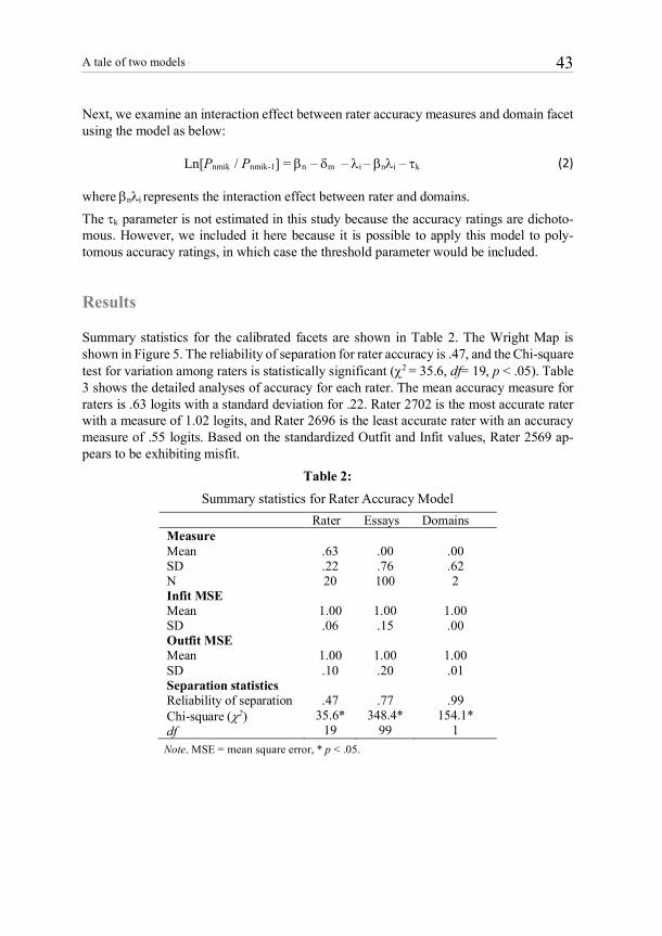
Next, we examine an interaction effect between rater accuracy measures and domain facet using the model as below:
Ln[Pnmik / Pnmik-1] = bn – dm – li – bnli – tk (2)
where bnli represents the interaction effect between rater and domains. The tk parameter is not estimated in this study because the accuracy ratings are dichoto-mous. However, we included it here because it is possible to apply this model to poly-tomous accuracy ratings, in which case the threshold parameter would be included.
Results
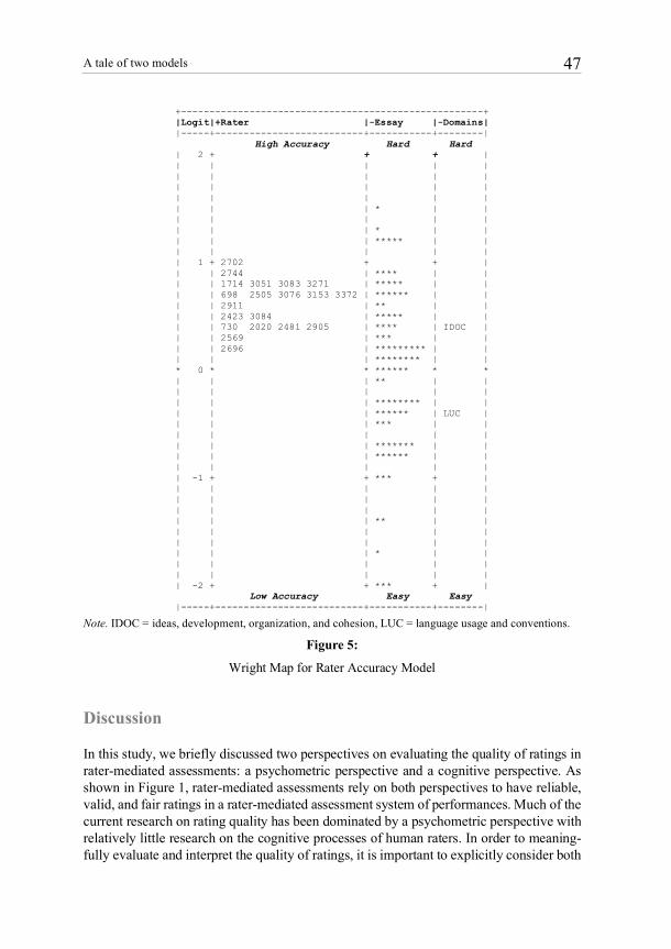
Summary statistics for the calibrated facets are shown in Table 2. The Wright Map is shown in Figure 5. The reliability of separation for rater accuracy is .47, and the Chi-square test for variation among raters is statistically significant (c2 = 35.6, df= 19, p < .05). Table 3 shows the detailed analyses of accuracy for each rater. The mean accuracy measure for raters is .63 logits with a standard deviation for .22. Rater 2702 is the most accurate rater with a measure of 1.02 logits, and Rater 2696 is the least accurate rater with an accuracy measure of .55 logits. Based on the standardized Outfit and Infit values, Rater 2569 ap-pears to be exhibiting misfit.
Table 2: Summary statistics for Rater Accuracy Model
Rater Essays Domains Measure Mean SD N
.63 .22 20
.00 .76 100
.00 .62 2
Infit MSE Mean SD
1.00 .06
1.00 .15
1.00 .00
Outfit MSE Mean SD
1.00 .10
1.00 .20
1.00 .01
Separation statistics Reliability of separation Chi-square (c2) df
.47
35.6* 19
.77
348.4* 99
.99
154.1* 1
Note. MSE = mean square error, * p < .05.

G. Engelhard, Jr., J. Wang , & S. A. Wind 44
Table 3:
Accuracy measures and fit statistics for raters
Rater ID Accuracy (Prop.)
Measure (Logits)
S.E. Infit MSE
Infit Z
Outfit MSE
Outfit Z
Slope
2702 0.70 1.02 0.17 1.07 1.01 1.10 0.86 0.84 2744 0.69 0.91 0.16 0.98 -0.21 0.92 -0.76 1.07
3051 0.67 0.83 0.16 1.05 0.78 1.16 1.53 0.84
3271 0.67 0.83 0.16 1.07 1.10 1.08 0.76 0.82
1714 0.66 0.81 0.16 0.95 -0.82 0.92 -0.79 1.14 2505 0.65 0.73 0.16 0.99 -0.19 0.97 -0.26 1.04
3076 0.65 0.73 0.16 0.99 -0.13 0.98 -0.16 1.03
3083 0.65 0.76 0.16 1.03 0.42 1.06 0.66 0.91
3372 0.65 0.73 0.16 1.04 0.59 1.00 -0.01 0.93
698 0.64 0.70 0.16 0.90 -1.76 0.84 -1.79 1.31
3153 0.64 0.70 0.16 0.91 -1.49 0.86 -1.52 1.26
2911 0.63 0.63 0.16 0.93 -1.26 0.89 -1.20 1.23
2423 0.61 0.53 0.16 0.99 -0.15 1.04 0.54 1.00
3084 0.60 0.48 0.16 0.97 -0.57 0.93 -0.87 1.13
2020 0.59 0.44 0.15 0.96 -0.81 0.93 -0.82 1.16
2905 0.58 0.41 0.15 0.98 -0.39 0.95 -0.59 1.09
730 0.57 0.36 0.15 1.08 1.53 1.10 1.24 0.70
2481 0.57 0.36 0.15 1.02 0.37 1.03 0.43 0.92
2569 0.57 0.34 0.15 1.13 2.39* 1.23 2.85* 0.48
2696 0.55 0.25 0.15 0.98 -0.44 0.96 -0.51 1.09
Note. Accuracy is the proportion of accurate ratings. Raters are ordered based on measures (logits). SE = standard error, MSE=mean square error, and * p < .05.
As shown in Table 2, the benchmark essays are centered at zero with a standard deviation of .76. Overall, the benchmark essay accuracy measures have relatively good fit to the model. Measures for domain accuracy are also centered at zero. Domain IDOC has a meas-ure of .44 logits and Domain LUC has a measure of -.44 logits (Table 4). IDOC seems to be more difficult for raters to score accurately than LUC. The reliability of separation is .99, and the differences among the domain locations on the logit scale are statistically significant (c2 = 154.1, df = 1, p < .05)

A tale of two models 45
Table 4:
Summary statistics for Rater Accuracy Model by Domain
Domains Accuracy Measure SE Infit MSE
Infit Z
Outfit MSE
Outfit Z
Slope
IDOC 0.54 0.44 0.05 1.00 -0.04 1.00 0.07 1.00
LUC 0.72 -0.44 0.05 1.00 0.02 0.99 -0.15 1.00
Note. IDOC = idea, development, organization, and cohesion, LUC = language usage and convention, SE = standard error, and MSE = mean square error.
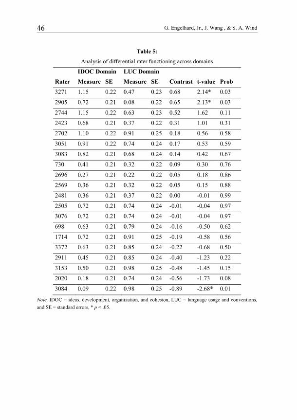
We also included an interaction term (i.e., domain by rater facets) in the model. We used t-tests to compare the differences of accuracy measures between domains for each rater. Results indicate that three raters have significantly different accuracy measures between the two domains (Table 5). Specifically, Raters 3271 and 2905 appear to be significantly more accurate in scoring Domain IDOC than Domain LUC. On the contrary, Rater 3084 seems to be significantly more accurate in Domain LUC than Domain IDOC. In order to interpret these results in terms of their substantive implications, it is informative to relate these results to the five aspects of inaccuracy described in Table 1. Specifically, rater inaccuracy is the tendency on the part of raters to consistently provide higher or lower ratings overall. The illustrative data in this study suggest that the individual raters vary in their levels of inaccuracy. The Wright Map (Figure 5) provides a visual display of where each rater is located on the accuracy continuum. The raters are not equivalent in terms of accuracy rates. The data also provide evidence of domain variation in inaccuracy (halo inaccuracy). Some raters appear to vary in their accuracy rates as a function of do-main. Overall, there were differences in rater accuracy between the two domains, where the IDOC domain was more difficult for raters to score accurately as compared to the LUC domain. Next, response set inaccuracy implies that a rater interprets and uses rating scale categories in an idiosyncratic fashion. Because the accuracy data in this study are dichotomous, this issue is moot. Third, score range inaccuracy is observed in these data with the benchmark essays varying in difficulty to rate accurately as shown on the Wright Map (Figure 5). Further research is needed on why certain essays appear to be more accurately rated than other essays. Finally, there was evidence of an inaccuracy interaction effect between raters and domains. This result suggests that rater effects are not additive, and that the domain facet is not invariant across raters. In other words, the relative ordering of the domains in terms of the difficulty to assign accurate ratings was not the same for all of the raters.
G. Engelhard, Jr., J. Wang , & S. A. Wind 46
Table 5:
Analysis of differential rater functioning across domains
IDOC Domain LUC Domain Rater Measure SE Measure SE Contrast t-value Prob 3271 1.15 0.22 0.47 0.23 0.68 2.14* 0.03
2905 0.72 0.21 0.08 0.22 0.65 2.13* 0.03
2744 1.15 0.22 0.63 0.23 0.52 1.62 0.11
2423 0.68 0.21 0.37 0.22 0.31 1.01 0.31
2702 1.10 0.22 0.91 0.25 0.18 0.56 0.58
3051 0.91 0.22 0.74 0.24 0.17 0.53 0.59
3083 0.82 0.21 0.68 0.24 0.14 0.42 0.67
730 0.41 0.21 0.32 0.22 0.09 0.30 0.76
2696 0.27 0.21 0.22 0.22 0.05 0.18 0.86
2569 0.36 0.21 0.32 0.22 0.05 0.15 0.88
2481 0.36 0.21 0.37 0.22 0.00 -0.01 0.99
2505 0.72 0.21 0.74 0.24 -0.01 -0.04 0.97
3076 0.72 0.21 0.74 0.24 -0.01 -0.04 0.97
698 0.63 0.21 0.79 0.24 -0.16 -0.50 0.62
1714 0.72 0.21 0.91 0.25 -0.19 -0.58 0.56
3372 0.63 0.21 0.85 0.24 -0.22 -0.68 0.50
2911 0.45 0.21 0.85 0.24 -0.40 -1.23 0.22
3153 0.50 0.21 0.98 0.25 -0.48 -1.45 0.15
2020 0.18 0.21 0.74 0.24 -0.56 -1.73 0.08
3084 0.09 0.22 0.98 0.25 -0.89 -2.68* 0.01
Note. IDOC = ideas, development, organization, and cohesion, LUC = language usage and conventions, and SE = standard errors, * p < .05.
A tale of two models 47
+-----------------------------------------------------+ |Logit|+Rater |-Essay |-Domains| |-----+--------------------------+-----------+--------|
High Accuracy Hard Hard | 2 + + + | | | | | | | | | | | | | | | | | | | | | | | | * | | | | | | | | | | * | | | | | ***** | | | | | | | | 1 + 2702 + + | | | 2744 | **** | | | | 1714 3051 3083 3271 | ***** | | | | 698 2505 3076 3153 3372 | ****** | | | | 2911 | ** | | | | 2423 3084 | ***** | | | | 730 2020 2481 2905 | **** | IDOC | | | 2569 | *** | | | | 2696 | ********* | | | | | ******** | | * 0 * * ****** * * | | | ** | | | | | | | | | | ******** | | | | | ****** | LUC | | | | *** | | | | | | | | | | ******* | | | | | ****** | | | | | | | | -1 + + *** + | | | | | | | | | | | | | | | | | | | ** | | | | | | | | | | | | | | | * | | | | | | | | | | | | | -2 + + *** + |
Low Accuracy Easy Easy |-----+--------------------------+-----------+--------|
Note. IDOC = ideas, development, organization, and cohesion, LUC = language usage and conventions.
Figure 5:
Wright Map for Rater Accuracy Model
Discussion
In this study, we briefly discussed two perspectives on evaluating the quality of ratings in rater-mediated assessments: a psychometric perspective and a cognitive perspective. As shown in Figure 1, rater-mediated assessments rely on both perspectives to have reliable, valid, and fair ratings in a rater-mediated assessment system of performances. Much of the current research on rating quality has been dominated by a psychometric perspective with relatively little research on the cognitive processes of human raters. In order to meaning-fully evaluate and interpret the quality of ratings, it is important to explicitly consider both
G. Engelhard, Jr., J. Wang , & S. A. Wind 48
theory of measurement and theory of rater cognition. Ideally, these two perspectives should be complementary and congruent. The psychometric perspective used in this study is based on Rasch measurement theory, and the cognitive perspective is based on Brunswik's lens model. In particular, we emphasized the use of a rater accuracy model (RAM) to illustrate our major points. Our study was guided by the following three questions:
• What psychometric perspectives can be used to evaluate ratings in rater-mediated assessments?
• What cognitive perspectives can provide guidance on how to model judgments obtained in rater-mediated assessments?
• How can we connect these two theoretical perspectives to improve rater-medi-ated assessments?
In answer to the first question, we believe that a scaling perspective based on item response theory in general and Rasch measurement theory in particular provides the best match to the models of judgment in rater-mediated assessments. Rasch measurement theory speci-fies the requirements necessary for developing and maintaining a psychometrically sound performance assessment system. There are two versions of the Rasch model that can be used to evaluate rater accuracy. A Rasch model with observed ratings and a Rasch model with accuracy ratings which is called Rater Accuracy Model. The first model focuses on two assessment systems (one based on expert raters and the second on operational raters) with the latent variable defining the object of measurement for both groups of raters. The second model (i.e., RAM) focuses on rater accuracy directly as the latent variable with the raters defined as the objects of measurement. RAM offers a direct evaluation of rater ac-curacy measures with accuracy ratings which are defined as the differences between ob-served and criterion ratings. Turning now to the second question, we selected cognitive perspectives based on Brunswik's Lens Model as the basis for examining human judgments in rater-mediated assessments. Lens models connect the criterion system and the judgmental system which can best represent operational raters’ cognition processes while making judgments. We have described two lens models. Lens Model I is for measuring student proficiency (e.g., writing competency) as the distal variable (Figure 3). Lens Model II is for measuring rater accuracy directly as the distal variable (Figure 4), which emphasizes the evaluation of the raters or judges by modeling the distances between operational ratings and criterion rat-ings. The final question raises an important issue about the congruence between a statistical theory of measurement and a substantive theory regarding human cognition and judgment. Lens models can be conceptually linked to both the Many-Facet Rasch Model and the RAM with the major distinctions between the objects of measurement in two models. For both models, it is substantively useful to visualize the locations of the object of measure-ment on a Wright Map, to define the latent variable in terms of the specific cues used by the raters as lens, and to conceptualize two systems -- criterion system and judgmental system. The Many-Facet Rasch Model analyzes the two systems separately and then

A tale of two models 49
compares the results. The measurement focuses on student proficiency as a latent contin-uum in each system, and the consistency between two systems reflects the rater accuracy. On the other hand, the RAM is used to model accuracy ratings defined as the distances between the two systems. This approach directly reflects rater accuracy by modeling it as the underlying latent trait. Using illustrative data from a rater-mediated writing performance assessment, we demon-strated the statistical procedures for modeling rater accuracy. Specifically, we calculated accuracy ratings by matching operational ratings and the criterion ratings for individual raters. Then we used the RAM to analyze accuracy ratings to obtain the accuracy measures for individual raters, the difficulty associated with scoring accuracy for student perfor-mances (i.e., essays), and the difficulty associated with scoring accuracy for the domains that were specified in the analytic scoring rubric. To evaluate differential rater functioning, we examined the interaction between individual raters and domains. Lastly, we interpreted the statistical results of RAM based on the five potential sources of inaccuracy. These sources of inaccuracy also provide a frame of reference for interpreting the statistical re-sults in terms of specific rater issues in operational performance assessments. We want to stress that the statistical theories of measurement and substantive theories of human cognition and judgment for evaluating rating quality should be complementary and congruent. Ideally, research on rater-mediated assessments should balance concerns with both cognitive and psychometric perspectives. In practice, the development and evaluation of how well our theories match one another remains a challenging puzzle. As progress is made in both areas, the nexus between psychometrics and cognition for rater-mediated assessments promises to be an exciting area of research. Finally, the title of this study reflects an indirect reference to the opening lines in A Tale of Two Cities (Charles Dickens, 1859):
It was the best of times, it was the worst of times, it was the age of wisdom, it was the age of foolishness, it was the epoch of belief, it was the epoch of incredulity, it was the season of Light, it was the season of Darkness, it was the spring of hope, it was the winter of despair…
Some researchers who evaluate rater-mediated assessments have numerous justifiable con-cerns about human biases and errors (e.g., intentional and random), and their perspectives may reflect despair over the current state of the art. From our perspective, we have hope that many of the concerns about human scoring can be minimized and the promise of per-formance assessments become a reality in education and other contexts. In particular, we believe that explicit considerations of both psychometric and cognitive perspectives have important implications for improving the training and maintaining the quality of ratings obtained from human raters in performance assessments.
References
Andrich, D. (1978). A rating formulation for ordered response categories. Psychometrika, 43, 561-73.
G. Engelhard, Jr., J. Wang , & S. A. Wind 50
Athanasou, J.A., & Kaufmann, E. (2015). Probability of responding: A return to the original Brunswik. Psychological Thought, 8(1), 7–16.
Barsalou, L. W. (1992). Cognitive psychology: An overview for cognitive scientists. Psychology Press.
Bergin, C., Wind, S. A., Grajeda, S., & Tsai, C.-L. (2017). Teacher evaluation: Are principals' classroom observations accurate at the conclusion of training? Studies in Educational Eval-uation, 55, 19–26.
Brunswik, E. (1952). The conceptual framework of psychology. Chicago, IL: University of Chi-cago Press.
Brunswik, E. (1955a). Representative design and probabilistic theory in a functional psychol-ogy. Psychological Review, 62(3), 193-217.
Brunswik, E. (1955b). In defense of probabilistic functionalism: A reply. Psychological Re-view, 62(3), 236-242.
Brunswik, E. (1956). Perception and the representative design of psychological experiments (2nd ed.). Berkeley, CA: University of California Press.
Casabianca, J. M., Junker, B. W., & Patz, R. J. (2016). Hierarchical rater models. In W. J. van der Linden (Ed.), Handbook of item response theory (Vol. 1, pp. 449–465). Boca Raton, FL: Chapman & Hall/CRC.
Cooksey, R. W. (1996). Judgment analysis: Theory, methods, and applications. United King-dom: Emerald Group Publishing Limited.
Cooksey, R. W., Freebody, P., & Davidson, G. R. (1986). Teachers' predictions of children's early reading achievement: An application of social judgment theory. American Educatio-nal Research Journal, 23(1), 41-64.
Cooksey, R. W., Freebody, P., & Wyatt-Smith, C. (2007). Assessment as judgment-in-context: Analysing how teachers evaluate students' writing. Educational Research and Evaluation, 13(5), 401-434.
Cronbach, L. J., Gleser, G. C., Nanda, H., & Rajaratnam, N. (1972). The dependability of be-havioral measurements: Theory of generalizability for scores and profiles. New York: Wiley.
Dickens, C. J. H. (1859). A tale of two cities (Vol. 1). Chapman and Hall. Eckes, T. (2005). Examining rater effects in TestDaF writing and speaking performance assess-
ments: A many-facet Rasch analysis. Language Assessment Quarterly, 2(3), 197–221.
Eckes, T. (2015). Introduction to many-facet Rasch measurement: Analyzing and evaluating rater mediated assessments (2nd ed.). Frankfurt am Main: Peter Lang.
Engelhard Jr, G. (1992). The measurement of writing ability with a many-faceted Rasch model. Applied Measurement in Education, 5(3), 171-191.
Engelhard, G. (1994). Examining rater errors in the assessment of written composition with a many-faceted Rasch model. Journal of Educational Measurement, 31(2), 93-112.
Engelhard, G. (1996). Evaluating rater accuracy in performance assessments. Journal of Edu-cational Measurement, 33(1), 56-70.

A tale of two models 51
Engelhard, G. (2002). Monitoring raters in performance assessments. In G. Tindal and T. Hala-dyna (Eds.), Large-scale assessment programs for ALL students: Development, implemen-tation, and analysis, (pp. 261-287). Mahwah, NJ: Erlbaum.
Engelhard, G. (2013). Invariant measurement: Using Rasch models in the social, behavioral, and health sciences. New York: Routledge.
Engelhard, G., & Myford, C. (2010). Comparison of single and double assessor scoring designs for the assessment of accomplished teaching. In Garner, M., Engelhard, G., Wilson, M., & Fisher, W. (Eds.). Advances in Rasch measurement (Vol. 1, pp. 342-368). Maple Grove, MN: JAM Press.
Engelhard, G., & Wind, S.A. (2013). Rating quality studies using Rasch measurement theory. College Board Research Report 2013-3.
Guilford, J. P. (1936). Psychometric methods. New York: McGraw Hill. Hammond, K. R. (1955). Probabilistic functioning and the clinical method. Psychological re-
view, 62(4), 255.
Hammond, K. R. (1996). Upon reflection. Thinking & Reasoning, 2(2-3), 239-248. Hammond, K. R., Hursch, C. J., & Todd, F. J. (1964). Analyzing the components of clinical
inference. Psychological review, 71(6), 438. Hursch, C. J., Hammond, K. R., & Hursch, J. L. (1964). Some methodological considerations
in multiple-cue probability studies. Psychological review, 71(1), 42.
Johnson, R. L., Penny, J. A., & Gordon, B. (2009). Assessing performance: Designing, scoring, and validating performance tasks. New York: Guilford Press.
Karelaia, N., & Hogarth, R.M. (2008). Determinants of linear judgment: A meta-analysis of lens model studies. Psychological Bulletin, 134(3), 404–426.
Kaufmann, E., Reips, U. D., & Wittmann, W. W. (2013). A critical meta-analysis of lens model studies in human judgment and decision-making. PloS one, 8(12), e83528.
Kendall, M. G., & Buckland, W. R. (1957). Dictionary of statistical terms. Edinburgh, Scot-land: Oliver and Boyd.
Lane, S. (2016). Performance assessment and accountability: Then and now. In C. Wells & M. Faulkner-Bond (Eds). Educational measurement: From foundations to future (pp. 356-372). New York: Guilford.
Leighton, J. P. (2012). Editorial. Educational Measurement: Issues & Practice, 31(3), 48-49.
Linacre, J. M. (1989). Many-facet Rasch measurement. Chicago, IL: MESA Press. Linacre, J. M. (2015) Facets computer program for many-facet Rasch measurement, version
3.71.4. Beaverton, Oregon: Winsteps.com Masters, G. N. (1982). A Rasch model for partial credit scoring. Psychometrika, 47(2), 149-
174.
Muraki, E. (1992). A generalized partial credit model: Application of an EM algorithm. Applied Psychological Measurement, 16, 159–176.
Myford, C. M. (2012). Rater cognition research: Some possible directions for the future. Edu-cational Measurement: Issues & Practice, 31(3), 48-49.

G. Engelhard, Jr., J. Wang , & S. A. Wind 52
Nering, M.L., & Ostini, R. (2010). Handbook of polytomous item response theory models. New York: Routledge.
Patterson, B.F., Wind, S.A., & Engelhard, G. (2017). Incorporating criterion ratings into model-based rater monitoring procedures using latent class signal detection theory. Applied Psy-chological Measurement, 1-20.
Postman, L., & Tolman, E. C. (1959). Brunswik's probabilistic functionalism. Psychology: A study of a science, 1, 502-564.
Rasch (1960/1980). Probabilistic models for some intelligence and attainment tests. Copenha-gen: Danish Institute for Educational Research. (Expanded edition, Chicago: University of Chicago Press, 1980).
Samejima, F. (1969). Estimation of latent ability using a response pattern of graded scores. Psychometrika Monograph, No. 17.
Tucker, L. R. (1964). A suggested alternative formulation in the developments by Hursch, Ham-mond, and Hursch, and by Hammond, Hursch, and Todd. Psychological Review, 71(6), 528-530.
von Eye, A., & Mun E. Y. (2005). Analyzing rater agreement: Manifest variable methods. Mahwah, NJ: Erlbaum.
Wang, J., Engelhard, G., & Wolfe, E. W. (2016). Evaluating rater accuracy in rater-mediated assessments with an unfolding model. Educational and Psychological Measurement, 76, 1005–1025.
Wang, J., Engelhard, G., Raczynski, K., Song, T., & Wolfe, E. W. (2017). Evaluating rater accuracy and perception for integrated writing assessments using a mixed-methods ap-proach. Assessing Writing, 33, 36-47.
Wesolowski, B. W., & Wind, S. A. (in press). Investigating rater accuracy in the context of secondary-level solo instrumental music. Musicae Scientae.
Wesolowski, B., Wind, S.A., & Engelhard, G. (2016). Examining rater precision in music per-formance assessment: An analysis of rating scale structure using the multifaceted Rasch partial credit model. Music Perception, 33(5), 662–678.
Wind, S.A., & Engelhard, G. (2013). How invariant and accurate are domain ratings in writing assessment? Assessing Writing, 18, 278–299.
Wolfe, E. W. (2014). Methods for monitoring rating quality: Current practices and suggested changes. Iowa City, IA: Pearson.
Wolfe, E. W., Jiao, H., & Song, T. (2014). A family of rater accuracy models. Journal of Ap-plied Measurement, 16(2), 153-160.
Wolfe, E. W., & McVay, A. (2012). Application of latent trait models to identifying substan-tively interesting raters. Educational Measurement: Issues and Practice, 31(3), 31–37.
Wang, J. & Engelhard, G. (2017). Using a multifocal lens model and Rasch measurement theory to evaluate rating quality in writing assessments. Pensamiento Educativo: Journal of Latin-American Educational Research, 54(2), 1-16.
Wind, S. A., & Peterson, M. E. (2017). A systematic review of methods for evaluating rating quality in language assessment. Language Testing, doi: 10.1177/0265532216686999

Psychological Test and Assessment Modeling, Volume 60, 2018 (1), 53-80
Modeling rater effects using a combination
of Generalizability Theory and IRT
Jinnie Choi1 & Mark R. Wilson
2
Abstract
Motivated by papers on approaches to combine generalizability theory (GT) and item response
theory (IRT), we suggest an approach that extends previous research to more complex measure-
ment situations, such as those with multiple human raters. The proposed model is a logistic mixed
model that contains the variance components needed for the multivariate generalizability coeffi-
cients. Once properly set-up, we can estimate the model by straightforward maximum likelihood
estimation. We illustrate the use of the proposed method with a real multidimensional polytomous
item response data set from classroom assessment that involved multiple human raters in scoring.
Keywords: generalizability theory, item response theory, rater effect, generalized linear mixed
model
1Correspondence concerning this article should be addressed to: Jinnie Choi, Research Scientist at
Pearson, 221 River Street, Hoboken, NJ 07030; email: [email protected]. 2University of California, Berkeley

J. Choi & M.R. Wilson 54
While item response theory (IRT; Lord, 1980; Rasch, 1960) and generalizability theory
(GT; Brennan, 2001; Cronbach, Gleser, Nanda, & Rajaratnam, 1972) share common
goals in educational and psychological research in order to provide evidence of the quali-
ty of measurement, IRT and GT have evolved into two separate domains of knowledge
and practice in psychometrics that rarely communicate with one another. In practice, it is
often recommended that researchers and practitioners be able to use and understand both
methods, and to distinguish the same term with different meanings (e.g., reliability) or
different terms with similar meanings (e.g., unidimensional testlet design in IRT and p x
(i : h) design in GT), neither of which is desirable or practical. The separate foundations
and development of these two techniques have resulted in a wide gap between the two
approaches and have hampered collaboration between those who specialize in each.
Additionally, despite the theories’ extensive applicability, IRT and GT are often applied
to somewhat different areas of research and practice. For example, applications of GT
are often found in studies on reliability and sampling variability of smaller-scale assess-
ments. Meanwhile, IRT is, relatively speaking, more commonly and more widely em-
ployed, than GT for developing large-scale educational assessments, such as the Pro-
gramme for International Student Assessment (PISA) and the ones currently used by the
US National Center for Education Statistics (NCES), and the products of large testing
companies such as Educational Testing Service (ETS). Moreover, most advanced appli-
cations of IRT and GT take only one approach, not both. Considering the advantages of
the two theories, this limitation and bias in usage call for an alternative approach to pro-
mote a more efficient and unified way to deliver the information that can be provided by
IRT and GT together.
Several researchers have undertaken efforts to find the solution to this separation. For
example, the researchers either: (a) highlight the differences but suggest using both,
consecutively (Linacre, 1993), (b) discuss the link between the models (Kolen & Harris,
1987; Patz, Junker, Johnson, & Mariano, 2002), or (c) propose a new approach to com-
bine the two (Briggs & Wilson, 2007).
Linacre (1993) emphasized the difference between IRT and GT and suggested that deci-
sion-makers select either one or the other, or use both, based on the purpose of the analy-
sis. Many researchers took this advice and used both the IRT and the GT models, for
example, for performance assessments of English as Second Language students (Lynch
& McNamara, 1998), for English assessment (MacMillan, 2000), for writing assessments
of college sophomores (Sudweeks, Reeve, & Bradshaw, 2005), for problem-solving
assessments (Smith & Kulikowich, 2004), and for clinical examinations (Iramaneerat,
Yudkowsky, Myford, & Downing, 2008).
While Linacre’s suggestion promoted the idea of combining the use of the models, the
statistical notion of links between IRT and GT began to emerge when Kolen and Harris
(1987) proposed a multivariate model based on a combination of IRT and GT. The mod-
el assumed that the true score in GT could be approximated by the proficiency estimate
in IRT. Patz, Junker, Johnson, & Mariano (2002) proposed a new model that combines
IRT and GT, namely, the hierarchical rater model (HRM), which they see as a standard
generalizability theory model for rating data, with IRT distributions replacing the normal
theory true score distributions that are usually implicit in inferential applications of the

Modeling rater effects 55
model. The proposed use of the model is open to other possible extensions, although it is
currently conceptualized as being used for estimation of rater effects.
These efforts motivated a noteworthy advance in combining IRT and GT, namely, the
Generalizability in Item Response Modeling (GIRM) approach by Briggs & Wilson
(2007), and its extensions by Choi, Briggs, & Wilson (2009) and Chien (2008). The
GIRM approach provides a method for estimating traditional IRT parameters, the GT-
comparable variance components, and the generalizability coefficients, not with ob-
served scores but with the “expected item response matrix” — EIRM. By estimating a
crossed random effects IRT model within a Bayesian framework, the GIRM procedure
constructs the EIRM upon which GT-comparable analysis can be conducted. The steps
can be described as follows:
Step 1. The probability of a correct answer is modeled using a crossed random ef-
fects item response model that considers both person and item as random
variables. The model parameters are estimated using the Markov chain
Monte Carlo (MCMC) method with the Gibbs sampler.
Step 2. Using the estimates from Step 1, the probability of the correct answer for
each examinee answering each item is predicted to build the EIRM.
Step 3. The variance components and generalizability coefficients are estimated
based on the EIRM.
Estimation of the variance components and generalizability coefficients utilizes an ap-
proach described by Kolen and Harris (1987) that calculates marginal integrals for facet
effects, interaction effect, and unexplained error using the prior distributions and the
predicted probabilities of IRT model parameters.
The main findings of the Briggs & Wilson (2007) study were as follows:
GIRM estimates are comparable to GT estimates in the simple p x i test design
where there are person and item facets alone, and with binary data.
GIRM easily deals with the missing data problem, a problem for earlier ap-
proaches, by using the expected response matrix.
Because GIRM combines the output from IRT with the output from GT, GIRM
provides more information than either approach in isolation.
Although GIRM adds the IRT assumptions and distributional assumptions to
the GT sampling assumptions, GIRM is robust to misspecification of item re-
sponse function and prior distributions.
In the multidimensional extension of the same method, Choi, Briggs, and Wilson (2009)
found that the difference between GIRM and traditional GT estimates is more noticeable,
with GIRM producing more stable variance component estimates and generalizability
coefficients than traditional GT. Noticeable patterns of differences included the follow-
ing:
GIRM item variance estimates were smaller and more stable than GT,
J. Choi & M.R. Wilson 56
GIRM error variance (pi + e) estimates were larger and more stable than GT
residual error variance (pie) estimates, and
GIRM generalizability coefficients were generally larger and more precise than
GT generalizability coefficients.
With the testlet extension of the procedure by Chien (2008), (a) the estimates of the
person, the testlet, the interaction between the item and testlet, and the residual error
variance estimates were found to be comparable to traditional GT estimates when data
are generated from IRT models. (b) For the dataset generated from GT models, the inter-
action and residual variance estimates were slightly larger while person variance esti-
mates were slightly smaller than traditional GT estimates. (c) The person-testlet interac-
tion variance estimates were slightly larger than the traditional GT estimates for all con-
ditions. (d) When the sample size was small, the discrepancy between the estimated
universe mean scores in GT and the expected data in GIRM increased. (e) MCMC stand-
ard errors were notably underestimated for all variance components.
The mixed results from the studies of GIRM and its extensions yielded interesting ques-
tions.
What is the statistical nature of the EIRM? The main advantage of the GIRM
procedure comes from this matrix, coupled with the MCMC estimation within a
Bayesian framework. This is a notable departure from the analogous-ANOVA
estimation of traditional GT that brings the following benefits: (a) the variance
component estimates are non-negative and (b) the problems that arise from un-
balanced designs and missing data are easily taken care of. However, the exten-
sion studies revealed that the EIRM does not theoretically guarantee the equiva-
lence of GIRM and traditional GT estimates in more complicated test condi-
tions.
Then, what is the benefit of having the extra step that requires multiple sets of
assumptions and true parameters for each stage?
Are there other ways to deal with the negative variance estimate problem in
traditional GT and the missing data problem, and still get comparable results?
Among the different approaches, which procedure gives more correct esti-
mates?
These questions led to the search for an alternative strategy that requires simple one-
stage modeling, and possibly non-Bayesian estimation that produces GT-comparable
results, while capturing the essence of having random person and item parameters and
variance components. The following section describes a different approach, one within
the GLLAMM framework, to combine GT and IRT. In the next section, we explain how
the random person and item parameters are estimated using a Laplace approximation
implemented in the lmer() function (Bates, Maechler, Bolker, & Walker, 2014) in the R
Statistical Environment (R Development Core Team, 2017). After that, we demonstrate
applications of our approach to classroom assessment data from the 2008-2009 Carbon
Cycle project, which includes 1,371 students’ responses to 19 items, rated by 8 raters.

Modeling rater effects 57
The proposed model
This paper uses a generalized linear latent and mixed model (GLLAMM; Skrondal &
Rabe-Hesketh, 2004; Rabe-Hesketh, Skrondal, & Pickles, 2004) approach as an alterna-
tive to existing efforts to combine GT and IRT. GLLAMM offers a flexible one-stage
modeling framework for a combination of crossed random effects IRT models and GT
variance components models. The model is relatively straight-forward to formulate and
easily expandable to more complex measurement situations such as multidimensionality,
polytomous data, and multiple raters. In this section, we describe how the model speci-
fies a latent threshold parameter as a function of cross-classified person, item, and rater
random effects and the variance components for each facet.
GLLAMM is an extended family of generalized linear mixed models (Breslow & Clay-
ton, 1993; Fahrmeir & Tutz, 2001), which was developed in the spirit of synthesizing a
wide variety of latent variable models used in different academic disciplines. This gen-
eral model framework has three parts. The response model formulates the relationship
between the latent variables and the observed responses via the linear predictor and link
function, which accommodates various kinds of response types. The structural model
specifies the relationship between the latent variables at several levels. Finally, the dis-
tribution of disturbances for the latent variables is specified. For more details, see Rabe-
Hesketh et al. (2004) and Skrondal & Rabe-Hesketh (2004). In this section, GT and IRT
are introduced as special case of GLLAMM. Then, the GLLAMM approach to combin-
ing GT and IRT is detailed.
GT in the GLLAMM framework
The GLLAMM framework for traditional GT models consists of the response model for
continuous responses, and multiple levels of crossing between latent variables. A multi-
faceted measurement design with person, item and rater facets will be used for an exam-
ple. First, suppose, for the moment, that there is a continuous observed score for person j
on item i rated by rater k which is modeled as
𝑦𝑖𝑗𝑘 = 𝜈𝑖𝑗𝑘 + 𝜖𝑖𝑗𝑘, (1)
Where the error 𝜖𝑖𝑗𝑘 has variance 𝜎 and the linear predictor 𝜈𝑖𝑗𝑘 is defined as a three-way
random effects model
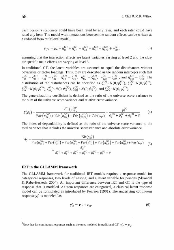
𝜈𝑖𝑗𝑘 = 𝛽0 + 𝜂1𝑖(2)
+ 𝜂2𝑗(2)
+ 𝜂3𝑘(2)
, (2)
where 𝛽0 is the grand mean in the universe of admissible observations. 𝜂1𝑖(2)
, 𝜂2𝑗(2)
, and
𝜂3𝑘(2)
are interpreted as item, person, and rater effects, respectively. The (2) superscript
denotes that the units of the variable vary at level 2. The subscript starts with a number
identifier for latent variables and the alphabetical identifier for units. These effects are
not considered nested but crossed because each person could have answered any item,
J. Choi & M.R. Wilson 58
each person’s responses could have been rated by any rater, and each rater could have
rated any item. The model with interactions between the random effects can be written as
a reduced form multilevel model,
𝜈𝑖𝑗𝑘 = 𝛽0 + 𝜂1𝑖(3)
+ 𝜂2𝑗(3)
+ 𝜂3𝑘(3)
+ 𝜂4𝑖𝑗(2)
+ 𝜂5𝑗𝑘(2)
+ 𝜂6𝑖𝑘(2)
, (3)
assuming that the interaction effects are latent variables varying at level 2 and the clus-
ter-specific main effects are varying at level 3.
In traditional GT, the latent variables are assumed to equal the disturbances without
covariates or factor loadings. Thus, they are described as the random intercepts such that
𝜂1𝑖(3)
= 𝜁1𝑖(3)
, 𝜂2𝑗(3)
= 𝜁2𝑗(3)
, 𝜂3𝑘(3)
= 𝜁3𝑘(3)
, 𝜂1𝑖𝑗(2)
= 𝜁1𝑖𝑗(2)
, 𝜂2𝑗𝑘(2)
= 𝜁2𝑗𝑘(2)
, and 𝜂3𝑖𝑘(2)
= 𝜁3𝑖𝑘(2)
. The
distribution of the disturbances can be specified as 𝜁1𝑖(3)
~𝑁(0, 𝜓1(3)
), 𝜁2𝑗(3)
~𝑁(0, 𝜓2(3)
),
𝜁3𝑘(3)
~𝑁(0, 𝜓3(3)
), 𝜁4𝑖𝑗(2)
~𝑁(0, 𝜓4(2)
), 𝜁5𝑗𝑘(2)
~𝑁(0, 𝜓5(2)
), and 𝜁6𝑖𝑘(2)
~𝑁(0, 𝜓6(2)
).
The generalizability coefficient is defined as the ratio of the universe score variance to
the sum of the universe score variance and relative error variance.
𝐸(�̂�𝐽2) =
𝑉𝑎�̂�(𝜂2𝑗(3)
)
𝑉𝑎�̂� (𝜂2𝑗
(3)) + 𝑉𝑎�̂� (𝜂4𝑖𝑗
(2)) + 𝑉𝑎�̂� (𝜂5𝑗𝑘
(2)) + 𝑉𝑎�̂�(𝜖𝑖𝑗𝑘)
=�̂�2
(3)
�̂�2(3)
+ �̂�4(2)
+ �̂�5(2)
+ �̂� (4)
The index of dependability is defined as the ratio of the universe score variance to the
total variance that includes the universe score variance and absolute error variance.
𝛷�̂� =𝑉𝑎�̂�(𝜂2𝑗
(3))
𝑉𝑎�̂�(𝜂1𝑖
(3)) + 𝑉𝑎�̂�(𝜂2𝑗
(3)) + 𝑉𝑎�̂�(𝜂3𝑘
(3)) + 𝑉𝑎�̂�(𝜂4𝑖𝑗
(2)) + 𝑉𝑎�̂�(𝜂5𝑗𝑘
(2)) + 𝑉𝑎�̂�(𝜂6𝑖𝑘
(2)) + 𝑉𝑎�̂�(𝜖𝑖𝑗𝑘)
=�̂�2
(3)
�̂�1(3)
+ �̂�2(3)
+ �̂�3(3)
+ �̂�4(2)
+ �̂�5(2)
+ �̂�6(2)
+ �̂�
(5)
IRT in the GLLAMM framework
The GLLAMM framework for traditional IRT models requires a response model for
categorical responses, two levels of nesting, and a latent variable for persons (Skrondal
& Rabe-Hesketh, 2004). An important difference between IRT and GT is the type of
response that is modeled. As item responses are categorical, a classical latent response
model can be formulated as introduced by Pearson (1901). The underlying continuous
response 𝑦𝑖𝑗∗ is modeled
3 as
𝑦𝑖𝑗∗ = 𝜈𝑖𝑗 + 𝜖𝑖𝑗 . (6)
3Note that for continuous responses such as the ones modeled in traditional GT, 𝑦𝑖𝑗
∗ = 𝑦𝑖𝑗.
Modeling rater effects 59
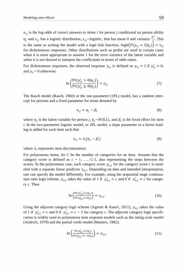
𝜈𝑖𝑗 is the log odds of correct answers to items i for person j conditional on person ability
𝜂𝑗 and 𝜖𝑖𝑗 has a logistic distribution, 𝜖𝑖𝑗~logistic, that has mean 0 and variance 𝜋2
3. This
is the same as writing the model with a logit link function, logit(𝑃(𝑦𝑖𝑗 = 1|𝜂𝑗)) = 𝜈𝑖𝑗
for dichotomous responses. Other distributions such as probit are used in certain cases
when it is more appropriate to assume 1 for the error variance of the latent variable and
when it is not desired to interpret the coefficients in terms of odds ratios.
For dichotomous responses, the observed response 𝑦𝑖𝑗 is defined as 𝑦𝑖𝑗 = 1 if 𝑦𝑖𝑗∗ > 0,
and yij = 0 otherwise.
ln (Pr (𝑦𝑖𝑗
∗ > 0|𝜂𝑗)
Pr (𝑦𝑖𝑗∗ ≤ 0|𝜂𝑗)
) = 𝜈𝑖𝑗 (7)
The Rasch model (Rasch, 1960) or the one-parameter (1PL) model, has a random inter-
cept for persons and a fixed parameter for items denoted by
𝜈𝑖𝑗 = 𝜂𝑗 − 𝛽𝑖 (8)
where 𝜂𝑗 is the latent variable for person j, 𝜂𝑗~𝑁(0,1), and 𝛽𝑖 is the fixed effect for item
i. In the two-parameter logistic model, or 2PL model, a slope parameter or a factor load-
ing is added for each item such that
𝜈𝑖𝑗 = 𝜆𝑖(𝜂𝑗 − 𝛽𝑖) (9)
where 𝜆𝑖 represents item discrimination.
For polytomous items, let C be the number of categories for an item. Assume that the
category score is defined as c = 1, …, C-1, also representing the steps between the
scores. In the polytomous case, each category score 𝑦𝑖𝑐𝑗 for the category score c is mod-
eled with a separate linear predictor 𝜈𝑖𝑐𝑗 . Depending on data and intended interpretation,
one can specify the model differently. For example, using the sequential stage continua-
tion ratio logit scheme, 𝑦𝑖𝑐𝑗 takes the value of 1 if 𝑦𝑖𝑐𝑗∗ > 𝑐 and 0 if 𝑦𝑖𝑐𝑗
∗ = 𝑐 for catego-
ry c. Then
ln (Pr (𝑦𝑖𝑐𝑗
∗ >𝑐|𝜂𝑗)
Pr (𝑦𝑖𝑐𝑗∗ =𝑐|𝜂𝑗)
) = 𝜈𝑖𝑐𝑗. (10)
Using the adjacent category logit scheme (Agresti & Kateri, 2011), 𝑦𝑖𝑐𝑗 takes the value
of 1 if 𝑦𝑖𝑐𝑗∗ = 𝑐 and 0 if 𝑦𝑖𝑐𝑗
∗ = 𝑐 − 1 for category c. The adjacent category logit specifi-
cation is widely used in polytomous item response models such as the rating scale model
(Andrich, 1978) and the partial credit model (Masters, 1982):
ln (Pr (𝑦𝑖𝑐𝑗
∗ =𝑐|𝜂𝑗)
Pr (𝑦𝑖𝑐𝑗∗ =𝑐−1|𝜂𝑗)
) = 𝜈𝑖𝑐𝑗 . (11)

J. Choi & M.R. Wilson 60
In cumulative models for ordered categories, 𝑦𝑖𝑐𝑗 takes the value of 1 if 𝑦𝑖𝑐𝑗∗ > 𝑐 and 0 if
𝑦𝑖𝑐𝑗∗ ≤ 𝑐 for category c. The graded response model (Samejima, 1969) is specified using
cumulative probabilities and threshold parameters. When a logit link is used, the model
is specified as,
ln (Pr (𝑦𝑖𝑐𝑗
∗ >𝑐|𝜂𝑗)
Pr (𝑦𝑖𝑐𝑗∗ ≤𝑐|𝜂𝑗)
) = 𝜈𝑖𝑐𝑗. (12)
In the case of the partial credit model, the linear predictor is specified as
𝜈𝑖𝑐𝑗 = 𝑐𝜂𝑗 − 𝛽𝑖𝑐 (13)
with 𝛽𝑖𝑐 representing the cth step difficulty for item i. The graded response model uses a
set of ordered threshold parameters 𝜅𝑐 such that
𝜈𝑖𝑐𝑗 = 𝜅𝑐𝜂𝑗 − 𝛽𝑖𝑐 (14)
where 𝜅𝑐 can be viewed as the factor loadings for each step.
Zheng & Rabe-Hesketh (2007) presented the Rasch, 2PL, partial credit model and rating
scale model using the additional parameters for covariates for latent variables and other
parameters, so that the structure of item loading and scoring is more explicit.
Theoretical link and justification of combining GT and IRT using GLLAMM
The combination of GT and IRT ideas become simpler when GT and IRT features are
expressed in the same GLLAMM language. The key elements of the combined model
include: the latent response specification, a logit link, and a linear predictor specified as a
crossed random effects model.
For dichotomous responses, the underlying continuous response to the ith item of the j
th
person rated by the kth rater is modeled using a classical latent response model:
𝑦𝑖𝑗𝑘∗ = 𝜈𝑖𝑗𝑘 + 𝜖𝑖𝑗𝑘, 𝜖𝑖𝑗𝑘~𝑙𝑜𝑔𝑖𝑠𝑡𝑖𝑐(𝜇,
𝜋2
3), (15)
where 𝜈𝑖𝑗𝑘 designates the true score for every possible pair of units i, j, and k, or the
expected responses. The observed response 𝑦𝑖𝑗𝑘 is modeled as a threshold that takes the
value of 1 if 𝑦𝑖𝑗𝑘∗ > 0 and 0 otherwise.
The linear predictor 𝜈𝑖𝑗𝑘 is defined as a crossed random effects model with or without
interaction. For simplicity, a model without interaction is presented here as
𝜈𝑖𝑗𝑘 = 𝛽0 + 𝜂1𝑖(2)
+ 𝜂2𝑗(2)
+ 𝜂3𝑘(2)
(16)

Modeling rater effects 61
where 𝛽0 is the average logit of the probability of response 1 averaging over all persons,
items, and raters. Note that the effects for persons and items are not considered nested
but crossed because each person could have answered each item. As above, the (2) su-
perscript denotes that the units of the variable vary at level 2. 𝜂1𝑖(2)
is the first latent varia-
ble that varies among items (i = 1,…,I) at level 2, and 𝜂2𝑗(2)
is the second latent variable at
level 2 that varies among persons (j = 1, …, J). 𝜂3𝑘(2)
is the third latent variable at level 2
that varies among raters (k = 1, …, K). The interpretations of 𝜂1𝑖(2)
, 𝜂2𝑗(2)
, and 𝜂3𝑘(2)
are item
easiness, person ability, and rater leniency, respectively. If the addition signs are
switched to subtraction signs for 𝜂1𝑖(2)
and 𝜂3𝑘(2)
, the interpretations are also reversed as
item difficulty and rater severity.
The latent variables are assumed to equal the disturbances, 𝜂1𝑖(2)
= 𝜁1𝑖(2)
, 𝜂2𝑗(2)
= 𝜁2𝑗(2)
and
𝜂3𝑘(2)
= 𝜁3𝑘(2)
, which are specified as 𝜁1𝑖(2)
~𝑁(0, 𝜓1(2)
), 𝜁2𝑗(2)
~𝑁(0, 𝜓2(2)
), and
𝜁3𝑘(2)
~𝑁(0, 𝜓3(2)
), corresponding to the assumptions of traditional GT.
In the case of person-specific unobserved heterogeneity, the model is specified as
𝜈𝑖𝑗𝑘 = 𝛽0 + 𝜂1𝑖(2)
+ ∑ 𝜆𝑖𝑑𝜂2𝑗𝑑(2)
+ 𝜂3𝑘(2)𝐷
𝑑=1 , 𝜁2𝑗𝑑(2)
~𝑀𝑉𝑁(𝟎, 𝚿2(2)
). (17)
with the number of dimensions D, the item factor loadings 𝜆𝑖𝑑, and a covariance matrix
𝚿. For the Rasch model, 𝜆𝑖𝑑 is 1 if the ith item maps onto the d
th dimension, 0 otherwise.
The continuation ratio approach is used for polytomous data, following Tutz’s (1990)
parameterization in his sequential stage modeling (De Boeck, Bakker, Zwitser, Nivard,
Hofman, Tuerlinckx, & Partchev, 2011). 𝑦𝑖𝑐𝑗𝑘 takes the value of 1 if 𝑦𝑖𝑐𝑗𝑘∗ > 𝑐 and 0 if
𝑦𝑖𝑐𝑗𝑘∗ = 𝑐, where c (c = 1, …, C–1) denotes the category score and C denotes the number
of score categories including the score 0. The linear predictors 𝜈𝑖𝑐𝑗𝑘 for unidimensional
and multidimensional cases are specified as
𝜈𝑖𝑐𝑗𝑘 = 𝛽0 + 𝜂1𝑖𝑐(2)
+ 𝜂2𝑗(2)
+ 𝜂3𝑘(2)
, (18)
𝜈𝑖𝑐𝑗𝑑𝑘 = 𝛽0 + 𝜂1𝑖𝑐(2)
+ ∑ 𝜆𝑖𝑑𝜂2𝑗𝑑(2)
+ 𝜂3𝑘(2)
𝐷
𝑑=1
, 𝜁2𝑗𝑑(2)
~𝑀𝑉𝑁(𝟎, 𝚿2(2)
). (19)
Using the variance components estimates, the generalizability coefficient 𝐸(�̂�𝐽2) for the
person estimates is calculated. In GT terms, 𝐸(�̂�𝐽2) is the ratio of the universe score
variance to the sum of itself plus the relative error variance. The universe score variance
is defined as the variance of all the scores in the population of all the persons, items, and
raters. The relative error variance means the measurement error variance relevant to the
relative rank order between persons. The variance of 𝜖𝑖𝑗𝑘 is included in the denominator
to take into account the variance of the underlying logit. Additionally, using the variance

J. Choi & M.R. Wilson 62
component for items and raters in the model, we calculate the generalizability coefficient
for measurement of item easiness, 𝐸(�̂�𝐼2), and rater leniency, 𝐸(�̂�𝐾
2 ), in the same manner:
𝐸(�̂�𝐽2) =
𝑉𝑎�̂�(𝜂2𝑗(2)
)
𝑉𝑎�̂�(𝜂2𝑗
(2)) + 𝑉𝑎�̂�(𝜖𝑖𝑗𝑘)
=�̂�2
(2)
�̂�2(2)
+𝜋2
3
(20)
𝐸(�̂�𝐼2) =
𝑉𝑎�̂�(𝜂1𝑖(2)
)
𝑉𝑎�̂�(𝜂1𝑖
(2)) + 𝑉𝑎�̂�(𝜖𝑖𝑗𝑘)
=�̂�1
(2)
�̂�1(2)
+𝜋2
3
(21)
𝐸(�̂�𝐾2 ) =
𝑉𝑎�̂�(𝜂3𝑘(2)
)
𝑉𝑎�̂�(𝜂3𝑘
(2)) + 𝑉𝑎�̂�(𝜖𝑖𝑗𝑘)
=�̂�3
(2)
�̂�3(2)
+𝜋2
3
(22)
The index of dependability Φ̂ is the ratio of the universe score variance to the sum of
itself plus the absolute error variance. Absolute error variance focuses on the measure-
ment error variance of a person that is attributed by the measurement facets regardless of
how other people do on the test. Thus, Φ̂ accounts for the variance related to another
random facet, for example, items. The denominator also includes the variance of the
underlying logit. The same logic can be extended to calculation of the indices of depend-
ability for item easiness and rater leniency:
𝛷�̂� =�̂�2
(2)
�̂�1(2)
+ �̂�2(2)
+ �̂�3(2)
+𝜋2
3
(23)
𝛷�̂� =�̂�1
(2)
�̂�1(2)
+ �̂�2(2)
+ �̂�3(2)
+𝜋2
3
(24)
𝛷�̂� =φ̂3
(2)
φ̂1(2)
+ φ̂2(2)
+ �̂�3(2)
+π2
3
(25)
In the multidimensional and/or polytomous case, we use the dimension- and category-
specific variance component estimates along with the number of items in each dimension
and with the number of persons who got each category score as weights to calculate the
composite generalizability coefficient and the index of dependability (Brennan, 2001;
Choi, Briggs & Wilson, 2009).

Modeling rater effects 63
𝐸(�̂�𝑑2) =
�̂�𝑑(2)
�̂�𝑑
(2)+
𝜋2
3
(26)
𝐸(�̂�𝑐2) =
�̂�𝑐(2)
�̂�𝑐(2)
+𝜋2
3
(27)
𝛷�̂� =�̂�𝑑
(2)
�̂�𝑐(2)
+ �̂�𝑑
(2)+ �̂�3
(2)+
𝜋2
3
(28)
𝛷�̂� =�̂�𝑐
(2)
�̂�𝑐(2)
+ �̂�𝑑
(2)+ �̂�3
(2)+
𝜋2
3
(29)
where �̂�𝑑(2)
is the composite of universe score variance on the person side, and �̂�𝑐(2)
is the
composite of universe score variance on the item side. Formally, these are defined as
�̂�𝑑(2)
= ∑𝑑𝑤𝑑2�̂�2𝑑
(2)+ ∑∑𝑑′≠𝑑𝑤𝑑
2𝑤𝑑′2 �̂�2𝑑𝑑′
(2) (30)
�̂�𝑐(2)
= ∑𝑐𝑤𝑐2�̂�1𝑐
(2)+ ∑∑𝑐′≠𝑐𝑤𝑐
2𝑤𝑐′2 �̂�1𝑐𝑐′
(2) (31)
where the weights 𝑤𝑑 =𝑛𝑖𝑑
𝑛𝐼 for d = 1,…D and 𝑤𝑐 =
𝑛𝑗𝑐
𝑛𝐽 for c = 1,…C–1, 𝑛𝐼 is the total
number of items over all dimensions, 𝑛𝑖𝑑 is the number of items in dimension d, 𝑛𝐽 is the
total number of items over all dimensions, and 𝑛𝑗𝑐 is the number of persons who got each
category score.
Estimation
For generalized linear mixed models with crossed random effects, the likelihood of the
data given the random variables needs to be integrated over the latent distribution. Since
the high-dimensional likelihood function does not have a closed form in general, there
are several approaches to approximating the maximum likelihood. The Laplacian ap-
proximation evaluates the unscaled conditional density at the conditional mode and is
optimized with respect to the fixed effects and the disturbances. It is equivalent to the
adaptive Gaussian quadrature with one node and is most accurate when the integrand of
the likelihood is proportional to a normal density. Thus, a large cluster size corresponds
to close-to-normal posterior density of the random variables, which then again leads to
better approximation and less bias in estimates, especially for person parameter estima-

J. Choi & M.R. Wilson 64
tion (Cho & Rabe-Hesketh, 2011; De Boeck et al., 2011; Joe, 2008; Pinheiro & Bates,
1995; Skrondal & Rabe-Hesketh, 2004).
Specifically, the model is fitted using the computational method implemented in the
lme4 package (Bates, 2010). Given the response vector 𝒴, the q-dimensional random
effect vector ℬ, the variance-component parameter vector 𝜃, the scale parameter 𝜎 for
which it is assumed that 𝜎 > 0, and a multivariate Gaussian random variable 𝒰 such that
ℬ = Λ𝜃𝒰 where a covariance matrix Λ𝜃 satisfies
𝑉𝑎𝑟(ℬ) = Σ𝜃 = 𝜎2Λ𝜃Λ𝜃⊺ , (32)
the joint density function of 𝑓𝒰,𝒴(𝒖, 𝒚) is evaluated at the observed vector 𝒚𝑜𝑏𝑠 . The
continuous conditional density 𝑓𝒰|𝒴(𝒖|𝒚𝑜𝑏𝑠) can be expressed as a function of an un-
normalized conditional density ℎ(𝒖), of which integral ∫ 𝑓(𝒖)𝑑𝒖 is the same as the
likelihood that needs to be evaluated for our model fitting.
Since the integral does not have a closed form for the kinds of mixed model we are inter-
ested in, it is evaluated using the Laplace approximation that utilizes the Cholesky factor
𝑳𝜃 and the conditional mode �̃�. The conditional mode of u given 𝒴 = 𝒚𝑜𝑏𝑠 is defined as
a maximizer of the conditional density and a minimizer of a penalized residual sum of
squares (PRSS) criterion or a function of the parameters given the data,
𝑟𝜃,𝛽2 = min𝒖‖𝒚𝑜𝑏𝑠 − 𝜇‖2 + ‖𝒖‖2, (33)
where 𝜇 is the mean of the conditional density. The Cholesky factor 𝑳𝜃 is defined as the
sparse lower triangular 𝑞 × 𝑞 matrix with positive diagonal elements such that
𝑳𝜃𝑳𝜃⊺ = 𝚲𝜃
⊺ 𝒁⊺𝒁𝚲𝜃 + 𝑰𝑞. (34)
The sparse triangular matrix 𝑳𝜃 can be efficiently evaluated even with large data sets by
the fill-reducing permutation that reduces the number of non-zeros in the factor. After
evaluating 𝑳𝜃 and solving for �̃�, the likelihood can be conveniently expressed as a func-
tion of 𝜎, 𝑳𝜃,𝛽 , and 𝑟𝜃,𝛽2 . On a deviance scale, the Laplace approximation of the likeli-
hood is given as
𝑑(𝜃, 𝛽, 𝜎|𝑦𝑜𝑏𝑠) = −2log (𝐿(𝜃, 𝛽, 𝜎|𝑦𝑜𝑏𝑠)) ≈= 𝑛 ∙ log(2𝜋𝜎2) + 2 ∙ log|𝑳𝜃,𝛽| +𝑟𝜃,𝛽
2
𝜎2 (35)
and the parameter estimates are the values at which this deviance is minimized.
Currently, xtmelogit in Stata and the lmer() function in R are as available as general
statistical packages that have the capacity to estimate one or more cross-classified ran-
dom variables using the Laplacian approximation, while the lmer() function is signifi-
cantly more efficient than xtmelogit with regard to the calculation time. Therefore, we
chose the lmer() function to estimate our model parameters.

Modeling rater effects 65
In addition to the IRT random person and item variables, we also parameterize and esti-
mate the variance components using lmer(). This direction also corresponds to the rec-
ommendation by Robinson (1991), Gelman, Carlin, Stern, & Rubin (2003), and Gelman
(2005) to treat the hierarchical regression coefficients as random variables (and thus
‘predicted’) and the variance components as parameters (and thus ‘estimated’). In tradi-
tional GT, since it depends on the analogous-ANOVA variance decomposition procedure
based on the design of the existing data, there are known limitations such as negative
variance estimates. ANOVA’s main advantage is the ease of variance component estima-
tion, but it is mostly applied to balanced designs. With proper reconstruction of data,
lmer() easily estimates the variance components of incomplete data, which, we argue,
would serve as a significant improvement of the problems in traditional GT. In addition,
there has been no clearly best estimation method for variance decomposition of incom-
plete data and unbalanced mixed designs. Even though the resulting estimates have been
proved to be unbiased, other properties of estimates are generally unknown (Khuri, 2000;
Khuri & Sahai, 1985; Skrondal & Rabe-Hesketh, 2004). It is thus useful to know that for
unbalanced multistrata ANOVA, lmer() is preferred to estimate variance components
rather than the aov() and Anova() functions, which are also currently available in R for
general ANOVA.
The key to estimating the generalizability coefficients lies in using proper variance com-
ponent estimates for diverse measurement situations. We take the variance component
estimates from lmer() and use the calculation methods from Brennan (2001), which
includes the most comprehensive set of calculation methods for these coefficients in
measurement situations that match a variety of complex ANOVA-like designs. Recall
that the classical definition of reliability is the proportion of the total variance of the
measurements that is due to the true score variance. We take this definition to calculate
the generalizability coefficient 𝐸(�̂�𝐽2) for person measurement. In the same manner, we
calculate the generalizability coefficient for measurement of item easiness and rater
leniency as specified in Equations (20) to (22). In the multidimensional and/or poly-
tomous case, the dimension-specific and category-specific variance components are
estimated as specified in Equations (26) to (29).
Through extensive simulation studies (Choi, 2013), the accuracy of the results from the
proposed approach in various measurement conditions was evaluated. In conclusion, the
simulation results suggested that the proposed approach gives overall accurate generali-
zability coefficients. While more students and skewness in person distributions showed a
significant interaction effect on the accuracy of the generalizability coefficients, the
effect sizes were all very small. The next section presents the datasets and design of an
empirical study.
The example data
The illustrative data set has three features that illuminate the utility of the proposed
method: multidimensionality, polytomous responses, and multiple raters. The data was
collected by researchers from Michigan State University and the University of Califor-

J. Choi & M.R. Wilson 66
nia, Berkeley for the Carbon Cycle project, which was supported by the National Science
Foundation: Developing a Research-based Learning Progression on Carbon-
Transforming Processes in Socio-Ecological Systems (NSF 0815993). The participants
included U.S. students from the state of Michigan in grades 4 through 12 during the
2008–2009 school year. After the data were cleaned, the data consisted of 869 students,
including 190 elementary students, 346 middle school students, and 333 high school
students. The 19 items in the data set represented six latent ability domains and were
polytomously scored into four categories by 8 raters. The numbers of items designed to
measure each of the dimensions were 3, 3, 3, 2, 3, 3, and 5, respectively. However, not
every item was designed to measure all six domains, not every item was rated by all 8
raters, not every person answered all items, not every item had four category scores, and
so on. That is, the data was unbalanced and incomplete. The reshaping of the data, based
on Tutz’s (1990) sequential stage continuation ratio logit, resulted in a response vector
with a length of 18,695. A unidimensional model and a multidimensional model for
polytomous data with a rater facet were fitted to this data set.
The models fitted to the Carbon Cycle 2008-2009 empirical data sets were (a) a unidi-
mensional model (without raters), UD, (b) a unidimensional model (with raters), UDR,
(c) a multidimensional model (without raters), MD, and (d) a multidimensional model
(with raters), MDR. The composite person and item variance components are the
weighted averages based on the number of items per each dimension and the number of
persons who scored each category, respectively. The results are summarized in Table 1.
The person, item, and rater variance component estimates stay relatively stable across the
four models. Overall, adding the rater effect to the unidimensional model (UD to UDR)
and to the multidimensional model (MD to MDR) did not result in noticeable changes in
the person and item variance component estimates and generalizability coefficients. The
person generalizability coefficients decreased about 0.02 on average: from 0.340 and
0.249 to 0.315 and 0.224 for the unidimensional case, and from 0.376 and 0.286 to 0.352
and 0.261 for the multidimensional case. The item generalizability coefficients changed
on average less than 0.005: from 0.358 and 0.269 to 0.360 and 0.274 for the unidimen-
sional case, and from 0.337 and 0.241 to 0.335 and 0.243 for the multidimensional case.

Modeling rater effects 67
Table 1:
Estimated Variance Components and Generalizability Coefficients
Model
UD UDR MD MDR
Est Est Est Est
Person 1.696 1.509 1.981(c) 1.783(c)
Dim 1
2.803 2.678
Dim 2
2.044 1.785
Dim 3
1.105 1.062
Dim 4
2.066 1.977
Dim 5
2.321 1.978
Dim 6
1.623 1.386
Item 1.836(c) 1.845(c) 1.669(c) 1.658(c)
Step 1 2.799 2.780 2.470 2.446
Step 2 0.639 0.659 0.541 0.559
Step 3 2.089 2.123 2.046 2.015
Rater
0.093
0.092
Error 3.287 3.287 3.287 3.287
AIC 12,168 12,130 12,177 12,140
BIC 12,246 12,216 12,451 12,422
Dev. 12,148 12,108 12,107 12,068
GCP 0.340 0.315 0.376 0.352
GCI 0.358 0.360 0.337 0.335
GCR
0.027
0.027
IDP 0.249 0.224 0.286 0.261
IDI 0.269 0.274 0.241 0.243
IDR
0.014
0.013
Notes. 1. The item and rater parameters are interpreted as easiness and leniency, respectively. 2. The (c)
marks are for the weighted or composite variance component estimates.
Similarly, adding the multiple dimensions did not produce significantly different general-
izability coefficients for person, item, and rater facets. Compared to the unidimensional
results, the person-side generalizability coefficients were slightly greater (about a 0.035
increase on average) while the item-side generalizability coefficients were slightly
smaller (about a 0.025 decrease on average). Including the multiple person dimensions in
the model only slightly improved the deviances: from 12,148 to 12,107 for the models
without the rater effect and from 12,108 to 12,068 for the models with the rater effect.

J. Choi & M.R. Wilson 68
However, the AIC and the BIC showed that the multidimensional models did not fit
better than the unidimensional models did. Thus, we can select the simpler unidimen-
sional model when summarizing the generalizability coefficients for the Carbon Cycle
data analysis. The best fit was found for the unidimensional model with the rater effect
(UDR), where the generalizability coefficient and the index of dependability of the per-
son measurements (0.315 and 0.224) were about 0.05 logit less than those of the item
measurements (0.360 and 0.274). The rater variance component was very small (0.093)
and the resulting generalizability coefficients for the raters were also very small (0.027
and 0.014).
Previous research on the multidimensionality of the same data using multidimensional
item response models also reported high latent correlations between the dimensions, as
shown in Table 2 (Choi, Lee, & Draney, 2009). All empirical results lead to the conclu-
sion that the person dimensions are statistically indistinguishable.
We use the results from the polytomous multidimensional model with the rater effect to
illustrate the advantages of using the proposed approach. While the model fit was worse
than the unidimensional model, we purposefully chose this model because our goal here
is to demonstrate the extendibility of the proposed approach to more complex test condi-
tions. We can not only estimate random variance components of the persons, items, and
raters but also estimate the individual person, item, and rater estimates via the proposed
method. Table 3 shows examples of those predicted individual estimates. When the
intercepts and group means are added, these estimates are comparable to the traditional
item response theory person ability, item step difficulty (easiness with reversed sign),
and rater severity (leniency with reversed sign) estimates on the same logit scale. For
example, the fixed effects estimates for the grand mean and the dimension 2 were 1.998
and 0.177, respectively. Thus, the estimated ability for the dimension 2 of the student
S00001 is 1.998 + 0.177 – 2.623 = –0.448 logit.
Table 2:
The correlation between six person dimensions for the 2008-2009 Carbon Cycle data
Dimension
1
Dimension
2
Dimension
3
Dimension
4
Dimension
5
Dimension 2 0.994
Dimension 3 0.989 0.999
Dimension 4 0.857 0.901 0.911
Dimension 5 0.962 0.984 0.988 0.904
Dimension 6 0.992 1.000 1.000 0.911 0.983
Next, Figure 1 and Figure 2 present the precision in predicting the random person ability,
item difficulty, and rater severity effects. First, in Figure 1, the students and items are
ordered from left to right according to increasing standard normal quantiles. The dots are
the conditional modes of the random effects, and the lines indicate the 95% prediction
intervals. The prediction interval is obtained from the conditional standard deviation,

Modeling rater effects 69
which is a measure of the dispersion of the parameter estimates given the data (Bates et
al., 2015). The x axis is the standard normal quantiles for students and items and the y
axis is the logit scale. The patterns show that about 40% to 50% of the person random
effects contain zero in their prediction interval while most of the item random effects do
not. This means that for the students it is more probable that their ability estimate is close
to the mean than for the items. This is reasonable because the cluster sizes for person
estimation are much smaller than those for items.
Figure 2 depicts the pattern of the 95% prediction intervals on the person and item ran-
dom effects ordered differently according to increasing estimated values for the first
level (e.g., dimension 1 for persons, step 1 for items). By doing so, we can discern
whether the patterns of the dimensions are similar to each other. The x axis is the logit
scale and the y axis is the persons or the items, respectively. The graph confirms that the
person dimensions are highly correlated with the dimension 1 except for dimension 4, as
shown by the previous results of the latent correlation from a multidimensional IRT
analysis shown in Table 2.

J. Choi & M.R. Wilson 70
Table 3:
An example set of predicted person, item, and rater effects estimates
Student ID Dim 1 Dim 2 Dim 3 Dim 4 Dim 5 Dim 6
S00001 -3.178 -2.623 -2.029 -2.257 -2.679 -2.318
S00002 -0.211 -0.161 -0.102 -0.017 -0.138 -0.136
S00003 -1.141 -0.925 -0.688 -0.647 -0.900 -0.808
S00004 -0.202 -0.191 -0.187 -0.377 -0.159 -0.170
S00005 -1.578 -1.307 -1.019 -1.166 -1.237 -1.144
S00006 -1.441 -1.144 -0.811 -0.583 -1.182 -1.002
S00007 -1.885 -1.564 -1.223 -1.418 -1.643 -1.389
S00008 -1.405 -1.179 -0.944 -1.186 -1.151 -1.040
S00009 -2.677 -2.186 -1.651 -1.665 -2.222 -1.924
S00010 -2.593 -2.128 -1.625 -1.718 -2.197 -1.880
S00011 -0.977 -0.821 -0.658 -0.831 -0.776 -0.721
S00012 -1.597 -1.289 -0.951 -0.855 -1.193 -1.118
S00013 -1.441 -1.210 -0.968 -1.215 -1.353 -1.087
S00014 -1.277 -1.076 -0.867 -1.113 -1.048 -0.949
S00015 -0.853 -0.663 -0.446 -0.207 -0.571 -0.563
⋮ ⋮ ⋮ ⋮ ⋮ ⋮ ⋮
Note. All students shown here are at elementary school level, hence the low estimates.
Item ID Step 1 Step 2 Step 3 Rater ID Estimates
i01 0.949 0.092 0.960 r1 -0.014
i02 -2.519 -1.355 -0.278 r2 0.200
i03 -0.842 0.268 0.302 r3 0.014
i04 -0.715 -0.903 0.061 r4 0.270
i05 1.307 0.308 0.755 r5 -0.005
i06 1.128 0.901 0.215 r6 -0.240
i07 -2.832 -0.916 -3.245 r7 -0.551
i08 -0.772 -0.166 0.521 r8 0.182
i09 1.255 0.558 0.672
i10 -1.354 -0.802 0.157
i11 -0.148 -0.001 0.726
i12 0.212 -0.588 1.121
i13 -0.198 -0.092 2.055
i14 0.020 0.321 -0.271
i15 1.759 0.611 1.592
i16 -0.155 -0.166 2.304
i17 -1.167 0.250 -2.576
i18 -1.998 -1.529 -2.813
i19 1.803 0.971 0.557

Modeling rater effects 71
Figure 1:
95% prediction intervals on the person and item random effects compared to the standard
normal quantiles of students and items
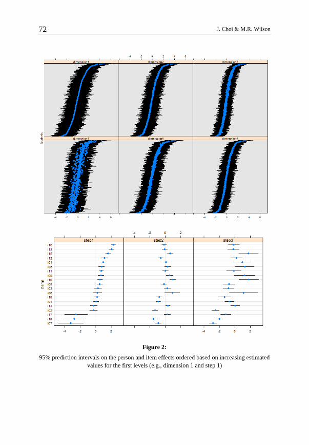
J. Choi & M.R. Wilson 72
Figure 2:
95% prediction intervals on the person and item effects ordered based on increasing estimated
values for the first levels (e.g., dimension 1 and step 1)
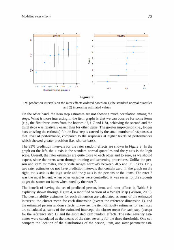
Modeling rater effects 73
Figure 3:
95% prediction intervals on the rater effects ordered based on 1) the standard normal quantiles
and 2) increasing estimated values
On the other hand, the item step estimates are not showing much correlation among the
steps. What is more interesting in the item graphs is that we can observe for some items
(e.g., the first three items from the bottom: i7, i17 and i18), achieving the second and the
third steps was relatively easier than for other items. The greater imprecision (i.e., longer
bars crossing the estimate) for the first step is caused by the small number of responses at
that level of performance, compared to the responses at higher levels of performances
which showed greater precision (i.e., shorter bars).
The 95% prediction intervals for the rater random effects are shown in Figure 3. In the
graph on the left, the x axis is the standard normal quantiles and the y axis is the logit
scale. Overall, the rater estimates are quite close to each other and to zero, as we should
expect, since the raters went through training and screening procedures. Unlike the per-
son and item estimates, the y scale ranges narrowly between -0.5 and 0.5 logits. Only
two rater estimates do not have prediction intervals that contain zero. In the graph on the
right, the x axis is the logit scale and the y axis is the persons or the items. The rater 7
was the most lenient: when other variables were controlled, it was easier for the students
to get the scores on items when rated by the rater 7.
The benefit of having the set of predicted person, item, and rater effects in Table 3 is
explicitly shown through Figure 4, a modified version of a Wright Map (Wilson, 2005).
The person ability estimates for each dimension are calculated as sums of the estimated
intercept, the cluster mean for each dimension (except the reference dimension 1), and
the estimated person random effects. Likewise, the item difficulty estimates for each step
are calculated as sums of the estimated intercept, the cluster mean for each step (except
for the reference step 1), and the estimated item random effects. The rater severity esti-
mates were calculated as the means of the rater severity for the three thresholds. One can
compare the location of the distributions of the person, item, and rater parameter esti-

J. Choi & M.R. Wilson 74
mates on the same logit scale, which gives insight into how easy it was for the students
to get the target score on the items by the raters.
The person ability scores are displayed as density curves on the logit scale. Dimensions 3
and 4 have relatively small variances and the shape of dimension 4 density is slightly off
from the symmetric normal distribution. The ability distributions of the six dimensions
shared similar locations and dispersions, again validating the finding that the multidi-
mensional model does not fit the data better than the unidimensional one. The result
corresponds with the lower latent correlation for dimension 4 with other dimensions as
well as the fuzzy dots in the 95% prediction interval graph. Most likely, the reason why
dimension 4 behaves as an oddity is the very low number of items (2) that measures it.
Next, the three groups of points represent item difficulties. The location of the points can
be interpreted as where the students on average have a 50% probability to get a particular
score as compared to a score below that. Since the data had four possible scores
(0,1,2,3), three steps or thresholds exist between the four scores. As the Wright Map
shows, most of the students had more than 50% chance to achieve the first thresholds of
all items, except for the items 13 to 16. In other words, for most of the students, getting
the score 1 versus 0 was relatively easy. The second thresholds of the items were reason-
ably located near the means of the person distributions, meaning that on average students
were able to get the score 2 on most items with about a 50% probability of success. Get-
ting the highest score was generally difficult for the students, particularly for the items 1,
5, 6, 9, and 15.
Last, the raters were generally non-separable from each other except for the rater 6 and 7
who were on average more lenient than others in giving scores (compared to the score
below) for the items to the students. The small variance component, the small resulting
generalizability coefficient, and non-separable individual rater effects that we found in
this analysis suggest that the rater training sessions were highly effective. The eight
raters were indeed graduate research assistants who were involved in every stage of the
research process — thus for this group of raters it makes sense that they showed con-
sistent ratings.
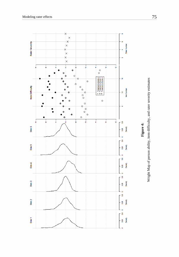
Modeling rater effects 75
Fig
ure
4:
Wri
ght
Map
of
per
son a
bil
ity
, it
em d
iffi
cult
y,
and
rat
er s
ever
ity
est
imat
es

J. Choi & M.R. Wilson 76
Discussion
In this study, we have suggested an approach for combining GT and IRT. We recognize
that IRT models can be written in terms of a latent continuous response and that a classic
IRT model can be modeled directly using a simple GT design with items as a fixed facet.
The resulting logistic mixed models extend a classic IRT model by treating items as a
random facet and/or considering other facets such as raters. The advantage of the pro-
posed approach is that it allows a straightforward maximum likelihood estimation of
individual random effects as well as the variance components needed for the generaliza-
bility coefficients.
In addition, application of the proposed approach was illustrated using a moderately
large-scale education data set. The results demonstrated another advantage of the pro-
posed approach: its flexibility with respect to incorporating extra complications in meas-
urement situations (e.g., multidimensionality, polytomous responses) and explanatory
variables (e.g., rater facet). The variance components and the generalizability coeffi-
cients were presented. Also, predicted individual random effects were presented by tak-
ing advantage of the usefulness of a modified Wright Map.
The results motivate further research on the following. In suggesting an approach to
combine GT and IRT, the robustness of the generalizability coefficient estimates may not
necessarily become a concern. However, the effects of (a) the discrete nature of data
(e.g., more than two categories), (b) the violation of normality assumptions, and (c) more
complex designs (e.g., person by item by rater design, multidimensionality), on the esti-
mation accuracy of the variance components and the generalizability coefficients, should
be examined and reported.
The proposed approach can be generalized to other measurement situations, both simpler
and more complex ones. A simpler example is a balanced design with no missing data, or
a design where the facets are nested. A more complex example is an unbalanced design
with more than three crossed facets. For example, in addition to person, item, and rater
facets, one could include an occasion facet that involves repeated measurement. Such
attempts may offer an even closer connection between existing GT designs and IRT
models. Currently, research is underway to extend the proposed approach to such alter-
native designs. It is in our hopes that the results from these studies will provide a more
comprehensive basis to understand and evaluate methodological advantages and disad-
vantages of the existing and proposed approaches.
In the meantime, whether the proposed method is extendable to different designs, such as
nested designs or designs with more than three facets, partly depends on the estimation
methods chosen. Until recently, estimation of crossed random effects models has been
limited to a relatively small number of random effects, or facets, and their levels. Even
though the flexibility of the proposed approach allows a straightforward extension of the
models to those situations, questions remain regarding how to estimate the variance
components in the models with an increased number of crossed random facets. Moreo-
ver, incorporating other item parameters such as discrimination differences or guessing
in IRT models may add more challenges in estimation and interpretation. It will be inter-

Modeling rater effects 77
esting to investigate what advanced and/or alternative estimation methods might be
needed in extending the approaches to combine GT and IRT.
Lastly, an interesting topic for further studies exists around understanding the interaction
effect between raters and persons (i.e., ratees). For example, a rater’s rating of a person’s
response can differ systematically based on the characteristics of the response that the
person gave. An interaction can also exist between the persons’ group membership and
the raters. For example, some raters might rate female students’ responses differently
than male students’ responses. Or raters might differ their ratings systematically between
groups of students, not knowing which group each student belongs to. Jin & Wang
(2017) recently discussed a mixture facets model to account for differential rater func-
tioning — the interaction between the ratees’ unknown group membership and raters. In
the proposed approach the interaction between individual raters and individual persons
can be either included or not included, although it was not the focus of this study to fully
explore this topic. As interactions between these facets can occur in real testing situa-
tions, it will be worthwhile to further explore how best we can model this effect.
Conclusion
The integrated modeling approach provides advantages by combining GT and IRT anal-
yses. The logistic mixed model allows for a straightforward and effective maximum
likelihood estimation of individual random effects for IRT analysis as well as the vari-
ance components needed for GT analysis. Through the Laplacian approximation imple-
mented in the lmer() function in R, it estimates more than one cross-classified random
effect efficiently with regard to the calculation time; and it estimates the variance com-
ponents of incomplete data from the unbalanced mixed design relatively easily, without
producing negative variance estimates. The findings from the sample data analysis
showed that the proposed approach can be extended to more complicated test conditions
(e.g., multidimensionality, polytomous responses, multiple raters) and produces individ-
ual estimates for persons, items, and rater random effects as well as the generalizability
coefficients for person, item, and rater facets.
References
Agresti, A., & Kateri, M. (2011). Categorical data analysis. In The International Encyclopedia
of Statistical Science (pp. 206-208). Berlin: Springer.
Andrich, D. (1978). A rating formulation for ordered response categories. Psychometrika,
43(4), 561-573.
Bates, D. M. (2010). lme4: Mixed-effects modeling with R. URL http://lme4.r-forge.r-
project.org/book.
Bates, D., Mächler, M., Bolker, B., & Walker, S. (2014). Fitting linear mixed-effects models
using lme4. arXiv preprint arXiv:1406.5823.

J. Choi & M.R. Wilson 78
Brennan, R. L. (2001). Generalizability theory. New York, NY: Springer.
Breslow, N. E., & Clayton, D. G. (1993). Approximate inference in generalized linear mixed
models. Journal of the American Statistical Association, 88, 9–25.
Briggs, D. C., & Wilson, M. R. (2007). Generalizability in item response modeling. Journal
of Educational Measurement, 44(2), 131–155.
Chien, Y. M. (2008). An investigation of testlet-based item response models with a ran-
dom facets design in generalizability theory. Doctoral dissertation. The University of Io-
wa.
Cho, S. J., & Rabe-Hesketh, S. (2011). Alternating imputation posterior estimation of models
with crossed random effects. Computational Statistics & Data Analysis, 55(1), 12-25.
Choi, J. (2013). Advances in combining Generalizability Theory and Item Response Theory.
Doctoral dissertation. University of California, Berkeley: Berkeley, CA.
Choi, J., Briggs, D. C., & Wilson, M. R. (2009, April). Multidimensional extension of the
generalizability in item response modeling (GIRM). Paper presented at the 2009 National
Council on Measurement in Education Annual Meeting, San Diego, CA.
Choi, J., Lee, Y.-S. & Draney, K. (2009). Principle-based and process-based multidimen-
sionality and rater effects in validation of the carbon cycle learning progression. Paper
presented at the American Educational Research Association Annual Meeting, San Diego,
CA.
Cronbach, L. J., Gleser, G. C., Nanda, H., & Rajaratnam, N. (1972). The dependability of
behavioral measurements: Theory of generalizability for scores and profiles. New York,
NY: Wiley.
De Boeck, P., Bakker, M., Zwitser, R., Nivard, M., Hofman, A., Tuerlinckx, F., & Partchev, I.
(2011). The estimation of item response models with the lmer function from the lme4
package in R. Journal of Statistical Software, 39, 1–28.
Fahrmeir, L., & Tutz, G. (2001). Multivariate statistical modeling based on generalized linear
models (2nd ed.). New York, NY: Springer.
Gałecki, A., & Burzykowski, T. (2013). Linear mixed-effects models using R: A step-by-step
approach. New York, NY: Springer.
Gelman, A. (2005). Analysis of variance — why it is more important than ever. Annals of
Statistics, 33(1), 1-53.
Gelman, A., Carlin, J. B., Stern, H. S., & Rubin, D. B. (2003). Bayesian data analysis. Boca
Raton, FL: Chapman & Hall/CRC.
Iramaneerat, C., Yudkowsky, R., Myford, C., & Downing, S. (2008). Quality control of an
OSCE using generalizability theory and many-faceted Rasch measurement. Advances in
Health Sciences Education, 13(4), 479–493.
Jin, K. Y., & Wang, W. C. (2017). Assessment of differential rater functioning in latent clas-
ses with new mixture facets models. Multivariate Behavioral Research, 52(3), 391–402.
Joe, H. (2008). Accuracy of Laplace approximation for discrete response mixed models.
Computational Statistics and Data Analysis, 52, 5066–5074.

Modeling rater effects 79
Khuri, A. I. (2000). Designs for variance components estimation: Past and present. Interna-
tional Statistical Review, 68(3), 311-322.
Khuri, A. I., & Sahai, H. (1985). Variance components analysis: A selective literature survey.
International Statistical Review/Revue Internationale de Statistique, 279-300.
Kolen, M., & Harris, D. (1987, April). A multivariate test theory model based on item re-
sponse theory and generalizability theory. Paper presented at the annual meeting of the
American Educational Research Association, Washington, DC.
Linacre, J. M. (1993, April). Generalizability theory and many-facet Rasch measurement.
Paper presented at the annual meeting of the American Educational Research Association,
Atlanta, GA.
Lord, F. M. (1980). Applications of item response theory to practical testing problems. Hills-
dale, NJ: Erlbaum.
Lynch, B. K., & McNamara, T. F. (1998). Using G-theory and many-facet Rasch measure-
ment in the development of performance assessments of the ESL speaking skills of immi-
grants. Language Testing, 15(2), 158-180.
MacMillan, P. D. (2000). Classical, generalizability, and multifaceted Rasch detection of
interrater variability in large, sparse data sets. Journal of Experimental Education, 68,
167–190.
Masters, G. N. (1982). A Rasch model for partial credit scoring. Psychometrika, 47(2), 149-
174.
Patz, R. J., Junker, B. W., Johnson, M. S., & Mariano, L. T. (2002). The hierarchical rater
model for rated test items and its application to large-scale educational assessment data.
Journal of Educational and Behavioral Statistics, 27(4), 341–384.
Pearson, K. (1901). Principal components analysis. The London, Edinburgh and Dublin Phil-
osophical Magazine and Journal, 6(2), 566.
Pinheiro, J. C., & Bates, D. M. (1995). Approximations to the log-likelihood function in the
nonlinear mixed-effects model. Journal of Computational and Graphical Statistics, 4(1),
12-35.
R Core Team (2017). R: A language and environment for statistical computing. R Foundation
for Statistical Computing, Vienna, Austria. URL https://www.R-project.org/.
R Development Core Team (2011). R: A language and environment for statistical computing.
R Foundation for Statistical Computing, Vienna, Austria. ISBN 3-900051-07-0, URL
http://www.r-project.org/.
Rabe-Hesketh, S., Skrondal, A., & Pickles, A. (2004). Generalized multilevel structural equa-
tion modeling. Psychometrika, 69(2), 167-190.
Rasch, G. (1960). Probabilistic models for some intelligence and attainment tests. Copenha-
gen, Denmark: Denmarks Pedagogiske Institut.
Robinson, G. K. (1991). That BLUP is a good thing: The estimation of random effects. Statis-
tical Science, 15-32.
Samejima, F. (1997). Graded response model. In W. J. van der Linden & R. K. Hambleton
(Eds.), Handbook of modern item response theory (pp. 85-100). New York: Springer.

J. Choi & M.R. Wilson 80
Skrondal, A., & Rabe-Hesketh, S. (2004). Generalized latent variable modeling: Multilevel,
longitudinal, and structural equation models. Boca Raton, FL: Chapman & Hall/CRC.
Smith, E. V., & Kulikowich, J. M. (2004). An application of generalizability theory and
many-facet Rasch measurement using a complex problem solving skills assessment. Edu-
cational and Psychological Measurement, 64, 617–639.
Sudweeks, R. R., Reeve, S., & Bradshaw, W. S. (2005). A comparison of generalizability
theory and many-facets Rasch measurement in an analysis of college sophomore writing.
Assessing Writing, 9(3), 239–261.
Tutz, G. (1990). Sequential item response models with an ordered response. British Journal of
Mathematical and Statistical Psychology, 43, 39–55.
Wilson, M. (2005). Constructing measures: An item response modeling approach. Mahwah,
NJ: Erlbaum.
Wright, B. D., & Stone, M. A. (1979). Best test design. Chicago, IL: MESA Press,
Wu, M. L., Adams, R. J., Wilson, M. R., & Haldane, S. A. (2007). ACER ConQuest version
2.0: Generalised item response modelling software [Computer software and manual].
Camberwell, Australia: ACER Press.
Zheng, X., & Rabe-Hesketh, S. (2007). Estimating parameters of dichotomous and ordinal
item response models with gllamm. Stata Journal, 7(3), 313-333.
Appendix
We provide generic examples of lmer() syntax for logistic mixed models with crossed
random effects. In the syntax, we assume that the name of dataset is ‘data’. Syntax for
simpler models have been also provided for comparisons. We recommend Gałecki &
Burzykowski (2013) for details in specifying linear mixed effects models using R. Please
contact authors for further assistance with model specification.
(a) Main effects for persons, items, and raters
R> lmer(y ~ personid + itemid + raterid, data=data,
family=binomial)
(b) Main effects with random intercepts for persons, items, and raters
R> lmer(y ~ (1|personid) + (1|itemid) + (1|raterid),
data=data, family=binomial)
(c) Crossed random effects with random intercepts for persons, items, raters and their
interactions
R> lmer(y ~ (1|personid) + (1|itemid) + (1|raterid) +
personid:itemid + personid:raterid + per
sonid:itemid:raterid , data=data, family=binomial)
Psychological Test and Assessment Modeling, Volume 60, 2018 (1), 81-100
Comparison of human rater and automated scoring of test takers’ speaking ability and classification using Item Response Theory Zhen Wang1 & Yu Sun2
Abstract Automated scoring has been developed and has the potential to provide solutions to some of the obvious shortcomings in human scoring. In this study, we investigated whether SpeechRaterSM and a series of combined SpeechRaterSM and human scores were comparable to human scores for an English language assessment speaking test. We found that there were some systematic patterns in the five tested scenarios based on item response theory.
Keywords: SpeechRaterSM, human scoring, item response theory, ability estimation and classification
1Correspondence concerning this article should be addressed to: Zhen (Jane) Wang, Educational Testing
Service, Senior Psychometrician, Psychometrics, Statistics and Data Sciences (PSDS), Rosedale-Anrig, Princeton, NJ, U.S.A; email: [email protected].
2Senior Psychometric Analyst, Psychometrics, Statistics and Data Sciences (PSDS), Rosedale-Anrig, Princeton, NJ,

Z. Wang & Y. Sun 82
Language testing organizations in the United States routinely deal with large test taker samples, especially for certain Asian, European, and mid–eastern countries. For example, it is not unusual to have more than a million test takers worldwide taking a certain test in a given year, with each test taker responding to six items producing a total of more than six million responses. While having large samples is certainly not exclusive to language testing, constructed response item scoring, including essay scoring and spoken response scoring, is definitely an added complication for scoring. Human scoring must be closely monitored within each administration and across admin-istrations to ensure the quality and consistency of the human ratings. The effects of differ-ences between human raters may substantially increase the bias in test takers’ final scores without careful monitoring (Wang & Yao, 2013). This makes human scoring very labor intensive, time consuming and expensive (Zhang, 2013). The importance of these language tests for relatively high stake decisions places a lot of pressure on the entire system to ensure accurate scoring and consistent ratings on demand. Automated scoring has been developed and has the potential to provide solutions to some of the obvious shortcomings in human scoring (e.g., rater inconsistency; rater drift; ineffi-ciency). Bennett and Bejar (1998) indicated that automated scoring procedures allow for the scoring rules to be applied consistently. Automated scoring has some advantages in-cluding “fast scoring, constant availability of scoring, lower per unit costs, greater score consistency, reduced coordination efforts for human raters, and potential for a degree of performance specific feedback” (Ramineni, Trapani, Williamson, Davey, & Bridgeman, 2012). Recently, more and more operational scoring programs have started using auto-mated scoring to augment human scorers. In the literature, we found some studies on the comparison of human and automated scoring conducted in recent years (Attali, Bridgeman & Trapani, 2010; Attali & Burstein, 2006; Chodorow & Burstein, 2004; Laundauer, Laham, & Foltz, 2003; Nichols, 2005; Ramineni et al., 2012; Streeter, Bernstein, Foltz, & Deland, 2011; Wang & von Davier, 2014; Wang, Zechner & Sun, 2016; Williamson, Xi, & Breyer, 2012). Wang et al. (2016) conducted a comprehensive analysis of SpeechRaterSM and human scoring at item, rater and form levels based on the speaking data from 10 administrations. For automated scoring, there is no need to examine changes in rater severity. Automated scoring is not prone to these types of changes. However, if an engine update occurs, the scores need to be investigated for comparability against human rater scores. As Attali (2013) pointed out, the relation of automated scores to human scores provides important information about the validity of automated scores. In terms of operational scoring, several researchers have called for the need to study how to combine human and machine scores (Attali, 2013; Zhang, Breyer, & Lorenz, 2013), which is lacking in the current research literature. Due to the shortcomings of human rater and automated scoring, the argument of combining the two is appealing. The shift to the combination of the two allows us to move beyond using human scoring as the default “gold standard” and become less concerned about the construct underrepresentation of the auto-mated scoring. The primary purpose of the present research is to investigate whether human raters and SpeechRaterSM scores and different combinations of the two are comparable for test takers’ final scoring, ability estimation, and classification.
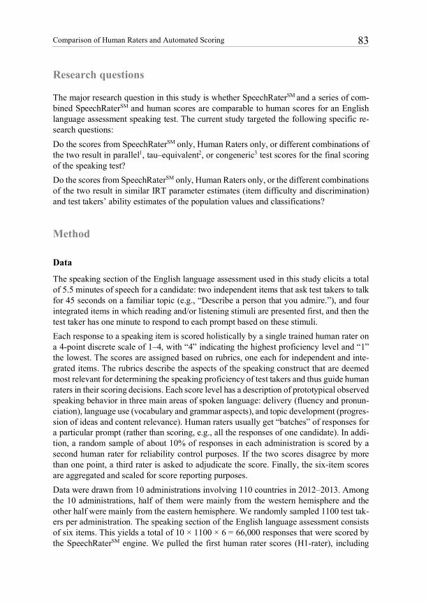
Comparison of Human Raters and Automated Scoring 83
Research questions
The major research question in this study is whether SpeechRaterSM and a series of com-bined SpeechRaterSM and human scores are comparable to human scores for an English language assessment speaking test. The current study targeted the following specific re-search questions: Do the scores from SpeechRaterSM only, Human Raters only, or different combinations of the two result in parallel1, tau–equivalent2, or congeneric3 test scores for the final scoring of the speaking test? Do the scores from SpeechRaterSM only, Human Raters only, or the different combinations of the two result in similar IRT parameter estimates (item difficulty and discrimination) and test takers’ ability estimates of the population values and classifications?
Method
Data
The speaking section of the English language assessment used in this study elicits a total of 5.5 minutes of speech for a candidate: two independent items that ask test takers to talk for 45 seconds on a familiar topic (e.g., “Describe a person that you admire.”), and four integrated items in which reading and/or listening stimuli are presented first, and then the test taker has one minute to respond to each prompt based on these stimuli. Each response to a speaking item is scored holistically by a single trained human rater on a 4-point discrete scale of 1–4, with “4” indicating the highest proficiency level and “1” the lowest. The scores are assigned based on rubrics, one each for independent and inte-grated items. The rubrics describe the aspects of the speaking construct that are deemed most relevant for determining the speaking proficiency of test takers and thus guide human raters in their scoring decisions. Each score level has a description of prototypical observed speaking behavior in three main areas of spoken language: delivery (fluency and pronun-ciation), language use (vocabulary and grammar aspects), and topic development (progres-sion of ideas and content relevance). Human raters usually get “batches” of responses for a particular prompt (rather than scoring, e.g., all the responses of one candidate). In addi-tion, a random sample of about 10% of responses in each administration is scored by a second human rater for reliability control purposes. If the two scores disagree by more than one point, a third rater is asked to adjudicate the score. Finally, the six-item scores are aggregated and scaled for score reporting purposes. Data were drawn from 10 administrations involving 110 countries in 2012–2013. Among the 10 administrations, half of them were mainly from the western hemisphere and the other half were mainly from the eastern hemisphere. We randomly sampled 1100 test tak-ers per administration. The speaking section of the English language assessment consists of six items. This yields a total of 10 × 1100 × 6 = 66,000 responses that were scored by the SpeechRaterSM engine. We pulled the first human rater scores (H1-rater), including

Z. Wang & Y. Sun 84
second human rater scores (H2-rater, if available), from a data repository (note that “H1” and “H2” are logical labels for human raters; in actuality, each of “H1” scores and “H2” scores comprise scores from a large number of human raters.) As stated above, H2-rater scores were only available for 10% of the data, which is a random sample from the admin-istrations selected for reliability purposes. During the operational cycle, all human raters (both H1-rater and H2-rater) participated in a standardized training process before they were allowed to rate the speaking items. In this study, we focused on the comparison of the item scores between the H1-rater and SpeechRaterSM. The H2-rater was from the same rater pool as the H1-rater, so there should not be any systematic differences between the results from the H1-rater and the H2-rater. We also made comparisons between the scores assigned by the H1-rater and the H2-rater for the 10% reliability sample. In addition to the main data set used for this study (66,000 spoken responses), we used 10,000 spoken responses to items in other forms of the same assessment to estimate the parameters of the linear regression model used by SpeechRaterSM (discussed in next sec-tion). A separate data set of 52,200 responses from the same assessment was used for training the parameters of the ASR system.
SpeechRaterSM
SpeechRaterSM is an automated scoring engine developed at ETS that has been used in the TOEFL Practice Online program since 2006. It consists of an automatic speech recognizer (ASR system), feature computation modules, filtering model, a multiple regression scoring model to predict scores produced by human scorers for each spoken response (Zechner, Higgins, Xi, & Williamson, 2009). The filtering model, used to filter out non-scorable responses, is an important component of SpeechRaterSM (Higgins, Xi, Zechner, & Wil-liamson, 2011). In recent years, the coverage of the speaking construct has been substan-tially extended from its original focus on fluency, pronunciation, and prosody by adding features related to vocabulary, grammar, and content, among others (Chen & Zechner, 2011; Xie, Evanini, & Zechner, 2012; Yoon & Bhat, 2012; Yoon, Bhat, & Zechner, 2012).
Data analyses
Classical analyses
Score comparisons using classical analysis were made based on different scoring scenar-ios. Analyses were conducted to answer the question of whether scoring based on the SpeechRaterSM only, human raters only, or combinations of the two would result in paral-lel, tau-equivalent, or congeneric test scores for the final scoring of the speaking test. Different scoring scenarios tested include the following five scores:
S1. Human rater (H1-rater) only;

Comparison of Human Raters and Automated Scoring 85
S2. SpeechRaterSM only; S3. Total of SpeechRaterSM and human rater; S4. Lower weighting (1/3) on human and higher weighting (2/3) on
SpeechRaterSM; S5. Higher weighting (2/3) on human and lower weighting (1/3) on SpeechRaterSM.
The above scenarios can also be expressed as different weights in the weighted sum of the two ratings (human rater and SpeechRaterSM, respectively):
S1. (1, 0); S2. (0, 1); S3. (1/2, 1/2); S4. (1/3, 2/3); S5. (2/3, 1/3).
The one-factor measurement model was initially tested within the linear structural equa-tion framework of Jöreskog and Sörbom (1984). A single-factor measurement model was fit to the data, in which all the five speaking scores were set to load on the same common latent variable representing the English speaking ability construct. The five different scoring scenarios (S1 – S5 above) for the final speaking scores, which are the aggregated score across all six speaking items, were considered as five measures (S1 – S5), each measure was based on the same speaking items in the test. Reliability was calculated for each of the scoring scenarios. Correlations were also calculated among the five measures based on the different scoring scenarios. Parallel measures are the most re-strictive model, assuming equal true score variances and equal error variances. Tau-equiv-alent measures have equal true score variances, but possibly different error variances whereas congeneric models allow true score variances as well as error variances to differ. Covariance matrices were analyzed and weighted least squares estimates of the parameters were obtained. If the fit of the model to the data becomes worse as the model is made more restrictive, then the constraints are not plausible for the data (Maruyama, 1998). Three fit indices were used to evaluate the model-data fit, root mean squared error approx-imation (RMSEA), comparative fit index (CFI), and the normed fit index (NFI). Some empirical guidelines were followed when evaluating these fit indices: a model with an RMSEA value below .08, a CFI value above .90, a NFI value above .90, were considered to be an acceptable fit; a model with an RMSEA value below .05 and a CFI (and NFI) value above .95 were considered a good fit (Browne & Cudeck, 1993; Hooper, Coughlan, & Mullen, 2008; & Hu & Bentler, 1999).

Z. Wang & Y. Sun 86
IRT analyses
Generalized partial credit model. PARSCALE (Muraki & Bock, 1997) was used to analyze the speaking tests based on the Generalized Partial Credit Model (GPCM, Muraki, 1992). The normal distribution was used as the prior distribution of ability. The method employed in the calibration phase of PARSCALE is that of random-effects estimation through marginal maximum likelihood. The random-effects solution employs the EM method (estimation and maximization) of solving the marginal likelihood equations. We set the number of EM cycles to be 50, and the number of quadrature points as 41 in the EM and Newton estimation. The scale param-eter was set at 1.7 in the PARSCALE run. Each speaking item was analyzed with IRT models with the following scoring designs: a) with human rater only; b) with SpeechRaterSM only; c) with the sum of human and SpeechRaterSM; d) with different weighting: 1/3 of human and 2/3 of SpeechRaterSM; and e) with different weighting: 2/3 of human and 1/3 of SpeechRaterSM. A key goal of this study was to compare test takers’ ability estimates, and IRT parameters from different scoring designs. To compare test takers’ ability estimates and IRT parameters, we used squared bias and the mean squared error. Root mean squared error (RMSE), absolute mean bias (ABSBIAS), and bias were com-puted for all parameters and were used to examine the IRT parameter estimate differences, such as ability, difficulty, and discrimination. For example, let fref be the ability parameter based on the scoring with human rater 1 only (reference) and let be the SpeechRaterSM
only or the combination of the two (see S1 to S5 above), then
𝑅𝑀𝑆𝐸 = &1𝑛)
(𝑓, − 𝑓./0)23
,45
(1)
where is the number of test takers. Here f represents ability parameter estimates.
The bias and absolute mean bias are defined as the following:
𝐵𝐼𝐴𝑆 = &1𝑛)
(𝑓, − 𝑓./0)3
,45
(2)
𝐴𝐵𝑆𝐵𝐼𝐴𝑆 =1𝑛)9(𝑓, − 𝑓./0)9
3
,45
(3)
jf
n

Comparison of Human Raters and Automated Scoring 87
Bias and absolute mean bias were used to assess the parameter estimate differences. The squared differences and squared bias were also calculated and plotted to show results of parameter estimate differences and comparison among different scoring scenarios.
Results
Research question 1
Do the scores obtained from SpeechRaterSM only, Human Raters only, or the different combinations of the two result in parallel, tau-equivalent, or congeneric test scores for the final scoring of the speaking test?
Correlations.
Correlations were calculated (see Table 1) among the five scores (S1 – S5) based on dif-ferent scoring scenarios (H1-rater only; SpeechRaterSM only; sum of SpeechRaterSM and H1-rater; lower weighting on human and higher weighting on SpeechRaterSM; higher weighting on human and lower weighting on SpeechRaterSM). The lowest correlation (.759) was found between the scores from H1-rater only and SpeechRaterSM only, and the other correlations range from .866 to .994.
Table 1: Correlations among Five Scoring Scenarios (S1 – S5)
H1 only
SR only
H1+SR 1/3H1+2/3SR 2/3H1+1/3SR Mean SD
S1: H1 only 1 16.11 3.40 S2: SR only 0.759 1 16.01 2.52 S3:1/2H1+1/2SR 0.956 0.917 1 32.12 5.56 S4:1/3H1+2/3SR 0.911 0.960 0.992 1 16.04 2.64 S5:2/3H1+1/3SR 0.983 0.866 0.994 0.971 1 16.07 2.96
Reliability
Reliability was calculated for the five different scoring scenarios for each form. The reli-ability for H1 was the lowest, ranging from .85–.89 across all the speaking items, the reli-ability for SR only was the highest, ranging from .94–.96; the other combinations had reliabilities above .89 for all the speaking items, see Table 2 below.
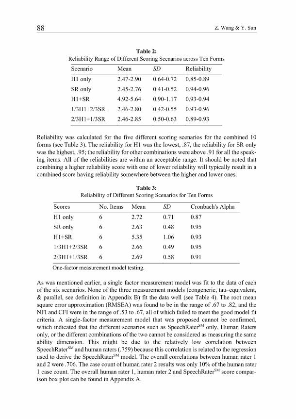
Z. Wang & Y. Sun 88
Table 2: Reliability Range of Different Scoring Scenarios across Ten Forms
Scenario Mean SD Reliability
H1 only 2.47-2.90 0.64-0.72 0.85-0.89 SR only 2.45-2.76 0.41-0.52 0.94-0.96 H1+SR 4.92-5.64 0.90-1.17 0.93-0.94 1/3H1+2/3SR 2.46-2.80 0.42-0.55 0.93-0.96 2/3H1+1/3SR 2.46-2.85 0.50-0.63 0.89-0.93
Reliability was calculated for the five different scoring scenarios for the combined 10 forms (see Table 3). The reliability for H1 was the lowest, .87, the reliability for SR only was the highest, .95; the reliability for other combinations were above .91 for all the speak-ing items. All of the reliabilities are within an acceptable range. It should be noted that combining a higher reliability score with one of lower reliability will typically result in a combined score having reliability somewhere between the higher and lower ones.
Table 3: Reliability of Different Scoring Scenarios for Ten Forms
Scores No. Items Mean SD Cronbach's Alpha
H1 only 6 2.72 0.71 0.87 SR only 6 2.63 0.48 0.95 H1+SR 6 5.35 1.06 0.93 1/3H1+2/3SR 6 2.66 0.49 0.95 2/3H1+1/3SR 6 2.69 0.58 0.91
One-factor measurement model testing.
As was mentioned earlier, a single factor measurement model was fit to the data of each of the six scenarios. None of the three measurement models (congeneric, tau–equivalent, & parallel, see definition in Appendix B) fit the data well (see Table 4). The root mean square error approximation (RMSEA) was found to be in the range of .67 to .82, and the NFI and CFI were in the range of .53 to .67, all of which failed to meet the good model fit criteria. A single-factor measurement model that was proposed cannot be confirmed, which indicated that the different scenarios such as SpeechRaterSM only, Human Raters only, or the different combinations of the two cannot be considered as measuring the same ability dimension. This might be due to the relatively low correlation between SpeechRaterSM and human raters (.759) because this correlation is related to the regression used to derive the SpeechRaterSM model. The overall correlations between human rater 1 and 2 were .706. The case count of human rater 2 results was only 10% of the human rater 1 case count. The overall human rater 1, human rater 2 and SpeechRaterSM score compar-ison box plot can be found in Appendix A.
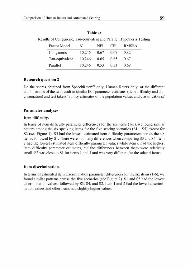
Comparison of Human Raters and Automated Scoring 89
Table 4: Results of Congeneric, Tau-equivalent and Parallel Hypothesis Testing
Factor Model N NFI CFI RMSEA
Congeneric 10,246 0.67 0.67 0.82 Tau-equivalent 10,246 0.65 0.65 0.67 Parallel 10,246 0.53 0.53 0.68
Research question 2
Do the scores obtained from SpeechRaterSM only, Human Raters only, or the different combinations of the two result in similar IRT parameter estimates (item difficulty and dis-crimination) and test takers’ ability estimates of the population values and classifications?
Parameter analyses
Item difficulty. In terms of item difficulty parameter differences for the six items (1-6), we found similar pattern among the six speaking items for the five scoring scenarios (S1 – S5) except for S2 (see Figure 1). S5 had the lowest estimated item difficulty parameters across the six items, followed by S1. There were not many differences when comparing S3 and S4. Item 2 had the lowest estimated item difficulty parameter values while item 6 had the highest item difficulty parameter estimates, but the differences between them were relatively small. S2 was close to S1 for items 1 and 4 and was very different for the other 4 items.
Item discrimination.
In terms of estimated item discrimination parameter differences for the six items (1-6), we found similar patterns across the five scenarios (see Figure 2). S1 and S5 had the lowest discrimination values, followed by S3, S4, and S2. Item 1 and 2 had the lowest discrimi-nation values and other items had slightly higher values.

Z. Wang & Y. Sun 90
Figure 1: Comparison of estimated difficulty parameters across five different scoring scenarios for
the six speaking items.
Figure 2:
Comparison of estimated discrimination parameters across five different scoring scenar-ios for the six speaking items.

Comparison of Human Raters and Automated Scoring 91
Bias analyses
Ability estimates In terms of test takers’ estimated ability differences (see Figure 3), S1 and S2 had the largest absolute bias, RMSE and bias when combining all six items, followed by S1 and S4, S1 and S3, and S1 and S5.
Figure 3:
Comparison of test takers’ estimated ability values: comparison of four scoring scenarios against human rater (S1):1=S2- S1; 2=S3-S1; 3=S4-S1; 4=S5-S1.
Location estimates.
In terms of test takers’ estimated location differences, S1 and S5 had the smallest absolute bias, RMSE and bias when combining all six items, followed by S1 and S2, S1 and S3, and S1 and S4 (Figure 4).
Figure 4:
Comparison of estimated location values: comparison of four scoring scenarios against human rater (S1):1=S2-S1; 2=S3-S1; 3=S4-S1; 4=S5-S1.
-0,4
-0,2
0
0,2
0,4
0,6
0,8
1
0 1 2 3 4 5ABSBIAS RMSE BIAS

Z. Wang & Y. Sun 92
Slope estimates.
In terms of test takers’ estimated slope differences, S1 and S2 had the largest absolute bias, RMSE and bias when combining all six items, followed by S1 and S4, S1 and S3, and S1 and S5 (Figure 5).
Figure 5:
Comparison of estimated slope values: comparison of four scoring scenarios against hu-man rater (S1): 1=S2-S1; 2=S3-S1; 3=S4-S1; 4=S5-S1.
Classification
We used 3 hypothetical estimated ability values (theta) cut scores (0.0, 0.6 and 1.6) to classify test takers. We found that S5 was close to S1 at all the cut scores, followed by S3, S4 and S2 (Table 5).
Table 5: Comparison of Test Takers’ Passing Rate across Different Scoring Scenarios
Theta=0.0 Diff vs S1
Theta=0.6 Diff vs S1
Theta=1.6 Diff vs S1
S1 46.06 – 32.19 – 5.43 – S2 53.56 7.5 40.61 8.42 4.64 -0.79 S3 47.79 1.73 33.79 1.60 4.40 -1.03 S4 52.84 6.78 37.94 5.75 3.87 -1.56 S5 45.76 -0.3 32.19 0.00 6.19 0.76

Comparison of Human Raters and Automated Scoring 93
Summary
In this paper, we summarized some findings regarding whether the scores obtained from SpeechRaterSM only, Human Raters only, or the different combinations of the two result in similar IRT parameters (item difficulty and discrimination) and test takers’ ability esti-mate and classifications. Below, we summarize the findings from our research and suggest recommendations for operational practice. For Research Question 1, we found that although the overall correlations between H1-rater scores and SpeechRaterSM scores were the lowest among all the different scoring designs, H1-rater had very high correlations with S5 and S3. The reliability for H1 was the lowest while the reliability for SR only was the highest (as would be expected because SR uses exactly the same criteria for scoring each time). A single-factor measurement model in the structural equation framework results indicated that all the different scoring scenarios such as SpeechRaterSM only, Human Raters only, or the different combinations of the two can-not be considered as measuring the same ability dimension. For Research Question 2, in terms of test takers’ estimated ability differences, S1 and S5 had the smallest absolute bias, RMSE and bias when combining all six items. For the clas-sification passing rate based on IRT ability estimates, the closest to H1-rater were S5 and S3. SpeechraterSM yielded different results when compared with H1-rater at 2 out of 3 cuts. We also investigated the raw score distribution of both H1-rater and SpeechraterSM scores and found that their distributions were different to some extent (see Figure 6 in the Ap-pendix). The fact that the score distributions differ would mean that different cut scores might result in different findings with respect to the classifications. The test information curves and standard error curves of the SpeechraterSM (S2) did not look similar to that of human rater (S1) (see Figures in Appendix C). Both test information curves and standard error curves indicated that S5 and S3 are closer to S1 than other scoring scenarios. Generally speaking, some of the main findings indicate that the SR-only approach is most different from the H1-only approach in comparison to the other approaches (for example, it has the lowest correlation of 0.759 and a completely different pattern of difficulty pa-rameter estimates across the six items, as shown in Figure 1). The explanation for these results would seem to be the fact that S3 - S6 all contain H1 in them (in combination with the SpeechRaterSM score), so it is a given that they will be more similar to S1 than S2.
Discussion
In this study, we used different approaches, such as classical and IRT modeling techniques to compare human rater and SpeechraterSM scores. We created different scoring scenarios based on arbitrary weights and investigated their differences. It seems that these ap-proaches are effective in detecting the differences between human and automated scoring; the research results can help practitioners make decisions in terms of how to combine hu-man and machine scores in the field. Identifying issues and differences between SpeechraterSM and human rater can help improve SpeechraterSM. However, the real data used for the human rater might not be perfect (Wang & Yao, 2013), which may have

Z. Wang & Y. Sun 94
prevented us from finding the real issue. Simulation studies are needed to compare SpeechraterSM and human rater in a controlled manner. In this study we used real data and investigated the differences between different scoring methods. We found that there are some systematic patterns in the combined scenarios based on both classical and IRT approaches, such as their raw score distributions, test information curves (see Appendix C), standard error curves (see Appendix C), and per-centage of passing rate. As pointed out above the percentage of passing rate results may well differ for different cut scores. The fact that S5 and S3 are closer to S1 than other scoring scenarios is within our expectation because they account for 1/2 and 2/3 of the human score. In this study, we compared the differences among different combinations of human and machine scores, and more such studies are needed (Attali, 2013; Zhang et al., 2013). We believe that the use of the statistical analyses (both classical and IRT) in this study is a useful way to advance the study of automated scoring in the evaluation of speech re-sponses. Our study can help our clients make decisions related to machine and human scoring. A future study is needed to provide guidelines about how to establish the set of weights that will generate optimal reliability to combine human rater and SpeechRaterSM scores. Reliability is just one criteria and there might be other criteria, such as validity that are also important to investigate. A simulation study should be conducted to test different scoring combination scenarios, and different cut scores, under different conditions.
Limitations
Since human raters’ scores are based on three areas (delivery, language use, and topic development) while SpeechRaterSM scores are based only on delivery and language use, differences between the two types of scores will probably always exist (and these differ-ences relate to validity issues). There are issues and questions that need to be investigated and answered before an automated speech scoring system such as SpeechRaterSM can be implemented for the operational scoring of English language assessment speaking items. We want to stress that the automated speech scoring engine SpeechRaterSM is still evolv-ing, and that additional features, covering a more extended subset of the Speaking con-struct, are currently under development and are planned for use in future scoring models. Moreover, we are also exploring alternative approaches to the standard linear regression scoring model currently used by SpeechRaterSM, which may lead to improvements in its scoring performance. The current SpeechraterSM distribution has high frequency at middle scores (see Figure 6 in the Appendix C), which may be due to the regression toward the mean effects from the linear regression scoring model.
Notes
1–3. See definitions in Appendix B.

Comparison of Human Raters and Automated Scoring 95
References
Attali, Y. (2013). Validity and reliability of automated essay scoring. In M. D. Shermis & J. Burstein (Eds.) Handbook of automated essay evaluation: Current applications and new directions (pp. 181-198). New York, NY: Routledge.
Attali, Y., Bridgeman, B., & Trapani, C. (2010). Performance of a generic approach in auto-mated scoring. Journal of Technology, Learning, and Assessment, 10, 1-16. Retrieved from http://www.jtla.org.
Attali, Y., & Burstein, J. (2006). Automated essay scoring with e–rater®v.2. Journal of Tech-nology, Learning, and Assessment, 4, 1-30. Retrieved from http://www.jtla.org.
Bennett, R. E., & Bejar, I. I. (1998). Validity and automated scoring: It's not only the scoring. Educational Measurement: Issues and Practice, 17, 9–17.
Browne, M. W., & Cudeck, R. (1993). Alternative ways of assessing model fit. In K. A. Bollen & J. S. Long (Eds.). Testing structural equation models (pp. 136–162). Beverly Hills, CA: Sage.
Chen, M., & Zechner, K. (2011). Computing and evaluating syntactic complexity features for automated scoring of spontaneous non–native speech. Proceedings of the 49th Annual Meeting of the Association for Computational Linguistics and the Human Language Tech-nologies Conference (ACL–HLT–2011) (pp.722-731). Portland, OR: Association for Com-putational Linguistics.
Chodorow, M., & Burstein, J. (2004). Beyond essay length: Evaluating e–rater®’s performance on essays (Research Report No. RR–04–04). Princeton, NJ: Educational Testing Service.
Higgins, D., Xi, X., Zechner, K., & Williamson, D. M. (2011). A three-stage approach to the automated scoring of spontaneous spoken responses. Computer Speech and Language, 25, 282-306.
Hooper, D., Coughlan, J., & Mullen, M. R. (2008). Structural equation modeling: Guidelines for determining model fit. Electronic Journal of Business Research Methods, 6, 3–60.
Hu, L., & Bentler, P. M. (1999). Cutoff criteria for fit indexes in covariance structure analysis: Conventional criterion versus new alternatives. Structural Equation Modeling, 6, 1–55.
Jöreskog, K., & Sörbom, D. (1984). LISREL IV: Analyses of linear structural relationships by maximum likelihood, instrumental variables, and least squares methods. Mooresville, IN: Scientific Software.
Laundauer, T. K., Laham, D. & Foltz, P. (2003). Automatic essay assessment. Assessment in Education, 10, 295–308.
Maruyama, G. (1998). Basics of structural equation modeling. Thousand Oaks CA: Sage. Nichols, P. (2005). Evidence for the interpretation and use of scores from an automated essay
scorer (White Paper). Iowa City, IA: Pearson.
Ramineni, C., Trapani, C., Williamson, D. M., Davey, T., & Bridgeman, B. (2012). Evaluation of e-rater® for the GRE issue and argument prompts (Research Report No. RR–12–06). Princeton, NJ: Educational Testing Service.

Z. Wang & Y. Sun 96
Streeter, L., Bernstein, J., Foltz, P., & Deland, D. (2011). Pearson’s automated scoring of writ-ing, speaking, and mathematics (White Paper). Iowa City, IA: Pearson.
Wang, Z., & von Davier, A. A. (2014). Monitoring of scoring using the e-rater automated scoring system and human raters on a writing test (Research Report No. RR–14–04). Princeton, NJ: Educational Testing Service.
Wang, Z., & Yao, L. (2013). Investigation of the effects of scoring designs and rater severity on students’ ability estimation using different rater models (ETS Research Report. No. RR–13–23). Princeton, NJ: Educational Testing Service.
Wang, Z., Zechner, K., & Sun, Y. (2016). Monitoring the performance of human and automated scores for spoken responses. Language Testing. Advance online publication. doi: 10.1177/0265532216679451
Williamson, D. M., Xi, X., & Breyer, F. J. (2012). A framework for evaluation and use of automated scoring. Educational Measurement: Issues and Practice, 31(1), 2–13.
Xie, S., Evanini, K., & Zechner, K. (2012). Exploring content features for automated speech scoring. Proceedings of North American Chapter of the Association for Computational Lin-guistics – Human Language Technologies (NAACL–HLT), Montreal, Canada: Association for Computational Linguistics.
Yoon, S. Y., & Bhat, S. (2012). Assessment of ESL learners' syntactic competence based on similarity measures. Paper presented at the Joint Conference on Empirical Methods in Nat-ural Language Processing and Computational Natural Language Learning (EMNLP-CoNLL) (pp. 600–608). Stroudsburg, PA: Association for Computational Linguistics.
Yoon, S.-Y., Bhat, S., & Zechner, K. (2012). Vocabulary profile as a measure of vocabulary sophistication. Paper presented at the 7th Workshop on Innovative Use of NLP for Building Educational Applications, North American Chapter of the Association for Computational Linguistics – Human Language Technologies (NAACL–HLT). Montreal, Canada: Associ-ation for Computational Linguistics.
Zechner, K., Higgins, D., Xi, X., & Williamson, D. M. (2009). Automatic scoring of non-native spontaneous speech in tests of spoken English. Special issue on Spoken Language Tech-nology for Education. Speech Communication, 51, 883–895.
Zhang, M. (2013). Contrasting automated and human scoring of essays. (R & D Connections, No. 21). Princeton, NJ: Educational Testing Service.
Zhang, M., Breyer, J., & Lorenz, F. (2013). Investigating the suitability of implementing e-rater in a large-scale English language testing program. (Research Report RR-13–36). Prince-ton, NJ: Educational Testing Service.

Comparison of Human Raters and Automated Scoring 97
Appendix A
Note. Human rater 2 is only 10% of the H1 data. Figure A1. Rater comparison between rater 1, rater 2 and SpeechRaterSM.
Appendix B
Parallel measures The measures (items) comprising a scale are parallel if the following two conditions hold:
1. for all i and j; τ = true scores; p = person;
2. for all i and j: e = error:
This implies that the amount of variation in the item score that is determined by the true score is the same for all items. It also implies that the expected value of each of the items will be the same.
Tau-equivalent measures
When measures are tau-equivalent, for all i and j, as in the case of parallel
measures, but we relax the assumption that for all i and j.
Rater comparison for overall
Rater 1 Rater 2 Speech Rater0
1
2
3
4
5
Sco
re
τ τip jp=
2 2ei ejs s=
τ τip jp=2 2ei ejs s=

Z. Wang & Y. Sun 98
Congeneric measures
Congeneric measures relax both the assumption that for all i and j, and that
for all i and j.
Appendix C
Test Information Curves and Standard Error Curves
Figure C1:
S1.
Figure C2:
S2
τ τip jp=2 2ei ejs s=
Test information curve: solid line Standard error curve: dotted lineThe total test information for a specific scale score is read from the left vertical axis.The standard error for a specific scale score is read from the right vertical axis.
-3 -2 -1 0 1 2 30
2
4
6
8
10
12
Scale Score
Info
rmat
ion
Test 1; Name: HR1
0
0.20
0.39
0.59
0.78
0.98
Standard Error
Test information curve: solid line Standard error curve: dotted lineThe total test information for a specific scale score is read from the left vertical axis.The standard error for a specific scale score is read from the right vertical axis.
-3 -2 -1 0 1 2 30
2
4
6
8
10
12
14
16
Scale Score
Info
rmat
ion
Test 1; Name: SP
0
0.18
0.35
0.53
0.71
0.88
Standard Error

Comparison of Human Raters and Automated Scoring 99
Figure C3:
S3.
Figure C4:
S4
Test information curve: solid line Standard error curve: dotted lineThe total test information for a specific scale score is read from the left vertical axis.The standard error for a specific scale score is read from the right vertical axis.
-3 -2 -1 0 1 2 30
2
4
6
8
10
12
Scale Score
Info
rma
tio
n
Test 1; Name: COMB1
0
0.16
0.32
0.48
0.64
0.80
Sta
nd
ard
Erro
r
Test information curve: solid line Standard error curve: dotted lineThe total test information for a specific scale score is read from the left vertical axis.The standard error for a specific scale score is read from the right vertical axis.
-3 -2 -1 0 1 2 30
2
4
6
8
10
12
14
16
Scale Score
Info
rmat
ion
Test 1; Name: COMB3
0
0.14
0.27
0.41
0.55
0.69
Standard Error

Z. Wang & Y. Sun 100
Figure C5:
S5
Figure C6:
Frequency distribution of H1-Rater and SpeechRaterSM.
Test information curve: solid line Standard error curve: dotted lineThe total test information for a specific scale score is read from the left vertical axis.The standard error for a specific scale score is read from the right vertical axis.
-3 -2 -1 0 1 2 30
1
2
3
4
5
6
7
8
9
Scale Score
Info
rmat
ion
Test 1; Name: COMB4
0
0.19
0.39
0.58
0.77
0.97
Standard Error

Psychological Test and Assessment Modeling, Volume 60, 2018 (1), 101-139
Item response models for human ratings:
Overview, estimation methods, and
implementation in R
Alexander Robitzsch1 & Jan Steinfeld2
Abstract
Item response theory (IRT) models for human ratings aim to represent item and rater characteristics
by item and rater parameters. First, an overview of different IRT models (many-facet rater models,
covariance structure models, and hierarchical rater models) is presented. Next, different estimation
methods and their implementation in R software are discussed. Furthermore, suggestions on how
to choose an appropriate rater model are made. Finally, the application of several rater models in
R is illustrated by a sample dataset.
Keywords: multiple ratings, many-facet rater model, hierarchical rater model, R packages, parameter estima-
tion, item response models
1Leibniz Institute for Science and Mathematics Education (IPN) at Kiel University, Kiel, Germany, and
Centre for International Student Assessment, Germany. Correspondence concerning this article should
be addressed to: Alexander Robitzsch, PhD, IPN, Olshausenstraße 62, D-24118 Kiel, Germany; email:
[email protected] Ministry of Education, Science and Research, Austria

102 A. Robitzsch & J. Steinfeld
1 Introduction
Educational assessments often involve different approaches and procedures. Some abili-
ties can be measured with closed answering formats such as multiple-choice questions,
while other competencies, for example, expressive (productive) competencies, require
constructed-response formats. One reason for why the latter are not so commonly used in
large-scale assessments is that these kinds of tasks mostly require human judgment (rather
than computer programs) to score answers or to assess their quality. Besides educational
and language assessment, many other areas of testing require human judgment as well,
such as the scoring of students within medical education programs (Tor & Steketee, 2011),
the assessment of abilities using the approach of multiple mini-interviews (McLaughlin,
Singer, & Cox, 2017), or large-scale placement tests (S. M. Wu & Tan, 2016). Therefore,
possible rater effects must be taken into consideration.
Wind and Peterson (2018), who conducted a systematic review of the methods used in
different application areas of rater studies, found that the research focus varies greatly.
Some studies focus on the estimation of item difficulties, while others are more interested
in the rating quality or the estimation of test-takers’ ability. It is important to consider
the main purpose of each study and to take into account the fact that the research focus
may result in different study designs and that some estimation methods are superior to
others. The research design and the estimation method chosen depend on the research
question being investigated. Furthermore, the question of what kind of role the items
and persons should have in the specific research should be considered.
First, items and persons could be seen as fixed, which means that each item and each
person is associated with fixed model parameters, namely, an item difficulty and a person
ability. As a consequence, the item responses Xpi of person p to item i are modeledas P × I independent random variables, given the fixed model parameters. Second,
if persons and/or items are treated as random, this means that either persons and/or
items are a random sample, it is necessary to make assumptions about the underlying
distributions (see De Boeck, 2008). The consequences of the persons and/or items being
treated as either fixed or random are that there is a change in the interpretation of the
parameters and the resulting probabilities in the item response models (IRT models).
Performances are often graded by multiple raters in order to increase the reliability and
objectivity of the ratings and to minimize rater errors (see Eckes, 2015 for a comprehen-
sive overview). The expected degree of agreement (or nonagreement) depends on the
attitudes and expectations of the raters, their knowledge, and the study design applied.
For example, in studies in which raters grade performance more holistically (e.g., if there
are no specific guidelines on how the raters should score the performance), a lower agree-
ment is expected. When detailed scoring rules are applied, higher rater agreement can
be expected. If detailed scoring rules are applied and broad training is provided for the
raters, the ratings can be expected to be more homogeneous in terms of higher agreement
between the performance scores. However, it could be expected that the application
of detailed scoring rules yields ratings that are no longer locally independent, which is

Item response models for human ratings 103
a typical assumption made in IRT models (the residuals might correlate substantially;
Wang, Su, & Qiu, 2014, see also Verhelst & Verstralen, 2001). The variable behavior of
raters can be summarized under the label “rater effects”. Depending on the knowledge of
the raters, their attitudes, and their expectations of the performance, different raters may
give different grades. Well-known rater effects include the effect of severity/leniency
(Engelhard, 1992; Lunz, Wright, & Linacre, 1990), the halo effect (Bechger, Maris, &
Hsiao, 2010; Myford &Wolfe, 2003), the central tendency, and the restriction of range
of judgments (Engelhard, 1994; Saal, Downey, & Lahey, 1980).
Many different statistical approaches for analyzingmultiple ratings are discussed in the lit-
erature (Eckes, 2017). To begin with, generalizability theory (G-theory; Brennan, 2001a)
decomposes the total variance on a raw score metric (scores of raters on performance) into
the additive variance components of the person, the items, and the raters. Both double
and triple interactions (persons× items, persons× raters, and persons× items× raters)
can be considered. G-theory treats items and persons as a sample of a theoretically
infinite population of items and persons. The G-theory is useful regarding, for example,
the formulation of rater effects, but it is also limited as the relationship of the components
is treated as linear and additive in the raw score metric of items, which might not be
appropriate.
In the context of the item response theory (IRT), several other methods have been
proposed to model rater effects. These approaches are mostly based on the concept
of virtual items, which are defined as the set of all combinations of original items and
raters (see Rost & Langeheine, 1997). For example, in the case of two items and four
raters, 2 × 4 = 8 virtual items can be created. A virtual item for a particular original
item and a particular rater includes all ratings of the corresponding original item and
rater, respectively. Based on virtual items, in the many-facet Rasch model (Linacre,
1989, 2017), the ratings of raters on all items and on all persons are decomposed into
the additive effects of persons, items, and raters on the logit metric (more precisely,
item× rater, or a matrix in which student essay× rater is shown). As illustrated in Figure
1a, each of the four raters rates two items. In total, there are two items and the responses
to each of these two items are partitioned into four virtual items. The residuals among
the virtual items are treated as being locally stochastically independent given a general
person ability variable. A typical example of Figure 1a is the many-facet Rasch model,
which results from the application of a restricted partial credit model to virtual items.
Systematic differences in rater behavior are modeled by allowing item difficulties to
differ between raters. However, the ratings that correspond to generalized items are
assumed to be locally stochastically independent. This assumption is typically violated in
many applications because the ratings of one single item by two raters will appear to be
more similar than the ratings of two different items by two raters. Therefore, additional
person-item interaction effects have to be considered.

104 A. Robitzsch & J. Steinfeld
Figure 1:
All models 1a, 1b, and 1c represent eight virtual items, where each rater rated two of the virtual
items. In both models 1a and 1b, the ratings were locally independent, whereas in model 1c, the
additional parameters u and v were introduced to account for the interaction between persons anditems as well as between persons and raters. Model 1a depicts the many-facet rater model, model
1b the hierarchical rater model, and model 1c the generalized many-facet rater model.
In Figure 1, the additional dependence caused by rating the same item is taken into
account by a hierarchical rater model (Patz, Junker, Johnson, & Mariano, 2002; DeCarlo,
2005; DeCarlo, Kim, & Johnson, 2011). Person ability causes true ratings η of thetwo items, which are themselves measured by 2× 4 observed ratings (i.e., the virtualitems). Moreover, it is possible that the rating of a particular rater on the first item
influences the rating on the second item (halo effect). In this case, additional dependence
is introduced and the local independence assumption in Figure 1b is violated. In the
generalized many-facet rater model depicted in Figure 1c, person-item and person-rater
interactions are modeled by additional random effects (latent variables; Wang et al.,
2014) that capture the violation of local independence in Figures 1a und 1b. It should be
noted that local dependence can be alternatively represented as correlated residuals in
Figure 1c. In the next section, these three different modeling approaches are formally
described and are introduced as special cases of IRT models applied to the polytomous
item responses of virtual items.
2 Item Response Models for human raters
In the following section, different item response models for human ratings are introduced.
First, an overview of IRT models is presented. Then, these IRT models are extended
to include rater effects for modeling rating data for human raters. In particular, we
distinguish between the approaches of many-facet rater models, covariance structure
models, and hierarchical rater models.
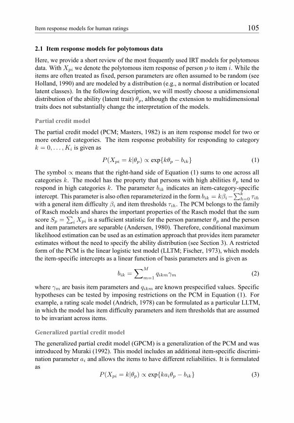
Item response models for human ratings 105
2.1 Item response models for polytomous data
Here, we provide a short review of the most frequently used IRT models for polytomous
data. WithXpi we denote the polytomous item response of person p to item i. While the
items are often treated as fixed, person parameters are often assumed to be random (see
Holland, 1990) and are modeled by a distribution (e.g., a normal distribution or located
latent classes). In the following description, we will mostly choose a unidimensional
distribution of the ability (latent trait) θp, although the extension to multidimensionaltraits does not substantially change the interpretation of the models.
Partial credit model
The partial credit model (PCM; Masters, 1982) is an item response model for two or
more ordered categories. The item response probability for responding to category
k = 0, . . . ,Ki is given as
P (Xpi = k|θp) ∝ exp{kθp − bik} (1)
The symbol ∝ means that the right-hand side of Equation (1) sums to one across all
categories k. The model has the property that persons with high abilities θp tend torespond in high categories k. The parameter bik indicates an item-category-specific
intercept. This parameter is also often reparameterized in the form bik = kβi−∑k
h=0 τihwith a general item difficulty βi and item thresholds τih. The PCM belongs to the family
of Rasch models and shares the important properties of the Rasch model that the sum
score Sp =∑
iXpi is a sufficient statistic for the person parameter θp and the personand item parameters are separable (Andersen, 1980). Therefore, conditional maximum
likelihood estimation can be used as an estimation approach that provides item parameter
estimates without the need to specify the ability distribution (see Section 3). A restricted
form of the PCM is the linear logistic test model (LLTM; Fischer, 1973), which models
the item-specific intercepts as a linear function of basis parameters and is given as
bik =∑M
m=1qikmγm (2)
where γm are basis item parameters and qikm are known prespecified values. Specific
hypotheses can be tested by imposing restrictions on the PCM in Equation (1). For
example, a rating scale model (Andrich, 1978) can be formulated as a particular LLTM,
in which the model has item difficulty parameters and item thresholds that are assumed
to be invariant across items.
Generalized partial credit model
The generalized partial credit model (GPCM) is a generalization of the PCM and was
introduced by Muraki (1992). This model includes an additional item-specific discrimi-
nation parameter ai and allows the items to have different reliabilities. It is formulatedas
P (Xpi = k|θp) ∝ exp{kaiθp − bik} (3)

106 A. Robitzsch & J. Steinfeld
In most applications, the GPCM provides a better model fit than the PCM. Items with
larger item discriminations are preferred because they are more informative in discrim-
inating between persons with lower and higher ability values. As in the PCM, item
discriminations ai as well as item-category intercepts bik can be modeled as linear func-tions of the basis item parameters (Embretson, 1999); this makes the estimation of more
parsimonious models possible. It should be emphasized that the weighted sum score
Sp =∑
i aiXpi is a sufficient statistic for the person parameter θp.
Graded response model
The graded response model (GRM) proposed by Samejima (1969) belongs to the class
of so-called cumulative IRT models. The item response probabilities are given as
P (Xpi = k|θp) = G(aiθp−bi,k+1)−G(aiθp−bik) (bi0 = 0, bi,Ki+1 = ∞) (4)
where G is a link function that is typically the logistic link function or the probit link
function. The model includes item discriminations ai and ordered item intercepts bik.It is often found that the GRM and the GPCM provide similar fit to empirical datasets
(Forero & Maydeu-Olivares, 2009) and, hence, there are no crucial consequences of
choosing one of the two models. Again, the item parameters can be formulated as
linear functions to estimate restricted versions of the GRM. For the probit link function,
Equation (4) can be rewritten asX∗pi = aiθp+epi whereX
∗pi is an underlying continuous
variable for the ordinal itemXpi and epi is a standard, normally distributed residual. Theordinal item Xpi is obtained by discretizing the continuous variable X
∗pi with respect to
thresholds bik. Using the variable X∗pi has the advantage that correlated residuals can be
specified in the GRM, which can model violations of local independence. However, in
this situation, marginal maximum likelihood estimation is no longer computationally
feasible and limited information estimation procedures have to be applied (see Section
3).
Covariance structure model
The normal distribution is probably the most frequently applied distribution. Sometimes
the question arises whether the normal distribution can also be applied to ordinal items.
However, the probability density of the normal distribution is defined on the real line and
not on discrete values. Therefore, a misspecified model results if the normal distribution
is applied to ordinal items. The assumed normal density is given as
f(Xpi = k|θp) = (2πσi)− 1
2 exp{− (k − aiθp − µi)
2
2σ2i
}, i.e. Xpi = µi + aiθp + epi
(5)
An item i is parameterized with an item mean µi, an item discrimination ai, and aresidual variance σ2
i = V ar(epi). Unfortunately, the item parameters of the GPCM
or the GRM cannot be simply converted into the parameters of the normal distribution
in Equation (5). However, in some applications, the item and distribution parameters

Item response models for human ratings 107
from the covariance structure model (CSM; often referred to as confirmatory factor
analysis) shown in Equation (5) can be more easily interpreted than the parameters of
the GPCM or GRM. More formally, in a CSM, the mean vector µ = µ(γ) of the Iitems Xp1, . . . , XpI and the covariance matrix Σ = Σ(γ) are modeled as functionsof an unknown parameter vector γ (Bollen, 1989). In a CSM, the covariance matrix
is represented as Σ = ΛΦΛT + Ψ, where Λ is the loading matrix, Φ is the factor
covariance matrix andΨ is the residual covariance matrix. Then, the vector γ contains
elements of the mean vector, loadings and elements of the factor covariance, and residual
covariance matrices. When applied to ordinal data, the CSM is a so-called pseudo-
likelihood estimation approach as the assumed likelihood function is misspecified (Yuan
& Schuster, 2013). Interestingly, Arminger and Schoenberg (1989) showed that the mean
structure and the covariance structure in Equation (5) can be consistently estimated in
a confirmatory factor analysis based on a misspecified normal distribution for ordinal
items. However, so-called maximum likelihood robust standard errors should be used, in
order to ensure that valid statistical inferences can be made in the case of a misspecified
likelihood (White, 1982). Alternatively, the bootstrap resampling method of persons can
be used to obtain valid standard errors (Berk et al., 2014).
2.2 Many-facet rater model
The IRT models presented in the following paragraphs are based on virtual items of every
combination of an item and a rater (see Figure 1). We denote the corresponding item
responses as Xpir for person p to item i rated by rater r. Unidimensional many-facetrater models (MFRM) are obtained by applying the PCM, the GPCM, or the GRM to
these virtual items. The item response probability in the extension of the GPCM is given
as
P (Xpir = k|θp) ∝ exp{kairθp − bikr} (6)
and, for the GRM, it is written as
P (Xpir = k|θp) = G(airθp − bir,k+1)−G(airθp − birk) (7)
Typically, constrained versions of these models are applied to rating data. In the family
of Rasch models, the item discriminations air in the GPCM (Equation 6) are all set to
one (also labeled as Rasch-MFRM in the following). A Rasch-MFRM (Linacre, 1989)
imposes additional restrictions on item parameters such that
P (Xpir = k|θp) ∝ exp{kθp − kβi − kαr −∑k
h=0τih} (8)
In this specification, the parameter βi refers to the general item difficulty, αr is the rater
severity parameter and τih are item-step parameters. The model specified in Equation(8) is a particular LLTM of the PCM applied to virtual items with linear constraints on
item-category intercepts birk. It should be emphasized that rater effects are assumed tobe homogeneous across all items in Equation (8). An important extension to Equation

108 A. Robitzsch & J. Steinfeld
(8) is the introduction of further interaction effects between items and raters, which
allows for systematic item-specific rating behavior. The more restrictive model with
homogeneous rater effects can be tested against the more complex model that allows
for item-rater interactions. Rater centrality/extremity (see Wolfe, 2014) can be modeled
by including rater-step parameters αrh in Equation (8). We note that an identification
condition has to be assumed in order to estimate (8) (e.g., Σrαr = 0).
The Rasch-MFRM has the advantage that the unweighted sum score Sp = ΣirXpir
is a sufficient statistic for the person parameter θp. By using the many-facet Raschmodel as a scaling model for obtaining person parameter estimates, an implicit decision
about an equal weighting of items is made. From the perspective of item fit in real
data applications, items as well as raters will typically assess the person ability with
different precision. Therefore, an item response model that includes discrimination
parameters will almost always result in better model fit. Besides severity-leniency effects
or scale-usage effects of raters, raters can also differ in the reliability of the ratings they
provide. The item-rater discrimination parameter air is a measure of the reliability ofthe ratings of item i and rater r (M. Wu, 2017). A more parsimonious model, which
can also often be useful, linearly decomposes the item-rater discrimination, such that
air = ai + ar. Submodels that include only item discriminations (air = ai) or onlyrater discriminations (air = ar) provide further interesting diagnostic tools for studyingthe behavior of items and raters.
We emphasize that the GPCM (6) and the GRM (7) are often specified in a restricted
form in which item-rater parameters follow a linear function, such as in the LLTM. These
models are implemented in the R packages discussed in Section 3 of this paper.
2.3 Generalized many-facet rater model
As argued in the introduction, ratings are not locally independent across items and raters.
First, different raters evaluate the performance of a student on an item, which typically
introduces some dependency because additional item-specific factors besides general
ability are at play. Hence, an additional student-item interaction effect has to be modeled.
Second, the rating of one item by a rater can also influence the rating of another item by
the same rater (the halo effect). Therefore, an additional student-rater interaction needs
to be modeled. The MFRM can be extended to include these two additional random
effect parameters upi and vpr to model local dependence. The resulting generalizedmany-facet rater model (GMFRM; Wang et al., 2014; Verhelst & Verstralen, 2001, for a
version for dichotomous ratings) can be written as
P (Xpir = k|θp, upi, vpr) ∝ exp{kαiθp+kupi+kvpr−kβi−kαr−∑k
h=0τih} (9)
Several submodels of (9) can be estimated. A version of (9) that sets all item dis-
criminations ai to one is a multidimensional Rasch model (Wang et al., 2014) with
random person-item and person-rater effects. The size of the variance components
σ2i = V ar(upi) and σ
2r = V ar(vpr) quantifies the degree of the dependency of the

Item response models for human ratings 109
ratings. In some applications, it seems useful to include only the item or rater random
effect for local dependence. The GMFRM models the additional dependence caused by
ratings of the same items and by the same raters as additional random effects that prevent
the assumption of local independence. Alternatively, the GPCM (9) can be substituted by
a GRM using a latent variable representation. Using this approach, the random effects
can be integrated out so that only person ability appears as a person variable in the model
(Tuerlinckx & De Boeck, 2004; see also Ip, 2010). However, this equivalent model
introduces correlated residuals, as rating variables Xpir for the same item i and for thesame rater r are typically positively correlated. It must be emphasized that movingfrom the model with random effects to the equivalent model with correlated residuals
implies a change in the metric of item parameters because the ability metric has changed.
More formally, integrating out the random effects upi and vpr from (9) results in the
conditional response probability
P (Xpir = k|θp) ∝ exp{kλirαiθp − kλirβi − kλirαr −∑k
h=0λirτih (10)
with λir = (δ2σ2i + δ2α2
r + 1)12 }
where δ = 0.583 is a positive constant (see Ip, 2010). As the multiplication factorλir is always smaller than one, all item parameters are shrunken to the extent of local
dependence caused by person-item and person-rater interactions. Hence, comparisons of
the item parameters of the GMFRM and the MFRM should consider the transformation
formula in Equation (10) for item parameters. The size of the residual correlations in
(10) can also be computed based on the variance components of the random effects in
model (9).
2.4 Covariance structure model and generalizability theory
Instead of modeling the ordinal virtual items of the rating data with an item response
model for polytomous item responses, a CSM can alternatively be applied using normal
distributions for modeling the virtual itemsXpir. The mean structure can be represented
by general item effects and general rater effects for modeling severity. The covariance
structure can be modeled as a confirmatory factor modelΣ = ΛΦΛT +Ψ in which the
distribution parameters of person ability are represented in the covariance matrix Φ of
latent factors. Violations of local independence caused by ratings of the same items and
the same raters can be specified either as additional factors appearing in the covariance
matrix Φ or as a patterned residual covariance matrix Ψ. As argued above, the CSM
provides consistent estimates of the mean and covariance structure for ordinal items with
misspecified normal distribution likelihood (Arminger & Schoenberg, 1989). This also
holds true if the statistical models of G-theory (Brennan, 2001a) are applied to ordinal
items because these models are particular cases of CSMs.

110 A. Robitzsch & J. Steinfeld
2.5 Hierarchical rater model
The GFRM and the CSM model the dependency caused by rating the same items by
including an additional random effect or correlated residuals. Hierarchical rater models
(HRM; Patz et al., 2002; DeCarlo et al., 2011) assume the existence of a discrete true
rating ηpi of a person p on an item i. However, the true rating is not observed; rather, itis only indirectly measured by the ratings of several raters. The true rating categories
of all items serve as indicators of the person ability θp. As a consequence, the itemresponse ratings Xpir are hierarchically modeled, given true items ηpi, which are alsohierarchically modeled, given the person ability θp. At the first level, a probabilitydistribution P (Xpir = k|ηpi) specifies a rater model, while at the second level, thedistribution P (ηpi = η|θp) is specified. At the second level, the GPCM can be chosen
for modeling true ratings and can be written as
P (ηpi = η|θp) ∝ exp{ηαiθp − bik} (11)
For the rater model at the first level, two different model specifications have been
proposed in the literature. Patz et al. (2002) used a discretized normal distribution
as the rater model in the originally proposed hierarchical rater model (HRM; see also
Casabianca &Wolfe, 2017):
P (Xpir = k|ηpi) ∝ exp(− 1
2ψ2ir
[k − (ηpi + φir)]2)
(12)
The parameter φir represents a rater severity parameter that models the systematic
displacement of the ratings of rater r from the true rating ηpi. The variance parameterψir is a measure of the reliability of the rater. Large values for the variance represent
a high precision of the rater. The parameters φir and ψir can also be assumed to be
invariant across items if a more parsimonious model should be estimated. We want to
emphasize that (11) only parameterizes rater severity and rater imprecision. As noted by
Patz et al. (2002), the estimation of severities φir poses computational challenges forsmall rater-variances ψir.
DeCarlo et al. (2011) proposed a hierarchical rater model based on a latent class signal
detection model (HRM-SDT) in which the different scale usage of the raters can also be
modeled. The item response probabilities in the rater model are specified as a GRM:
P (Xpir = k|ηpi) = G(dirηpi − cir,k+1)−G(dirηpi − cirk) (13)
where dir are item-rater discriminations and cirk are item-rater-category thresholds.
Large values for dir represent highly discriminating raters. Rater severity/leniency orrater centrality/extremity is represented by different values of the thresholds cirk. Idealraters, who always agree with the true rating category η, have very large discriminationsdir (e.g., larger than 100) and item thresholds are given as cirk = dir × (k − 0.5). Itis evident that both hierarchical rater models take the dependence caused by rating the
same items into account. The HRM-SDT of DeCarlo et al. (2011) appears to be more

Item response models for human ratings 111
flexible in modeling different rater behavior than the HRM of Patz et al. (2002), although
it is possibly more difficult to estimate when only a small amount of data is available.
However, neither model takes into account the additional dependence structure that
occurs when multiple items are rated by one rater. If halo effects exist in applications,
the GMFRM or a model with correlated residuals could be used. Alternatively, the
hierarchical rater model can be extended to include an additional dependence structure
(see also Wang et al., 2014) or random person-rater effects.
3 Estimation methods and their implementation in R packages
In this section, we present a brief overview of estimation methods that can be used for the
rater models introduced in Section 2. We focus on the implementation of these methods
in a number of recently released R packages (R Core Team, 2018) written by the authors
(immer, Robitzsch & Steinfeld, 2018; TAM, Robitzsch, Kiefer, & Wu, 2018; sirt,Robitzsch, 2018b; LAM, Robitzsch, 2018a). This focus is intended to provide a basis
for the illustrative examples discussed later; it does not imply general recommendations
for real data analyses (see Rusch, Mair, & Hatzinger, 2013, for a more comprehensive
overview of R packages for IRT). In general, two broad classes can be distinguished:
maximum likelihood (ML) and Bayesian estimation. Several variants of ML estimation
are discussed (see also Holland, 1990).
Marginal maximum likelihood (MML) estimation (also labeled as full information maxi-
mum likelihood estimation, FIML) estimates model parameters under a distributional
assumption about person ability (and further random effects). In most cases, the normal
distribution is chosen for person ability. As person ability is a latent variable, it is inte-
grated out in the likelihood that the estimation problem can essentially be reduced to
estimating item parameters (and rater parameters) and person distribution parameters
(means, variances, and covariances). Essentially, MML operates under the assumption
of random persons. Therefore, a person distribution is described by a statistical model
and each person is not treated as a fixed entity for which the item response model holds.
The expectation maximization (EM) algorithm is often employed for MML estimation
(Aitkin, 2016). MML estimation for the Rasch-MFRM is available in the function
TAM::tam.mml.mfr() of the TAM package. Several submodels of the MFRM that
allow for different item discriminations can be estimated with TAM::tam.mml.2pl() orsirt::rm.facets(). An MML implementation of the HRM-SDT model of DeCarlo et
al. (2011) can be found in sirt::rm.sdt(). In principle, the HRM of Patz et al. (2002)
can also be estimated with the MML method, although an implementation is available in
any of the R packages discussed in this section. MML estimation for CSMs based on a
multivariate normal distribution can be found in the lavaan package (Rosseel, 2012) or
in the LAM::mlnormal() function. G-theory models have equal linear discriminationparameters and fall into the class of linear mixed effects models that can be estimated
with the lme4 package (Bates, Mächler, Bolker, & Walker, 2015).

112 A. Robitzsch & J. Steinfeld
In joint maximum likelihood (JML) estimation (Lord, 1980; also labeled as fixed ef-
fects estimation), person parameters and item parameters are estimated simultaneously.
Essentially, persons are treated as fixed and a single parameter is estimated for each
person. Hence, no distributional assumption of person ability is needed. The JML
estimation is only computationally stable for Rasch-MFRMs and is implemented in the
Facets software (Linacre, 1989, 2017). JML has the disadvantage that the number of
estimated parameters increases with the number of persons in the sample, which induces
the well-known bias in JML estimation (Andersen, 1980). For the PCM, a simple bias-
correction formula has been proposed (Andersen, 1980). However, this formula cannot
be easily generalized to rating data with complex rating designs in which the number of
ratings per person and per item differs. Considering the critique of JML in most of the
psychometric literature, resampling methods and analytical methods (Hahn & Newey,
2004) have been proposed, which practically remove the bias caused by JML estimation.
Bertoli-Barsotti, Lando, and Punzo (2014) proposed a modification to the likelihood
function of the Rasch model for JML estimation that removes most of the bias in item
parameters. The reason for the JML bias is that there is no simple way to handle persons
with extreme scores (persons score in the lowest category or in the largest category for
all items). The so-called ϵ-adjustment method of Bertoli-Barsotti et al. (2014) essentiallyapplies a linear function to the sum score Sp = ΣiXpi in order to map the interval [0,Mp](Mp is the maximum score for person p) onto [ϵ,Mp − ϵ]. It should be emphasized thatall scores are linearly transformed. The ϵ-adjustment approach is implemented in theimmer::immer_jml() function of the immer package (Robitzsch & Steinfeld, 2018)
and extends the method of Bertoli-Barsotti et al. (2014) to polytomous item responses and
multiple-matrix designs with arbitrary missing patterns. Therefore, this JML estimation
method with bias-correction enables the estimation of the Rasch-MFRM. The statistical
properties of the parameter estimates can be seen as being superior to alternative JML
implementations of the Rasch-MFRM (for example, in the Facets software; Linacre,
2017). Depending on the application, JML can be substantially faster than MML estima-
tion and, hence, JML could be seen as a viable estimation alternative even if persons are
treated as random.
Conditional maximum likelihood (CML; Andersen, 1980) estimation also avoids a
specification of the distribution of person ability as person parameters are completely
removed in the estimation approach. Hence, CML can be used under the perspective of
random persons as well as fixed persons. CML can only be applied for Rasch-MFRMs.
The basic idea of CML is that the likelihood of a particular item response pattern with
sum score v is conditioned on the sum of the likelihoods of all response patterns with
sum score v. It can be shown that the corresponding ratio is independent of personability and that CML provides consistent item parameter estimates (like MML estimates;
van der Linden, 1994). It should be emphasized that CML becomes cumbersome in
rating designs in which not all persons are rated by the same items and the same raters
because the CML computations must be separately evaluated for every missing data
pattern. CML for Rasch-MFRMs is available in the eRm package (Mair & Hatzinger,
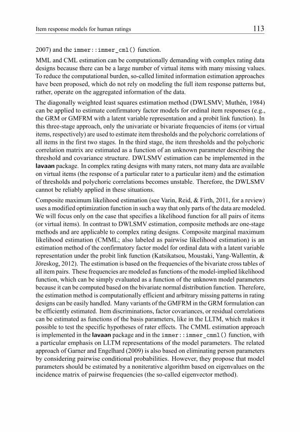
Item response models for human ratings 113
2007) and the immer::immer_cml() function.
MML and CML estimation can be computationally demanding with complex rating data
designs because there can be a large number of virtual items with many missing values.
To reduce the computational burden, so-called limited information estimation approaches
have been proposed, which do not rely on modeling the full item response patterns but,
rather, operate on the aggregated information of the data.
The diagonally weighted least squares estimation method (DWLSMV; Muthén, 1984)
can be applied to estimate confirmatory factor models for ordinal item responses (e.g.,
the GRM or GMFRM with a latent variable representation and a probit link function). In
this three-stage approach, only the univariate or bivariate frequencies of items (or virtual
items, respectively) are used to estimate item thresholds and the polychoric correlations of
all items in the first two stages. In the third stage, the item thresholds and the polychoric
correlation matrix are estimated as a function of an unknown parameter describing the
threshold and covariance structure. DWLSMV estimation can be implemented in the
lavaan package. In complex rating designs with many raters, not many data are available
on virtual items (the response of a particular rater to a particular item) and the estimation
of thresholds and polychoric correlations becomes unstable. Therefore, the DWLSMV
cannot be reliably applied in these situations.
Composite maximum likelihood estimation (see Varin, Reid, & Firth, 2011, for a review)
uses amodified optimization function in such a way that only parts of the data aremodeled.
We will focus only on the case that specifies a likelihood function for all pairs of items
(or virtual items). In contrast to DWLSMV estimation, composite methods are one-stage
methods and are applicable to complex rating designs. Composite marginal maximum
likelihood estimation (CMML; also labeled as pairwise likelihood estimation) is an
estimation method of the confirmatory factor model for ordinal data with a latent variable
representation under the probit link function (Katsikatsou, Moustaki, Yang-Wallentin, &
Jöreskog, 2012). The estimation is based on the frequencies of the bivariate cross tables of
all item pairs. These frequencies aremodeled as functions of themodel-implied likelihood
function, which can be simply evaluated as a function of the unknown model parameters
because it can be computed based on the bivariate normal distribution function. Therefore,
the estimation method is computationally efficient and arbitrary missing patterns in rating
designs can be easily handled. Many variants of the GMFRM in the GRM formulation can
be efficiently estimated. Item discriminations, factor covariances, or residual correlations
can be estimated as functions of the basis parameters, like in the LLTM, which makes it
possible to test the specific hypotheses of rater effects. The CMML estimation approach
is implemented in the lavaan package and in the immer::immer_cmml() function, witha particular emphasis on LLTM representations of the model parameters. The related
approach of Garner and Engelhard (2009) is also based on eliminating person parameters
by considering pairwise conditional probabilities. However, they propose that model
parameters should be estimated by a noniterative algorithm based on eigenvalues on the
incidence matrix of pairwise frequencies (the so-called eigenvector method).

114 A. Robitzsch & J. Steinfeld
As an alternative to CMML, a composite estimation method based on the CML principle
can be employed. Composite conditional maximum likelihood estimation (CCML)
evaluates the conditional likelihood for pairs of items. Hence, it is also based on only
the bivariate information of the dataset. The CCML approach has been proposed for the
LLTM for dichotomous data (Zwinderman, 1995) but it can be generalized to polytomous
items; our implementation can be found in the immer::immer_ccml() function. Tothis end, Rasch-MFRMs can be estimated more efficiently with CCML than with CML
in complex rating designs.
In recent years, Bayesian estimation approaches such as Markov chain Monte Carlo
(MCMC) have become very popular due to the availability of very flexible general
purpose Bayesian software programs such as BUGS, JAGS, or Stan. In a nutshell, the
MCMC approach is a simulation-based stochastic estimation algorithm, which uses
random draws of latent variables (person ability, random effects) and model parameters
conditional on the information contained in the dataset. The MCMC approach is often
seen as being computationally superior to ML estimation for IRT models with many
latent variables (Patz & Junker, 1999). In the GMFRM, the random effect person
ability as well as the person-item and person-rater effects are estimated. It is relatively
easy to estimate this model in a Gibbs sampling approach (Wang et al., 2014). The
immer package provides a wrapper function for the JAGS software (Plummer, 2003)in the immer::immer_gmfrm() function. The HRM of Patz et al. (2002) is mostly
estimated with MCMC methods although ML estimation is also possible (DeCarlo et
al., 2011). A Metropolis-Hastings within Gibbs sampling algorithm is employed in the
immer::immer_hrm() function.
It should be emphasized that MCMC estimates are asymptotically equivalent to ML
estimates. Hence, MCMC can also be used in applications without a primary focus on
Bayesian statistical inference. In IRT models for raters, informative prior distributions
decode prior knowledge about parameters in the Bayesian approach. Rater models are
often highly parameterized and researchers aim to avoid statistical overfitting. For exam-
ple, many item-specific rater effects are estimated in a rater model but only practically
relevant effects should be signaled by the model. An informative prior normal distribu-
tion with a mean of zero and a variance of 0.01 assumes that most rater effects are small.
Only those rater effects with large values are estimated as being significantly different
from zero (see Muthén &Asparouhov, 2012, for the application of prior distributions in
differential item functioning). In an alternative interpretation, model parameters are reg-
ularized in such a way that all nonsignificant effects are reduced to zero, which provides
a more focused view on the most relevant effects. Similarly, so-called penalized ML
estimation has been proposed as a regularization procedure under the ML paradigm for
assessing differential item functioning (Tutz & Schauberger, 2015). In the same manner,
rater effects can be regularized in a penalized ML approach of a Rasch-MFRM, which
will probably be implemented in the TAM package in the near future.

Item response models for human ratings 115
4 Choosing an appropriate rater model
The question of how to choose a suitable model involves an examination of the assump-
tions, expectations, and properties of the statistical models. In the following, we try to
provide a balanced view of advantages and disadvantages of the rater models presented
in Section 2.
It has been argued in Section 2 that typical rating designs imply the existence of local
dependence caused by person-item and person-rater interactions. While the GMFRM
deals with both sources of dependence, the HRM (either in the Patz et al., 2002 or the
HRM-SDT specification) only considers additional dependence caused by person-item
interactions. It can be argued that, for analytic ratings, halo effects (person-rater interac-
tions) play only a minor role and that therefore, the HRM often fits empirical datasets
sufficiently well. The GMFRM and HRM have the advantage that they typically provide
a good model (or are at least superior to the MFRM) and provide adequate reliability
estimates of person parameters, as sources of local dependence are explicitly modeled.
By applying one of the two model classes, a researcher puts substantial emphasis on
local dependence because the meaning of all of the model parameters (item parameters,
rater effects, and distribution parameters) is coupled with the modeled dependence. In
particular, the item and rater parameters in the GMFRM must be interpreted as being
conditional on person ability and random person-item and person-rater effects. If the
variances of the random item effects substantially differ from each other, item difficulties
can no longer be directly compared to each other because they operate on different
metrics. A comparison can be made if the random effects are integrated out to form
the conditional item response probabilities (see Section 2.3). In addition, the parallel
appearance of person ability and random item and rater effects in the GMFRM implies
that there is no unique (weighted) maximum likelihood estimator (WLE, Warm, 1989)
for the person parameter. Only the mean of the marginal posterior distribution (i.e.,
the expected value of the posterior distribution, EAP) can be used as a person ability
estimate. It should be noted that even in the case of equal discrimination parameters
in the GMFRM with random effects, the sum score is no longer a sufficient statistic of
the EAP because the ratings are weighted in such a way that ratings corresponding to
random effects with smaller variances receive larger weights, while random effects with
larger variances receive lower weights. Such a weighting scheme is not always favored,
especially in applications in which the person ability estimate is of vital importance for
the person itself (e.g., in feedback or in an examination). The HRM and GMFRM are
more computationally demanding than unidimensional rater models and this could be
seen as a disadvantage for practitioners. We think that this problem can be solved with
sufficient computational resources and is not a real limitation in the application of more
complex models.
Admittedly, the HRM and GMFRM can probably also not model aspects of the data
in order to describe the complex rating behavior. For example, raters can function
differently between persons (e.g., Eckes, 2005) or there could be rater drift during a

116 A. Robitzsch & J. Steinfeld
rating administration (e.g., Leckie & Baird, 2011). Persons are also often clustered within
organizational units (e.g., in universities, classes, courses, groups of peers, etc.). This
clustering induces additional dependence, which remains nonmodeled in the HRM or
GMFRM. However, these aspects are mostly not of major interest in statistical analysis
and will be considered as a nuisance (and therefore ignored in the statistical model).
Hence, a misspecified likelihood will almost always be the consequence, and pseudo-
likelihood estimation is essentially employed, which requires robust ML standard errors
(White, 1982). Model parameters resulting from pseudo-likelihood estimation can be
interpreted as estimates of some of the population parameters of an assumed statistical
model obtained by repeated sampling processes (of persons, raters, clusters, etc.) with
comparable assumptions.
In the Rasch-MFRM, the model parameters can be interpreted as being conditional on
person ability. The Rasch-MFRM models rater behavior by using a restricted PCM. It
has the advantage of computational simplicity as (bias-corrected) JML estimation is
computationally fast. Moreover, the sum score of the item responses of a person is a
sufficient statistic for the person parameter (WLE, MLE), which facilitates interpretation
because of the equal weighting of all the ratings. Rasch-MFRMs assume local stochastic
independence and therefore ignore possible dependencies caused by rating the same
items or ratings by the same raters. Interestingly, the assumption of local independence
in the application of a unidimensional item response model can essentially be reduced
to the assumption that residuals cancel out on average. This means that it is assumed
that positive and negative local dependence cancel each other out. This assumption is
defensible if person ability is interpreted as amajor dimension that is statistically extracted
from the dataset. Possible violations caused by local independence are regarded as a
nuisance factor in statistical modeling. If the sole argument for applying the HRM or the
GMFRM is to obtain correct standard errors or adequate reliability estimates for person
parameters, we think that this choice is unfounded and that the Rasch-MFRM should be
considered instead. The application of the Rasch-MFRM under the local independence
assumption should be contrasted with the GMFRM, in which the appearance of random
effects only allows for positive local dependence. The nonmodeled positive dependence
in the Rasch-MFRM implies that the reliability of the person parameters is underestimated
and, therefore, procedures correcting for local dependence have been proposed (Bock,
Brennan, & Muraki, 2002). With respect to model parameters such as item difficulties
or rater severity effects, robust ML standard errors should be used because the Rasch-
MFRM will typically employ a misspecified likelihood function. Notably, this pseudo-
likelihood estimation nevertheless provides consistent parameter estimates under repeated
sampling assumptions because, asymptotically, the (Kullback-Leibler) distance between
a true complex (and unknown) distribution and an assumed parameterized distribution
is minimized (White, 1982). As a consequence, the parameter estimates of the Rasch-
MFRM for different samples are only comparable (or can only be linked to each other)
if similar rating designs are employed that ensure that the extent of (ignored) local
dependence remains similar in different samples. When this condition is fulfilled, the use
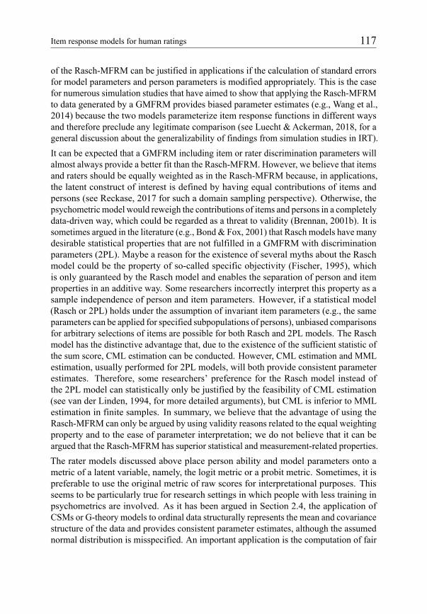
Item response models for human ratings 117
of the Rasch-MFRM can be justified in applications if the calculation of standard errors
for model parameters and person parameters is modified appropriately. This is the case
for numerous simulation studies that have aimed to show that applying the Rasch-MFRM
to data generated by a GMFRM provides biased parameter estimates (e.g., Wang et al.,
2014) because the two models parameterize item response functions in different ways
and therefore preclude any legitimate comparison (see Luecht & Ackerman, 2018, for a
general discussion about the generalizability of findings from simulation studies in IRT).
It can be expected that a GMFRM including item or rater discrimination parameters will
almost always provide a better fit than the Rasch-MFRM. However, we believe that items
and raters should be equally weighted as in the Rasch-MFRM because, in applications,
the latent construct of interest is defined by having equal contributions of items and
persons (see Reckase, 2017 for such a domain sampling perspective). Otherwise, the
psychometric model would reweigh the contributions of items and persons in a completely
data-driven way, which could be regarded as a threat to validity (Brennan, 2001b). It is
sometimes argued in the literature (e.g., Bond & Fox, 2001) that Rasch models have many
desirable statistical properties that are not fulfilled in a GMFRM with discrimination
parameters (2PL). Maybe a reason for the existence of several myths about the Rasch
model could be the property of so-called specific objectivity (Fischer, 1995), which
is only guaranteed by the Rasch model and enables the separation of person and item
properties in an additive way. Some researchers incorrectly interpret this property as a
sample independence of person and item parameters. However, if a statistical model
(Rasch or 2PL) holds under the assumption of invariant item parameters (e.g., the same
parameters can be applied for specified subpopulations of persons), unbiased comparisons
for arbitrary selections of items are possible for both Rasch and 2PL models. The Rasch
model has the distinctive advantage that, due to the existence of the sufficient statistic of
the sum score, CML estimation can be conducted. However, CML estimation and MML
estimation, usually performed for 2PL models, will both provide consistent parameter
estimates. Therefore, some researchers’ preference for the Rasch model instead of
the 2PL model can statistically only be justified by the feasibility of CML estimation
(see van der Linden, 1994, for more detailed arguments), but CML is inferior to MML
estimation in finite samples. In summary, we believe that the advantage of using the
Rasch-MFRM can only be argued by using validity reasons related to the equal weighting
property and to the ease of parameter interpretation; we do not believe that it can be
argued that the Rasch-MFRM has superior statistical and measurement-related properties.
The rater models discussed above place person ability and model parameters onto a
metric of a latent variable, namely, the logit metric or a probit metric. Sometimes, it is
preferable to use the original metric of raw scores for interpretational purposes. This
seems to be particularly true for research settings in which people with less training in
psychometrics are involved. As it has been argued in Section 2.4, the application of
CSMs or G-theory models to ordinal data structurally represents the mean and covariance
structure of the data and provides consistent parameter estimates, although the assumed
normal distribution is misspecified. An important application is the computation of fair
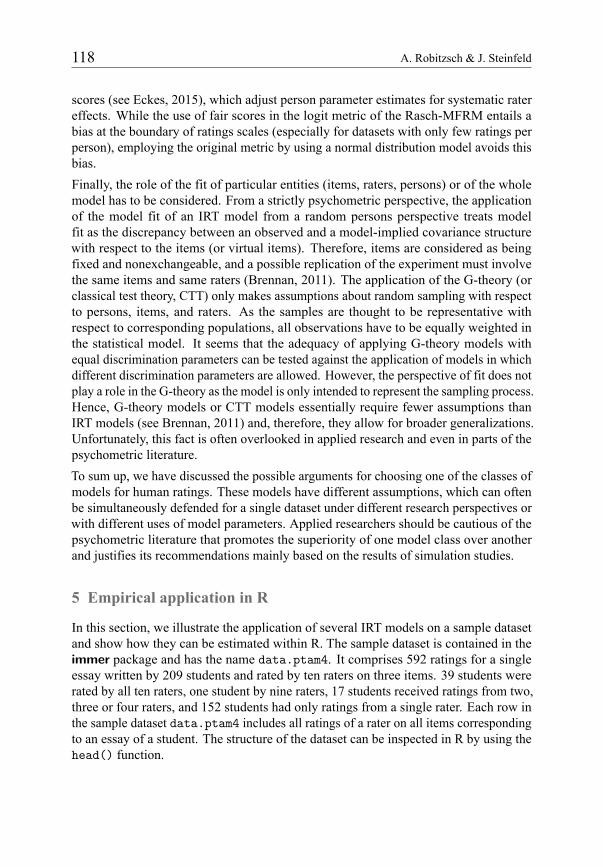
118 A. Robitzsch & J. Steinfeld
scores (see Eckes, 2015), which adjust person parameter estimates for systematic rater
effects. While the use of fair scores in the logit metric of the Rasch-MFRM entails a
bias at the boundary of ratings scales (especially for datasets with only few ratings per
person), employing the original metric by using a normal distribution model avoids this
bias.
Finally, the role of the fit of particular entities (items, raters, persons) or of the whole
model has to be considered. From a strictly psychometric perspective, the application
of the model fit of an IRT model from a random persons perspective treats model
fit as the discrepancy between an observed and a model-implied covariance structure
with respect to the items (or virtual items). Therefore, items are considered as being
fixed and nonexchangeable, and a possible replication of the experiment must involve
the same items and same raters (Brennan, 2011). The application of the G-theory (or
classical test theory, CTT) only makes assumptions about random sampling with respect
to persons, items, and raters. As the samples are thought to be representative with
respect to corresponding populations, all observations have to be equally weighted in
the statistical model. It seems that the adequacy of applying G-theory models with
equal discrimination parameters can be tested against the application of models in which
different discrimination parameters are allowed. However, the perspective of fit does not
play a role in the G-theory as the model is only intended to represent the sampling process.
Hence, G-theory models or CTT models essentially require fewer assumptions than
IRT models (see Brennan, 2011) and, therefore, they allow for broader generalizations.
Unfortunately, this fact is often overlooked in applied research and even in parts of the
psychometric literature.
To sum up, we have discussed the possible arguments for choosing one of the classes of
models for human ratings. These models have different assumptions, which can often
be simultaneously defended for a single dataset under different research perspectives or
with different uses of model parameters. Applied researchers should be cautious of the
psychometric literature that promotes the superiority of one model class over another
and justifies its recommendations mainly based on the results of simulation studies.
5 Empirical application in R
In this section, we illustrate the application of several IRT models on a sample dataset
and show how they can be estimated within R. The sample dataset is contained in the
immer package and has the name data.ptam4. It comprises 592 ratings for a singleessay written by 209 students and rated by ten raters on three items. 39 students were
rated by all ten raters, one student by nine raters, 17 students received ratings from two,
three or four raters, and 152 students had only ratings from a single rater. Each row in
the sample dataset data.ptam4 includes all ratings of a rater on all items correspondingto an essay of a student. The structure of the dataset can be inspected in R by using the
head() function.

Item response models for human ratings 119
It can be seen that the student with identifier (variable idstud) 10010 has two rowsin the dataset which means that she or he received ratings from two raters (variable
rater) 844 and 802. Ratings were provided on three items crit2, crit3 and crit4on a four-point scale (with integer values 0, 1, 2, and 3).
Complete syntax for the specification of all models in this section is provided by a
vignette which is included in the immer package.R> data(data.ptam4, package="immer")R> dat <- data.ptam4R> head(dat)
idstud rater crit2 crit3 crit41 10005 802 3 3 22 10009 802 2 2 13 10010 844 0 1 24 10010 802 2 2 15 10014 837 1 2 26 10014 824 0 2 2
Item response models for a single item
Before analyzing the complete rating dataset with three items, we investigate rater effects
based on only a single item “crit2”. We use a dataset in a so called wide format in which
columns refer to ratings of a single rater. In our analysis, we use ratings of 40 students
who received multiple ratings from ten raters. Only one student was unintentionally
rated by only nine raters. The dataset can be attached as data.ptam4wide from the
immer package.Table 1:
Descriptive Statistics for Item “crit2”
Rater Cat0 Cat1 Cat2 Cat3 M SD Cor
R802 .10 .38 .38 .15 1.58 0.87 .76
R803 .33 .38 .18 .13 1.10 1.01 .79
R810 .20 .38 .33 .10 1.33 0.92 .86
R816 .25 .25 .35 .15 1.40 1.03 .80
R820 .03 .46 .38 .13 1.62 0.75 .69
R824 .23 .40 .25 .13 1.28 0.96 .78
R831 .18 .33 .35 .15 1.48 0.96 .87
R835 .38 .28 .23 .13 1.10 1.06 .76
R837 .08 .30 .35 .28 1.83 0.93 .79
R844 .30 .25 .25 .20 1.35 1.12 .78
Note: Cat0, Cat1, Cat2, Cat3 = relative frequencies for categories 0, 1, 2, 3; Cor = correlation of rating of a
single rater with average score across all raters
Table 1 displays descriptive statistics for the rating dataset for item “crit2”. Category
frequencies, the mean, the standard deviation and the correlation of a rating with the aver-

120 A. Robitzsch & J. Steinfeld
age score across all ratings are shown in the table. By comparing the means, it is evident
that Raters 803 and 835 are severe while Rater 837 is lenient. Moreover, by inspecting
relative frequencies and the standard deviations, Rater 820 shows a centrality tendency
while Rater 844 can be characterized by an extremity tendency. Finally, by considering
the correlation with the average score, Rater 820 exhibits the lowest agreement, while
Raters 810 and 831 show the largest extent of agreement.
In the next step, we apply several item response models to the rating dataset involving
the single item “crit2” (see Wolfe, 2014, M. Wu, 2017 for applications of this approach).
In this approach, an item refers to a single rater and each rater is parameterized by its own
set of parameters. First, it is assumed that a continuous variable is used for modelling the
ratings of the four-point scale item. We fit the PCM with an assumption of homogeneous
rater effects (i.e., all raters possess the same set of parameters), the PCM, and the GPCM
(Models M01, M02, and M03). Second, we follow the principle of the HRM in which
true ratings of an item are modelled. Therefore, we specify located latent class Rasch
models (LOCLCA; Formann, 1985) which parameterize the response functions of the
raters by the PCM but assume a discrete ability variable. The locations of these latent
classes on the θ metric and the class probabilities are estimated. In our analysis, we fitLOCLCA with three, four and five latent classes (Models M13, M14, and M15). For
the four-point scale item, a LOCLCA with four latent classes would be expected if true
ratings can be empirically identified.
Table 2:
Model Comparisons for Item Response Models for Item “crit2”
Label Model Deviance #par AIC BIC
M01 PCM equal 861.03 4 869 876
M02 PCM 785.58 31 848 900
M03 GPCM 774.45 40 854 922
M13 LOCLCA(3) 808.14 34 876 934
M14 LOCLCA(4) 775.52 36 848 908
M15 LOCLCA(5) 769.24 38 845 909
Note: #par = number of estimated parameters; PCM equal = partial credit model in which parameters for all
raters were constrained to be equal; LOCLCA(k) = Located class analysis with k located latent classes and the
PCM is used as the item response function.
Table 2 contains deviances and information criteria for the fitted models. Model selection
can be conducted by using differences of deviance values of nestedmodels and performing
a likelihood ratio test (LRT) or by considering models with smallest information criteria
AIC and BIC. When comparing models M01, M02 and M03, it turned out that the model
with equal parameters for raters must be rejected which means that raters differ with
respect to their rating behavior. The GPCM did not fit the data significantly better than
the PCM although the small sample size (N = 40) has to be considered. As an example,we show how to fit the PCM using the TAM package and discuss parts of the summary

Item response models for human ratings 121
output (dat2 is the dataset data.ptam4wide).R> items <- c("crit2","crit3","crit4")R> mod02 <- TAM::tam.mml( resp=dat2[,items] , irtmodel="PCM2")R> summary(mod)
Item Parameters -A*Xsiitem N M xsi.item AXsi_.Cat1 AXsi_.Cat2 AXsi_.Cat3 B.Cat1.Dim1
1 R802 40 1.425 0.274 -2.923 -2.414 0.823 12 R803 40 1.300 0.714 -1.033 -0.730 2.142 13 R810 40 1.500 -0.086 -2.960 -2.047 -0.257 14 R816 40 1.600 -0.401 -3.892 -3.814 -1.203 15 R820 39 1.513 -0.011 -4.095 -3.747 -0.033 16 R824 40 1.450 0.333 -2.867 -2.745 0.998 17 R831 40 1.425 0.180 -2.263 -1.177 0.540 18 R835 40 1.450 0.228 -3.922 -3.602 0.683 19 R837 40 2.075 -2.073 -5.491 -7.872 -6.219 110 R844 40 1.600 -0.199 -2.812 -2.944 -0.597 1
The argument irtmodel="PCM2" requests the Andrich (1978) parameterization of thePCM. The column xsi.item contains the item difficulty of the PCM which can be
interpreted as rater severity/leniency. The most lenient Rater 837 has the smallest item
difficulty (i.e., rater difficulty) while for the most severe Rater 803 the largest parameter
was obtained. The columns AXsi_.Cat1, AXsi_.Cat2 and AXsi_.Cat3 include rater-category parameters which assess aspects of severity/leniency or centrality/extremity
behavior of the raters. The rater parameters can most easily be interpreted by computing
Thurstonian thresholds from the PCM using the TAM::tam.threshold() function.
Rater
Logi
t
R802 R803 R810 R816 R820 R824 R831 R835 R837 R844
−4
−2
02
4
−4
−2
02
4
Cat 0−>1 Cat 1−>2 Cat 2−>3
Figure 2:
Rater thresholds from the PCM (Model M02)
In Figure 2, the thresholds for all raters and all categories are depicted. It is evident that

122 A. Robitzsch & J. Steinfeld
Raters 802 and 837 are lenient with respect to using the zero category while the opposite
is true for Rater 835. Summing up, it can be seen that the variability of the thresholds
among raters between 0 and 1 is much larger than for the thresholds between 1 and 2
and 2 and 3. This means that the raters show less agreement for rating students in lower
categories, but more agreement in rating higher categories.
We also compute infit statistics for raters (Eckes, 2015) based on the PCM (Model
M02) using the TAM::msq.itemfit() function. Raters 810 and 831 which showed thehighest agreement with the average rating (see Table 1) have the lowest infit statistics
(.77 and .75, respectively) which can be interpreted as overfit. The largest infit statistics
were observed for Raters 835 and 844 (1.14 and 1.19, respectively) which indicates
underfit of these two raters. The GPCM can be fitted using the TAM::tam.mml.2pl()function using the argument irtmodel="GPCM". It turned out that Raters 810 and 831have the largest rater discriminations (4.25 and 4.39, respectively).
The model fit for different LOCLCAs are shown in Table 2. It should be emphasized
that the LOCLCA with four or five latent classes has a slightly superior fit to the PCM
which assumes a continuous ability. Although the LOCLCA with four classes could be
preferred because it can be more easily interpreted, we present the results of the LOCLCA
with five classes. The LOCLCA can be fitted using the TAM::tamaan() function whichallows the specification of IRT models similarly to the lavaan package.
R> tammodel <- "R+ ANALYSIS:R+ TYPE=LOCLCA; # type of the modelR+ NCLASSES(5); # 5 classesR+ NSTARTS(10,30); # 10 random starts with 30 iterationsR+ LAVAAN MODEL:R+ F =~ R802__R844R+ "R> mod15 <- TAM::tamaan( tammodel , resp=dat2 )R> summary(mod)
Cluster locationsV1 prob
Cl1 -9.990 0.048Cl2 -2.814 0.108Cl3 -0.124 0.334Cl4 1.463 0.335Cl5 3.415 0.175------------------------------------------------------------Item Response Probabilities
item itemno Cat Class1 Class2 Class3 Class4 Class51 R802 1 0 0.9988 0.3835 0.0284 0.0024 0.00002 R802 1 1 0.0012 0.5975 0.6526 0.2641 0.02423 R802 1 2 0.0000 0.0190 0.3056 0.6048 0.39034 R802 1 3 0.0000 0.0001 0.0133 0.1288 0.5855
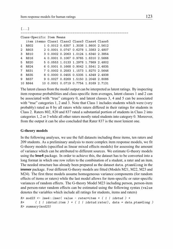
Item response models for human ratings 123
[...]------------------------------------------------------------Class-Specific Item Means
item itemno Class1 Class2 Class3 Class4 Class51 R802 1 0.0012 0.6357 1.3038 1.8600 2.56122 R803 2 0.0001 0.0747 0.6278 1.3383 2.48073 R810 3 0.0002 0.2063 1.0124 1.6340 2.38544 R816 4 0.0001 0.1067 0.9765 1.8310 2.56665 R820 5 0.0553 1.0133 1.2978 1.7869 2.48026 R824 6 0.0001 0.1668 0.9042 1.5541 2.48357 R831 7 0.0002 0.2583 1.1573 1.8270 2.56468 R835 8 0.0000 0.0455 0.5335 1.4349 2.49389 R837 9 0.0027 0.8269 1.5150 2.2048 2.808610 R844 10 0.0001 0.0719 0.7754 1.8169 2.7131
The latent classes from themodel output can be interpreted as latent ratings. By inspecting
item response probabilities and class-specific item averages, latent classes 1 and 2 can
be associated with “true” category 0, and latent classes 3, 4 and 5 can be associated
with “true” categories 1, 2 and 3. Note that Class 1 includes students which were (very
probably) rated as 0 by all raters while raters differed in their ratings for students in
Class 2. Raters 802, 820 and 837 rated a substantial portion of students in Class 2 into
categories 1, 2 or 3 while all other raters mostly rated students into category 0. Moreover,
from the output it can be also concluded that Rater 837 is the most lenient one.
G-theory models
In the following analyses, we use the full datasets including three items, ten raters and
209 students. As a preliminary analysis to more complex item response models, we fit
G-theory models (specified as linear mixed effects models) for assessing the amount
of variance which can be attributed to different sources. We estimate G-theory models
using the lme4 package. In order to achieve this, the dataset has to be converted into a
long format in which one row refers to the combination of a student, a rater and an item.
The needed structure has already been prepared as the dataset data.ptam4long in theimmer package. Four different G-theory models are fitted (Models M21, M22, M23 and
M24). The first three models assume homogeneous variance components (for random
effects of items or raters) while the last model allows for item-specific or rater-specific
variances of random effects. The G-theory Model M23 including person, person-item
and person-rater random effects can be estimated using the following syntax (valuedenotes the variables which include all ratings for students, items and raters)
R> mod23 <- lme4::lmer( value ~ rater*item + ( 1 | idstud ) +R+ ( 1 | idstud:item ) + ( 1 | idstud:rater), data = data.ptam4long )R> summary(mod23)

124 A. Robitzsch & J. Steinfeld
Random effects:Groups Name Variance Std.Dev.idstud:item (Intercept) 0.06497 0.2549idstud:rater (Intercept) 0.09344 0.3057idstud (Intercept) 0.28119 0.5303Residual 0.21512 0.4638
Number of obs: 1776, groups: idstud:item, 627; idstud:rater, 592; idstud, 209
In this model, rater-specific item means are allowed (fixed effects item*rater). It canbe seen from the output that a large part of the variance corresponds to student ability.
Interestingly, the variance component due to person-rater interactions (i.e., halo effects)
is slightly larger than the amount of dependence due to person-item interactions. This
finding sheds some light on the application of HRM which only handles dependency
due to random item effects but not to random rater effects.
Table 3:
Variance Component Estimates from G-theory Models
Variance Model M21 Model M22 Model M23
p .331 .323 .281
p× i — .044 .065
p× r — — .093
Residual .334 .299 .215
Note: p = persons; i = items; r = raters
In Table 3, the variance component estimates for the first three models are shown. When
comparing Model M21 and M22, it can be seen that most part of the variance of the item
effect (p× i) is confounded with the residual variance in Model M21. When including
the random rater effect (p× r) in Model 23, a substantial part of the true score variance
is captured which shows that neglecting dependency due to halo effects results in overly
optimistic reliability estimates because the true score variance is overestimated.
Finally, we show how to estimate a G-theory model with heterogeneous variance compo-
nents (Model M24). The specification is a bit cumbersome when done manually because
dummy variables for all items (e.g., I_crit2) and all raters (e.g., R_802) are involvedin the model specification.
R> mod24 <- lme4::lmer( value ~ rater * item + (1 | idstud) +R+ (0 + I_crit4 | idstud:item) + (0 + I_crit3 | idstud:item) +R+ (0 + I_crit2 | idstud:item) + (0 + R_844 | idstud:rater) +R+ (0 + R_837 | idstud:rater) + (0 + R_835 | idstud:rater) +R+ (0 + R_831 | idstud:rater) + (0 + R_824 | idstud:rater) +R+ (0 + R_820 | idstud:rater) + (0 + R_816 | idstud:rater) +R+ (0 + R_810 | idstud:rater) + (0 + R_803 | idstud:rater) +R+ (0 + R_802 | idstud:rater), data= data.ptam4long)
The variance component estimates of person-item interactions (idstud:item) wereestimated as .094 (Item “crit2”), .000 (Item “crit3”) and .092 (Item “crit4”) showing that

Item response models for human ratings 125
no local dependency was introduced for “crit3”. The variance component estimates of
person-rater interactions (idstud:rater) showed a considerable amount of variation(M= .096, SD=.059, Min=.027, Max=.204).
Many-facet rater models
In this subsection, we illustrate the application of several MFRMs. In a first series
of models, we fit Rasch-MFRMs which assume equal item and rater discrimination
parameters (Models M31, ..., M36). In a second series of models, we fit MFRMs which
allow the inclusion of item and rater discrimination parameters (Models M41, ..., M46).
In a Rasch-MFRM, the item response function for person p, item i, rater r and categoryk is given as P (Xpir = k|θp) ∝ exp(kθp − birk). Different constrained versions forparameters birk can be estimated. These versions can be defined using design matrices or– more conveniently – using the formula language in R when fitting Rasch-MFRMs with
the TAM::tam.mml.mfr() function in the TAM package. For example, the formula ~item*step + rater for facets items, raters and steps (i.e., categories) corresponds tothe constraint birk = bik + br. In principle, formulas of arbitrary complexity and anarbitrary number of facets can be specified in the TAM package using the argument
formulaA. The Rasch-MFRM ~ item*step + rater (Model M32) can be estimated
using the following syntax (dat is the dataset data.ptam4)R> facets <- dat[, "rater", drop=FALSE ]R> mod32 <- TAM::tam.mml.mfr( dat[,items], facets=facets,R+ formulaA = ~ item*step + rater, pid=dat$pid )R> summary(mod32)
Item Facet Parameters Xsi[...]7 rater802 rater -0.118 0.1018 rater803 rater 1.247 0.1019 rater810 rater -0.052 0.09910 rater816 rater -0.017 0.10111 rater820 rater -0.412 0.09912 rater824 rater 0.024 0.09913 rater831 rater 0.169 0.10014 rater835 rater 0.666 0.10015 rater837 rater -1.483 0.09916 rater844 rater -0.023 0.300[...]
The function automatically creates virtual items for estimating the constrained PCM.
The estimated item and rater parameters can be found in output section Item FacetParameters Xsi (only rater parameters are displayed). The main rater effects in thissection indicate the extent of leniency/severity tendencies. These rater effects are almost
perfectly correlated with the means for each rater (across all items) which can be expected
because these means are sufficient statistics for the rater effects.

126 A. Robitzsch & J. Steinfeld
Table 4:
Model Comparisons of Different Rasch-MFRMs
Label formulaA Deviance #par AIC BIC
M31 ~ item*step 3802.42 10 3822 3866
M32 ~ item*step+rater 3763.23 19 3801 3885
M33 ~ item*step+rater*step 3693.46 37 3767 3930
M34 ~ item*step+rater*item 3699.89 37 3774 3936
M35 ~ item*step+rater*item+rater*step 3632.30 55 3742 3983
M36 ~ item*rater*step 3562.38 91 3744 4143
Note: formulaA = formula specification of Rasch-MFRM; #par = number of estimated parameters.
In Table 4, model comparisons of different Rasch-MFRMs are shown. It can be seen that
model fit improves when interaction effects of raters and items or raters and categories
are included. The most complex model which assumes a PCM for all virtual items based
on combinations of items and raters would be favored based on a LRT but not based on
information criteria. It should be noted that information criteria are not to be expected to
provide valid statistical inference in case of incomplete designs1. This finding highlights
that the specification of rater models should not stop with modelling severity/leniency
tendencies as other rater effects can be of similar or larger importance.
In a second series of models, we investigate whether differences in discriminations
of items or raters can be found. Based on the item response function P (Xpir =k|θp) ∝ exp(kairθp − birk), different specifications for the discrimination parame-ter air are employed. These models can be estimated using the sirt::rm.facets()function. Different specifications for the discrimination parameters can be requested
by using the arguments est.a.item and est.a.rater. The following syntax showshow to estimate Model M44 (see also Table 5) which includes item and rater discrim-
inations in a multiplicative way (i.e., air = aiar). A model based on virtual items in
which all PCM (or GPCM) parameters are estimated can be requested by the argument
rater_item_int=TRUE.R> mod44 <- sirt::rm.facets( dat[ , items], rater=dat$rater, pid=dat$pid,R+ est.a.item=TRUE, est.a.rater=TRUE, reference_rater="831",R+ rater_item_int=FALSE)R> summary(mod44)
Item Parametersitem N M tau.Cat1 tau.Cat2 tau.Cat3 a delta delta_cent
1 crit2 592 1.409 -2.244 -2.053 0.542 0.889 0.181 0.368
1A large fraction of students in the dataset only received a single rating. With three items on a four-point scale,
10 parameters can be estimated for these students (9 item parameters and 1 variance parameter). However,
in the Rasch-MFRM specification all students are penalized in the AIC formula by the total number of
parameters which refers to a response pattern for students which have received multiple markings from all
raters (90 item parameters, 1 variance parameter). Therefore, the number of estimated parameters in the
AIC formula must be an overestimate of penalization in incomplete designs.

Item response models for human ratings 127
2 crit3 592 1.586 -5.166 -5.702 -1.675 1.475 -0.558 -0.3713 crit4 592 1.508 -3.342 -3.299 -0.555 0.762 -0.185 0.003-----------------------------------------------------------------Rater Parameters
rater N M b a thresh b.cent a.cent1 802 174 1.540 0.147 0.989 0.146 0.095 1.0532 803 183 1.158 0.959 1.263 1.211 0.906 1.3273 810 183 1.508 -0.306 0.972 -0.298 -0.358 1.0364 816 171 1.503 0.264 0.972 0.257 0.212 1.0355 820 180 1.606 -0.544 0.862 -0.469 -0.597 0.9266 824 189 1.492 0.129 1.093 0.141 0.077 1.1577 831 177 1.446 0.000 1.000 0.000 -0.052 1.0648 835 171 1.298 0.782 0.605 0.473 0.730 0.6699 837 180 1.944 -1.049 0.626 -0.656 -1.101 0.69010 844 168 1.512 0.140 0.980 0.137 0.088 1.044
From the output, we see that item “crit3” is more discriminative than the other two items
(see column a). Further, Raters 803 and 824 are most discriminative (i.e., accurate) whileRaters 835 and 837 are least discriminative (i.e., inaccurate) (see column a.cent). We
also calculated rater infit statistics from the Rasch-MFRMModel M32 (~ item*step +rater) and compared these with rater discriminations fromModel M42 (birk = bik+br,air = ar). Lower rater discriminations tended to result in higher rater infit values(r = −.33). It turned out that the relationship of both statistics was stronger (r = −.59)when an outlying observation (Rater 803) was removed from the calculation.
Table 5:
Model Comparisons of Different MFRMs
Label birk air Deviance #par AIC BIC
M41 bik + br 1 3763.23 18 3799 3878
M42 bik + br ar 3738.55 26 3791 3905
M43 bik + br ai 3750.96 20 3791 3879
M44 bik + br aiar 3724.43 29 3782 3910
M45 birk 1 3699.89 37 3774 3936
M46 birk air 3609.85 64 3738 4018
Note: bir = specification of item-specific rater intercept; air = specification of item-specific rater
discrimination #par = number of estimated parameters.
Finally, the model comparison from Table 5 indicated that the most flexible model
parameterizing all virtual items by the GPCM would be preferred based on the LRT
and AIC. In summary, it can be concluded that Rasch-MFRMs allowing for interaction
effects of raters with item or categories or MFRMs with rater discriminations should be
preferred from the perspective of model fit to a Rasch-MFRM in which only a main rater
severity effect is modelled. We expect that this conclusion will not change if measures
of approximate model fit would be employed. This modelling exercise illustrates our
argument that a preference of a simpler Rasch-MFRM can (in most applications) only be

128 A. Robitzsch & J. Steinfeld
justified for validity reasons, that is, when the differential weighting of items and raters
by a psychometric model is not warranted.
Generalized many-facet rater models
By employing G-theory models it was observed that there is a substantial amount of
variance attributed to person-item and person-rater interactions. Now, a series of GFRMs
is fitted in which we allowed item discriminations and we included particular variance
components. Four models were specified. Model M51 only contains the random person
effect. Model M52 additionally includes the random item effect while in Model M53
the random rater effect is included. Finally, we include all three variance components in
ModelM54. The immer package provides a wrapper function immer::immer_gmfrm()to the JAGS software (Plummer, 2003). Model M54 can be estimated using the following
syntax.
R> mod54 <- immer::immer_gmrfm(dat[,items], rater=dat$rater, pid=dat$idstud,R+ fe_r="r", re_pi=TRUE, re_pr=TRUE, iter=iter, burnin=burnin)
The argument fe_r specifies the fixed effects structure of intercepts birk of the IRTmodel with respect to raters. Options are "n" (birk = bik), "r" (birk = bik + br), "ir"(birk = bik + bir), "rk" (birk = bik + brk) or "a" (all effects are specified, i.e. all birkare estimated without constraints). The arguments re_pi and re_pr indicate whetherrandom effects should be included in the GMFRM. For example, Model M52 can be esti-
mated using re_pi=TRUE and re_pr=FALSE. We use 50,000 iterations (argument iter)and 10,000 burn-in iterations (argument burnin) which provided a good convergencebehavior of the MCMC estimation approach in our example.
We only briefly discuss the results of Model M54. The variance component estimates
varied considerably among items (“crit2”: .12, “crit3”: .05; “crit4”: .66). The rater
severities correlated highly with the average rater scores (r = −.99) and did also showsome variation among raters (SD=.48, Min=−1.06 [Rater 837], Max=0.84 [Rater 803]).The variance estimates for person-rater interactions also exhibited some variability
among raters (M=.27, SD=.32). Two Raters 844 (.53) and 803 (1.09) had remarkablyhigh variance estimates indicating that halo effects were strongly present for these raters.
Finally, the correlation of the rater variances from the GMFRM (Model M54) and from
the G-theory model (Model M24) was .84 indicating that findings remain relativelystable irrespectively of whether the logit or the original metric is chosen.
Hierarchical rater model based on signal detection theory
In the GMFRM, local dependence is taken into account by including additional random
effects. In the HRM, ratings are modelled by a hierarchical approach which first assumes
that manifest ratings are modelled conditionally on true discrete ratings (signal detection
model, SDM). Second, true ratings are modelled by item response functions (item
response model, IRM). For both models different specifications can be chosen.

Item response models for human ratings 129
Table 6:
Model Comparisons of Different HRM-SDT Models
Label IRM SDM Deviance #par AIC BIC
M61 PCM n 3540.53 10 3561 3594
M62 PCM e 3530.70 14 3559 3605
M63 PCM r 3314.19 50 3414 3581
M64 PCM a 3135.89 130 3396 3830
M71 GPCM n 3525.08 12 3549 3589
M72 GPCM e 3512.23 16 3544 3598
M73 GPCM r 3298.47 52 3402 3576
M74 GPCM a 3135.18 132 3399 3840
Note: IRM = specified item response model; SDM = specified signal detection model (n = no effects; e =
exchangeable effects for items and raters; r = rater effects; a = all effects); #par = number of estimated
parameters.
In Table 6, different specifications of our fittedmodels are shown. The IRMuses either the
PCM or the GPCM. In the SDM, discrimination parameters dir and intercept parameterscirk are estimated with several constraints. Regarding our sample dataset it turned outthe PCM with a SDM, in which all rater parameters were allowed to be item-specific,
showed the best fit (Model M64) in terms of the LRT and AIC.
For facilitating the interpretation, we focus on the discussion of results of Model M63 in
which rater effects in the SDM are assumed to be independent of items. The HRM-SDT
can be estimated using the sirt::rm.sdt() function. To choose the GPCM instead of
the PCM one has to use the argument est.a.item=TRUE. Different specifications ofthe SDM can be chosen by using the arguments est.c.rater and est.d.rater. Theestimation of Model M63 can be conducted using the following syntax.
R> mod63 <- sirt::rm.sdt( dat[,items], rater=dat$rater, pid=dat$idstud,R+ est.c.rater="r" , est.d.rater="r")R> summary(mod63)
Rater Parametersitem.rater N M d c_1 c_2 c_3 c_1.trans c_2.trans c_3.trans
1 crit2-802 58 1.655 4.939 2.590 7.356 13.000 0.524 1.489 2.6322 crit2-803 61 1.000 3.564 3.264 6.525 9.801 0.916 1.831 2.7503 crit2-810 61 1.344 4.529 1.213 6.819 11.463 0.268 1.506 2.5314 crit2-816 57 1.526 5.553 3.336 7.897 14.463 0.601 1.422 2.6055 crit2-820 60 1.650 7.967 -1.182 11.471 21.195 -0.148 1.440 2.6616 crit2-824 63 1.365 7.279 4.593 10.668 19.034 0.631 1.466 2.6157 crit2-831 59 1.373 4.509 1.449 7.464 11.728 0.321 1.655 2.6018 crit2-835 57 1.035 2.858 1.526 4.762 8.564 0.534 1.666 2.9969 crit2-837 60 1.833 2.857 -1.314 2.454 6.524 -0.460 0.859 2.28310 crit2-844 56 1.304 3.679 2.004 4.851 9.323 0.545 1.319 2.534
We focus on the interpretation of rater parameters. Raters 820 and 824 are most reliable

130 A. Robitzsch & J. Steinfeld
because high discrimination parameters dr were estimated for them. Further, Raters 835and 837 are least reliable. Severity/leniency and centrality/extremity tendencies can be
identified by the intercept parameters crk. The relative criteria locations c∗rk = crk/dr
(displayed as c_1.trans, c_2.trans, c_3.trans in the output) indicate the relative“difficulty” for every category of a rater. For raters which do not produce systematic
biases, relative criteria locations of .5, 1.5, and 2.5 would be expected for four-point
scale items. In Figure 3, these locations are displayed for all raters and all criteria. It
can be seen that Raters 820 and 837 are lenient with respect to rating students into the
zero category. Rater 803 is more severe because she or he more frequently rates students
into the zero category. The standard deviation among raters of relative criteria locations
can be computed to assess the uncertainty of rating particular categories. Differentiating
students between 0 and 1 showed most variability (SD=.40), while the SD for categories
1 and 2 (SD=.26) and 2 and 3 (SD=.18) was lower. It should be emphasized that ameasure of rater severity can be calculated from HRM-SDT output by averaging criteria
locations, i.e. computing c∗r =∑
k c∗rk/K.
Rater
c rk
d r
802 803 810 816 820 824 831 835 837 844
01
23
01
23
Cat 0−>1 Cat 1−>2 Cat 2−>3
4.9 3.6 4.5 5.6 8.0 7.3 4.5 2.9 2.9 3.7dr =
Figure 3: Plots of the relative criteria locations c∗rk = crk/dr for the HRM-SDT (Model M63).
The solid horizontal lines show intersection points for the underlying distributions.
Hierarchical rater model of Patz et al. (2002)
Finally, we want to fit the alternative HRM of Patz et al. (2002). This model includes rater
severity (rater bias) φir and rater variance ψir as rater parameters. Two models are fitted.
First, Model M81 assumes that the rater parameters are item independent while in Model
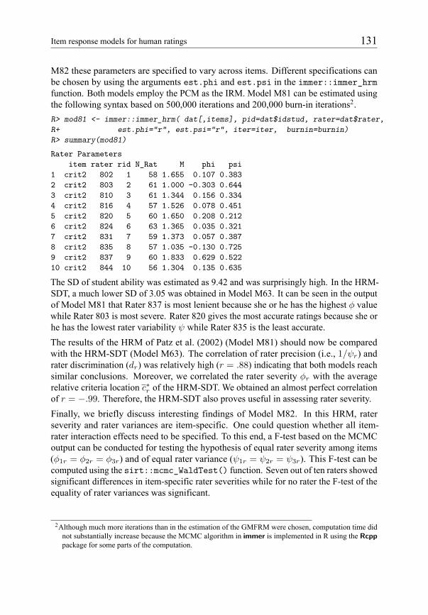
Item response models for human ratings 131
M82 these parameters are specified to vary across items. Different specifications can
be chosen by using the arguments est.phi and est.psi in the immer::immer_hrmfunction. Both models employ the PCM as the IRM. Model M81 can be estimated using
the following syntax based on 500,000 iterations and 200,000 burn-in iterations2.
R> mod81 <- immer::immer_hrm( dat[,items], pid=dat$idstud, rater=dat$rater,R+ est.phi="r", est.psi="r", iter=iter, burnin=burnin)R> summary(mod81)
Rater Parametersitem rater rid N_Rat M phi psi
1 crit2 802 1 58 1.655 0.107 0.3832 crit2 803 2 61 1.000 -0.303 0.6443 crit2 810 3 61 1.344 0.156 0.3344 crit2 816 4 57 1.526 0.078 0.4515 crit2 820 5 60 1.650 0.208 0.2126 crit2 824 6 63 1.365 0.035 0.3217 crit2 831 7 59 1.373 0.057 0.3878 crit2 835 8 57 1.035 -0.130 0.7259 crit2 837 9 60 1.833 0.629 0.52210 crit2 844 10 56 1.304 0.135 0.635
The SD of student ability was estimated as 9.42 and was surprisingly high. In the HRM-
SDT, a much lower SD of 3.05 was obtained in Model M63. It can be seen in the output
of Model M81 that Rater 837 is most lenient because she or he has the highest φ valuewhile Rater 803 is most severe. Rater 820 gives the most accurate ratings because she or
he has the lowest rater variability ψ while Rater 835 is the least accurate.
The results of the HRM of Patz et al. (2002) (Model M81) should now be compared
with the HRM-SDT (Model M63). The correlation of rater precision (i.e., 1/ψr) and
rater discrimination (dr) was relatively high (r = .88) indicating that both models reachsimilar conclusions. Moreover, we correlated the rater severity φr with the averagerelative criteria location c∗r of the HRM-SDT. We obtained an almost perfect correlation
of r = −.99. Therefore, the HRM-SDT also proves useful in assessing rater severity.
Finally, we briefly discuss interesting findings of Model M82. In this HRM, rater
severity and rater variances are item-specific. One could question whether all item-
rater interaction effects need to be specified. To this end, a F-test based on the MCMC
output can be conducted for testing the hypothesis of equal rater severity among items
(φ1r = φ2r = φ3r) and of equal rater variance (ψ1r = ψ2r = ψ3r). This F-test can be
computed using the sirt::mcmc_WaldTest() function. Seven out of ten raters showedsignificant differences in item-specific rater severities while for no rater the F-test of the
equality of rater variances was significant.
2Although much more iterations than in the estimation of the GMFRM were chosen, computation time did
not substantially increase because the MCMC algorithm in immer is implemented in R using the Rcpppackage for some parts of the computation.
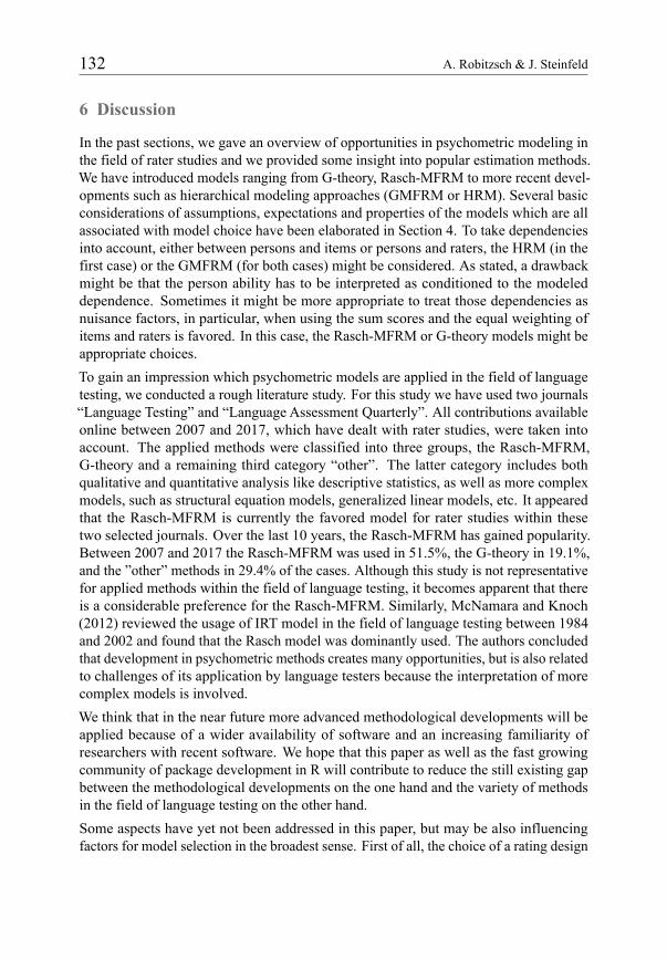
132 A. Robitzsch & J. Steinfeld
6 Discussion
In the past sections, we gave an overview of opportunities in psychometric modeling in
the field of rater studies and we provided some insight into popular estimation methods.
We have introduced models ranging from G-theory, Rasch-MFRM to more recent devel-
opments such as hierarchical modeling approaches (GMFRM or HRM). Several basic
considerations of assumptions, expectations and properties of the models which are all
associated with model choice have been elaborated in Section 4. To take dependencies
into account, either between persons and items or persons and raters, the HRM (in the
first case) or the GMFRM (for both cases) might be considered. As stated, a drawback
might be that the person ability has to be interpreted as conditioned to the modeled
dependence. Sometimes it might be more appropriate to treat those dependencies as
nuisance factors, in particular, when using the sum scores and the equal weighting of
items and raters is favored. In this case, the Rasch-MFRM or G-theory models might be
appropriate choices.
To gain an impression which psychometric models are applied in the field of language
testing, we conducted a rough literature study. For this study we have used two journals
“Language Testing” and “Language Assessment Quarterly”. All contributions available
online between 2007 and 2017, which have dealt with rater studies, were taken into
account. The applied methods were classified into three groups, the Rasch-MFRM,
G-theory and a remaining third category “other”. The latter category includes both
qualitative and quantitative analysis like descriptive statistics, as well as more complex
models, such as structural equation models, generalized linear models, etc. It appeared
that the Rasch-MFRM is currently the favored model for rater studies within these
two selected journals. Over the last 10 years, the Rasch-MFRM has gained popularity.
Between 2007 and 2017 the Rasch-MFRM was used in 51.5%, the G-theory in 19.1%,
and the ”other” methods in 29.4% of the cases. Although this study is not representative
for applied methods within the field of language testing, it becomes apparent that there
is a considerable preference for the Rasch-MFRM. Similarly, McNamara and Knoch
(2012) reviewed the usage of IRT model in the field of language testing between 1984
and 2002 and found that the Rasch model was dominantly used. The authors concluded
that development in psychometric methods creates many opportunities, but is also related
to challenges of its application by language testers because the interpretation of more
complex models is involved.
We think that in the near future more advanced methodological developments will be
applied because of a wider availability of software and an increasing familiarity of
researchers with recent software. We hope that this paper as well as the fast growing
community of package development in R will contribute to reduce the still existing gap
between the methodological developments on the one hand and the variety of methods
in the field of language testing on the other hand.
Some aspects have yet not been addressed in this paper, but may be also influencing
factors for model selection in the broadest sense. First of all, the choice of a rating design
Item response models for human ratings 133
should be emphasized. When choosing a rating design, there are a few possibilities which
reach from complete designs in which every rater judges every item to more sophisticated
incomplete designs which usually requires a kind of linking. Complete rating designs
are often not applicable for economic reasons that is why incomplete designs are chosen.
Several types of incomplete rating designs are possible; one of the more established ones
might be the practice of using common ratings. Here, a representative selection of persons
is rated by all raters, while the remaining ones are rated by one or more, but not by all
raters. Another possibility of rating designs which might reduce the venture of choosing
not representative common persons are overlap (or incomplete) designs (e.g. DeCarlo,
2010). Different types of overlap designs are feasible. All of them have in common that
decisions are required, which persons are allocated to rater, how many persons are rated
per rater, and how raters are linked among each other. These considerations or decisions
can themselves lead to additional effects (Casabianca &Wolfe, 2017).
Another yet not mentioned aspect of rater models is the development of automated
scoring systems, especially in the area of large-scale assessments. From an economical
point of view, this approach might be more efficient than human ratings although the
validity of automated scoring approaches can be questioned. It should be noted that the
discussion about choosing appropriate rater models for human raters is also important for
calibrating automated scoring systems because the calibration relies on human ratings
(Wind, Wolfe, Engelhard, Foltz, & Rosenstein, 2018).
Acknowledgment
We would like thank Thomas Eckes for stimulating us to contribute to this special issue,
and in particular for his consideration and very helpful feedback on previous versions of
the manuscript.
References
Aitkin, M. (2016). Expectation maximization algorithm and extensions. In W. van der Linden
(Ed.), Handbook of item response theory. Volume Two: Statistical Tools (pp. 217–236).
Boca Raton: CRC Press.
Andersen, E. B. (1980). Discrete statistical models with social science applications. Amsterdam:
North-Holland Publishing Co.
Andrich, D. (1978). A rating formulation for ordered response categories. Psychometrika, 43(4),
561–573.
Arminger, G., & Schoenberg, R. J. (1989). Pseudo maximum likelihood estimation and a test for
misspecification in mean and covariance structure models. Psychometrika, 54(3), 409–425.
Bates, D., Mächler, M., Bolker, B., &Walker, S. (2015). Fitting linear mixed-effects models using
lme4. Journal of Statistical Software, 67(1), 1–48.

134 A. Robitzsch & J. Steinfeld
Bechger, T. M., Maris, G., & Hsiao, Y. P. (2010). Detecting halo effects in performance-based
examinations. Applied Psychological Measurement, 34(8), 607–619.
Berk, R., Brown, L., Buja, A., George, E., Pitkin, E., Zhang, K., & Zhao, L. (2014). Misspec-
ified mean function regression: making good use of regression models that are wrong.
Sociological Methods & Research, 43(3), 422–451.
Bertoli-Barsotti, L., Lando, T., & Punzo, A. (2014). Estimating a Rasch model via fuzzy empirical
probability functions. In D. Vicari, A. Okada, G. Ragozini, & C. Weihs (Eds.), Analysis
and Modeling of Complex Data in Behavioral and Social Sciences (pp. 29–36). Cham,
Switzerland: Springer.
Bock, R. D., Brennan, R. L., & Muraki, E. (2002). The information in multiple ratings. Applied
Psychological Measurement, 26(4), 364–375.
Bollen, K. A. (1989). Structural equations with latent variables. New York: Wiley.
Bond, T. G., & Fox, C. M. (2001). Applying the Rasch model: Fundamental measurement in the
human sciences. Mahwah: Lawrence Erlbaum.
Brennan, R. L. (2001a). Generalizability theory. New York: Spinger.
Brennan, R. L. (2001b). Some problems, pitfalls, and paradoxes in educational measurement.
Educational Measurement: Issues and Practice, 20(4), 6–18.
Brennan, R. L. (2011). Generalizability theory and classical test theory. Applied Measurement in
Education, 24(1), 1–21.
Casabianca, J. M., &Wolfe, E.W. (2017). The impact of design decisions onmeasurement accuracy
demonstrated using the hierarchical rater model. Psychological Test and Assessment
Modeling, 59(4), 471–492.
De Boeck, P. (2008). Random item IRT models. Psychometrika, 73(4), 533–559.
DeCarlo, L. T. (2005). A model of rater behavior in essay grading based on signal detection theory.
Journal of Educational Measurement, 42(1), 53–76.
DeCarlo, L. T. (2010). Studies of a latent class signal detection model for constructed response scor-
ing II: Incomplete and hierarchical designs (ETS Research Report RR-10-08). Princeton:
ETS.
DeCarlo, L. T., Kim, Y., & Johnson, M. S. (2011). A hierarchical rater model for constructed
responses, with a signal detection rater model. Journal of Educational Measurement, 48(3),
333–356.
Eckes, T. (2005). Examining rater effects in TestDaF writing and speaking performance assess-
ments: A many-facet Rasch analysis. Language Assessment Quarterly, 2(3), 197–221.
Eckes, T. (2015). Introduction to many-facet Rasch measurement: Analyzing and evaluating
rater-mediated assessments (2nd ed.). Frankfurt am Main: Peter Lang.
Eckes, T. (2017). Guest Editorial Rater effects: Advances in item response modeling of human
ratings–Part I. Psychological Test and Assessment Modeling, 59(4), 443–452.

Item response models for human ratings 135
Embretson, S. E. (1999). Generating items during testing: Psychometric issues and models.
Psychometrika, 64(4), 407–433.
Engelhard, G. (1992). The measurement of writing ability with a many-faceted Rasch model.
Applied Measurement in Education, 5(3), 171–191.
Engelhard, G. (1994). Examining rater errors in the assessment of written composition with a
many-faceted Rasch model. Journal of Educational Measurement, 31(2), 93–112.
Fischer, G. H. (1973). The linear logistic test model as an instrument in educational research. Acta
Psychologica, 37(6), 359–374.
Fischer, G. H. (1995). Derivations of the Rasch model. In G. H. Fischer & I. W. Molenaar (Eds.),
Rasch models. foundations, recent developments, and applications (pp. 15–31). New York:
Springer.
Forero, C. G., & Maydeu-Olivares, A. (2009). Estimation of IRT graded response models: Limited
versus full information methods. Psychological Methods, 14(3), 275–299.
Formann, A. K. (1985). Constrained latent class models: Theory and applications. British Journal
of Mathematical and Statistical Psychology, 38(1), 87–111.
Garner, M., & Engelhard, G. (2009). Using paired comparison matrices to estimate parameters of
the partial credit Rasch measurement model for rater-mediated assessments. Journal of
Applied Measurement, 10(1), 30–41.
Hahn, J., & Newey, W. (2004). Jackknife and analytical bias reduction for nonlinear panel models.
Econometrica, 72(4), 1295–1319.
Holland, P. W. (1990). On the sampling theory foundations of item response theory models.
Psychometrika, 55(4), 577–601.
Ip, E. H. (2010). Empirically indistinguishable multidimensional IRT and locally dependent
unidimensional item response models. British Journal of Mathematical and Statistical
Psychology, 63(2), 395–416.
Katsikatsou, M., Moustaki, I., Yang-Wallentin, F., & Jöreskog, K. G. (2012). Pairwise likelihood
estimation for factor analysis models with ordinal data. Computational Statistics & Data
Analysis, 56(12), 4243–4258.
Leckie, G., & Baird, J.-A. (2011). Rater effects on essay scoring: A multilevel analysis of severity
drift, central tendency, and rater experience. Journal of Educational Measurement, 48(4),
399–418.
Linacre, J. (1989). Many-facet Rasch measurement. Chicago, IL: MESA Press.
Linacre, J. (2017). A user’s guide to FACETS: Rasch-model computer programs. Chicago:
Winsteps.com.
Lord, F. M. (1980). Applications of item response theory to practical testing problems. Mahwah,
New Jersey: Erlbaum.
Luecht, R., & Ackerman, T. A. (2018). A technical note on IRT simulation studies: Dealing
with truth, estimates, observed data, and residuals. Educational Measurement: Issues and

136 A. Robitzsch & J. Steinfeld
Practice, Advance online publication. doi: 10.1111/emip.12185
Lunz, M. E., Wright, B. D., & Linacre, J. M. (1990). Measuring the impact of judge severity on
examination scores. Applied Measurement in Education, 3(4), 331–345.
Mair, P., & Hatzinger, R. (2007). Extended Rasch modeling: The eRm package for the application
of IRT models in R. Journal of Statistical Software, 20(9), 1–20.
Masters, G. N. (1982). A Rasch model for partial credit scoring. Psychometrika, 47(2), 149–174.
McLaughlin, J. E., Singer, D., & Cox, W. C. (2017). Candidate evaluation using targeted construct
assessment in the multiple mini-interview: A multifaceted Rasch model analysis. Teaching
and Learning in Medicine, 29(1), 68–74.
McNamara, T., & Knoch, U. (2012). The Rasch wars: The emergence of Rasch measurement in
language testing. Language Testing, 29(4), 555–576.
Muraki, E. (1992). A generalized partial credit model: Application of an EM algorithm. Applied
Psychological Measurement, 16(1), 159–176.
Muthén, B. (1984). A general structural equation model with dichotomous, ordered categorical,
and continuous latent variable indicators. Psychometrika, 49(1), 115–132.
Muthén, B., & Asparouhov, T. (2012). Bayesian structural equation modeling: A more flexible
representation of substantive theory. Psychological Methods, 17(3), 313–335.
Myford, C. M., & Wolfe, E. W. (2003). Detecting and measuring rater effects using many-facet
Rasch measurement: Part I. Journal of Applied Measurement, 4(4), 386–422.
Patz, R. J., & Junker, B. W. (1999). Applications and extensions of MCMC in IRT: Multiple item
types, missing data, and rated responses. Journal of Educational and Behavioral Statistics,
24(4), 342–366.
Patz, R. J., Junker, B. W., Johnson, M. S., & Mariano, L. T. (2002). The hierarchical rater model
for rated test items and its application to large-scale educational assessment data. Journal
of Educational and Behavioral Statistics, 27(4), 341–384.
Plummer, M. (2003). JAGS: A program for analysis of Bayesian graphical models using Gibbs
sampling. Vienna,Austria: Proceedings of the 3rd International Workshop on Distributed
Statistical Computing (DSC 2003), March 20–22.
R Core Team. (2018). R: A language and environment for statistical computing. Austria: R
foundation for statistical computing Vienna.
Reckase, M. D. (2017). A tale of two models: Sources of confusion in achievement testing.
(Research Report No. RR-17-44). Princeton, NJ: Educational Testing Service.
Robitzsch,A. (2018a). LAM: Some latent variable models. R package version 0.2. https://CRAN.R-
project.org/package=LAM.
Robitzsch, A. (2018b). sirt: Supplementary item response theory models. R package version 2.5.
https://CRAN.R-project.org/package=sirt.
Robitzsch, A., Kiefer, T., & Wu, M. (2018). TAM: Test analysis modules. R package version 2.9.

Item response models for human ratings 137
https://CRAN.R-project.org/package=TAM.
Robitzsch, A., & Steinfeld, J. (2018). immer: Item response models for multiple ratings. R package
version 1.0. https://CRAN.R-project.org/package=immer.
Rosseel, Y. (2012). lavaan: An R Package for Structural Equation Modeling. Journal of Statistical
Software, 48(2), 1–36.
Rost, J., & Langeheine, R. (1997). A guide through latent structure models for categorical data. In
J. Rost & R. Langeheine (Eds.), Applications of latent trait and latent class models in the
social sciences (pp. 13–37). New York: Waxmann.
Rusch, T., Mair, P., & Hatzinger, R. (2013). Psychometrics with R: A review of CRAN packages
for item response theory. WU Vienna University of Economics and Business.
Saal, F. E., Downey, R. G., & Lahey, M.A. (1980). Rating the ratings: Assessing the psychometric
quality of rating data. Psychological Bulletin, 88(2), 413–428.
Samejima, F. (1969). Estimation of ability using a response pattern of graded scores. Psychometrika
Monograph No. 17. Richmond, VA: Psychometric Society.
Tor, E., & Steketee, C. (2011). Rasch analysis on OSCE Data: An illustrative example. The
Australasian Medical Journal, 4(6), 339.
Tuerlinckx, F., & De Boeck, P. (2004). Models for residual dependencies. In P. De Boeck &
M. Wilson (Eds.), Explanatory item response models: A generalized linear and nonlinear
approach (pp. 289–316). New York: Springer.
Tutz, G., & Schauberger, G. (2015). A penalty approach to differential item functioning in Rasch
models. Psychometrika, 80(1), 21–43.
van der Linden, W. J. (1994). Fundamental measurement and the fundamentals of Rasch measure-
ment. In M. Wilson (Ed.), Objective measurement: Theory into practice Vol. 2 (pp. 3–24).
Norwood, NJ: Ablex Publishing Cooperation.
Varin, C., Reid, N., & Firth, D. (2011). An overview of composite likelihood methods. Statistica
Sinica, 21, 5–42.
Verhelst, N. D., & Verstralen, H. H. (2001). An IRT model for multiple raters. In A. Boomsma,
M. A. J. van Duijn, & T. A. B. Snijders (Eds.), Essays on item response theory (pp. 89–108).
New York: Springer.
Wang, W.-C., Su, C.-M., & Qiu, X.-L. (2014). Item response models for local dependence among
multiple ratings. Journal of Educational Measurement, 51(3), 260–280.
Warm, T. A. (1989). Weighted likelihood estimation of ability in item response theory. Psychome-
trika, 54(3), 427–450.
White, H. (1982). Maximum likelihood estimation of misspecified models. Econometrica: Journal
of the Econometric Society, 50, 1–25.
Wind, S. A., & Peterson, M. E. (2018). A systematic review of methods for evaluating rating
quality in language assessment. Language Testing, 35(2), 161–192.

138 A. Robitzsch & J. Steinfeld
Wind, S. A., Wolfe, E. W., Engelhard, G. J., Foltz, P., & Rosenstein, M. (2018). The influence of
rater effects in training sets on the psychometric quality of automated scoring for writing
assessments. International Journal of Testing, 18(1), 27–49.
Wolfe, E. W. (2014). Methods for monitoring rating quality: Current practices and suggested
changes. White Paper. Pearson Research Reports, Pearson.
Wu, M. (2017). Some IRT-based analyses for interpreting rater effects. Psychological Test and
Assessment Modeling, 79(4), 453–470.
Wu, S. M., & Tan, S. (2016). Managing rater effects through the use of FACETS analysis: the
case of a university placement test. Higher Education Research & Development, 35(2),
380–394.
Yuan, K.-H., & Schuster, C. (2013). Overview of statistical estimation methods. In T. D. Little
(Ed.), The Oxford Handbook of Quantitative Methods (Vol. 1, pp. 361–387). Oxford: Oxford
University Press.
Zwinderman,A. H. (1995). Pairwise parameter estimation in Rasch models. Applied Psychological
Measurement, 19(4), 369–375.