psychological methods - pdfs.semanticscholar.org · sessment is so difficult. in the light of work...
TRANSCRIPT

Psychological Methods
Can Genetics Help Psychometrics? ImprovingDimensionality Assessment Through Genetic FactorModelingSanja Franić, Conor V. Dolan, Denny Borsboom, James J. Hudziak, Catherina E. M. vanBeijsterveldt, and Dorret I. BoomsmaOnline First Publication, July 8, 2013. doi: 10.1037/a0032755
CITATIONFranić, S., Dolan, C. V., Borsboom, D., Hudziak, J. J., van Beijsterveldt, C. E. M., & Boomsma,D. I. (2013, July 8). Can Genetics Help Psychometrics? Improving Dimensionality AssessmentThrough Genetic Factor Modeling. Psychological Methods. Advance online publication. doi:10.1037/a0032755

Can Genetics Help Psychometrics? Improving Dimensionality AssessmentThrough Genetic Factor Modeling
Sanja FranicVrije Universiteit Amsterdam
Conor V. Dolan and Denny BorsboomUniversity of Amsterdam
James J. HudziakUniversity of Vermont
Catherina E. M. van Beijsterveldt andDorret I. Boomsma
Vrije Universiteit Amsterdam
In the present article, we discuss the role that quantitative genetic methodology may play in assessing andunderstanding the dimensionality of psychological (psychometric) instruments. Specifically, we study therelationship between the observed covariance structures, on the one hand, and the underlying genetic andenvironmental influences giving rise to such structures, on the other. We note that this relationship maybe such that it hampers obtaining a clear estimate of dimensionality using standard tools for dimension-ality assessment alone. One situation in which dimensionality assessment may be impeded is that inwhich genetic and environmental influences, of which the observed covariance structure is a function,differ from each other in structure and dimensionality. We demonstrate that in such situations settlingdimensionality issues may be problematic, and propose using quantitative genetic modeling to uncoverthe (possibly different) dimensionalities of the underlying genetic and environmental structures. Weillustrate using simulations and an empirical example on childhood internalizing problems.
Keywords: dimensionality, latent variable model, genetic covariance structure modeling, commonpathway model, independent pathway model
It could be argued that all psychometric modeling starts andends with the assessment of dimensionality, that is, with thedetermination of the number of latent psychological attributes thatare measured through a set of indicators (e.g., questionnaire items,subtest scores). Psychometrics starts with dimensionality assess-ment because some idea of how many attributes one intends tomeasure, however implicit, guides the test construction and itemselection process, as well as the psychometric models one subse-quently entertains as viable candidate models for the data. Ideally,it also ends with dimensionality assessment in that when the fogclears and validity issues begin to be settled, a picture emerges ofwhich psychological attributes are measured by the test items;clearly, this question cannot be answered without simultaneouslyresolving the dimensionality issue.
The importance of dimensionality assessment, however, extendsbeyond purely psychometric issues pertaining to test construction,
as dimensionality assessment impacts the research questions thatpsychologists pose and, as a result, the answers they obtain. Forinstance, via identification of item clusters, dimensionality assess-ment steers the allocation of items to subscales. This not onlydetermines which subtest scores are analyzed in empirical dataanalysis, but also significantly influences the interpretation oflatent variables hypothesized in psychological research. This in-terpretation may in turn result in revisions of theory concerning thenature of the psychological construct under consideration. In thisway, procedures aimed at determining dimensionality play a cen-tral role in psychology; not just in the development of psycholog-ical tests, but also in the revision of interpretations of psycholog-ical constructs, and thus in the development of psychologicaltheory (Cronbach & Meehl, 1955; Gorsuch, 1983; Haig, 2005a,2005b; Mulaik, 1987; Rummel, 1970).
The most widely used, and in this sense most important, way ofinvestigating dimensionality is through the statistical method ofexploratory factor analysis (EFA) and related models (e.g., prin-cipal component analysis; Lawley & Maxwell, 1971). The influ-ence of this method pervades many different areas in psychology.For instance, EFA has played an important role in the developmentof the five-factor model of personality (Costa & McCrae, 1985;Goldberg, 1990), the theory of childhood psychopathology asso-ciated with the Child Behavior Checklist (CBCL; Achenbach,1966, 1991), and the Cattell–Horn–Carroll model of the structureof cognitive abilities (Carroll, 2003; Cattell, 1941; Horn, 1965).Many other examples could be listed, as EFA is one of the mostwidely used statistical techniques in the psychological science(Fabrigar, Wegener, MacCallum, & Strahan, 1999). In the past
Sanja Franic, Department of Biological Psychology, Vrije UniversiteitAmsterdam, Amsterdam, the Netherlands; Conor V. Dolan and DennyBorsboom, Department of Psychological Methods, University of Amster-dam, Amsterdam, the Netherlands; James J. Hudziak, Department ofPsychiatry and Medicine, University of Vermont; Catherina E. M. vanBeijsterveldt and Dorret I. Boomsma, Department of Biological Psychol-ogy, Vrije Universiteit Amsterdam.
Correspondence concerning this article should be addressed to SanjaFranic, Department of Biological Psychology, Vrije Universiteit Amster-dam, Van der Boechorststraat 1, 1081 BT Amsterdam, the Netherlands.E-mail: [email protected]
Thi
sdo
cum
ent
isco
pyri
ghte
dby
the
Am
eric
anPs
ycho
logi
cal
Ass
ocia
tion
oron
eof
itsal
lied
publ
ishe
rs.
Thi
sar
ticle
isin
tend
edso
lely
for
the
pers
onal
use
ofth
ein
divi
dual
user
and
isno
tto
bedi
ssem
inat
edbr
oadl
y.
Psychological Methods © 2013 American Psychological Association2013, Vol. 18, No. 2, 000 1082-989X/13/$12.00 DOI: 10.1037/a0032755
1

decades, confirmatory methods, such as item response theorymodeling and confirmatory factor analysis (CFA), have beenadded to the repertoire for dimensionality assessment, and a gooddeal of work has gone into the development of heuristics tofacilitate the process (Fabrigar et al., 1999; Henson & Roberts,2006; Zwick & Velicer, 1982, 1986).
Notwithstanding the availability of these statistical tools, theevaluation of dimensionality remains difficult. For instance, in thearea of cognitive abilities research, there is currently a lack ofconsensus on whether the g factor (general intelligence) can beequated with some of the more specific common factors, such asworking memory or fluid reasoning (e.g., Ackerman, Beier, &Boyle, 2005; Matzke, Dolan, & Molenaar, 2010). Given the lack ofsufficiently elaborate theory, research relies heavily on the inter-correlations among common factors as a source of informationconcerning dimensionality, conditional on the specified factorstructure. Similar issues arise in psychopathology research, wheresome of the most prominent debates concern the origin of cova-riation between symptoms of two or more disorders (e.g., Angold,Costello, & Erkanli, 1999; Cramer, Waldorp, van der Maas, &Borsboom, 2010; Lilienfeld, Waldman, & Israel, 1994). For in-stance, the co-occurrence of symptoms of anxiety and depressionis typically subject to many different explanations, ranging fromthose that view the disorders as different points on the samecontinuum to those conceptualizing them as empirically and con-ceptually distinct phenomena (Clark, 1989).
It would thus appear that EFA and related methods, which workpurely on the observed covariation between the items,1 do notalways have sufficient resolution to firmly clinch dimensionalityissues. However, it is not entirely clear why dimensionality as-sessment is so difficult. In the light of work done in the field ofquantitative genetics (e.g., Boomsma & Molenaar, 1986; Martin &Eaves, 1977), we propose that one of the possible reasons under-lying this difficulty is that item covariation, upon which EFA andrelated methods work, may be the result of genetic and environ-mental influences that differ from each other in dimensionality andstructure. In the current article, we study the relationship betweenitem covariance structures, on the one hand, and the underlyinggenetic and environmental covariance influences giving rise tosuch structures, on the other. This relationship, as we will show,may be such that it hampers obtaining a clear phenotypic dimen-sionality (i.e., dimensionality assessed on the basis of observeditem covariation only). Incorporating genetic information in itemanalysis may yield a deeper understanding of the number of latentvariables measured through the test scores. This provides impor-tant insights and research opportunities in the context of dimen-sionality assessment.
The structure of this article is as follows. We first introducegenetic factor modeling as applied in the classical twin design, andnote that the genetic and environmental influences underlying theobserved item covariation do not necessarily resemble each otherin structure. This fact, in turn, may have implications for dimen-sionality assessment. We illustrate using (a) a simulation study and(b) an empirical example on childhood internalizing psychopathol-ogy. Before addressing these issues, however, it is necessary tocover the basics of the genetic factor model as applied in theclassical twin design.
Genetic Covariance Structure Modeling and the TwinDesign
Genetic covariance structure modeling (Martin & Eaves, 1977)is the application of structural equation modeling (Bollen, 1989;Kline, 2005) to data collected in genetically informative samples,such as siblings or adoptees (Boomsma, Busjahn, & Peltonen,2002; Franic, Dolan, Borsboom, & Boomsma, 2012; Neale &Cardon, 1992). The fact that the samples are genetically informa-tive (i.e., they consist of relatives whose average degree of geneticresemblance is known based on quantitative genetic theory; Fal-coner & Mackay, 1996) makes it possible to assess the relativecontributions that genetic and environmental factors make to in-dividual differences in observed traits (i.e., phenotypes). This isdone by modeling genetic and environmental effects as contribu-tions of latent variables to individual differences in observed traits,and estimating these contributions as regression coefficients in thelinear regression of the observed traits on the latent genetic andenvironmental variables. The genetic and environmental latentvariables themselves represent the effects of many unidentifiedinfluences: The genetic factors represent the effects of an unknownnumber of genes (polygenes), and the environmental factors cor-respond to effects of a potentially large number of unmeasuredenvironmental influences. Measured genotypic and environmentalinformation may also be included in the analyses (Cherny, 2008;Medland & Neale, 2010), but we do not consider this possibility inthe present article.
Identification in genetic covariance structure modeling is achievedby using the information on the average degree of genetic resem-blance between relatives in specifying the model. For instance, in theclassical twin design the sample consists of monozygotic (MZ) anddizygotic (DZ) twin pairs. DZ twins share on average 50% of theirsegregating genes, whereas MZ twins share nearly their entire ge-nome (Falconer & Mackay, 1996; van Dongen, Draisma, Martin, &Boomsma, 2012). The observed (i.e., phenotypic) covariance struc-ture is typically modeled as a function of latent factors representingthree sources of individual differences: additive genetic (A), sharedenvironmental (C), and individual-specific environmental (E)sources.2 Additive genetic influences are modeled by one or more Afactors, which represent the total additive effects of genes relevant tothe phenotypes. Based on quantitative genetic theory (Falconer &Mackay, 1996), the A factors are known to correlate 1 across MZtwins and .5 across DZ twins. Environmental influences affecting aphenotype in family members in an identical way, thereby increasingtheir similarity beyond what is expected based on genetic resemblancealone, are modeled by one or more C factors. Therefore, by definition,the C factors correlate unity across twins, regardless of zygosity. Allenvironmental influences causing the observed trait to differ in twofamily members are modeled by one or more E factors. These influ-
1 Or on the estimated covariation between latent distributions assumed tounderlie discrete items.
2 In addition, the trait may be influenced by nonadditive genetic effects(D). Unlike additive genetic effects, which result from additive action ofgenes, nonadditive genetic effects represent interactive effects of genes onthe trait of interest. These will not be modeled in the present article, as theclassical twin design does not allow for simultaneous estimation of A, D,C, and E effects. In our empirical example, we performed a series ofunivariate analyses with the results showing most of the items in our dataset to conform better to an ACE than to an ADE model.
Thi
sdo
cum
ent
isco
pyri
ghte
dby
the
Am
eric
anPs
ycho
logi
cal
Ass
ocia
tion
oron
eof
itsal
lied
publ
ishe
rs.
Thi
sar
ticle
isin
tend
edso
lely
for
the
pers
onal
use
ofth
ein
divi
dual
user
and
isno
tto
bedi
ssem
inat
edbr
oadl
y.
2 FRANIC ET AL.

ences include environmental events to which each family member isuniquely exposed (e.g., two members of a twin pair engaging indifferent extracurricular activities), as well as events to which multiplefamily members are exposed but are affected by in a different way(e.g., both twins may be exposed to parental divorce, but the divorcemay affect the trait of interest in each of the twins differently). Thus,by definition, the E factors correlate 0 across twins.
The twin design relies on several further assumptions, whichinclude the equal environment assumption (i.e., it is assumed thatMZ and DZ twins are equally correlated in their exposure toenvironmental factors of etiological relevance to the trait understudy), equality of variance in MZ and DZ twin pairs, and absenceof genotype–environment interaction (i.e., of dependency of ge-netic effects on the environment and vice versa), of genotype–environment correlation (i.e., of nonrandom placement of geno-types in the range of available environments), of rater bias, and ofrecruitment bias (e.g., Dolan, 1992; Lykken, McGue, & Tellegen,1987; Martin & Wilson, 1982; Neale, Eaves, Kendler, & Hewitt,1989; Stoolmiller, 1999). The presence of these phenomena doesnot hamper the approach, but requires them to be modeled explic-itly (see, e.g., Derks, Dolan, & Boomsma, 2006). For other as-sumptions of the twin model, see, for example, Derks et al. (2006);Falconer and Mackay (1996); Lykken, McGue, Bouchard, andTellegen (1990); Martin, Boomsma, and Machin (1997); Plomin,Defries, McClearn, and McGuffin (2008); and Purcell (2002).
Figure 1 depicts two examples of the particular multivariatetwin model relevant to the present article. Within a given modeltwo identical parts are specified, one for each twin. These parts
relate the observed phenotypic variables to the latent commonvariables. For each twin, the covariation in item scores is specifiedto be a function of the twins’ A, C, and E factors. The A, C, andE factors are correlated 1, 1, and 0 in the MZ twins and .5, 1, and0 in the DZ twins, respectively. Note that the correlations betweenthe A, C, and E factors within an individual are assumed to be 0,as are the cross-correlations between Twin 1 and Twin 2. Subse-quently, the data are analyzed in a multigroup analysis of MZ andDZ covariance matrices. The expected covariance structure in amultivariate twin model is thus
��11 �12
�21 �22�� ��A � �C � �E rA�A � �C
rA�A � �C �A � �C � �E�, (1)
where, given p phenotypes (i.e., observed traits, indicators) perindividual, �11 (�22) is the p � p covariance matrix of Twin 1(Twin 2), �12 is the Twin 1 � Twin 2 p � p covariance matrix,and �A, �C, and �E are the additive genetic, shared environmen-tal, and unique environmental p � p covariance matrices, respec-tively. The coefficient rA is the additive genetic twin correlation (1for MZ twins, .5 for DZ twins). The �A, �C, and �E matrices maybe subject to further modeling, as depicted in Figure 1. Althoughthe �A, �C, and �E covariance matrices may be subjected to anykind of a covariance structure model (see Boomsma & Molenaar,1987; Eaves, Long, & Heath, 1986; Neale & Cardon, 1992), wefocus on the type of model depicted in Figure 1.
The first model in Figure 1 is a common pathway model (Ken-dler, Heath, Martin, & Eaves, 1987), also known as the psycho-
Figure 1. A common pathway (left) and an independent pathway (right) genetic factor model. Matrix nameson the sides correspond to notation in the text. Note: As indicated by the notation, the a, c, e, and � parametersare subject to equality constraints over Twin 1 and Twin 2. A � additive genetic factor; C � sharedenvironmental factor; E � individual-specific environmental factor.
Thi
sdo
cum
ent
isco
pyri
ghte
dby
the
Am
eric
anPs
ycho
logi
cal
Ass
ocia
tion
oron
eof
itsal
lied
publ
ishe
rs.
Thi
sar
ticle
isin
tend
edso
lely
for
the
pers
onal
use
ofth
ein
divi
dual
user
and
isno
tto
bedi
ssem
inat
edbr
oadl
y.
3CAN GENETICS HELP PSYCHOMETRICS?

metric factor model (McArdle & Goldsmith, 1990). In commonpathway models, all the A, C, and E influences on item covariationare mediated by a latent variable, henceforth referred to as thepsychometric factor (factors P1 and P2 in Figure 1). P1 and P2 maybe viewed as phenotypic latent factors (i.e., latent factors obtainedin factor analysis as typically applied in psychological research;e.g., “neuroticism” or “g”). In common pathway models, thepsychometric factor acts as a mediator of the genetic and environ-mental effects.
The second model is the independent pathway model (Kendleret al., 1987), also known as the biometric factor model (McArdle& Goldsmith, 1990). An example of this model is depicted in theright panel of Figure 1. In independent pathway models, there is nophenotypic latent variable that mediates genetic and environmentaleffects on the item responses. Rather, the A, C, and E factorsinfluence item responses directly. In terms of the phenotypiccovariance matrix of item responses, we can convey the commonand the independent pathway model as follows:
�11 � �22 � ���t � �cp � ���A � �C � �E��t � �cp (2)
����A�A�At � �C�C�C
t � �E�E�Et ��t � �cp,
�21 � �12 � ��rA�A � �C��t � �cp21
���rA�A�A�At � �C�C�C
t ��t � �cp21,
�11 � �22 � �A�A�At � �C�C�C
t � �E�E�Et � �ip, (3)
�21 � �12 � rA�A�A�At � �C�C�C
t � �ip21,
respectively. Here � (in the common pathway model) and �A, �C,and �E (in the independent pathway model) matrices contain theloadings of the indicators on the psychometric factor and on thebiometric (A, C, and E) factors, respectively, and �A, �C, and�E are the covariance matrices of the A, C, and E factors. In thecommon pathway model, the covariance matrix of the psychomet-ric factor, �, equals �A � �C � �E, that is, �A�A�A
t ��C�C�C
t � �E�E�Et, where �A, �C, and �E are the vectors of
factor loadings �A � [a], �C � [c], �E � [e]. Note that in bothmodels the diagonal matrices � (denoted �cp and �ip, as they mayvary over the models) contain the residuals of the items in themodel and �cp21 and �ip21 matrices contain the Twin 1 � Twin2 covariance among the residuals. The residual matrices may besubjected to their own decomposition, that is, � � �A � �C ��E and �21 � rA�A � �C (Neale & Cardon, 1992), as depictedin Figure 1.3 It is immediately clear from Figure 1 that the commonpathway model differs from the independent pathway model in thepresence of the psychometric factors P1 and P2. As we explainnext, this difference can have important implications for dimen-sionality assessment.
Phenotypic Latent Variable Model and the CommonPathway Model
In the present article, we distinguish between genetic factor models(introduced above) and phenotypic factor models. By phenotypicfactor model we refer to the factor model as usually formulated andapplied in psychological research. The term phenotypic is used be-cause the model is applied only to the observed (i.e., phenotypic)covariation; no genetic information is used. The eight-factor cross-
informant model of the CBCL (Achenbach, 1966) and the five-factormodel of personality (McCrae & Costa, 1999; McCrae & John, 1992)are examples of a phenotypic factor model.
The common pathway model bears a number of similarities to thephenotypic factor model. Notably, both the phenotypic factor modeland the common pathway model are based on the assumption that allcovariation in item responses is attributable to one or more latentvariables. In phenotypic factor modeling, this is formulated as therequirement of measurement invariance: influences of all externalvariables affecting covariation in item responses run only via thelatent variable (Mellenbergh, 1989; Meredith, 1993). Likewise, incommon pathway modeling one assumes that all the A, C, and Einfluences on item covariation run only via the psychometric factor.That is, there are no direct effects of A, C, and E on the items.4
The assumption of full mediation of external influences by a latentvariable has strong implications. For instance, different external vari-ables affecting a set of item responses via the same latent variableexert the same magnitude of influence relative to each other on all theitems that depend on that latent variable. For instance, if an A and aC variable affect a set of items via the same psychometric factor, themagnitude of influence exerted by the variable A on any individualitem will be a scalar multiple of the magnitude of influence exerted bythe variable C on that item, and this scalar multiple (k) will be aconstant across all the items depending on this psychometric factor.This can be seen from the regression equations describing the com-mon pathway model, for example (in terms of the symbols used inFigure 1),
x11 � �1�aA1 � cC1 � eE1� � �11 � �1aA1 � �1cC1 � �1eE1 � �11,
(4)
x12 � �2�aA1 � cC1 � eE1� � �12 � �2aA1 � �2cC1 � �2eE1 � �12,
etc. (note that ε11 � A11 � C11 � E11 in Figure 1, etc.). Incontrast, the independent pathway model imposes no proportion-ality constraints on the factor loadings, for example,
x11 � a1A1 � c1C1 � e1E1 � �11, (5)
x12 � a2A1 � c2C1 � e2E1 � �12,
etc. Specifically, letting k denote a positive constant, we note that theintroduction of the constraints a1/a2 � c1/c2 � e1/e2 � k rendersEquation 4 and Equation 5 equivalent (Yung, Thissen, & McLeod,1999). Thus, the common pathway model makes explicit an assump-tion of the phenotypic latent variable model concerning the sources ofitem covariation—all influences on item covariation run via the phe-notypic latent variable. This means, barring cases of model equiva-lence, that a latent variable model cannot hold unless the correspond-ing common pathway model holds. Because any given latent variablehypothesis implies a corresponding common pathway model, a refu-tation of that common pathway model constitutes evidence against thelatent variable hypothesis.
3 A more detailed account of the residual decomposition is provided inAppendix A.
4 As such, the common pathway model may be interpreted as a MIMICmodel (Jöreskog & Goldberger, 1975), as the causal influences of A, C,and E factors on the observed responses are mediated by the phenotypicfactor. However, in this case the multiple causes are latent rather thanobserved variables as in the Jöreskog and Goldberger (1975) case.
Thi
sdo
cum
ent
isco
pyri
ghte
dby
the
Am
eric
anPs
ycho
logi
cal
Ass
ocia
tion
oron
eof
itsal
lied
publ
ishe
rs.
Thi
sar
ticle
isin
tend
edso
lely
for
the
pers
onal
use
ofth
ein
divi
dual
user
and
isno
tto
bedi
ssem
inat
edbr
oadl
y.
4 FRANIC ET AL.

For this reason, one may test the latent variable hypothesis bycomparing the fit of a common pathway model to that of a corre-sponding independent pathway model. Specifically, if a model inwhich all the A, C, and E factors exert direct influence on thephenotype fits the data statistically better than a model in which theseinfluences are mediated by a phenotypic latent variable, this wouldprovide evidence against the hypothesis that the effects on the ob-served item covariation are completely mediated by the phenotypiclatent variable. In that case the latent factors employed in the pheno-typic factor model are no more than an amalgamation of the directinfluences of the A, C, and E factors on the observed item responses.This would have implications for the substantive interpretation ofsuch factors as well-defined, causal entities that produce the observeditem covariation (e.g., Borsboom, Mellenbergh, & van Heerden,2003; Haig, 2005a, 2005b).5 If, on the other hand, an independentpathway model does not fit the data better than the correspondingcommon pathway model, this would provide support for the structureemployed in the common pathway model and substantiation for thecorresponding phenotypic latent variable hypothesis. Comparison ofan independent pathway model and a common pathway model maybe conducted using a likelihood ratio test, because, as shown above,a common pathway model can be derived from an independentpathway model by imposing appropriate proportionality constraintson the factor loadings (i.e., the models are nested).
The logic underlying the present approach is essentially the same asthat involved in measurement invariance research and multiple indi-cators multiple causes (MIMIC) modeling: The latent variable isrequired to screen off the effects of genetic and environmental factors(in Pearl, 2000, terminology, the latent variable d separates genes andenvironment from the item responses). However, what makes thegenetic case special is that the A, C, and E factors (a) plausiblydetermine the variance of the latent variable completely and (b) can behighly structured by applying standard genetic theory to geneticallyinformative data. This allows for unique possibilities to investigatehypotheses on the origins of structures seen in the correlations amongpsychometric items. To demonstrate that the proposed methodologyworks under realistic conditions, we next provide a simulation example.
Simulation StudyTo illustrate the relationship between the observed association
structures and the underlying genetic and environmental structures,we simulated several data sets. In each data set, a different pattern ofgenetic and environmental effects gives rise to the observations.These patterns depart progressively from the ideal situation of acommon pathway model. As we will show, such departures lead topsychometrically indeterminate covariation structures, in the sensethat standard psychometric research practices would not (and in factcould not) converge on correct assessments of the underlying dimen-sionality. However, we also show that attending to genetic informa-tion, present in the widely available twin data sets, allows one toresolve the psychometric puzzle accurately (i.e., to better understandthe dimensionality of the data set).
In total, four data sets were simulated. In the first data set (Data Set0) the data are consistent with a common pathway model. In the threesubsequent data sets (Data Sets 1–3), the assumption of the commonpathway model concerning the proportionality of the genetic andenvironmental effects on the items is violated to an increasing extent.This was achieved by manipulating the dimensionalities of the latentA, C, and E structures (i.e., the order of the covariance matrices �A,
�C, and �E). Figure 2 outlines the general structure of this simula-tion.
Each of the four data sets comprises 12 continuous normallydistributed variables per individual (24 variables per twin pair), for1,000 MZ and 1,000 DZ twin pairs. We used exact data simulation(i.e., the simulated data fitted the generating model exactly; e.g., vander Sluis, Dolan, Neale, & Posthuma, 2008). We limit the currentpresentation to a single set of parameter values (given in Table 1),6
which we do not vary over the four simulations. The manipulationinvolves only (a) varying the dimensions of the �A, �C, and �E
covariance matrices (and the dimensions of the corresponding �A,�C, and �E matrices) and (b) varying the patterns of factor loadingswithin the �A, �C, and �E matrices. However, all simulations wereperformed with five sets of parameter values, and our conclusionswere found to be invariant.7 The simulation script provided in Ap-pendix B may be used to verify the generality of our inferences. In thefollowing text, we will first review the four generating models. Sub-sequently, we present the results of dimensionality assessment for thefour data sets.
Models
The baseline model (Model 0, depicted in the first panel of Figure2) is a common pathway model. The expected phenotypic covariancestructure (�CP) under this model is
��11 �12
�21 �22�
� ��(�A � �C � ��)�t � �cp �(rA�A � �C)�t � �cp21
�(rA�A � �C)�t � �cp21 �(�A � �C � ��)�t � �cp�,
where �11 (�22) is the 12 � 12 phenotypic covariance matrix ofTwin 1 (Twin 2); �12 is the 12 � 12 Twin 1 � Twin 2 phenotypiccovariance matrix; � is a vector containing the loadings of theindicators on the psychometric factor; �A, �C, and �E are the A,C, and E variance components of the psychometric factor, respec-tively; coefficient rA is the additive genetic twin correlation (1 forMZ twins, .5 for DZ twins); �cp is a diagonal matrix containingthe residuals of the items; and �cp21 and �ip21 are matricescontaining the Twin 1 � Twin 2 covariance among the residuals.In the present case, the variance of each of the items in �11 (�22)is 1, and the correlations between the indicators range from .12 to .62.
The model above may also be expressed in terms of parametersof an independent pathway model, as presented in Table 1. In thisindependent pathway model, the expected covariance structure(�IP) is:
5 This would, however, not diminish the usefulness of phenotypic latentvariables as a means of summarizing data or their utility as predictors. Inaddition, the specific reasons for rejecting the common pathway modelmay be local (due only to a subset of observed variables), and thus theviolation may be accommodated by the addition of parameters or by theremoval of offending variables.
6 The table does not detail the parameters of the ACE model for theresiduals given our focus on dimensionality assessment; these are given inAppendix A and the simulation script (Appendix B).
7 Details on the five sets of parameter values may be obtained from thefirst author.
Thi
sdo
cum
ent
isco
pyri
ghte
dby
the
Am
eric
anPs
ycho
logi
cal
Ass
ocia
tion
oron
eof
itsal
lied
publ
ishe
rs.
Thi
sar
ticle
isin
tend
edso
lely
for
the
pers
onal
use
ofth
ein
divi
dual
user
and
isno
tto
bedi
ssem
inat
edbr
oadl
y.
5CAN GENETICS HELP PSYCHOMETRICS?

A11 C11
rA=.5/1 rC=1
Twin 1
E11
x13x11 x12 x16x14 x15 x19x17 x18 x112x110 x111
A12 A21 C21 E21
x23x21 x22 x26x24 x25 x29x27 x28 x212x210 x211
A22
Twin 2
A11 C11
rA=.5/1 rC=1
Twin 1
E11
x13x11 x12 x16x14 x15 x19x17 x18 x112x110 x111
A12 A21 C21 E21
x23x21 x22 x26x24 x25 x29x27 x28 x212x210 x211
A22
Twin 2
E12 E22
A11 C11
rA=.5/1 rC=1
Twin 1
E11
x13x11 x12 x16x14 x15 x19x17 x18 x112x110 x111
A12 A21 C21 E21
x23x21 x22 x26x24 x25 x29x27 x28 x212x210 x211
A22
Twin 2
E12 E22C12 C13 C22 C23
Model 3
Model 2
Model 1
Ψ
Λ
Σ
Θ
Ψ
Λ
Σ
Θ
Ψ
Λ
Σ
Θ
A1 C1
rA=.5/1 rC=1
Twin 1
E1
x13x11 x12 x16x14 x15 x19x17 x18 x112x110 x111 x23x21 x22 x26x24 x25 x29x27 x28 x212x210 x211
Twin 2
Model 0
Ψ
Λ
Σ
Θ
P1
A2 C2 E2
P2
Γ
Φ
Figure 2. Path diagrams of Models 0–3. Matrix names on the left correspond to notation in the text.A � additive genetic factor; C � shared environmental factor; E � individual-specific environmental factor.
Thi
sdo
cum
ent
isco
pyri
ghte
dby
the
Am
eric
anPs
ycho
logi
cal
Ass
ocia
tion
oron
eof
itsal
lied
publ
ishe
rs.
Thi
sar
ticle
isin
tend
edso
lely
for
the
pers
onal
use
ofth
ein
divi
dual
user
and
isno
tto
bedi
ssem
inat
edbr
oadl
y.
6 FRANIC ET AL.

��11 �12
�21 �22�� ��A�A�A
t � �C�C�Ct � �E�E�E
t � �ip
rA�A�A�At � �C�C�C
t � �ip21
rA�A�A�At � �C�C�C
t � �ip21
�A�A�At � �C�C�C
t � �E�E�Et � �ip
�.
Here �A, �C, and �E vectors contain the loadings of theindicators on the A, C, and E factors, respectively, and the residualmatrices �ip, �ip21mz, and �ip21dz are equal to those in thecommon pathway model. In the case of the present model (Model0), �CP � �IP. Note that the independent pathway factor loadingparameters above are fully consistent with a common pathwaymodel; that is, the elements of �A, �C, and �E matrices satisfy theproportionality constraint ai/ai � 1 � ci/ci � 1 � ei/ei � 1 � k, where
i � 1, . . . 11 and k is a constant). Taking these parameter valuesas a point of departure, we specify the three subsequent models.
In Model 1, the additive genetic influences on the items arerepresented by two orthogonal A factors per twin. Note that thismodel (depicted in the second panel of Figure 2) may alternativelybe represented as a common pathway model with two phenotypicfactors per twin, each factor being a function of its own A, C, andE factor (where the two A factors are uncorrelated and the two C
Table 1Parameters of Models 0–3
Model 0 in terms of common pathway parameters
�t � [✓ .1, ✓ .15, ✓ .2, ✓ .25, ✓ .3, ✓ .35, ✓ .4, ✓ .45, ✓ .5, ✓ .55, ✓ .6, ✓ .65]�� � [✓ .5], �C � [✓ .3], �E � [✓ .2]�A � �C � �E � [1]�cp � I � diag[�(�A� �C� �E)�t] � I � diag[�(�A�A�A
t � �C�C�Ct � �E�E�E
t)�t]� diag(.9, .85, .8, .75, .7, .65, .6, .55, .5, .45, .4, .35)�cp21mz � .8�I � diag(�(�A� �C)�t)� diag(.72, .68, .64, .6, .56, .52, .48, .44, .4, .36, .32, .28)�cp21dz � .55�I � diag(�(.5�A � �C)�t)� diag(.495, .4675, .44, .4125, .385, .3575, .33, .3025, .275, .2475, .22, .1925)
Model 0 in terms of independent pathway parameters�A
t � ���t � [✓ .05, ✓ .075, ✓ .1, ✓ .125, ✓ .15, ✓ .175, ✓ .2, ✓ .225, ✓ .25, ✓ .275, ✓ .3, ✓ .325]�C
t � �C�t � [✓ .03, ✓ .045, ✓ .06, ✓ .075, ✓ .08, ✓ .105, ✓ .120, ✓ .135, ✓ .150, ✓ .165, ✓ .180, ✓ .195]�E
t � �E�t � [✓ .02, ✓ .03, ✓ .04, ✓ .05, ✓ .06, ✓ .07, ✓ .08, ✓ .09, ✓ .10, ✓ .11, ✓ .12, ✓ .13]�A � �C � �E � [1], �ip� �cp, �ip21mz � �cp21mz, �ip21dz � �cp21dz
Model 1
�A � diag�1, 1�
�At � ��.05 �.075 � . 1 � . 125 � . 15 � . 175
� . 2 � . 225 � . 25 � . 275 � . 3 � . 325 �Model 2
�E � diag�1, 1�
�Et � ��.02 �.03 �.04 � . 11 � . 12 � . 13
�.05 �.06 �.07 �.08 �.09 �.10 �Model 3
�C � diag�1, 1, 1�
�Ct � �
�.03 �.075 � . 120 � . 165
�.045 �.08 � . 135 � . 180
�.06 � . 105 � . 150 �.195�
Note. The models are conveyed in terms of parameters that differ from the preceding model. For instance, the parameter matrices not listed under Model1 (�C, �E, �C, �E, �ip, and �ip21) equal those in Model 0. In addition, the factor loading parameters are conveyed in terms of square roots, as this givesstraightforward information on the proportion of variance explained (e.g., a factor loading of ✓ .1 indicates ✓ .12 � .1 explained variance). � � vectorcontaining the loadings of the indicators on the psychometric factor; �A, �C, �E � vectors of factor loadings of the psychometric factor on the A, C, andE factors; �A, �C, �E � covariance matrices of the A, C, and E factors; �cp � �ip � 12 � 12 diagonal matrix containing the residual item variances;�cp21mz � �ip21mz � 12 � 12 diagonal matrix of Twin 1 � Twin 2 covariances among monozygotic twins; �cp21dz � �ip21dz � 12 � 12 diagonal matrixof Twin 1 � Twin 2 covariances among dizygotic twins; �A, �C, �E � matrices containing direct factor loadings of the items on the A, C, and E factors.
Thi
sdo
cum
ent
isco
pyri
ghte
dby
the
Am
eric
anPs
ycho
logi
cal
Ass
ocia
tion
oron
eof
itsal
lied
publ
ishe
rs.
Thi
sar
ticle
isin
tend
edso
lely
for
the
pers
onal
use
ofth
ein
divi
dual
user
and
isno
tto
bedi
ssem
inat
edbr
oadl
y.
7CAN GENETICS HELP PSYCHOMETRICS?

factors, as well as the two E factors, correlate unity). In this sense,the model does not represent a severe violation of the commonpathway structure.
In Model 2 (depicted in the third panel of Figure 2), the structureemployed in Model 1 is further altered, by increasing the dimen-sionality of the E structure. This model represents a more severeviolation of the common pathway structure, as the items here nolonger cluster identically with regard to A and E influences (i.e.,the patterns of factor loadings in the �A and �E matrices differfrom each other). For instance, sets of items that form a unidimen-sional structure with respect to additive genetic influences aretwo-dimensional with respect to unique environmental influences.In Model 3 (fourth panel of Figure 2), the common pathwaystructure is further violated by increasing the dimensionality of theC structure. Here, the clustering of the items is markedly differentwith regard to the A, C, and E influences; thus, the observeddimensionality is a function of A, C, and E influences that severelyviolate the common pathway structure.
Analyses
The analyses of the data sets consisted of two parts. In the firstpart, the aim was to examine the effect that the violations of thecommon pathway structure had on the phenotypic dimensionalityestimates. To this end, the dimensionality of the data sets wasassessed using EFA. The phenotypic latent factors obtained in theEFA were subsequently used as a basis for specifying confirma-tory genetic factor common pathway models. As in standard ge-netic research, here we decomposed the variation in the latentfactors obtained in the phenotypic EFA into genetic and environ-mental components. In the second part, the aim was to obtain aclearer indication of the data-generating mechanism by disposingof the hypotheses concerning the number of latent variables in themodel, and applying independent pathway modeling in a purelyexploratory manner, to uncover the (possibly different) structuresof the A, C, and E influences. Specifically, we used EFA todetermine the possibly different dimensionalities of the covariance
matrices �A, �C, and �E, in terms of the latent covariance matri-ces �A, �C, and �E (see Equations 1 and 3). Here the dimen-sionality of the observed covariance matrix is a function of the A,C, and E covariance structures, which may differ in dimensional-ity, and in no way satisfy the common pathway model. Theadvantage of this is that it provides an insight into the dimension-ality of the phenotypic structure that does not assume, but does notexclude, the common pathway model. The analyses were per-formed using Mplus (Muthén & Muthén, 2007a), Mx (Neale,2000), and R (R Development Core Team, 2009).8 In evaluatingmodel fit, we used the comparative fit index (CFI), the Tucker–Lewis index (TLI), and the root-mean-square error of approxima-tion (RMSEA).
Results
Given that Model 0 has a unidimensional structure and was usedonly as a baseline model from which parameter values werederived, we limit the presentation to the results obtained in anal-yses of Data Sets 1–3.
Data Set 1. Seeing as Model 1 can be viewed as a two-factorcommon pathway model in which the two C factors, as well as thetwo E factors, correlate unity, one can simply accommodate theviolation of the one-factor common pathway structure by fitting atwo-factor model. The phenotypic EFA results, a summary ofwhich is provided in Tables 2–4 (see also Figure 3), reflect this: Atwo-factor EFA solution provides a perfect fit to the data, as do atwo-factor common pathway model (�2 � 0, df � 581, p � 1,RMSEA � 0, CFI � 1, TLI � 1) and a two-A, two-C, two-Eindependent pathway model (�2 � 0, df � 508, p � 1, RMSEA �0, CFI � 1, TLI � 1) based on this two-factor EFA solution. Notethat perfect fit is associated with chi-square values of 0 because we
8 All scripts may be obtained from the first author upon request. Wealternated between Mplus and Mx because Mplus estimates the polychoriccorrelations very efficiently, whereas Mx’s matrix-based syntax is veryconvenient in fitting models involving high-dimensional Cholesky decom-positions. R was used for its data simulation features.
Table 2Fit Measures Obtained in Phenotypic Exploratory FactorAnalysis of Data Sets 1–3
Factor �2 df p RMSEA
Data Set 11f 325.3 54 0 .00032f 0 43 1 03f 0 33 1 04f 0 24 1 0
Data Set 21f 470.0 54 0 .00042f 133.6 43 1 .00023f 0 33 1 04f 0 24 1 0
Data Set 31f 543.8 54 0 .00042f 328.5 43 0 .00043f 196.8 33 0 .00044f 89.5 24 0 .00035f 0 16 1 0
Note. RMSEA � root-mean-square error of approximation.
Table 3Factor Correlations Obtained in Phenotypic Exploratory FactorAnalysis (EFA) of Data Sets 1–3
Factor 1f 2f 3f 4f 5f
Two-factor EFA solution DataSet 1
1f 12f .04 1
Three-factor EFA solution DataSet 2
1f 12f .24 13f �.68 .16 1
Five-factor EFA solution DataSet 3
1f 12f .09 13f �.06 .09 14f .04 .04 .23 15f �.02 �.01 .26 .25 1
Thi
sdo
cum
ent
isco
pyri
ghte
dby
the
Am
eric
anPs
ycho
logi
cal
Ass
ocia
tion
oron
eof
itsal
lied
publ
ishe
rs.
Thi
sar
ticle
isin
tend
edso
lely
for
the
pers
onal
use
ofth
ein
divi
dual
user
and
isno
tto
bedi
ssem
inat
edbr
oadl
y.
8 FRANIC ET AL.

used exact data simulation. The parameter estimates obtained ingenetic factor modeling indicate that C and E are unidimensional(the correlations between the two C factors in both the commonand the independent pathway model are 1, as are the correlationsbetween the two E factors), whereas A may be represented by twoorthogonal factors. The structure depicted in the second panel ofFigure 2 therefore need not preclude accurate dimensionality as-sessment. However, one might consider situations in which thedata-generating structure is less consistent with the common path-way model; in the following examples we consider more severeviolations of the common pathway structure.
Data Set 2. In Model 2, the �A and �E matrices are bothtwo-dimensional, but the items cluster differently with regard to Aand E influences (e.g., clusters of items that form a unidimensionalstructure with respect to additive genetic influences are two-dimensional with respect to unique environmental influences).Note that the data-generating structure may still be accommodatedby a common pathway model with four phenotypic factors, each
affecting three items. However, as common pathway analyses areconfirmatory in nature and predicated on the results of phenotypicanalyses, we first investigated whether phenotypic EFA correctlyindicated the number of phenotypic factors needed to account forthe observed covariance structure.
The results of the EFA are shown in Table 2. Here, both aone-factor solution and a two-factor solution were clearly rejectedby the chi-square statistic, but in a three-factor solution both thechi-square and the RMSEA indicated a perfect fit (�2 � 0, df � 33,p � 1, RMSEA � 0, CFI � 1, TLI � 1). In the four-factor solutionthe same was the case, although the model (based on promaxrotation; presented in Table 4) does not correspond to the data-generating structure. Moreover, in the four-factor solution none ofthe items appear to be best represented by the third factor, and onlyone item loads substantially (factor loading above �.025) on thefourth factor. Considering the fit statistics and the factor structuregiven in Tables 2 and 4, it appears that in the standard situation ofdimensionality assessment the three-factor solution would repre-sent a compelling choice.
On the basis of this three-factor EFA solution (detailed in Table4), we specified a three-factor common pathway model and acorresponding independent pathway model, depicted in Figure 4.In both of these models, the phenotypic covariation in Twin 1(Twin 2) is a function of three mutually correlated A (C, E) factors(i.e., �A, �C, and �E are 3 � 3 matrices with freely estimatedoff-diagonal elements). Although inclusion of cross-loadings im-proves model fit, we specify simple structure models given ourfocus on dimensionality assessment. For the common pathwaymodel, the fit measures were �2(577) � 2158, p .001,RMSEA � .052, CFI � .944, TLI � .944, and for the independentpathway model, �2(507) � 1148, p .001, RMSEA � .036,CFI � .976, TLI � .974. Additional analyses showed thatinclusion of cross-loadings (as indicated by the EFA solution)improves model fit for both the common pathway model and theindependent pathway model; however, even then, the parameterestimates remain somewhat biased. Thus, even if one assumedthe presence of cross-loadings, these models are still unable toprecisely convey the actual A, C, and E effects on the items. If
Table 4Promax-Rotated Factor Loadings Obtained in Phenotypic Exploratory Factor Analysis of Data Sets 1–3
Factor
Data Set 1 Data Set 2 Data Set 3 Data Set 2
P1 P2 P1 P2 P3 P1 P2 P3 P4 P5 P1 P2 P3 P4
x1 .309 .191 .253 .289 .459x2 .378 .234 .310 �.167 .281 .108 .285 .215x3 .437 .270 .358 .267 �.209 .309 .127 .329 .249x4 .489 .507 .121 �.208 .249 .227 .358 .507x5 .535 .555 .132 �.157 .243 .429 .555x6 .578 .600 .143 .562 .600x7 .633 .521 .170 .639 .297 .596 .107x8 .671 .553 .181 .402 .449 �.109 .632 .113x9 .708 .583 .190 .311 .398 .367 �.113 .666 .12x10 .742 .798 �.105 .352 .362 .365 �.175 .495 .737 .51x11 .775 .833 �.109 .367 .478 �.191 .474 .770 .533x12 .807 .867 �.114 .382 .782 .209 .801 .554
Prop var .263 .107 .251 .102 .063 .102 .084 .065 .058 .050Prop cum var .263 .371 .251 .353 .416 .102 .186 .250 .309 .359
Note. Highest factor loadings for each item appear in bold. Prop (cum) var � proportion of (cumulative) variance explained.
Figure 3. Eigenvalues of the phenotypic covariance matrices for Models0–3.
Thi
sdo
cum
ent
isco
pyri
ghte
dby
the
Am
eric
anPs
ycho
logi
cal
Ass
ocia
tion
oron
eof
itsal
lied
publ
ishe
rs.
Thi
sar
ticle
isin
tend
edso
lely
for
the
pers
onal
use
ofth
ein
divi
dual
user
and
isno
tto
bedi
ssem
inat
edbr
oadl
y.
9CAN GENETICS HELP PSYCHOMETRICS?

one considers the generating model (third panel in Figure 2), itis clear why this is the case: a model that assumes equalclustering of items with regard to A, C, and E effects (as doesany model based on phenotypic factor analysis) cannot ade-
quately describe the present data-generating mechanism. Al-though we detail only the results based on the three-factor EFAsolution, none of the EFA solutions presented in Table 2 cor-rectly convey the genetic and environmental effects on the
Table 5Fit Statistics Obtained in Exploratory Factor Analysis of the A, C, and E Matrices in Data Sets 2 and 3
Factor
Data Set 2 Data Set 3
�2 df p RMSEA �2 df p RMSEA
A1f 519.7 54 0 .0004 519.7 54 0 .00042f 0 43 1 0 0 43 1 0
C1f 0 54 1 0 1157.7 54 0 .00062f 0 43 1 0 495 43 0 .00053f 0 33 1 0 0 33 1 0
E1f 1302.9 54 0 .0007 1302.9 54 0 .00072f 0 43 1 0 0 43 1 0
Note. RMSEA � root-mean-square error of approximation.
Figure 4. A common pathway (upper panel) and an independent pathway (lower panel) model based on thephenotypic exploratory factor analysis of Data Set 2. A � additive genetic factor; C � shared environmentalfactor; E � individual-specific environmental factor.
Thi
sdo
cum
ent
isco
pyri
ghte
dby
the
Am
eric
anPs
ycho
logi
cal
Ass
ocia
tion
oron
eof
itsal
lied
publ
ishe
rs.
Thi
sar
ticle
isin
tend
edso
lely
for
the
pers
onal
use
ofth
ein
divi
dual
user
and
isno
tto
bedi
ssem
inat
edbr
oadl
y.
10 FRANIC ET AL.

items. It is interesting to note that the misspecification of thephenotypic models (in the sense that none accurately repre-sented the data-generating structure) was not evident in the fitmeasures associated with the models; the fit measures associ-ated with all but the one-factor EFA solution indicated anexcellent fit.
The second part of the analyses was aimed at directly ad-dressing the dimensionality issue, without reference to thephenotypic factor structure. To this end, the A, C, and Ecomponents of the observed covariance structure were esti-mated from the data, and the dimensionality of each of thosecomponents was separately evaluated using EFA. The A, C, andE covariance components (i.e., the 12 � 12 �A, �C, and �E
matrices) may be estimated from twin data by fitting the modelgiven in Equation 1. These analyses were carried out in Mx(Neale, 2000). Subsequently, each of the three covariance ma-trices was subjected to EFA. As we do not assume any pheno-typic model and make no predictions about the dimensionalitiesof the �A, �C, and �E covariance components, this approach ispurely exploratory.
The results of the EFA are given in Table 5 and Figure 5. Asapparent from both the table and the scree plots in the figure,the results correctly indicate the order of the �A, �C, and �E
matrices to be 2, 1, and 2, respectively. The estimated factorloadings of the corresponding EFA solutions with two A, one C,and two E factors, shown in the lower panel of Figure 5,correspond exactly to the parameters of the generating model.
Data Set 3. In Model 3, the A, C, and E structures differappreciably from one another. The results of phenotypic EFA,shown in Tables 2–4, indicate that a model with five phenotypic
factors provides an adequate description of the data. However, asevident from Table 4, the pattern of factor loadings in this modelis inconsistent with a simple structure; thus, deciding on thenumber of actual latent dimensions underlying the data and thenature of the factors is complicated. Given that none of the EFAsolutions in Table 2 can correctly convey the genetic and environ-mental effects on the items, we do not detail the possible confir-matory common and independent pathway models one may fit tothe data given the EFA results. Instead, we present the solutionobtained by the EFA of the �A, �C, and �E variance components(see Figure 6 and Table 5). As evident from both Table 5 andFigure 6, a two-A, three-C, two-E structure is clearly supported bythe EFA results, and both the factor loading structure and thevalues of the factor loading parameters are recovered correctly(lower panel of Figure 6).
Finally, we note that the chosen dimensionalities of the �A,�C, and �E matrices represent only one instance of a violationof the common pathway model. In the present simulation, thevalues within the �A, �C, and �E matrices are still consistentwith a common pathway model (i.e., the nonzero elements of�A, �C, and �E matrices satisfy the proportionality constraintai/ai � 1 � ci/ci � 1 � ei/ei � 1 � k, where i � 1, . . .11 and k is aconstant). In other words, the correlation between the nonzero valuesin the �A, �C, and �E matrices is 1; that is, the factor loadings arecollinear. It is possible to further violate the common pathway struc-ture by manipulating the correlations between the values in the �A,�C, and �E matrices. However, this violation is less detrimental tomodel fit than are the differences in dimensionalities of �A, �C, �E
matrices.The present simulation shows that the clustering of the items
with respect to genetic and environmental effects is required to
Figure 5. Data Set 2: Normalized eigenvalues for the �A, �C, and �E
matrices (upper panel) and factor loadings obtained in the exploratoryfactor analysis solutions with two A, one C, and two E factors (lowerpanel). Shading codes for different latent factors. A � additive geneticfactor; C � shared environmental factor; E � individual-specific environ-mental factor.
Figure 6. Data Set 3: Normalized eigenvalues for the �A, �C, and �E
matrices (upper panel) and factor loadings obtained in exploratory factoranalysis solutions with two A, three C, and two E factors (lower panel).Shading codes for different latent factors. A � additive genetic factor; C �shared environmental factor; E � individual-specific environmental factor.
Thi
sdo
cum
ent
isco
pyri
ghte
dby
the
Am
eric
anPs
ycho
logi
cal
Ass
ocia
tion
oron
eof
itsal
lied
publ
ishe
rs.
Thi
sar
ticle
isin
tend
edso
lely
for
the
pers
onal
use
ofth
ein
divi
dual
user
and
isno
tto
bedi
ssem
inat
edbr
oadl
y.
11CAN GENETICS HELP PSYCHOMETRICS?

be identical for a unidimensional latent variable model to hold.This is in line with the theoretical derivation presented earlier inthis article. In addition, it shows that if genetic and environ-mental effects do not cluster identically, psychometric analysesmay fail to correctly indicate the dimensionality of the latentspace. In these cases, the data either will show a significantdegree of indeterminacy with respect to alternative dimensionalhypotheses or will support an incorrect latent structure. How-ever, attending to the genetic and environmental antecedents ofthe items successfully resolved the dimensionality issue. Wenow apply this methodology to an empirical data set.
Illustration: Childhood Internalizing Problems
Internalizing problems concern conditions such as anxiety,depression, and somatization. Dimensionality assessment hastraditionally been difficult for such problems. For instance,current diagnostic systems like the Diagnostic and StatisticalManual of Mental Disorders (4th ed.; American PsychiatricAssociation, 1994) distinguish anxiety and mood disorders asseparate categories, but there is a significant amount of evi-dence to suggest that the overlap between such disorders islarger than can be reasonably expected were such a categoricaldistinction between types of disorders correct (e.g., Brady &Kendall, 1992). This is supported by genetic analyses, whichunivocally suggest that the genetic effects that impact anxietyand depression are shared, whereas the unique environmentaleffects are not (see, e.g., Kendler et al., 1987; Kendler, Neale,Kessler, Heath, & Eaves, 1992; Middeldorp, Cath, Van Dyck, &Boomsma, 2005). This presents an extraordinarily difficult taskfor the test constructor. For how should items that probe dif-ferent anxiety and mood related problems be allocated to sub-scales? Can we reasonably expect a clear outcome of dimen-sionality assessment in this case? In the present example, weshow that such an outcome is unrealistic given the genetic andenvironmental background of internalizing problems. In addi-tion, we show how the use of genetic information uncovers acomplex dimensional pattern that can be used to further thepsychometric understanding of test scores.
Data
The data were obtained from the Netherlands Twin Registerat VU University Amsterdam (Bartels, van Beijsterveldt, et al.,2007; Boomsma et al., 2006) and consist of maternal ratings of11,565 twins (including 2,085 MZ and 3,599 DZ complete twinpairs) of mean age 10.1 years (SD � 0.4) on the Internalizinggrouping of the Dutch version of the Child Behavior Checklistfor Ages 4 –18 (CBCL/4 –18; Achenbach, 1991; Verhulst, Vander Ende, & Koot, 1996). The Internalizing grouping of theCBCL is a scale designed to measure disturbances in intropu-nitive emotions and moods in children, and consists of threesubscales: Anxious/Depressed, Withdrawn, and Somatic Com-plaints, comprising 31 discrete items (listed in Appendix C) intotal. Responses are given on a 3-point scale.9
Descriptive Statistics
The item distributions were positively skewed, with responserates ranging from 54.8% to 96.8% (M � 84.8, SD � 10.3) for
the response 0 (symptom not present), 2.9% to 41.2% (M �13.2, SD � 9.4) for the response 1 (symptom somewhat/some-times present), and 0.2% to 6.4% (M � 1.5, SD � 1.3) for theresponse 2 (symptom very/often present). MZ and DZ twin itemcorrelations and the distribution of inter-item correlations aredepicted in Appendix C.
Analyses
As in the preceding example, the analyses consisted of twoparts. In the first set of analyses, the phenotypic dimensionality ofthe data set was assessed using EFA, and the solutions obtained inEFA were tested in a confirmatory manner, by (a) specifying andfitting simple structure phenotypic models based on the EFAresults10 and (b) subsequently using these simple structure modelsas a basis for specifying genetic common and independent path-way models. In common pathway models, the variance in thephenotypic factors obtained in EFA was decomposed into A, C,and E components. The independent pathway models were basedon the common pathway models, in the sense that they retain thestructure employed in the common pathway models (i.e., theycontain the same number of A, C, and E factors, affecting the sameclusters of items) but dispose of the psychometric factors (i.e.,allow for the items to load directly on the A, C, and E factors).Thus, the common pathway models represent a special case of(i.e., are nested under) the independent pathway models. Bycomparing the fit of these common and independent pathwaymodels, we address the focal question of whether one caninterpret the phenotypic common factors substantively andcausally.
In the second set of analyses, independent pathway modelingwas applied in an exploratory manner. In particular, the analysesconsisted of estimating the unconstrained genetic and environmen-tal covariance matrices (i.e., the 31 � 31 additive genetic, sharedand unshared environmental covariance matrices �A, �C, and�E) and subjecting each of these covariance matrices to EFA toobtain an indication of their dimensionality (i.e., the order of thecovariance matrices �A, �C, and �E; Equation 3).
As in the simulation example, the analyses were performedusing Mplus, Mx, and R.11 Given the discrete nature of the items,we fitted discrete factor models (i.e., we assumed the discreteindicator variables to be a realization of a continuous normal latentprocess and fit models to polychoric correlations; Flora & Curran,
9 Returning to the aforementioned assumptions of the twin design, in thepresent study we tested a number of these assumptions, including absenceof rater bias and absence of recruitment bias. The issue of rater bias wasaddressed by comparing the standard deviations observed in our sample tothose of normative samples (Verhulst et al., 1996). These were found todiffer only slightly: The ratios of our standard deviations to those ofnormative samples are .91, .83, and .95, for the Anxious/Depressed, With-drawn, and Somatic Complaints scales, respectively. The issue of rater biasin the present data has been addressed in the past. Bartels, Boomsma,Hudziak, van Beijsterveldt, and van den Oord (2007) reported that in asubset (N � 7,718) of the present sample, the estimate of the upper boundof the phenotypic variance that may contain rater bias is �.14.
10 EFA and CFA were performed using split-half validation. Cases wererandomly assigned to either half of the sample; one half was subsequentlyused for EFA (N � 5,782), and the other for CFA (N � 5,783).
11 The scripts used to perform the analyses may be obtained from thefirst author.
Thi
sdo
cum
ent
isco
pyri
ghte
dby
the
Am
eric
anPs
ycho
logi
cal
Ass
ocia
tion
oron
eof
itsal
lied
publ
ishe
rs.
Thi
sar
ticle
isin
tend
edso
lely
for
the
pers
onal
use
ofth
ein
divi
dual
user
and
isno
tto
bedi
ssem
inat
edbr
oadl
y.
12 FRANIC ET AL.

2004; Wirth & Edwards, 2007) using the robust weighted leastsquares estimator (Muthén & Muthén, 2007b). The polychoriccorrelations between the 31 items and between the 62 (31 per twin)items served as input in the phenotypic and the genetic factoranalyses, respectively. In evaluating model fit, we used CFI, TLI,and RMSEA. As both our sample size and the models employedwere large, the chi-square statistic was of limited use as an overallfit measure (Jöreskog, 1993), and was employed only to test localhypotheses concerning comparisons of nested models, as thesecomparisons are associated with a smaller approximation error.
Results
The initial analysis involved phenotypic EFA of the 31 items.The term phenotypic here indicates that only the observed (phe-notypic) covariation is analyzed; that is, the analysis does notexploit the fact that the sample consists of familially relatedindividuals.12 EFA indicated two well-fitting models, a three- anda four-factor model (depicted in Figures 7A and 7B). Interestingly,in both of these models, the items originally belonging to theAnxious/Depressed scale cluster into those appearing to be morerelevant to anxiety (3. Fears doing something bad, 4. Must beperfect, 8. Nervous, tense, 9. Fearful, anxious, 10. Feels too guilty,11. Self-conscious, 14. Worries) and those more related to depres-sion (1. Lonely, 2. Cries a lot, 5. Feels unloved, 6. Others out to gethim, 7. Feels worthless, 12. Suspicious, 13. Sad). Note that thedepiction in the figure is simplified insofar as only the path withthe highest factor loading is shown for each item. The factorloadings associated with the paths omitted from the figure equal.05 on average; for comparison, the mean of the factor loadings forthe depicted paths equals .58. Detailed results, including itemcontent, factor loadings, factor correlations, and proportion ofvariance explained (R2), are given in Appendix C.
Subsequently, based on the EFA results and the standard CBCL/4–18 model, a three- and a four-factor phenotypic model (Figures7C and 7B, respectively) were specified and fitted to the data. Asis evident from the figure, a firm distinction was hard to makebetween the fit of a model in which the anxiety and depressionitems represent a single dimension (Figure 7C) and a model inwhich they represent two distinct dimensions (Figure 7B). Theadditional solution provided by EFA (Figure 7A), in which itemsassociated with anxiety load on the Withdrawn factor, obtained asimilar fit. Whereas items pertaining to somatic complaints con-sistently form one dimension, the dimensionality of items pertain-ing to depression, anxiety, and withdrawn behavior therefore re-mains less clear. This is perhaps not surprising in the light of thewell-established difficulty of distinguishing phenotypically thedimensions of anxiety and depression (see, e.g., Clark & Watson,1991).
In the next step, the results of phenotypic analyses were used asa basis for specifying genetic factor models. In common pathwaymodels, the factor structure of the models tested in the phenotypicCFA (Figures 7B and 7C) was retained, and the contributions ofthe A, C, and E factors to the phenotypic latent factors wereinvestigated. The three- and four-factor common pathway modelsspecified in this way differ only minimally in terms of model fit:The respective fit measures were �2(583) � 2030, p .001,CFI � .952, TLI � .966, RMSEA � .030, and �2(584) � 1811,p .001, CFI � .959, TLI � .971, RMSEA � .027. In indepen-
dent pathway modeling, the structure employed in the three- andfour-factor common pathway models was retained, but the psy-chometric factors are disposed of; that is, the items were allowedto load directly on the A, C, and E factors. Again, the three- andfour-factor models differed only minimally in terms of model fit;the fit measures associated with the two models were �2(534) �1142, p .001, CFI � .980, TLI � .984, RMSEA � .020, and�2(542) � 1161, p .001, CFI � .979, TLI � .984, RMSEA �.020, respectively.13
Returning to the focal question of whether independent pathwaymodels fit the data appreciably better than the correspondingcommon pathway models, we compared the general fit of themodels and carried out likelihood ratio tests of the proportionalityconstraints mentioned above. These tests revealed both the three-and four-factor-based independent pathway models to fit betterthan their common pathway counterparts (chi-square differencetests:14 �2(25) � 1066, p .001, for the three-factor-based modelsand �2(23) � 864, p .001, for the four-factor-based models).This implies that the common pathway models, in which the latentvariables mediate all the A, C and E effects on individual pheno-typic differences, fail to convey accurately the genetic and envi-ronmental effects on the items. Again, we note that the misspeci-fication of the common pathway models was not evident in the fitmeasures associated with the models. Both common pathwaymodels obtained a good fit, and the same is true of the phenotypicmodels.
In the second set of analyses, we employed EFA to evaluate thedimensionalities of the �A, �C, and �E covariance matrices. Theresults are shown in Figure 8. An inspection of scree plots indi-cates a one-dimensional C structure. The structures of A and Ematrices remain, however, somewhat less clear. To explore the Aand E structures further, we use the EFA results as a basis forspecifying a number of competing independent pathway modelswith varying A, C, and E dimensionalities and fit these models tothe phenotypic covariance matrix. An example of these confirma-tory independent pathway models is depicted in Figure 9. Adetailed overview of the fit measures and interfactor correlationsassociated with each of the models is given in Table C6. Overall,a comparison of these models indicated a model with two A, oneC, and four E factors as the best fitting model, �2(531) � 1082,p .001, CFI � .982, TLI � .986, RMSEA � .019. This modelis depicted in Figure 9. It should, however, be noted that most ofthe models tested did not differ considerably in terms of model fit;therefore the structure in Figure 9 need not necessarily be conclu-
12 As treating observations from the same family as independent mayresult in biased estimates, we performed a correction for clustering avail-able in Mplus, which has been shown to work well in this context (Rebollo,de Moor, Dolan, & Boomsma, 2006).
13 Given that the fit of the three- and four-factor models is virtuallyindistinguishable, in practice one might simply accept the three-factormodel on the basis of parsimony. However, given our interest in thespecific reasons for the nearly identical fit, at this point we make nodecisions on which model to accept and proceed with the analyses.
14 For robust weighted least squares estimators the standard approach oftaking the difference between chi-square values and the correspondingdegrees of freedom is not appropriate because the chi-square difference isnot chi-square distributed (Muthén & Muthén, 2007b). We therefore per-formed chi-square difference testing using scaling correction factors (Sa-torra & Bentler, 2001).
Thi
sdo
cum
ent
isco
pyri
ghte
dby
the
Am
eric
anPs
ycho
logi
cal
Ass
ocia
tion
oron
eof
itsal
lied
publ
ishe
rs.
Thi
sar
ticle
isin
tend
edso
lely
for
the
pers
onal
use
ofth
ein
divi
dual
user
and
isno
tto
bedi
ssem
inat
edbr
oadl
y.
13CAN GENETICS HELP PSYCHOMETRICS?
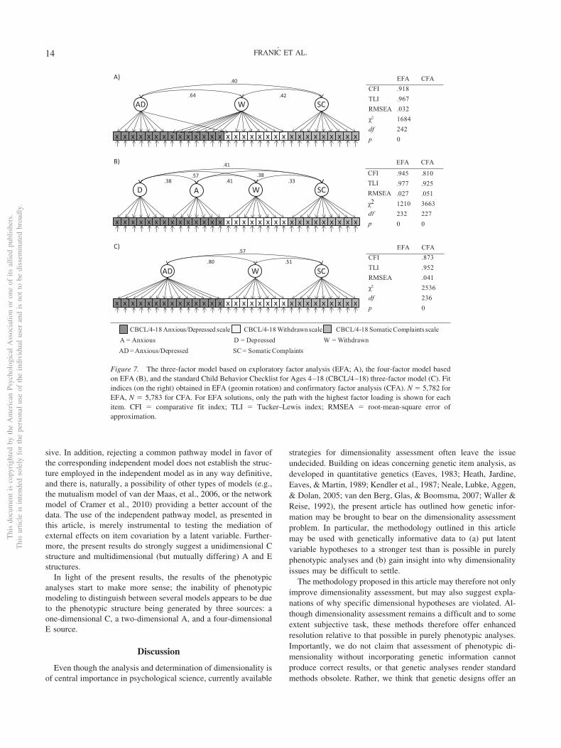
sive. In addition, rejecting a common pathway model in favor ofthe corresponding independent model does not establish the struc-ture employed in the independent model as in any way definitive,and there is, naturally, a possibility of other types of models (e.g.,the mutualism model of van der Maas, et al., 2006, or the networkmodel of Cramer et al., 2010) providing a better account of thedata. The use of the independent pathway model, as presented inthis article, is merely instrumental to testing the mediation ofexternal effects on item covariation by a latent variable. Further-more, the present results do strongly suggest a unidimensional Cstructure and multidimensional (but mutually differing) A and Estructures.
In light of the present results, the results of the phenotypicanalyses start to make more sense; the inability of phenotypicmodeling to distinguish between several models appears to be dueto the phenotypic structure being generated by three sources: aone-dimensional C, a two-dimensional A, and a four-dimensionalE source.
Discussion
Even though the analysis and determination of dimensionality isof central importance in psychological science, currently available
strategies for dimensionality assessment often leave the issueundecided. Building on ideas concerning genetic item analysis, asdeveloped in quantitative genetics (Eaves, 1983; Heath, Jardine,Eaves, & Martin, 1989; Kendler et al., 1987; Neale, Lubke, Aggen,& Dolan, 2005; van den Berg, Glas, & Boomsma, 2007; Waller &Reise, 1992), the present article has outlined how genetic infor-mation may be brought to bear on the dimensionality assessmentproblem. In particular, the methodology outlined in this articlemay be used with genetically informative data to (a) put latentvariable hypotheses to a stronger test than is possible in purelyphenotypic analyses and (b) gain insight into why dimensionalityissues may be difficult to settle.
The methodology proposed in this article may therefore not onlyimprove dimensionality assessment, but may also suggest expla-nations of why specific dimensional hypotheses are violated. Al-though dimensionality assessment remains a difficult and to someextent subjective task, these methods therefore offer enhancedresolution relative to that possible in purely phenotypic analyses.Importantly, we do not claim that assessment of phenotypic di-mensionality without incorporating genetic information cannotproduce correct results, or that genetic analyses render standardmethods obsolete. Rather, we think that genetic designs offer an
EFA CFACFI .945 .810TLI .977 .925RMSEA .027 .051χ2 1210 3663df 232 227p 0 0
A = Anxious D = Depressed W = WithdrawnAD = Anxious/Depressed SC = Somatic Complaints
A) EFA CFACFI .918TLI .967RMSEA .032χ2 1684df 242p 0x x x x x x x x x x x xx x x xx xx x x x x x x x x x x x x
AD W SC.64 .42
.40
CBCL/4-18 Anxious/Depressed scale CBCL/4-18 Withdrawn scale CBCL/4-18 Somatic Complaints scale
x x x x x x x x x x x xx x x xx xx x x x x x x x x x x x x
D W SCA.38 .41 .33
.38
.41
.57
EFA CFACFI .873TLI .952RMSEA .041χ2 2536df 236p 0
x x x x x x x x x x x xx x x xx xx x x x x x x x x x x x x
AD W SC.80 .51
.57
B)
C)
Figure 7. The three-factor model based on exploratory factor analysis (EFA; A), the four-factor model basedon EFA (B), and the standard Child Behavior Checklist for Ages 4–18 (CBCL/4–18) three-factor model (C). Fitindices (on the right) obtained in EFA (geomin rotation) and confirmatory factor analysis (CFA). N � 5,782 forEFA, N � 5,783 for CFA. For EFA solutions, only the path with the highest factor loading is shown for eachitem. CFI � comparative fit index; TLI � Tucker–Lewis index; RMSEA � root-mean-square error ofapproximation.
Thi
sdo
cum
ent
isco
pyri
ghte
dby
the
Am
eric
anPs
ycho
logi
cal
Ass
ocia
tion
oron
eof
itsal
lied
publ
ishe
rs.
Thi
sar
ticle
isin
tend
edso
lely
for
the
pers
onal
use
ofth
ein
divi
dual
user
and
isno
tto
bedi
ssem
inat
edbr
oadl
y.
14 FRANIC ET AL.

underutilized and informative source of data that may help re-searchers to better understand the dimensionality of their con-structs. Practically we envisage a situation in which phenotypicdimensionality research produces varied results, which will inpractice simply result in disagreement concerning dimensionality.For instance, this is the case for cognitive abilities, with respect towhich there are competing models that differ in dimensionality(notwithstanding many decades of research). One solution to thisis to collect larger data sets. However, the present article suggeststo researchers that the greater resolution provided by larger datasets may not provide the answer. We propose that it might beuseful to seek out twin data in order to investigate possible differ-ences in dimensionality of genetic and environment influences onmajor constructs.
As mentioned previously, the logic underlying our approach isessentially the same as that involved in measurement invarianceresearch and MIMIC modeling. Moreover, common and indepen-dent pathway model comparisons have been considered outside thecontext of genetics (see, e.g., Carlson & Mulaik, 1993). However,what makes the analyses presented here different is that unlike instandard MIMIC modeling, the A, C, and E factors determine thevariance of the latent variable completely. Furthermore, the situ-ation in which the common pathway model is rejected is at least asinformative as that in which it is retained, as the informationcontained in genetically informative data sets allows one to exam-ine the exact nature of violations of dimensional assumptions;something that is typically not the case in standard MIMIC mod-eling. In the twin model, one can establish whether or not thecommon pathway model fits and, in case of misfit, can arrive at adetailed account of the cause of misfit, thereby moving the ques-
tion of dimensionality from the phenotypic level to the geneticlevel and the environmental level. This increased resolution (i.e.,the possibility to view the lack of unidimensionality of the ob-served covariation structure as a function of the dimensionalities ofits underlying genetic and environmental structures) is unique tothe twin design and is, in our opinion, a particularly powerfulaspect of the present method.
In our illustrative analyses, the incorporation of genetic infor-mation turned out to be highly informative. In standard phenotypicanalyses, it proved difficult to decide whether a three- or four-dimensional latent structure underlies the data—a situation that isnot uncommon in psychometric investigations into dimensionality,where one often has to decide between solutions that differ sub-stantively but appear to be nearly equivalent statistically. Incorpo-rating genetic information, however, suggested that the reason forthe ambiguity in the data with respect to these structures is thatseveral models are correct, but apply to different sources of itemcovariation: A two-factor model seems to better reflect additivegenetic influences, whereas a four-factor model better reflectsunique environmental influences. Interestingly, common environ-mental influences appear to influence item scores across the board,suggesting that the common part of environmental variation variesalong a single dimension.15
The question of how many dimensions are measured by theInternalizing scales of the CBCL can now be viewed from a newperspective, which may be surprising to the psychometrician: Interms of genetic variance, the items appear to measure two dimen-sions, corresponding to genetic influences distinctly affectingsymptoms of depression, anxiety, and withdrawal, on the onehand, and somatic complaints, on the other. This implies, forinstance, that genes act in a nonspecific way to influence thechance of developing depression-, anxiety-, and withdrawal-related symptomatology. Individual-specific environmental influ-ences distinctly affect symptoms of depression, anxiety, with-drawal, and somatic complaints (thus, individual-specificenvironmental events may be, for example, specifically depresso-genic or specifically anxiogenic), whereas environmental eventsshared by family members appear to have either a positive or anegative effect on the entire range of symptoms. In terms of, forinstance, the anxiety–depression distinction, the present resultssuggest that these two syndromes share the same genetic basis butare distinctly affected by individual-specific environmentalevents—a finding that is in line with prior genetic investigationsinto the dimensionality of anxiety and depression (e.g., Kendler etal., 1987; 1992; Middeldorp et al., 2005).
It should be noted that the current results do not necessarilyreflect upon the utility of the CBCL in the clinical context; we donot doubt its usefulness for diagnostic purposes, especially giventhat the broad structure found in our analyses is in line with thecurrent item allocation of the CBCL. However, in the context ofresearch one should bear in mind that the current scales may notmeasure three distinct sets of genetic, common environmental, andindividual-specific environmental influences but possibly reflect a
15 It is possible that a unidimensional C component partly stems frommethod variance. For instance, variance due to rater bias, if not explicitlymodeled, is absorbed by C (Neale & Cardon, 1992). Given data by multipleraters, it is possible to test for presence of rater bias.
Figure 8. Child Behavior Checklist for Ages 4–18 data: Eigenvalues ofthe �A, �C, and �E matrices (upper panel) and factor loadings obtained inexploratory factor analysis solutions with two A, one C, and four E factors(lower panel). Shading and shapes code for different latent factors. Onlythe highest factor loading for each item is shown.
Thi
sdo
cum
ent
isco
pyri
ghte
dby
the
Am
eric
anPs
ycho
logi
cal
Ass
ocia
tion
oron
eof
itsal
lied
publ
ishe
rs.
Thi
sar
ticle
isin
tend
edso
lely
for
the
pers
onal
use
ofth
ein
divi
dual
user
and
isno
tto
bedi
ssem
inat
edbr
oadl
y.
15CAN GENETICS HELP PSYCHOMETRICS?

more complex underlying structure. Depending on the specificresearch goals, the results of this type of analysis may provide abasis for redefining the current scales to arrive at distinct measuresof each of these sources of influences (e.g., if one’s aim is tomeasure common environmental influences, one may view theitem set as unidimensional and accordingly derive a single sumscore from the data).
Naturally, the results of this type of analyses are relevant notonly to theories of psychopathology; we consider their impli-cations to be much wider. For instance, theories in develop-mental psychology may benefit from investigating the individ-ual differences in the development of behavior as a function ofgenetic and environmental influences, or examining how thevarious dimensions of environmental and genetic influenceschange and develop over time. Also, the results might haveimplications for genetics itself. Specifically, the search forgenes affecting specific behaviors is often based on a compositemeasure of a phenotype, such as a sum score. However, if thesephenotypes are heterogeneous, analogous to the way the CBCLappears heterogeneous, using a total score as a basis for genesearch would appear suboptimal, as the total score itself mightnot accurately reflect the genetic structure underlying the data(van der Sluis, Verhage, Posthuma, & Dolan, 2010). We con-sider this issue to be important, because power to detect theeffects of measured genes is likely to suffer if the phenotypicmeasure is not correctly defined (van der Sluis, et al., 2010).Independent pathway item-level analysis, as described in thisarticle, offers possibilities for redefining the phenotypic scoresin terms of genetic and environmental effects. This may in turnallow for using latent trait estimates derived from a model suchas that in Figure 7 as a basis for gene search.
In addition to these practical benefits of the present method-ology, there are important conceptual considerations that followfrom the ideas presented in this article. For instance, latentvariable models like the factor model can be viewed as incor-porating hypotheses concerning a common-cause structure thatunderlies item covariation (Borsboom, 2008; Borsboom et al.,2003; Haig, 2005a, 2005b). However, the question of whetherlatent variables hypothesized in a given context may be said toexist and have causal relevance is a point of dispute in manyfields; one need only consider the fields of intelligence andpersonality research, where considerable controversy exists re-garding the theoretical status of variables such as the g factorand the five factors of personality. To the extent that suchmodels survive the confrontation with genetic information, asdescribed here, they may be considered more strongly corrob-orated than they could be in analyses of purely phenotypic data.However, if models for genetic and environmental effects havedifferent structures, as was the case for the illustration data inthis article, the common factors found in our phenotypic anal-ysis may in fact be an amalgam of several different genetic andenvironmental models. Clearly, in this case, the ascription ofcausal force to such amalgams is problematic.
In conclusion, we expect that the methodology proposed inthis article may bear considerable fruit in disentangling dimen-sionality issues in the research areas where they have generatedcontroversy, and shed light on the theoretical status of impor-tant hypothesized latent variables in intelligence, psychopathol-ogy, and personality research. The time is ripe for investiga-tions along these lines. In the past decades, behavior geneticsresearchers have constructed large and well-archived twin andfamily registries that are perfectly suited for analyses such as
Figure 9. The 2A 1C 4E independent pathway model for the Child Behavior Checklist for Ages 4–18
(CBCL/4–18) Internalizing scale. Item residuals are not depicted but are estimated in the model. �� denotes theaverage factor loading associated with a factor. A � Anxious; D � Depressed; W � Withdrawn; SC � SomaticComplaints.
Thi
sdo
cum
ent
isco
pyri
ghte
dby
the
Am
eric
anPs
ycho
logi
cal
Ass
ocia
tion
oron
eof
itsal
lied
publ
ishe
rs.
Thi
sar
ticle
isin
tend
edso
lely
for
the
pers
onal
use
ofth
ein
divi
dual
user
and
isno
tto
bedi
ssem
inat
edbr
oadl
y.
16 FRANIC ET AL.

those reported here (e.g., a 1998 review lists 16 twin registriesin Europe alone; Boomsma, 1998; Busjahn, 2002). The data setscontained in those registries are typically obtainable via proto-cols for collaborative projects, and in some cases even publi-cally available (e.g., Add Health; see Harris, Halpern, Smolen,& Haberstick, 2006). In addition, the development of psycho-metric software as well as the current speed of computers hasled to a situation where the required statistical analyses havebecome feasible. In our view, this opens up a wealth of possi-bilities for refining and extending psychometric investigationsbeyond the analysis of purely phenotypic covariation.
References
Achenbach, T. M. (1966). Classification of children’s psychiatric symp-toms: A factor-analytic study. Psychological Monographs: General andApplied, 80(7, Whole No. 615). doi:10.1037/h0093906
Achenbach, T. M. (1991). Manual for the Child Behavior Checklist/4-18and 1991 profile. Burlington: University of Vermont, Department ofPsychiatry.
Ackerman, P. L., Beier, M. E., & Boyle, M. O. (2005). Working memoryand intelligence: The same or different constructs? Psychological Bul-letin, 131(1), 30–60. doi:10.1037/0033-2909.131.1.30
American Psychiatric Association. (1994). Diagnostic and statistical man-ual of mental disorders (4th ed.). Washington, DC: Author.
Angold, A., Costello, E. J., & Erkanli, A. (1999). Comorbidity. Journal ofChild Psychology and Psychiatry, 40(1), 57–87. doi:10.1111/1469-7610.00424
Bartels, M., Boomsma, D. I., Hudziak, J. J., van Beijsterveldt, T. C. E. M.,& van den Oord, E. J. C. G. (2007). Twins and the study of rater(dis)agreement. Psychological Methods, 12(4), 451466. doi:10.1037/1082-989X.12.4.451
Bartels, M., van Beijsterveldt, C. E. M., Derks, E. M., Stroet, T. M.,Polderman, T. J. C., Hudziak, J. J.,& Boomsma, D. I. (2007). YoungNetherlands Twin Register (Y-NTR): A longitudinal multiple informantstudy of problem behavior. Twin Research and Human Genetics, 10(1),3–11. doi:10.1375/twin.10.1.3
Bollen, K. A. (1989). Structural equations with latent variables. NewYork, NY: Wiley.
Boomsma, D. I. (1998). Twin registers in Europe: An overview. TwinResearch, 1(1), 34–51.
Boomsma, D., Busjahn, A., & Peltonen, L. (2002). Classical twin studiesand beyond. Nature Reviews Genetics, 3(11), 872–882. doi:10.1038/nrg932
Boomsma, D. I., de Geus, E. J. C., Vink, J. M., Stubbe, J. H., Distel, M. A.,Hottenga, J.-J., . . . Willemsen, G. (2006). Netherlands Twin Register:From twins to twin families. Twin Research and Human Genetics, 9(6),849–857. doi:10.1375/twin.9.6.849
Boomsma, D. I., & Molenaar, P. C. M. (1986). Using LISREL to analyzegenetic and environmental covariance structure. Behavior Genetics,16(2), 237–250. doi:10.1007/BF01070799
Boomsma, D. I., & Molenaar, P. C. M. (1987). The genetic-analysis ofrepeated measures. 1. Simplex models. Behavior Genetics, 17(2), 111–123. doi:10.1007/BF01065991
Borsboom, D. (2008). Psychometric perspectives on diagnostic systems.Journal of Clinical Psychology, 64(9), 1089–1108. doi:10.1002/jclp.20503
Borsboom, D., Mellenbergh, G. J., & van Heerden, J. (2003). The theo-retical status of latent variables. Psychological Review, 110(2), 203–219.doi:10.1037/0033-295X.110.2.203
Brady, E. U., & Kendall, P. C. (1992). Comorbidity of anxiety anddepression in children and adolescents. Psychological Bulletin, 111(2),244–255. doi:10.1037/0033-2909.111.2.244
Busjahn, A. (Ed.). (2002). Twin registers as a global resource for geneticresearch [Special Issue]. Twin Research, 5(5).
Carlson, M., & Mulaik, S. A. (1993). Trait ratings from descriptions ofbehavior as mediated by components of meaning. Multivariate Behav-ioral Research, 28(1), 111–159. doi:10.1207/s15327906mbr2801_7
Carroll, J. B. (2003). The higher-stratum structure of cognitive abilities:Current evidence supports g and about ten broad factors. In H. Nyborg(Ed.), The scientific study of general intelligence: Tribute to Arthur R.Jensen (pp. 5–21). New York, NY: Pergamon. doi:10.1016/B978-008043793-4/50036-2
Cattell, R. B. (1941). Some theoretical issues in adult intelligence testing[Abstract of poster presented at the annual meeting of the AmericanPsychological Association]. Psychological Bulletin, 38(7), 592.
Cherny, S. S. (2008). Variance components and related methods for map-ping quantitative trait loci. Sociological Methods & Research, 37(2),227–250. doi:10.1177/0049124108324524
Clark, L. A. (1989). The anxiety and depressive disorders: Descriptivepsychopathology and differential diagnosis. In P. C. Kendall & D.Watson (Eds.), Anxiety and depression: Distinctive and overlappingfeatures (pp. 83–129). New York, NY: Academic Press.
Clark, L. A., & Watson, D. (1991). Tripartite model of anxiety anddepression: Psychometric evidence and taxonomic implications. Journalof Abnormal Psychology, 100(3), 316–336. doi:10.1037/0021-843X.100.3.316
Costa, P. T., Jr., & McCrae, R. R. (1985). The NEO Personality Inventorymanual. Odessa, FL: Psychological Assessment Resources.
Cramer, A. O. J., Waldorp, L. J., van der Maas, H. L. J., & Borsboom, D.(2010). Comorbidity: A network perspective. Behavioral and BrainSciences, 33(2–3), 137–150. doi:10.1017/S0140525X09991567
Cronbach, L. J., & Meehl, P. E. (1955). Construct validity in psychologicaltests. Psychological Bulletin, 52(4), 281–302. doi:10.1037/h0040957
Derks, E. M., Dolan, C. V., & Boomsma, D. I. (2006). A test of the equalenvironment assumption (EEA) in multivariate twin studies. Twin Re-search and Human Genetics, 9(3), 403–411. doi:10.1375/twin.9.3.403
Dolan, C. V. (1992). Biometric decomposition of phenotypic means inhuman samples (Unpublished doctoral dissertation). University of Am-sterdam, Amsterdam, the Netherlands.
Eaves, L. J. (1983). Errors of inference in the detection of major geneeffects on psychological test scores. American Journal of Human Ge-netics, 35(6), 1179–1189.
Eaves, L. J., Long, J., & Heath, A. C. (1986). A theory of developmentalchange in quantitative phenotypes applied to cognitive development.Behavior Genetics, 16(1), 143–162. doi:10.1007/BF01065484
Fabrigar, L. R., Wegener, D. T., MacCallum, R. C., & Strahan, E. J.(1999). Evaluating the use of exploratory factor analysis in psycholog-ical research. Psychological Methods, 4(3), 272–299. doi:10.1037/1082-989X.4.3.272
Falconer, D. S., & Mackay, T. F. C. (1996). Introduction to quantitativegenetics (4th ed.). Harlow, England: Longmans Green.
Flora, D. B., & Curran, P. J. (2004). An empirical evaluation of alternativemethods of estimation for confirmatory factor analysis with ordinal data.Psychological Methods, 9(4), 466–491. doi:10.1037/1082-989X.9.4.466
Franic, S., Dolan, C. V., Borsboom, D., & Boomsma, D. I. (2012).Structural equation modeling in genetics. In R. H. Hoyle (Ed.), Hand-book of structural equation modeling (pp. 617–635). New York, NY:Guilford Press.
Goldberg, L. R. (1990). An alternative “description of personality”: TheBig-Five factor structure. Journal of Personality and Social Psychology,59(6), 1216–1229. doi:10.1037/0022-3514.59.6.1216
Gorsuch, R. L. (1983). Factor analysis (2nd ed.). Hillsdale, NJ: Erlbaum.Haig, B. D. (2005a). An abductive theory of scientific method. Psycho-
logical Methods, 10(4), 371–388. doi:10.1037/1082-989X.10.4.371
Thi
sdo
cum
ent
isco
pyri
ghte
dby
the
Am
eric
anPs
ycho
logi
cal
Ass
ocia
tion
oron
eof
itsal
lied
publ
ishe
rs.
Thi
sar
ticle
isin
tend
edso
lely
for
the
pers
onal
use
ofth
ein
divi
dual
user
and
isno
tto
bedi
ssem
inat
edbr
oadl
y.
17CAN GENETICS HELP PSYCHOMETRICS?

Haig, B. D. (2005b). Exploratory factor analysis, theory generation, andscientific method. Multivariate Behavioral Research, 40(3), 303–329.doi:10.1207/s15327906mbr4003_2
Harris, K. M., Halpern, C. T., Smolen, A., & Haberstick, B. C. (2006). TheNational Longitudinal Study of Adolescent Health (Add Health) twindata. Twin Research and Human Genetics, 9(6), 988–997. doi:10.1375/twin.9.6.988
Heath, A. C., Jardine, R., Eaves, L. J., & Martin, N. G. (1989). The geneticstructure of personality—II. Genetic item analysis of the EPQ. Person-ality and Individual Differences, 10(6), 615–624. doi:10.1016/0191-8869(89)90221-3
Henson, R. K., & Roberts, J. K. (2006). Use of exploratory factor analysisin published research: Common errors and some comment on improvedpractice. Educational and Psychological Measurement, 66(3), 393–416.doi:10.1177/0013164405282485
Horn, J. L. (1965). Fluid and crystallized intelligence: A factor analyticand developmental study of the structure among primary mental abilities(Unpublished doctoral dissertation). University of Illinois, Champaign.
Jöreskog, K. G. (1993). Testing structural equation models. In K. A. Bollen& S. J. Long (Eds.), Testing structural equation models (pp. 294–316).Newbury Park, CA: Sage.
Jöreskog, K., & Goldberger, S. (1975). Estimation of a model with multipleindicators and multiple causes of a single latent variable. Journal ofAmerican Statistical Association, 70, 631–639.
Kendler, K. S., Heath, A. C., Martin, N. G., & Eaves, L. J. (1987).Symptoms of anxiety and symptoms of depression: Same genes, differ-ent environments. Archives of General Psychiatry, 44(5), 451–457.doi:10.1001/archpsyc.1987.01800170073010
Kendler, K. S., Neale, M. C., Kessler, R. C., Heath, A. C., & Eaves, L. J.(1992). Major depression and generalized anxiety disorder: Same genes,(partly) different environments. Archives of General Psychiatry, 49(9),716–722. doi:10.1001/archpsyc.1992.01820090044008
Kline, R. B. (2005). Principles and practice of structural equation mod-eling (2nd ed.). New York, NY: Guilford Press.
Lawley, D. N., & Maxwell, A. E. (1971). Factor analysis as a statisticalmethod (2nd ed.). London, England: Butterworths.
Lilienfeld, S. O., Waldman, I. D., & Israel, A. C. (1994). A criticalexamination of the use of the term and concept of comorbidity inpsychopathology research. Clinical Psychology: Science and Practice,1(1), 71–83. doi:10.1111/j.1468-2850.1994.tb00007.x
Lykken, D. T., McGue, M., Bouchard, T. J., & Tellegen, A. (1990). Doescontact lead to similarity or similarity to contact. Behavior Genetics,20(5), 547–561. doi:10.1007/BF01065871
Lykken, D. T., McGue, M., & Tellegen, A. (1987). Recruitment bias intwin research: The rule of two-thirds reconsidered. Behavior Genetics,17(4), 343–362. doi:10.1007/BF01068136
Martin, N., Boomsma, D., & Machin, G. (1997). A twin-pronged attack oncomplex traits. Nature Genetics, 17(4), 387–392. doi:10.1038/ng1297-387
Martin, N. G., & Eaves, L. J. (1977). Genetic analysis of covariancestructure. Heredity, 38(1), 79–95. doi:10.1038/hdy.1977.9
Martin, N. G., & Wilson, S. R. (1982). Bias in the estimation of heritabilityfrom truncated samples of twins. Behavior Genetics, 12(4), 467–472.doi:10.1007/BF01065638
Matzke, D., Dolan, C. V., & Molenaar, D. (2010). The issue of power inthe identification of “g” with lower-order factors. Intelligence, 38(3),336–344. doi:10.1016/j.intell.2010.02.001
McArdle, J. J., & Goldsmith, H. H. (1990). Alternative common factormodels for multivariate biometric analyses. Behavior Genetics, 20(5),569–608. doi:10.1007/BF01065873
McCrae, R. R., & Costa, P. T., Jr. (1999). A five-factor theory of person-ality. In L. A. Pervin & O. P. John (Eds.), Handbook of personality:Theory and research (2nd ed., pp. 139–153). New York, NY: GuilfordPress.
McCrae, R. R., & John, O. P. (1992). An introduction to the five-factormodel and its applications. Journal of Personality, 60(2), 175–215.doi:10.1111/j.1467-6494.1992.tb00970.x
Medland, S. E., & Neale, M. C. (2010). An integrated phenomic approachto multivariate allelic association. European Journal of Human Genet-ics, 18(2), 233–239. doi:10.1038/ejhg.2009.133
Mellenbergh, G. J. (1989). Item bias and item response theory. Interna-tional Journal of Educational Research, 13(2), 127–143. doi:10.1016/0883-0355(89)90002-5
Meredith, W. (1993). Measurement invariance, factor analysis and factorialinvariance. Psychometrika, 58(4), 525–543. doi:10.1007/BF02294825
Middeldorp, C. M., Cath, D. C., Van Dyck, R., & Boomsma, D. I.(2005). The co-morbidity of anxiety and depression in the perspec-tive of genetic epidemiology. A review of twin and family studies.Psychological Medicine, 35(5), 611– 624. doi:10.1017/S003329170400412X
Mulaik, S. A. (1987). A brief history of the philosophical foundations ofexploratory factor analysis. Multivariate Behavioral Research, 22(3),267–305. doi:10.1207/s15327906mbr2203_3
Muthén, L. K., & Muthén, B. O. (2007a). Mplus (Version 5.1) [Computersoftware]. Los Angeles, CA: Muthén & Muthén.
Muthén, L. K., & Muthén, B. O. (2007b). Mplus user’s guide (5th ed.). LosAngeles, CA Muthén & Muthén.
Neale, M. C. (2000). MxGui (Version 1.7.03) [Computer software]. Rich-mond: Virginia Commonwealth University. Retrieved from http://www.vcu.edu/mx/
Neale, M. C., & Cardon, L. (1992). Methodology for genetic studies oftwins and families. Dordrecht, the Netherlands: Kluwer Academic. doi:10.1007/978-94-015-8018-2
Neale, M. C., Eaves, L. J., Kendler, K. S., & Hewitt, J. K. (1989). Biasin correlations from selected samples of relatives: The effects of softselection. Behavior Genetics, 19(2), 163–169. doi:10.1007/BF01065901
Neale, M. C., Lubke, G., Aggen, S. H., & Dolan, C. V. (2005). Problemswith using sum scores for estimating variance components: Contamina-tion and measurement noninvariance. Twin Research and Human Ge-netics, 8(6), 553–568. doi:10.1375/twin.8.6.553
Pearl, J. (2000). Causality: Models, reasoning, and inference. New York,NY: Oxford University Press.
Plomin, R., Defries, J. C., McClearn, G. E., & McGuffin, P. (2008).Behavioral genetics (5th ed.). New York, NY: Freeman.
Purcell, S. (2002). Variance components models for gene–environmentinteraction in twin analysis. Twin Research, 5(6), 554–571.
R Development Core Team. (2009). R: A language and environment forstatistical computing (Version 2.15.2) [Computer software]. Vienna,Austria: R Foundation for Statistical Computing. Retrieved from http://cran.r-project.org/bin/windows/base/
Rebollo, I., de Moor, M. H. M., Dolan, C. V., & Boomsma, D. I. (2006).Phenotypic factor analysis of family data: Correction of the bias due todependency. Twin Research and Human Genetics, 9(3), 367–376. doi:10.1375/twin.9.3.367
Rummel, R. J. (1970). Applied factor analysis. Evanston, IL: NorthwesternUniversity Press.
Satorra, A., & Bentler, P. M. (2001). A scaled difference chi-square teststatistic for moment structure analysis. Psychometrika, 66(4), 507–514.doi:10.1007/BF02296192
Stoolmiller, M. (1999). Implications of the restricted range of familyenvironments for estimates of heritability and nonshared environment inbehavior-genetic adoption studies. Psychological Bulletin, 125(4), 392–409. doi:10.1037/0033-2909.125.4.392
van den Berg, S. M., Glas, C. A. W., & Boomsma, D. I. (2007). Variancedecomposition using an IRT measurement model. Behavior Genetics,37(4), 604–616. doi:10.1007/s10519-007-9156-1
Thi
sdo
cum
ent
isco
pyri
ghte
dby
the
Am
eric
anPs
ycho
logi
cal
Ass
ocia
tion
oron
eof
itsal
lied
publ
ishe
rs.
Thi
sar
ticle
isin
tend
edso
lely
for
the
pers
onal
use
ofth
ein
divi
dual
user
and
isno
tto
bedi
ssem
inat
edbr
oadl
y.
18 FRANIC ET AL.

van der Maas, H. L. J., Dolan, C. V., Grasman, R. P. P. P., Wicherts, J. M.,Huizenga, H. M., & Raijmakers, M. E. J. (2006). A dynamical model of generalintelligence: The positive manifold of intelligence by mutualism. PsychologicalReview, 113(4), 842–861. doi:10.1037/0033-295X.113.4.842
van der Sluis, S., Dolan, C. V., Neale, M. C., & Posthuma, D. (2008). Powercalculations using exact data simulation: A useful tool for genetic study designs.Behavior Genetics, 38(2), 202–211. doi:10.1007/s10519-007-9184-x
van der Sluis, S., Verhage, M., Posthuma, D., & Dolan, C. V. (2010).Phenotypic complexity, measurement bias, and poor phenotypic resolu-tion contribute to the missing heritability problem in genetic associationstudies. PLoS ONE, 5(11), e13929. doi:10.1371/journal.pone.0013929
van Dongen, J., Draisma, H. H. M., Martin, N. G., & Boomsma, D. I.(2012). The continuing value of twin studies in the omics era. NatureReviews Genetics, 13(9), 640–653. doi:10.1038/nrg3243
Verhulst, F. C., Van der Ende, J., & Koot, H. M. (1996). Handleidingvoor de CBCL/4 –18 (CBCL/4 –18 manual]. Rotterdam, the Nether-lands: Erasmus University, Academic Medical Centre Rotterdam/Sophia Children’s Hospital, Department of Child Psychiatry.
Waller, N. G., & Reise, S. P. (1992). Genetic and environmental influenceson item response pattern scalability. Behavior Genetics, 22(2), 135–152.doi:10.1007/BF01066993
Wirth, R. J., & Edwards, M. C. (2007). Item factor analysis: Currentapproaches and future directions. Psychological Methods, 12(1), 58–79.doi:10.1037/1082-989X.12.1.58
Yung, Y. F., Thissen, D., & McLeod, L. D. (1999). On the relationshipbetween the higher-order factor model and the hierarchicalfactor model. Psychometrika, 64(2), 113–128. doi:10.1007/BF02294531
Zwick, W. R., & Velicer, W. F. (1982). Factors influencing four rulesfor determining the number of components to retain. MultivariateBehavioral Research, 17(2), 253–269. doi:10.1207/s15327906mbr1702_5
Zwick, W. R., & Velicer, W. F. (1986). Comparison of five rules fordetermining the number of components to retain. Psychological Bul-letin, 99(3), 432– 442. doi:10.1037/0033-2909.99.3.432
Appendix A
Model for the Residuals in the Simulation Study
The residuals of items in the model may also be subjected toa decomposition into genetic and environmental components.The model for the residuals was not detailed in the main text,where it was merely stated that the parameter values for theresidual matrices were obtained by subtraction, for example,�cp � �ip � I � diag[�(�A � �C � ��)�t]. However, theresiduals in the current simulations conform to an ACE model,and could alternatively be simulated by specifying the expectedresidual covariance matrix as a function of residual ACE pa-rameters:
��11 �12
�21 �22��
��AA�At � �CC�C
t � �EE�Et rA�AA�A
t � �CC�Ct
rA�AA�At � �CC�C
t �AA�At � �CC�C
t � �EE�Et �,
where �11(�22) is the 12 � 12 matrix of residual item vari-ances of Twin 1 (Twin 2); �12(�21) is the 12 � 12 Twin 1 �Twin 2 residual covariance matrix; �A, �C, and �E are thediagonal matrices containing the factor loadings of the items onthe residual (item-specific) A, C, and E factors; A, C, andE are the covariance matrices of the residual A, C, and Efactors; and rA is the additive genetic twin correlation (1 formonozygotic [MZ] twins, .5 for dizygotic [DZ] twins). Notethat because the residual covariance matrices were simulated tobe equal across all the models above (e.g., �ip � �cp, �ip21mz �
�cp21mz, and �ip21dz � �cp21dz), in the expression above wedispose of the “cp” and “ip” notation. Figure A1 depicts theACE model for the residuals.
The residual parameter values were equal across the four mod-els:
A � C � E � diag(1, 1, 1, 1, 1, 1, 1, 1, 1, 1, 1, 1),
�A � diag(�.450, �.425, �.400, �.375, �.350, �.325,�.300, �.275, �.250, �.225, �.200, �.175),
�C � diag(�.270, �.255, �.240, �.225, �.210, �.195,�.180, �.165, �.150, �.135, �.120, �.105),
�E � diag(�.18, �.17, �.16, �.15, �.14, �.13, �.12,�.11, �.10, �.09, �.08, �.07).
Coming back to Expression 1 in the main text:
��11 �12
�21 �22�� ��A � �C � �E rA�A � �C
rA�A � �C �A � �C � �E�,
we may now note that �A is a function of both common andresidual additive genetic influences, that is, �A � ��A�t ��AA�A
t (or �A � �A�A�At � �AA�A
t in an independentpathway model). Similarly, �C � ��C�t � �CC�C
t, etc.
(Appendices continue)
Thi
sdo
cum
ent
isco
pyri
ghte
dby
the
Am
eric
anPs
ycho
logi
cal
Ass
ocia
tion
oron
eof
itsal
lied
publ
ishe
rs.
Thi
sar
ticle
isin
tend
edso
lely
for
the
pers
onal
use
ofth
ein
divi
dual
user
and
isno
tto
bedi
ssem
inat
edbr
oadl
y.
19CAN GENETICS HELP PSYCHOMETRICS?
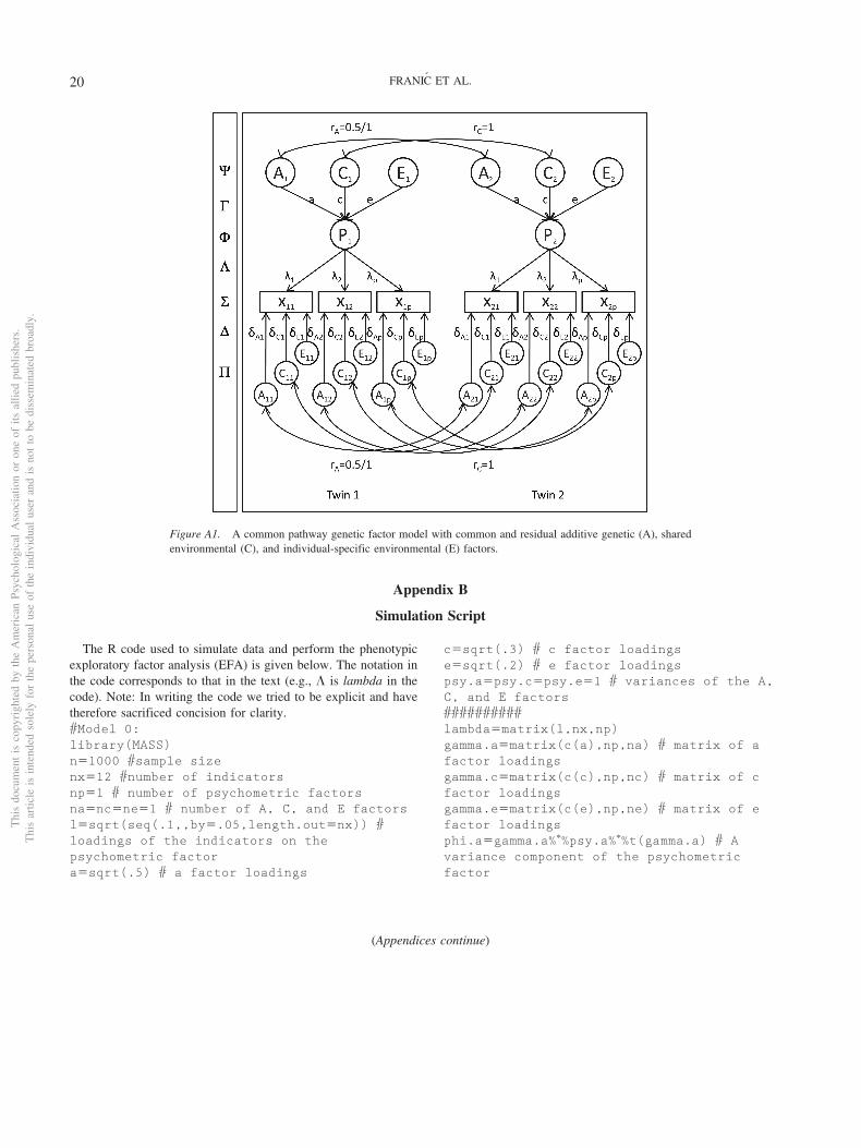
Appendix B
Simulation Script
The R code used to simulate data and perform the phenotypicexploratory factor analysis (EFA) is given below. The notation inthe code corresponds to that in the text (e.g., � is lambda in thecode). Note: In writing the code we tried to be explicit and havetherefore sacrificed concision for clarity.#Model 0:library(MASS)n�1000 #sample sizenx�12 #number of indicatorsnp�1 # number of psychometric factorsna�nc�ne�1 # number of A, C, and E factorsl�sqrt(seq(.1,,by�.05,length.out�nx)) #loadings of the indicators on thepsychometric factora�sqrt(.5) # a factor loadings
c�sqrt(.3) # c factor loadingse�sqrt(.2) # e factor loadingspsy.a�psy.c�psy.e�1 # variances of the A,C, and E factors##########lambda�matrix(l,nx,np)gamma.a�matrix(c(a),np,na) # matrix of afactor loadingsgamma.c�matrix(c(c),np,nc) # matrix of cfactor loadingsgamma.e�matrix(c(e),np,ne) # matrix of efactor loadingsphi.a�gamma.a%�%psy.a%�%t(gamma.a) # Avariance component of the psychometricfactor
(Appendices continue)
Figure A1. A common pathway genetic factor model with common and residual additive genetic (A), sharedenvironmental (C), and individual-specific environmental (E) factors.
Thi
sdo
cum
ent
isco
pyri
ghte
dby
the
Am
eric
anPs
ycho
logi
cal
Ass
ocia
tion
oron
eof
itsal
lied
publ
ishe
rs.
Thi
sar
ticle
isin
tend
edso
lely
for
the
pers
onal
use
ofth
ein
divi
dual
user
and
isno
tto
bedi
ssem
inat
edbr
oadl
y.
20 FRANIC ET AL.
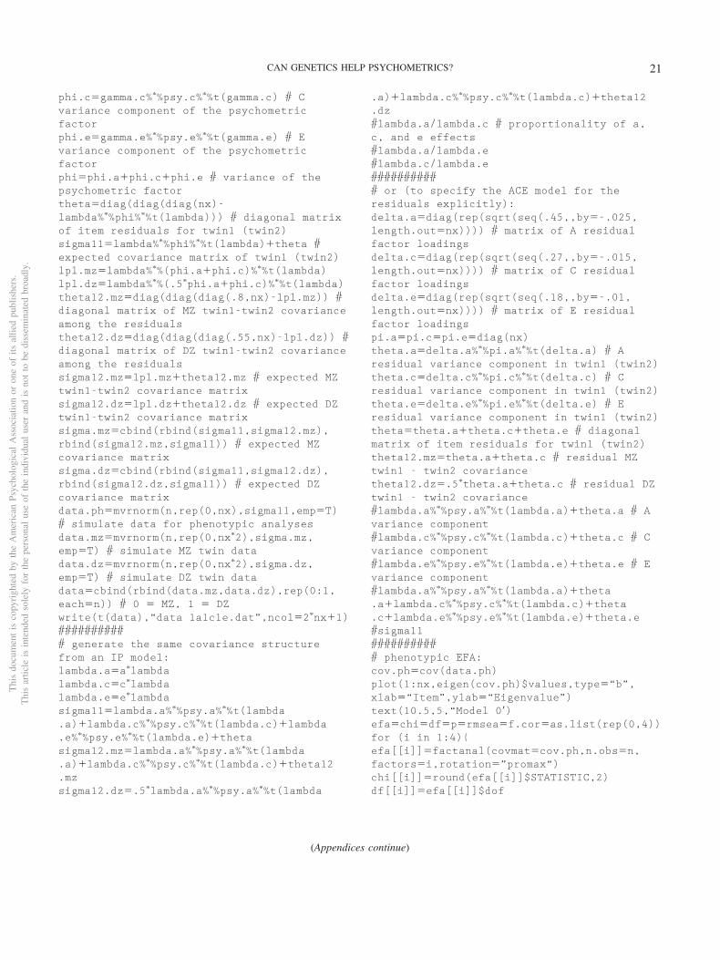
phi.c�gamma.c%�%psy.c%�%t(gamma.c) # Cvariance component of the psychometricfactorphi.e�gamma.e%�%psy.e%�%t(gamma.e) # Evariance component of the psychometricfactorphi�phi.a�phi.c�phi.e # variance of thepsychometric factortheta�diag(diag(diag(nx)-lambda%�%phi%�%t(lambda))) # diagonal matrixof item residuals for twin1 (twin2)sigma11�lambda%�%phi%�%t(lambda)�theta #expected covariance matrix of twin1 (twin2)lpl.mz�lambda%�%(phi.a�phi.c)%�%t(lambda)lpl.dz�lambda%�%(.5�phi.a�phi.c)%�%t(lambda)theta12.mz�diag(diag(diag(.8,nx)-lpl.mz)) #diagonal matrix of MZ twin1-twin2 covarianceamong the residualstheta12.dz�diag(diag(diag(.55,nx)-lpl.dz)) #diagonal matrix of DZ twin1-twin2 covarianceamong the residualssigma12.mz�lpl.mz�theta12.mz # expected MZtwin1-twin2 covariance matrixsigma12.dz�lpl.dz�theta12.dz # expected DZtwin1-twin2 covariance matrixsigma.mz�cbind(rbind(sigma11,sigma12.mz),rbind(sigma12.mz,sigma11)) # expected MZcovariance matrixsigma.dz�cbind(rbind(sigma11,sigma12.dz),rbind(sigma12.dz,sigma11)) # expected DZcovariance matrixdata.ph�mvrnorm(n,rep(0,nx),sigma11,emp�T)# simulate data for phenotypic analysesdata.mz�mvrnorm(n,rep(0,nx�2),sigma.mz,emp�T) # simulate MZ twin datadata.dz�mvrnorm(n,rep(0,nx�2),sigma.dz,emp�T) # simulate DZ twin datadata�cbind(rbind(data.mz,data.dz),rep(0:1,each�n)) # 0 � MZ, 1 � DZwrite(t(data),“data 1a1c1e.dat”,ncol�2�nx�1)########### generate the same covariance structurefrom an IP model:lambda.a�a�lambdalambda.c�c�lambdalambda.e�e�lambdasigma11�lambda.a%�%psy.a%�%t(lambda.a)�lambda.c%�%psy.c%�%t(lambda.c)�lambda.e%�%psy.e%�%t(lambda.e)�thetasigma12.mz�lambda.a%�%psy.a%�%t(lambda.a)�lambda.c%�%psy.c%�%t(lambda.c)�theta12.mzsigma12.dz�.5�lambda.a%�%psy.a%�%t(lambda
.a)�lambda.c%�%psy.c%�%t(lambda.c)�theta12
.dz#lambda.a/lambda.c # proportionality of a,c, and e effects#lambda.a/lambda.e#lambda.c/lambda.e########### or (to specify the ACE model for theresiduals explicitly):delta.a�diag(rep(sqrt(seq(.45,,by�-.025,length.out�nx)))) # matrix of A residualfactor loadingsdelta.c�diag(rep(sqrt(seq(.27,,by�-.015,length.out�nx)))) # matrix of C residualfactor loadingsdelta.e�diag(rep(sqrt(seq(.18,,by�-.01,length.out�nx)))) # matrix of E residualfactor loadingspi.a�pi.c�pi.e�diag(nx)theta.a�delta.a%�%pi.a%�%t(delta.a) # Aresidual variance component in twin1 (twin2)theta.c�delta.c%�%pi.c%�%t(delta.c) # Cresidual variance component in twin1 (twin2)theta.e�delta.e%�%pi.e%�%t(delta.e) # Eresidual variance component in twin1 (twin2)theta�theta.a�theta.c�theta.e # diagonalmatrix of item residuals for twin1 (twin2)theta12.mz�theta.a�theta.c # residual MZtwin1 - twin2 covariancetheta12.dz�.5�theta.a�theta.c # residual DZtwin1 - twin2 covariance#lambda.a%�%psy.a%�%t(lambda.a)�theta.a # Avariance component#lambda.c%�%psy.c%�%t(lambda.c)�theta.c # Cvariance component#lambda.e%�%psy.e%�%t(lambda.e)�theta.e # Evariance component#lambda.a%�%psy.a%�%t(lambda.a)�theta.a�lambda.c%�%psy.c%�%t(lambda.c)�theta.c�lambda.e%�%psy.e%�%t(lambda.e)�theta.e#sigma11########### phenotypic EFA:cov.ph�cov(data.ph)plot(1:nx,eigen(cov.ph)$values,type�“b”,xlab�“Item”,ylab�“Eigenvalue”)text(10.5,5,“Model 0=)efa�chi�df�p�rmsea�f.cor�as.list(rep(0,4))for (i in 1:4){efa[[i]]�factanal(covmat�cov.ph,n.obs�n,factors�i,rotation�”promax“)chi[[i]]�round(efa[[i]]$STATISTIC,2)df[[i]]�efa[[i]]$dof
(Appendices continue)
Thi
sdo
cum
ent
isco
pyri
ghte
dby
the
Am
eric
anPs
ycho
logi
cal
Ass
ocia
tion
oron
eof
itsal
lied
publ
ishe
rs.
Thi
sar
ticle
isin
tend
edso
lely
for
the
pers
onal
use
ofth
ein
divi
dual
user
and
isno
tto
bedi
ssem
inat
edbr
oadl
y.
21CAN GENETICS HELP PSYCHOMETRICS?

p[[i]]�round(efa[[i]]$PVAL,2)if(chi[[i]]-df[[i]]�0) {rmsea[[i]]�(sqrt(chi[[i]]-df[[i]]))/n/df[[i]]}if(i � 1) {rm�promax(unclass(efa[[i]]$loadings))$rotmatf.cor[[i]]�solve(rm%�%t(rm))}}res�cbind(chi,df,p,rmsea)dimnames(res)[[1]]�paste(1:4,”factors’,sep�”)res###########Model 1:na_m2�2lambda.a_m2�matrix(c(a�lambda[1:6,],rep(0,nx),a�lambda[7:12,]),nx,na_m2)psy.a_m2�diag(na_m2)sigma11_m2�lambda.a_m2%�%psy.a_m2%�%t(lambda.a_m2)�lambda.c%�%psy.c%�%t(lambda.c)�lambda.e%�%psy.e%�%t(lambda.e)�thetasigma12.mz_m2�lambda.a_m2%�%psy.a_m2%�%t(lambda.a_m2)�lambda.c%�%psy.c%�%t(lambda.c)�theta12.mzsigma12.dz_m2�.5�lambda.a_m2%�%psy.a_m2%�%t(lambda.a_m2)�lambda.c%�%psy.c%�%t(lambda.c)�theta12.dzsigma.mz_m2�cbind(rbind(sigma11_m2,sigma12.mz_m2),rbind(sigma12.mz_m2,sigma11_m2)) #expected MZ covariance matrixsigma.dz_m2�cbind(rbind(sigma11_m2,sigma12.dz_m2),rbind(sigma12.dz_m2,sigma11_m2)) #expected DZ covariance matrixdata.ph�mvrnorm(n,rep(0,nx),sigma11_m2,emp�T) # simulate data for phenotypicanalysesdata.mz�mvrnorm(n,rep(0,nx�2),sigma.mz_m2,emp�T) # simulate MZ twin datadata.dz�mvrnorm(n,rep(0,nx�2),sigma.dz_m2,emp�T) # simulate DZ twin datadata�cbind(rbind(data.mz,data.dz),rep(0:1,each�n)) # 0 � MZ, 1 � DZwrite(t(data),“data 2a1c1e.dat”,ncol�2�nx�1)###########Model 2:ne_m3�2lambda.e_m3�matrix(c(e�lambda[1:3],rep(0,6),e�lambda[10:12],rep(0,3),e�lambda[4:9],rep(0,3)),nx,ne_m3)psy.e_m3�diag(ne_m3)sigma11_m3�lambda.a_m2%�%psy.a_m2%�%t(lambda.a_m2)�lambda.c%�%psy.c%�%t(lambda.c)�lambda.e_m3%�%psy.e_m3%�%t(lambda.e_m3)�thetasigma12.mz_m3�lambda.a_m2%�%psy
.a_m2%�%t(lambda.a_m2)�lambda.c%�%psy
.c%�%t(lambda.c)�theta12.mzsigma12.dz_m3�.5�lambda.a_m2%�%psy.a_m2%�%t(lambda.a_m2)�lambda.c%�%psy.c%�%t(lambda.c)�theta12.dzsigma.mz_m3�cbind(rbind(sigma11_m3,sigma12.mz_m3),rbind(sigma12.mz_m3,sigma11_m3)) #expected MZ covariance matrixsigma.dz_m3�cbind(rbind(sigma11_m3,sigma12.dz_m3),rbind(sigma12.dz_m3,sigma11_m3)) #expected DZ covariance matrixdata.ph�mvrnorm(n,rep(0,nx),sigma11_m3,emp�T) # simulate data for phenotypicanalysesdata.mz�mvrnorm(n,rep(0,nx�2),sigma.mz_m3,emp�T) # simulate MZ twin datadata.dz�mvrnorm(n,rep(0,nx�2),sigma.dz_m3,emp�T) # simulate DZ twin datadata�cbind(rbind(data.mz,data.dz),rep(0:1,each�n)) # 0 � MZ, 1 � DZ#write(t(data),“data 2a1c2e.dat”,ncol�2�nx�1)###########Model 3:nc_m4�3lambda.c_m4a�t(matrix(c(1,0,0,0,1,0,0,0,1,1,0,0,0,1,0,0,0,1,1,0,0,0,1,0,0,0,1,1,0,0,0,1,0,0,0,1),nx,nc_m4,byrow�T))lambda.c_m4a[lambda.c_m4a��1]�c�lambdalambda.c_m4�t(lambda.c_m4a)psy.c_m4�diag(nc_m4)sigma11_m4�lambda.a_m2%�%psy.a_m2%�%t(lambda.a_m2)�lambda.c_m4%�%psy.c_m4%�%t(lambda.c_m4)�lambda.e_m3%�%psy.e_m3%�%t(lambda.e_m3)�thetasigma12.mz_m4�lambda.a_m2%�%psy.a_m2%�%t(lambda.a_m2)�lambda.c_m4%�%psy.c_m4%�%t(lambda.c_m4)�theta12.mzsigma12.dz_m4�.5�lambda.a_m2%�%psy.a_m2%�%t(lambda.a_m2)�lambda.c_m4%�%psy.c_m4%�%t(lambda.c_m4)�theta12.dz
(Appendices continue)
Thi
sdo
cum
ent
isco
pyri
ghte
dby
the
Am
eric
anPs
ycho
logi
cal
Ass
ocia
tion
oron
eof
itsal
lied
publ
ishe
rs.
Thi
sar
ticle
isin
tend
edso
lely
for
the
pers
onal
use
ofth
ein
divi
dual
user
and
isno
tto
bedi
ssem
inat
edbr
oadl
y.
22 FRANIC ET AL.

sigma.mz_m4�cbind(rbind(sigma11_m4,sigma12.mz_m4),rbind(sigma12.mz_m4,sigma11_m4)) #expected MZ covariance matrixsigma.dz_m4�cbind(rbind(sigma11_m4,sigma12.dz_m4),rbind(sigma12.dz_m4,sigma11_m4)) #expected DZ covariance matrixdata.ph�mvrnorm(n,rep(0,nx),sigma11_m4,emp�T) # simulate data for phenotypic
analysesdata.mz�mvrnorm(n,rep(0,nx�2),sigma.mz_m4,emp�T) # simulate MZ twin datadata.dz�mvrnorm(n,rep(0,nx�2),sigma.dz_m4,emp�T) # simulate DZ twin datadata�cbind(rbind(data.mz,data.dz),rep(0:1,each�n)) # 0 � MZ, 1 � DZwrite(t(data),“data 2a3c2e.dat”,ncol�2�nx�1)
Appendix C
Child Behavior Checklist for Ages 4–18 (CBCL/4–18) Internalizing Scale: Item Correlations, Item Content, andDetailed Results of Phenotypic and Genetic Independent Pathway Analyses
Figure C1. Monozygotic (MZ) and dizygotic (DZ) polychoric twin correlations (left) and distribution ofinter-item polychoric correlations (right) for the 31 items of the Child Behavior Checklist for Ages 4–18Internalizing scale.
(Appendices continue)
Thi
sdo
cum
ent
isco
pyri
ghte
dby
the
Am
eric
anPs
ycho
logi
cal
Ass
ocia
tion
oron
eof
itsal
lied
publ
ishe
rs.
Thi
sar
ticle
isin
tend
edso
lely
for
the
pers
onal
use
ofth
ein
divi
dual
user
and
isno
tto
bedi
ssem
inat
edbr
oadl
y.
23CAN GENETICS HELP PSYCHOMETRICS?

Table C1Item Content of the CBCL/4–18 Internalizing Scale
Anxious/depressed Withdrawn Somatic complaints
1. Lonely 15. Rather be alone 23. Feels dizzy2. Cries a lot 16. Would not talk 24. Overtired3. Fears doing something bad 17. Secretive 25. Aches, pains4. Must be perfect 18. Shy, timid 26. Headaches5. Feels unloved 19. Stares blankly 27. Nausea6. Others out to get him 20. Sulks 28. Eye problems7. Feels worthless 21. Lacks energy 29. Skin problems8. Nervous, tense 22. Withdrawn 30. Stomachaches9. Fearful, anxious 31. Vomiting
10. Feels too guilty11. Self-conscious12. Suspicious13. Sad14. Worries
Note. CBCL/4–18 � Child Behavior Checklist for Ages 4–18.
Table C2Three-Factor Exploratory Factor Analysis Solution for the CBCL/4–18 Internalizing Scale
Item
Factor
Item content R2AD W SC
AD1 0.67 Lonely 0.47AD2 0.41 Cries a lot 0.20AD3 0.25 0.39 Fears doing something bad 0.22AD4 0.21 0.27 Must be perfect 0.12AD5 0.90 Feels unloved 0.81AD6 0.78 Others out to get him 0.61AD7 0.68 0.21 Feels worthless 0.51AD8 0.42 Nervous, tense 0.23AD9 0.56 Fearful, anxious 0.35AD10 0.29 0.41 Feels too guilty 0.26AD11 0.82 Self-conscious 0.71AD12 0.54 0.20 Suspicious 0.33AD13 0.6 0.26 Sad 0.44AD14 0.35 0.41 Worries 0.31W1 0.55 Rather be alone 0.31W2 0.64 Would not talk 0.43W3 0.78 Secretive 0.62W4 0.95 Shy, timid 1.09W5 0.51 Stares blankly 0.30W6 0.40 Sulks 0.20W7 0.51 Lacks energy 0.27W8 0.82 Withdrawn 0.69SC1 0.56 Feels dizzy 0.33SC2 0.26 0.35 Overtired 0.22SC3 0.76 Aches, pains 0.58SC4 0.71 Headaches 0.50SC5 0.84 Nausea 0.70SC6 0.32 Eye problems 0.11SC7 0.23 Skin problems 0.06SC8 0.73 Stomachaches 0.54SC9 0.67 Vomiting 0.46
Correlations
FactorAD —W .64 —SC .40 .42 —
Determinacies
Factor .96 .96 .94
Note. N � 5,782. Only factor loadings larger than .2 are depicted. Highest factor loadings for each item appearin bold. CBCL/4–18 � Child Behavior Checklist for Ages 4–18; AD � Anxious/Depressed; W � Withdrawn;SC � Somatic Complaints.
(Appendices continue)
Thi
sdo
cum
ent
isco
pyri
ghte
dby
the
Am
eric
anPs
ycho
logi
cal
Ass
ocia
tion
oron
eof
itsal
lied
publ
ishe
rs.
Thi
sar
ticle
isin
tend
edso
lely
for
the
pers
onal
use
ofth
ein
divi
dual
user
and
isno
tto
bedi
ssem
inat
edbr
oadl
y.
24 FRANIC ET AL.

Table C3Four-Factor Exploratory Factor Analysis Solution for the CBCL/4–18 Internalizing Scale
Item
Factor
Item content R2D A W SC
AD1 0.70 Lonely 0.50AD2 0.43 Cries a lot 0.21AD3 0.33 0.52 Fears doing bad 0.40AD4 0.27 0.40 Must be perfect 0.23AD5 0.91 Feels unloved 0.84AD6 0.80 Others out to get him 0.64AD7 0.74 0.2 Feels worthless 0.58AD8 0.23 0.38 Nervous, tense 0.23AD9 0.50 Fearful, anxious 0.31AD10 0.38 0.59 Feels too guilty 0.50AD11 0.47 0.48 Self-conscious 0.46AD12 0.57 Suspicious 0.35AD13 0.65 Sad 0.46AD14 0.43 0.45 Worries 0.39W1 0.52 Rather be alone 0.28W2 0.64 Would not talk 0.44W3 0.78 Secretive 0.61W4 0.36 0.68 Shy, timid 0.71W5 0.26 0.44 Stares blankly 0.27W6 0.42 Sulks 0.23W7 0.50 Lacks energy 0.27W8 0.71 Withdrawn 0.52SC1 0.55 Feels dizzy 0.32SC2 0.20 0.36 Overtired 0.21SC3 0.78 Aches, pains 0.63SC4 0.72 Headaches 0.52SC5 0.84 Nausea 0.71SC6 0.34 Eye problems 0.13SC7 0.24 Skin problems 0.07SC8 0.74 Stomachaches 0.55SC9 0.67 Vomiting 0.46
Correlations
FactorD —A .38 —W .57 .41 —SC .41 .38 .33 —
Determinacies
Factor .96 .89 .94 .96
Note. N � 5,782. Only factor loadings larger than .2 are depicted. Highest factor loadings for each item appearin bold. CBCL/4–18 � Child Behavior Checklist for Ages 4–18; D � Depressed; A � Anxious; W �Withdrawn; SC � Somatic Complaints.
(Appendices continue)
Thi
sdo
cum
ent
isco
pyri
ghte
dby
the
Am
eric
anPs
ycho
logi
cal
Ass
ocia
tion
oron
eof
itsal
lied
publ
ishe
rs.
Thi
sar
ticle
isin
tend
edso
lely
for
the
pers
onal
use
ofth
ein
divi
dual
user
and
isno
tto
bedi
ssem
inat
edbr
oadl
y.
25CAN GENETICS HELP PSYCHOMETRICS?

Table C4Three-Factor Confirmatory Factor Analysis Model for the CBCL/4–18 Internalizing Scale: FactorLoadings, R2, and Factor Correlations
Item
Factor
Item content R2AD W SC
AD1 0.75 Lonely 0.56AD2 0.56 Cries a lot 0.31AD3 0.54 Fears doing bad 0.29AD4 0.50 Must be perfect 0.25AD5 0.77 Feels unloved 0.59AD6 0.74 Others out to get him 0.55AD7 0.80 Feels worthless 0.64AD8 0.62 Nervous, tense 0.39AD9 0.66 Fearful, anxious 0.44AD10 0.73 Feels too guilty 0.54AD11 0.62 Self-conscious 0.39AD12 0.69 Suspicious 0.48AD13 0.84 Sad 0.71AD14 0.76 Worries 0.57W1 0.59 Rather be alone 0.35W2 0.66 Would not talk 0.44W3 0.72 Secretive 0.52W4 0.56 Shy, timid 0.31W5 0.67 Stares blankly 0.45W6 0.63 Sulks 0.40W7 0.62 Lacks energy 0.38W8 0.83 Withdrawn 0.68SC1 0.64 Feels dizzy 0.41SC2 0.79 Overtired 0.62SC3 0.79 Aches, pains 0.62SC4 0.64 Headaches 0.40SC5 0.81 Nausea 0.65SC6 0.37 Eye problems 0.14SC7 0.33 Skin problems 0.11SC8 0.69 Stomachaches 0.48SC9 0.60 Vomiting 0.36
Correlations
FactorAD —W .80 —SC .57 .51 —
Note. N � 5,783. CBCL/4–18 � Child Behavior Checklist for Ages 4–18; AD � Anxious/Depressed; W � Withdrawn;SC � Somatic Complaints.
(Appendices continue)
Thi
sdo
cum
ent
isco
pyri
ghte
dby
the
Am
eric
anPs
ycho
logi
cal
Ass
ocia
tion
oron
eof
itsal
lied
publ
ishe
rs.
Thi
sar
ticle
isin
tend
edso
lely
for
the
pers
onal
use
ofth
ein
divi
dual
user
and
isno
tto
bedi
ssem
inat
edbr
oadl
y.
26 FRANIC ET AL.

Table C5Four-Factor Confirmatory Factor Analysis Model for the CBCL/4–18 Internalizing Scale:Factor Loadings, R2, and Factor Correlations
Item
Factor
Item content R2D A W SC
AD1 1.00 Lonely 1.00AD2 0.58 Cries a lot 0.34AD3 1.00 Fears doing bad 1.00AD4 0.53 Must be perfect 0.28AD5 0.79 Feels unloved 0.62AD6 0.77 Others out to get him 0.59AD7 0.83 Feels worthless 0.68AD8 0.66 Nervous, tense 0.44AD9 0.70 Fearful, anxious 0.49AD10 0.77 Feels too guilty 0.59AD11 0.66 Self-conscious 0.44AD12 0.72 Suspicious 0.51AD13 0.87 Sad 0.75AD14 0.81 Worries 0.65W1 0.60 Rather be alone 0.35W2 0.66 Would not talk 0.44W3 0.72 Secretive 0.52W4 0.56 Shy, timid 0.31W5 0.67 Stares blankly 0.45W6 0.63 Sulks 0.39W7 0.62 Lacks energy 0.38W8 0.83 Withdrawn 0.68SC1 0.64 Feels dizzy 0.41SC2 0.79 Overtired 0.62SC3 0.79 Aches, pains 0.62SC4 0.64 Headaches 0.40SC5 0.81 Nausea 0.65SC6 0.37 Eye problems 0.13SC7 0.33 Skin problems 0.11SC8 0.69 Stomachaches 0.48SC9 0.60 Vomiting 0.36
Factor correlations
FactorD —A .73 —W .73 .73 —SC .49 .54 .51 —
Note. N � 5,783. CBCL/4–18 � Child Behavior Checklist for Ages 4–18; D � Depressed; A � Anxious; W� Withdrawn; SC � Somatic Complaints.
(Appendices continue)
Thi
sdo
cum
ent
isco
pyri
ghte
dby
the
Am
eric
anPs
ycho
logi
cal
Ass
ocia
tion
oron
eof
itsal
lied
publ
ishe
rs.
Thi
sar
ticle
isin
tend
edso
lely
for
the
pers
onal
use
ofth
ein
divi
dual
user
and
isno
tto
bedi
ssem
inat
edbr
oadl
y.
27CAN GENETICS HELP PSYCHOMETRICS?

Received December 18, 2009Revision received February 5, 2013
Accepted February 20, 2013 �
Table C6Fit Measures and Interfactor Correlations for Independent Pathway Models With Different Dimensionalities of A, C, and E Factors
Model �2 df CFI TLI RMSEA
Interfactor correlations
Factor A1 A2 A3 Factor C1 C2 C3 Factor E1 E2 E3
4A 4C 4E 1161 542 .979 .984 .020 A2 .64 C2 .99 E2 .79A3 .99 .52 C3 .99 1.00 E3 .47 .54A4 .31 .35 .32 C4 .99 .97 .96 E4 .39 .34 .17
3A 3C 3E 1142 534 .980 .984 .020 A2 .85 C2 1.00 E2 .55A3 .32 .14 C3 1.00 1.00 E3 .36 .26
3A 1C 3E 1140 532 .980 .984 .020 A2 .98 E2 .52A3 .34 .13 E3 .36 .26
2A 1C 3E 1148 532 .979 .984 .020 A2 .26 E2 .52E3 .39 .17
2A 1C 3Ea 1245 533 .976 .982 .022 A2 .16 E2 .78E3 .30 .47
2A 1C 4E 1082 531 .982 .986 .019 A2 .20 E2 .70E3 .56 .34E4 .31 .47 .21
Note. The three- and the four-factor-based independent pathway models based on the phenotypic results (see Figures 7B and 7C) are shown in bold.Interfactor correlations greater than .9 are shown in italic bold. A � additive genetic factor; C � shared environmental factor; E � individual-specificenvironmental factor; CFI � comparative fit index; TLI � Tucker–Lewis index; RMSEA � root-mean-square error of approximation.a The clustering for the E structure is Depressed, Anxious/Withdrawn, Somatic Complaints, instead of Anxious/Depressed, Withdrawn, SomaticComplaints.
Thi
sdo
cum
ent
isco
pyri
ghte
dby
the
Am
eric
anPs
ycho
logi
cal
Ass
ocia
tion
oron
eof
itsal
lied
publ
ishe
rs.
Thi
sar
ticle
isin
tend
edso
lely
for
the
pers
onal
use
ofth
ein
divi
dual
user
and
isno
tto
bedi
ssem
inat
edbr
oadl
y.
28 FRANIC ET AL.