12/31/2016

1

PSY 512: Advanced Statistics for

Psychological and Behavioral Research 2

� Understand linear regression with a single predictor

� Understand how we assess the fit of a regression model• Total Sum of Squares

• Model Sum of Squares

• Residual Sum of Squares

• F

• R2

� Understand how to conduct a simple linear regression using SPSS

� Understand how to interpret a regression model

�A way of predicting the value of one variable

from another

• It is a hypothetical model of the relationship between

two variables

• The model used is a linear one

• Therefore, we describe the relationship using the

equation of a straight line

12/31/2016

2

� Y = A + BX + e

� A

• Y-Intercept (value of Y when X = 0)

• Point at which the regression line crosses the Y-axis

(ordinate)

� B

• Regression coefficient for the predictor

• Gradient (slope) of the regression line

• Direction/Strength of Relationship

� e

• Error term for the model

This scatterplot shows the

association between the

size of a spider and the

anxiety response it elicited

in participants

The regression line shows

the best fitting line (i.e., the

line that minimizes the

distance between itself and

the data points)

The vertical lines show the

differences (or residuals)

between the actual data

and the predicted values

12/31/2016

3

�The regression line is only a model based

on the data

�This model might not reflect reality

• We need some way of testing how well the model

fits the observed data

• How?

� SSTotal

• Total variability: variability between scores and the mean

� SSResidual

• Residual/Error variability: variability between the regression model and the actual data

� SSModel

• Model variability: difference in variability between the model and the mean

� If the model results in better prediction than

using the mean, then we expect SSM to be

much greater than SSR

SSR

Error in Model

SSM

Improvement Due to the Model

SST

Total Variance In The Data

12/31/2016

4

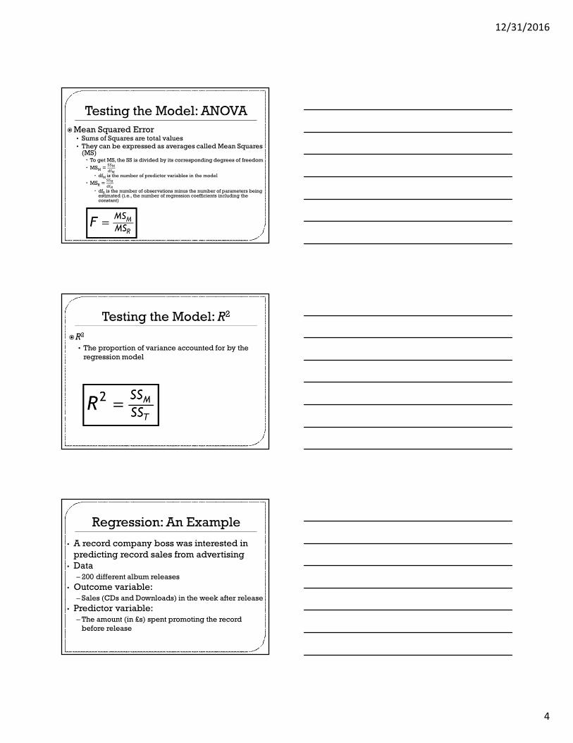
�Mean Squared Error• Sums of Squares are total values• They can be expressed as averages called Mean Squares

(MS)� To get MS, the SS is divided by its corresponding degrees of freedom

� MSM = ���

���

� dfM is the number of predictor variables in the model

� MSR = ���

���

� dfR is the number of observations minus the number of parameters being estimated (i.e., the number of regression coefficients including the constant)

�R2

• The proportion of variance accounted for by the

regression model

• A record company boss was interested in

predicting record sales from advertising

• Data

– 200 different album releases

• Outcome variable:

– Sales (CDs and Downloads) in the week after release

• Predictor variable:

– The amount (in £s) spent promoting the record

before release

12/31/2016

5

• Simple linear regression has a number of

distributional assumptions which can be

examined by looking at a residual plot (i.e., plot

showing the differences between the obtained

and predicted values of the criterion variable)1. The residuals should be normally distributed around the

predicted criterion scores (normality assumption)

2. The residuals should have a horizontal-line relationship with

predicted criterion scores (linearity assumption)

3. The variance of the residuals should be the same for all

predicted criterion scores (homoscedasticity assumption)

Plots of predicted values of the criterion

variable (Y) against residuals

A. Shows that the assumptions of regression

are met

B. Shows that the data fails to meet the

normality assumption

C. Shows that the data fails to meet the

linearity assumption

D. Shows that the data fails to meet the

homoscedasticity assumption

12/31/2016

6

12/31/2016

7

This is the R which reflects the degree of

association between our regression model

and the criterion variable

This is R2 which represents the amount of variance in the

criterion variable that is explained by the model (SSM)

relative to how much variance there was to explain in the

first place (SST). To express this value as a percentage, you

should multiply this value by 100 (which will tell you the

percentage of variation in the criterion variable that can be

explained by the model).

This is Adjusted R2 which corrects R2 for the number of

predictor variables included in the model. It will always be

less than or equal to R2. It is a more conservative estimate of

model fit because it penalizes researchers for including

predictor variables that are not strongly associated with the

criterion variable

12/31/2016

8

This is the standard error of the estimate which is a

measure of the accuracy of predictions. The larger the

standard error of the estimate, the more error in our

regression model

SSM

SSR

SST

MSR

MSM

The ANOVA tells us whether the model, overall, results in a

significantly good degree of prediction of the outcome

variable. However, the ANOVA does not tell us about the

individual contribution of variables in the model (although in

this simple case there is only one variable in the model which

allows us to infer that this variable is a good predictor)

This is the Y-intercept (i.e., the place

where the regression line intercepts

the Y-axis). This means that when £0

in advertising is spent, the model

predicts that 134,140 records will be

sold (unit of measurement is

“thousands of records”)

12/31/2016

9

This t-test compares the value of the Y-intercept with 0. If it is

significant, then it means that the value of the Y-intercept (134.14 in

this example) is significantly different from 0

This is the unstandardized slope or gradient coefficient. It is the

change in the outcome associated with a one unit change in the

predictor variable. This means that for every 1 point the advertising

budget is increased (unit of measurement is thousands of pounds)

the model predicts an increase of 96 records being sold (unit of

measurement for record sales was thousands of records)

This is the standardized regression coefficient (β). It represents the

strength of the association between the predictor and the criterion

variable. If there is only one predictor, then β is equal to the Pearson

product-moment correlation coefficient (the closer β is to +1 or -1,

then the better the prediction of Y from X [or X from Y])

12/31/2016

10

This t-test compares the magnitude of the standardized regression

coefficient (β) with 0. If it is significant, then it means that the value of

β (0.578 in this example) is significantly different from 0 (i.e., the

predictor variable is significantly associated with the criterion

variable)

� Y’ = A + BX� Record Sales = A + B(Advertising Budget)� Record Sales = 134.14 + (0.09612 x Advertising

Budget)� Expected record sales with £0 advertising budget

� 134.14 + (0.09612 x 0) = 134.14 + 0 = 134.14 = 134,140 records

� Expected record sales with £100,000 advertising budget

� 134.14 + (0.09612 x 100) = 134.14 + 9.612 = 143.752 = 143,752 records

� Expected record sales with £500,000 advertising budget

� 134.14 + (0.09612 x 500) = 134.14 + 48.06 = 182.2 = 182,200 records