psu ivy fundamentals of economics
TRANSCRIPT
7/21/2019 PSU IVY Fundamentals of Economics
http://slidepdf.com/reader/full/psu-ivy-fundamentals-of-economics 1/118
Fundamentals of Economics
Brian T. Kench,Ph.D.University of Tampa
Fifth Edition© Copyright 2011
Ivy Software
7/21/2019 PSU IVY Fundamentals of Economics
http://slidepdf.com/reader/full/psu-ivy-fundamentals-of-economics 2/118
TABLE OF CONTENTS
ABLE OF CONTENTS PAGE
Chapter One - Comparative Advantage and the Benefits of Trade..............1
Chapter Two - Demand & Supply..............................................................15
Chapter Three - he Costs of Production and Profit Maximization ..........43
Chapter Four - Economic Performance Metrics.........................................60
Chapter Five - Money & Banking...................................... .......................75
Chapter Six - Aggregate Demand & Aggregate Supply ............................87
Glossary........................................................................ ...........................102
Charts & Graphs.......................................................................................110

7/21/2019 PSU IVY Fundamentals of Economics
http://slidepdf.com/reader/full/psu-ivy-fundamentals-of-economics 3/118
CHAPTER ONEComparative Advantage and the Benefits of Trade
“Central to the globalization debate is the issue of the extent to which the United Statesshould compel the application of U.S. laws and regulatory standards to activities inother countries…. Most foreign governments resist these demands both because they areintrusions on the sovereign policies the countries have adopted with regard to regulation,and because to adopt American standards dramatically reduces a country’s comparativeadvantage to the detriment of its workers hoping to improve their lives” (emphasis added).
George L. Pr est, Wa Street Journa , A10, 6 18 04
1. Introduction
The concepts of opportunity cost and comparative advantage are two of the most important
concepts in all of economics. The opportunity cost of any life activity is the cost of what you giveup to partake in that activity. For example, the opportunity cost of reading this book might be notwatching your child’s baseball game. Among a comparison of individuals, businesses or countries,the one who has the lowest opportunity cost of an activity has a comparative advantage in thatactivity. Economists have long used these concepts to prove the mutual advantage of individuals,
businesses or countries specializing in things with which they have a comparative advantage andtrading for the rest. As the quote above reveals, these concepts are mechanisms that assist informedand educated debates on current public policy.
The following key concepts will be covered in this chapter: the four factors of production,opportunity cost, production possibilities frontier, increasing opportunity cost, absolute advantageand comparative advantage.
1
7/21/2019 PSU IVY Fundamentals of Economics
http://slidepdf.com/reader/full/psu-ivy-fundamentals-of-economics 4/118
2. Factors of Production
All the productive resources of the earth may be put in one of the following four categories:land, labor, capital, and entrepreneurial ability These four categories are collectively called thefactors of production The factors of production encompass all the possible productive resourcesused to produce goods and services. Moreover, the factors of production are all scarce economicresources because they are limited in supply.
The category of land includes all the gifts of nature – so called natural resources – that areused to produce goods and services. The category of abor includes work time and work effortthat people devote to producing goods and services. The category of capital includes all tools,instruments, machines, buildings, and other constructions that have been produced in the past that
businesses now use to produce goods and services. Finally, the category of entrepreneurial abilityincludes all human resources that organize the other factors of production. Entrepreneurs come upwith new ideas about what and how to produce, make business decisions, and bear the risks thatarise from these decisions .
Because the factors of production are limited in supply, they must be allocated amongmembers of human society. The price mechanism is one way, among several, that human societychooses to allocate scarce resources.
The market price of each factor of production has been assigned a unique name byeconomists. Rent is the unit price one pays for the use of land. Wage is the unit price one pays forthe services of labor. Interest is the unit price one pays for the use of capital. Profit is the incomeearned (or lost) by an entrepreneur for running a business.
3. Opportunity Cost and the Production Possibilities Frontier
The most fundamental principle in economics is opportunity cost The opportunity cost ofsomething is what you give up to get it. For example, you are currently using your time to earn agraduate degree; your opportunity cost of getting a graduate degree is missing time with friendsand family. In this section, the principle of opportunity cost is demonstrated by a productionpossibilities frontier. A production possibilities frontier is a model of an economy that shows howmuch the economy can produce using all of its factors of production efficiently.
2

7/21/2019 PSU IVY Fundamentals of Economics
http://slidepdf.com/reader/full/psu-ivy-fundamentals-of-economics 5/118
Figure 1-1roduction Possibilities Frontier
The economy in figure 1-1 produces only two goods: eggs and wine. The data in figure 1.1are the industrial output from one week of work. Each of the following is illustrated in the figure:
• If all the factors of production are employed to produce eggs, the economy is able to produce 82 eggs in a week.
• One the other hand, if all the factors of production are employed to produce wine, theeconomy is able to produce 10 bottles of wine per week.
• If all factors of production are fully and efficiently used, then the economy would beoperating somewhere on the production possibilities frontier.
• Points A, B, C, D, E and F each represent bundles of goods that lie on the economy’s production possibilities frontier.
When an economy does not fully use its factors of production, then it ends up at a locationinside the production possibilities frontier. If the economy ends up at the output bundle locatedat point “G”, the economy has not fully and efficiently used its factors of production. Lastly, thiseconomy does o have enough factors of production to produce bundle “H” or any bundle beyond
its production possibilities frontier.
�
�
�
�
�
�
�
�
�
�� �
�
3

7/21/2019 PSU IVY Fundamentals of Economics
http://slidepdf.com/reader/full/psu-ivy-fundamentals-of-economics 6/118
3.1 Example 1
Suppose the economy in figure 1-1 produces at point “B” – 80 eggs and one bottle of wine.If the economy chooses to move from point “B” to point “C” and produce another three bottles ofwine, it can now only produce 70 eggs. Therefore the opportunity cost of another three bottles ofwine equals 10 eggs (80 eggs – 70 eggs). In other words, the economy is giving up the productionof 10 eggs in order to produce another three bottles of wine.
3.2 Example 2
If the economy in figure 1-1 chooses to move from point “C” to point “D” and produceanother three bottles of wine, it may now only produce 50 eggs. The opportunity cost of producinganother three bottles of wine is 20 eggs (70 eggs – 50 eggs). Again, the economy is giving up the
production of 20 eggs in order to produce another three bottles of wine.
3.3 Example 3
Lastly, if the economy in figure 1-1 chooses to move from point “D” to point “F” and produce another three bottles of wine, it has zero factors of production left for the production ofeggs and can produce zero eggs. The opportunity cost of producing another three bottles of wineis 50 eggs (50 eggs – 0 eggs).
3.4 Increasing Opportunity Cost
As we increase the production of wine at a constant increment ( .e., by three bottles), the
opportunity cost of wine production increases. This is known as the law of ncreasing opportunitycost; it is reflected in the bowed-out shape of the production possibilities frontier in figure 1-1. Asmore and more of an economy’s factors of production are employed in the production of wine, theeconomy must sacrifice the production of eggs at an increasing rate.
Economic agents always start by using their best factors of production. Therefore, aneconomy experiences increasing opportunity cost as they increase one good’s production. In thecase of wine production, wine producers use their best fertilizer and their best machines to producethe first bottles of wine. The factors of production that are well-suited for wine production happen
to be the worst factors of production for the production of eggs. Thus, the opportunity cost of thefirst bottle of wine, in terms of eggs, is small. But as we increase our demand for bottles of wine,the economy must substitute out factors of production that are better suited for egg production anduse them to produce wine. The sacrifice in terms of eggs increases as additional bottles of wine are
produced.
4
7/21/2019 PSU IVY Fundamentals of Economics
http://slidepdf.com/reader/full/psu-ivy-fundamentals-of-economics 7/118
4. Absolute Advantage versus Comparative Advantage
To have an absolute advantage in something means that one has the lowest absolute production cost relative to those with whom they are compared. To have a comparative advantagein something means that one has the lowest opportunity cost relative to those with whom they arecompared.
David Ricardo first did the simple mathematics to demonstrate the concept of comparativeadvantage and the mutual advantage of trade in his 1817 book, The Principles of Political Economyand Taxation . Ricardo’s demonstration is one of the most important in all of economics and it isused as the root explanation for why
• one dines at a restaurant rather than cooking a meal at home;• one hires a landscaper to mow their lawn rather than mowing it for oneself;• Audi contracts with Bose Corporation to manufacture the sound system for its
automobiles rather than making the sound systems internally;• grocery stores in Boston, Massachusetts purchase oranges from Citrus Hills, Florida
rather than growing them in Boston; and• Sykes Corporation hires call centers in Bangalore, India, paying Indian employees
$2,100/year to answer consumer phone calls, rather than hiring employees in Tampa,Florida for a much higher wage year.
To help you get a better grasp of Ricardo’s analysis consider the following two examples.
5. Example 1: Elizabeth and Kyle
5.1 Self-Sufficiency
A self-sufficient individual makes everything that he needs in life from the factors of production with which he is endowed. Consider the following example in which Elizabeth andKyle each make wine and clothing: suppose that both Elizabeth and Kyle work a forty hour weekand both of them fully and efficiently use their endowed factors of production. Also assume that thethere is a constant opportunity cost between the production of a unit of wine and the productionof a unit of clothing. Because opportunity costs are constant and not increasing in this example,the production possibilities frontiers are linear and not bowed outward. This is done to simplify
our discussion.
5

7/21/2019 PSU IVY Fundamentals of Economics
http://slidepdf.com/reader/full/psu-ivy-fundamentals-of-economics 8/118
5.2 Elizabeth’s Production Possibilities Frontier
First consider Elizabeth. In forty hours, Elizabeth may produce 20 pieces of clothing r160 bottles of wine r any other combination that lies between these extremes on her production
possibilities frontier (PPF) in figure 1-2. If Elizabeth chooses to spend twenty hours making clothingand twenty hours making wine, then she would produce 10 pieces of clothing and 80 bottles ofwine. This bundle is located a point “A” in Elizabeth’s clothing and wine production possibilitiesfrontier for a forty-hour-work week.
igure 1-2Elizabeth’s Production Possibilities Frontier
Assume that Elizabeth fully and efficiently uses her factors of production. Therefore, shewill produce a bundle of wine and clothing that is on the production possibility frontier and will not
produce a bundle that is below the production possibilities frontier. Further, because she always produces somewhere on the production possibilities frontier, we can use figure 1-2 to determineElizabeth’s opportunity cost of producing a bottle of wine and her opportunity cost of producing aunit of clothing.
Suppose that Elizabeth produces 80 bottles of wine and 10 units of clothing, which is depictedwith point “A”. If Elizabeth changed her mind and decided that she wanted to produce 20 unitsof clothing, how many bottles of wine could she produce? The answer is zero. Elizabeth needsforty hours (all that she has) to produce 20 units of clothing, which leaves her no time to devote tothe production of bottles of wine in that week. The opportunity cost of making another 10 units ofclothing (from 10 units to 20 units) is 80 bottles of wine.
Using some simple math and the assumption of constant opportunity costs we can reduce andfigure out the opportunity cost of one unit of clothing. If 10 units of clothing have an opportunitycost of 80 bottles of wine, then one unit of clothing has an opportunity cost of eight bottles ofwine for Elizabeth By using algebra and solving for one bottle of wine, we can also prove that heopportunity cost of one bottle of wine is one-eighth of a unit of clothing for Elizabeth
�
�
� �
6
7/21/2019 PSU IVY Fundamentals of Economics
http://slidepdf.com/reader/full/psu-ivy-fundamentals-of-economics 9/118
In economic terms this means that if Elizabeth decides to produce one additional bottle ofwine, she will use up the factors of production that would have been used to produce one-eighthof a unit of clothing. If she decides to produce one additional unit of clothing, she will use up thefactors of production that would have been used to produce eight bottles of wine.
5.3 Kyle’s Production Possibilities Frontier
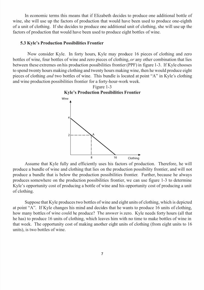
ow consider Kyle. In forty hours, Kyle may produce 16 pieces of clothing and zero bottles of wine, four bottles of wine and zero pieces of clothing, or any other combination that lies between these extremes on his production possibilities frontier (PPF) in figure 1-3. If Kyle choosesto spend twenty hours making clothing and twenty hours making wine, then he would produce eight
pieces of clothing and two bottles of wine. This bundle is located at point “A” in Kyle’s clothingand wine production possibilities frontier for a forty-hour-work week.
Figure 1-3Kyle’s Production Possibilities Frontier
Assume that Kyle fully and efficiently uses his factors of production. Therefore, he will produce a bundle of wine and clothing that lies on the production possibility frontier, and will not produce a bundle that is below the production possibilities frontier. Further, because he always produces somewhere on the production possibilities frontier, we can use figure 1-3 to determineKyle’s opportunity cost of producing a bottle of wine and his opportunity cost of producing a unitof clothing.
Suppose that Kyle produces two bottles of wine and eight units of clothing, which is depictedat point “A”. If Kyle changes his mind and decides that he wants to produce 16 units of clothing,how many bottles of wine could he produce? The answer is zero. Kyle needs forty hours (all thathe has) to produce 16 units of clothing, which leaves him with no time to make bottles of wine inthat week. The opportunity cost of making another eight units of clothing (from eight units to 16units), is two bottles of wine.
�
7
7/21/2019 PSU IVY Fundamentals of Economics
http://slidepdf.com/reader/full/psu-ivy-fundamentals-of-economics 10/118
Using some simple math and the assumption of constant opportunity costs, we can reduce andfigure out the opportunity cost of one unit of clothing. If eight units of clothing have an opportunitycost of two bottles of wine, then one unit of clothing has an opportunity cost of one-fourth of abottle of wine for Kyle . By using algebra and solving for one bottle of wine, we can show that theopportunity cost of one bottle of wine is four units of clothing for Kyle
In economic terms this means that if he wants to produce one unit of clothing, he mustsacrifice the resources needed to produce one-fourth of a bottle of wine. And if Kyle wants to
produce one bottle of wine, then he must sacrifice the resources needed to produce four units ofclothing.
5.4 Absolute Advantage and Comparative Advantage
Does Elizabeth or Kyle have an absolute advantage in the production of wine? Elizabethcan produce more wine over the course of forty hours relative to Kyle (160 bottles for Elizabethversus four bottles for Kyle). Therefore, Elizabeth has an absolute advantage in the production ofwine .
Does Elizabeth or Kyle have an absolute advantage in the production of clothing? Elizabethcan produce more clothing over the course of forty hours relative to Kyle (20 units of clothing forElizabeth versus 16 units of clothing for Kyle). Therefore, Elizabeth has an absolute advantage inthe production of clothing, too .
Although it is clear that Elizabeth is better at producing wine and clothing relative to Kyle,the concept of absolute advantage tells us nothing about whether or not Elizabeth or Kyle might
benefit from specializing in the production of one of the two goods and trading for the other. Andlet us not be shy here, trading in this context is fully analogous to outsourcing in contemporary
business language. The concept that can help inform Elizabeth and Kyle about the benefits of tradeis the concept of comparative advantage.
The concept of comparative advantage states that when comparing producers, the one withthe lowest opportunity cost in the production of some good or service has a comparative advantagein the production of that good or service. In our problem, who has a comparative advantage in the
production of a bottle of wine? Who has a comparative advantage in the production of clothing?
First, let’s look at the production of wine. Elizabeth’s opportunity cost of producing one bottle of wine is one-eighth of a unit of clothing and Kyle’s opportunity cost of producing one bottle of wine was four units of clothing. Therefore, Elizabeth has a comparative advantage in the production of wine because she has to give up less clothing (one-eighth of a unit versus four unitsof clothing) to make one bottle of wine .
8
7/21/2019 PSU IVY Fundamentals of Economics
http://slidepdf.com/reader/full/psu-ivy-fundamentals-of-economics 11/118
What about clothing? Elizabeth’s opportunity cost of producing one unit of clothing is eight bottles of wine and Kyle’s opportunity cost of producing one unit of clothing is one-fourth of a bottle of wine. Therefore, Kyle has a comparative advantage in the production of clothing becausehe has to give up less wine (one-fourth of a bottle versus eight bottles of wine) to make one unit ofclothing .
5.5 Trade
An individual or a business should specialize in the production of a good or service in whichthey have a comparative advantage. Below we will prove why this is always the correct thing todo. In our current problem, we have discovered that Elizabeth has a comparative advantage in the
production of wine and Kyle has a comparative advantage in the production of clothing. With thisinformation, we may conclude that Elizabeth should specialize in the production of wine and tradefor clothing and Kyle should specialize in the production of clothing and trade for wine.
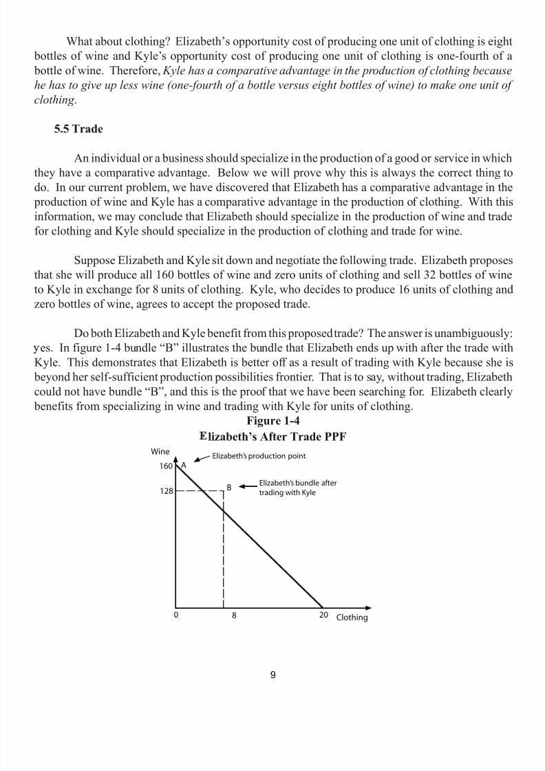
Suppose Elizabeth and Kyle sit down and negotiate the following trade. Elizabeth proposesthat she will produce all 160 bottles of wine and zero units of clothing and sell 32 bottles of wineto Kyle in exchange for 8 units of clothing. Kyle, who decides to produce 16 units of clothing andzero bottles of wine, agrees to accept the proposed trade.
Do both Elizabeth and Kyle benefit from this proposed trade? The answer is unambiguously:es. In figure 1-4 bundle “B” illustrates the bundle that Elizabeth ends up with after the trade with
Kyle. This demonstrates that Elizabeth is better off as a result of trading with Kyle because she is beyond her self-sufficient production possibilities frontier. That is to say, without trading, Elizabethcould not have bundle “B”, and this is the proof that we have been searching for. Elizabeth clearly
benefits from specializing in wine and trading with Kyle for units of clothing.Figure 1-4
lizabeth’s After Trade PPF
�
�
9
7/21/2019 PSU IVY Fundamentals of Economics
http://slidepdf.com/reader/full/psu-ivy-fundamentals-of-economics 12/118
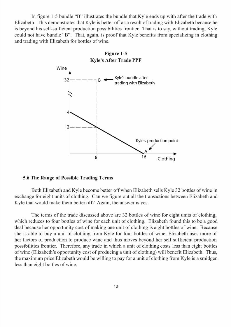
In figure 1-5 bundle “B” illustrates the bundle that Kyle ends up with after the trade withElizabeth. This demonstrates that Kyle is better off as a result of trading with Elizabeth because heis beyond his self-sufficient production possibilities frontier. That is to say, without trading, Kylecould not have bundle “B”. That, again, is proof that Kyle benefits from specializing in clothingand trading with Elizabeth for bottles of wine.
Figure 1-5Kyle’s After Trade PPF
5.6 The Range of Possible Trading Terms
Both Elizabeth and Kyle become better off when Elizabeth sells Kyle 32 bottles of wine inexchange for eight units of clothing. Can we figure out all the transactions between Elizabeth andKyle that would make them better off? Again, the answer is yes.
The terms of the trade discussed above are 32 bottles of wine for eight units of clothing,which reduces to four bottles of wine for each unit of clothing. Elizabeth found this to be a good
deal because her opportunity cost of making one unit of clothing is eight bottles of wine. Becauseshe is able to buy a unit of clothing from Kyle for four bottles of wine, Elizabeth uses more ofher factors of production to produce wine and thus moves beyond her self-sufficient production
possibilities frontier. Therefore, any trade in which a unit of clothing costs less than eight bottlesof wine (Elizabeth’s opportunity cost of producing a unit of clothing) will benefit Elizabeth. Thus,the maximum price Elizabeth would be willing to pay for a unit of clothing from Kyle is a smidgenless than eight bottles of wine.
�
�
10
7/21/2019 PSU IVY Fundamentals of Economics
http://slidepdf.com/reader/full/psu-ivy-fundamentals-of-economics 13/118
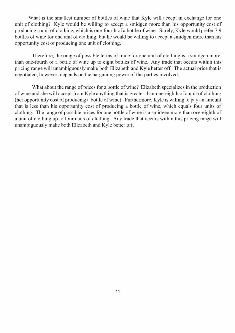
What is the smallest number of bottles of wine that Kyle will accept in exchange for oneunit of clothing? Kyle would be willing to accept a smidgen more than his opportunity cost of
producing a unit of clothing, which is one-fourth of a bottle of wine. Surely, Kyle would prefer 7.9 bottles of wine for one unit of clothing, but he would be willing to accept a smidgen more than hisopportunity cost of producing one unit of clothing.
Therefore, the range of possible terms of trade for one unit of clothing is a smidgen morethan one-fourth of a bottle of wine up to eight bottles of wine. Any trade that occurs within this pricing range will unambiguously make both Elizabeth and Kyle better off. The actual price that isnegotiated, however, depends on the bargaining power of the parties involved.
What about the range of prices for a bottle of wine? Elizabeth specializes in the productionof wine and she will accept from Kyle anything that is greater than one-eighth of a unit of clothing(her opportunity cost of producing a bottle of wine). Furthermore, Kyle is willing to pay an amountthat is less than his opportunity cost of producing a bottle of wine, which equals four units ofclothing. The range of possible prices for one bottle of wine is a smidgen more than one-eighth ofa unit of clothing up to four units of clothing. Any trade that occurs within this pricing range willunambiguously make both Elizabeth and Kyle better off.
11
7/21/2019 PSU IVY Fundamentals of Economics
http://slidepdf.com/reader/full/psu-ivy-fundamentals-of-economics 14/118
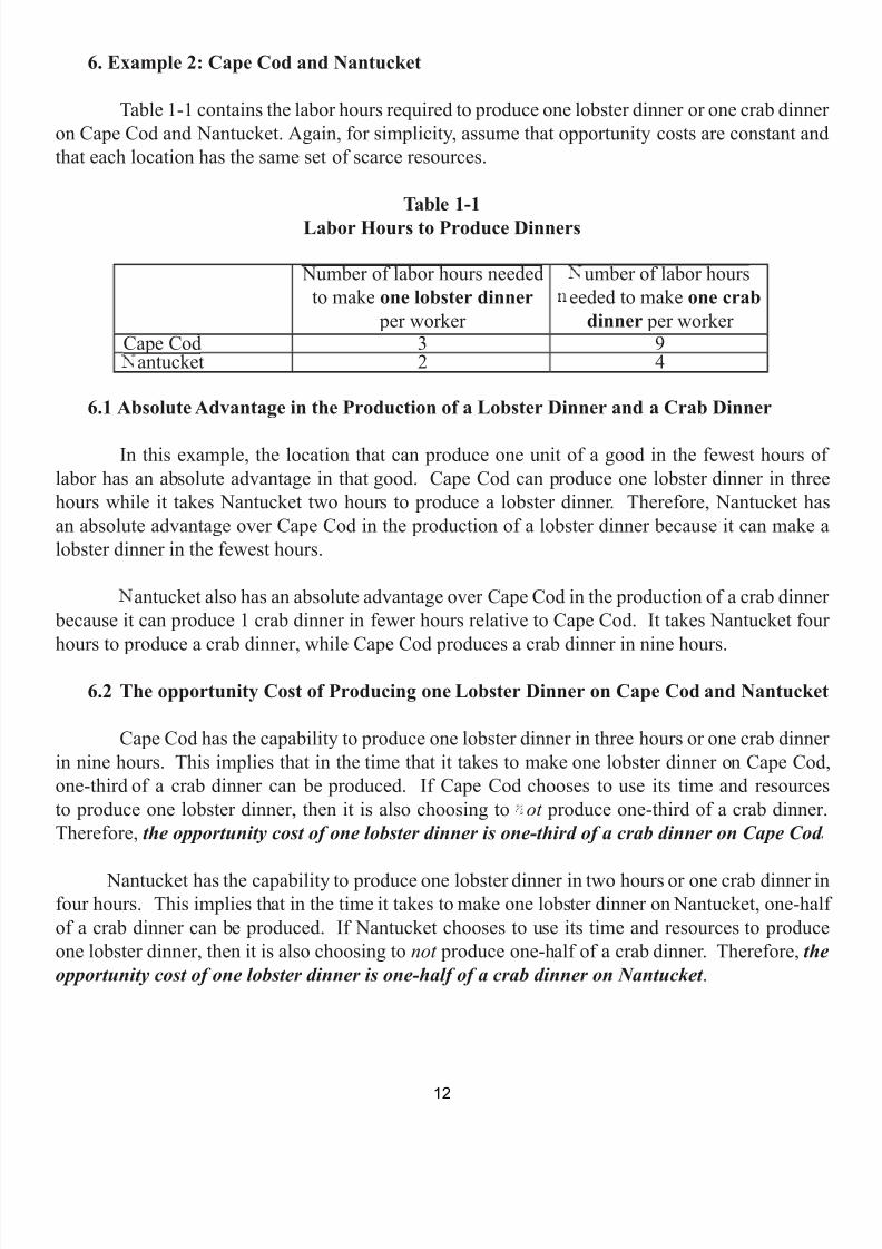
6. Example 2: Cape Cod and Nantucket
Table 1-1 contains the labor hours required to produce one lobster dinner or one crab dinneron Cape Cod and Nantucket. Again, for simplicity, assume that opportunity costs are constant andthat each location has the same set of scarce resources.
Table 1-1Labor Hours to Produce Dinners
Number of labor hours neededto make one lobster dinner
per worker
umber of labor hourseeded to make one crab
dinner per worker Cape Cod 3 9
antucket 2 4
6.1 Absolute Advantage in the Production of a Lobster Dinner and a Crab Dinner
In this example, the location that can produce one unit of a good in the fewest hours oflabor has an absolute advantage in that good. Cape Cod can produce one lobster dinner in threehours while it takes Nantucket two hours to produce a lobster dinner. Therefore, Nantucket hasan absolute advantage over Cape Cod in the production of a lobster dinner because it can make alobster dinner in the fewest hours.
antucket also has an absolute advantage over Cape Cod in the production of a crab dinner because it can produce 1 crab dinner in fewer hours relative to Cape Cod. It takes Nantucket fourhours to produce a crab dinner, while Cape Cod produces a crab dinner in nine hours.
6.2 The opportunity Cost of Producing one Lobster Dinner on Cape Cod and Nantucket
Cape Cod has the capability to produce one lobster dinner in three hours or one crab dinnerin nine hours. This implies that in the time that it takes to make one lobster dinner on Cape Cod,one-third of a crab dinner can be produced. If Cape Cod chooses to use its time and resourcesto produce one lobster dinner, then it is also choosing to ot produce one-third of a crab dinner.Therefore, the opportunity cost of one lobster dinner is one-third of a crab dinner on Cape Cod
Nantucket has the capability to produce one lobster dinner in two hours or one crab dinner infour hours. This implies that in the time it takes to make one lobster dinner on Nantucket, one-half of a crab dinner can be produced. If Nantucket chooses to use its time and resources to produceone lobster dinner, then it is also choosing to not produce one-half of a crab dinner. Therefore, theopportunity cost of one lobster dinner is one-half of a crab dinner on Nantucket .
12
7/21/2019 PSU IVY Fundamentals of Economics
http://slidepdf.com/reader/full/psu-ivy-fundamentals-of-economics 15/118
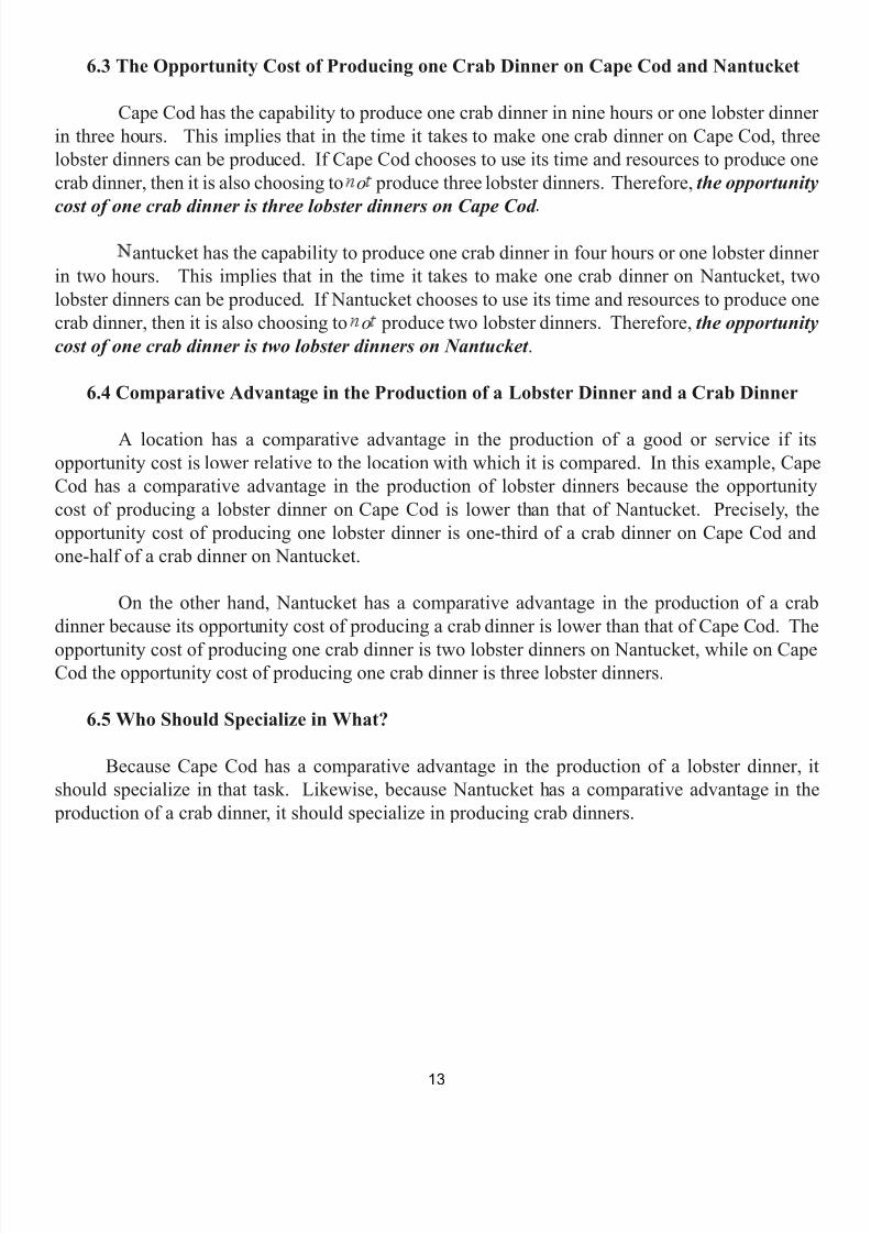
6.3 The Opportunity Cost of Producing one Crab Dinner on Cape Cod and Nantucket
Cape Cod has the capability to produce one crab dinner in nine hours or one lobster dinnerin three hours. This implies that in the time it takes to make one crab dinner on Cape Cod, threelobster dinners can be produced. If Cape Cod chooses to use its time and resources to produce onecrab dinner, then it is also choosing to o produce three lobster dinners. Therefore, the opportunity
cost of one crab dinner is three lobster dinners on Cape Cod antucket has the capability to produce one crab dinner in four hours or one lobster dinner
in two hours. This implies that in the time it takes to make one crab dinner on Nantucket, twolobster dinners can be produced. If Nantucket chooses to use its time and resources to produce onecrab dinner, then it is also choosing to o produce two lobster dinners. Therefore, the opportunitycost of one crab dinner is two lobster dinners on Nantucket .
6.4 Comparative Advantage in the Production of a Lobster Dinner and a Crab Dinner
A location has a comparative advantage in the production of a good or service if itsopportunity cost is lower relative to the location with which it is compared. In this example, CapeCod has a comparative advantage in the production of lobster dinners because the opportunitycost of producing a lobster dinner on Cape Cod is lower than that of Nantucket. Precisely, theopportunity cost of producing one lobster dinner is one-third of a crab dinner on Cape Cod andone-half of a crab dinner on Nantucket.
On the other hand, Nantucket has a comparative advantage in the production of a crabdinner because its opportunity cost of producing a crab dinner is lower than that of Cape Cod. The
opportunity cost of producing one crab dinner is two lobster dinners on Nantucket, while on CapeCod the opportunity cost of producing one crab dinner is three lobster dinners.
6.5 Who Should Specialize in What?
Because Cape Cod has a comparative advantage in the production of a lobster dinner, itshould specialize in that task. Likewise, because Nantucket has a comparative advantage in the
production of a crab dinner, it should specialize in producing crab dinners.
13

7/21/2019 PSU IVY Fundamentals of Economics
http://slidepdf.com/reader/full/psu-ivy-fundamentals-of-economics 16/118
6.6 The Range of Possible Prices for a Lobster Dinner and a Crab Dinner
Because Cape Cod has a comparative advantage in the production of a lobster dinner, itwill specialize in the production of that good. Cape Cod will benefit from trading with Nantucketwhenever they receive more than one-third of a crab dinner for a lobster dinner. Again, this is true
because one-third of a crab dinner is the opportunity cost of producing one lobster dinner on CapeCod.
antucket, too, will benefit by purchasing lobster dinners from Cape Cod, so long as the price they pay is lower then its opportunity cost of producing a lobster dinner. Recall, that theopportunity cost of producing a lobster dinner on Nantucket is one-half of a crab dinner.
Therefore, the range of possible prices for one lobster dinner is a smidgen larger than one-third of a crab dinner (Cape Cod’s opportunity cost of making a lobster dinner) up to a smidgenless than one-half of a crab dinner (Nantucket’s opportunity cost of making a lobster dinner). Anytrade that occurs within this pricing range will unambiguously make both Cape Cod and Nantucket
better off because they will move to a location beyond their self-sufficient production possibilitiesfrontier.
antucket has a comparative advantage in the production of a crab dinner, and it willspecialize in the production of that good. Nantucket will benefit from trade with Cape Cod wheneverit receives more than two lobster dinners for each crab dinner. Again, this is true because twolobster dinners is the opportunity cost of producing a crab dinner on Nantucket.
Here, too, Cape Cod, benefits by purchasing crab dinners from Nantucket, so long as the
price paid is lower then its opportunity cost of producing a crab dinner. Again, the opportunity costof producing one crab dinner on Cape Cod is three lobster dinners.
Therefore, the range of possible prices for one crab dinner is a smidgen more than twolobster dinners (Nantucket’s opportunity cost of making a crab dinner) up a bit less than three lobsterdinners (Cape Cod’s opportunity cost of making a crab dinner). Any trade that occurs within this
pricing range will unambiguously make both Nantucket and Cape Cod better off because they willmove to a location beyond their self-sufficient production possibilities frontier.
14
7/21/2019 PSU IVY Fundamentals of Economics
http://slidepdf.com/reader/full/psu-ivy-fundamentals-of-economics 17/118
CH PTER T ODeman & Supp y
1. Introduction
This chapter introduces the odel of demand and supply . Economists use the model ofdemand and supply to analyze how buyers and sellers interact in the marketplace. It shows howmarket prices are determined and it demonstrates how many units of a good or service will be
bought and sold. Examples of markets include EBay.com, the New York Stock Exchange, therestaurant market, the gasoline market, and furniture market. Markets are everywhere.
The following key concepts will be covered in this chapter: a demand schedule, a demandcurve, a demand function, the law of demand, the market demand curve, the market demand schedule,the price elasticity of demand, the cross price elasticity of demand, the income elasticity of demand,
a supply schedule, a supply curve, a supply function, the law of supply, the market supply curve, themarket supply schedule, the elasticity of supply, and comparative-static analysis.
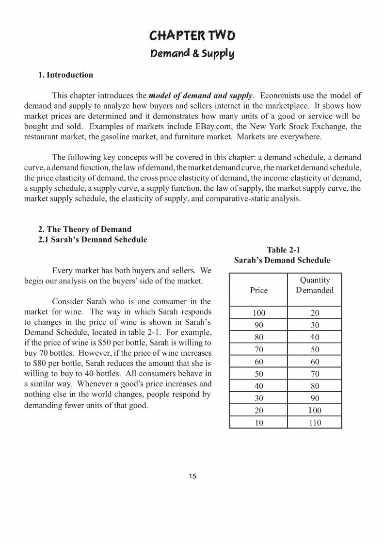
2. The Theory of Demand2.1 Sarah’s Demand Schedule
Table 2-1 Sarah’s Demand Schedule
Every market has both buyers and sellers. We begin our analysis on the buyers’ side of the market.
Consider Sarah who is one consumer in themarket for wine. The way in which Sarah respondsto changes in the price of wine is shown in Sarah’sDemand Schedule, located in table 2-1. For example,if the price of wine is $50 per bottle, Sarah is willing to
buy 70 bottles. However, if the price of wine increasesto $80 per bottle, Sarah reduces the amount that she iswilling to buy to 40 bottles. All consumers behave ina similar way. Whenever a good’s price increases andnothing else in the world changes, people respond bydemanding fewer units of that good.
PriceQuantityemanded
100 2090 3080 070 5060 6050 7040 8030 9020 0010 110
15
7/21/2019 PSU IVY Fundamentals of Economics
http://slidepdf.com/reader/full/psu-ivy-fundamentals-of-economics 18/118
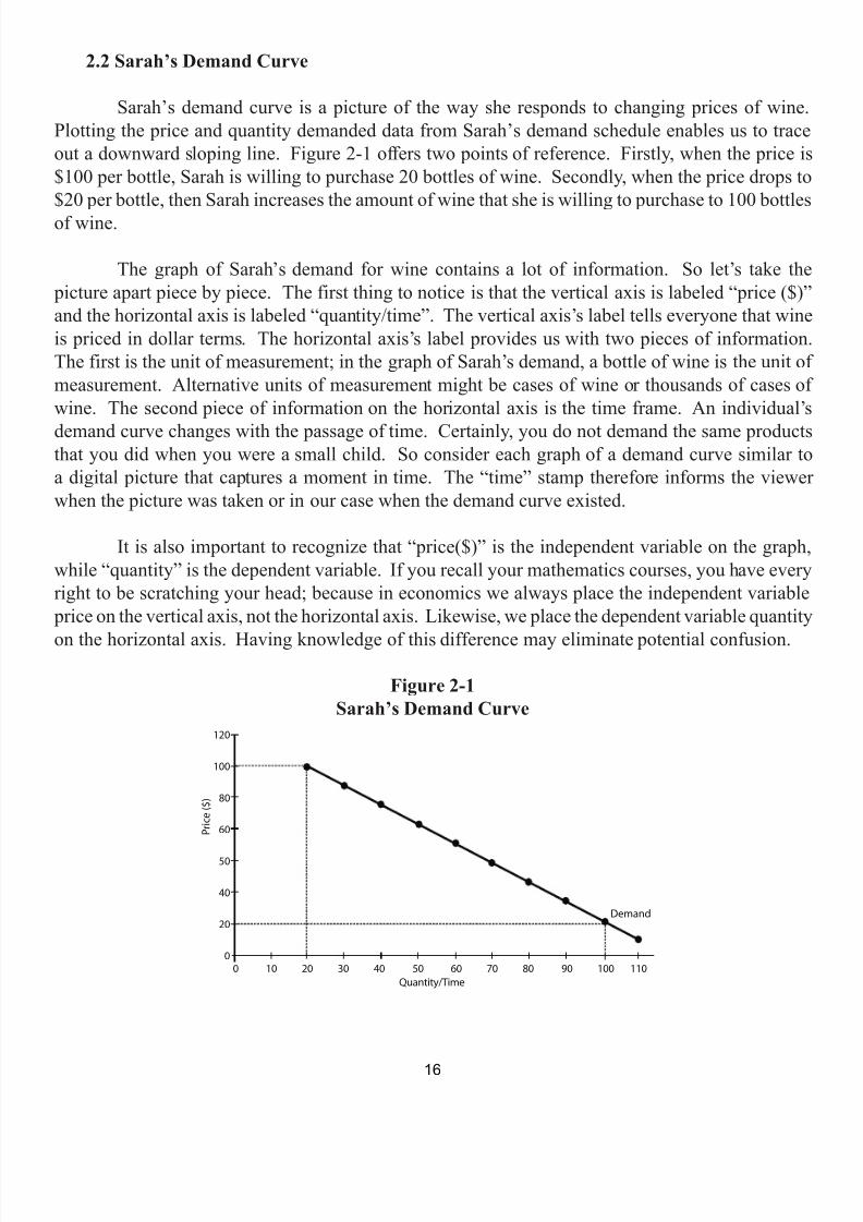
2.2 Sarah’s Demand Curve
Sarah’s demand curve is a picture of the way she responds to changing prices of wine.Plotting the price and quantity demanded data from Sarah’s demand schedule enables us to traceout a downward sloping line. Figure 2-1 offers two points of reference. Firstly, when the price is$100 per bottle, Sarah is willing to purchase 20 bottles of wine. Secondly, when the price drops to$20 per bottle, then Sarah increases the amount of wine that she is willing to purchase to 100 bottlesof wine.
The graph of Sarah’s demand for wine contains a lot of information. So let’s take the picture apart piece by piece. The first thing to notice is that the vertical axis is labeled “price ($)”and the horizontal axis is labeled “quantity/time”. The vertical axis’s label tells everyone that wineis priced in dollar terms. The horizontal axis’s label provides us with two pieces of information.The first is the unit of measurement; in the graph of Sarah’s demand, a bottle of wine is the unit ofmeasurement. Alternative units of measurement might be cases of wine or thousands of cases ofwine. The second piece of information on the horizontal axis is the time frame. An individual’sdemand curve changes with the passage of time. Certainly, you do not demand the same productsthat you did when you were a small child. So consider each graph of a demand curve similar toa digital picture that captures a moment in time. The “time” stamp therefore informs the viewerwhen the picture was taken or in our case when the demand curve existed.
It is also important to recognize that “price($)” is the independent variable on the graph,while “quantity” is the dependent variable. If you recall your mathematics courses, you have everyright to be scratching your head; because in economics we always place the independent variable
price on the vertical axis, not the horizontal axis. Likewise, we place the dependent variable quantity
on the horizontal axis. Having knowledge of this difference may eliminate potential confusion.
Figure 2-1Sarah’s Demand Curve
�
��
�
�
�
�
�
�
�
�
16
7/21/2019 PSU IVY Fundamentals of Economics
http://slidepdf.com/reader/full/psu-ivy-fundamentals-of-economics 19/118
2.3 Sarah’s Demand Function
Sarah’s quantity demanded of wine depends on independent variables other than the priceof wine. Some of the more influential variables are the rices of complementary goods and theprices of substitute goods
• Complementary goods. Because Sarah likes to eat Gouda cheese and wheat crackersas she drinks wine, she considers them complementary goods to wine. Thus, Sarahconsiders the price of Gouda cheese and the price of wheat crackers when she decideshow many bottles of wine she is willing to buy at any given price.
• Substitute goods. Sarah enjoys drinking wine, Tanqueray gin, and other fine liquors andshe considers these beverages substitutes for one another. Thus, Sarah considers the priceof Tanqueray gin and the price of other fine liquors when she decides how many bottlesof wine she is willing to buy at any given price.
Another factor affecting Sarah’s demand for wine is her income.
• If wine is a normal good , then positive changes in income will induce Sarah to purchasemore bottles of wine at any given price.
• If wine is an inferior good for Sarah, then positive changes in income will induce Sarahto purchase fewer bottles of wine at any given price.
Does Sarah enjoy drinking wine? Obviously this matters, too. Economists lump measures
of satisfaction, enjoyment, pleasure, tc. into the category “ astes and preferences .
• For example, after Sarah discovers that she enjoys a particular vineyard and vintage ofwine, she reveals through her market behavior that she is now willing to purchase more
bottles of this wine at any given price.
• If she drinks a different brand of wine and finds it horribly bad, then she will reveal thatshe is willing to buy fewer bottles of that wine at any given price.
One other important category is Sarah’s expectations of the future Suppose that Sarahunexpectedly discovers that her favorite wine and vintage is soon to run-out. Because of this newinformation, Sarah reveals that she is now willing to buy more bottles at any given price. Anexample of this behavior occured when hurricanes Katrina and Rita blew ashore in the U.S. in2005. Buyers hoarded gasoline - that is, they bought more gasoline at every given price relative to
before the storms developed - because they expected gasoline shortages after the storms.
17
7/21/2019 PSU IVY Fundamentals of Economics
http://slidepdf.com/reader/full/psu-ivy-fundamentals-of-economics 20/118
All of these variables may be succinctly expressed in the following general equation, wheresignifies a general function:
Q = f (P ;P ,P ,I,T & P, E)Sarah’s quantity demanded of wine is a number, say 15 bottles, and it is the dependent
variable which depends on many independent variables. The quantity demanded depends, foremost,on the market price of a bottle of wine (P ne). The price of wine is an independent variable becauseit is determined by the wine market. The other independent variables that affect Sarah’s quantitydemanded of wine are the price of complements (P comp ement ), the price of substitutes (P u st tute ), income(I), tastes and preferences (T & P), and expectations of the future (E).
2.4 The Law of Demand
Unlike Sarah’s quantity demanded of wine, which is a number, her demand or wine is a
set of numbers. It is a relationship that reveals how many bottles of wine she demands at each andevery price of wine.
Consider this question: What is Sarah’s quantity demanded of wine when the price is $90 per bottle? In order to get a simple answer to this question we have to make an assumption: theceteris paribus assumption. eteris paribus is a Latin phrase that means other things equal. Forour purposes, when the eteris paribus assumption is imposed, every independant variable exceptthe price of wine is held constant.
The eteris paribus assumption is analogous to taking a digital picture of the marketplace,whereby you stop the market in both time and space. Once all motion stops, we may more easilyanalyze the marketplace. In particular, we can discover how many bottles of wine Sarah willdemand when the price is $9.
If the price of wine decreases, then ceteris paribus the quantity demanded of wine willincrease. The reverse is also true. If the price of wine increases, then ceteris paribus the quantitydemanded of wine will decrease. This negative relationship between the price of wine and thequantity demanded always holds true – it is called the law of demand
demanded wine
18
7/21/2019 PSU IVY Fundamentals of Economics
http://slidepdf.com/reader/full/psu-ivy-fundamentals-of-economics 21/118
2.5 Shifts of the Demand Curve
The demand curve shifts only when there is a change in one of the independent variablesheld fixed under the eteris paribus assumption. Therefore, the demand curve shifts only when asecond proverbial digital photo of the marketplace is taken. Something other than the price of winehas to be different in some way for the demand curve for wine to shift. There are no exceptions to
this ruleMoreover, a demand curve shift only to the south-west or to the orth-east For example,
if the price of Gouda cheese, a omplement to wine, increases, then Sarah is willing to buy fewer bottles of wine at any given price. Because of the increase in the price of Gouda cheese, Sarah’sdemand curve for wine shifts to the south-west. This is so because Sarah likes wine and cheesetogether and the more expensive cheese is, the fewer blocks of cheese and bottles of wine she will
buy.
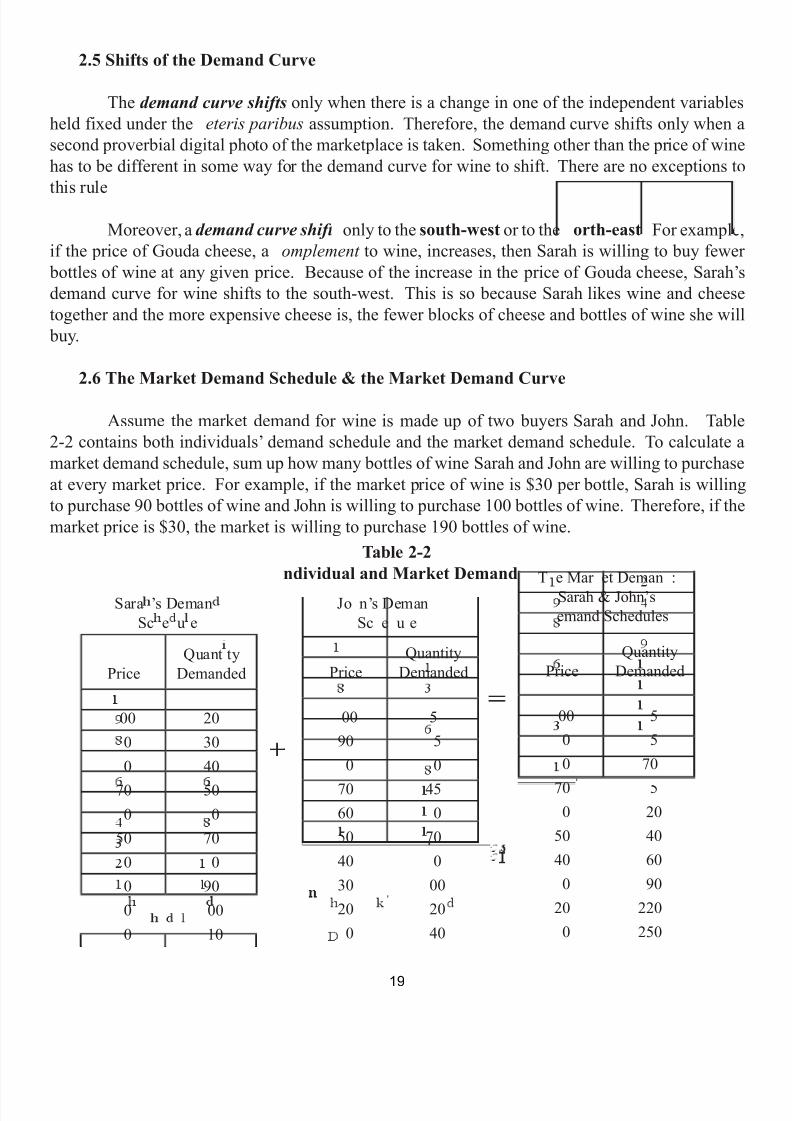
2.6 The Market Demand Schedule & the Market Demand Curve
Assume the market demand for wine is made up of two buyers Sarah and John. Table2-2 contains both individuals’ demand schedule and the market demand schedule. To calculate amarket demand schedule, sum up how many bottles of wine Sarah and John are willing to purchaseat every market price. For example, if the market price of wine is $30 per bottle, Sarah is willingto purchase 90 bottles of wine and John is willing to purchase 100 bottles of wine. Therefore, if themarket price is $30, the market is willing to purchase 190 bottles of wine.
Table 2-2ndividual and Market Demand
PriceQuant ty
Demanded
00 200 300 40
70 500 0
50 700 00 900 000 10
PriceQuantity
Demanded
00 590 5
0 0
70 4560 050 7040 030 0020 20
0 40
PriceQuantity
Demanded
00 50 50 70
70 50 20
50 4040 60
0 9020 220
0 250
Sara ’s DemanSc e u e
Jo n’s DemanSc e u e
T e Mar et Deman :Sarah & John’semand Schedules
19

7/21/2019 PSU IVY Fundamentals of Economics
http://slidepdf.com/reader/full/psu-ivy-fundamentals-of-economics 22/118
The market demand function (below) contains one additional independent variable: thenumber of buyers in the market . As the number of buyers in the market increases, ceteris
paribus the market demand curve shifts to the north-east. And if the umber of buyers in themarket decreases, ceteris paribus , the market demand curve shifts to the south-west.
= f (P ;P ,P ,I,T & P, E,# of Buyers)
The horizontal summation of Sarah and John’s demand curves yields the market demandcurve and it is depicted in figure 2-2.
igure 2-2arket Demand Curve
ne
��
�
�
�
�
�
�
�
�
�
�
�
�
Market Demand Curve
20
7/21/2019 PSU IVY Fundamentals of Economics
http://slidepdf.com/reader/full/psu-ivy-fundamentals-of-economics 23/118
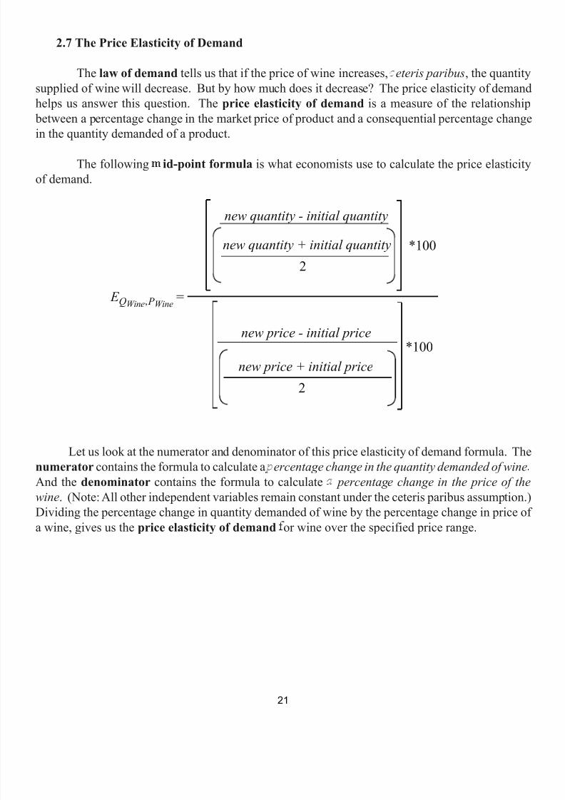
2.7 The Price Elasticity of Demand
The law of demand tells us that if the price of wine increases, eteris paribus , the quantitysupplied of wine will decrease. But by how much does it decrease? The price elasticity of demandhelps us answer this question. The price elasticity of demand is a measure of the relationship
between a percentage change in the market price of product and a consequential percentage change
in the quantity demanded of a product.The following id-point formula is what economists use to calculate the price elasticity
of demand.
Let us look at the numerator and denominator of this price elasticity of demand formula. Thenumerator contains the formula to calculate a ercentage change in the quantity demanded of wineAnd the denominator contains the formula to calculate percentage change in the price of thewine . (Note: All other independent variables remain constant under the ceteris paribus assumption.)Dividing the percentage change in quantity demanded of wine by the percentage change in price ofa wine, gives us the price elasticity of demand or wine over the specified price range.
new quantity - initial quantity
new quantity + initial quantity
new price - initial price
new price + initial price2
2
*100
*100
E QWine , P Wine
=,
21
7/21/2019 PSU IVY Fundamentals of Economics
http://slidepdf.com/reader/full/psu-ivy-fundamentals-of-economics 24/118
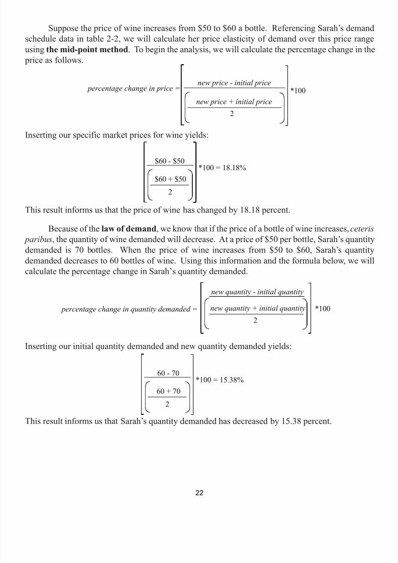
Suppose the price of wine increases from $50 to $60 a bottle. Referencing Sarah’s demandschedule data in table 2-2, we will calculate her price elasticity of demand over this price rangeusing the mid-point method . To begin the analysis, we will calculate the percentage change in the
price as follows.
Inserting our specific market prices for wine yields:
This result informs us that the price of wine has changed by 18.18 percent.
Because of the law of demand , we know that if the price of a bottle of wine increases, ceteris paribus , the quantity of wine demanded will decrease. At a price of $50 per bottle, Sarah’s quantitydemanded is 70 bottles. When the price of wine increases from $50 to $60, Sarah’s quantitydemanded decreases to 60 bottles of wine. Using this information and the formula below, we willcalculate the percentage change in Sarah’s quantity demanded.
Inserting our initial quantity demanded and new quantity demanded yields:
This result informs us that Sarah’s quantity demanded has decreased by 15.38 percent.
new price - initial price
new price + initial price2
*100 percentage change in price =
$60 - $50
$60 + $50
2
*100 = 18.18%
new quantity - initial quantity
new quantity + initial quantity2
*100 percentage change in quantity demanded =
60 - 70
60 + 70
2
*100 = 15.38%
22
7/21/2019 PSU IVY Fundamentals of Economics
http://slidepdf.com/reader/full/psu-ivy-fundamentals-of-economics 25/118
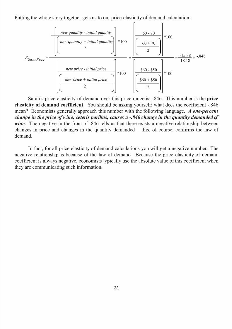
Putting the whole story together gets us to our price elasticity of demand calculation:
Sarah’s price elasticity of demand over this price range is -.846. This number is the priceelasticity of demand coefficient . You should be asking yourself: what does the coefficient -.846mean? Economists generally approach this number with the following language. A one-percentchange in the price of wine, ceteris paribus, causes a -.846 change in the quantity demanded owine. The negative in the front of .846 tells us that there exists a negative relationship betweenchanges in price and changes in the quantity demanded – this, of course, confirms the law ofdemand.
In fact, for all price elasticity of demand calculations you will get a negative number. Thenegative relationship is because of the law of demand Because the price elasticity of demandcoefficient is always negative, economists ypically use the absolute value of this coefficient whenthey are communicating such information
new quantity - initial quantity
new quantity + initial quantity
new price - initial price
new price + initial price2
2
*100
*100
E QWine , P Wine =
60 - 70
60 + 70
2
*100
$60 - $50
$60 + $50
2
*100
� �
-15.3818.18
� -.846,
23
7/21/2019 PSU IVY Fundamentals of Economics
http://slidepdf.com/reader/full/psu-ivy-fundamentals-of-economics 26/118
Here is a second question you should be asking yourself: does the size of the number matter?In this case, size does matter. Consider the following three categories that economists use to analyzea price elasticity of demand calculation.
The first price elasticity of demand category is a coefficient with an absolute value of lessthan one . If the price elasticity of demand has an absolute value of less than one, then the demandcurve is inelastic around the prices analyzed. In this category, a one-percent price change generatesa less than one-percent change in the quantity demanded. When the demand curve is inelastic,consumers do not radically change their quantity demanded when the market price changes. Forexample, consumers of insulin (a product that diabetics need to live) do no change their consumptionof insulin when the price of insulin changes. Insulin consumers are not responsive to price changes
because there are few substitute goods available.
The second price elasticity of demand category is a coefficient with an absolute value of greater than one . If the price elasticity of demand has an absolute value of greater than one,then the demand curve is elastic around the prices analyzed. In this category, a one-percent price
change generates a greater than one-percent change in the quantity demanded. When the demandcurve is elastic, consumers significantly change their quantity demanded when the market pricechanges. For example, a study has proven that when the price of a Honda Civic increases by one-
percent, consumers decrease their quantity demanded by four-percent. Honda Civic consumers areresponsive to price changes because there are a lot of other cars available.
The last price elasticity of demand category is a coefficient with an absolute value of one . Ifthe price elasticity of demand has an absolute value of precisely one, then the demand curve is unitelastic or of unitary elasticity around the prices analyzed. Here, a one-percent change in pricegenerates an equal one-percent change in the quantity demanded.
2.8 The Cross Price Elasticity of Demand
Economists use the cross price elasticity coefficient to observe whether two goods arerelated; and if they are related, whether the goods are complements or substitutes . For example,if the price of Gouda cheese increases, Sarah’s demand for wine shifts to the south-west, ceteris
paribus , because Sarah considers wine and cheese complements . However, until now we have not been able to express by how much her demand for wine changes. Economists use a cross priceelasticity of demand calculation to assist in this task.
Consider the following two cross price elasticity examples. First, suppose the demandschedule in table 2-1 assumes that the price of Gouda cheese is $6.50 per pound. When the market
price of wine is $50 per bottle, Sarah demands 70 bottles of wine. If the price of Gouda cheeseincreases to $8.50 per pound, then ceteris paribus at a price $50 per bottle of wine Sarah’s quantitydemanded of wine decreases to 60 bottles.
24

7/21/2019 PSU IVY Fundamentals of Economics
http://slidepdf.com/reader/full/psu-ivy-fundamentals-of-economics 27/118
Using the midpoint method, the cross price elasticity of the demand for wine with regard tothe price of Gouda cheese is calculated as follows:
Inserting our data yields:
In this example, the coefficient of the cross price elasticity is a egative number . Therefore,wine and Gouda cheese are complements More precisely, if the price of Gouda cheese ncreases
by one-percent, then Sarah will ecrease her quantity demanded of wine by .577 percent.
Second, suppose the demand schedule in table 2-1 assumes that the price of Tanqueray gin is$29 per gallon. If the market price of wine is $50 per bottle, Sarah demands 70 bottles of wine. Ifthe price of Tanqueray gin increases to $35 per gallon, then ceteris paribus when wine is $50 perbottle Sarah’s quantity demanded of wine increases to 75 bottles.
new quantity good 1 - initial quantity good 1
new quantity good 1 + initial quantity good 12
*100
E QGood 1 , P Good 2
=new price good 2 - initial price good 2
new price good 2 + initial price good 22
*100
60 bottles - 70 bottles
60 bottles + 70 bottles
2
*100
E QWine 1 , P Gouda =$8.50 pound - $6.50 pound
$8.50 pound + $6.50 pound
2
*100
= -15.3826.67
= -.577
,
,
25
7/21/2019 PSU IVY Fundamentals of Economics
http://slidepdf.com/reader/full/psu-ivy-fundamentals-of-economics 28/118
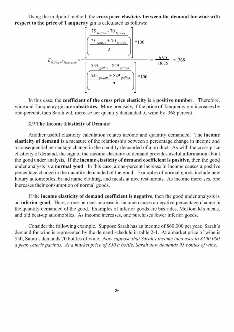
Using the midpoint method, the cross price elasticity between the demand for wine withrespect to the price of Tanqueray gin is calculated as follows:
In this case, the coefficient of the cross price elasticity is a positive number . Therefore,wine and Tanqueray gin are substitutes . More precisely, if the price of Tanqueray gin increases byone-percent, then Sarah will increase her quantity demanded of wine by .368 percent.
2.9 The Income Elasticity of Deman d
Another useful elasticity calculation relates income and quantity demanded. The incomeelasticity of demand is a measure of the relationship between a percentage change in income anda consequential percentage change in the quantity demanded of a product. As with the cross priceelasticity of demand, the sign of the income elasticity of demand provides useful information aboutthe good under analysis. If the income elasticity of demand coefficient is positive , then the goodunder analysis is a normal good . In this case, a one-percent increase in income causes a positive
percentage change in the quantity demanded of the good. Examples of normal goods include newluxury automobiles, brand name clothing, and meals at nice restaurants. As income increases, oneincreases their consumption of normal goods.
If the income elasticity of demand coefficient is negative , then the good under analysis isan inferior good . Here, a one-percent increase in income causes a negative percentage change inthe quantity demanded of the good. Examples of inferior goods are bus rides, McDonald’s meals,and old beat-up automobiles. As income increases, one purchases fewer inferior goods.
Consider the following example. Suppose Sarah has an income of $60,000 per year. Sarah’s
demand for wine is represented by the demand schedule in table 2-1. At a market price of wine is$50, Sarah’s demands 70 bottles of wine. Now suppose that Sarah’s income increases to $100,000a year, ceteris paribus. At a market price of $50 a bottle, Sarah now demands 95 bottles of wine.
75 bottles - 70 bottles
75 bottles + 70 bottles
2
*100
E QWine , P Tanqueray
=$35 gallon - $29 gallon
$35 gallon + $29 gallon
2
*100
= 6.9018.75
= .368
26
7/21/2019 PSU IVY Fundamentals of Economics
http://slidepdf.com/reader/full/psu-ivy-fundamentals-of-economics 29/118
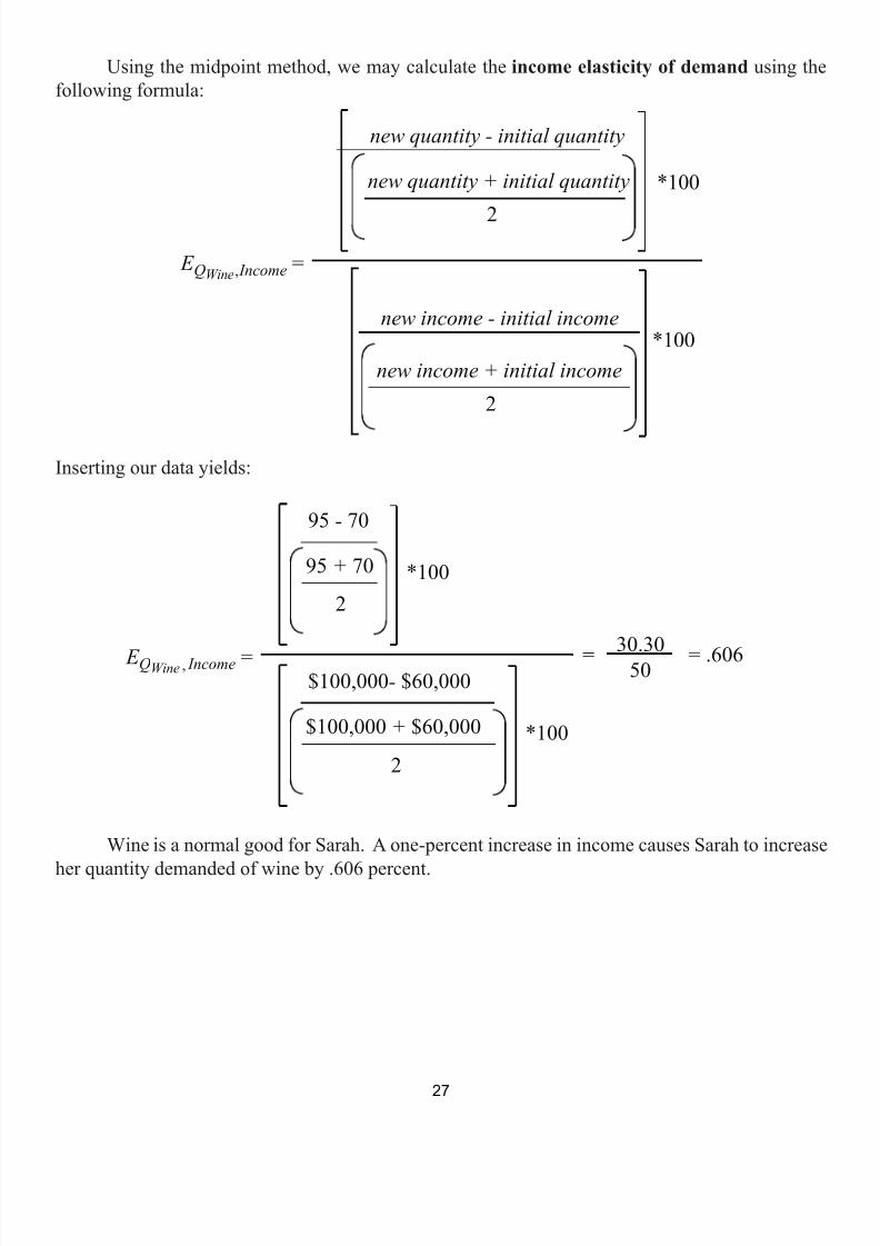
Using the midpoint method, we may calculate the income elasticity of demand using thefollowing formula:
Inserting our data yields:
Wine is a normal good for Sarah. A one-percent increase in income causes Sarah to increase
her quantity demanded of wine by .606 percent.
new quantity - initial quantity
new quantity + initial quantity
new income - initial income
new income + initial income2
2
*100
*100
E QWine , Income
=
95 - 70
95 + 70
2
*100
E QWine , Income =$100,000 - $60,000
$100,000 + $60,000
2
*100
= 30.30
50 = .606
,
,
27
7/21/2019 PSU IVY Fundamentals of Economics
http://slidepdf.com/reader/full/psu-ivy-fundamentals-of-economics 30/118
3. Supply
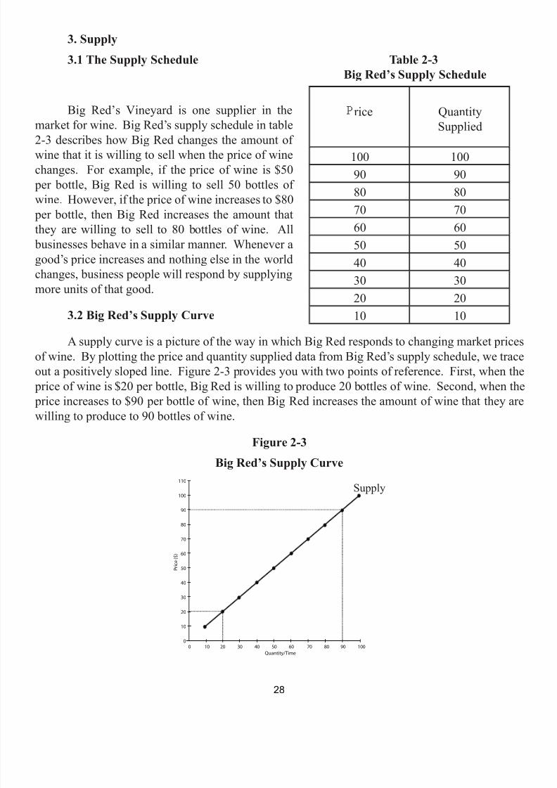
3.1 The Supply Schedule Table 2-3 Big Red’s Supply Schedule
Big Red’s Vineyard is one supplier in themarket for wine. Big Red’s supply schedule in table2-3 describes how Big Red changes the amount ofwine that it is willing to sell when the price of winechanges. For example, if the price of wine is $50
per bottle, Big Red is willing to sell 50 bottles ofwine. However, if the price of wine increases to $80
per bottle, then Big Red increases the amount thatthey are willing to sell to 80 bottles of wine. All
businesses behave in a similar manner. Whenever agood’s price increases and nothing else in the world
changes, business people will respond by supplyingmore units of that good.
3.2 Big Red’s Supply Curve
A supply curve is a picture of the way in which Big Red responds to changing market pricesof wine. By plotting the price and quantity supplied data from Big Red’s supply schedule, we traceout a positively sloped line. Figure 2-3 provides you with two points of reference. First, when the
price of wine is $20 per bottle, Big Red is willing to produce 20 bottles of wine. Second, when the price increases to $90 per bottle of wine, then Big Red increases the amount of wine that they arewilling to produce to 90 bottles of wine.
Figure 2-3
Big Red’s Supply Curve
rice QuantitySupplied
100 10090 9080 8070 7060 6050 5040 4030 3020 2010 10
�
��
�
�
�
�
�
�
�
�
�
�
�
�
Supply
28
7/21/2019 PSU IVY Fundamentals of Economics
http://slidepdf.com/reader/full/psu-ivy-fundamentals-of-economics 31/118
3.3 An Individual Supply Function
Big Red’s quantity supplied of wine is a dependent variable that depends on numerous in-dependent variables in addition to the market price of wine. Some of these independent variablesinclude the price of capital equipment (PCapita ), the rice of land (P Lan ), the price of labor (P La-
or ), the price of other inputs into the production process (P 1 … P ), the technology (TECH) used
by the organization, and the expectations (E) that the organization has with respect to the market.All of these variables may be succinctly expressed in the following general equation, where “g”signifies a general function.
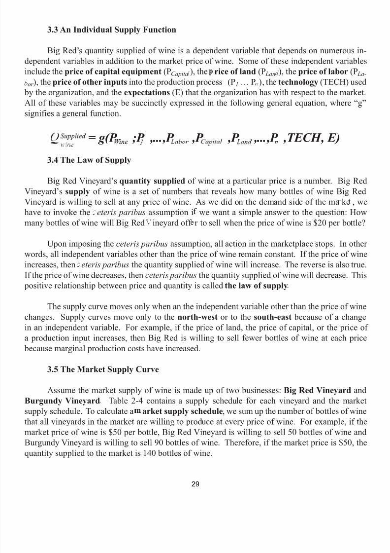
= g(P ;P ,...,P ,P ,P ,...,P ,TECH, E)
3.4 The Law of Supply
Big Red Vineyard’s quantity supplied of wine at a particular price is a number. Big Red
Vineyard’s supply of wine is a set of numbers that reveals how many bottles of wine Big RedVineyard is willing to sell at any price of wine. As we did on the demand side of the ma ke , wehave to invoke the eteris paribus assumption i we want a simple answer to the question: Howmany bottles of wine will Big Red ineyard off r to sell when the price of wine is $20 per bottle?
Upon imposing the ceteris paribus assumption, all action in the marketplace stops. In otherwords, all independent variables other than the price of wine remain constant. If the price of wineincreases, then eteris paribus the quantity supplied of wine will increase. The reverse is also true.If the price of wine decreases, then ceteris paribus the quantity supplied of wine will decrease. This
positive relationship between price and quantity is called the law of supply
The supply curve moves only when an the independent variable other than the price of winechanges. Supply curves move only to the north-west or to the south-east because of a changein an independent variable. For example, if the price of land, the price of capital, or the price ofa production input increases, then Big Red is willing to sell fewer bottles of wine at each price
because marginal production costs have increased.
3.5 The Market Supply Curve
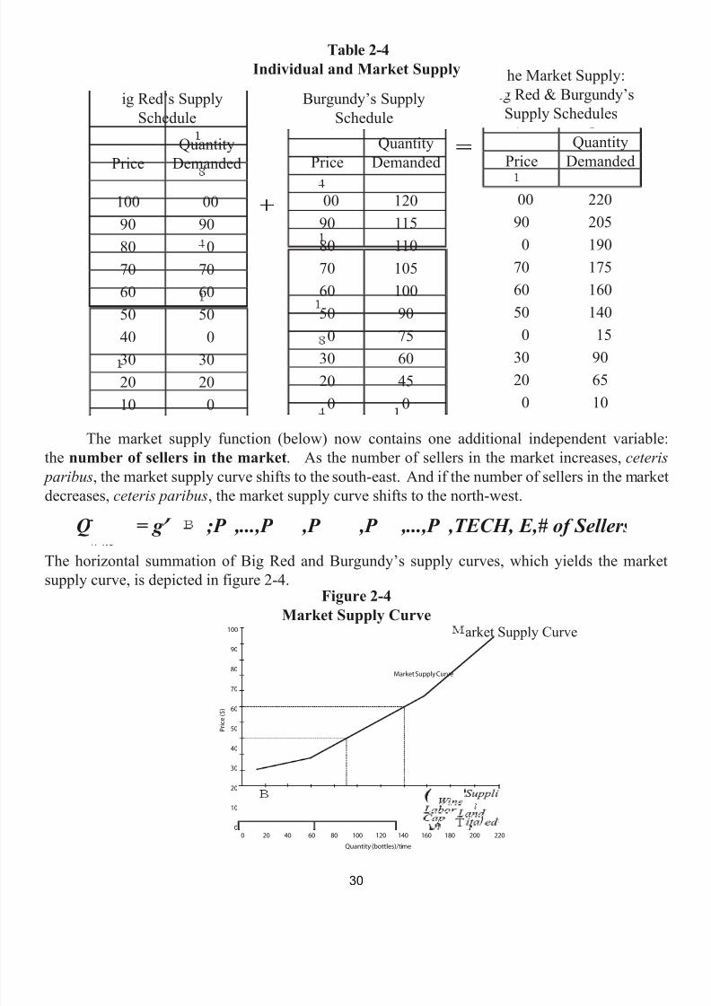
Assume the market supply of wine is made up of two businesses: Big Red Vineyard andBurgundy Vineyard Table 2-4 contains a supply schedule for each vineyard and the marketsupply schedule. To calculate a arket supply schedule , we sum up the number of bottles of winethat all vineyards in the market are willing to produce at every price of wine. For example, if themarket price of wine is $50 per bottle, Big Red Vineyard is willing to sell 50 bottles of wine andBurgundy Vineyard is willing to sell 90 bottles of wine. Therefore, if the market price is $50, thequantity supplied to the market is 140 bottles of wine.
29
7/21/2019 PSU IVY Fundamentals of Economics
http://slidepdf.com/reader/full/psu-ivy-fundamentals-of-economics 32/118
Table 2-4Individual and Market Supply
The market supply function (below) now contains one additional independent variable:the number of sellers in the market . As the number of sellers in the market increases, ceteris
paribus , the market supply curve shifts to the south-east. And if the number of sellers in the marketdecreases, ceteris paribus , the market supply curve shifts to the north-west.
Q = g P ;P ,...,P ,P ,P ,...,P ,TECH, E,# of SellersThe horizontal summation of Big Red and Burgundy’s supply curves, which yields the marketsupply curve, is depicted in figure 2-4.
Figure 2-4Market Supply Curve
PriceQuantity
Demanded
100 0090 9080 070 7060 6050 5040 030 3020 2010 0
PriceQuantity
Demanded
00 12090 11580 11070 10560 10050 90
0 7530 6020 45
0 0
PriceQuantity
Demanded
00 22090 205
0 19070 17560 16050 140
0 15
30 9020 65
0 10
ig Red’s SupplySchedule
Burgundy’s SupplySchedule
he Market Supply:ig Red & Burgundy’sSupply Schedules
w ne
��
�
�
�
�
�
�
�
�
�
�
�
�
arket Supply Curve
30

7/21/2019 PSU IVY Fundamentals of Economics
http://slidepdf.com/reader/full/psu-ivy-fundamentals-of-economics 33/118
3.6 The Supply Elasticity
The law of supply tells us that if the price of wine increases, eteris paribus, then the quantitydemanded of wine will increase. But by how much does it increase? The price elasticity of supplyhelps us answer this question. The price elasticity of supply is a measure of the relationship
between a percentage change in the market price of a product and a consequential percentage
change in the quantity supplied of a product.The following mid-point formula is what economists use to calculate the price elasticity of
supply.
The umerator contains the formula to calculate a percentage change in the quantity suppliedof wine The denominator contains the formula for calculating a ercentage change in the priceof the wine Dividing the percentage change in quantity supplied of wine by the percentage changein price of a wine, gives us the rice elasticity of supply or wine over the specified price range
Suppose the price of wine increases from $50 to $60 a bottle and as a result the quantitythat Burgundy is willing supply to the market increases from 90 bottles to 100 bottles. Using themid-point formula, we will now calculate Burgundy’s elasticity of supply over the $50 to $60 pricerange.
new quantity - initial quantity
new quantity + initial quantity
new price - initial price
new price + initial price2
2
*100
*100
eQWine , P Wine =
new quantity - initial quantity
new quantity + initial quantity
new price - initial price
new price + initial price2
2
eQWine , P Wine =
100 - 90
100 + 90
2
*100
$60 - $50
$60 + $50
2
*100
� �
10.53
18.18�
.579
,
,
31
7/21/2019 PSU IVY Fundamentals of Economics
http://slidepdf.com/reader/full/psu-ivy-fundamentals-of-economics 34/118
The coefficient of the supply elasticity is .579 for Burgundy Vineyard over the $50 to $60 price range. This coefficient tells us that if the price of wine increases by one-percent over this range,ceteris paribus , Burgundy Vineyard will increase their quantity supplied of wine by .579 percent.Because .579 is positive, the coefficient confirms our story that there exists a positive relationship
between changes in price and changes in the quantity supplied – this, of course, confirms the lawof supply.
4. Market Equilibrium
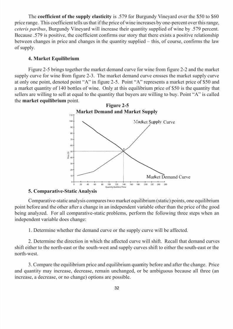
Figure 2-5 brings together the market demand curve for wine from figure 2-2 and the marketsupply curve for wine from figure 2-3. The market demand curve crosses the market supply curveat only one point, denoted point “A” in figure 2-5. Point “A” represents a market price of $50 anda market quantity of 140 bottles of wine. Only at this equilibrium price of $50 is the quantity thatsellers are willing to sell at equal to the quantity that buyers are willing to buy. Point “A” is calledthe market equilibrium point.
Figure 2-5Market Demand and Market Supply
5. Comparative-Static Analysis
Comparative-static analysis compares two market equilibrium (static) points, one equilibrium point before and the other after a change in an independent variable other than the price of the good being analyzed. For all comparative-static problems, perform the following three steps when anindependent variable does change:
1. Determine whether the demand curve or the supply curve will be affected.
2. Determine the direction in which the affected curve will shift. Recall that demand curvesshift either to the north-east or the south-west and supply curves shift to either the south-east or thenorth-west.
3. Compare the equilibrium price and equilibrium quantity before and after the change. Priceand quantity may increase, decrease, remain unchanged, or be ambiguous because all three (anincrease, a decrease, or no change) options are possible.
�
��
�
�
�
�
�
�
�
�
�
�
�
�
mand Curvear et De
Curver et Su
32
7/21/2019 PSU IVY Fundamentals of Economics
http://slidepdf.com/reader/full/psu-ivy-fundamentals-of-economics 35/118
5.1 A Shift in Demand 5.1.1 An Increase in the Price of a Substitute
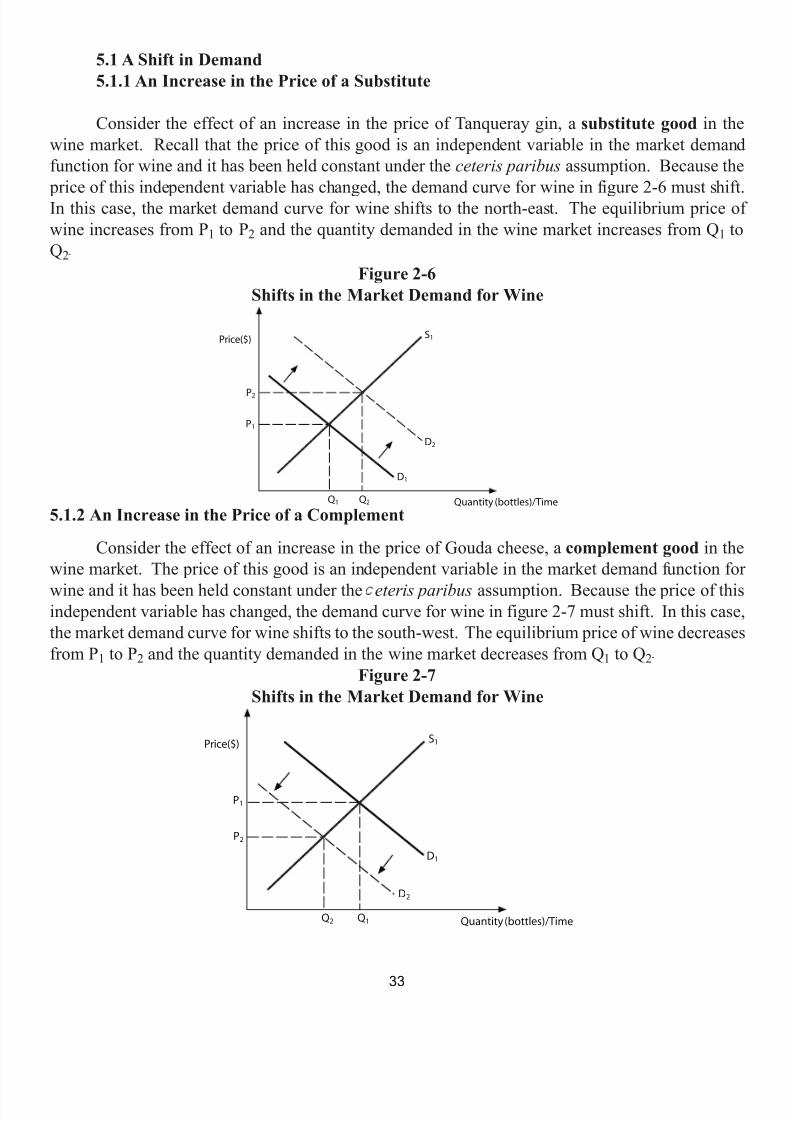
Consider the effect of an increase in the price of Tanqueray gin, a substitute good in thewine market. Recall that the price of this good is an independent variable in the market demandfunction for wine and it has been held constant under the ceteris paribus assumption. Because the
price of this independent variable has changed, the demand curve for wine in figure 2-6 must shift.In this case, the market demand curve for wine shifts to the north-east. The equilibrium price ofwine increases from P 1 to P 2 and the quantity demanded in the wine market increases from Q 1 toQ2
Figure 2-6Shifts in the Market Demand for Wine
5.1.2 An Increase in the Price of a Complement
Consider the effect of an increase in the price of Gouda cheese, a complement good in thewine market. The price of this good is an independent variable in the market demand function for
wine and it has been held constant under the eteris paribus assumption. Because the price of thisindependent variable has changed, the demand curve for wine in figure 2-7 must shift. In this case,the market demand curve for wine shifts to the south-west. The equilibrium price of wine decreasesfrom P 1 to P 2 and the quantity demanded in the wine market decreases from Q 1 to Q 2
Figure 2-7Shifts in the Market Demand for Wine
�
P1
Quantity (bottles)/Time
P2
Q1Q2
Price($)
D2
D1
S1
33

7/21/2019 PSU IVY Fundamentals of Economics
http://slidepdf.com/reader/full/psu-ivy-fundamentals-of-economics 36/118
5.1.3 A Decrease in Income for a Normal Good
Consider the effect of a decrease in income in the economy, and assume that wine is a normalgood . Section 2.3 defines a normal good. Income is an independent variable in the market demandfunction for wine and it has been held constant under the ceteris paribus assumption. Becauseincome has changed, the demand curve for wine in figure 2-8 must shift. In this case, the marketdemand curve for wine shifts to the south-west. The equilibrium price of wine decreases from P 1
to P2 and the quantity demanded in the wine market decreases from Q 1 to Q 2.
Figure 2-8Shifts in the Market Demand for Wine
5.1.4 A Decrease in Income for an Inferior Good
Consider the effect of a decrease in the income in the economy, and assume now that wine
is an inferior good . Section 2.3 defines an inferior good. Income is an independent variablein the market demand function for wine and it has been held constant under the ceteris paribusassumption. Because income has changed, the demand curve for wine in figure 2-9 must shift. Inthis case, the market demand curve for wine shifts to the north-east. The equilibrium price of wineincreases from P 1 to P 2 and the quantity demanded in the wine market increases from Q 1 to Q 2.
Figure 2-9Shifts in the Market Demand for Wine
P1
Quantity (bottles)/Time
P2
Q1Q2
Price($)
D2
D1
S1
�
34
7/21/2019 PSU IVY Fundamentals of Economics
http://slidepdf.com/reader/full/psu-ivy-fundamentals-of-economics 37/118
5.2 A Shift in Supply 5.2.1 An Increase in the Price of Labor
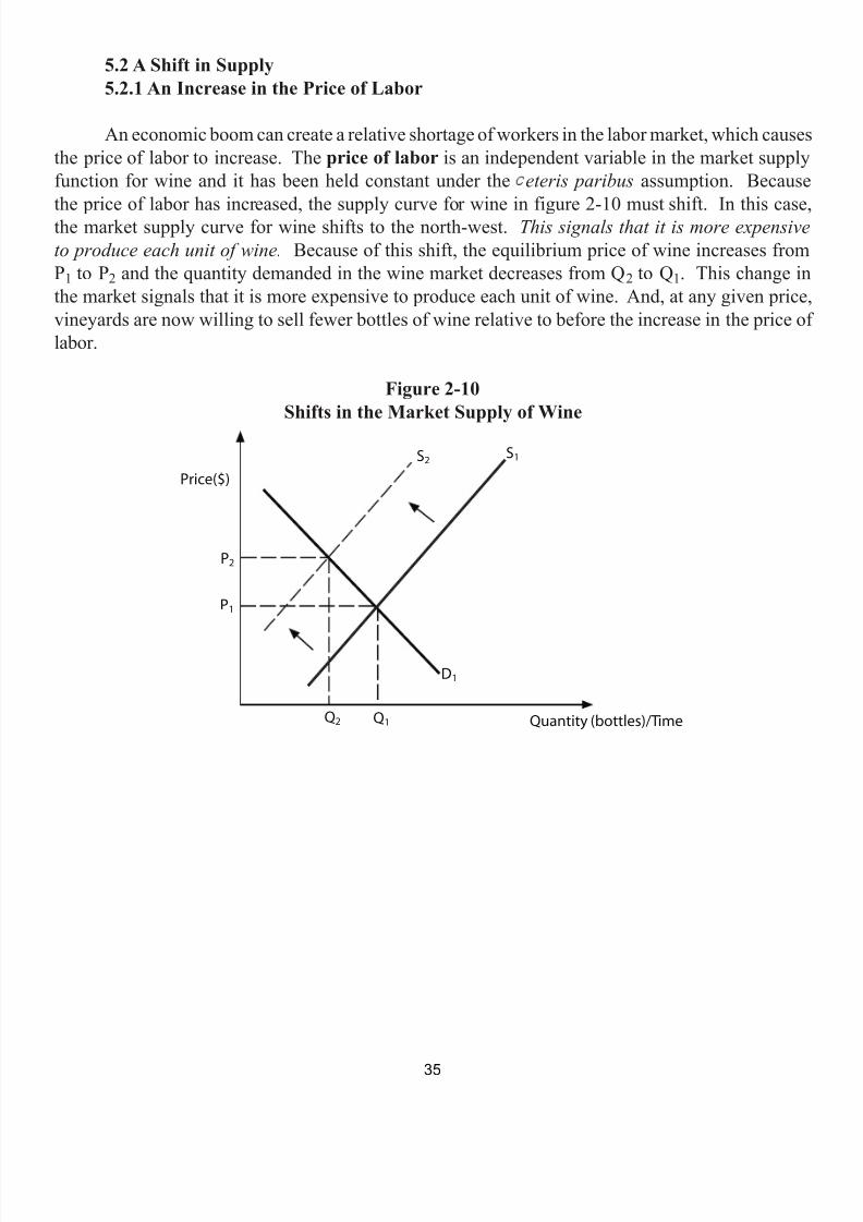
An economic boom can create a relative shortage of workers in the labor market, which causesthe price of labor to increase. The price of labor is an independent variable in the market supplyfunction for wine and it has been held constant under the eteris paribus assumption. Because
the price of labor has increased, the supply curve for wine in figure 2-10 must shift. In this case,the market supply curve for wine shifts to the north-west. This signals that it is more expensiveto produce each unit of wine. Because of this shift, the equilibrium price of wine increases fromP1 to P 2 and the quantity demanded in the wine market decreases from Q 2 to Q 1. This change inthe market signals that it is more expensive to produce each unit of wine. And, at any given price,vineyards are now willing to sell fewer bottles of wine relative to before the increase in the price oflabor.
Figure 2-10Shifts in the Market Supply of Wine
�
35
7/21/2019 PSU IVY Fundamentals of Economics
http://slidepdf.com/reader/full/psu-ivy-fundamentals-of-economics 38/118
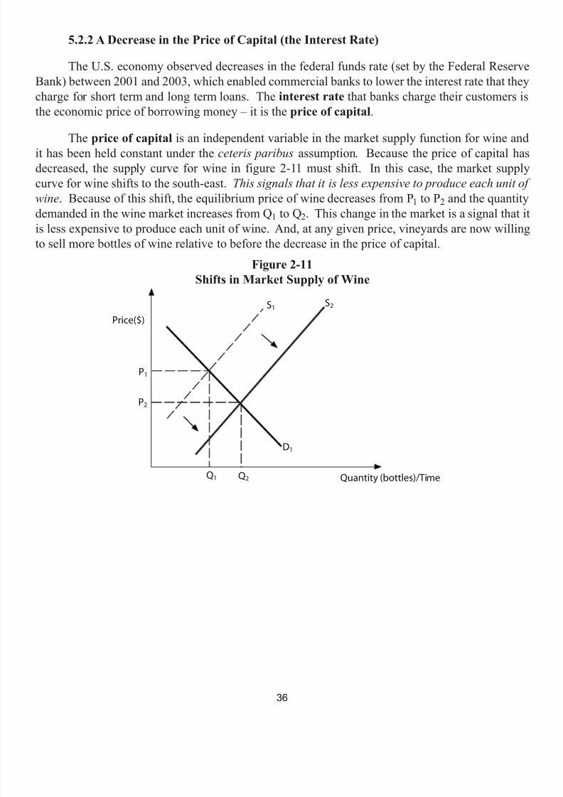
5.2.2 A Decrease in the Price of Capital (the Interest Rate)
The U.S. economy observed decreases in the federal funds rate (set by the Federal ReserveBank) between 2001 and 2003, which enabled commercial banks to lower the interest rate that theycharge for short term and long term loans. The interest rate that banks charge their customers isthe economic price of borrowing money – it is the price of capital .
The price of capital is an independent variable in the market supply function for wine andit has been held constant under the ceteris paribus assumption. Because the price of capital hasdecreased, the supply curve for wine in figure 2-11 must shift. In this case, the market supplycurve for wine shifts to the south-east. This signals that it is less expensive to produce each unit ofwine . Because of this shift, the equilibrium price of wine decreases from P 1 to P 2 and the quantitydemanded in the wine market increases from Q 1 to Q2. This change in the market is a signal that itis less expensive to produce each unit of wine. And, at any given price, vineyards are now willingto sell more bottles of wine relative to before the decrease in the price of capital.
Figure 2-11
Shifts in Market Supply of Wine
�
36
7/21/2019 PSU IVY Fundamentals of Economics
http://slidepdf.com/reader/full/psu-ivy-fundamentals-of-economics 39/118
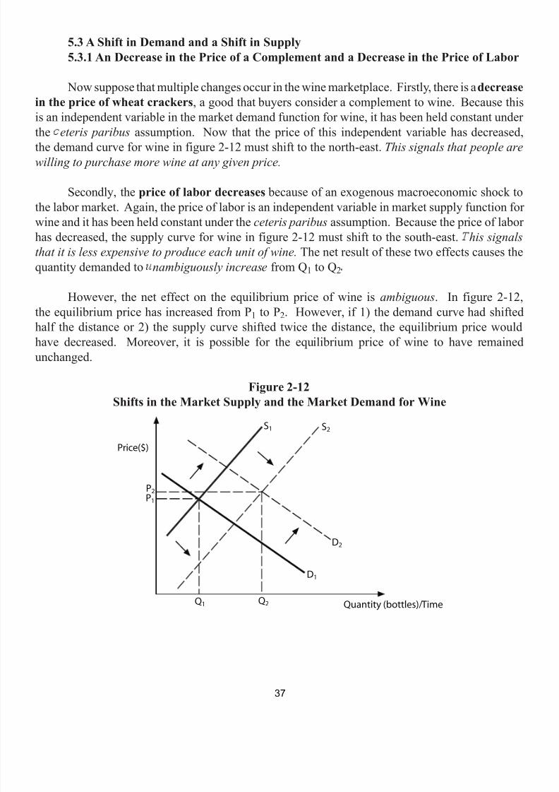
5.3 A Shift in Demand and a Shift in Supply 5.3.1 An Decrease in the Price of a Complement and a Decrease in the Price of Labor
Now suppose that multiple changes occur in the wine marketplace. Firstly, there is a decreasein the price of wheat crackers , a good that buyers consider a complement to wine. Because thisis an independent variable in the market demand function for wine, it has been held constant under
theeteris paribus
assumption. Now that the price of this independent variable has decreased,the demand curve for wine in figure 2-12 must shift to the north-east. This signals that people arewilling to purchase more wine at any given price.
Secondly, the price of labor decreases because of an exogenous macroeconomic shock tothe labor market. Again, the price of labor is an independent variable in market supply function forwine and it has been held constant under the ceteris paribus assumption. Because the price of laborhas decreased, the supply curve for wine in figure 2-12 must shift to the south-east. his signalsthat it is less expensive to produce each unit of wine. The net result of these two effects causes thequantity demanded to nambiguously increase from Q 1 to Q 2
However, the net effect on the equilibrium price of wine is ambiguous . In figure 2-12,the equilibrium price has increased from P 1 to P 2. However, if 1) the demand curve had shiftedhalf the distance or 2) the supply curve shifted twice the distance, the equilibrium price wouldhave decreased. Moreover, it is possible for the equilibrium price of wine to have remainedunchanged.
Figure 2-12Shifts in the Market Supply and the Market Demand for Wine
�
37

7/21/2019 PSU IVY Fundamentals of Economics
http://slidepdf.com/reader/full/psu-ivy-fundamentals-of-economics 40/118
5.3.2 An Increase in the Number of Buyers and an Increase in the Price of Land
Successful expenditures on advertising can have the effect of creating new buyers of wine.The number of buyers is an independent variable in the market demand function for wine, whichhas been held constant under the ceteris paribus assumption. With an increase in the number of
buyers, the demand curve for wine in figure 2-13 will shift to the north-east. This signals that more people are willing to purchase wine at any given price.
Second, suppose that there is a simultaneous increase in the price of land because all vineyardowners try to marginally increase their production capacity. The price of land is an independentvariable in market supply function for wine and it has been held constant under the ceteris paribusassumption. Because the price of land has increased, the market supply curve for wine in figure2-13 will shift to the north-west. The net result of these two effects causes the price of wine toincrease from P 1 to P 2.
However, the net effect on the equilibrium price is ambiguous . In figure 2-13, the equilibriumquantity has not changed. However, for example, if 1) the demand curve had shifted twice thedistance or 2) the supply curve shifted half the distance, the equilibrium quantity would haveincreased. Moreover, it is possible for the equilibrium quantity to have decreased if the demandshifted half the distance or supply curve shifted twice the distance shown in Figure 2-13. Thus,in this case, we would need additional information about the magnitude of the shifts for us todetermine the actual affect on the equilibrium quantity of wine.
Figure 2-13Shifts in the Market Supply and Market Demand for Wine
�
38

7/21/2019 PSU IVY Fundamentals of Economics
http://slidepdf.com/reader/full/psu-ivy-fundamentals-of-economics 41/118
5.4 Price Controls 5.4.1 A Binding Price Ceiling
A price ceiling is a government imposed and legally enforced maximum market price.Governments implement such policies with noble intentions. For example, government enforcedrent controls impose a maximum price for apartments, with the intention of increasing the number
of affordable apartments for lower income tenants. Nevertheless, the collective group of rentersand the market as a whole are never better off because of government imposed price ceilings ina market. Moreover, history has demonstrated that low income families have fewer apartmentsavailable to them when rent controls are in place.
Consider the wine market in figure 2-14. Before the price ceiling is imposed, the equilibrium price is $50 and the equilibrium quantity is Q 2 Now suppose the government imposes a priceceiling of $30 in the wine market. This means that $30 is the maximum price that any seller maycharge for a bottle of wine.
Figure 2-14A Binding Price Ceiling in the Wine Market
The $30 price ceiling is “ binding because the market price changes as a result of thegovernment policy. At a price ceiling of $30, the quantity demanded is Q 3 and the quantitysupplied at the price ceiling is Q 1. Because of the price ceiling, the quantity demandedexceeds the quantity supplied. There is a shortage of bottles of wine at the price ceiling.
The actual quantity sold in the market, however, equals Q 1. Therefore, the price ceilinghas actually reduced the number of bottles of wine bought and sold in the market by Q 2-Q1 It is
because of this, that we say that in the aggregate buyers and sellers are worse as a result of the $30 price ceiling.
Suppose, instead, the government imposed a price ceiling of $60 per bottle of wine. Inthis case, the maximum price that any seller may charge for a bottle of wine is $60. Becausethe equilibrium price is $50, the price ceiling is “ non-binding . The fact that the governmenthas declared that the price of wine cannot increase beyond $60 has no effect on this winemarket. The actual market price of wine remains in equilibrium at $50 per bottle. At theequilibrium price of $50, the quantity demand and the quantity supplied is Q 2. Thus, a non-
binding price ceiling has absolutely no effect on the equilibrium price or equilibrium quantity.
�
�
�
39

7/21/2019 PSU IVY Fundamentals of Economics
http://slidepdf.com/reader/full/psu-ivy-fundamentals-of-economics 42/118
5.4.2 A Binding Price Floor
A price floor is a government imposed and legally enforced minimum market price.Governments have implemented price floors with noble intentions, too. For example, the intentionof creating a living-wage for low income workers is a reason why policy-makers enact minimumwage legislation. Nevertheless, low-income workers, as a group, are never better off with aminimum wage. Some workers that are willing to work at a price below the minimum wage are nolonger offered a job after the minimum wage is imposed.
Consider the wine market in figure 2-15. Before the price floor is imposed, the equilibrium price is $50 and the equilibrium quantity is Q 2. Now suppose the government imposes a price floorof $70 in the wine market. This means that $70 is the minimum price that any seller may accept for
bottle of wine.Figure 2-15
A Binding Price Floor in the Wine Market
The $70 price floor is “ binding ” because the market price changes as a result of the government
policy. At a price floor of $70, the quantity demanded is Q 1 and the quantity supplied at the priceceiling is Q 3. Because of the price floor, the quantity supplied exceeds the quantity demanded.There is a surplus of wine being produced at the price floor.
The actual quantity sold in the market, however, equals Q 1. Therefore, the price floor hasactually reduced the number of bottles of wine sold in the market by Q 2-Q1. It is because of this,that we say that both the buyers and the sellers are worse off as a result of the $70 price ceiling.Collectively, the buyers buy fewer bottles of wine and the sellers sell fewer bottles of wine relativeto the volume of transactions before the price floor existed.
Suppose, instead, the government imposes a price floor of $30 per bottle of wine. In this case,the minimum price that any seller may charge for a bottle of wine is $30. Because the equilibrium
price is $50, the price floor is “ non-binding ”. The fact that the government has declared that price of wine cannot decrease below $30 has no effect on the wine market. The actual market priceremains in equilibrium at $50 per bottle. At the equilibrium price of $50, the quantity demandedand the quantity supplied equals Q 2. Thus, a non-binding price floor has absolutely no effect on theequilibrium price or equilibrium quantity.
�
�
�
40
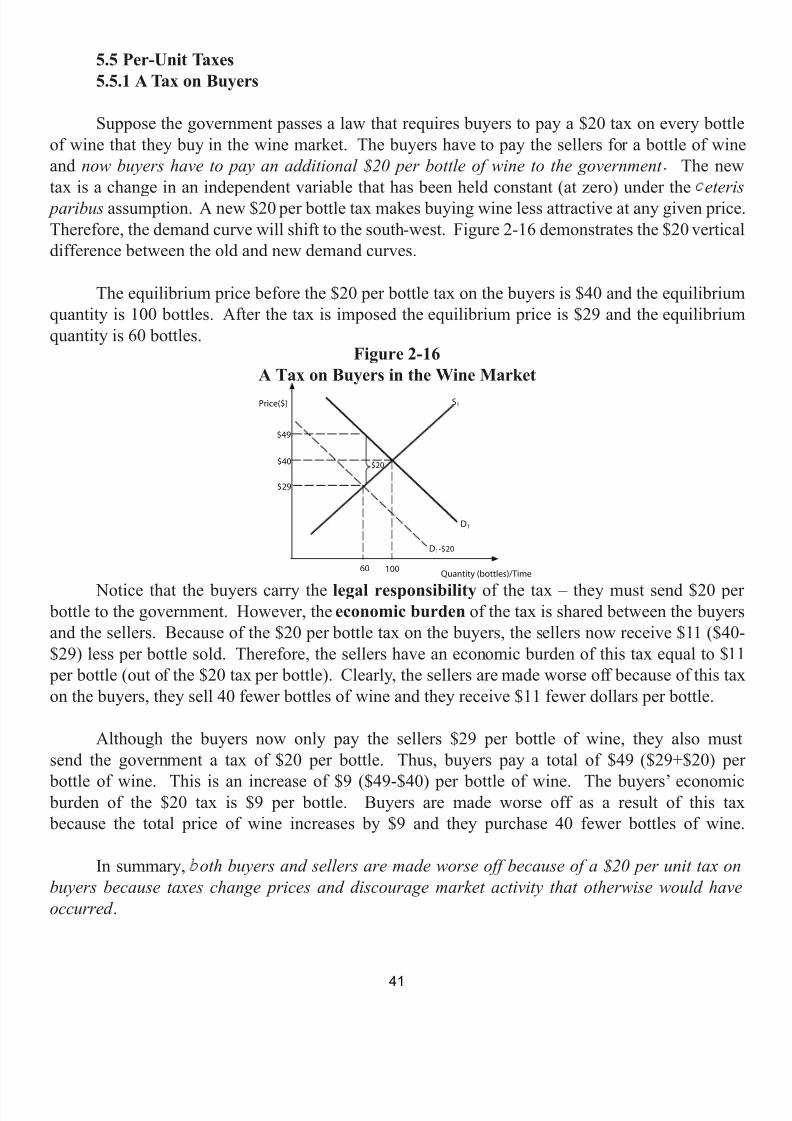
7/21/2019 PSU IVY Fundamentals of Economics
http://slidepdf.com/reader/full/psu-ivy-fundamentals-of-economics 43/118
5.5 Per-Unit Taxes 5.5.1 A Tax on Buyers
Suppose the government passes a law that requires buyers to pay a $20 tax on every bottleof wine that they buy in the wine market. The buyers have to pay the sellers for a bottle of wineand now buyers have to pay an additional $20 per bottle of wine to the government The new
tax is a change in an independent variable that has been held constant (at zero) under theeteris
paribus assumption. A new $20 per bottle tax makes buying wine less attractive at any given price.Therefore, the demand curve will shift to the south-west. Figure 2-16 demonstrates the $20 verticaldifference between the old and new demand curves.
The equilibrium price before the $20 per bottle tax on the buyers is $40 and the equilibriumquantity is 100 bottles. After the tax is imposed the equilibrium price is $29 and the equilibriumquantity is 60 bottles.
Figure 2-16A Tax on Buyers in the Wine Market
Notice that the buyers carry the legal responsibility of the tax – they must send $20 per bottle to the government. However, the economic burden of the tax is shared between the buyersand the sellers. Because of the $20 per bottle tax on the buyers, the sellers now receive $11 ($40-$29) less per bottle sold. Therefore, the sellers have an economic burden of this tax equal to $11
per bottle (out of the $20 tax per bottle). Clearly, the sellers are made worse off because of this taxon the buyers, they sell 40 fewer bottles of wine and they receive $11 fewer dollars per bottle.
Although the buyers now only pay the sellers $29 per bottle of wine, they also mustsend the government a tax of $20 per bottle. Thus, buyers pay a total of $49 ($29+$20) per
bottle of wine. This is an increase of $9 ($49-$40) per bottle of wine. The buyers’ economic burden of the $20 tax is $9 per bottle. Buyers are made worse off as a result of this tax because the total price of wine increases by $9 and they purchase 40 fewer bottles of wine.
In summary, oth buyers and sellers are made worse off because of a $20 per unit tax onbuyers because taxes change prices and discourage market activity that otherwise would haveoccurred .
�
�
�
�
��
41

7/21/2019 PSU IVY Fundamentals of Economics
http://slidepdf.com/reader/full/psu-ivy-fundamentals-of-economics 44/118
5.5.2 A Tax on Sellers
Suppose the government passes a law that requires sellers to pay a $20 tax on every bottleof wine that they sell in the wine market. Because the sellers have to pay the government $20 per
bottle of wine, the wine business becomes less profitable. Thus, the new tax will affect the marketsupply curve. The new tax is a change in an independent variable that has been held constant (atzero) under the ceteris paribus assumption. The $20 per bottle tax will cause the supply curve toshift to the north-west. Figure 2-17 demonstrates the $20 vertical difference between the old andnew supply curves.
The equilibrium price before the $20 per bottle tax on the sellers is $40 and the equilibriumquantity is 100 bottles. After the tax is imposed the equilibrium price is $49 and the equilibriumquantity is 60 bottles.
Figure 2-17A Tax on Sellers in the Wine Market
In this case, the sellers carry the legal responsibility of the tax – they must send $20 per bottle to the government. However, the economic burden of the tax is shared. The sellers nowreceive $49 from the buyers, of which they get to keep $29 ($49-$20) per bottle and they send thetax due of $20 per bottle to the government. The sellers have an economic burden of $11 ($40-$29)
per bottle (out of the $20 tax per bottle). The sellers are made worse off because of this tax; theysell 40 fewer bottles of wine and they get to keep $11 fewer dollars per bottle.
After the $20 tax on sellers is imposed, the buyers pay $49 per bottle of wine. This is anincrease of $9 ($49-$40) per bottle of wine. Thus, the buyers’ economic burden of the tax is $9($49-$40) per bottle (out of the $20 tax per bottle).
In summary, the economic burden of a $20 per bottle tax on buyers or a $20 per bottle tax on sellers is equivalent. Buyers and sellers are made worse off because of the $20 per unit tax. In botha tax on buyers and a tax on sellers, equilibrium quantity decreases by 40 bottles, the price paid bythe buyers increases by $9 per bottle, and the price that sellers keep decreases by $11 per bottle.
�
�
�
�
�
�
42
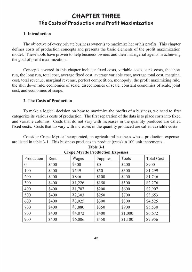
7/21/2019 PSU IVY Fundamentals of Economics
http://slidepdf.com/reader/full/psu-ivy-fundamentals-of-economics 45/118
CHAPTER THREEhe Costs of Production and Profit Maximization
1. Introduction
The objective of every private business owner is to maximize her or his profits. This chapterdefines costs of production concepts and presents the basic elements of the profit maximizationmodel. These tools have proven to help business owners and their managerial agents in achievingthe goal of profit maximization.
Concepts covered in this chapter include: fixed costs, variable costs, sunk costs, the shortrun, the long run, total cost, average fixed cost, average variable cost, average total cost, marginalcost, total revenue, marginal revenue, perfect competition, monopoly, the profit maximizing rule,the shut down rule, economies of scale, diseconomies of scale, constant economies of scale, jointcost, and economies of scope.
2. The Costs of Production
To make a logical decision on how to maximize the profits of a business, we need to firstcategorize its various costs of production. The first separation of the data is to place costs into fixedand variable columns. Costs that do not vary with increases in the quantity produced are calledfixed costs . Costs that do vary with increases in the quantity produced are called variable costs
Consider Crepe Myrtle Incorporated, an agricultural business whose production expenses
are listed in table 3-1. This business produces its product (trees) in 100 unit increments.Table 3-1Crepe Myrtle Production Expenses
Production Rent ages upplies ools Total Cost0 $400 300 $0 $200 $900100 $400 549 $50 $300 $1,299200 $400 846 $100 $400 $1,746300 $400 1,226 $150 $500 $2,276
400 $400 1,707 $200 $600 $2,907500 $400 2,303 $250 $700 $3,653600 $400 3,025 $300 $800 $4,525700 $400 3,880 $350 $900 $5,530800 $400 4,872 $400 $1,000 $6,672900 $400 6,006 $450 $1,100 $7,956
43
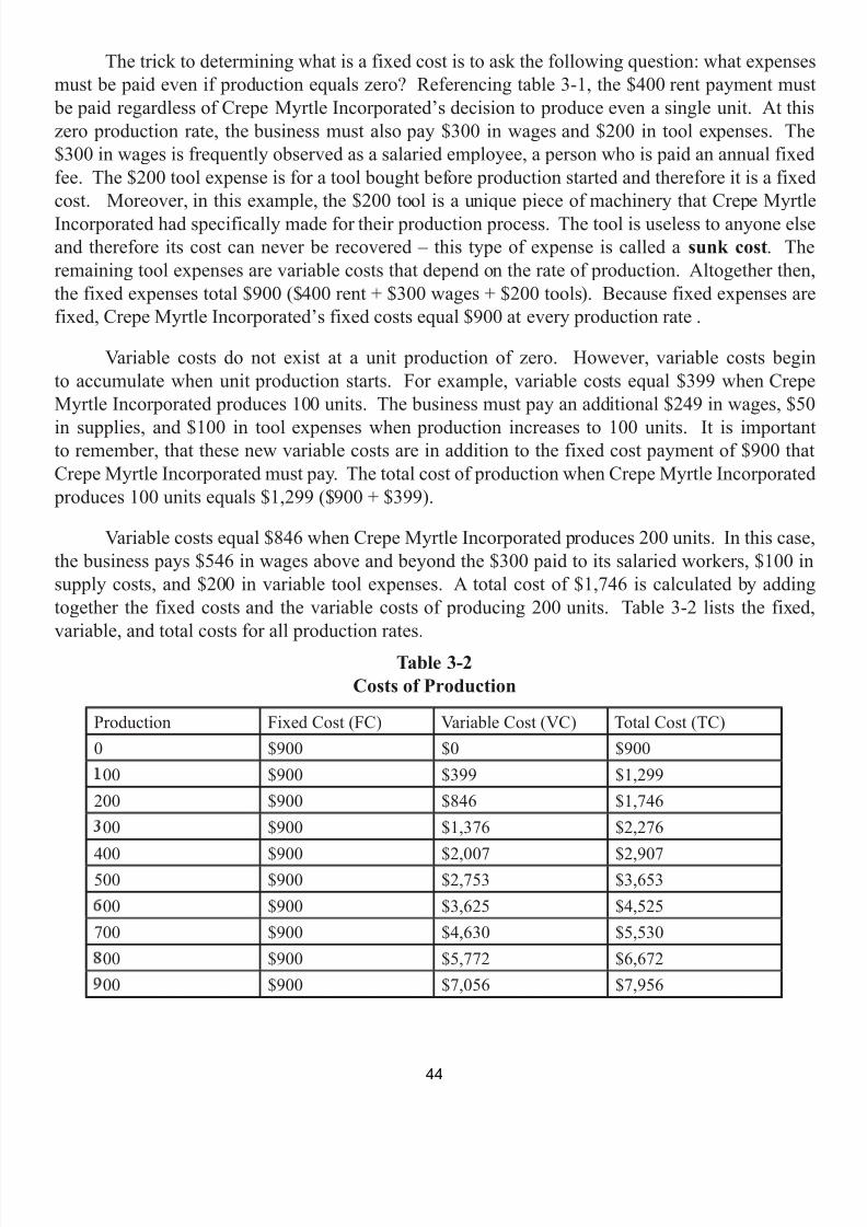
7/21/2019 PSU IVY Fundamentals of Economics
http://slidepdf.com/reader/full/psu-ivy-fundamentals-of-economics 46/118
The trick to determining what is a fixed cost is to ask the following question: what expensesmust be paid even if production equals zero? Referencing table 3-1, the $400 rent payment must
be paid regardless of Crepe Myrtle Incorporated’s decision to produce even a single unit. At thiszero production rate, the business must also pay $300 in wages and $200 in tool expenses. The$300 in wages is frequently observed as a salaried employee, a person who is paid an annual fixedfee. The $200 tool expense is for a tool bought before production started and therefore it is a fixedcost. Moreover, in this example, the $200 tool is a unique piece of machinery that Crepe MyrtleIncorporated had specifically made for their production process. The tool is useless to anyone elseand therefore its cost can never be recovered – this type of expense is called a sunk cost . Theremaining tool expenses are variable costs that depend on the rate of production. Altogether then,the fixed expenses total $900 ($400 rent + $300 wages + $200 tools). Because fixed expenses arefixed, Crepe Myrtle Incorporated’s fixed costs equal $900 at every production rate .
Variable costs do not exist at a unit production of zero. However, variable costs beginto accumulate when unit production starts. For example, variable costs equal $399 when CrepeMyrtle Incorporated produces 100 units. The business must pay an additional $249 in wages, $50
in supplies, and $100 in tool expenses when production increases to 100 units. It is importantto remember, that these new variable costs are in addition to the fixed cost payment of $900 thatCrepe Myrtle Incorporated must pay. The total cost of production when Crepe Myrtle Incorporated
produces 100 units equals $1,299 ($900 + $399).
Variable costs equal $846 when Crepe Myrtle Incorporated produces 200 units. In this case,the business pays $546 in wages above and beyond the $300 paid to its salaried workers, $100 insupply costs, and $200 in variable tool expenses. A total cost of $1,746 is calculated by addingtogether the fixed costs and the variable costs of producing 200 units. Table 3-2 lists the fixed,variable, and total costs for all production rates.
Table 3-2Costs of Production
Production Fixed Cost (FC) Variable Cost (VC) Total Cost (TC)0 $900 $0 $900
00 $900 $399 $1,299200 $900 $846 $1,746
00 $900 $1,376 $2,276
400 $900 $2,007 $2,907500 $900 $2,753 $3,653
00 $900 $3,625 $4,525700 $900 $4,630 $5,530
00 $900 $5,772 $6,67200 $900 $7,056 $7,956
44
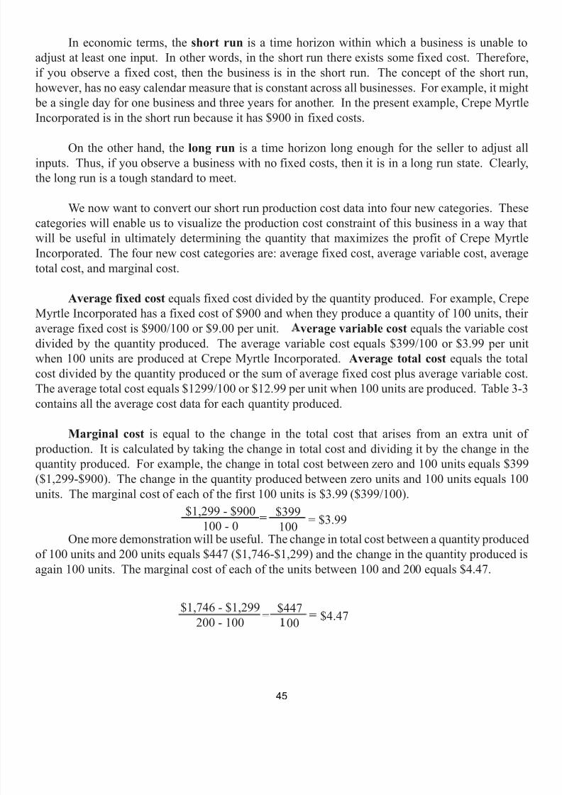
7/21/2019 PSU IVY Fundamentals of Economics
http://slidepdf.com/reader/full/psu-ivy-fundamentals-of-economics 47/118
In economic terms, the short run is a time horizon within which a business is unable toadjust at least one input. In other words, in the short run there exists some fixed cost. Therefore,if you observe a fixed cost, then the business is in the short run. The concept of the short run,however, has no easy calendar measure that is constant across all businesses. For example, it might
be a single day for one business and three years for another. In the present example, Crepe MyrtleIncorporated is in the short run because it has $900 in fixed costs.
On the other hand, the long run is a time horizon long enough for the seller to adjust allinputs. Thus, if you observe a business with no fixed costs, then it is in a long run state. Clearly,the long run is a tough standard to meet.
We now want to convert our short run production cost data into four new categories. Thesecategories will enable us to visualize the production cost constraint of this business in a way thatwill be useful in ultimately determining the quantity that maximizes the profit of Crepe MyrtleIncorporated. The four new cost categories are: average fixed cost, average variable cost, averagetotal cost, and marginal cost.
Average fixed cost equals fixed cost divided by the quantity produced. For example, CrepeMyrtle Incorporated has a fixed cost of $900 and when they produce a quantity of 100 units, theiraverage fixed cost is $900/100 or $9.00 per unit. verage variable cost equals the variable costdivided by the quantity produced. The average variable cost equals $399/100 or $3.99 per unitwhen 100 units are produced at Crepe Myrtle Incorporated. Average total cost equals the totalcost divided by the quantity produced or the sum of average fixed cost plus average variable cost.The average total cost equals $1299/100 or $12.99 per unit when 100 units are produced. Table 3-3contains all the average cost data for each quantity produced.
Marginal cost is equal to the change in the total cost that arises from an extra unit of production. It is calculated by taking the change in total cost and dividing it by the change in thequantity produced. For example, the change in total cost between zero and 100 units equals $399($1,299-$900). The change in the quantity produced between zero units and 100 units equals 100units. The marginal cost of each of the first 100 units is $3.99 ($399/100).
One more demonstration will be useful. The change in total cost between a quantity produced
of 100 units and 200 units equals $447 ($1,746-$1,299) and the change in the quantity produced isagain 100 units. The marginal cost of each of the units between 100 and 200 equals $4.47.
$1,299 - $900100 - 0
$399100 = $3.99
$1,746 - $1,299200 - 100
$44700= $4.47
45
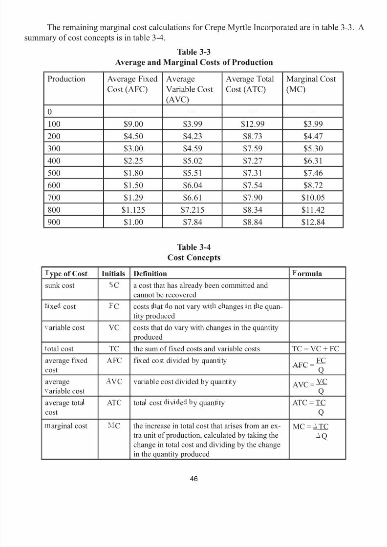
7/21/2019 PSU IVY Fundamentals of Economics
http://slidepdf.com/reader/full/psu-ivy-fundamentals-of-economics 48/118
The remaining marginal cost calculations for Crepe Myrtle Incorporated are in table 3-3. Asummary of cost concepts is in table 3-4.
Table 3-3Average and Marginal Costs of Production
Production Average FixedCost (AFC)
AverageVariable Cost(AVC)
Average TotalCost (ATC)
Marginal Cost(MC)
0100 $9.00 $3.99 $12.99 $3.99200 $4.50 $4.23 $8.73 $4.47300 $3.00 $4.59 $7.59 $5.30400 $2.25 $5.02 $7.27 $6.31500 $1.80 $5.51 $7.31 $7.46600 $1.50 $6.04 $7.54 $8.72700 $1.29 $6.61 $7.90 $10.05800 $1.125 $7.215 $8.34 $11.42900 $1.00 $7.84 $8.84 $12.84
Table 3-4Cost Concepts
ype of Cost Initials Definition ormula
sunk cost C a cost that has already been committed andcannot be recoveredxe cost C costs t at o not vary w t c anges n t e quan-
tity producedariable cost VC costs that do vary with changes in the quantity
producedotal cost TC the sum of fixed costs and variable costs TC = VC + FC
average fixedcost
AFC fixed cost divided by quantity AFC = FC Q
averageariable cost VC variable cost divided by quantity AVC = VC Qaverage totacost
ATC tota cost v e y quant ty ATC = TC Q
arginal cost C the increase in total cost that arises from an ex-tra unit of production, calculated by taking thechange in total cost and dividing by the changein the quantity produced
MC = TC Q
46
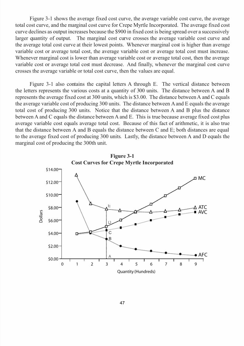
7/21/2019 PSU IVY Fundamentals of Economics
http://slidepdf.com/reader/full/psu-ivy-fundamentals-of-economics 49/118
Figure 3-1 shows the average fixed cost curve, the average variable cost curve, the averagetotal cost curve, and the marginal cost curve for Crepe Myrtle Incorporated. The average fixed costcurve declines as output increases because the $900 in fixed cost is being spread over a successivelylarger quantity of output. The marginal cost curve crosses the average variable cost curve andthe average total cost curve at their lowest points. Whenever marginal cost is higher than averagevariable cost or average total cost, the average variable cost or average total cost must increase.
Whenever marginal cost is lower than average variable cost or average total cost, then the averagevariable cost or average total cost must decrease. And finally, whenever the marginal cost curvecrosses the average variable or total cost curve, then the values are equal.
Figure 3-1 also contains the capital letters A through E. The vertical distance betweenthe letters represents the various costs at a quantity of 300 units. The distance between A and Brepresents the average fixed cost at 300 units, which is $3.00. The distance between A and C equalsthe average variable cost of producing 300 units. The distance between A and E equals the averagetotal cost of producing 300 units. Notice that the distance between A and B plus the distance
between A and C equals the distance between A and E. This is true because average fixed cost plusaverage variable cost equals average total cost. Because of this fact of arithmetic, it is also truethat the distance between A and B equals the distance between C and E; both distances are equalto the average fixed cost of producing 300 units. Lastly, the distance between A and D equals themarginal cost of producing the 300th unit.
Figure 3-1Cost Curves for Crepe Myrtle Incorporated
�
�
�
�
�
�
�
�
�
�
C
B
47
7/21/2019 PSU IVY Fundamentals of Economics
http://slidepdf.com/reader/full/psu-ivy-fundamentals-of-economics 50/118
3. The Profit Maximizing Decision
The last few pages have organized Crepe Myrtle Incorporated’s expense statement intocategories that economists find helpful in the ultimate task of discovering where the businessmaximizes its profits. The next step is to analyze the revenue constraint of the business. In thefirst case below, we assume that Crepe Myrtle Incorporated is one of many perfectly competitive
businesses in the Crepe Myrtle tree industry. In the second case, we assume that Crepe MyrtleIncorporated is a monopoly.
3.1 Application: Profit maximizing in a Perfectly Competitive Industry
There are three characteristics of a perfectly competitive industry:
• there are many buyers and sellers,• the good is homogeneous (e.g., trees or peas), and• all who want to enter the industry are free to do so and any business may exit at a
time of their choosing.
These conditions that define a perfectly competitive industry imply that no business mayinfluence the market price of the product that they sell. It is because of this that businesses operatingin perfectly competitive industries are said to be price takers .
In a perfectly competitive industry, market prices are determined by the interaction of themarket demand and market supply curves. Consider the case where the Crepe Myrtle tree market
price equals $10.05 per unit. Because Crepe Myrtle Incorporated is one of many businesses in the
Crepe Myrtle Market, it must charge $10.05 per unit. To set any higher price would devastate the business because zero units would be sold. Customers would simply purchase their Crepe Myrtletrees from other businesses that are charging the lower market price of $10.05.
Total revenue and marginal revenue data for Crepe Myrtle Incorporated when the market price is $10.05 per unit are in table 3-5. Total revenue is calculated by multiplying price andquantity. For example, if quantity is 300 units, then total revenue equals $3,015.
_______________________ Perfect competition does not occur frequently in the real world. Competition in many industries is so
fierce that the model of perfect competition is of enormous help in predicting the behavior of the firms inthese industries. Farming, fishing, grocery retailing, plumbing, and dry cleaning are all good examples ofn ustr es t at are g y compet t ve.
48
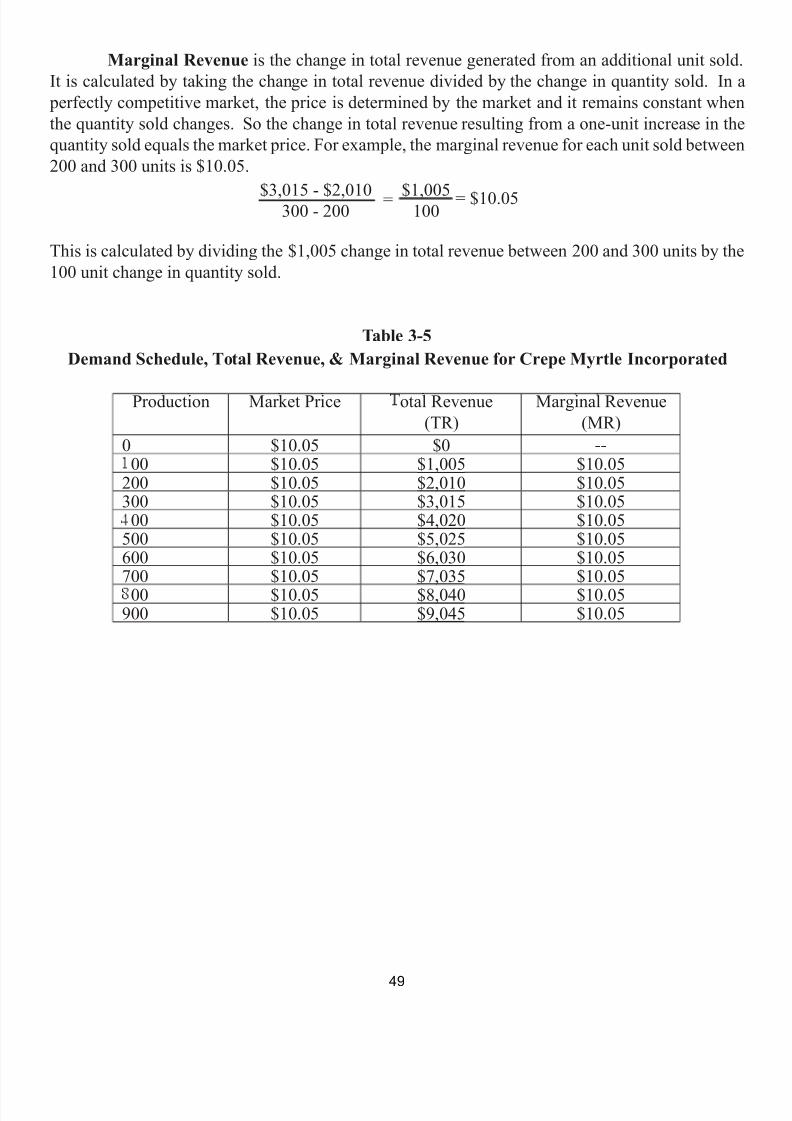
7/21/2019 PSU IVY Fundamentals of Economics
http://slidepdf.com/reader/full/psu-ivy-fundamentals-of-economics 51/118
Marginal Revenue is the change in total revenue generated from an additional unit sold.It is calculated by taking the change in total revenue divided by the change in quantity sold. In a
perfectly competitive market, the price is determined by the market and it remains constant whenthe quantity sold changes. So the change in total revenue resulting from a one-unit increase in thequantity sold equals the market price. For example, the marginal revenue for each unit sold between200 and 300 units is $10.05.
This is calculated by dividing the $1,005 change in total revenue between 200 and 300 units by the100 unit change in quantity sold.
Table 3-5Demand Schedule, Total Revenue, & Marginal Revenue for Crepe Myrtle Incorporated
Production Market Price otal Revenue(TR)
Marginal Revenue(MR)
0 $10.05 $000 $10.05 $1,005 $10.05
200 $10.05 $2,010 $10.05300 $10.05 $3,015 $10.05
00 $10.05 $4,020 $10.05500 $10.05 $5,025 $10.05600 $10.05 $6,030 $10.05700 $10.05 $7,035 $10.05
00 $10.05 $8,040 $10.05900 $10.05 $9,045 $10.05
$3,015 - $2,010300 - 200 $1,005100 = $10.05=
49

7/21/2019 PSU IVY Fundamentals of Economics
http://slidepdf.com/reader/full/psu-ivy-fundamentals-of-economics 52/118
In the pursuit of maximizing profits, business owners are constrained in two fundamentalways. Firstly, the competency of its employees and the market prices of inputs into the production
process dictate the costs of producing output, i.e., competencies and input prices determine the datain table 3-2 and table 3-3. Secondly, the price that a perfectly competitive business can charge isdetermined by the market, and not the business owner.
Given these two constraints the business owner’s key task is to make two decisions.
• The first decision is to determine the profit maximizing quantity to produce.
• In the short run, the second decision is to decide whether to produce or to shut down the business for a short period of time.
• In the long run, the second decision is to decide whether to produce or to exi the industry,forever.
Let’s walk through an example. Consider Crepe Myrtle Incorporated’s marginal cost datafrom table 3-2 and the marginal revenue data from table 3-5, both of which are graphed in figure3-2.
50
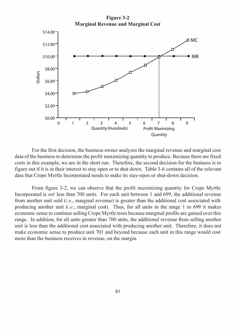
7/21/2019 PSU IVY Fundamentals of Economics
http://slidepdf.com/reader/full/psu-ivy-fundamentals-of-economics 53/118
Figure 3-2arginal Revenue and Marginal Cost
For the first decision, the business owner analyzes the marginal revenue and marginal costdata of the business to determine the profit maximizing quantity to produce. Because there are fixedcosts in this example, we are in the short run. Therefore, the second decision for the business is tofigure out if it is in their interest to stay open or to shut down. Table 3-6 contains all of the relevant
data that Crepe Myrtle Incorporated needs to make its stay-open or shut-down decision.
From figure 3-2, we can observe that the profit maximizing quantity for Crepe MyrtleIncorporated is no less than 700 units. For each unit between 1 and 699, the additional revenuefrom another unit sold ( .e., marginal revenue) is greater than the additional cost associated with
producing another unit ( .e., marginal cost). Thus, for all units in the range 1 to 699 it makeseconomic sense to continue selling Crepe Myrtle trees because marginal profits are gained over thisrange. In addition, for all units greater than 700 units, the additional revenue from selling anotherunit is less than the additional cost associated with producing another unit. Therefore, it does not
make economic sense to produce unit 701 and beyond because each unit in this range would costmore than the business receives in revenue, on the margin.
�
�
�
�
�
�
�
�
�
�
51

7/21/2019 PSU IVY Fundamentals of Economics
http://slidepdf.com/reader/full/psu-ivy-fundamentals-of-economics 54/118
The incentive to increase profits over the 1-699 range and the fear of losing profits over the701+ range leads us to our optimal profit maximizing quantity: 700 units. The additional revenuereceived by selling the 700 unit is $10.05 and the additional cost incurred because of producingthe 700 th unit is $10.05. At the 700 th unit marginal revenue equals marginal cost. This result issummarized in what economists call the profit maximizing rule he profit maximizing rule
states that a business maximizes profits when it produces where the marginal revenue from sellinganother unit equals the marginal cost of producing an additional unit
Using Crepe Myrtle Incorporated’s marginal revenue and marginal cost data and the profitmaximizing rule, we’ve concluded that 700 units is the optimal quantity to produce. At that quantity,table 3-6 reports that total revenue equals $7,035 and total cost equals $5,530. In the short run, the
business is making a positive economic profit and it should stay open and produce 700 units.Table 3-6
Crepe Myrtle Incorporated’s Revenue and Cost Data
roduction Marginalevenue (MR)
MarginalCost(MC)
Total Revenue(TR)
Total Cost(TC)
Profit( )
0 $0 $900 -$90000 $10.05 $3.99 $1,005 $1,299 -$294
200 $10.05 $4.47 $2,010 $1,746 $264300 $10.05 $5.30 $3,015 $2,276 $739
00 $10.05 $6.31 $4,020 $2,907 $1,113500 $10.05 $7.46 $5,025 $3,653 $1,372600 $10.05 $8.72 $6,030 $4,525 $1,505700 $10.05 $10.05 $7,035 $5,530 $1,505
00 $10.05 $11.42 $8,040 $6,672 $1,368900 $10.05 $12.84 $9,045 $7,956 $1,089
Suppose something happens in the Crepe Myrtle market and the market price drops to$5.30 per Crepe Myrtle tree. How should Crepe Myrtle Incorporated respond to this change ineconomic events?
First, they must find there new profit maximizing quantity. Second, they must make anothershut-down or stay-open decision. Table 3-7 contains the new revenue data for a market price of$5.30 in addition to the previous cost of production data, which has not changed.
___________________ The business is actually indifferent at this point, but for analytical ease we adopt a policy of: if indifferent,
produce it.
52
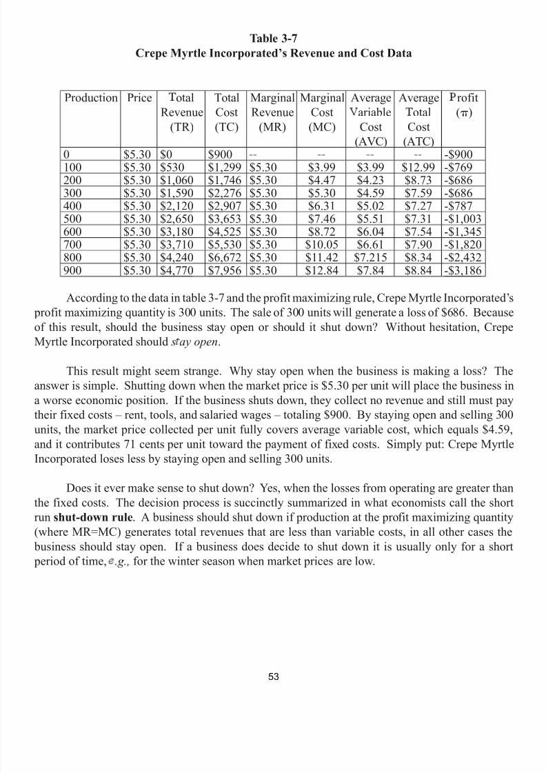
7/21/2019 PSU IVY Fundamentals of Economics
http://slidepdf.com/reader/full/psu-ivy-fundamentals-of-economics 55/118
Table 3-7Crepe Myrtle Incorporated’s Revenue and Cost Data
Production Price otalRevenue
(TR)
TotalCost(TC)
MarginalRevenue
(MR)
MarginalCost(MC)
AverageariableCost
(AVC)
Averageotal
Cost(ATC)
rofit(p )
0 $5.30 $0 $900 -$900100 $5.30 $530 $1,299 $5.30 $3.99 $3.99 $12.99 -$769200 $5.30 $1,060 $1,746 $5.30 $4.47 $4.23 $8.73 -$686300 $5.30 $1,590 $2,276 $5.30 $5.30 $4.59 $7.59 -$686400 $5.30 $2,120 $2,907 $5.30 $6.31 $5.02 $7.27 -$787500 $5.30 $2,650 $3,653 $5.30 $7.46 $5.51 $7.31 -$1,003600 $5.30 $3,180 $4,525 $5.30 $8.72 $6.04 $7.54 -$1,345700 $5.30 $3,710 $5,530 $5.30 $10.05 $6.61 $7.90 -$1,820800 $5.30 $4,240 $6,672 $5.30 $11.42 $7.215 $8.34 -$2,432900 $5.30 $4,770 $7,956 $5.30 $12.84 $7.84 $8.84 -$3,186
According to the data in table 3-7 and the profit maximizing rule, Crepe Myrtle Incorporated’s profit maximizing quantity is 300 units. The sale of 300 units will generate a loss of $686. Becauseof this result, should the business stay open or should it shut down? Without hesitation, CrepeMyrtle Incorporated should s ay open .
This result might seem strange. Why stay open when the business is making a loss? Theanswer is simple. Shutting down when the market price is $5.30 per unit will place the business in
a worse economic position. If the business shuts down, they collect no revenue and still must paytheir fixed costs – rent, tools, and salaried wages – totaling $900. By staying open and selling 300units, the market price collected per unit fully covers average variable cost, which equals $4.59,and it contributes 71 cents per unit toward the payment of fixed costs. Simply put: Crepe MyrtleIncorporated loses less by staying open and selling 300 units.
Does it ever make sense to shut down? Yes, when the losses from operating are greater thanthe fixed costs. The decision process is succinctly summarized in what economists call the shortrun shut-down rule . A business should shut down if production at the profit maximizing quantity(where MR=MC) generates total revenues that are less than variable costs, in all other cases the
business should stay open. If a business does decide to shut down it is usually only for a short period of time, .g., for the winter season when market prices are low.
53
7/21/2019 PSU IVY Fundamentals of Economics
http://slidepdf.com/reader/full/psu-ivy-fundamentals-of-economics 56/118
When prices remain low for very long periods of time, then the business moves into a longrun decision mode. In the long run, there are no fixed costs. A business must decide to stay open orexit the industry in the long run. The ong run exit decision states that a business should exit theindustry if production at the profit maximizing quantity (where MR=MC) generates total revenuesthat are less than total cost, otherwise stay open.
3.2 Application: Profit Maximizing and a Monopolistic Industry
Three characteristics define a monopolistic industry. In this type of industry:
• there are many buyers and only one seller,• the good is heterogeneous (e.g., Microsoft Office is different from other software
applications), and• barriers to entering the market exist (e.g., patents are barriers that make it illegal
or someone to produce a product without permission of the patent owner).
In a monopolistic industry, because there is only one seller of a product the business owneractually goes through a process of setting the price of its product, a task that competitive firms areunable to do. Thus monopolistic firms are called rice setters
Assume Crepe Myrtle Incorporated is now a monopoly. The business faces the entiremarket demand for its product because it is now the only business that sells Crepe Myrtle trees.Consider the market demand data listed in table 3-8 (the first two columns show the market demandschedule). If the business produces 100 units, it can sell them at $16.02 each. If it produces 200
units, then it must lower the price to $14.93 in order to sell all 200 units. If it produces 300 units,then it must lower the price to $13.88 in order to sell all 300 units. And so on. The two columnsreveal a downward sloping demand curve, which is shown in figure 3-3.
Total revenue and marginal revenue for Crepe Myrtle Incorporated is in table 3-8. Totalrevenue is calculated by multiplying price and quantity. For example, if the quantity is 300 units,then total revenue equals $4,164 ($13.88 x 300).
Marginal Revenue is the change in total revenue from an additional unit sold. It is calculated
by taking the change in total revenue divided by the change in quantity sold. For example, themarginal revenue for each unit sold between 200 and 300 units is $11.78. This is calculated bydividing $1,178, the change in total revenue between 200 and 300 units, by 100, the change inquantity sold between 200 and 300 units. The marginal revenue schedule is listed in table 3.8 andgraphed in figure 3-3.
54
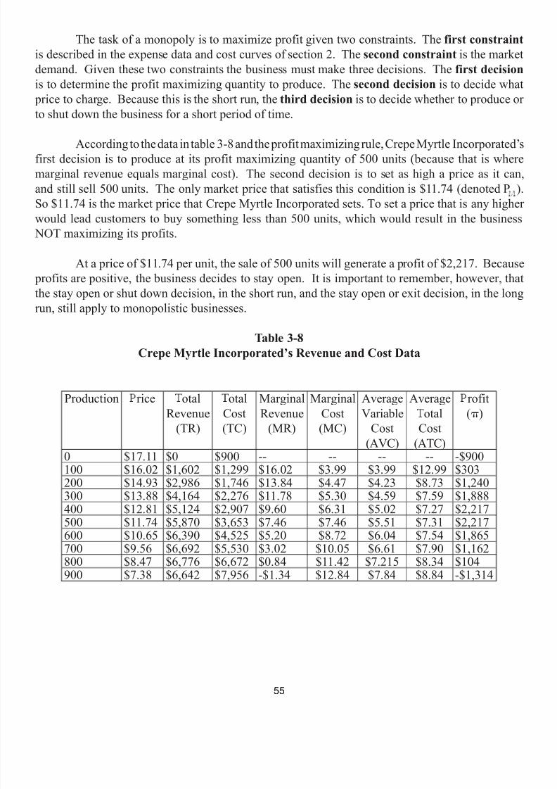
7/21/2019 PSU IVY Fundamentals of Economics
http://slidepdf.com/reader/full/psu-ivy-fundamentals-of-economics 57/118
The task of a monopoly is to maximize profit given two constraints. The first constraintis described in the expense data and cost curves of section 2. The second constraint is the marketdemand. Given these two constraints the business must make three decisions. The first decisionis to determine the profit maximizing quantity to produce. The second decision is to decide what
price to charge. Because this is the short run, the third decision is to decide whether to produce orto shut down the business for a short period of time.
According to the data in table 3-8 and the profit maximizing rule, Crepe Myrtle Incorporated’sfirst decision is to produce at its profit maximizing quantity of 500 units (because that is wheremarginal revenue equals marginal cost). The second decision is to set as high a price as it can,and still sell 500 units. The only market price that satisfies this condition is $11.74 (denoted P ).So $11.74 is the market price that Crepe Myrtle Incorporated sets. To set a price that is any higherwould lead customers to buy something less than 500 units, which would result in the business
NOT maximizing its profits.
At a price of $11.74 per unit, the sale of 500 units will generate a profit of $2,217. Because profits are positive, the business decides to stay open. It is important to remember, however, thatthe stay open or shut down decision, in the short run, and the stay open or exit decision, in the longrun, still apply to monopolistic businesses.
Table 3-8Crepe Myrtle Incorporated’s Revenue and Cost Data
Production rice otal
Revenue(TR)
otal
Cost(TC)
Marginal
Revenue(MR)
Marginal
Cost(MC)
Average
VariableCost
(AVC)
Average
otalCost
(ATC)
rofit
(p )
0 $17.11 $0 $900 -- -- -- -- -$900100 $16.02 $1,602 $1,299 $16.02 $3.99 $3.99 $12.99 $303200 $14.93 $2,986 $1,746 $13.84 $4.47 $4.23 $8.73 $1,240300 $13.88 $4,164 $2,276 $11.78 $5.30 $4.59 $7.59 $1,888400 $12.81 $5,124 $2,907 $9.60 $6.31 $5.02 $7.27 $2,217500 $11.74 $5,870 $3,653 $7.46 $7.46 $5.51 $7.31 $2,217600 $10.65 $6,390 $4,525 $5.20 $8.72 $6.04 $7.54 $1,865
700 $9.56 $6,692 $5,530 $3.02 $10.05 $6.61 $7.90 $1,162800 $8.47 $6,776 $6,672 $0.84 $11.42 $7.215 $8.34 $104900 $7.38 $6,642 $7,956 -$1.34 $12.84 $7.84 $8.84 -$1,314
55
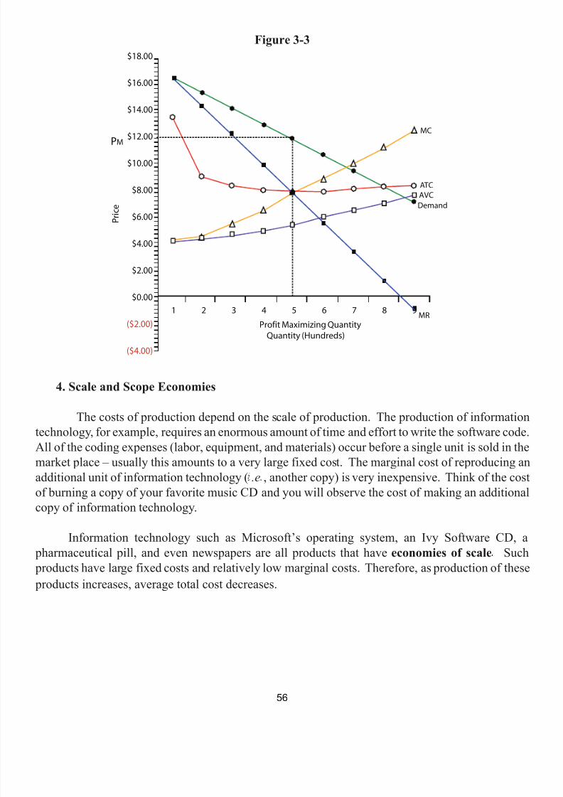
7/21/2019 PSU IVY Fundamentals of Economics
http://slidepdf.com/reader/full/psu-ivy-fundamentals-of-economics 58/118
Figure 3-3
4. Scale and Scope Economies
The costs of production depend on the scale of production. The production of informationtechnology, for example, requires an enormous amount of time and effort to write the software code.All of the coding expenses (labor, equipment, and materials) occur before a single unit is sold in themarket place – usually this amounts to a very large fixed cost. The marginal cost of reproducing anadditional unit of information technology ( .e , another copy) is very inexpensive. Think of the costof burning a copy of your favorite music CD and you will observe the cost of making an additionalcopy of information technology.
Information technology such as Microsoft’s operating system, an Ivy Software CD, a
pharmaceutical pill, and even newspapers are all products that have economies of scale Such products have large fixed costs and relatively low marginal costs. Therefore, as production of these products increases, average total cost decreases.
�
�
�
�
�
�
�
�
�
�
�
�
�
�
56
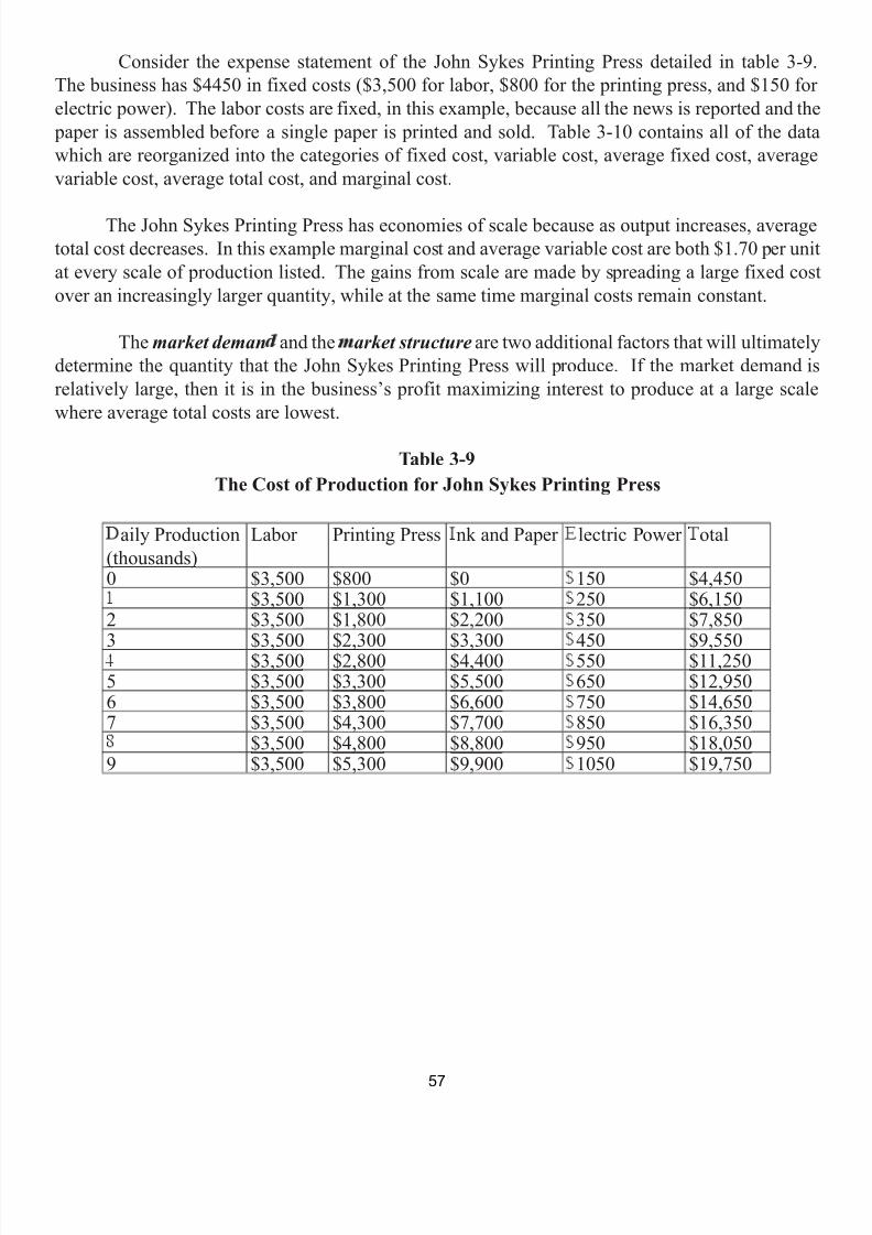
7/21/2019 PSU IVY Fundamentals of Economics
http://slidepdf.com/reader/full/psu-ivy-fundamentals-of-economics 59/118
Consider the expense statement of the John Sykes Printing Press detailed in table 3-9.The business has $4450 in fixed costs ($3,500 for labor, $800 for the printing press, and $150 forelectric power). The labor costs are fixed, in this example, because all the news is reported and the
paper is assembled before a single paper is printed and sold. Table 3-10 contains all of the datawhich are reorganized into the categories of fixed cost, variable cost, average fixed cost, averagevariable cost, average total cost, and marginal cost.
The John Sykes Printing Press has economies of scale because as output increases, averagetotal cost decreases. In this example marginal cost and average variable cost are both $1.70 per unitat every scale of production listed. The gains from scale are made by spreading a large fixed costover an increasingly larger quantity, while at the same time marginal costs remain constant.
The market deman and the arket structure are two additional factors that will ultimatelydetermine the quantity that the John Sykes Printing Press will produce. If the market demand isrelatively large, then it is in the business’s profit maximizing interest to produce at a large scalewhere average total costs are lowest.
Table 3-9The Cost of Production for John Sykes Printing Press
aily Production(thousands)
Labor Printing Press nk and Paper lectric Power otal
0 $3,500 $800 $0 150 $4,450$3,500 $1,300 $1,100 250 $6,150
2 $3,500 $1,800 $2,200 350 $7,850
3 $3,500 $2,300 $3,300 450 $9,550$3,500 $2,800 $4,400 550 $11,2505 $3,500 $3,300 $5,500 650 $12,9506 $3,500 $3,800 $6,600 750 $14,6507 $3,500 $4,300 $7,700 850 $16,350
$3,500 $4,800 $8,800 950 $18,0509 $3,500 $5,300 $9,900 1050 $19,750
57

7/21/2019 PSU IVY Fundamentals of Economics
http://slidepdf.com/reader/full/psu-ivy-fundamentals-of-economics 60/118
Table 3-10Total, Average, & Marginal Costs of Production
DailyProduction(thousands)
FixedCost
VariableCost
TotalCost
arginalCost
AFC VC ATC
0 $4,450 $0 $4,4501 $4,450 $1,700 $6,150 $1.70 $4.25 $1.70 $5.952 $4,450 $3,400 $7,850 $1.70 $2.23 $1.70 $3.933 $4,450 $5,100 $9,550 $1.70 $1.48 $1.70 $3.184 $4,450 $6,800 $11,250 $1.70 $1.11 $1.70 $2.815 $4,450 $8,500 $12,950 $1.70 $0.89 $1.70 $2.596 $4,450 $10,200 $14,650 $1.70 $0.74 $1.70 $2.447 $4,450 $11,900 $16,350 $1.70 $0.64 $1.70 $2.348 $4,450 $13,600 $18,050 $1.70 $0.57 $1.70 $2.279 $4,450 $15,300 $19,750 $1.70 $0.49 $1.70 $2.19
otice the distinction between the example in table 3-10 and the previous example ofCrepe Myrtle Incorporated in table 3-3. In the table 3-3 example, economies of scale exist overthe first 400 units of production. For units 500 to 900 there are diseconomies of scale because asoutput increases over this range, average total costs begin to increase. The only other alternative isconstant economies of scale , which is defined by constant average total cost as output increases.
When an organization can produce several products together at less cost than could a groupof single product firms operating independently, then the organization has economies of scopeExamples of economies of scope abound. For example, America Online (AOL) and Time Warner
merged in 2000 because they believe the combined operation would be better able to take advantageof the growth of broadband delivery of television and Internet at home than would the two companieson their own. Thus, economies of scope arise whenever there are significant joint costs , which arecosts that do not change with the scope of production.
58
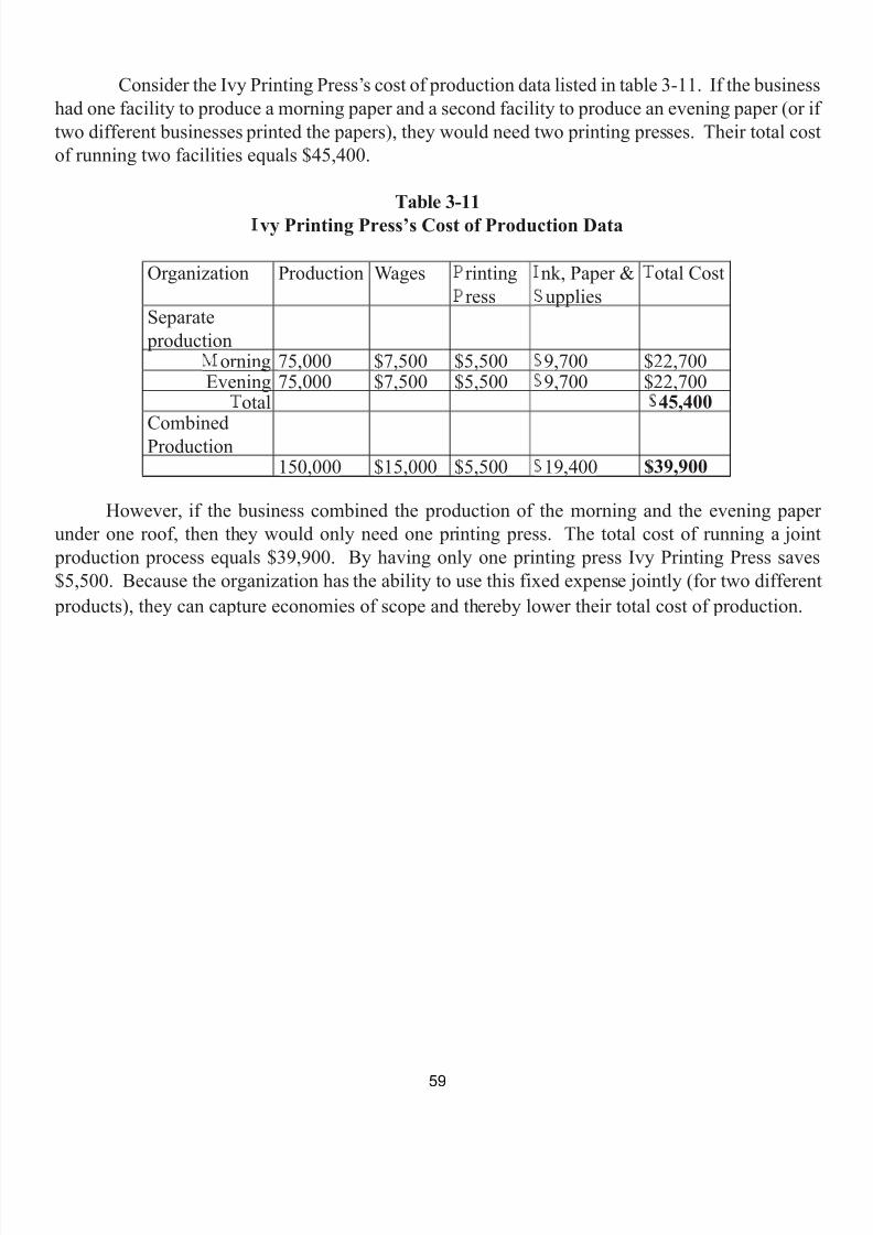
7/21/2019 PSU IVY Fundamentals of Economics
http://slidepdf.com/reader/full/psu-ivy-fundamentals-of-economics 61/118
Consider the Ivy Printing Press’s cost of production data listed in table 3-11. If the businesshad one facility to produce a morning paper and a second facility to produce an evening paper (or iftwo different businesses printed the papers), they would need two printing presses. Their total costof running two facilities equals $45,400.
Table 3-11vy Printing Press’s Cost of Production Data
Organization Production Wages rintingress
nk, Paper &upplies
otal Cost
Separate production
orning 75,000 $7,500 $5,500 9,700 $22,700Evening 75,000 $7,500 $5,500 9,700 $22,700
otal 45,400
CombinedProduction150,000 $15,000 $5,500 19,400 $39,900
However, if the business combined the production of the morning and the evening paperunder one roof, then they would only need one printing press. The total cost of running a joint
production process equals $39,900. By having only one printing press Ivy Printing Press saves$5,500. Because the organization has the ability to use this fixed expense jointly (for two different
products), they can capture economies of scope and thereby lower their total cost of production.
59
7/21/2019 PSU IVY Fundamentals of Economics
http://slidepdf.com/reader/full/psu-ivy-fundamentals-of-economics 62/118
CHAPTER FOUREconomic Per ormance Metrics
1. Introduction
In this chapter, we shift gears from studying the underlying microeconomic foundations of
consumers and businesses to studying the elements of macroeconomic behavior. Macroeconomicsoffers a set of tools and concepts that both economists and policy makers use to try to figure out theoverall pulse of the economy.
The following key concepts are covered in this chapter: nominal gross domestic product,the business cycle, real gross domestic product, transfer payments, the national income identity , thecircular flow, the consumer price index, the producer price index, the inflation rate, the unemploymentrate, discouraged workers, and the types of unemployment.
2. Gross Domestic Product
Figure 4-1 shows “U.S. Real GDP per Capita in 2005 prices over the years 1929-2008.”This title has a lot of information, so let us spend some time explaining each of the components ofthe title. The initials GDP stand for gross domestic product . The term gross tells the reader thatthe data are not adjusted for depreciation. Depreciation is a term that represents the reduction inmarket value of economic capital as it slowly wears out and approaches the end of its useful life.The calculation which adjusts for depreciation is called et domestic product .
Domestic tells us that the data are for output produced and inside the boundaries of theUnited States. Product equals the market value of final goods and services produced over thecourse of a year in the domestic economy. In calculating domestic product, it does not matter thata business is owned by an individual from a foreign nation. If the good or service is producedinside the boundaries of a country it is included in that country’s domestic product calculation. Forexample, a bottle of Coca-Cola produced in Atlanta, GA and sold in the United States is includedin the United States’ domestic product.
On the other hand, income from output sold abroad by a business located abroad, but owned by an American is not included in domestic product. For example, a bottle of Coca-Cola producedand sold in Bratislava, Slovakia is not included in the United States’ domestic product.
______________________ 1 The alternative concept, “national” product, would include products made and income generated by foreign
property owned by U.S. citizens, and would exclude products made and income generated by property in theU.S. that was owned by non-U.S. citizens.
60

7/21/2019 PSU IVY Fundamentals of Economics
http://slidepdf.com/reader/full/psu-ivy-fundamentals-of-economics 63/118
Figure 4-1
U.S Real GDP Per Capita 1929-2008Source: www.bea.gov
Real and 2005 prices inform the reader that the market value of the economic productcalculations are adjusted for changes in the price level – .e , for changes in inflation or deflation.How do you adjust for changes in the price level? The idea is to take the goods and services
produced in 1929, for example, and price them at year 2005 prices. The value of this calculationcaptures what the 1929 bundle would cost in the year 2005. By processing the data in this way forall years, we may then step back and accurately compare the value of goods and services in 1929to those of 2008. This is done in Figure 4-1.
The alternative is to calculate nominal GDP which equals the market value of final goodsand services produced at current year prices. Nominal GDP is almost useless at telling us the truevalue of final goods and services because it confuses changes in the inflation or deflation withchanges in total production. Suppose that quantity produced in the next year stayed unchanged
but prices doubled. Nominal GDP would double. Suppose that the production doubled but pricesstayed the same. Nominal GDP would double. Nominal GDP does not distinguish between thesetwo sources of increases in domestic product. But since it is very important that we do distinguish
between the two sources of increases in domestic product, economists use real GDP and rejectnominal GDP.
61

7/21/2019 PSU IVY Fundamentals of Economics
http://slidepdf.com/reader/full/psu-ivy-fundamentals-of-economics 64/118
Per capita means that total GDP is divided by the U.S. population. This is done to controlfor changes, positive or negative, in the U.S. population.
So that is the breakdown of figure 4-1. eal GDP per capita in 2005 dollars is a measureof the market value of the average domestic labor force production of final goods and servicescontrolling for inflationary and deflationary shifts in the price level.
GDP includes only final goods and services, which are items sold to the end user. A newhome, a coffee frappucino from Starbucks, the cost of your attorney’s time to refinance your currenthome, and a large pepperoni pizza from your favorite pizza joint are all examples of final goods andservices that are included in the government’s calculation of GDP.
Intermediate goods and services are used in the production of final goods and services.Intermediate goods and services are not included in GDP. For example, Starbuck’s purchases coffee
beans – an intermediate good. The coffee bean transaction is not included in GDP. However, whenStarbucks, in the United States, grinds the beans, adds hot water, and sells you a tall coffee the saleis recorded as part of U.S. domestic GDP.
A clear observation from figure 4-1 is that the value of what is produced in the U.S. hasincreased over time. A conservative reading of the figure reveals that the average American is 5.5times better off in 2008 with $43,540 in real GDP relative to 1929 with $7,926 in real GDP.
62
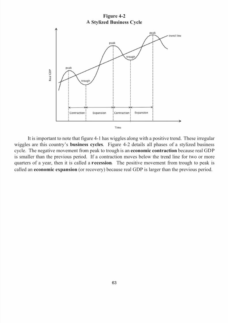
7/21/2019 PSU IVY Fundamentals of Economics
http://slidepdf.com/reader/full/psu-ivy-fundamentals-of-economics 65/118
Figure 4-2 Stylized Business Cycle
It is important to note that figure 4-1 has wiggles along with a positive trend. These irregularwiggles are this country’s business cycles . Figure 4-2 details all phases of a stylized businesscycle. The negative movement from peak to trough is an economic contraction because real GDPis smaller than the previous period. If a contraction moves below the trend line for two or morequarters of a year, then it is called a ecession The positive movement from trough to peak is
called an economic expansion (or recovery) because real GDP is larger than the previous period.
63
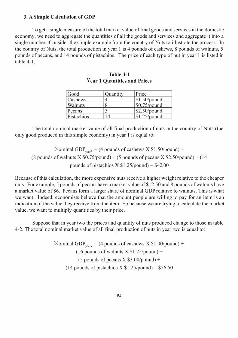
7/21/2019 PSU IVY Fundamentals of Economics
http://slidepdf.com/reader/full/psu-ivy-fundamentals-of-economics 66/118
3. A Simple Calculation of GDP
To get a single measure of the total market value of final goods and services in the domesticeconomy, we need to aggregate the quantities of all the goods and services and aggregate it into asingle number. Consider the simple example from the country of Nuts to illustrate the process. Inthe country of Nuts, the total production in year 1 is 4 pounds of cashews, 8 pounds of walnuts, 5
pounds of pecans, and 14 pounds of pistachios. The price of each type of nut in year 1 is listed intable 4-1.
Table 4-1ear 1 Quantities and Prices
Good Quantity PriceCashews 4 $1.50/poundWalnuts 8 $0.75/poundPecans 5 $2.50/pound
Pistachios 14 $1.25/poundThe total nominal market value of all final production of nuts in the country of Nuts (the
only good produced in this simple economy) in year 1 is equal to:
ominal GDP year = (4 pounds of cashews X $1.50/pound) +(8 pounds of walnuts X $0.75/pound) + (5 pounds of pecans X $2.50/pound) + (14
pounds of pistachios X $1.25/pound) = $42.00
Because of this calculation, the more expensive nuts receive a higher weight relative to the cheapernuts. For example, 5 pounds of pecans have a market value of $12.50 and 8 pounds of walnuts havea market value of $6. Pecans form a larger share of nominal GDP relative to walnuts. This is whatwe want. Indeed, economists believe that the amount people are willing to pay for an item is anindication of the value they receive from the item. So because we are trying to calculate the marketvalue, we want to multiply quantities by their price.
Suppose that in year two the prices and quantity of nuts produced change to those in table4-2. The total nominal market value of all final production of nuts in year two is equal to:
ominal GDP year = (4 pounds of cashews X $1.00/pound) +(16 pounds of walnuts X $1.25/pound) +(5 pounds of pecans X $3.00/pound) +
(14 pounds of pistachios X $1.25/pound) = $56.50
64
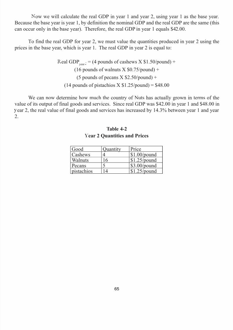
7/21/2019 PSU IVY Fundamentals of Economics
http://slidepdf.com/reader/full/psu-ivy-fundamentals-of-economics 67/118
ow we will calculate the real GDP in year 1 and year 2, using year 1 as the base year.Because the base year is year 1, by definition the nominal GDP and the real GDP are the same (thiscan occur only in the base year). Therefore, the real GDP in year 1 equals $42.00.
To find the real GDP for year 2, we must value the quantities produced in year 2 using the prices in the base year, which is year 1. The real GDP in year 2 is equal to:
eal GDP year = (4 pounds of cashews X $1.50/pound) +(16 pounds of walnuts X $0.75/pound) +(5 pounds of pecans X $2.50/pound) +
(14 pounds of pistachios X $1.25/pound) = $48.00
We can now determine how much the country of Nuts has actually grown in terms of thevalue of its output of final goods and services. Since real GDP was $42.00 in year 1 and $48.00 in
ear 2, the real value of final goods and services has increased by 14.3% between year 1 and year2.
Table 4-2ear 2 Quantities and Prices
Good Quantity PriceCashews 4 $1.00/poundWalnuts 16 $1.25/poundPecans 5 $3.00/pound
pistachios 14 $1.25/pound
65
7/21/2019 PSU IVY Fundamentals of Economics
http://slidepdf.com/reader/full/psu-ivy-fundamentals-of-economics 68/118
4. The Components of GDP
The U.S. Department of Commerce’s Bureau of Economic Analysis (BEA) measures U.S.gross domestic product. The BEA builds the aggregate expenditure measure of gross domestic
product from four main components: consumption expenditures, investment expenditures,government expenditures, and net exports.
• Consumption spending (C) is made up of all the final goods and services that areultimately bought and used by households, except for newly constructed buildings.
• Investment spending (I) is made up of all the final goods and services that become partof the business or residential capital stock, including newly constructed buildings.
• Government spending (G) is made up of all the final goods and services bought by thegovernment, for example, lumber and raw materials purchased and deployed to Iraq forthe reconstruction effort.
o Transfer payments are NOT included in government spending.o xamples of a transfer payment include a social security payment, a welfare
benefit, and unemployment insurance benefit. Each of these involves a payment by the government for which no current goods or services are received by the
overnment.
• Net exports (NX) is made up of the difference between exports (E) and imports (I).o xports are final goods and services produced in the U.S. and purchased by
oreigners living outside the U.S.o mports include all final goods and services produced by foreigners outside the
U.S. and purchased by a member of the domestic population. Combine the domestic consumption (C), investment (I), and government expenditures (G)
plus net exports (NX) and we arrive at the level of aggregate expenditure. Aggregate expenditureis a measure of nominal GDP and it is also known as the ational income identity In summary,
National Income Identity = C + I + G + N = Aggregate Expenditure = Nominal GDP
____________________ See the BEA’s website at www.bea.gov.
66
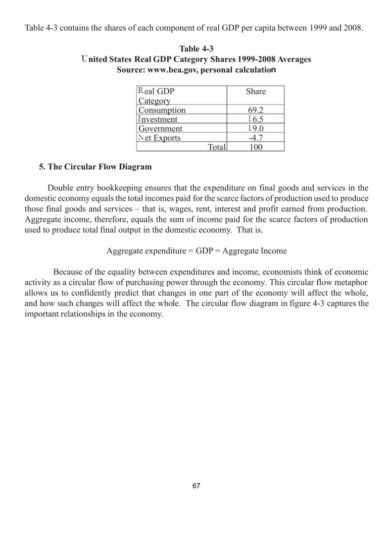
7/21/2019 PSU IVY Fundamentals of Economics
http://slidepdf.com/reader/full/psu-ivy-fundamentals-of-economics 69/118
Table 4-3 contains the shares of each component of real GDP per capita between 1999 and 2008.
Table 4-3nited States Real GDP Category Shares 1999-2008 Averages
Source: www.bea.gov, personal calculatio n
eal GDPCategory
Share
Consumption 69.2nvestment 6.5
Government 9.0et Exports -4.7
Total 100
5. The Circular Flow Diagram
Double entry bookkeeping ensures that the expenditure on final goods and services in thedomestic economy equals the total incomes paid for the scarce factors of production used to producethose final goods and services – that is, wages, rent, interest and profit earned from production.Aggregate income, therefore, equals the sum of income paid for the scarce factors of productionused to produce total final output in the domestic economy. That is,
Aggregate expenditure = GDP = Aggregate Income
Because of the equality between expenditures and income, economists think of economicactivity as a circular flow of purchasing power through the economy. This circular flow metaphorallows us to confidently predict that changes in one part of the economy will affect the whole,and how such changes will affect the whole. The circular flow diagram in figure 4-3 captures theimportant relationships in the economy.
67
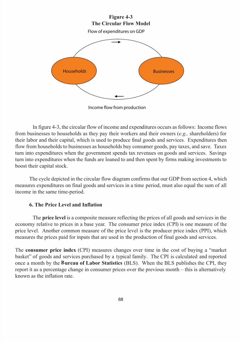
7/21/2019 PSU IVY Fundamentals of Economics
http://slidepdf.com/reader/full/psu-ivy-fundamentals-of-economics 70/118
Figure 4-3The Circular Flow Model
In figure 4-3, the circular flow of income and expenditures occurs as follows: Income flowsfrom businesses to households as they pay their workers and their owners ( e.g., shareholders) fortheir labor and their capital, which is used to produce final goods and services. Expenditures thenflow from households to businesses as households buy consumer goods, pay taxes, and save. Taxesturn into expenditures when the government spends tax revenues on goods and services. Savingsturn into expenditures when the funds are loaned to and then spent by firms making investments to
boost their capital stock.
The cycle depicted in the circular flow diagram confirms that our GDP from section 4, whichmeasures expenditures on final goods and services in a time period, must also equal the sum of allincome in the same time-period.
6. The Price Level and Inflation
The price level is a composite measure reflecting the prices of all goods and services in theeconomy relative to prices in a base year. The consumer price index (CPI) is one measure of the
price level. Another common measure of the price level is the producer price index (PPI), which
measures the prices paid for inputs that are used in the production of final goods and services. The consumer price index (CPI) measures changes over time in the cost of buying a “market
basket” of goods and services purchased by a typical family. The CPI is calculated and reportedonce a month by the ureau of Labor Statistics (BLS). When the BLS publishes the CPI, theyreport it as a percentage change in consumer prices over the previous month – this is alternativelyknown as the inflation rate.
�
68

7/21/2019 PSU IVY Fundamentals of Economics
http://slidepdf.com/reader/full/psu-ivy-fundamentals-of-economics 71/118
To calculate the CPI, the BLS designs the “market basket” so that it closely resembles thegoods and services that consumers are actually buying. Major changes to the market basket aremade by the BLS every five to ten years. Each good or service in the market basket receives aweight equal to its share in the total expenditure by consumers in the base year.
Table 4-4Market Basket Prices
Year Price of Starbuck’scoffee/12 oz. (tall)
rice of basic cable/onth
rice of Milk/gallon
2020 (base year) $1.40 $35.00 $2.002021 $1.45 $40.00 $2.502022 $1.50 $45.00 $3.252023 $1.50 $50.00 $4.25
Consider the market basket in table 4-4 which we will use to calculate the CPI. In the baseear, assume our consumers spend a total of $1,035: suppose consumers buy $511.00 (49.4%) worthof Starbuck’s coffee, $420.00 (40.6%) worth of basic cable, and $104.00 (10%) worth of milk. Theconsumer price index is calculated as follows, where a goods’ weight equals its percentage of theconsumer’s total expenditure.
CPI = X(Starbuck’s coffee weight ) +
X asic cable weight ) +
X ilk weight ) .
CPI = (49.4) +
(40.6) +
X(10.0)
rice of Starbuck’s coffee todayrice of Starbuck’s coffee in base year
rice of basic cable todayrice of basic cable in base year
rice of milk todayrice of milk in base year
rice o Starbuck’s co ee toda .
rice of basic cable today
$35.00
rice of milk today$2.00
69

7/21/2019 PSU IVY Fundamentals of Economics
http://slidepdf.com/reader/full/psu-ivy-fundamentals-of-economics 72/118
In the base year, the CPI, by definition, equals 100. This is clearly demonstrated when 2020 pricesare inserted for today’s prices:
CPI 020 (49.4)+ (40.6)+ (10.0) = 100
In reality, the market basket does not change for as long as a ten year period of time. Theweights assigned to each good only change when the market-basket changes. Therefore, we willassume that our market basket and weights do not change over the 2020-2023 time period.
The CPI for the years 2021-2023 are:
CPI 021 = (49.4)+ (40.6)+ (10.0) = 110.1
CPI 022 = X (49.4)+ X (40.6)+ X (10.0) = 121.4
CPI 023 (49.4)+ (40.6)+ (10.0) = 132.2
Changes in the cost of the market basket from one year to the next are commonly referredto as changes in the cost of living or as the nflation rate The inflation rate in 2021 is:
Inflation Rate 2021 = X 100 = X 100 = 10.1%
The inflation rates for 2022 and 2023 are:
Inflation Rate 2022 = X 100 = X 100 = 10.26%
Inflation Rate 2023 = 100 = 00 = 8.90%
$1.40.
35.00 .
2.00 .
$1.45$1.40
$40.00 .
$2.50 .
$1.50$1.40
45.00 .
3.25 .
$1.50$1.40 50.00 . 4.25 .
CPI 2021 - CPI 020 PI 020
(110.1 - 100)100
CPI 022 - CPI 021 PI 021
121.4 - 110.1 .
CPI 2023 - CPI 022 PI 022
132.2 - 121.4 .
70
7/21/2019 PSU IVY Fundamentals of Economics
http://slidepdf.com/reader/full/psu-ivy-fundamentals-of-economics 73/118
The federal government reports the CPI every month based on price data collected fromabout 23,000 retail and service establishments in 87 urban areas throughout the country. Thetwelve monthly changes in consumer prices over the course of the year are added up and becomethat year’s inflation rate. When we speak of the inflation rate, we speak of it as a percent per year To speak of the inflation rate without a unit of time attached is incomplete. But people do, and wealways assume that, when the period of time is omitted, the inflation rate is being given in percent
per year.
The roducer price index (PPI) measures the average change over time in the pricesreceived by domestic producers. The PPI is also calculated by the BLS. The PPI sample includesover 25,000 establishments providing approximately 100,000 price quotations per month. Goodsand services included in the PPI are weighted by value-of-shipments data contained in the 1997economic census. The PPI is calculated in exactly the same way we calculated the CPI, but ituses producer prices and a fixed production market basket instead of consumer prices and a fixedconsumer market basket. Changes in the cost of the PPI over a period of time offer another measureof the inflation rate. The rate of change in the cost of the PPI is calculated as follows:
Inflation Rate current perio 100
_________________ See www.bls.gov for more details.
PPI urrent period - PPI previous period
PPI revious perio
71
7/21/2019 PSU IVY Fundamentals of Economics
http://slidepdf.com/reader/full/psu-ivy-fundamentals-of-economics 74/118
6. Unemployment
The nemployment rate is a key indicator of economic performance and it is one of themost widely reported government statistics. Indeed, keeping unemployment low is a frequentlyquoted goal of macroeconomic policy makers – most notably the President of the United States.
The Bureau of Labor Statistic (BLS) calculates the unemployment rate by conducting60,000 personal and telephone interviews of households in a nationwide survey called the CurrentPopulation Survey (CPS). The CPS provides a comprehensive body of data on the labor force,employment, unemployment, and persons not in the labor force. The BLS classifies the people thatit interviews into four categories:
I. Those who are employed – individuals with some kind of job.II. Those who are out of the labor force – individuals who do not want a job right
now.III. Those who do want a job right now, but who have no been looking for work
because they do not think they could find one they would take.IV. Those who do want a job right now, have been looking for work , but have not
ound a job that they would take.
The abor force is defined as group “I” plus group “IV”, those who have a job plus thoselooking for jobs:
Labor Force = (Employed) + (Have Been Looking for Work)
The unemployment rate is defined to equal group “IV” divided by the labor force:
For example, if the number of people employed equaled 8 million and the number of peoplelooking for work equaled 2 million, then the labor force equals 10 million. The unemployment ratein this example would equal twenty percent (2 million people/10 million people).
Unemployment Rate = Have Been Looking for Work
Labor Force Have Been Looking for Work
(Employed) + (Have Been Looking for Work)=
72
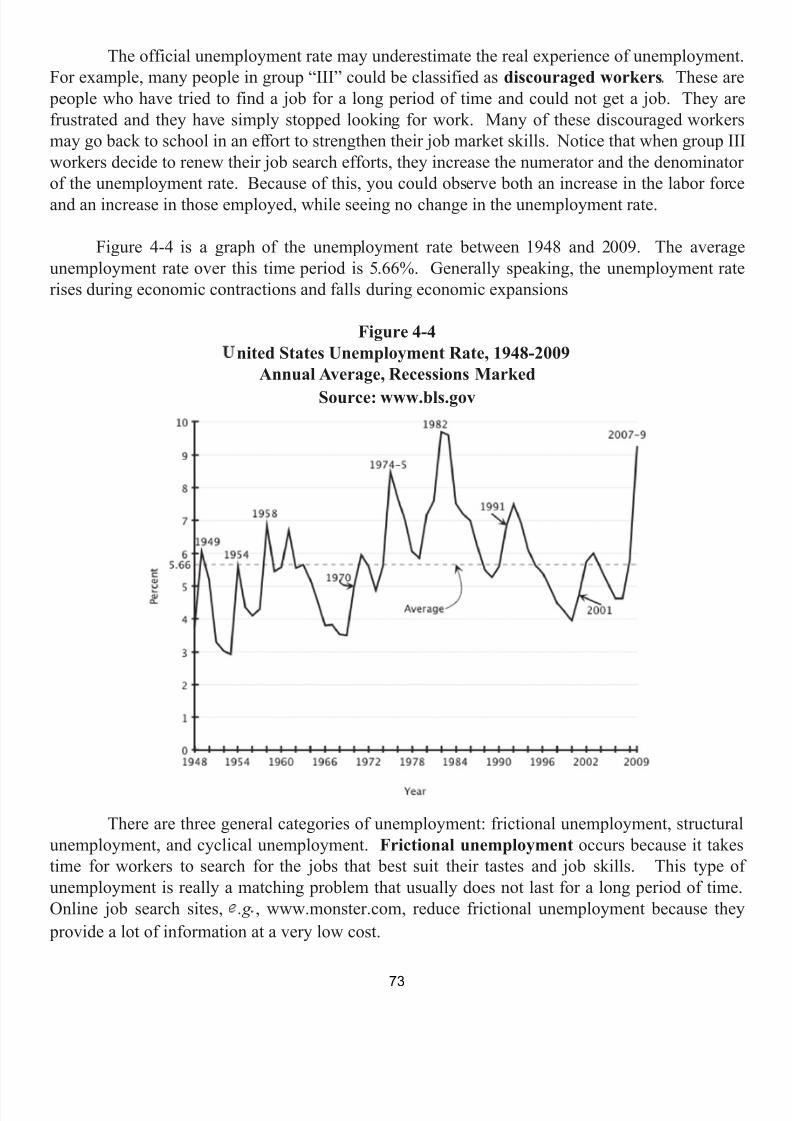
7/21/2019 PSU IVY Fundamentals of Economics
http://slidepdf.com/reader/full/psu-ivy-fundamentals-of-economics 75/118
The official unemployment rate may underestimate the real experience of unemployment.For example, many people in group “III” could be classified as discouraged workers These are
people who have tried to find a job for a long period of time and could not get a job. They arefrustrated and they have simply stopped looking for work. Many of these discouraged workersmay go back to school in an effort to strengthen their job market skills. Notice that when group IIIworkers decide to renew their job search efforts, they increase the numerator and the denominatorof the unemployment rate. Because of this, you could observe both an increase in the labor forceand an increase in those employed, while seeing no change in the unemployment rate.
Figure 4-4 is a graph of the unemployment rate between 1948 and 2009. The averageunemployment rate over this time period is 5.66%. Generally speaking, the unemployment raterises during economic contractions and falls during economic expansions
Figure 4-4nited States Unemployment Rate, 1948-2009
Annual Average, Recessions MarkedSource: www.bls.gov
There are three general categories of unemployment: frictional unemployment, structuralunemployment, and cyclical unemployment. Frictional unemployment occurs because it takestime for workers to search for the jobs that best suit their tastes and job skills. This type ofunemployment is really a matching problem that usually does not last for a long period of time.Online job search sites, .g , www.monster.com, reduce frictional unemployment because they
provide a lot of information at a very low cost.
73
7/21/2019 PSU IVY Fundamentals of Economics
http://slidepdf.com/reader/full/psu-ivy-fundamentals-of-economics 76/118
Structural unemployment occurs because the number of jobs available in a labor marketis insufficient to provide jobs for all that want a job. For example, many manufacturing jobs are
being eliminated because computers have replaced work once performed by humans. Thus, despiteincreased output in these markets, there are fewer jobs available. Cyclical unemployment isunemployment that occurs because of declines in the economy’s aggregate output (GDP) duringeconomic contractions and recessions.
74
7/21/2019 PSU IVY Fundamentals of Economics
http://slidepdf.com/reader/full/psu-ivy-fundamentals-of-economics 77/118
CHAPTER FIVEMoney & Ban ing
1. Introduction
What is money? Money is any asset that may be used to carry out a transaction between a buyer and a seller. The most familiar asset is currency, dollar bills and coins, but other examplesof money include bank accounts and money market accounts. This chapter examines the role ofmoney in the economy.
Key concepts covered in this chapter include: the functions of money, the types of money,classifications of the money supply, the money creation process, bank reserves, required and desiredreserve deposit ratio, the Federal Reserve, monetary policy, the price level, the value of money, and
money supply and demand.
2. The Functions and Types of Money
The three basic functions of money are a medium of exchange, a store of value, and a unit-of-account. Money is a edium of exchange because money makes exchange easier. In a bartereconomy , an economy with no money, people spend a lot of time carrying out exchanges. In suchan economy, there must be a double coincidence of wants for exchange to take place. For example,someone who had a piece of cheese and wanted a glass of wine would have to hunt around for a
bar that was willing to trade a glass of wine for a piece of cheese. But in a monetary economy, pieces of paper may be used to buy a glass of wine. The bar owner will accept these pieces of paper because, in turn, he/she believes that others will accept them, and so on. Money, therefore, solvesthe transaction cost problem of a barter economy.
Money is also a store of value . People will hold money only if they believe it will continueto have some value, so money can operate as a medium of exchange only if it serves as a store ofvalue. For example, using fish as money is a poor choice because its purchasing power literallydeteriorates. Rabbits are also a poor choice because the rapid increase in supply would decrease the
purchasing power of any one rabbit. Any such choice will quickly be replaced by a more durableasset that is a better store of value. The industry standard, of course, is paper money because it isgenerally a good store of value.
75

7/21/2019 PSU IVY Fundamentals of Economics
http://slidepdf.com/reader/full/psu-ivy-fundamentals-of-economics 78/118
Lastly, money is a nit-of-account Money is a convenient and widely recognized measurefor accounting and transactions; it is a yardstick for measuring the value of all goods and services.In the United States, for example, people negotiate contracts in dollars and post prices in dollars
because it is convenient and because they know that others will understand.
Paper money that has no intrinsic value, .g. , the U.S. dollar, is known as fiat money Fiatmoney is paper money that derives its status as money from the power of the state, or by fiat. It ismoney because the government says that it is money, it otherwise has no real value. Fiat money can
be contrasted with commodity money , which exists when some intrinsically valuable good alsoserves as money. Gold is an example of commodity money because it has value even if it were notused as money.
3. Measuring the Money Supply
When people talk of the quantity of money or the money supply , they are usually thinkingabout currency – bills and coins. Yet, currency is not the only asset that you can use to purchasegoods and services. The Federal Reserve System, the central bank of the United States, classifiesseveral alternative definitions of money. One of the Federal Reserve’s definitions of money supplyis called M1, while another is called M2.
The most narrowly defined money supply is M1, which includes currency, traveler’s checks,demand deposits, and other checkable deposits. M2 is more expansive. It includes everything inM1, plus savings deposits, small time deposits, money market mutual funds, and a few other minorcategories. Table 5-1 defines the measures of money. Figure 5-1 shows the annual average of M1and M2 from 1959 to 2009. Ultimately, which definition of money one chooses is largely a matter
of personal preference. The most common definition of money is M1.
__________________ There are two other definitions of money, M3 and M4, which we will not cover in this book.
76
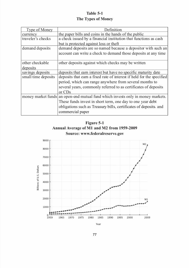
7/21/2019 PSU IVY Fundamentals of Economics
http://slidepdf.com/reader/full/psu-ivy-fundamentals-of-economics 79/118
Table 5-1The Types of Money
ype of Money Definitioncurrency the paper bills and coins in the hands of the public traveler’s checks a check issued by a financial institution that functions as cash
but is protected against loss or theft demand deposits demand deposits are so named because a depositor with such an
account can write a check to demand those deposits at any time
other checkabledeposits
other deposits against which checks may be written
savings deposits deposits that earn interest but have no specific maturity date small time deposits deposits that earn a fixed rate of interest if held for the specified
period, which can range anywhere from several months toseveral years, commonly referred to as certificates of deposits
or CDsmoney market funds an open-end mutual fund which invests only in money markets.These funds invest in short term, one day to one year debtobligations such as Treasury bills , certificates of deposits andcommercial paper
Figure 5-1Annual Average of M1 and M2 from 1959-2009
Source: www.federalreserve.gov
77
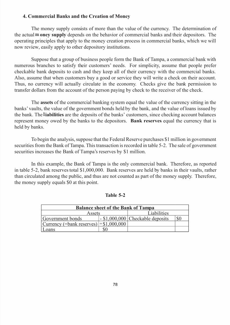
7/21/2019 PSU IVY Fundamentals of Economics
http://slidepdf.com/reader/full/psu-ivy-fundamentals-of-economics 80/118
4. Commercial Banks and the Creation of Money
The money supply consists of more than the value of the currency. The determination ofthe actual oney supply depends on the behavior of commercial banks and their depositors. Theoperating principles that apply to the money creation process in commercial banks, which we willnow review, easily apply to other depository institutions.
Suppose that a group of business people form the Bank of Tampa, a commercial bank withnumerous branches to satisfy their customers’ needs. For simplicity, assume that people prefercheckable bank deposits to cash and they keep all of their currency with the commercial banks.Also, assume that when customers buy a good or service they will write a check on their account.Thus, no currency will actually circulate in the economy. Checks give the bank permission totransfer dollars from the account of the person paying by check to the receiver of the check.
The assets of the commercial banking system equal the value of the currency sitting in the banks’ vaults, the value of the government bonds held by the bank, and the value of loans issued bythe bank. The iabilities are the deposits of the banks’ customers, since checking account balancesrepresent money owed by the banks to the depositors. Bank reserves equal the currency that isheld by banks.
To begin the analysis, suppose that the Federal Reserve purchases $1 million in governmentsecurities from the Bank of Tampa. This transaction is recorded in table 5-2. The sale of governmentsecurities increases the Bank of Tampa’s reserves by $1 million.
In this example, the Bank of Tampa is the only commercial bank. Therefore, as reported
in table 5-2, bank reserves total $1,000,000. Bank reserves are held by banks in their vaults, ratherthan circulated among the public, and thus are not counted as part of the money supply. Therefore,the money supply equals $0 at this point.
Table 5-2
Balance sheet of the Bank of Tampa Assets Liabilities
Government bonds - $1,000,000 Checkable deposits $0Currency (=bank reserves) $1,000,000Loans $0
78
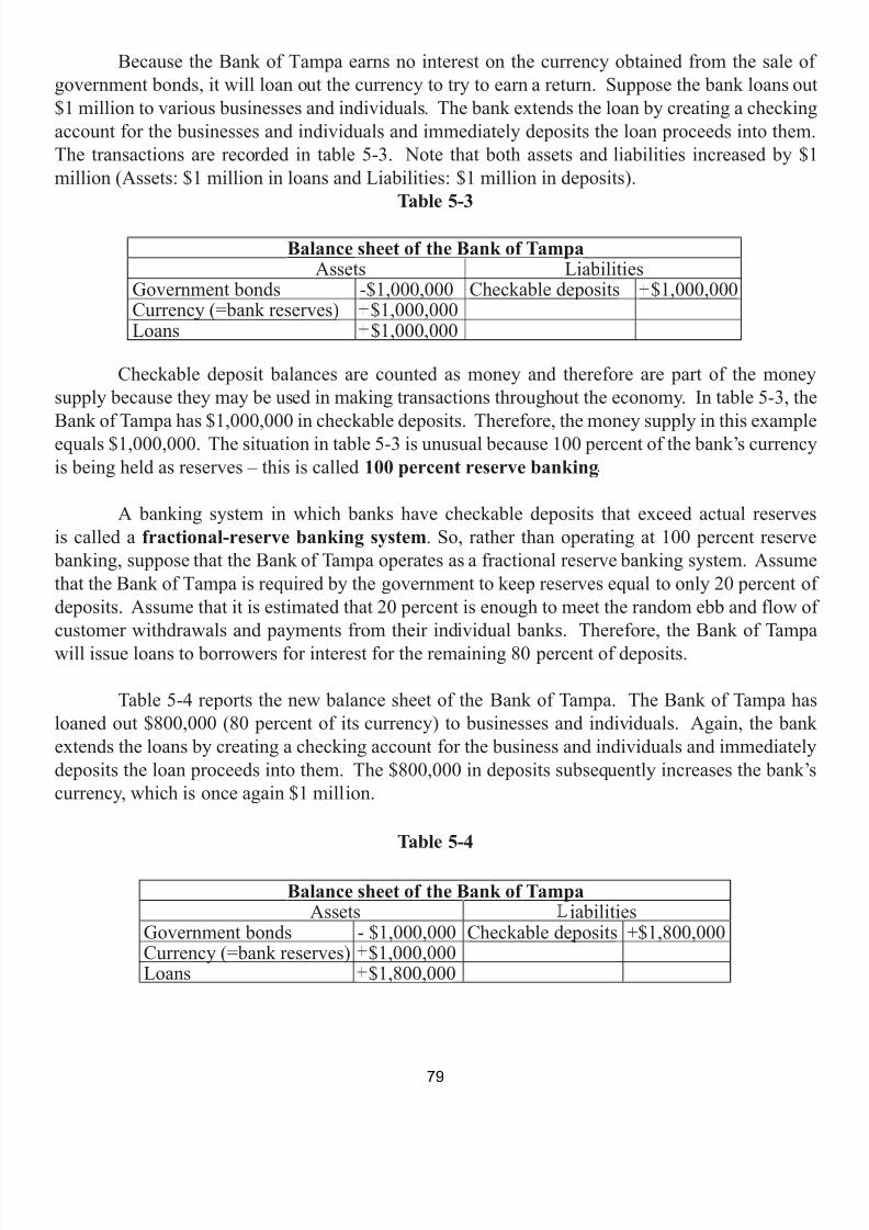
7/21/2019 PSU IVY Fundamentals of Economics
http://slidepdf.com/reader/full/psu-ivy-fundamentals-of-economics 81/118
Because the Bank of Tampa earns no interest on the currency obtained from the sale ofgovernment bonds, it will loan out the currency to try to earn a return. Suppose the bank loans out$1 million to various businesses and individuals. The bank extends the loan by creating a checkingaccount for the businesses and individuals and immediately deposits the loan proceeds into them.The transactions are recorded in table 5-3. Note that both assets and liabilities increased by $1million (Assets: $1 million in loans and Liabilities: $1 million in deposits).
Table 5-3
Balance sheet of the Bank of Tampa Assets Liabilities
Government bonds -$1,000,000 Checkable deposits $1,000,000Currency (=bank reserves) $1,000,000Loans $1,000,000
Checkable deposit balances are counted as money and therefore are part of the moneysupply because they may be used in making transactions throughout the economy. In table 5-3, theBank of Tampa has $1,000,000 in checkable deposits. Therefore, the money supply in this exampleequals $1,000,000. The situation in table 5-3 is unusual because 100 percent of the bank’s currencyis being held as reserves – this is called 100 percent reserve banking
A banking system in which banks have checkable deposits that exceed actual reservesis called a fractional-reserve banking system . So, rather than operating at 100 percent reserve
banking, suppose that the Bank of Tampa operates as a fractional reserve banking system. Assumethat the Bank of Tampa is required by the government to keep reserves equal to only 20 percent ofdeposits. Assume that it is estimated that 20 percent is enough to meet the random ebb and flow ofcustomer withdrawals and payments from their individual banks. Therefore, the Bank of Tampawill issue loans to borrowers for interest for the remaining 80 percent of deposits.
Table 5-4 reports the new balance sheet of the Bank of Tampa. The Bank of Tampa hasloaned out $800,000 (80 percent of its currency) to businesses and individuals. Again, the bankextends the loans by creating a checking account for the business and individuals and immediatelydeposits the loan proceeds into them. The $800,000 in deposits subsequently increases the bank’scurrency, which is once again $1 million.
Table 5-4
Balance sheet of the Bank of Tampa Assets iabilities
Government bonds - $1,000,000 Checkable deposits +$1,800,000Currency (=bank reserves) $1,000,000Loans $1,800,000
79
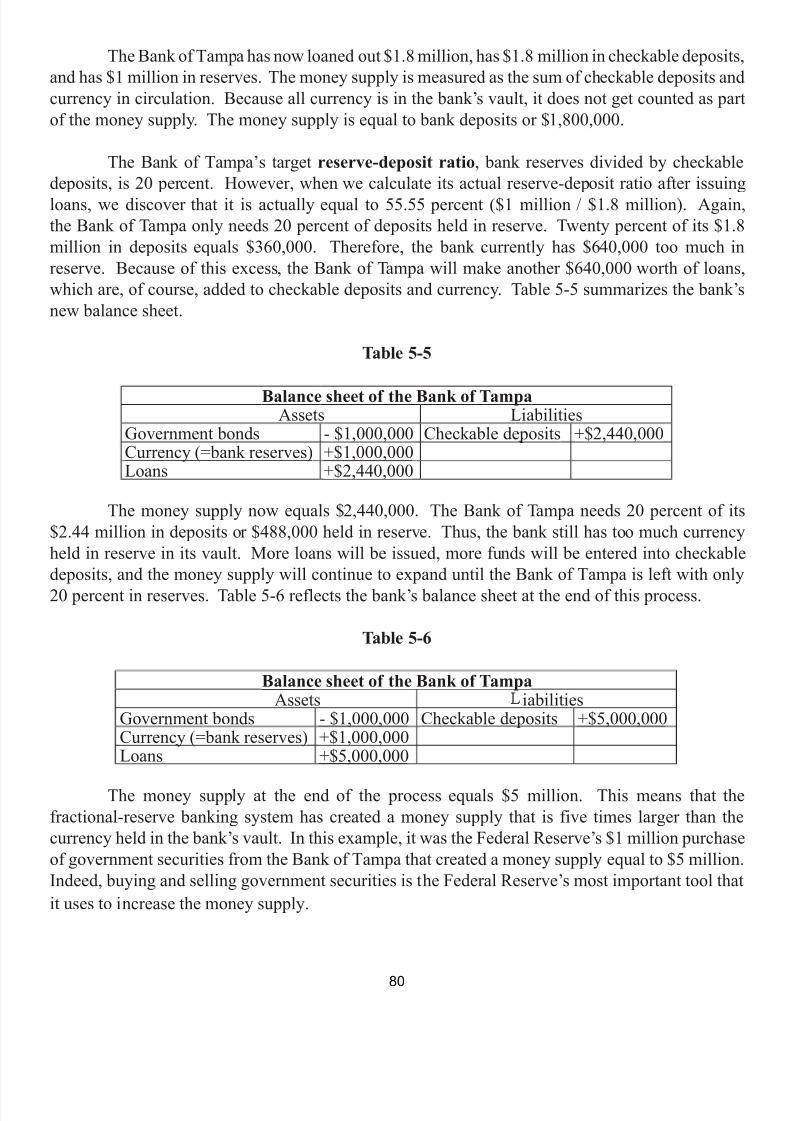
7/21/2019 PSU IVY Fundamentals of Economics
http://slidepdf.com/reader/full/psu-ivy-fundamentals-of-economics 82/118
The Bank of Tampa has now loaned out $1.8 million, has $1.8 million in checkable deposits,and has $1 million in reserves. The money supply is measured as the sum of checkable deposits andcurrency in circulation. Because all currency is in the bank’s vault, it does not get counted as partof the money supply. The money supply is equal to bank deposits or $1,800,000.
The Bank of Tampa’s target reserve-deposit ratio , bank reserves divided by checkabledeposits, is 20 percent. However, when we calculate its actual reserve-deposit ratio after issuingloans, we discover that it is actually equal to 55.55 percent ($1 million / $1.8 million). Again,the Bank of Tampa only needs 20 percent of deposits held in reserve. Twenty percent of its $1.8million in deposits equals $360,000. Therefore, the bank currently has $640,000 too much inreserve. Because of this excess, the Bank of Tampa will make another $640,000 worth of loans,which are, of course, added to checkable deposits and currency. Table 5-5 summarizes the bank’snew balance sheet.
Table 5-5
Balance sheet of the Bank of Tampa Assets Liabilities
Government bonds - $1,000,000 Checkable deposits +$2,440,000Currency (=bank reserves) +$1,000,000Loans +$2,440,000
The money supply now equals $2,440,000. The Bank of Tampa needs 20 percent of its$2.44 million in deposits or $488,000 held in reserve. Thus, the bank still has too much currencyheld in reserve in its vault. More loans will be issued, more funds will be entered into checkabledeposits, and the money supply will continue to expand until the Bank of Tampa is left with only20 percent in reserves. Table 5-6 reflects the bank’s balance sheet at the end of this process.
Table 5-6
Balance sheet of the Bank of Tampa Assets iabilities
Government bonds - $1,000,000 Checkable deposits +$5,000,000Currency (=bank reserves) +$1,000,000Loans +$5,000,000
The money supply at the end of the process equals $5 million. This means that thefractional-reserve banking system has created a money supply that is five times larger than thecurrency held in the bank’s vault. In this example, it was the Federal Reserve’s $1 million purchaseof government securities from the Bank of Tampa that created a money supply equal to $5 million.Indeed, buying and selling government securities is the Federal Reserve’s most important tool thatit uses to increase the money supply.
80
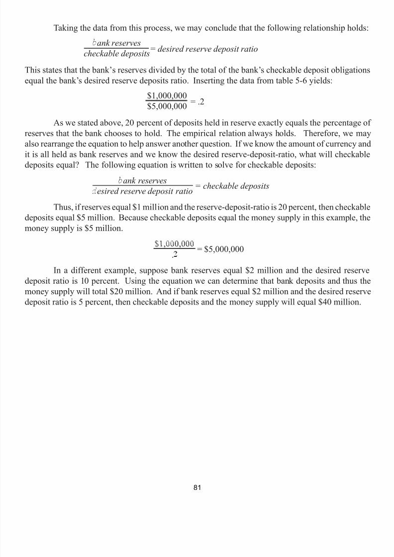
7/21/2019 PSU IVY Fundamentals of Economics
http://slidepdf.com/reader/full/psu-ivy-fundamentals-of-economics 83/118
Taking the data from this process, we may conclude that the following relationship holds:
= desired reserve deposit ratio
This states that the bank’s reserves divided by the total of the bank’s checkable deposit obligationsequal the bank’s desired reserve deposits ratio. Inserting the data from table 5-6 yields:
= .2
As we stated above, 20 percent of deposits held in reserve exactly equals the percentage ofreserves that the bank chooses to hold. The empirical relation always holds. Therefore, we mayalso rearrange the equation to help answer another question. If we know the amount of currency andit is all held as bank reserves and we know the desired reserve-deposit-ratio, what will checkabledeposits equal? The following equation is written to solve for checkable deposits:
= checkable deposits
Thus, if reserves equal $1 million and the reserve-deposit-ratio is 20 percent, then checkabledeposits equal $5 million. Because checkable deposits equal the money supply in this example, themoney supply is $5 million.
= $5,000,000
In a different example, suppose bank reserves equal $2 million and the desired reservedeposit ratio is 10 percent. Using the equation we can determine that bank deposits and thus the
money supply will total $20 million. And if bank reserves equal $2 million and the desired reservedeposit ratio is 5 percent, then checkable deposits and the money supply will equal $40 million.
ank reservescheckable deposits
$1,000,000$5,000,000
ank reserves
esired reserve deposit ratio
.
81
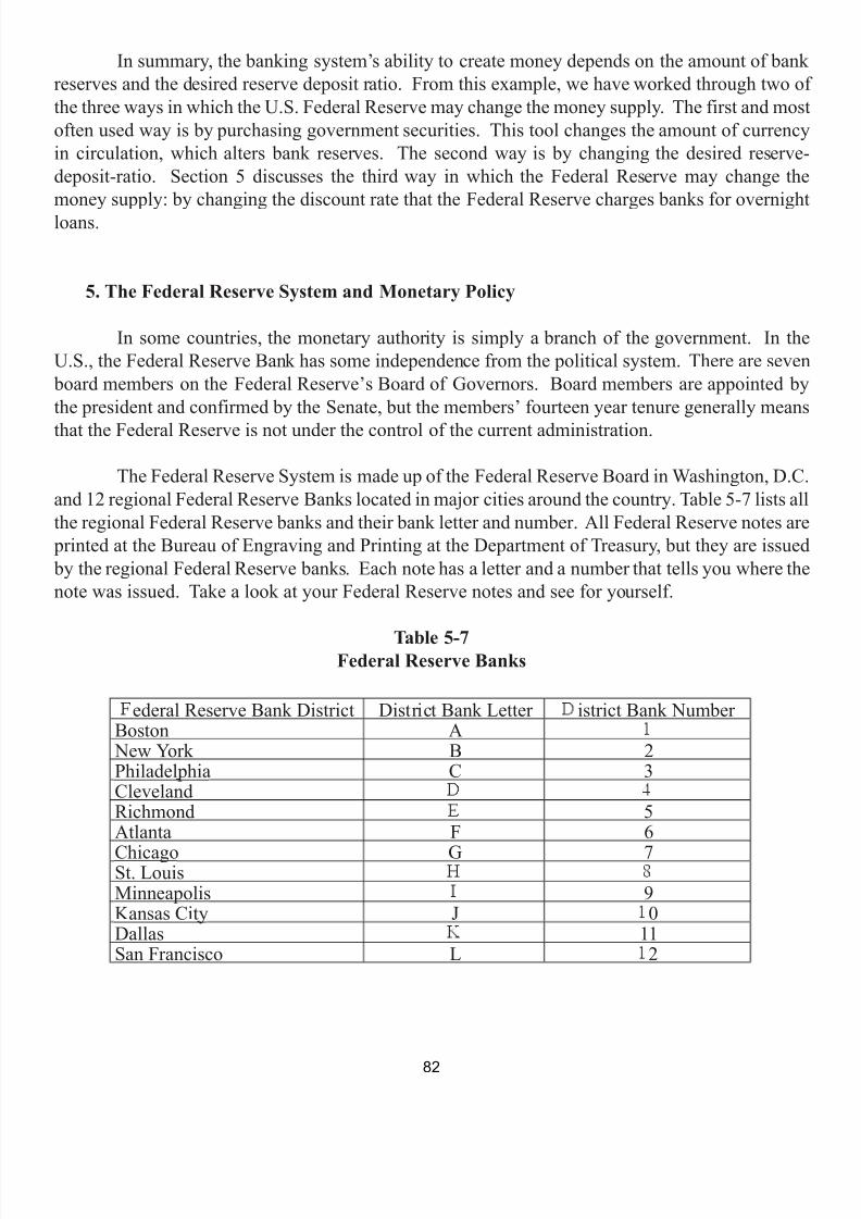
7/21/2019 PSU IVY Fundamentals of Economics
http://slidepdf.com/reader/full/psu-ivy-fundamentals-of-economics 84/118
In summary, the banking system’s ability to create money depends on the amount of bankreserves and the desired reserve deposit ratio. From this example, we have worked through two ofthe three ways in which the U.S. Federal Reserve may change the money supply. The first and mostoften used way is by purchasing government securities. This tool changes the amount of currencyin circulation, which alters bank reserves. The second way is by changing the desired reserve-deposit-ratio. Section 5 discusses the third way in which the Federal Reserve may change themoney supply: by changing the discount rate that the Federal Reserve charges banks for overnightloans.
5. The Federal Reserve System and Monetary Policy
In some countries, the monetary authority is simply a branch of the government. In theU.S., the Federal Reserve Bank has some independence from the political system. There are seven
board members on the Federal Reserve’s Board of Governors. Board members are appointed bythe president and confirmed by the Senate, but the members’ fourteen year tenure generally meansthat the Federal Reserve is not under the control of the current administration.
The Federal Reserve System is made up of the Federal Reserve Board in Washington, D.C.and 12 regional Federal Reserve Banks located in major cities around the country. Table 5-7 lists allthe regional Federal Reserve banks and their bank letter and number. All Federal Reserve notes are
printed at the Bureau of Engraving and Printing at the Department of Treasury, but they are issued by the regional Federal Reserve banks. Each note has a letter and a number that tells you where thenote was issued. Take a look at your Federal Reserve notes and see for yourself.
Table 5-7Federal Reserve Banks
ederal Reserve Bank District District Bank Letter istrict Bank Number Boston A
New York B 2Philadelphia C 3ClevelandRichmond 5Atlanta F 6
Chicago G 7St. LouisMinneapolis 9Kansas City J 0Dallas 11San Francisco L 2
82
7/21/2019 PSU IVY Fundamentals of Economics
http://slidepdf.com/reader/full/psu-ivy-fundamentals-of-economics 85/118
The control of the money supply by the Federal Reserve Bank is known as onetarypolicy The Federal Reserve has three tools at its disposal to alter the money supply: open marketoperations, reserve requirement changes, and changes to the Federal Reserve’s discount rate .
The Banking Acts of 1933 and 1935 centralized power of the Federal Reserve in WashingtonD.C., and established the ederal Open Market Committee (FOMC). The FOMC is made upof 7 members of the Board of Governors and 5 of the 12 regional bank presidents. All 12 regional
bank presidents are present at FOMC meetings, but only 5 vote at any given meeting. Voting rightsrotate among the regional bank presidents, except the New York Federal bank president alwaysvotes.
The FOMC meets about every six weeks in Washington, D.C., in order to discuss thecondition of the economy and consider changes to monetary policy, most important of which is openmarket operations. Open market operations are purchases and sales of government securities bythe Federal Reserve in an effort to influence the money supply. When the Federal Reserve decidesto purchase government securities (e.g., Treasury bills), it is choosing to increase the money supplyand when it decides to sell government securities it is choosing to reduce the money supply.
The second monetary policy option is to change the required reserve deposit ratio. Asdiscussed in section 4, an increase in the required reserve deposit ratio will lead to a decrease inthe money supply and a decrease in the required reserve deposit ratio will lead to an increase in themoney supply.
The third monetary policy tool is the Federal Reserve discount rate, which is the interestrate on loans that the Federal Reserve charges to other banks. A bank borrows from the Federal
Reserve when it has too few reserves to meet reserve requirements. This might occur because the bank made too many loans or because it has experienced too many recent withdrawals. When theFederal Reserve increases the discount rate, it discourages banks from borrowing reserves fromthe Federal Reserve. Thus, an increase in the discount rate reduces the quantity of reserves inthe banking system, which in turn reduces the money supply. And a decrease in the discountrate, encourages borrowing reserves from the Federal Reserve, which in turn increases the moneysupply.
83
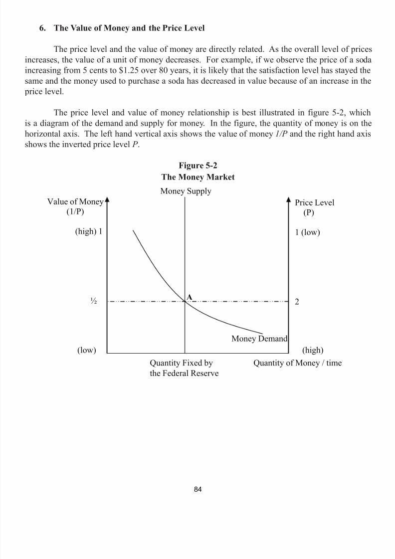
7/21/2019 PSU IVY Fundamentals of Economics
http://slidepdf.com/reader/full/psu-ivy-fundamentals-of-economics 86/118
6. The Value of Money and the Price Level
The price level and the value of money are directly related. As the overall level of pricesincreases, the value of a unit of money decreases. For example, if we observe the price of a sodaincreasing from 5 cents to $1.25 over 80 years, it is likely that the satisfaction level has stayed thesame and the money used to purchase a soda has decreased in value because of an increase in the
price level.
The price level and value of money relationship is best illustrated in figure 5-2, whichis a diagram of the demand and supply for money. In the figure, the quantity of money is on thehorizontal axis. The left hand vertical axis shows the value of money 1/P and the right hand axisshows the inverted price level P .
Figure 5-2The Money Market
Value of Money
(1/P)
(high) 1
½
Price Level(P)
1 (low)
2
Quantity Fixed bythe Federal Reserve
Quantity of Money / time
A
(low) (high)
Money Supply
Money Demand
84

7/21/2019 PSU IVY Fundamentals of Economics
http://slidepdf.com/reader/full/psu-ivy-fundamentals-of-economics 87/118
The supply of money is determined by the Federal Reserve and the overall banking system,as discussed in sections 3 and 4 above. Three general policies shift the supply of money curve.
• Firstly, if the Federal Reserve buys government bonds in open market operations, it pays
out dollars and causes the money supply to shift to the right. When it sells government bonds in open market operations, it takes in dollars and causes the supply of money curveto shift to the left.
• Secondly, if the Federal Reserve decreases the required reserve requirement, the supplyof money will shift to the right. And if the Federal Reserve increases the required reservedeposit ratio, the supply of money will shift to the left.
• Lastly, if the Federal Reserve decreases the discount rate, the supply of money will shift tothe right. When they increase the discount rate, the supply of money will shift to the left.
The demand for money reflects how much wealth people want to hold in liquid form atany point in time. The most important determinant of how much money people demand is the
price level. Because money is a medium of exchange, they demand it to buy goods and servicesthroughout their ordinary business of life. Other assets like real estate, stocks, or bonds are notvery liquid and cannot be easily used to buy goods and services. Thus, the higher the price level,the larger will be the quantity demanded of money (e.g., cash and checking account funds), so that
people can fulfill their transactions for goods and services.
In the long run, the overall level of price adjusts to the level at which the demand for moneyequals the supply of money. This is shown in figure 5-2.
• At equilibrium the price level or the price of goods measured in money is 2. This number
tells you that one basket of goods and services will cost you $2.• On the other hand, the value of money measured in terms of goods and services is ½. And
this number tells you that you are able to buy one-half of a basket of goods and serviceswith $1.
If for some reason the price level was equal to 3, people would demand a quantity of moneythat exceeded the quantity supplied by the Federal Reserve. As a result, the price level woulddecrease (and the value of money would increase) until equilibrium was again reached. When the
price level is lower than the equilibrium price level, the market will adjust back to equilibrium in
the long run.
___________________ We only consider the direct effect of the following policy changes. There are indirect effects that are
ignored here.
85
7/21/2019 PSU IVY Fundamentals of Economics
http://slidepdf.com/reader/full/psu-ivy-fundamentals-of-economics 88/118
Monetary policy shifts the supply of money. If the Federal Reserve increases the supplyof money, the price level in the economy increases and the value of money decreases. Recall fromchapter 4, that an increase in the price level from one period to the next is called inflation . In thiscase, because the Federal Reserve has increased the supply of money, it caused inflation in theeconomy.
Alternatively, if the Federal Reserve decreases the supply of money, the price level in theeconomy decreases and the value of money increases. A decrease in the price level from one periodto the next is called deflation .
86

7/21/2019 PSU IVY Fundamentals of Economics
http://slidepdf.com/reader/full/psu-ivy-fundamentals-of-economics 89/118
CHAPTER SIX Aggregate Deman & Aggregate Supp y
1. Introduction
In chapters four and five we looked at the determinants of macroeconomic variables in thelong run. In macroeconomics, there are two major differences between the short run and the longrun. Firstly, in the long run we assume that there is a separation of real (adjusted for price levelchanges) and nominal (not adjusted for price level changes) variables. This separation of real andnominal variables is a concept that is formally called the classical dichotomy . Secondly, in the longrun, the money supply affects only nominal variables and not real variables. This is demonstrated inchapter five’s figure 5-2, where a change in the money supply by the Federal Reserve strictly causesthe price level to change, .e. it causes inflation or deflation, and it has no effect on the real value
people place on goods and services. This second idea is formally called onetary neutrality .
However, when we look at year-to-year changes in the economy, the assumption of monetaryneutrality is no longer appropriate. In this chapter, we will drop the assumption of monetaryneutrality and develop a model of aggregate demand and aggregate supply that deals with short runeconomic fluctuations.
In this model, the first variable is real gross domestic product (real GDP) and the secondvariable is the overall rice level (P) which is measured by the consumer price index or someother index of prices in the economy. Notice, that this short run model reflects a breakdown ofthe classical dichotomy because it uses a nominal variable, the price level, and a real variable, realGDP, at the same time.
Key concepts introduced in this chapter include: classical dichotomy, monetary neutrality,aggregate demand, the interest rate effect, the wealth effect, the open economy effect, the realexchange rate, the short run aggregate supply, the profit effect, the misperceptions effect, the menucosts effect, long run aggregate supply, potential real GDP, the natural rate of unemployment,inflationary gap, deflationary gap, fiscal policy, automatic stabilizer, and monetary policy.
________________ 1 See chapter 4 for definitions of the consumer price index and the producer price index
87

7/21/2019 PSU IVY Fundamentals of Economics
http://slidepdf.com/reader/full/psu-ivy-fundamentals-of-economics 90/118
2. Aggregate Demand
The aggregate demand curve reflects the real gross domestic product demanded by allgroups in the economy at any given price level. Recall that nominal GDP is calculated by summingup consumption spending, investment spending, government purchases, and net exports. And thatreal GDP is equal to the nominal GDP adjusted for changes in the price level. That is,
OMINAL GDP = C + I + G + NX, and
REAL GDP = *100
It is important to realize that the aggregate demand curve is very different from anindividual market demand curve (individual market demand curves are discussed in chapter two).The aggregate demand curve is literally an aggregation of all real market activity at each pricelevel. n economy, therefore, has just one aggregate demand curve . The substitution that takes
place in individual markets because of changes in the prices of independent variables absolutelydoes no take place with an aggregate demand curve.
Figure 6-1 illustrates the downward sloping aggregate demand curve (AD). Real GDP islocated on the horizontal axis and price level (P) is on the vertical axis. Suppose the economy movesfrom point A to point B on the aggregate demand curve because of a change in some exogenousfactor. In this case, a decrease in the price level causes an increase in the real GDP demanded byall groups in the economy. On the other hand, suppose the economy moved from point B to pointA. Here an increase in the price level causes a decrease in the real GDP demanded by all groups inthe economy.
Figure 6-1Aggregate Demand
NOMINAL GDP PRICE LEVEL INDEX
Real GDP/time
Price Level(P)
AD
A
B
PA
PB
Real GDP A Real GDP B
88
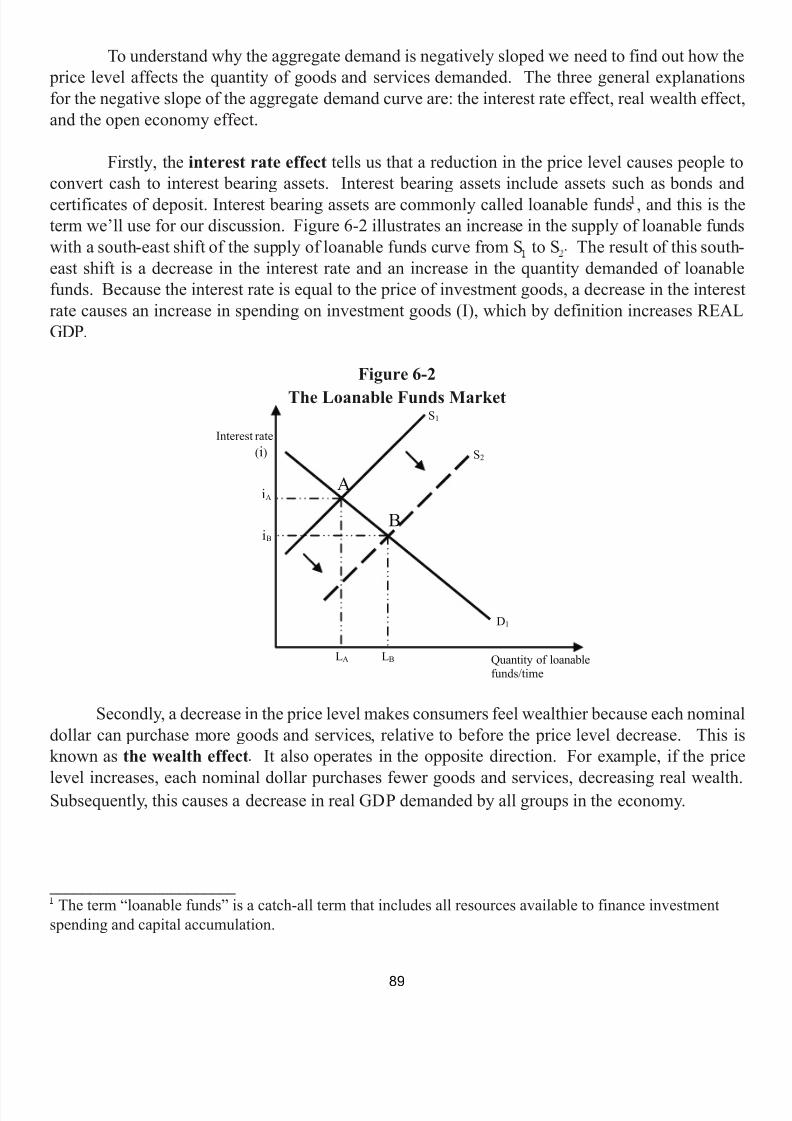
7/21/2019 PSU IVY Fundamentals of Economics
http://slidepdf.com/reader/full/psu-ivy-fundamentals-of-economics 91/118
To understand why the aggregate demand is negatively sloped we need to find out how the price level affects the quantity of goods and services demanded. The three general explanationsfor the negative slope of the aggregate demand curve are: the interest rate effect, real wealth effect,and the open economy effect.
Firstly, the interest rate effect tells us that a reduction in the price level causes people toconvert cash to interest bearing assets. Interest bearing assets include assets such as bonds andcertificates of deposit. Interest bearing assets are commonly called loanable funds , and this is theterm we’ll use for our discussion. Figure 6-2 illustrates an increase in the supply of loanable fundswith a south-east shift of the supply of loanable funds curve from S to S The result of this south-east shift is a decrease in the interest rate and an increase in the quantity demanded of loanablefunds. Because the interest rate is equal to the price of investment goods, a decrease in the interestrate causes an increase in spending on investment goods (I), which by definition increases REALGDP.
Figure 6-2The Loanable Funds Market
Secondly, a decrease in the price level makes consumers feel wealthier because each nominaldollar can purchase more goods and services, relative to before the price level decrease. This isknown as the wealth effect It also operates in the opposite direction. For example, if the price
level increases, each nominal dollar purchases fewer goods and services, decreasing real wealth.Subsequently, this causes a decrease in real GDP demanded by all groups in the economy.
_______________________ The term “loanable funds” is a catch-all term that includes all resources available to finance investment
spending and capital accumulation.
Interest rate(i)
Quantity of loanablefunds/time
D1
S1
S2
LA LB
iA
iB
A
B
89
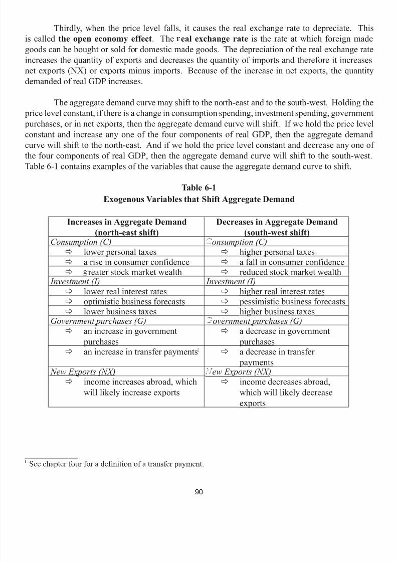
7/21/2019 PSU IVY Fundamentals of Economics
http://slidepdf.com/reader/full/psu-ivy-fundamentals-of-economics 92/118
Thirdly, when the price level falls, it causes the real exchange rate to depreciate. Thisis called the open economy effect . The eal exchange rate is the rate at which foreign madegoods can be bought or sold for domestic made goods. The depreciation of the real exchange rateincreases the quantity of exports and decreases the quantity of imports and therefore it increasesnet exports (NX) or exports minus imports. Because of the increase in net exports, the quantitydemanded of real GDP increases.
The aggregate demand curve may shift to the north-east and to the south-west. Holding the price level constant, if there is a change in consumption spending, investment spending, government purchases, or in net exports, then the aggregate demand curve will shift. If we hold the price levelconstant and increase any one of the four components of real GDP, then the aggregate demandcurve will shift to the north-east. And if we hold the price level constant and decrease any one ofthe four components of real GDP, then the aggregate demand curve will shift to the south-west.Table 6-1 contains examples of the variables that cause the aggregate demand curve to shift.
Table 6-1Exogenous Variables that Shift Aggregate Demand
Increases in Aggregate Demand(north-east shift)
Decreases in Aggregate Demand(south-west shift)
Consumption (C) onsumption (C)lower personal taxes higher personal taxes a rise in consumer confidence a fall in consumer confidence
reater stock market wealth reduced stock market wealth Investment (I) Investment (I)
lower real interest rates higher real interest rates optimistic business forecasts pessimistic business forecasts lower business taxes higher business taxes
Government purchases (G) overnment purchases (G) an increase in government
purchasesa decrease in government
purchasesan increase in transfer payments a decrease in transfer
payments New Exports (NX) ew Exports (NX)
income increases abroad, which
will likely increase exports
income decreases abroad,
which will likely decreaseexports
_____________ See chapter four for a definition of a transfer payment.
90
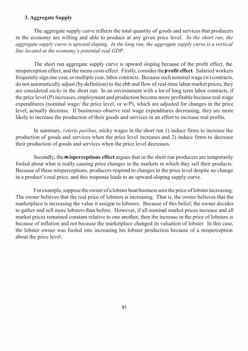
7/21/2019 PSU IVY Fundamentals of Economics
http://slidepdf.com/reader/full/psu-ivy-fundamentals-of-economics 93/118
3. Aggregate Supply
The aggregate supply curve reflects the total quantity of goods and services that producersin the economy are willing and able to produce at any given price level. In the short run, theaggregate supply curve is upward sloping. In the long run, the aggregate supply curve is a verticalline located at the economy’s potential real GDP.
The short run aggregate supply curve is upward sloping because of the profit effect, themisperception effect, and the menu costs effect. Firstly, consider the rofit effect Salaried workersfrequently sign one year, or multiple year, labor contracts. Because such nominal wage (w) contracts,do not automatically adjust (by definition) to the ebb and flow of real-time labor market prices, theyare considered sticky in the short run. In an environment with a lot of long term labor contracts, ifthe price level (P) increases, employment and production become more profitable because real wageexpenditures (nominal wage/ the price level, or w/P), which are adjusted for changes in the pricelevel, actually decrease. If businesses observe real wage expenditures decreasing, they are morelikely to increase the production of their goods and services in an effort to increase real profits.
In summary, eteris paribus , sticky wages in the short run 1) induce firms to increase the production of goods and services when the price level increases and 2) induce firms to decreasetheir production of goods and services when the price level decreases.
Secondly, the isperceptions effect argues that in the short run producers are temporarilyfooled about what is really causing price changes in the markets in which they sell their products.Because of these misperceptions, producers respond to changes in the price level despite no changein a product’s real price, and this response leads to an upward-sloping supply curve.
For example, suppose the owner of a lobster boat business sees the price of lobster increasing.The owner believes that the real price of lobsters is increasing. That is, the owner believes that themarketplace is increasing the value it assigns to lobsters. Because of this belief, the owner decidesto gather and sell more lobsters than before. However, if all nominal market prices increase and allmarket prices remained constant relative to one another, then the increase in the price of lobsters is
because of inflation and not because the marketplace changed its valuation of lobster. In this case,the lobster owner was fooled into increasing his lobster production because of a misperceptionabout the price level.
91
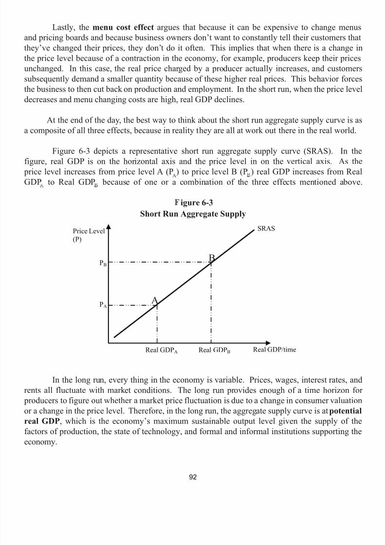
7/21/2019 PSU IVY Fundamentals of Economics
http://slidepdf.com/reader/full/psu-ivy-fundamentals-of-economics 94/118
Lastly, the menu cost effect argues that because it can be expensive to change menusand pricing boards and because business owners don’t want to constantly tell their customers thatthey’ve changed their prices, they don’t do it often. This implies that when there is a change inthe price level because of a contraction in the economy, for example, producers keep their pricesunchanged. In this case, the real price charged by a producer actually increases, and customerssubsequently demand a smaller quantity because of these higher real prices. This behavior forcesthe business to then cut back on production and employment. In the short run, when the price leveldecreases and menu changing costs are high, real GDP declines.
At the end of the day, the best way to think about the short run aggregate supply curve is asa composite of all three effects, because in reality they are all at work out there in the real world.
Figure 6-3 depicts a representative short run aggregate supply curve (SRAS). In thefigure, real GDP is on the horizontal axis and the price level in on the vertical axis. As the
price level increases from price level A (P A ) to price level B (P ) real GDP increases from RealGDP to Real GDP because of one or a combination of the three effects mentioned above.
igure 6-3Short Run Aggregate Supply
In the long run, every thing in the economy is variable. Prices, wages, interest rates, andrents all fluctuate with market conditions. The long run provides enough of a time horizon for producers to figure out whether a market price fluctuation is due to a change in consumer valuationor a change in the price level. Therefore, in the long run, the aggregate supply curve is at potentialreal GDP , which is the economy’s maximum sustainable output level given the supply of thefactors of production, the state of technology, and formal and informal institutions supporting theeconomy.
Real GDP/time
Price Level(P)
SRAS
A
BPB
PA
Real GDP A Real GDP B
92
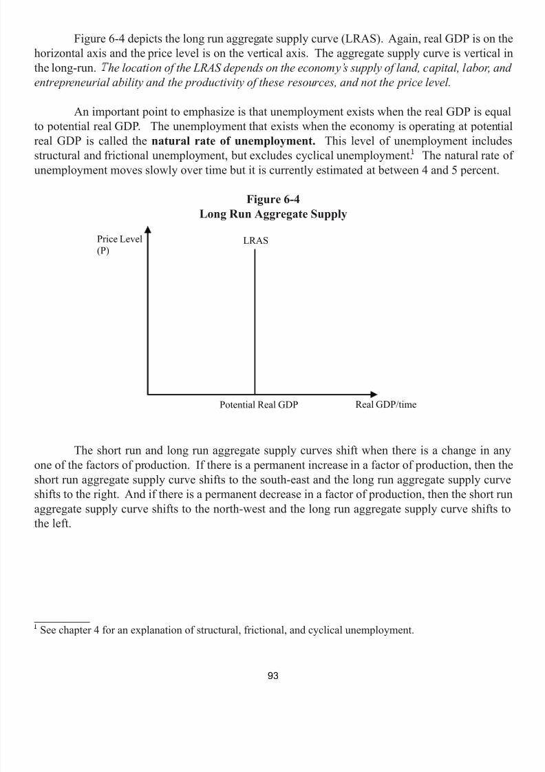
7/21/2019 PSU IVY Fundamentals of Economics
http://slidepdf.com/reader/full/psu-ivy-fundamentals-of-economics 95/118
Figure 6-4 depicts the long run aggregate supply curve (LRAS). Again, real GDP is on thehorizontal axis and the price level is on the vertical axis. The aggregate supply curve is vertical inthe long-run. he location of the LRAS depends on the economy’s supply of land, capital, labor, andentrepreneurial ability and the productivity of these resources, and not the price level.
An important point to emphasize is that unemployment exists when the real GDP is equalto potential real GDP. The unemployment that exists when the economy is operating at potentialreal GDP is called the natural rate of unemployment. This level of unemployment includesstructural and frictional unemployment, but excludes cyclical unemployment. The natural rate ofunemployment moves slowly over time but it is currently estimated at between 4 and 5 percent.
Figure 6-4Long Run Aggregate Supply
The short run and long run aggregate supply curves shift when there is a change in anyone of the factors of production. If there is a permanent increase in a factor of production, then theshort run aggregate supply curve shifts to the south-east and the long run aggregate supply curveshifts to the right. And if there is a permanent decrease in a factor of production, then the short runaggregate supply curve shifts to the north-west and the long run aggregate supply curve shifts tothe left.
__________ See chapter 4 for an explanation of structural, frictional, and cyclical unemployment.
Real GDP/time
Price Level(P)
LRAS
Potential Real GDP
93
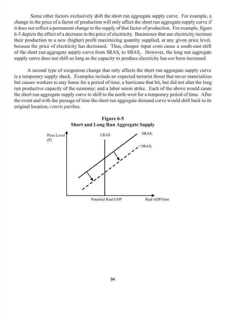
7/21/2019 PSU IVY Fundamentals of Economics
http://slidepdf.com/reader/full/psu-ivy-fundamentals-of-economics 96/118
Some other factors exclusively shift the short run aggregate supply curve. For example, achange in the price of a factor of production will only affect the short run aggregate supply curve ifit does not reflect a permanent change in the supply of that factor of production. For example, figure6-5 depicts the effect of a decrease in the price of electricity. Businesses that use electricity increasetheir production to a new (higher) profit maximizing quantity supplied, at any given price level,
because the price of electricity has decreased. Thus, cheaper input costs cause a south-east shiftof the short run aggregate supply curve from SRAS to SRAS However, the long run aggregatesupply curve does not shift so long as the capacity to produce electricity has not been increased.
A second type of exogenous change that only affects the short run aggregate supply curveis a temporary supply shock. Examples include an expected terrorist threat that never materializes
but causes workers to stay home for a period of time; a hurricane that hit, but did not alter the longrun productive capacity of the economy; and a labor union strike. Each of the above would causethe short run aggregate supply curve to shift to the north-west for a temporary period of time. Afterthe event and with the passage of time the short run aggregate demand curve would shift back to itsoriginal location, eteris paribus
Figure 6-5Short and Long Run Aggregate Supply
Real GDP/time
Price Level(P)
SRAS 1
Potential Real GDP
SRAS 2
LRAS
94

7/21/2019 PSU IVY Fundamentals of Economics
http://slidepdf.com/reader/full/psu-ivy-fundamentals-of-economics 97/118
Table 6-2 contains examples of the factors that cause the short run aggregate supply and thelong run aggregate supply curve to shift. Again, hese factors shift both the long run and short runaggregate supply only if the effect is permanent. If the effect is not permanent, then only the shortrun aggregate supply curve will shift.
Table 6-2xogenous Variables that Shift Aggregate Supply
An increase in Aggregate Supply(SRAS: south-east shift)(LRAS: rightward shift)
A decrease in Aggregate Supply(SRAS: north-west shift)(LRAS: leftward shift)
Lower costs Higher costslower wages higher wagesother input prices fall other input prices rise
Government Policy higher oil prices tax cuts overnment Policy
deregulation tax increaseslower trade barriers overregulation
Economic growth higher trade barriers improvements in technology A decline in labor productivity
productivity advances errorist Attacksan increase in labor atural Disasters
Favorable weather Unfavorable weather
95
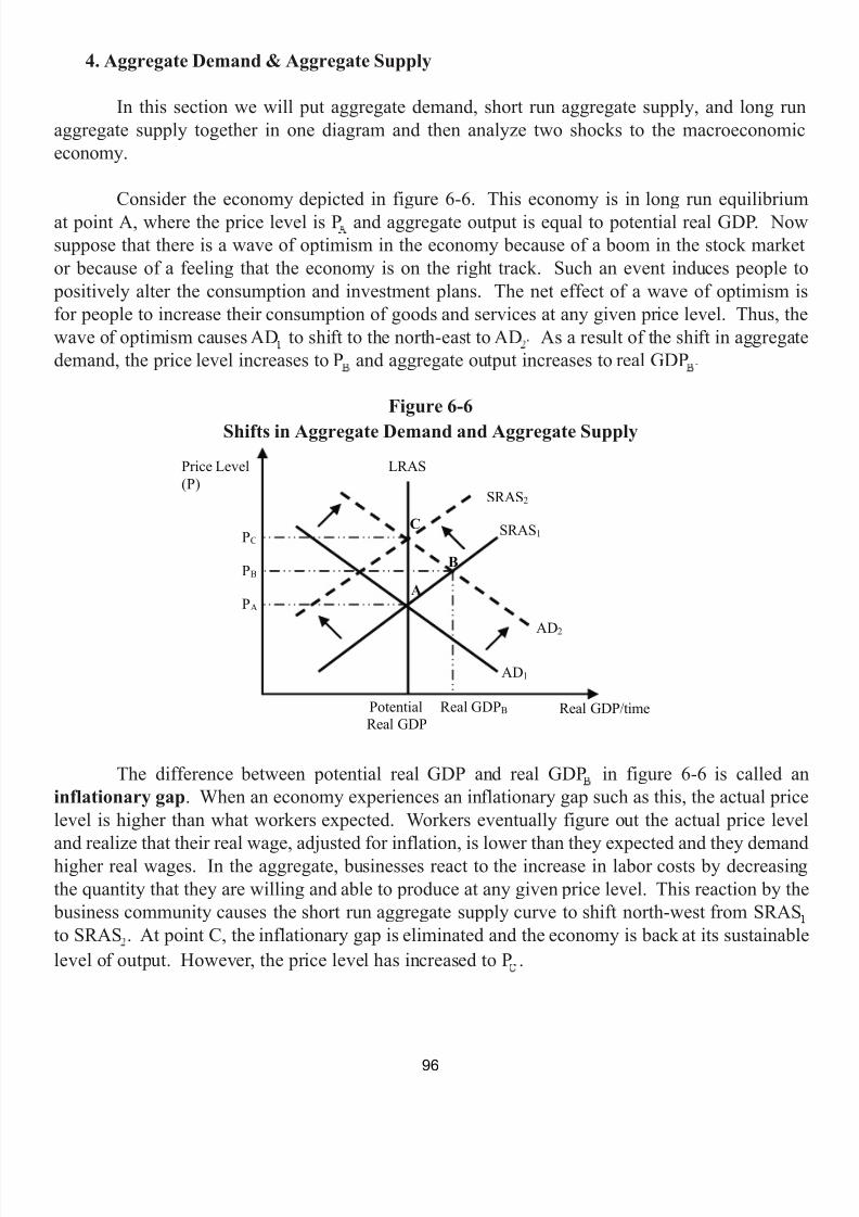
7/21/2019 PSU IVY Fundamentals of Economics
http://slidepdf.com/reader/full/psu-ivy-fundamentals-of-economics 98/118

7/21/2019 PSU IVY Fundamentals of Economics
http://slidepdf.com/reader/full/psu-ivy-fundamentals-of-economics 99/118
Now consider figure 6-7, which is an economy in long run equilibrium at point C with a pricelevel equal to P and aggregate output equal to potential real GDP. Suppose a wave of pessimismwashes over the economy, lowering consumer confidence and decreasing the quantity of goods andservices that consumers demand at any given price level. As a result, AD shifts south-west to ADThe short run equilibrium is now at point B, where the price level is P and aggregate output is atreal GDP
The difference between potential real GDP and real GDP in figure 6-7 is called a deflationarygap An economy that is in a deflationary gap experiences an unemployment rate that is higherthan the natural rate of unemployment. This is the case because cyclical unemployment is nowadded to the natural rate of unemployment.
The economy will eventually self-correct and eliminate a deflationary gap. For example, because of the higher than natural rates of unemployment, workers are willing to accept lowerwages in an effort to get a job. In the aggregate, businesses experience lower input costs and asa result they increase their profit maximizing quantity supplied at every given price level. Thisis demonstrated in figure 6-7 with a south-east shift of the short run aggregate supply curve fromSRAS to SRAS Long run equilibrium is again reached at point A. At this point, the price levelequals P , the recessionary gap is eliminated, and the economy is again operating at potential realGDP.
Figure 6-7Shifts in Aggregate Demand and Aggregate Supply
_____________ See Chapter 4 for a definition of cyclical unemployment.
Real GDP/time
Price Level(P)
AD 2
Real GDP B PotentialReal GDP
SRAS 2
LRAS
AD 1
C
B
PB
PA
SRAS 1
A
PC
97
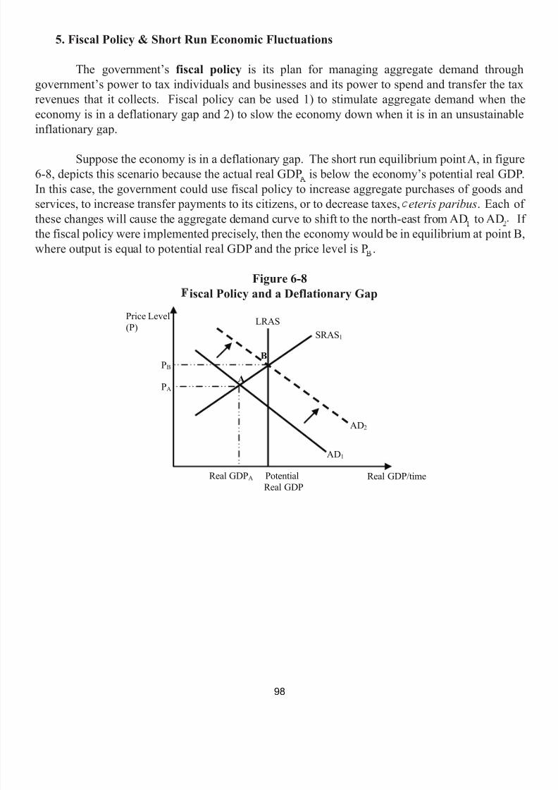
7/21/2019 PSU IVY Fundamentals of Economics
http://slidepdf.com/reader/full/psu-ivy-fundamentals-of-economics 100/118
5. Fiscal Policy & Short Run Economic Fluctuations
The government’s fiscal policy is its plan for managing aggregate demand throughgovernment’s power to tax individuals and businesses and its power to spend and transfer the taxrevenues that it collects. Fiscal policy can be used 1) to stimulate aggregate demand when theeconomy is in a deflationary gap and 2) to slow the economy down when it is in an unsustainableinflationary gap.
Suppose the economy is in a deflationary gap. The short run equilibrium point A, in figure6-8, depicts this scenario because the actual real GDP is below the economy’s potential real GDP.In this case, the government could use fiscal policy to increase aggregate purchases of goods andservices, to increase transfer payments to its citizens, or to decrease taxes, eteris paribus . Each ofthese changes will cause the aggregate demand curve to shift to the north-east from AD to AD Ifthe fiscal policy were implemented precisely, then the economy would be in equilibrium at point B,where output is equal to potential real GDP and the price level is P .
Figure 6-8iscal Policy and a Deflationary Gap
Real GDP/time
Price Level(P)
AD 1
Real GDP A PotentialReal GDP
LRAS
AD 2
B
A
PA
SRAS 1
PB
98
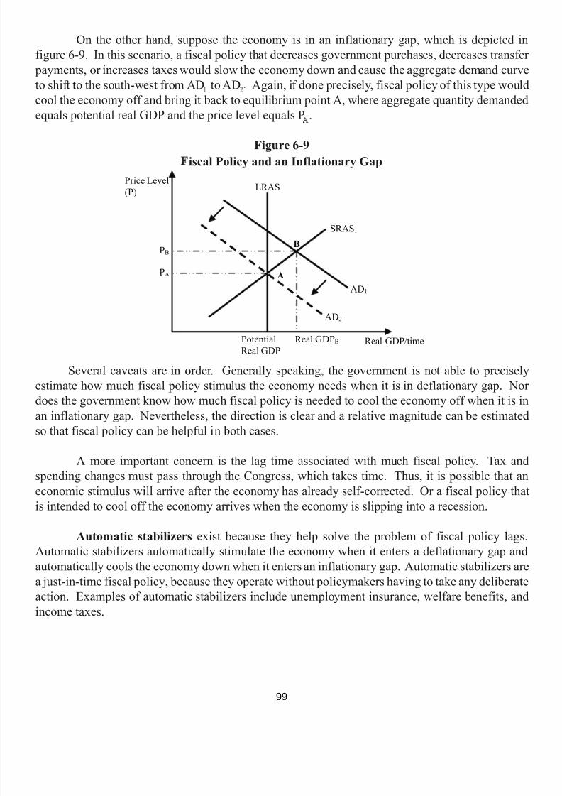
7/21/2019 PSU IVY Fundamentals of Economics
http://slidepdf.com/reader/full/psu-ivy-fundamentals-of-economics 101/118
On the other hand, suppose the economy is in an inflationary gap, which is depicted infigure 6-9. In this scenario, a fiscal policy that decreases government purchases, decreases transfer
payments, or increases taxes would slow the economy down and cause the aggregate demand curveto shift to the south-west from AD to AD Again, if done precisely, fiscal policy of this type wouldcool the economy off and bring it back to equilibrium point A, where aggregate quantity demandedequals potential real GDP and the price level equals P .
Figure 6-9iscal Policy and an Inflationary Gap
Several caveats are in order. Generally speaking, the government is not able to preciselyestimate how much fiscal policy stimulus the economy needs when it is in deflationary gap. Nordoes the government know how much fiscal policy is needed to cool the economy off when it is in
an inflationary gap. Nevertheless, the direction is clear and a relative magnitude can be estimatedso that fiscal policy can be helpful in both cases.
A more important concern is the lag time associated with much fiscal policy. Tax andspending changes must pass through the Congress, which takes time. Thus, it is possible that aneconomic stimulus will arrive after the economy has already self-corrected. Or a fiscal policy thatis intended to cool off the economy arrives when the economy is slipping into a recession.
Automatic stabilizers exist because they help solve the problem of fiscal policy lags.Automatic stabilizers automatically stimulate the economy when it enters a deflationary gap andautomatically cools the economy down when it enters an inflationary gap. Automatic stabilizers area just-in-time fiscal policy, because they operate without policymakers having to take any deliberateaction. Examples of automatic stabilizers include unemployment insurance, welfare benefits, andincome taxes.
Real GDP/time
Price Level(P)
AD 2
Potential Real GDP B Real GDP
LRAS
AD 1
B PB
PA
SRAS 1
A
99

7/21/2019 PSU IVY Fundamentals of Economics
http://slidepdf.com/reader/full/psu-ivy-fundamentals-of-economics 102/118
6. Monetary Policy & Short Run Economic Fluctuations
Monetary policy is any action that changes the supply of money and alters the interestrate. In the United States, monetary policy is implemented by the Federal Reserve System.
Figure 6-10 depicts a new model of the money market (one that is different from the model presented in chapter 5) that is helpful in showing the effects of monetary policy changes. In thismodel, the interest rate is on the vertical axis and the quantity of money is on the horizontal axis.The money supply curve (MS) is vertical because it is determined by the Federal Reserve. Themoney demand curve (MD) is downward sloping. This is the case because as the interest rateincreases, the opportunity cost of holding money increases and the quantity demanded of moneydecreases. Also, as the interest rate decreases, the opportunity cost of holding money decreases and
people choose to increase there quantity demanded of money. The equilibrium interest rate is theinterest rate that balances the quantity demanded and quantity supplied of money.
Figure 6-10The Money Market
Assume that the money market is in equilibrium where the equilibrium interest rate is iand the equilibrium quantity of money is Q Suppose that the Federal Reserve increases the moneysupply from MS to MS by implementing one or several of its three monetary tools (see chapter 5for a discussion of monetary tools). An increase in the money supply would cause a decrease in theinterest rate from i to i and an increase in the equilibrium quantity of money from Q to Q . If theFederal Reserve subsequently decreased the money supply from MS to MS , then the interest ratewould increase back to i and the equilibrium quantity of money would decrease back to Q
Quantity of Money/time
Interest Rate(i)
MD 1
Q1 Q2
MS 2 MS 1
i1
i2
100
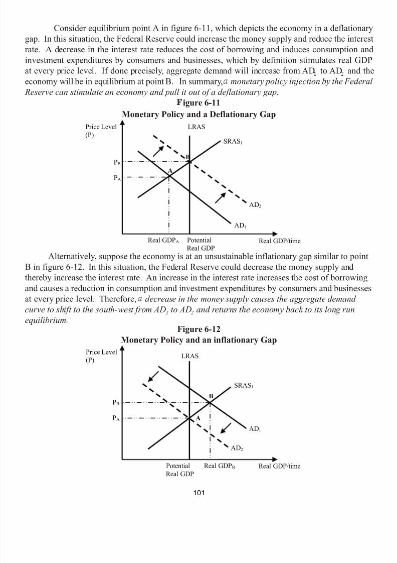
7/21/2019 PSU IVY Fundamentals of Economics
http://slidepdf.com/reader/full/psu-ivy-fundamentals-of-economics 103/118
Consider equilibrium point A in figure 6-11, which depicts the economy in a deflationarygap. In this situation, the Federal Reserve could increase the money supply and reduce the interestrate. A decrease in the interest rate reduces the cost of borrowing and induces consumption andinvestment expenditures by consumers and businesses, which by definition stimulates real GDPat every price level. If done precisely, aggregate demand will increase from AD to AD and theeconomy will be in equilibrium at point B. In summary, monetary policy injection by the Federal
Reserve can stimulate an economy and pull it out of a deflationary gap .igure 6-11
Monetary Policy and a Deflationary Gap
Alternatively, suppose the economy is at an unsustainable inflationary gap similar to pointB in figure 6-12. In this situation, the Federal Reserve could decrease the money supply andthereby increase the interest rate. An increase in the interest rate increases the cost of borrowingand causes a reduction in consumption and investment expenditures by consumers and businessesat every price level. Therefore, decrease in the money supply causes the aggregate demandcurve to shift to the south-west from AD to AD and returns the economy back to its long runequilibrium
Figure 6-12Monetary Policy and an inflationary Gap
Real GDP/time
Price Level(P)
AD 1
Real GDP A PotentialReal GDP
LRAS
AD 2
B
A
PA
SRAS 1
PB
Real GDP/time
Price Level(P)
AD 2
Potential Real GDP B Real GDP
LRAS
AD 1
B
PB
PA
SRAS 1
A
101

7/21/2019 PSU IVY Fundamentals of Economics
http://slidepdf.com/reader/full/psu-ivy-fundamentals-of-economics 104/118
Glossary
1. the factors of production - The factors of production encompass all the possible productiveresources used to produce goods and services. Labor, capital, land, and entrepreneurial ability areexamples of factors of production.
2. opportunity cost - The opportunity cost of something is what you give up to get it.
3. production possibilities frontier - A production possibilities frontier is a model of a two-goodeconomy that shows how much the economy can produce using all of its factors of productionefficiently.
4. increasing opportunity cost - As more and more of an economy’s factors of production areemployed in the production of a good, the economy must sacrifice the production of other goods atan increasing rate.
5. absolute advantage - To have an absolute advantage in something means that one has the lowestabsolute production cost relative to those with whom they are compared.
6. comparative advantage - To have a comparative advantage in something means that one hasthe lowest opportunity cost relative to those with whom they are compared.
Cha ter 2
1. a demand schedule - A table showing the relationship between price and the quantity of a goodthat buyers are willing to buy.
2. a demand curve - A demand curve is a picture of the way an individual responds to changing prices of a good.
3. a demand function - A relationship between independent demand variables, such as the priceof good X and the price of a substitute good Y, and the dependent variable, the quantity demandedof good X.
4. the law of demand - As the price of a good increases, ceteris paribus, the quantity demanded ofthe good decreases.
5. he market demand curve - The horizontal summation of individual demand curves yields themarket demand curve.
6. the market demand schedule - The market demand schedule is a table that is calculated bysumming up how many units of a good buyers are willing to purchase at every market price.
102
7/21/2019 PSU IVY Fundamentals of Economics
http://slidepdf.com/reader/full/psu-ivy-fundamentals-of-economics 105/118
7. the price elasticity of demand - A measure of the relationship between a percentage change inthe market price of product and a consequential percentage change in the quantity demanded of a
product.
8. the cross price elasticity of demand - A measure of the relationship between a percentagechange in the market price of product X and a consequential percentage change in the quantitydemanded of product Y.
9. the income elasticity of demand - A measure of the relationship between a percentage changein income and a consequential percentage change in the quantity demanded of a product.
10. a supply schedule - A table showing the relationship between price and the quantity of a goodthat sellers are willing to produce.
11. a supply curve - A supply curve is a picture of the way in which a producer responds tochanging market prices of a good.
12. a supply function - A relationship between independent supply variables, such as the price ofinputs and technology, and the dependent variable, the quantity supplied of a good.
13. the law of supply - As the price of a good increases, ceteris paribus, the quantity supplied ofthe good increases.
14. he market supply curve - The horizontal summation of individual supply curves yields themarket supply curve.
15. he market supply schedule - The market supply schedule is calculated by summing up how
many units of a good sellers are willing to produce at every market price.
16. the elasticity of supply - A measure of the relationship between a percentage change in themarket price of a product and a consequential percentage change in the quantity supplied of a
product.
17. arket equilibrium - An economic balance in which no individual would be better off doingsomething different; an equality of supply and demand.
18. comparative-static analysis - The process of comparing two market equilibrium (static) points,
one equilibrium point before and the other after a change in an independent variable.
103

7/21/2019 PSU IVY Fundamentals of Economics
http://slidepdf.com/reader/full/psu-ivy-fundamentals-of-economics 106/118
Chapter 31. the short run - The short run is a time horizon within which a business is unable to adjust atleast one input. In other words, in the short run there exists some fixed cost.
2. the long run - The long run is a time horizon long enough for the seller to adjust all inputs.Thus, if you observe a business with no fixed costs, then it is in a long run state.
3. fixed costs - Costs that do not vary with changes in the quantity produced are called fixedcosts.
4. ariable costs - Costs that do vary with changes in the quantity produced are called variablecosts.
5. total costs - The sum of fixed costs and variable costs.
6. average fixed costs - Average fixed cost equals fixed cost divided by the quantity produced.
7. average variable costs - Average variable cost equals the variable cost divided by the quantity produced.
8. average total costs - Average total cost equals the total cost divided by the quantity produced orit is the sum of average fixed cost plus average variable cost.
9. arginal costs - Marginal cost is equal to the change in the total cost that arises from an extraunit of production. It is calculated by taking the change in total cost and dividing it by the changein the quantity produced.
10. sunk costs - A cost that has already been committed and cannot be recovered.
11. total revenue - Total revenue is calculated by multiplying price and quantity.
12. marginal revenue - Marginal Revenue is the change in total revenue generated from anadditional unit sold. It is calculated by taking the change in total revenue divided by the change inquantity sold.
13. erfect competition - An industry with many buyers and many sellers. An industry in whichthe good is homogeneous. And it is an industry in which all who want to enter the industry are free
to do so and any business may exit at a time of their choosing.
14. onopoly - An industry controlled by a monopolist. A monopolist is a firm that is theonly seller of a good. The good the monopolist sells is heterogeneous. And the market that themonopolist sells its product in has barriers to entry.
15. the profit maximizing rule - The profit maximizing rule states that a business maximizes profits when it produces where the marginal revenue from selling another unit equals marginalcost of producing an additional unit.
104
7/21/2019 PSU IVY Fundamentals of Economics
http://slidepdf.com/reader/full/psu-ivy-fundamentals-of-economics 107/118
16. the shut down rule - A business should shut down if production at the profit maximizingquantity (where MR=MC) generates total revenues that are less than variable costs, in all othercases the business should stay open.
17. economies of scale - A range of production in which average total costs decline as outputincreases.
18. diseconomies of scale - A range of output in which average total costs increase as outputincreases.
19. constant economies of scale - A range of production where average total costs remain constantas output increases.
20. joint costs - Costs that do not change with changes in the scope of production.
21. economies of scope - When an organization can produce several products together at less costthan could a group of single product firms operating independently.
Cha ter 4
1. nominal gross domestic product - The market value of final goods and services produced atcurrent year prices.
2. the business cycle - Fluctuations in economic activity, such as employment and real GDP.
3. real gross domestic product - A measure of the market value of the production of final goodsand services, controlling changes in the price level.
4. transfer payments - Transfer payments are a sum of money that the government gives to certainindividuals as outright grants. Examples of a transfer payment include a social security payment,a welfare benefit, and unemployment insurance benefit.
5. he national income identity - The accounting concept which states that, in a time period,aggregate expenditure on wages, interest, rents, and profits is equal to nominal GDP is equal to
consumption spending, investment spending, government spending, and net exports.
6. the circular flow - The cycle depicted in the circular flow diagram graphically depicts thenational income identity.
7. the consumer price index - The consumer price index (CPI) measures changes over timein the cost of buying a “market basket” of goods and services purchased by a typical family.
105
7/21/2019 PSU IVY Fundamentals of Economics
http://slidepdf.com/reader/full/psu-ivy-fundamentals-of-economics 108/118
9. the inflation rate - A percentage change in a price index between two periods.
10. he unemployment rate - The unemployment rate is defined as the percent of people who dowant a job right now, have been looking for work, but have not found a job that they would takedivided by the labor force.
11. he labor force - The sum of people that have a job and those that are actively seeking a job.
12. discouraged workers - People who have tried to find a job for a long period of time and cannot find a job. They are frustrated in their search and have stopped looking for work.
13. the types of unemployment - Frictional unemployment (which occurs because it takes timefor workers to search for the jobs that best suit their tastes and job skills), structural unemployment(which occurs because the number of jobs available in a labor market is insufficient to provide
jobs for all that want a job), and cyclical unemployment (which occurs because of declines in theeconomy’s aggregate output during economic contractions and recessions).
Cha ter 5
1. the functions of money - The three basic functions of money are a medium of exchange, a storeof value, and a unit-of-account. Money is a medium of exchange because money makes exchangeeasier. Money is also a store of value. People will hold money only if they believe it will continueto have some value, so money can operate as a medium of exchange only if it serves as a store ofvalue. Lastly, money is a unit-of-account. Money is a convenient and widely recognized measurefor accounting and transactions; it is a yardstick for measuring the value of all goods and services.
2. the types of money - Paper money that has no intrinsic value, e.g., the U.S. dollar, is knownas fiat money. Fiat money is paper money that derives its status as money from the power of thestate, or by fiat. It is money because the government says that it is money, it otherwise has no realvalue. Fiat money can be contrasted with commodity money, which exists when some intrinsicallyvaluable good also serves as money. Gold is an example of commodity money because it has valueeven if it were not used as money.
3. classifications of the money supply - The most narrowly defined money supply is M1, whichincludes currency, traveler’s checks, demand deposits, and other checkable deposits. M2 is more
expansive. It includes everything in M1, plus savings deposits, small time deposits, money marketmutual funds, and a few other minor categories.
4. he money creation process - A process that describes the amount of money the banking systemcreates with each dollar held in reserve.
106

7/21/2019 PSU IVY Fundamentals of Economics
http://slidepdf.com/reader/full/psu-ivy-fundamentals-of-economics 109/118
5. bank reserves - Deposits that a bank has received but has not loaned out.
6. required reserve deposit ratio - Bank reserves divided by checkable deposits.
7. the Federal Reserve Bank - The central bank of the United States.
8. onetary policy - The setting of the money supply by policymakers at the central bank. Thecentral bank, e.g., the Federal Reserve Bank in the U.S., has three tools at its disposal to alter themoney supply: open market operations, reserve requirement changes, and changes to the FederalReserve’s discount rate.
9. the price level - A measure of the cost of a typical market basket. Measures of the price levelare the consumer price index and the producer price index. As the overall level of prices increases,the value of a unit of money decreases.
10. the value of money - The quantity of real goods and services that each nominal unit of moneycan purchase.
11. oney supply - The quantity of money available in the economy.
12. oney demand - A relationship between independent variables such as the interest rate andthe price level and the dependent variable quantity demanded of money. For example, as the pricelevel increases, ceteris paribus, the quantity demanded of money decreases.
Cha ter 6
1. classical dichotomy - In the long run, we assume that there is a separation of real (adjusted for price level changes) and nominal (not adjusted for price level changes) variables. This separationof real and nominal variables is a concept that is formally called the classical dichotomy.
2. monetary neutrality - A concept that in the long run, the money supply affects only nominalvariables and not real variables. This is demonstrated in chapter five’s figure 5-2, where a changein the money supply by the Federal Reserve strictly causes the price level to change, i.e., it causesinflation or deflation, and it has no effect on the real value people place on goods and services.
3. aggregate demand - The aggregate demand curve reflects the real gross domestic productdemanded by all groups in the economy at any given price level.
107
7/21/2019 PSU IVY Fundamentals of Economics
http://slidepdf.com/reader/full/psu-ivy-fundamentals-of-economics 110/118
4. the interest rate effect - The interest rate effect tells us that a reduction in the price level causes people to convert cash to interest bearing assets. An increase in the supply of loanable funds causesa south-east shift of the supply of loanable funds, which leads to a lower interest rate. Becausethe interest rate is equal to the price of investment goods, a decrease in the interest rate causes anincrease in spending on investment goods (I), which by definition increases real GDP
5. the wealth effect - A decrease in the price level makes consumers feel wealthier because eachnominal dollar can purchase more goods and services, relative to before the price level decrease.This causes an increase in real GDP demanded at every price level.
6. the open economy effect - When the price level falls, it causes the real exchange rate todepreciate. The real exchange rate is the rate at which foreign made goods can be bought or sold fordomestic made goods. The depreciation of the real exchange rate increases the quantity of exportsand decreases the quantity of imports and therefore it increases net exports (NX) or exports minusimports. Because of the increase in net exports, the quantity demanded of real GDP increases.
7. the real exchange rate - The real exchange rate is the rate at which foreign made goods can be bought or sold for domestic made goods.
8. he short run aggregate supply - The aggregate supply curve reflects the total quantity ofgoods and services that producers in the economy are willing and able to produce at any given
price level. The short run aggregate supply curve is upward sloping because of the profit effect, themisperception effect, and the menu costs effect.
9. the profit effect – The concept that, ceteris paribus, sticky wages in the short run 1) induce firms
to increase the production of goods and services when the price level increases and 2) induce firmsto decrease their production of goods and services when the price level decreases because it leadsto an increase in real profits.
10. the misperceptions effect - The misperceptions effect argues that in the short run producersare temporarily fooled about what is really causing price changes in the markets in which they selltheir products. Because of these misperceptions, producers respond to changes in the price leveldespite no change in a product’s real price, and this response leads to an upward-sloping supplycurve.
11. the menu costs effect - The menu cost effect argues that because it can be expensive to changemenus and pricing boards and because business owners don’t want to constantly tell their customersthat they’ve changed their prices, they don’t do it often. This implies that when there is a changein the price level because of a contraction in the economy, for example, producers keep their pricesunchanged.
108
7/21/2019 PSU IVY Fundamentals of Economics
http://slidepdf.com/reader/full/psu-ivy-fundamentals-of-economics 111/118
12. long run aggregate supply - The aggregate supply curve is vertical in the long-run. Thelocation of the long run aggregate supply curve depends on the economy’s supply of land, capital,labor, and entrepreneurial ability and the productivity of these resources, and not the price level.
13. potential real GDP - The economy’s maximum sustainable output level given the supply ofthe factors of production, the state of technology, and formal and informal institutions supportingthe economy.
14. the natural rate of unemployment - The unemployment that exists when the economy isoperating at potential real GDP is called the natural rate of unemployment.
15. inflationary gap - The inflationary gap is the amount by which the equilibrium level of realGDP exceeds potential real GDP.
16. deflationary gap - The deflationary gap is the amount by which the equilibrium level of realGDP falls short of potential real GDP.
17. fiscal policy - The government’s fiscal policy is its plan for managing aggregate demandthrough government’s power to tax individuals and businesses and its power to spend and transferthe tax revenues that it collects.
18. automatic stabilizer - Automatic stabilizers automatically stimulate the economy when it entersa deflationary gap and automatically cools the economy down when it enters an inflationary gap.Automatic stabilizers are a just-in-time fiscal policy, because they operate without policymakershaving to take any deliberate action. Examples of automatic stabilizers include unemployment
insurance, welfare benefits, and income taxes.
19. monetary policy - Monetary policy is any action that changes the supply of money. In theUnited States, monetary policy is implemented by the Federal Reserve System.
109
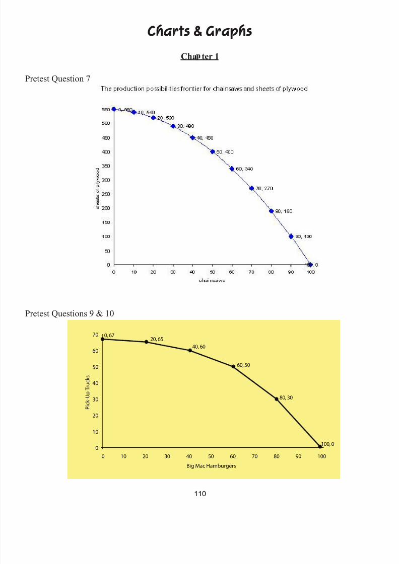
7/21/2019 PSU IVY Fundamentals of Economics
http://slidepdf.com/reader/full/psu-ivy-fundamentals-of-economics 112/118
Charts & GraphsCha ter 1
Pretest Question 7
Pretest Questions 9 & 10
�
�
�
�
�
�
�
�
� �
�
�
�
�
�
110
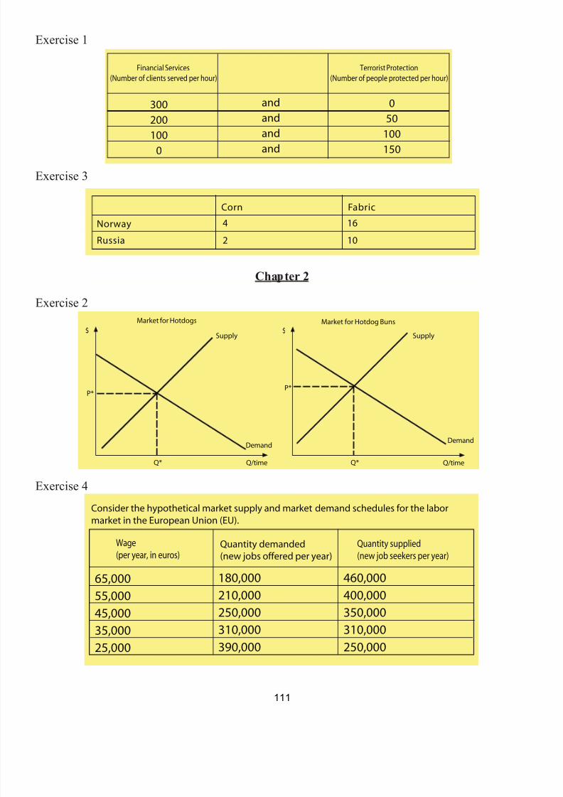
7/21/2019 PSU IVY Fundamentals of Economics
http://slidepdf.com/reader/full/psu-ivy-fundamentals-of-economics 113/118
Exercise 1
Exercise 3
Cha ter 2
Exercise 2
Exercise 4
�
�
�
��
��
��
�
�
�
��
�
� �
�
�
�
�
111
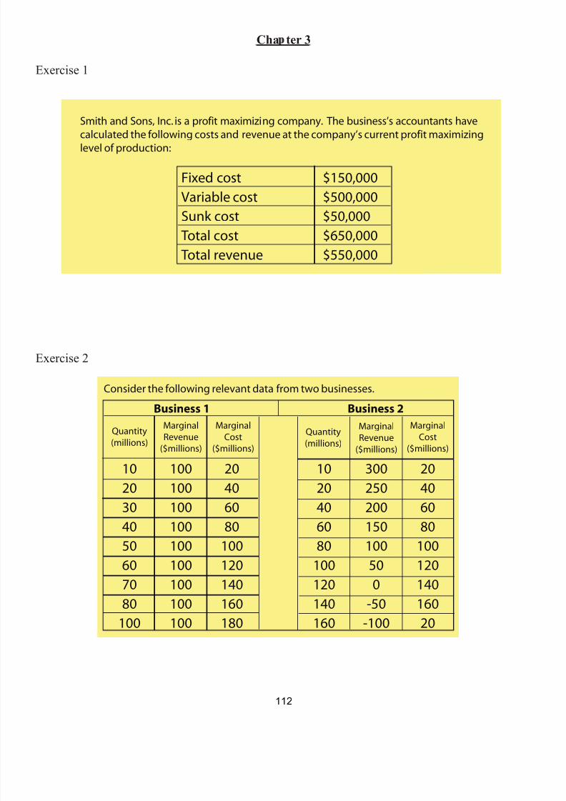
7/21/2019 PSU IVY Fundamentals of Economics
http://slidepdf.com/reader/full/psu-ivy-fundamentals-of-economics 114/118
Cha ter 3
Exercise 1
Exercise 2
� � � �
�
�
�
�
�
�
112
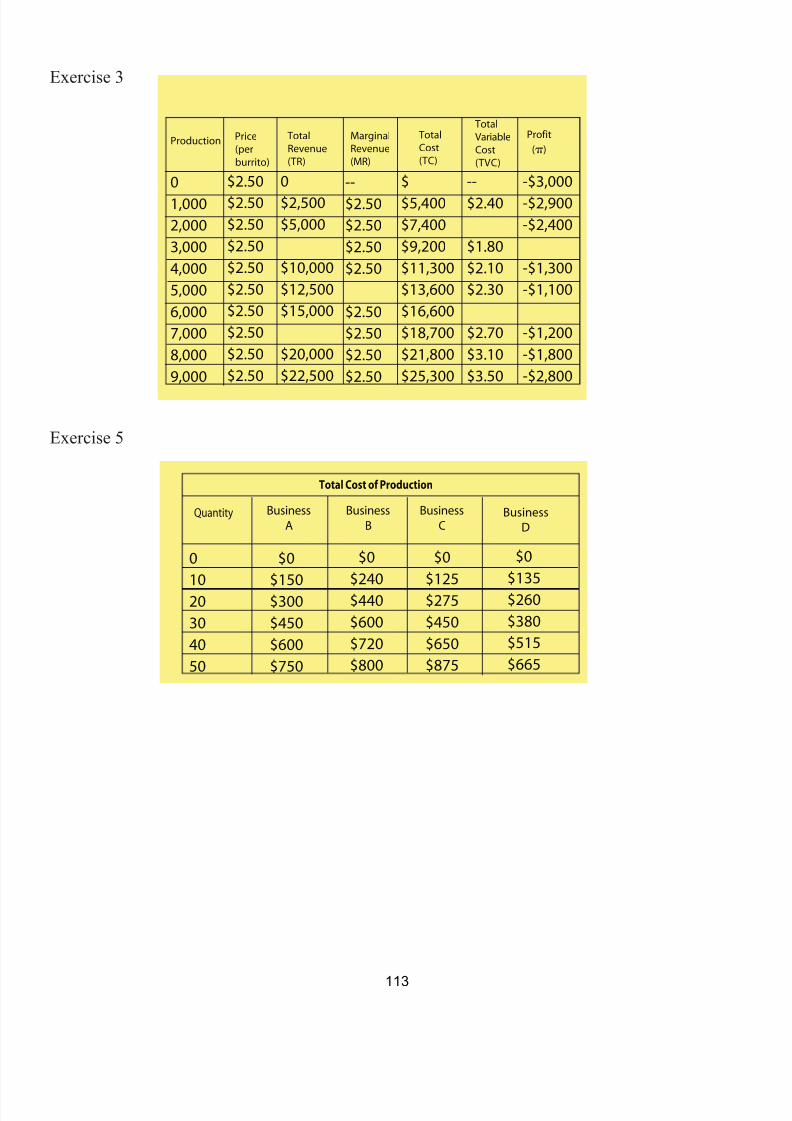
7/21/2019 PSU IVY Fundamentals of Economics
http://slidepdf.com/reader/full/psu-ivy-fundamentals-of-economics 115/118
Exercise 3
Exercise 5
�
�
�
�
�
�
�
�
�
�
�
�
�
�
�
�
�
�
�
�
�
�
�
�
�
�
�
�
�
�
�
�
�
�
�
�
�
�
�
�
p
�
�
�
�
�
�
�
�
�
�
�
�
�
�
�
�
�
�
�
�
�
�
�
�
�
�
�
�
�
�
�
�
�
�
�
�
113
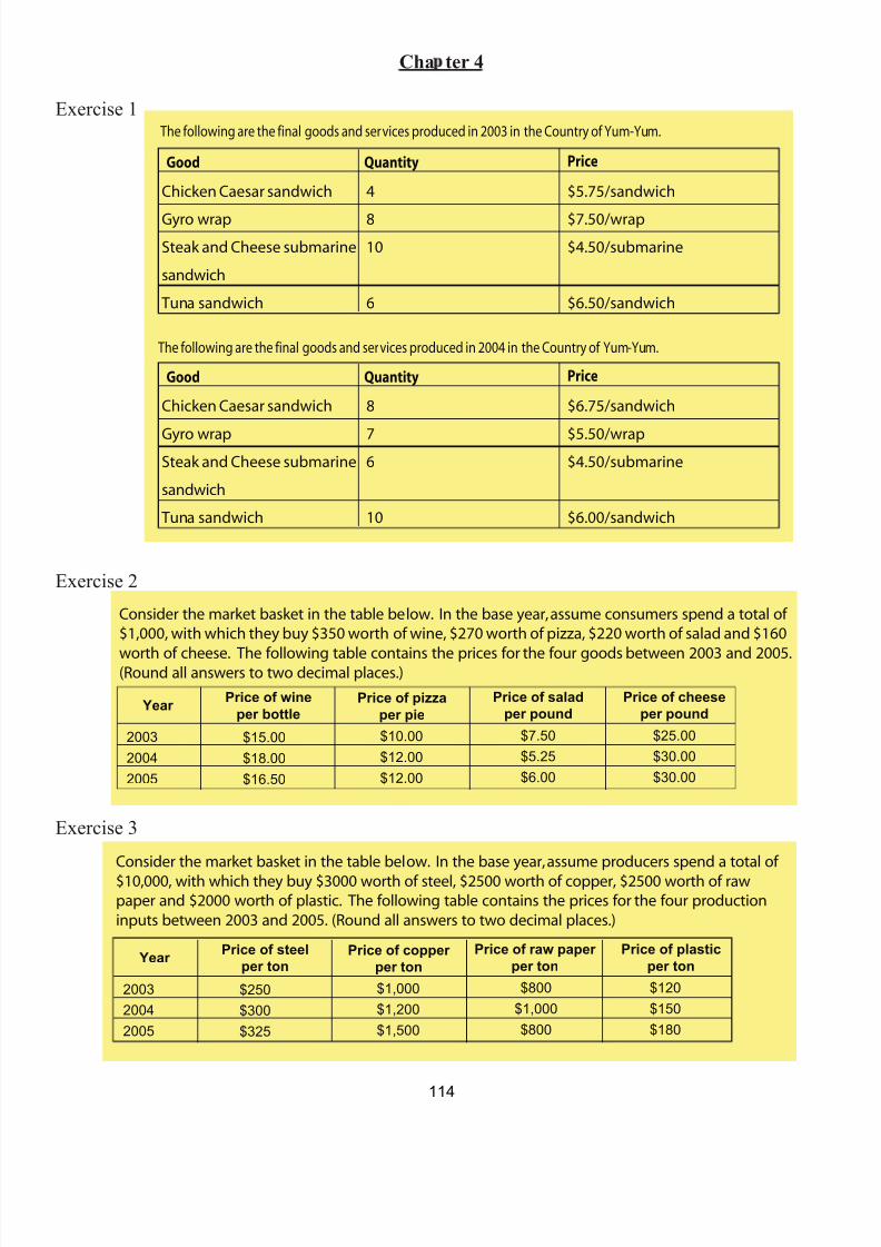
7/21/2019 PSU IVY Fundamentals of Economics
http://slidepdf.com/reader/full/psu-ivy-fundamentals-of-economics 116/118
Cha ter 4
Exercise 1
Exercise 2
Exercise 3
�
�
�
�
�
�
�
�
�
�
Price of wineper bottle
2003
2004
2005
$10.00
$12.00
$12.00
Price of pizzaper pie
Price of saladper pound
$7.50
$5.25
$6.00
Year
$15.00
$18.00
$16.50
� � � �
Price of cheeseper pound
$25.00
$30.00
$30.00
Price of steelper ton
20032004
2005
$1,000$1,200
$1,500
Price of copper per ton
Price of raw paper per ton
$800
$1,000
$800
Year
$250$300
$325
� � � �
�
Price of plasticper ton
$120
$150
$180
114

7/21/2019 PSU IVY Fundamentals of Economics
http://slidepdf.com/reader/full/psu-ivy-fundamentals-of-economics 117/118
Exercise 4
Cha ter 5
Exercise 2
�
�
�
Government bondsCurrency (=bank reserves)
Loans
Balance sheet of the Bank of Boston
�
�
�
�
115

7/21/2019 PSU IVY Fundamentals of Economics
http://slidepdf.com/reader/full/psu-ivy-fundamentals-of-economics 118/118
Cha ter 6
Exercise 4
Exercise 5
Real GDP/time
Price Level(P)
AD 1
Real GDP D Potential Real GDP B
Real GDP
SRAS 1
LRAS
AD 2
A
B PB
PA
SRAS 2
C PC
D
�
� � � � � � �
� � � � �
Price Level(P)
SRAS 1
LRAS
SRAS 2
C PC