Provisioning Cloud-Based Computing Resourcesvia a Dynamical Systems Approach

Marty Kandes

University of California, San Diego

May 18, 2016

Objective

Build a service for provisioning cloud-based computing resourcesthat can be used to augment users’ existing, fixed resources andmeet their batch job demands.

Vision

AWS

CM

SN

WN

CMOSG

OSG

AWS

WN

WN

LOCAL LOCAL

condor annex = HTCondor + Amazon Web Services

condor annex is a Perl-based script that utilizes the AWS CLI andother AWS services to orchestrate the delivery of HTCondorexecute nodes from the cloud to your HTCondor pool.

Some key features:

I Supports bidding for spot instances.

I Instances sitting idle, not running user jobs will terminateafter a fixed idle time (20 min).

I Each “annex” itself also has a finite lifetime.

My Problem

How many instances do I order with condor annex to meet currentuser job demand?

My Original Assumptions

Known knowns:

I Idle instances terminate after a fixed lifetime (20min)

I Instances terminate when annex lease expires

I Assume (for now) single-core user jobs and instances

Known unknows:

I User jobs arrive in queue at some unknown rate

I More user jobs than instances that can be purchased

I User jobs flock away to “free” resources at some unknown rate

I User job runtimes are unknown at submission

I Spot instances are preempted at some unknown rate

I Spot prices vary with time

Optimization Problem vs. Control Problem

I Forget optimally scheduling jobs and resources; too hard.

I Instead, seek to provision resources in a controlled way.

I Build a system that aims to use resources safely and efficiently.

Simple System 6=⇒ Simple Dynamics

Logistic Map: xn+1 = σxn (1− xn), where 0 ≤ x0 ≤ 1.

An Oversimplified Provisioning Model

K

σ λN

dN

dt= σN

(1− N

K

)− λN

Dynamical Systems 101

dN

dt= f (N) = σN

(1− N

K

)− λN

1. Find equilibria. Set dNdt = 0 and solve for N∗.

σN∗(

1− N∗

K

)− λN∗ = 0 =⇒ N∗ = 0,K

(1− λ

σ

)

2. Check stability of equilibria.

df

dN= σ − 2σ

N

K− λ

df

dN

∣∣∣∣N∗=0

= σ − λ < 0 ⇐⇒ σ < λ

df

dN

∣∣∣∣N∗=K(1−λ

σ )= λ− σ < 0 ⇐⇒ σ > λ

Provisioning Model I: State Diagram

Spin−up

Submit

Flock

Provision

Terminate

+

Restart

Terminate

Completex

x

x

xR

Q I

q

Match

Provisioning Model I: System of Equations

dxqdt

= Σq − σIRxqxI − σqf xq + σRqxR

dxQdt

= σqQxq − σQI xQ

dxIdt

= σQI xQ − σIRxqxI + σRI xR − σIT xI

dxRdt

= σIRxqxI − σRI xR − σRqxR − σRT xR

Provisioning Model I: Definitions

I xq = number of user jobs in the queue

I xQ = number of instances in the queue

I xI = number of instances sitting idle

I xR = number of instances busy running user jobs

I Σq = rate of user job submission (jobs/time)

I σIR = 1/τIR = matchmaking rate; τIR = idle-running lifetime

I σqf = 1/τqf = flocking rate; τqf = flocking lifetime

I σRq = 1/τRq = restart rate; τRq = restart lifetime

I σqQ = queueing rate

I σQI = 1/τQI = instance spin-up rate; τQI = annex start-uptime

I σRI = 1/τRI = job completion rate; τRI = job lifetime

I σIT = 1/τIT = idle termination rate; τIT = idle-terminationlifetime

I σRT = 1/τRT = running termination rate; τRT = annexlifetime

Provisioning Model I: Equilibria

Solve.dxqdt

= fq (xq, xQ , xI , xR) = 0

dxQdt

= fQ (xq, xQ , xI , xR) = 0

dxIdt

= fI (xq, xQ , xI , xR) = 0

dxRdt

= fR (xq, xQ , xI , xR) = 0

Find two equilibrium points.

x∗1 = (x∗q1 , x∗Q1, x∗I1 , x

∗R1

)

x∗2 = (x∗q2 , x∗Q2, x∗I2 , x

∗R2

)

Provisioning Model I: Stability of Equilibria

Find Jacobian.

J =df

dx=

dfqdxq

dfqdxQ

dfqdxI

dfqdxR

dfQdxq

dfQdxQ

dfQdxI

dfQdxR

dfIdxq

dfIdxQ

dfIdxI

dfIdxR

dfRdxq

dfRdxQ

dfRdxI

dfRdxR

Compute eigenvalues of Jacobian about x∗1 and x∗2.

f(x) = f(x∗) + J(x∗)(x− x∗) + · · ·

If the eigenvalues all have real parts that are negative, then thesystem is stable near the stationary point, if any eigenvalue has areal part that is positive, then the point is unstable.

Validation Test I: Parameters

I xq(t = 0) = xQ(t = 0) = xI (t = 0) = xR(t = 0) = 0

I Σq = 60 jobs per hour

I σIR = 1/τIR = 1 / 5 minutes

I σqf = 0 (No flocking)

I σRq = 0 (No restarts)

I σqQ = 0.1

I σQI = 1/τQI = 1 / 10 minutes

I σRI = 1/τRI = 1 / 2 hours

I σIT = 1/τIT = 1 / 20 minutes

I σRT = 1/τRT = 1 / 12 hours

I x∗1 = (−1.71566,−0.0285943, 2.91433, 102.857)

I x∗2 = (87.4299, 1.45717, 0.0571886, 102.857)

I λ1 = (54.4891,−5.9492,−1.98,−0.583333)

I λ2 = (−1052.84,−5.89802,−0.583333,−0.103362)

Validation Test I: Simulation Results (72 Hours)

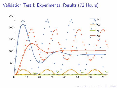
Validation Test I: Experimental Results (72 Hours)

Possible Source of Oscillations

Discretization-induced (discrete time, discrete state)

Delay-induced (discrete delay); Hopf bifurcation

New “Large Workflow” Assumptions

Provision resources based on individual submissions

N = jobs per user submission � M = max instances

User-specified workflow “deadline”

Tdeadline � τRT > τRI > ∆t

User-specified estimate of average job lifetime, τRI .

Meet deadline or run out of money; minimize waste and cost

Acknowledgments

Todd Miller @ UW - MadisonCenter for High Throughput Computing, HTCondor

Frank Wurthwein @ UCSDOpen Science Grid, Executive Director

Jeffery Dost @ UCSDOpen Science Grid, Glidein Factory Operations

Edgar Fajardo @ UCSDOpen Science Grid, Software

Questions?