Working paper

Free Provision and Demand for Health Products

Evidence from follow-up of a randomised control trial study in Bangladesh

Minhaj Mahmud Ananta Z. Neelim Abu Mohd Naser Titu

December 2014

When citing this paper, please use the title and the following reference number: S-31109-BGD-1

1

PROJECT REPORT

PROJECT NUMBER 1-VCS-VBAN-V3025-31109 Bangladesh Growth Research Program

International Growth Centre

Free Provision and Demand for Health Products: Evidence from follow-up of a randomised control trial study in Bangladesh

By

Minhaj Mahmud Ananta Z. Neelim

Abu Mohd Naser Titu

December 2014

2

Free Provision and Demand for Health Products: Evidence from follow-up of a randomised control trial study in Bangladesh

By

Minhaj Mahmud1

Ananta Z. Neelim2

Abu Mohd Naser Titu3

Abstract We elicit demand for a water disinfectant tablet (Aquatab) among rural households in

Bangladesh in the specific case of free provision. We did not find any significant effect of

free provision on long-run demand. In fact, even a year later of the efficacy study, both the

free users of Aquatab and non-users were willing to pay roughly 50 percent of the announced

market price suggesting that free provision did not dampen long run demand. Our results also

suggest that there is a strong effect of arbitrary price anchors on individuals’ willingness to

pay, irrespective of free provision. However, suggestive of “coherence”, we find more people

are willing to purchase at higher discounts (lower price).

Keywords: health product, willingness to pay, anchoring

JEL Codes:

Acknowledgements: This study leverages on an existing randomised control trial study on health impact of the water disinfectant tablet as well as water storage vessel conducted by the Water Sanitation and Hygiene Research Group of the International Centre for Diarrhoeal Disease Research, Bangladesh (icddr’b) during 2011-2012. We gratefully acknowledge the support of Leanne Unicomb and her research group for allowing us to conduct this follow-up study. We also express our gratitude to International Growth Centre (IGC) for funding of this study. The usual disclaimer applies 1 BRAC University, Bangladesh. Corresponding author. Email: minhajmahmud@gmail.com 2University of Nottingham, Malaysia 3Emory University, USA

3

1. Introduction

Understanding individual demand for health products is important for various stakeholders

involved in water demand management as well as for policy makers in developing countries.

There is an existing policy debate on whether health products in developing countries should

be provided at zero prices (Sachs, 2005), or on a cost-sharing basis between the state and

consumers (Easterly 2006). The main argument against free provision is that it is financially

unsustainable and more importantly it generates wastage by providing wrong incentives. Cost

sharing advocates argue that allowing consumers to bear some cost of the good incentivises

its proper usage and more importantly, screens out people who do not have any valuation for

the product. While free provision advocates suggest that policy goal, especially with regards

to products which prevent communicable diseases, should be to ensure that the maximum

share of the population is included and that asking individuals to share the cost can

sometimes become prohibitively expensive for the neediest. One key element that has been

missing from the debate is that, whether the estimation of demand is contaminated by free

provision of goods via the formation of a sense of entitlement from previous free provision.

This study builds on a recently implemented randomised control trial study where point-of-

use (portable) water treatment products were provided free amongst a study population. We

aim to investigate whether positive prices; and subsequently zero prices, act as arbitrary

anchors, affecting users’ willingness to pay for the same health product.

Some very interesting findings have emerged recently from research on some core

issues surrounding the above policy debate. Firstly, there is evidence that asking individuals

to share costs has huge implications on uptake. Cohen and Dupas (2010) based on a

randomized controlled trial(RCT) experiment conclude that cost-sharing does indeed

decrease demand for insecticide treated bed-nets (ITNs) by sixty percent when subsidies are

4

reduced from 100 to 90 percent. Similarly in Kenya, when schools were asked to pay

between 20 to 60 percent of the market price, as opposed to free provision, uptake dropped by

56 percentage points (Kremer et al 2011). A survey article by Bates et al (2012) also

documents other instances of substantial drops in uptake of health products when consumers

were asked to share costs vis a vis free provision. Secondly, there is evidence that free

provision does not lead to underutilisation of health products. Dupas (2014a) in a survey

article provide evidence from RCT experiments that high subsidies (including free provision)

do not significantly alter usage of insecticide treated bed nets or chlorine dispensers.

Furthermore there is also no evidence that highly subsidized or freely provided products are

valued at a lower level than unsubsidized products. For example, Dupas (2009) and Cohen

and Dupas (2010) show that there is no statistical difference between the usage rates of bed

nets amongst individuals who received it for different prices. Relatedly, Ashraf et al (2010)

show that paying more for a water treatment product does not lead to higher usage rate due to

sunk cost effects1. There is also evidence that the intensity in the drop in demand is larger

when price increase from zero (free provision) to a small positive price compared to drops in

demand due to further increases in price (Kremer et al, 2011). This is perhaps driven by the

fact that the expectation of even small cost sharing on the part of the neediest people (the

poor) can be enormous and as a result they will be screened out. In fact, Tarozzi et al (2013)

show that alleviating financial constraints through micro-loans can significantly increase

demand for bed nets even when individuals are asked to pay the full price for the product.

However, they also show that demand with micro-loans is still a half of that when bed nets

are provided for free. This suggests that financial constraints cannot fully explain drops in

demand due to financial constraints.

1 Sunk cost effect arises from the idea that people who pay for a particular product derive displeasure for not

utilizing something that they have paid for (Thaler, 1980).

5

Another possible explanation for the drop in demand is with regards to reference dependence

or entitlement formation i.e. households that receive products for free or at a subsidized rate

(during a necessary promotion phase to facilitate learning of experience goods) might anchor

their valuation of the product to the free or subsidized rate and subsequently reduce demand

when asked to pay a higher price (Koszegi and Rabin, 2006). Under such reference dependent

preferences it might be the case that short run free provision may reduce long run uptake

(Dupas, 2014b) if the effect of entitlement formation is greater than the effect of positive

experience of using the product. In fact in Guatemala, there is strong evidence even after

observing high efficacy (39 percent less diarrhoea) households who received flocculants –

disinfectants for free were not more likely to demand when they were to purchase at a

positive price (Luby et al. 2008). Furthermore, Luoto et al. (2012) in a RCT study conducted

in Bangladesh, show that households that received water treatment products (chemical

products) for free later exhibited lower willingness to pay than the control group. However,

there is also evidence of increases in long-run demand following short run subsidy. For

example, Dupas (2014b) shows that short run subsidies lead to higher adoption for bed nets in

Kenya through positive learning effects which dominates anchoring or entitlement effects. In

fact reduced form estimates show no evidence of anchoring effects influencing households’

uptake of bed nets.

In this paper we elicit demand for a water disinfectant tablet among rural households

in Bangladesh. Our study leverages on an existing RCT study analysing the health impact

(efficacy) of the water disinfectant tablet as well as water storage vessel whereby treatment

households received one or more product free of costs for ten months versus control

households receiving none of these. Using Becker-DeGroot-Marschak (Becker et al 1964),

auction procedure we elicit willingness to pay (WTP) and investigate whether zero prices and

subsequently positive prices act as arbitrary anchors affecting users’ WTP for heath product.

6

Our design allows us to identify the effect of entitlement as well learning in the special case

of free provision. Unlike Dupas (2014b), we experimentally vary price anchors for people

who had previously received the product for free in the efficacy study versus people who had

not received the product, and examine the effects of these price anchors on demand.

We did not find any significant effect of free provision on long-run demand. In fact,

even a year later of the efficacy study, both the free users of Aquatab and non-users were

willing to pay roughly 50 percent of the announced market price suggesting that free

provision did not dampen long run demand. This is consistent with the findings of Dupas

(2014b) who found that long run uptake of preventive health product (bed nets) was not

affected by past prices. Our results also suggest that there is a strong effect of arbitrary price

anchors on individuals’ willingness to pay, irrespective of free provision. However,

suggestive of “coherence”, we find more people are willing to purchase at higher discounts

(lower price). This “coherent arbitrariness” preference is consistent with earlier laboratory

findings of Ariely et al. (2003), which suggest that ‘people respond sensibly to noticeable

changes in price although their responses base initially around a normative anchor’(here

announced market price). To our knowledge this is the first experimental evidence from a

developing country demonstrating such “coherent arbitrariness” in individual’s preference for

a health product. Our paper also contributes to the emerging literature on pricing of health

products as well as on the policy debate of free provision versus cost sharing.

The remainder of the paper is organised as follows. Section 2 documents the

background study setting. Section 3 discusses the conceptual framework, experimental design

and study protocol. Section 4 discusses the results of our experiment and Section 5 concludes

the paper.

7

1. Background: Efficacy Study

The present study leverages on a RCT study that looks into the impact of chlorination and

safe storage of tube-well water on childhood diarrhoea in rural Bangladesh. This efficacy

study was carried out by the icddr,b across 87 randomly selected villages in Fulbaria

subdistrict of Mymensingh district of Bangladesh. In these 87 villages, 1800 households were

randomly selected based on the eligibility criteria of having one household member between

the ages of 6 months to 18 months. These 1800 households were further randomly sampled

into three groups and were assigned to three study arms defined as Control, Storage and

Aquatab. Households assigned to the control arm did not receive any products, whereas

households assigned to the Storage and Aquatab arms both received a safe storage vessel. In

addition only households in the Aquatab arm were given free (point of use) water treatment

tablets. Across any given study village, participants from all three study arms were present.

These study households were visited for ten unannounced follow ups to ascertain the usage of

these products (safe storage vessel and Aquatab) and subsequent impacts of these on

childhood diarrhoea. The results of the intervention suggest that there was very high levels of

uptake and usage of products. Over eighty-five percent of the subjects utilised their safe

storage in both the Aquatab and Safe Storage arm across ten follow ups. Amongst the people

who used the safe storage vessel in the Aquatab arm, 83 percent of them had chlorine residue

in the stored water, suggesting high usage rates of Aquatab in that particular study arm. In

terms of impact on childhood diarrhoea, safe storage vessel (with or without the usage of

Aquatab) drastically reduced diarrhoea prevalence. The prevalence rate of diarrhoea was 64

(69) percent of that of the control arm in the Aquatab (Safe Storage) arm. However, there was

no statistically significant difference in the prevalence rate of diarrhoea across the Aquatab

and Self-Storage arm. (Naser, 2013)2. At the end of the efficacy study each household in the

2 http://www.icddrb.org/publications/doc_download/7892-vol-11-no-4-english-2013

8

control arm were given a free safe storage vessel. We re-visited these households (n= 500)3

twenty months after the completion of the efficacy trial to examine household willingness to

pay for Aquatabs4.

2. Conceptual Framework and Experimental Design

The main experimental intervention of the experiment follows from the behavioural evidence

that individuals’ preferences are malleable and that it can be dependent on external

environments (Ariely et al 2003). Specifically, it has been shown that individuals willingness

to pay for a particular product can be altered by informing them about a single price of that

particular product (past or present), price of a close substitute, an unrelated product and even

an arbitrarily generated price(see for example; Adaval and Monroe, 2002; Adaval and Wyer,

2011; Chapman and Johnson, 2002; Krishna, Wagner, Yoon, and Adaval, 2006; Nunes and

Boatwright, 2004; Simonson & Drolet, 2004; Tversky and Kahneman, 1974). The

information about prices has been shown to act as anchors when individuals express their

willingness to pay for the product in question. In the context of Aquatab, household

willingness to pay can be dependent on learning effect (due to usage of this product) or

reference dependence (potential entitlement formation due to free provision)5.

. 3 There was attrition due to multiple factors during the first RCT, which lasted about 11 months. In addition

further attrition took place between our study and the first RCT. 4 Although our initial plan was to conduct this experiment six months after the completion of the RCT study, we

were unable to do so due to research grant approval and other administrative delays. 5 The Aquatab recipient households are the only ones in the sample who may have reference dependent

valuation of the product due to free provision. If they were to be asked to value it they may express a lower

willingness to pay for these water disinfectants than the non-recipient households. However, at the same time,

these households were also the only ones who would observe the health benefits associated with using these

tablets (i.e. positive learning effect). While the health benefits from using (usage rate of 85%) the only tablets

were negligible one cannot discount the possibility that the households which received Aquatabs attributed the

improvements in health to Aquatabs and not to the safe storage vessels. If that is indeed the case then that would

provide a positive experience for these households leading them to have a higher valuation for Aquatabs. This

9

Use of two separate price anchor in our experiment allows us to disentangle these two effects.

Prior to the willingness to pay elicitation task, half of the participants, across three arms of

the efficacy study (i.e. Control, Aquatabs, Storage) are informed that the expected market

price for two weeks supply of the product will be Tk 20 (High price treatment; hereinafter

HIGH) and the other half were told that this was Tk 10 (Low price treatment; hereinafter

LOW)6. For the households that did not receive Aquatabs for free (control and storage arm in

the efficacy study), these prices would act as the only price anchors. If indeed preferences

were dependent on initial price anchors, valuation of Aquatabs would be significantly higher

for households in the HIGH compared to households in the LOW.

On the other hand for households that received Aquatabs for free during the efficacy

study, valuation of Aquatabs would be dependent on two anchors: the price anchor that we

introduced in the experiment and the anchor from receiving Aquatabs for free during the

efficacy study. The difference in valuation of Aquatabs across the two price treatments

(HIGH vs LOW) thus would be the effect of price anchor conditional on free provision. If the

estimate of the expected market price follows a simple linear combination of the two anchors

for these households, 𝒙 (𝒂𝒏𝒄𝒉𝒐𝒓 𝟏) + 𝒚 (𝒂𝒏𝒄𝒉𝒐𝒓 𝟐), 𝒘𝒉𝒆𝒓𝒆 𝒙 + 𝒚 ≤ 𝟏}, then it will be

significantly different for these households compared to the ones who only receive one

anchor. If that is the case then the valuation of the product will be different across households

that did or did not receive Aquatabs for free. Specifically the effect of price anchors (HIGH

and LOW) would be smaller in the case where it is conditioned on free provision versus the

case when it is not.

poses a significant problem in examining the effect of free provision on willingness to pay as now it is entangled

with the effects of positive experience of using the products. 6 Aquatab is not readily available in the markets in Bangladesh. The cost of Aquatab in the USA is about Taka

11-12 per two weeks supply during the period of study. However, considering commercial costs of importing

and logistics, the actual fully market price for two weeks supply could indeed be around Tk 20. This means that

the price anchor we chose for our study represented either full price (Taka 20) or fifty percent subsidy (Tk 10).

10

3.1 Willingness to Pay Elicitation: Becker-DeGroot-Marschak (BDM) auction

To elicit demand (willingness to pay) for Aquatab we used a modified version of the Becker-

DeGroot-Marschak (BDM) auction procedure (reference). In the standard BDM auction,

where bidders’ weakly dominant strategy is to reveal their true valuation, a bidder first

submits her bid for the good in question. Experimenter then draws a random number from a

pre-specified distribution or from a range of price which is informed to the bidder. If the

submitted bid is greater than the random price, the bidder wins and purchases a pre-specified

unit of the good at the randomly drawn rice. That is subjects are usually informed a price

range from which the actual transaction price of that particular product, for which the

willingness to pay is being elicited, lies. Subsequently, they are asked to state their WTP for

that product. Once the task is completed, the experimenter draws a random number from that

range. Conditional on the bid and the number drawn the responder gets the opportunity to buy

the product. If the bid is greater than or equal to the randomly drawn number then the

respondent qualifies (wins) to purchase the product, otherwise she doesn’t. BDM procedure

elicits incentive compatible responses given that the respondents understand the procedure.

Sometimes it might be cognitively difficult on the part of respondents. To facilitate better

understanding, we use a modified BDM procedure whereby subjects are asked a string of

multiple binary choice questions to respond in order to express their valuation for the

product. The way we define the BDM procedure is slightly different and instead of reporting

just one value for WTP, we ask each respondent if they were willing to pay at various

discounted prices. The subjects were asked about their willingness to pay about various prices

one by one.

Specifically, our study participants were told that that the discount they will get in the survey

will range from 10 percent to 80 percent (90 percent in the HIGH price treatment). They were

informed that the actual discount rate was predetermined by a lottery and was kept inside an

11

envelope and was even unknown to the survey administrator. Furthermore they were notified

that both the administrator and the participant would open the envelope after the participants

have answered a set of questions about their willingness to buy the product at different prices.

The rule for winning the auction and hence eligibility to buy the product was as follows:

based on the answers given and the discounted price in the envelope, if the participant

indicated that s/he would be willing to purchase the product at that (envelop) price, and then

s/he would get the opportunity to do so. However, if she indicated that she would not be

willing to purchase the product at that discounted price then she would not get the

opportunity to purchase it. This rule was reiterated and a full practice round of this process

was conducted to ensure that participants clearly understand the procedure/protocol and

hence the implication of their responses.

Assignment of participants to HIGH or LOW treatment was done randomly. All the

participating households were ordered in ascending way based on the study ID from the

efficacy study after which a random number generator was utilised to assign each of these

participating households a number between 0 and 1. If the number assigned to IDs was

greater than 0.5 they were assigned to HIGH and if the number assigned to IDs was less or

equal to 0.5 they were assigned to LOW treatment group.

3.2 Experimental Protocol

All protocols across HIGH and LOW treatments were the same, whereby they were

informed about the purpose of the day’s visit, given a small account(information) on the

health benefits of using Aquatab, informed about the promotional price opportunity and the

lottery process and then asked to fill out a small questionnaire at the end. They were informed

about the purpose of our research, which was to understand the demand for Aquatab.

Each available household from the efficacy study were revisited and an adult member

who is responsible for making household decisions was approached for an interview to elicit

12

demand for Aquatab. For the benefit of the study population, we provided a small recap about

the health benefits of water disinfectant Aquatab and then informed them of the expected

market price for two weeks supply. We notified them that as a survey participant there will be

an opportunity to purchase two weeks supply of Aquatab at a discounted price determined by

a pre-determined lottery (the willingness to pay elicitation task). The participants were given

descriptions of the lottery process and were then asked whether they would participate in it. It

was made clear to them that if they become eligible to buy the product through winning the

auction they will be obliged to buy two weeks supply of Aquatab at the lottery determined

discounted price. Upon completion of the WTP elicitation task each subject was interviewed

using a set questionnaire to get information on household characteristics and health

behaviour.

4. Results

Our study was conducted among 1500 households that we could finally identify and revisit

out of the initial 1645 households that were surveyed in the original RCT efficacy study. This

translates to a 91.2 percent revisit rate after 20 months of completion of the last follow up of

the efficacy trial. Out of these 1500 households, 488 (32.5 percent), 499 (33.27 percent) and

513 (34.2 percent) were in the Aquatab, Safe Storage and Control treatments in the original

study. In our case, 753 households (49.5 percent) are in the HIGH treatment and the rest, 757

households are in the LOW treatment. As a result of randomization, of the households

assigned in the HIGH treatment, 32.8%, 33.4% and 33.8% belong to the Aquatab, Safe

Storage and Control treatments respectively of the original study. In the LOW treatment,

these numbers were roughly similar, 32.2, 33.2 and 34.6 percent respectively (see Appendix

1).

The baseline sample characteristics are reported in Table 1. The average household

size was 5.35 members and 96 percent of these households owned their homestead land. The

13

average total expenditure per month was around Tk 7950, while the mean years of schooling

for the mother of the children was 4.7 years. The fathers on average had lower levels of

education with a mean of 3.44 years. The average landholding per household was 52.45

decimals of land and around 40 percent of the households had access to microfinance loans.

Four percent of the households had female heads and 2.5 percent of the households had a

disabled member. In terms of prevalence of diseases, 9 percent of the households reported

that a child in their household has experienced diarrhoea in the last two days, while 19.2

percent reported that the same for fever.

Randomization and Balance Check

To check balance across our treatments we conduct two randomization checks with

regards to observable characteristics collected during the baseline of the efficacy study as

well as during our willingness to pay study. Specifically, we conduct balance checks (i)

across our HIGH and LOW treatments and (ii) across HIGH and LOW treatments within

each original study arms. These are presented in Table 1 and Table 2 respectively. According

to Table 1, in all of the observable characteristics, there is no statistical difference across the

HIGH and LOW treatments. With regards to individual study arms as well, generally there is

evidence of balance across the subgroups. In the Aquatab and the Storage arms none of the

observable characteristics is different across the HIGH and LOW treatments at a significance

level of 5 percent. However, in the Control arm access to microfinance is 10.7 percentage

points larger in the HIGH treatment compared to that in the LOW treatment (p-value =0.01;

T-test). While we do not envision this difference to significantly affect the WTP estimates

due to the relatively low prices of Aquatab, we control for it in our regression analysis.

Experimental Results

We begin by analysing the individual decision to participate in the willingness to pay

elicitation study (BDM Auction). Each respondent, after they were demonstrated the BDM

14

lottery process was asked whether they would like to participate and buy the product. Overall

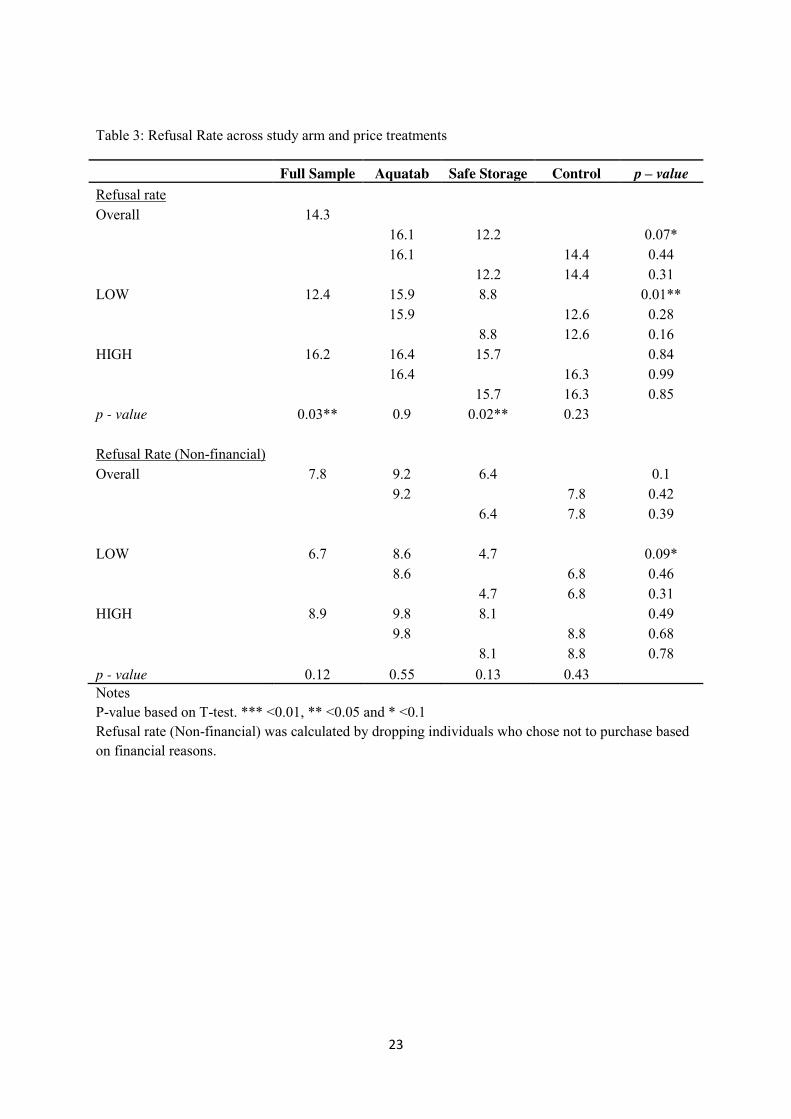
a significant portion, 14.3 percent, of the participants chose not to participate (see Table 3).

The main reasons for not choosing to participate in this process were related to either

disinterest in the product or financial constraints (see Table 4). Out of the participants who

chose not to buy Aquatab, 57 percent of the respondents cited disinterest in the product, 45

percent cited financial constraints and 21 percent cited preference of other methods of water

purification as reasons for their decision not to purchase Aquatab7. Across study arms refusal

rate to not purchase Aquatab was highest in the Aquatab arm, which was 16.1 percent. This

refusal rate was 12.2 percent and 14.4 percent in the Safe Storage and Control arm

respectively. The difference between refusal rates is not statistically different (at p - value

<0.05, pair wise t-tests) between any of the study arms. Conversely, we find statistically

significant difference across the price treatments for the whole sample (p – value = 0.04; T-

Test): In the HIGH treatment, 16.2 percent of the participants refused to participate which

was larger than that in the LOW treatment, 12.4 percent. However this difference across

HIGH and LOW treatment is not consistent across the study arms and is driven by behaviour

in the Safe Storage arm. This difference is 0.4 percentage points in the Aquatab arm (p –

value = 0.90; T-test), 7 percentage points in the Safe Storage arm (p – value = 0.02, T-test)

and 3.7 percentage points in the Control Arm (p – value = 0.23). Furthermore, if we use the

subset of the people who identified that financial constraint was not the reason for their

refusal to buy the product, the difference in refusal rates across HIGH and LOW treatment

becomes statistically insignificant for the whole sample and across all the study arms (Table

3). This suggests that price does not act as a signal of quality when individuals decide

whether to choose or not choose to purchase the product with this effect being smallest for

the participants in the Aquatab arm, who have the most experience in using the product. In

7 This was a multiple answers question.

15

terms of valuation of the product (conditional on not refusing to purchase the product),

participant willingness to pay was relatively large. In the LOW treatment 33.4 percent of the

participants wanted to buy the product at Tk 9, which represented a mere ten percent

discount. Similarly, around 65 percent of the participants were willing to purchase the

product at least 50 percent discount, i.e. Tk 5. From Figure 1 and Table 4, we can observe

that the mode willingness to pay was Tk 9 followed by Tk 5. This suggests that a significant

portion of the participants were willing to share a big fraction of the full expected market

price and majority of the participants were willing buy Aquatab at a 50 percent discounted

price in the LOW treatment. At 80 percent discount, which is Tk 2, almost all the

participants, were interested in buying the product. In the HIGH treatment we see similar

patterns in bidding behaviour. 16.1 percent of the participants wanted to buy Aquatab at the

10 percent discounted price of Tk 18. The mode willingness to pay in the HIGH treatment

was Tk 10 (50 percent discount) followed by Tk 18 (90 percent discount). At the 50 percent

discounted price, 47 percent of the participants were willing to purchase Aquatab, which

went up to 99 percent when discount was 90 percent, i.e. Tk 2. In both these treatments it is

important to notice that below the 50 percent discount, where individuals are expected to pay

more than half of the announced price, there is a huge drop in demand. This along with the

observation significant maximum bids at 50 percent discount value suggests that there is

some systematic heuristics that people utilise when participating in these willingness to pay

elicitation tasks.

Based on the bidding responses we create a demand schedule which is represented in

Figure 3. From the Figure 3, we can see that quantity demanded, measured as the proportion

of respondents willing to buy the product at any particular price, is negatively related to these

particular bid(prices). This is true for in both HIGH and LOW treatments. This shows that

preferences for Aquatabs translate to normal demand for the product. At the same time the

16

figure also exhibits the effect of arbitrary price anchors. The demand exhibited by individuals

in the HIGH treatment is systematically higher than that in the LOW treatment In terms of

both mean (Table 6, p-value: <0.01, T-test) and distribution (Figure 1, p-value: <0.01,

Kolmogorov Smirnoff) WTP in the LOW and HIGH treatments are statistically different.

While we find huge impacts of the price treatments on WTP, we find very little

difference across the three study arms within each of these treatments. From Figure 2, Figure

4 and Figure 5 we can observe that there is very little difference in the WTP elicitation across

study arms. In fact from Table 5 (right-most column), we can see that none of mean WTP

across the study arms (within each price treatment) are statically significant. Furthermore, the

distributions of WTP are also not statistically significantly different (Figure 2).

To test the effect of free provision on future demand, in Section 3, we argued that if

free provision does affect willingness to pay then the impact of our arbitrary price anchors

will be smaller in the Aquatab arm compared to the Control arm. To test whether that is the

case, we run set of regressions. Some of these regressions control for household level

characteristics and village level heterogeneity and thus also provide a validation check for all

the results presented in this section so far. The regression estimates are reported in Table 7.

We utilise the maximum WTP elicited by households as the main dependent variable in all

our different specification. In the first three columns, we analyse the unconditional impact of

price anchor treatment on maximum WTP. Column (1) reports results from the specification

which does not account for either household level or village level heterogeneity. Column (2)

and (3) report estimates accounting for those progressively. In all three columns LOW

treatment is the default omitted category. From Table 7, we see that coefficient for HIGH

treatment is positive and significant suggesting that the effect of price anchors is robust to

household and village level heterogeneity. In addition we find that households that have

larger land holding have a higher willingness to pay for Aquatab. If we consider landholding

17

as a proxy of wealth, this result is perhaps not surprising. All other household characteristics

do not influence the demand for Aquatab, including that of Microfinance access.

In columns (4) through to (6) we report effect of price treatment conditional on study

arms. The main difference across these specifications is the same as in columns (1) - (3) in

terms of accounting for household and village level heterogeneity. In these estimates LOW

treatment Aquatab arm acted as the default omitted category. Based on the coefficient

estimates from the regressions (panel A) we report the difference estimates of price treatment

across the three study arms in panel B. From these estimates, not surprisingly, we can observe

that there is a strong significant effect of price treatments in all three of the study arms. More

importantly, we can also observe that the strength of the price treatment effect is not very

different between the three arms. As observed the LOW –HIGH difference between the

Aquatab and control arm ( −𝚫𝑪) which is the difference in the strength of the price treatment

effect between Aquatab and control arm, is not significantly different from zero. This

suggests that in our sample we find no evidence of effect of free provision on long term

demand for Aquatab.

3. Conclusions

In this paper we elicit long-run demand for water disinfectant tablets in rural areas in

Bangladesh in the specific case of free provision. We leverage on an efficacy trial, completed

twenty months prior to this study, which provided a group of people the opportunity to use

the product for free for ten successive months. Using this variation and by introducing price

treatments (HIGH and LOW), we investigated whether free provision (i.e. zero prices) and

positive prices act as arbitrary anchors in user’s willingness to pay.

Our results provide evidence that free provision did not dampen long run demand for

the water disinfectant: 20 months later free majority users were willing to pay roughly 50%

of the announced market price for Aquatabs with no difference across people who

18

experienced free provision or not. While we do not find long run effects of free provision

through entitlement formation, we cannot discount the possibility that if we investigated short

run impacts the results would have been different as free provision would have been more

salient in that case. However, our results are consistent with findings of Dupas (2014 b), who

also show that short run subsidies have low impacts on long run demand.

We find that both the mean and distribution of WTP is significantly higher in high

price treatment group (HIGH) compared to low price treatment group (LOW), irrespective of

free provision (experience). This is quite interesting and suggestive of powerful effect of

anchoring: announced market price acts as powerful anchor resulting in higher valuation for

the product. While our results show a strong effect of arbitrary price anchors on individuals’

willingness to pay, interestingly we also find willingness to pay was systematically related to

price discounts: at higher discount prices, the share of people willing to pay for two weeks

supply of Aquatab increased. According to Ariely et al (2003), this behavioural pattern is

suggestive of “coherent arbitrariness” whereas people respond sensibly to noticeable changes

in price, but their responses are based around initial normative anchor (in our case the

announced market price acted as arbitrary anchor). As suggested by Ariely et al ( 2003) , the

implication of “coherent arbitrariness” is that if price changes are not drawn to the attention

of the users, i.e. full information of changes in prices (or quality) are not provided, they may

not respond reasonably reflecting fundamental values. Dupas (2014b) also points out that

estimating the effect of subsidies (full or partial) by providing full information about non-

subsidized price is of direct policy interest and that for products which are not familiar or

whose price is relatively unknown such as water disinfectant in our case anchoring effect

might be larger.

Knowing individuals’ demand for health products such as water disinfectant

technology is important to stakeholders involved in water demand management as well as for

19

policy makers in developing countries. We did not find evidence of users’ long-run demand

being affected by initial subsidies and our findings suggest that people are willing to share

costs up to a level (on average majority of participants regardless of past experience, were

willing to pay at least 50% of the announced market price) when given full information about

the potential retail price of the product. We believe future demand assessment exercises

would benefit from the findings of our study as it explicitly addresses the issue of anchoring

in willingness to pay elicitation.

Reference

Adaval, R., & Wyer Jr, R. S. (2011). Conscious and nonconscious comparisons with price

anchors: Effects on willingness to pay for related and unrelated products. Journal of

Marketing Research, 48(2), 355-365.

Adaval, R., & Monroe, K. B. (2002). Automatic construction and use of contextual

information for product and price evaluations. Journal of Consumer Research, 28(4),

572-588.

Ariely, D., Loewenstein, G., & Prelec, D. (2003). "Coherent Arbitrariness": Stable Demand

Curves Without Stable Preferences. The Quarterly Journal of Economics, 118(1), 73-

105

Ashraf, N., Berry, J., & Shapiro, J. M. (2010). Can Higher Prices Stimulate Product Use?

Evidence from a Field Experiment in Zambia. American Economic Review, 100(5),

2383-2413.

Bates, M. A., Glennerster, R., Gumede, K., & Duflo, E. (2012). The Price is Wrong. Field

Actions Science Reports. The Journal of Field Actions, (Special Issue 4).

Becker, Gordon M., Morris H. DeGroot, and Jacob Marschak. "Measuring utility by a

single‐response sequential method." Behavioral Science 9, no. 3 (1964): 226-232.

Chapman, G. B., & Johnson, E. J. (2002). Incorporating the irrelevant: Anchors in judgments

of belief and value. Heuristics and biases: The psychology of intuitive judgment, 120-

138.

Cohen, J. and Dupas, P. (2010) Free Distribution or Cost-Sharing? Evidence from a

Randomized Malaria Prevention Experiment. Quarterly Journal of Economics 125(1)

1-45.

20

Dupas, P. (2009). What matters (and what does not) in households' decision to invest in

malaria prevention? The American Economic Review, 224-230.

Dupas, P. (2014a). Getting essential health products to their end users: Subsidize, but how

much? Science, 345(6202), 1279-1281.

Dupas, P. (2014b). Short‐Run Subsidies and Long‐Run Adoption of New Health Products:

Evidence From a Field Experiment. Econometrica, 82(1), 197-228.

Easterly, W., & Easterly, W. R. (2006). The white man's burden: why the West's efforts to aid

the rest have done so much ill and so little good. Penguin.

Kremer, M., Miguel, E., Mullainathan, S., Null, C., & Zwane, A. P. (2011). Social

engineering: Evidence from a suite of take-up experiments in Kenya. Working Paper.

Kőszegi, B., & Rabin, M. (2006). A model of reference-dependent preferences. The

Quarterly Journal of Economics, 1133-1165.

Krishna, A., Wagner, M., Yoon, C., & Adaval, R. (2006). Effects of extreme-priced products

on consumer reservation prices. Journal of Consumer Psychology, 16(2), 176-190.

Luby, S. P., Mendoza, C., Keswick, B. H., Chiller, T. M., & Hoekstra, R. M. (2008).

Difficulties in bringing point-of-use water treatment to scale in rural Guatemala. The

American journal of tropical medicine and hygiene, 78(3), 382-387.

Luoto, J., Mahmud, M., Albert, J., Luby, S., Najnin, N., Unicomb, L., & Levine, D. I. (2012).

Learning to dislike safe water products: results from a randomized controlled trial of

the effects of direct and peer experience on willingness to pay. Environmental science

& technology, 46(11), 6244-6251.

Naser, A. (2013) Randomized controlled trial evaluating health impact of treating and safely

storing shallow tubewell drinking water in rural Bangladesh. Health Science Bulletin

11(4), 1-8.

Nunes, J. C., & Boatwright, P. (2004). Incidental prices and their effect on willingness to pay.

Journal of Marketing Research, 41(4), 457-466.

Sachs, J. (2005). The end of poverty: How we can make it happen in our lifetime. Penguin

UK.

Simonson, I., & Drolet, A. (2004). Anchoring effects on consumers’ Willingness‐to‐Pay and

Willingness‐to‐Accept. Journal of consumer research, 31(3), 681-690.

Tarozzi, A., Mahajan, A., Blackburn, B., Kopf, D., Krishnan, L., & Yoong, J. (2013).

Micro‐Loans, Bednets and Malaria: Evidence from a Randomized Controlled Trial.

American Economic Review, 1.

21

Tversky, A., & Kahneman, D. (1974). Judgment under uncertainty: Heuristics and biases.

Science, 185(4157), 1124-1131.]

Table 1: Baseline sample characteristics

Variable Full

Sample Treatment High Price

Treatment Low price

P value of difference

Average Total Expenditure+ 7942 8075 7812 0.27

Access to Microfinance Loans+ 0.4 0.41 0.39 0.51

Diarrhoea of < 5 child in the last 2 days+ 0.09 0.091 0.086 0.84

Fever of <5 child in the last 2 days+ 0.192 0.2 0.18 0.30

Land Holding (Non Homestead) 52.45 48.77 56.07 0.30

Education of Mother 4.63 4.53 4.71 0.35

Education of Father 3.68 3.56 3.8 0.27

Household Size 5.35 5.32 5.37 0.65

Female Household Head 0.04 0.04 0.04 0.84

Disabled Member in Household 0.025 0.03 0.02 0.47

Notes: P-values based on T-test. *** <0.01, ** <0.05 and * <0.1 + These values were collected as a part of this round of data collection. All the other variables were collected during the baseline of the efficacy study.

22

Table 2: Baseline Sample Characteristics across study arms and price treatments

Notes P-value based on T-test. *** <0.01, ** <0.05 and * <0.1 + These values were collected as a part of this round of data collection. All the other variables were collected during the baseline of the efficacy study.

Variable Aquatab Storage Control

High Low p value High Low p value High Low p value

Average Total Expenditure+ 8236 7784 0.24 7897 7822 0.83 8046 7829 0.64

Access to Microfinance Loans+ 38.1 38.9 0.85 37.9 43.0 0.24 45.8 35.1 0.01**

Diarrhoea of < 5 child in the last 2 days+ 0.06 0.06 1.00 0.09 0.10 0.42 0.118 0.107 0.70

Fever of <5 child in the last 2 days+ 0.17 0.18 0.64 0.15 0.21 0.09* 0.229 0.219 0.79

Land Holding (Non Homestead) 44.1 51.5 0.54 47.1 50.8 0.72 54.9 65.4 0.45

Education of Mother 4.7 4.6 0.77 4.5 4.76 0.52 4.35 4.76 0.21

Education of Father 3.44 3.8 0.35 3.6 3.9 0.40 3.62 3.67 0.90

Household Size 5.29 5.47 0.33 5.27 5.4 0.51 5.41 5.26 0.41

Female Household Head 0.05 0.05 1.00 0.04 0.02 0.21 0.04 0.05 0.47

Disabled Member in Household 0.03 0.03 1.00 0.02 0.02 0.77 0.03 0.11 0.11

23

Table 3: Refusal Rate across study arm and price treatments

Full Sample Aquatab Safe Storage Control p – value Refusal rate

Overall 14.3

16.1 12.2

0.07*

16.1

14.4 0.44

12.2 14.4 0.31

LOW 12.4 15.9 8.8

0.01**

15.9

12.6 0.28

8.8 12.6 0.16

HIGH 16.2 16.4 15.7

0.84

16.4

16.3 0.99

15.7 16.3 0.85

p - value 0.03** 0.9 0.02** 0.23

Refusal Rate (Non-financial) Overall 7.8 9.2 6.4

0.1

9.2

7.8 0.42

6.4 7.8 0.39

LOW 6.7 8.6 4.7

0.09*

8.6

6.8 0.46

4.7 6.8 0.31

HIGH 8.9 9.8 8.1

0.49

9.8

8.8 0.68

8.1 8.8 0.78

p - value 0.12 0.55 0.13 0.43 Notes P-value based on T-test. *** <0.01, ** <0.05 and * <0.1 Refusal rate (Non-financial) was calculated by dropping individuals who chose not to purchase based on financial reasons.

24

Table 4: Reasons for not buying

Reasons for not buying %

Not interested in the product 57.0 Product will not work 8.4 Purify water in other way 21.0 Will not pay for water purification 17.8 Do not trust calculations 4.2 Taste of water deteriorates 5.1 Other people said product doesn’t work 1.9 Do not have money 45.3 Have to discuss with other members of the Household 9.3 Do not believe in lotteries 6.5

Notes: Question had provisions for multiple answers.

25

Table 5: Distribution of Maximum Willingness to Pay

Max WTP

Full Sample AQUATAB STORAGE CONTROL High Low High Low High Low High Low

< 2 1.0 0.5 0.5 0.0 1.4 0.9 0.9 0.4

2 1.1 2.0 1.5 1.0 1.4 2.2 0.5 2.6

3 0.3 2.4 0.5 1.0 0.5 3.0 0.0 3.0

4 1.8 5.1 1.0 3.9 1.4 4.8 2.8 6.5

5 7.5 25.4 8.3 28.8 5.7 26.0 8.5 21.7

6 2.1 12.5 1.5 16.6 2.4 9.5 2.4 11.7

7 2.7 11.0 1.5 10.7 2.4 11.3 4.2 10.9

8 4.5 7.7 2.4 7.3 4.8 6.9 6.1 8.7

9 3.2 33.6 3.9 30.7 2.4 35.5 3.3 34.3

10 28.5

30.2

29.0

26.4 11 1.3

1.0

1.9

0.9

12 8.0

8.8

6.2

9.0 13 2.9

1.5

5.2

1.9

14 2.7

2.9

4.3

0.9 15 12.8

11.7

10.5

16.0

16 2.6

2.9

1.9

2.8 17 1.1

1.5

1.4

0.5

18 16.1 18.5 17.1 12.7

26

Table 6: Mean WTP across study arms and price treatments

Full

Sample Aquatab Self -

Storage Control p value WTP (conditional on choosing to buy) 8.99 9.16 9.05

0.68

9.16

8.79 0.16

9.05 8.79 0.33

WTP (P High) 11.44 11.71 11.6

0.79

11.71

11.04 0.11

11.6 11.04 0.18

WTP (P Low) 6.7 6.63 6.73

0.63

6.63

6.72 0.66

6.73 6.72 0.96

p value <0.01*** <0.01*** <0.01*** <0.01*** Notes P-value based on T-test. *** <0.01, ** <0.05 and * <0.1

27

Table 7: Regression results: Willingness to pay for Aquatabs

(1) (2) (3) (4) (5) (6)

Panel A: Coefficient Estimates HIGH Treatment 4.83*** 4.79*** 4.78***

(0.239) (0.246) (0.244) Aquatab_L

-5.12*** -5.20*** -5.14***

(0.362) (0.367) (0.352)

Storage_H

-0.01 -0.10 -0.01

(0.415) (0.410) (0.395)

Storage_L

-4.98*** -5.09*** -4.97***

(0.319) (0.315) (0.312)

Control_H

-0.61 -0.68 -0.58

(0.444) (0.437) (0.416)

Control_L

-5.02*** -5.10*** -5.01***

(0.337) (0.332) (0.336)

Female HH Head

-0.41 -0.58

-0.31 -0.44

(0.517) (0.458)

(0.455) (0.374)

Presence of Disabled Person in HH

-0.49 -0.12

-0.50 -0.08

(0.463) (0.462)

(0.460) (0.461)

Diarrhoea in the last 2 days

0.16 0.23

0.09 0.18

(0.332) (0.346)

(0.319) (0.333)

Fever in the last 2 days

-0.27 -0.14

-0.25 -0.14

(0.236) (0.247)

(0.242) (0.248)

Education of Mother

-0.02 -0.01

-0.03 -0.02

(0.028) (0.027)

(0.026) (0.025)

Education of Father

0.02 0.01

0.02 0.01

(0.024) (0.023)

(0.024) (0.023)

Household Size

0.05 -0.02

0.05 -0.03

(0.056) (0.056)

(0.055) (0.054)

Landholding

0.00** 0.00***

0.00*** 0.00***

(0.001) (0.001)

(0.001) (0.001)

Average Monthly Expenditure

-0.00 -0.00

-0.00 -0.00

(0.000) (0.000)

(0.000) (0.000)

Access to Microfinance Loans

0.23 0.04

0.23 0.02

(0.186) (0.169)

(0.184) (0.166)

Constant 6.72*** 6.60*** 6.85*** 11.76*** 11.87*** 11.97***

(0.144) (0.404) (0.371) (0.371) (0.551) (0.470)

Panel B: Difference Estimate Aquatab_H -Aquatab_L

-5.12*** -5.20*** -5.14***

Storage_H -Storage_L

4.97*** 4.99*** 4.96*** Control_H -Control_L

4.40*** 4.40*** 4.40***

Δ𝐴 − Δ𝐶

0.72 0.78 0.71 Δ𝐴 − Δ𝑆 0.15 0.21 0.18 Observations 1,276 1,278 1,278 1,276 1,269 1,269 Village Fixed Effect N N Y N N Y

Notes *** p<0.01, ** p<0.05, * p<0.1, Clustered Standard Errors. Dependent Variable: Maximum Willingness to Pay.

28

Figure 1 : Distribution of maximum willingness to pay across price treatments.

Notes:

Distributions (after controlling for discount) are statistically significant using a Kolmogorov-Smirnoff test (p-value <0.01).

29

Figure 2: Distribution of maximum willingness to pay across price treatments and study arms.

Notes: Distribution Differences using Kolmogorov-Smirnoff test: Aquatab vs Storage, Low : ( p-value = 0.514) Aquatab vs Control, Low : ( p-value = 0.628) Storage vs Control, Low : ( p-value = 1.000) Aquatab vs Storage, High: ( p-value = 1.000) Aquatab vs Control, High: ( p-value = 0.348) Storage vs Control, High: ( p-value = 0.451)

30

Figure 3: Demand differences across price treatments.

0

4

8

12

16

20

0% 10% 20% 30% 40% 50% 60% 70% 80% 90% 100%

Disc

ount

ed P

rice

Percentage of Respondents Willing to buy at corresponding price

HIGH LOW

31

Figure 4: Demand in the LOW price treatment

Figure 5: Demand in the HIGH price treatment

0

2

4

6

8

10

0% 10% 20% 30% 40% 50% 60% 70% 80% 90% 100%

Disc

ount

ed P

rice

Percentage of Respondents Willing to buy at corresponding price

Aquatab Storage Control

0

4

8

12

16

20

0% 10% 20% 30% 40% 50% 60% 70% 80% 90% 100%

Dis

cou

nte

d P

rice

Percentage of Respondents Willing to buy at corresponding price

Aquatab Storage Control

32

Appendix 1: Sample across Treatment and Arms.

Aquatab Storage Control Total

LOW 244.0 251.0 262.0 757.0 32.2% 33.2% 34.6%

HIGH 244.0 248.0 251.0 743.0

32.8% 33.4% 33.8% Total 488.0 499.0 513.0 1500.0

Designed by soapbox.co.uk

The International Growth Centre (IGC) aims to promote sustainable growth in developing countries by providing demand-led policy advice based on frontier research.

Find out more about our work on our website www.theigc.org

For media or communications enquiries, please contact mail@theigc.org

Subscribe to our newsletter and topic updates www.theigc.org/newsletter

Follow us on Twitter @the_igc

Contact us International Growth Centre, London School of Economic and Political Science, Houghton Street, London WC2A 2AE