providing more than just employment? evidence from the ... · providing more than just employment?...

Providing more than just employment? Evidence from the NREGA

in India

Siddharth Hari Kalyani Raghunathan⇤

March 2016

Abstract

We evaluate the effect of a large-scale government welfare program on the risk taking behavior of program recip-

ients and on the average returns of the portfolios of crops they grow. India’s National Rural Employment Guarantee

Act (NREGA) guaranteed 100 days of minimum-wage employment for rural households. We argue that this ad-

ditional income provides both insurance in a high-risk environment and relaxation of credit constraints, promoting

farmers’ adoption of riskier but higher productivity crops. Our regression discontinuity design produces evidence

that farmers make riskier choices in their planting decisions after NREGA, thereby increasing incomes beyond the

support of the program itself. This positive spillover effect of the program should be taken under consideration as the

current government discusses scaling back the NREGA significantly.

Risk is a central feature of agricultural economies, particularly in a developing country context, and arises as a result

of shocks that are either covariate or idiosyncratic in nature. In countries where irrigation infrastructure is poor, like

India, weather-related shocks – for example, extremes of rainfall in either direction – significantly and unpredictably

affect agricultural production. In addition, fluctuations in prices add to uncertainty about future agricultural profits

and farmer incomes. Apart from these aggregate events which affect entire villages or regions at a time, individual

farmers are often also subject to idiosyncratic shocks, such as a death in the family or individual health shocks, which

can significantly hamper work and require large unexpected expenditures.1

⇤Hari: New York University, 19 West 4th Street, 6th floor, New York, NY 10012, USA, [email protected]. Raghunathan: International Food Pol-icy Research Institute (IFPRI), NASC Complex, CG Block, Dev Prakash Shastri Road, Pusa, New Delhi 110012, India, [email protected]: The authors would like to thank Debraj Ray, Gary Fields, Jim Berry, Arnab Basu, John Abowd, Lars Vilhuber, Hunt Allcott,Raquel Fernandez, and seminar participants at Cornell University, New York University, Indian School of Business, Mathematica Policy Research,and the International Food Policy Research Institute for helpful comments. All errors/omissions are our own.

1Evidence from South Africa suggests that spending on funerals and weddings can amount to as much as an entire year’s income, see Case et al.(2013).

1

A combination of low savings and lack of access to formal credit means that farmers in these countries are unable

to smooth consumption in bad times, further blunting their ability to cope with risks. Mutual insurance networks –

such as borrowing from friends and family, or within one’s caste group – are widely prevalent (see Ligon et al. (2002);

Munshi and Rosenzweig (2013); Rosenzweig (1986); Rosenzweig and Stark (1989); Townsend (1994) for evidence on

the importance of these networks in the Indian context). However, these networks are able to provide insurance only

against idiosyncratic shocks, leaving farmers vulnerable to covariate shocks affecting production in agriculture. In

addition, the informal sharing norms in these networks can hinder long-term growth through adverse incentive effects

and restrictions on savings (Grimm et al. (2011)).

In this paper, we use a regression-discontinuity design to study changes in risk taking behavior in response to a

large-scale government-sponsored employment guarantee program, the National Rural Employment Guarantee Act

(NREGA), in India. Though the program was not assigned to districts in a random manner, assignment was based

on a poverty index (created almost ten years prior) that we argue was exogenous to program placement. We recover

the information used in the index and use that to predict the assignment of districts to the NREGA. This empirical

methodology allows us to isolate the causal effect of the program on our outcomes of interest - the riskiness and the

average returns of the portfolio of crops grown.

There are several potential measures of risk-taking behavior that we could study. These include spending more time

on one’s own farm as opposed to seeking wage labor in the private sector, shifting to non-farm self-employment, and

growing riskier crops, among others. Here we focus on crop choices made by farmers, and ask the following question:

”What is the impact of the presence of some form of ‘sure income’ on the ability of farmers in India to grow a portfolio

of crops that is characterized by higher risk but also potentially higher returns?” Our hypothesis is that when farmers

are given access to an additional source of income they may shift land and other resources away from crops that are

low return but also low risk to other crops that are potentially more profitable but pose greater risk.

To preview our results, we find evidence of an increase in the riskiness of the overall portfolio of crops at a district level

when the employment guarantee program is introduced. We do not have cost of cultivation data, but we use information

on both crop revenues and crop yields to calculate our measures of portfolio risk. The results are consistent across the

two sets of measures and various specifications of the econometric model. Our results suggest that the mix of crops

being chosen by farmers is affected by the additional income they may receive from participation in the employment

guarantee program. We do not find a significant increase in the mean yields or mean revenues of the portfolios of

crops, but show that riskier portfolios on average do generate higher returns. Finally, we decompose the shifts in land

allocated to various crops into those movements that increase portfolio risk and those that lower it. We do not find

evidence of an increase in the total amount of land reallocation, or in its composition. We discuss how our findings of

2

an increase in portfolio risk but of no significant change in the volume of land allocation can be reconciled, and why

the data we have may not be adequate to answer the question of changes in land allocation.

India provides an ideal setting for the study of the impact of a welfare program on the production decisions of farmers

for a number of reasons. First, agriculture and allied activities still employ a large fraction of the population. As

of 2001, agricultural workers constituted a sizable 56.6% of the working population.2 Second, access to credit and

insurance is very low among the rural population. Only about 17% of farmers have access to crop insurance (see

Mahul et al. (2012)) and between 70 to 85% of small and marginal farmers do not have access to any formal credit.3

Third, agriculture is heavily rainfall-dependent. The seasonality of Indian agriculture translates into extended slack

agricultural periods where incomes are low and work is hard to come by, in between periods of planting and harvesting

when agricultural wages are high and the village economy is close to full employment. There is a large body of

literature that suggests that the seasonal fluctuation in incomes together with the inability to guarantee future incomes

can have an effect on production decisions, encouraging farmers to engage in activities that are less risky. In this

context of credit constraints and uninsured risk it is hardly surprising that risk-averse agents choose low-risk and

low-profitability technologies over technologies that require higher fixed costs or embody greater risk Dercon and

Christiaensen (2011); Fafchamps and Pender (1997); Gine and Klonner (2006); Rosenzweig and Binswanger (1993).

Access to sure income from a government welfare program could have large effects on planting decisions. This paper

evaluates these effects.

In recognition of the high incidence of poverty and the absence of social safety nets in rural India, the Indian govern-

ment launched the NREGA in 2006. Under the provisions of this Act rural households were entitled to one hundred

days of employment per year in the form of unskilled manual labor, at a state-specific minimum wage. Most of the la-

bor supplied under the program is used for the construction of canals and ponds for irrigation, and for improving rural

connectivity through the construction of mud roads. Though not specifically mandated, NREGA work in many dis-

tricts occurs during the slack season (see Imbert and Papp (2011)).4 Thus the Act not only increases overall household

incomes, it also tends to do so in precisely the season where incomes are low.

To the extent that the introduction of the NREGA affects production technologies, the additional income associated

with higher profitability is an important spillover effect of the program. Since, as discussed above, low incomes and

lack of insurance opportunities mean that farmers often choose to forego potentially higher incomes by playing it safe,

the NREGA could act as an implicit insurance mechanism by raising incomes in the bad states of nature and thereby2Census of India. Agricultural workers include self-employed as well as those daily wage laborers.3Satyasai (2012) finds that as of 2006-07, 80% of farmers with less than one hectare of land and almost 70% of farmers with between 1 and 2

hectares of land in India did not have access to formal bank credit which could help smooth consumption over the course of the year.4Some of this is driven by the timing of workers’ demand for work, some by lobbying by farmers who need laborers during the peak season, and

some imposed by the state through ‘work calendars’ (see Johnson (2009)). The exact timing of the slack season varies by state and district becausethe monsoon reaches different parts of the country at different times.

3

helping low-income farmers increase their average incomes. Identifying this unintended positive spillover of the Act

is particularly important at this time when significant scaling back of the program is being discussed by the current

government.5

In addition to acting as a substitute for formal insurance, the program could be relaxing other constraints farmers face,

for example credit constraints. Increasing annual incomes could help farmers incur the fixed costs associated with

switching production away from crops they have been growing in the past, and into crops which they perceive will

provide them with the highest returns. If that were the case, a relaxation of credit constraints by the NREGA would

affect the total amount of land reallocation among crops from one year to the next. In order to test this hypothesis

we develop a measure of overall mobility at a district level, and also decompose it into mobility in the direction of

increased risk taking and decreased risk taking.

1 Empirical context and program details

In this section we provide some evidence from developing countries regarding the impact of risk and credit constraints

on production decisions, and discuss the findings from those papers that deal specifically with the Indian context. We

then discuss the main features of the NREGA and why it can be considered a sure source of income for farmers. We

also briefly review the existing literature on the impact of the NREGA on labor market and other outcomes. Since

most of the focus of the literature on NREGA in India has been on wage and employment and not on risk or production

decisions, the purpose of discussing these papers is largely to highlight the methods that most authors have employed

in attempting to establish causality.

1.1 Credit constraints, uninsured risk and production decisions

Lack of access to credit and uncertainty about future incomes are two of the most important reasons why poor farmers

might be unable or unwilling to invest in risky technologies, even when they know the risky technology to be more

profitable than the safe one. These two reasons are closely related, however - being able to provide collateral or

guarantee a steady income is often a prerequisite for receiving credit, while receiving credit and being able to invest in

a profitable venture might often be the only way that an individual can increase her earning prospects.

There are several reasons why new agricultural technologies might be riskier than existing ones (Foster and Rosen-

zweig (2010)). First, new varieties of seeds might be more susceptible to weather shocks, or require a steady irrigation

source, which is often absent in developing countries. Second, lack of knowledge about input management may5lhttp://www.thehindu.com/news/national/mnrega-may-be-restricted-only-to-backward-tribal-districts/article6413021.ece.

4

increase the variability of yields from such technologies. Lastly, new technologies often require greater up-front in-

vestments before the resolution of the uncertainty, e.g. high yield variety (HYV) seeds need fertilizer investments

before the weather shock or failure of the crop is fully known, and those investments (unlike the quantity of labor

hired) cannot be adjusted ex-post.

For the most part it is difficult to disentangle the effect of credit constraints from the effect of insurance convincingly.

In one of the few studies to do so, Karlan et al. (2012) conduct experiments in Ghana where poor farmers are randomly

assigned opportunities to purchase insurance or cash grants, or a combination of the two. They report a high demand

for insurance. The access to insurance significantly increases the investments made by the farmers, including amount

spent on land preparation and on chemicals used on the land, but the effects of the cash grant are relatively small,

suggesting that uncertainty plays a larger role than credit constraints in this context.

Dercon and Christiaensen (2011) study the investment in fertilizer by agricultural households in Ethiopia. Fertilizer

use improves mean yields from the land, but involves a substantial sunk cost. Farmers are faced with uncertainty about

the weather and hence the success or failure of their harvest. In the absence of means to smooth their consumption

they under-invest in fertilizer.

The divisibility of the investment also seems to matter. Fafchamps and Pender (1997) study investments in non-

divisible assets, in particular irrigation wells in India. These wells are profitable, but because they are non-divisible

and irreversible in nature poor farmers are unwilling to invest in them, partly for fear of being unable to buffer against

short-term consumption shortfalls caused by weather and other shocks during the investment period. Simulation

results demonstrate that providing credit to these farmers can have large impacts on the level of investment and hence

potentially also impact the profitability of the land.

Gine and Klonner (2006) study the barriers to the adoption of a profitable technology by members of a fishing com-

munity in Tamil Nadu in India. They find that lack of asset wealth is a strong indicator of delays in the take-up of the

technology, and interviews with the fishermen corroborate the hypothesis that credit constraints are the main reason,

followed by higher risk aversion among poorer households. Moser and Barrett (2006) look at the adoption of a new

rice technology in Madagascar and find that (among other things) the household having a stable source of income

is a strong predictor of the decision to adopt, the decision of how much land to allocate to the new technology, and

continued use of the technology.

There is also evidence that farmers are well aware of risk considerations and adjust their asset portfolios in response to

the expectation of shocks. Rosenzweig and Binswanger (1993) show that poor farmers in India adjust their portfolios

of crops to reflect the variability of rainfall they face. When rainfall variability increases, they tend to choose a portfolio

that is less influenced by rainfall, but which also generates lower average returns. The same effects are not present

5

among richer farmers. Morduch (1990) also shows that poorer farmers who are exposed to risk plant less risky crops

than wealthier farmers. Wadood and Lamb (2006) use ICRISAT data from the semi-arid tropics in India to study the

question of crop choice. One of the ways in which households in their dataset mitigate risk is by changing their demand

for or supply of labor from the off-farm market. They find that when households are faced with greater employment

risks on the off-farm market, they compensate for this by choosing a portfolio of crops that has less risk.

The main lesson to be learned from these papers is that increasing the incomes of these farmers or reducing the amount

of uninsured risk they have to face can indeed increase the risks they are willing to bear, potentially making their farms

more profitable.

1.2 Details of the NREGA program and other studies of its effects

There are three features of the NREGA that make it both interesting and novel to study. The first feature concerns the

scope of the program. NREGA incomes are large and significant when compared to the incomes of the individuals

who take up the Act’s benefits.6 Small and marginal farmer annual incomes are estimated to be between Rs. 20,000-

Rs. 30,000 (see table 14 in Dev (2012)).7 Assuming they were able to work their full entitlement under the NREGA

at a wage rate of about Rs. 100 a day they would have the ability to increase their incomes by as much as 30% - 50%.

This is a large amount of money, with potentially large effects on behavior. Secondly, the annual cost of the NREGA

is close to 1% of India’s GDP, making it the world’s largest public works scheme, and it currently benefits close to 50

million households in the country. This program clearly represents an important topic of study.

The second feature of the NREGA that makes it attractive to analyze from an econometric point of view is the fact

that it was rolled out across districts in India in a phased manner. The Act was first introduced in 2006 in 200 of the

country’s poorest districts, then rolled out to an additional 130 districts in 2007, and was finally made available in

every rural district of the country by mid-2008. These three waves will be referred to in this paper as Phases 1, 2 and

3. While the roll-out was not conducted randomly, other aspects of the program design allow us to identify exogenous

factors that determined treatment, which we will discuss later.

The third feature, perhaps most important for the purpose of this paper, is that the Act was designed to be ‘demand-

driven’, i.e., that work would be provided within 5 kilometers (approximately 3 miles) of the worker’s place of resi-

dence within 15 days of the worker filing for work with the village authorities. This feature means that unlike other

workfare programs that are initiated and conducted in a ‘top-down’ or supply-driven manner, the NREGA actually

guarantees that work is available to those who need it, when they need it. In addition to this feature, much of the6Survey data from 2007 finds that the two largest groups of NREGA workers are self-employed agricultural workers and landless laborers, not

large farmers who hire in laborers.7As of October 2014, the exchange rate is approximately $1=Rs. 60.

6

NREGA work is provided in the slack season, precisely when workers’ agricultural incomes are low and agricultural

work is hard to come by. This allocation of work to the agricultural slack season means that there was very little

overlap in time spent working on harvesting or planting and time spent working on the NREGA. NREGA income can

thus be thought of as being separate from income generated from land.

The NREGA guidelines provide for up to 100 days of manual unskilled work per rural household. Each household

is provided with a job card which contains the names of all adults who are eligible to work on NREGA work sites,

and which is used to record the total number of days the household has used in that particular year. A “household” is

informally defined as the set of individuals who cook around one common stove, or chulha. Workers apply to their

village-heads for work, and work is sanctioned at the block level8.

According to the official guidelines, sanctioned projects are to be chosen from a schedule of works, which includes

the building of canals, roads and ponds, afforestation, leveling of fields, and even the building of toilets on the lands

of disadvantaged communities - the focus being on the ”creation of durable assets and strengthening of the livelihood

resource base of the rural poor” (see Chakraborty (2007)). The prioritization of certain works over others is demo-

cratically decided in a gram sabha, or village meeting. Workers are paid for work completed on either a piece-rate

or a daily-wage basis, subject to the worker receiving at least the minimum wage per day. Minimum wages are state-

specific and subject to a national minimum. Most of the state-specific minimum wages are set higher than the national

minimum, however, so the national minimum is typically not binding. Piece rate wages paid to workers differ depend-

ing on the nature of the work and of the ground - for example hard stony earth fetches more per cubic meter dug than

soft earth.

In the first few months of implementation many of the above guidelines were repeatedly flouted. Many of the problems

arose from the fact that workers were not aware of their rights under this new Act - they did not know that they could

apply for work, nor were they aware that they were entitled to unemployment insurance if their payment was delayed

for more than two weeks. Other problems with implementation included the siphoning off of funds intended for the

workers or for materials, the illegal use of machinery to complete work which was intended for laborer and the fudging

of the attendance sheets (the “muster-rolls”) by the work site supervisors in order to add the names of cronies or to

over-report the number of days worked by laborers so that the extra funds could be pocketed (see Dutta et al. (2012);

Niehaus and Sukhtankar (2013)).

Despite these initial adjustment problems, there is some evidence that the program has indeed had a tangible effect on

both labor market as well as peripheral outcomes. A large focus of the literature has been on determining the direction

and magnitude of labor-market effects of the program. Studies have found that the introduction of the NREGA lead8A block is a collection of villages within a district.

7

to an increase in private and public sector wages and employment (Azam (2012); Berg et al. (2012); Imbert and

Papp (2011), and an increased investment by farmers in labor-saving technologies (Bhargava (2014)). In addition,

Zimmermann (2013) showed that small farmers are substituting away from private sector work and allocating more

time to working on their own farms - a riskier activity. Both Zimmermann (2013) and Johnson (2009) find that the

take up of work under the program increases following a bad weather shock, suggesting that the NREGA could be

substituting for weather insurance. Together, these last two papers can be taken as some evidence that the program

might indeed be acting as a social safety net.

Finally, the paper closest to ours is Gehrke (2014). She studies shifts in crop choice as a result of the NREGA using

data from one state in India (Andhra Pradesh), and finds evidence for increased risk taking. She uses difference-in-

difference (DID) methods combined with matching and fixed-effect models, and the Young Lives Survey (YLS) to

study this question. Her paper provides valuable insight into risk-taking behavior among farmers. We draw inspiration

for our question from her study.

The contribution of this paper is three-fold. First, we analyze the question of the effect of the NREGA on crop choice

at an all-India level, a broader scope than previous work on this question, and one which is of considerable import.

Given that Andhra Pradesh is among the best performing states with regard to NREGA implementation, it is interesting

to see if Gehrke’s results extend across the country. Second, we use a regression-discontinuity design to obtain our

estimates. Since the program roll-out was based on a poverty index, we are concerned that program assignment was

not exogenous to other district characteristics that could influence crop choice, like farmer incomes and the number

of small or marginal farmers. DID methods, while informative, would provide biased estimates of the effect of the

program. Finally, we offer a theoretical decomposition of crop-change behavior into risk-increasing and risk-reducing

land reallocations, which informs our results further. We find evidence of increased risk taking as measured by both

the standard deviation and coefficient of variation of the portfolio of crops, and that these results are reasonably robust

to changes in specification and in sample-selection.

2 Theoretical Model

Consider the problem of a farmer with log utility who has to allocate land to growing 2 crops, R and S. Crop S is ‘safe’

and yields a return of Rs with probability 1. Crop R is risky, and yields a return of Rr with probability pr and 0 with

probability 1� pr. We assume that prRr � Rs, i.e., that the riskier crop yields an expected return that is at least as large

as the return from the safe crop.

The farmer does not have access to any borrowing or saving technology, and therefore consumes her income each

8

period. This assumption is reasonable given the evidence on the lack of credit market instruments available to small

farmers in rural India.9 Apart from income from agriculture, the farmer earns income from non-agricultural sources,

denoted by y. This y includes transfers and subsidies from the government and does not depend on the amount of land

allocated to either crop. In our model, the introduction of the NREGA can be thought of as an increase in y.

Let � denote the proportion of land allocated to the risky crop, R. The farmer’s problem is then to allocate land among

the two crops in order to maximize her expected utility, which can be written as:

Max�{pr[Log[(1 � �)Rs + �Rr + y]] + (1 � pr)[Log[(1 � �)Rs + y]]}.

Taking first order conditions and simplifying, we get:

(1 � �)Rs + �Rr + y(1 � �)Rs + y

=pr(Rr � Rs)(1 � pr)Rs

,

which yields

� =(Rs + y)(prRr � Rs)

Rs(Rr � Rs).

Given our assumption that prRr � Rs we are guaranteed that � � 0. However, if prRr > Rs, then for high enough

values of y we might reach a corner solution with � = 1, i.e., with the farmer allocating all her land to the risky crop.

Now, the introduction of the NREGA can be thought of as an increase in y. As is clear from the solution for �, such an

increase will increase the proportion of land allocated to the risky crop. Therefore we would expect to see an increase

in land allocated to risky crops in response to the program.

3 Measures of Risk

In this paper we focus on two broad sets of measures for risk and changes in cropping patterns. The first set should be

familiar to most, and includes the standard deviation and coefficient of variation of the yields and revenues of the over-

all portfolio of crops grown by farmers in a district. The second is a measure we develop to measure overall changes

in cropping patterns and then decompose these changes into risk-increasing changes and risk-reducing changes. We

defer the discussion of the measure for changes in cropping patterns to the Appendix, and here provide the formulation

of the risk measures on which our main results will be based.9See Satyasai (2012).

9

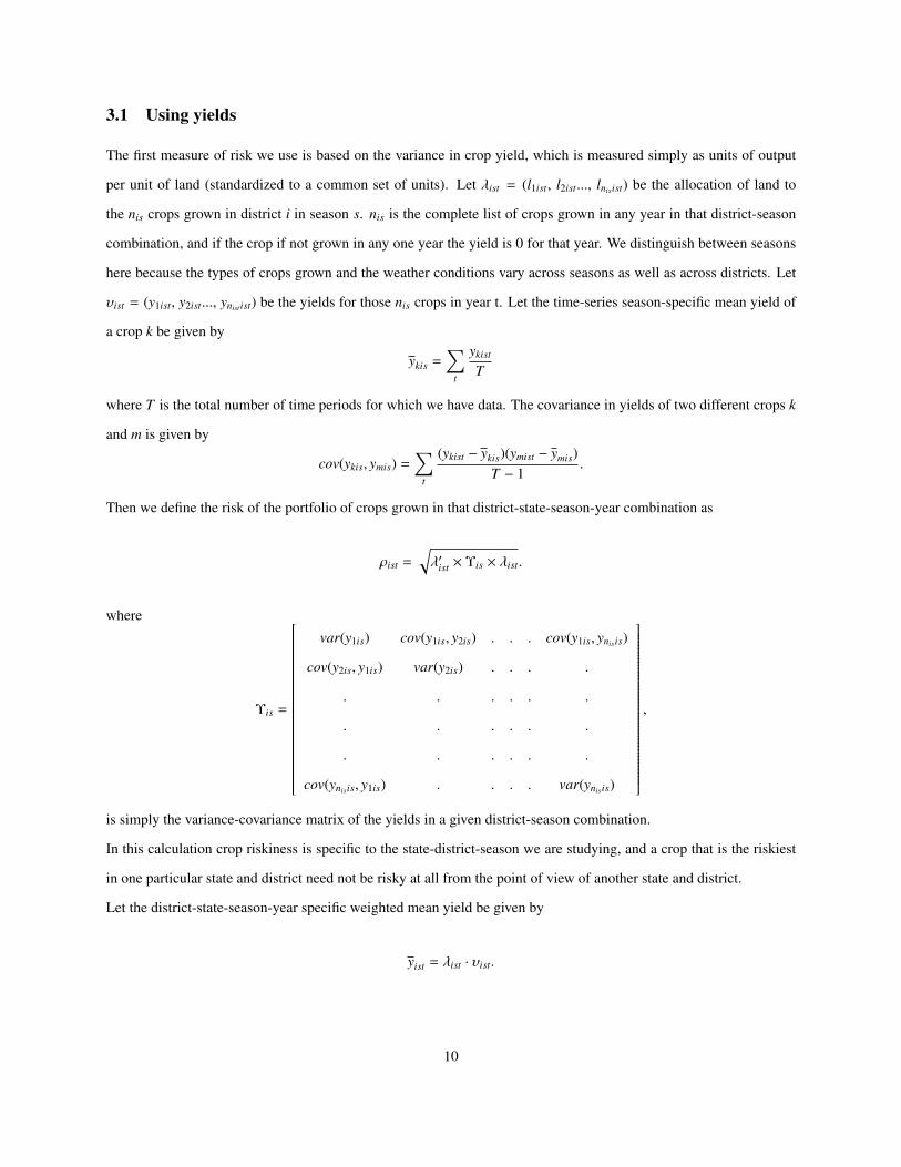
3.1 Using yields

The first measure of risk we use is based on the variance in crop yield, which is measured simply as units of output

per unit of land (standardized to a common set of units). Let �ist = (l1ist, l2ist..., lnisist) be the allocation of land to

the nis crops grown in district i in season s. nis is the complete list of crops grown in any year in that district-season

combination, and if the crop if not grown in any one year the yield is 0 for that year. We distinguish between seasons

here because the types of crops grown and the weather conditions vary across seasons as well as across districts. Let

�ist = (y1ist, y2ist..., ynist ist) be the yields for those nis crops in year t. Let the time-series season-specific mean yield of

a crop k be given by

ykis =X

t

ykist

T

where T is the total number of time periods for which we have data. The covariance in yields of two different crops k

and m is given by

cov(ykis, ymis) =X

t

(ykist � ykis)(ymist � ymis)T � 1

.

Then we define the risk of the portfolio of crops grown in that district-state-season-year combination as

⇢ist =q

�0ist ⇥ ⌥is ⇥ �ist.

where

⌥is =

2

6

6

6

6

6

6

6

6

6

6

6

6

6

6

6

6

6

6

6

6

6

6

6

6

6

6

6

6

6

6

6

6

6

6

6

6

6

6

6

6

6

6

6

6

4

var(y1is) cov(y1is, y2is) . . . cov(y1is, ynisis)

cov(y2is, y1is) var(y2is) . . . .

. . . . . .

. . . . . .

. . . . . .

cov(ynisis, y1is) . . . . var(ynisis)

3

7

7

7

7

7

7

7

7

7

7

7

7

7

7

7

7

7

7

7

7

7

7

7

7

7

7

7

7

7

7

7

7

7

7

7

7

7

7

7

7

7

7

7

7

5

,

is simply the variance-covariance matrix of the yields in a given district-season combination.

In this calculation crop riskiness is specific to the state-district-season we are studying, and a crop that is the riskiest

in one particular state and district need not be risky at all from the point of view of another state and district.

Let the district-state-season-year specific weighted mean yield be given by

yist = �ist · �ist.

10

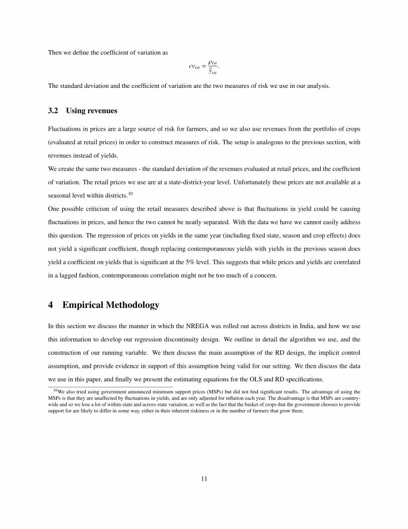
Then we define the coefficient of variation as

cvist =⇢ist

yist.

The standard deviation and the coefficient of variation are the two measures of risk we use in our analysis.

3.2 Using revenues

Fluctuations in prices are a large source of risk for farmers, and so we also use revenues from the portfolio of crops

(evaluated at retail prices) in order to construct measures of risk. The setup is analogous to the previous section, with

revenues instead of yields.

We create the same two measures - the standard deviation of the revenues evaluated at retail prices, and the coefficient

of variation. The retail prices we use are at a state-district-year level. Unfortunately these prices are not available at a

seasonal level within districts.10

One possible criticism of using the retail measures described above is that fluctuations in yield could be causing

fluctuations in prices, and hence the two cannot be neatly separated. With the data we have we cannot easily address

this question. The regression of prices on yields in the same year (including fixed state, season and crop effects) does

not yield a significant coefficient, though replacing contemporaneous yields with yields in the previous season does

yield a coefficient on yields that is significant at the 5% level. This suggests that while prices and yields are correlated

in a lagged fashion, contemporaneous correlation might not be too much of a concern.

4 Empirical Methodology

In this section we discuss the manner in which the NREGA was rolled out across districts in India, and how we use

this information to develop our regression discontinuity design. We outline in detail the algorithm we use, and the

construction of our running variable. We then discuss the main assumption of the RD design, the implicit control

assumption, and provide evidence in support of this assumption being valid for our setting. We then discuss the data

we use in this paper, and finally we present the estimating equations for the OLS and RD specifications.10We also tried using government announced minimum support prices (MSPs) but did not find significant results. The advantage of using the

MSPs is that they are unaffected by fluctuations in yields, and are only adjusted for inflation each year. The disadvantage is that MSPs are country-wide and so we lose a lot of within-state and across-state variation, as well as the fact that the basket of crops that the government chooses to providesupport for are likely to differ in some way, either in their inherent riskiness or in the number of farmers that grow them.

11

4.1 Program Roll-out and the Regression Discontinuity Design

The phased roll-out of the NREGA allows for the analysis of the causal effect of the program on a wide range of

outcomes. As mentioned earlier, many of the studies of the NREGA have used a difference-in-difference (DID)

approach to measure the impact of the Act on labor market outcomes. Such an approach is problematic as the program

was not introduced in a random manner and was in fact deliberately targeted at the poorest districts first. Many of

the earlier studies also use data which were collected after Phase 2 of the program was rolled out, meaning that they

can only compare Phase 2 and Phase 3 districts. Since many of the Phase 3 districts are some of the richest in the

country (and are from the richest or most developed states like Haryana, Punjab, Kerala, Tamil Nadu and Gujarat) the

common-trend assumption can be hard to defend. Indeed, Zimmermann (2013) provides evidence that it does not hold

for some outcomes.

Instead we use the fact that the NREGA was assigned to districts based on a poverty measure in order to develop

a regression discontinuity design that we believe is the most robust methodology for analyzing this program. The

poverty measure was based on data that pre-dated the NREGA by almost ten years, and was itself published two years

before the NREGA was announced (Planning Commission (2003a)).

Regression discontinuity essentially relies on a “jump” in treatment probabilities around a certain cut-off to identify

program impact. If treatment status is based on a certain cut-off, then units within a small range on either side of the

cut-off are likely to be similar on both observable and unobservable characteristics. For this small range around the

cut-off therefore, program assignment can be thought of as random.

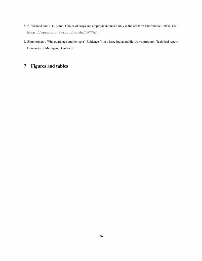
The NREGA program was first introduced in April 2006 in the poorest 200 districts in the country. In April 2007,

the next 130 poorest districts got the program. Finally, in April 2008 the program was introduced in all remaining

districts11. Figure 1 shows the phased roll-out of the program. Since the allocation was based on some poverty

measure (or measures) it lends itself to a regression discontinuity design, provided we can recover the ranking on

which this decision was based.

[FIGURE 1 ABOUT HERE.]

We use the information in Zimmermann (2013) to recover the algorithm used to rank the districts in order of poverty.

The actual treatment decision consisted of two stages. In the first stage the number of districts in each state to be

allocated the NREGA in the phase in question was determined on the basis of the proportion of people in that state

who were poor. In the second stage the exact identity of the districts to receive the program from each state was

determined on the basis of a ‘backwardness’ ranking, with the most backward districts within a state receiving the11India has a total of 655 districts, of which 30 are urban districts and hence did not receive the program in any wave of the roll-out.

12

program first.

The choice of the particular poverty measure employed for the first stage and the data on which the poverty calculation

was based are not publicly known. Zimmermann (2013) makes an educated guess at the criterion used. She uses the

poverty headcount ratio calculated from the 1993-1994 National Sample Survey (NSS) to calculate the “incidence of

poverty” for each state. Since the poverty measure is not known with certainty, we do not follow Zimmermann (2013)

in this first stage. Instead, we simply take the total number of districts allocated the program in a particular state as

given, and then proceed to the second stage.

In the second stage, districts within a state were ranked in terms of their backwardness, and the districts with the

highest rankings within each state received the program first. The ranking used for this purpose is publicly available

from Planning Commission (2003a), a report which provides a list of districts along with the calculation of an “Index

of Backwardness”. This is a composite index which assigns a score to each district along three dimensions - the

percentage of Scheduled Caste and Scheduled Tribe individuals in its population12 (from the 1991 census), agricultural

wages (from 1996-97), and the output per agricultural worker (from 1990-93). These three dimensions are then

aggregated to form a composite index for the district.

The Planning Commission ranking is available only for 447 districts in 17 states.13 Zimmermann (2013) suggests that

part of the reason for the omission of entire states might be because of “internal stability and security issues” during

the time that the data used in constructing the index was collected. As a result of this it is plausible that these states

played a larger role in determining which of their districts received the program, which would violate the implicit

control assumption of the regression discontinuity design. We simply omit those districts for which we do not have

information on the ranking.

One complication is that program allocation was not based entirely on these backwardness rankings. Broadly speaking,

two additional factors determined treatment. First, given the high variance in the backwardness index, some states,

e.g. Kerala, had no districts among the 200 most backward. Owing to political pressures, however, it was decided that

treatment would be made such that every state in India had at least one district which received the program in each

phase. Second, many districts in India are affected by the Maoist (an extremist left wing) movement. The government

viewed the NREGA as a tool to combat the influence of the Maoists and decided that all districts affected by the

movement would be assigned the NREGA in phase 1. These districts are in the states of Andhra Pradesh, Bihar,

Jharkhand, Madhya Pradesh, Chhattisgarh, Orissa and Uttar Pradesh. The list of 32 ‘extremist affected districts’ is

available in Planning Commission (2003b).12These are two groups of historically disadvantaged individuals that are formally recognized by the Constitution of India.13India has a total of 29 states and 7 union territories. The 17 states for which the ranking is available are the most populous states, however, and

according to 2011 Census data they make up 94.66% of India’s population.

13

Using these elements of the NREGA program design, we construct an algorithm that predicts program assignment and

use this to implement our RD strategy. The program prediction algorithm works as follows:

• Step 1: Rank districts within a state s using the Backwardness Index published by the Planning Commission.

• Step 2: Take the total number of NREGA districts actually assigned to a state s, ns, as given. Allocate the

available ns slots starting with the most backward district in the state receiving the program first.

• Step 3: Create state-normalized ranks by assigning the most backward district in a state a rank of �ns, the

second-last district the rank of �ns + 1 and so on, such that the district with state-normalized rank of 0 is the last

district predicted to receive the NREGA in each state.

The construction of the state-normalized rank ensures that the discontinuity is evaluated at a common point across

states, in this case at the value 0. The state-normalized rank is the ‘running variable’ in our regression discontinuity

design, i.e., the numerical variable which predicts the probability of treatment.

Clearly this process can be performed so as to generate cut-offs for both phases, but we focus for now on the Phase 1

cut-off. This is because we believe that districts in Phases 1 and 2 were more similar to each other than Phase 1 and 2

districts were to Phase 3 districts, so the comparison of cropping choices along this boundary is more justifiable. By

construction, districts with negative state-normalized ranks are predicted to have received the program, and districts

with strictly positive state-normalized ranks are predicted to not have got it. If we restrict attention to a small enough

bandwidth around the cut-off of 0, treatment prediction can be thought of as being random since districts have similar

backwardness index scores, but differ in treatment status. Alternatively, we can expand our bandwidth around the

cut-off and use a flexible polynomial specification. Since the number of districts and state-normalized ranks is small,

we prefer to use all districts without restricting our attention to a bandwidth. We present robustness checks which

exclude Phase 3 districts, and employ a number of different specifications.

[TABLE 1 ABOUT HERE.]

How well does the algorithm do in predicting program allocation? Table 1 gives a state-wise break-up of the actual

number of districts assigned the NREGA in Phase 1 and the algorithm prediction success. As is clear from the table,

the algorithm performs better in some states than in others. The overall probability of success in prediction is 80%.

The table also reports the number of false negatives - i.e. the number of districts our algorithm predicts as not having

received the program that did in fact actually receive the program in Phase 1.


14

Given the imperfect prediction of program assignment - the cut-off of 0 does not predict actual treatment determin-

istically - we use a fuzzy RD design. Figure 2 plots the mean probability of receiving the program for each state-

normalized rank. The fitted curves are quadratic, with 95% confidence intervals plotted as well. The 95% confidence

intervals do not overlap, though the discontinuity is not very clear.


One of the steps that was followed in the actual assignment of the program was to allocate the program to all 32

‘extremist’ districts regardless of their ranking in the Planning Commission Backwardness index. The 32 extremist

districts were not always among the lowest ranked districts in their states. Often these districts were close to the

state-specific cut-off, but sometimes they were significantly more ‘advanced’. Not taking this into account while

reconstructing the algorithm results in a greater probability of incorrect assignment around the cut-off of 0 that visibly

dampens the discontinuity at this point. To demonstrate this we also present the graph of the fuzzy RD without the

inclusion of the extremist districts (see Figure 3). As can be seen from this figure, the discontinuity is much stronger

at the cut-off point. We thus also present results for the sample without the extremist districts.

4.2 Possible Concerns

One of the concerns with any RD design is potential manipulation of the assignment variable by the beneficiaries of

the program. Since treatment is on the basis of a cut-off, if units could slightly misreport or manipulate their scores

then the “quasi-randomness” of allocation around the cut-off would no longer hold. In our case, this means that if it

were possible for districts to misreport their scores on the backwardness index, then we would be worried that districts

on either side of the cut-off systematically differ on unobservable characteristics such as potential benefits from the

program or political influence.

This is unlikely to be the case for the NREGA. Firstly, the data used for construction of each of the dimensions of

the backwardness index comes from the mid-1990s, so it pre-dates the introduction of the NREGA by approximately

10 years. Secondly, the same ranking had been used previously for the allocation of other welfare programs, but with

different cut-offs of 100 or 150 districts. So even if districts could manipulate their ranks, there is no reason to think

that they would know to aim for the NREGA cut-off of 200 districts in Phase 1.


To further demonstrate that the districts did not have control over their ranking, Figure 4 depicts the relationship

between the backwardness index score and the overall district ranks (which range from 1 to 447). If there was strategic

15

misreporting we would expect to see clustering just below the cut-offs of 200 (Phase 1) and 330 (Phase 1 and 2

together), which does not seem to be the case. As can be seen from the graph, the relationship is smooth, with a

couple of inflection points where the curve becomes flatter or steeper. These inflection points are at around 100 and

400 districts respectively. The backwardness index score ranges from 0.08 to 2.3.


Finally, Figure 5 depicts state-wise graphs of the state-normalized rank versus the composite ranking of districts. In

this graph, discontinuities around the normalized cut-off of 0 would be suggestive of manipulation on the part of

individual states. We do not see any evidence of such discontinuities.

The evidence presented above gives us confidence in the fact that the individual districts did not have control over their

scores in the Backwardness Index.

4.3 Data

The information needed to recreate the algorithm for the district assignment of NREGA comes from the Planning

Commission (2003a). This document provides the score of each of the 447 districts on each of the three indicators

- agricultural wages, percentage of the population that is made up of SC/ST individuals and output per agricultural

worker, the composite score which is a combination of these three scores, and then the ranking of the districts according

to the composite score. As described above we use the ranking of districts in this document to create the running

variable of our RD, the state-normalized rank.

Information on crop yields, land use and season comes from a dataset published by the Ministry of Agriculture,

Government of India. This dataset is a district level panel for the years 1998 to 2010, and provides information on area

under cultivation and total production for each crop grown in all districts in India, across rabi, kharif, autumn, winter

and summer seasons of the year. The number of crops varies across districts in a given year and season, across years

within a particular district and season, and across seasons within a particular district-year combination. Data on crop

production is in metric tons and on land use is in hectares (ha).

The price data used is retail prices for the period 2001-2010 from the Retail Prices Information System, Directorate

of Economics and Statistics, Department of Agriculture and Cooperation, Ministry of Agriculture, Government of

India14. The price data is at a sub-state regional level. More accurate measures of district level prices might match dis-

tricts with the closest available regional price value, but without any way of analyzing the distance between individual

districts and the regional focal point we simply aggregate the information to a state level. All prices have been deflated14This data is available at http://rpms.dacnet.nic.in/Bulletin.aspx

16

using the Consumer Price Index (CPI), and are evaluated at a 1986-87 base. The CPI is available at a state-year level.

We calculate the simple mean of the prices for a particular state-crop-year combination and use that number for every

district within the state. We should mention here that the price data is limited and covers only about a third of the

crops in our sample. We have been unable to find information on other crops from other sources.

We have also tried using government minimum support prices (MSPs) instead of retail prices. The MSPs are available

for an even smaller number of crops than the retail price information, and are also centrally-announced prices and so

do not vary by state. Using the MSPs does not give us any significant results for revenues. The results with MSPs are

not reported here.

4.4 Empirical Methodology

4.4.1 OLS estimates

We start with the specification for the OLS estimates of the effect of being a district with the NREGA on the risk-taking

behavior of farmers. The main equation we use is as follows. For a district i in state j in season s and year t:

Outcomeist = ↵ + �NREGAit + �t + �s + � j + "ist (1)

Outcomeist is the outcome of interest - the standard deviation or coefficient of variation of revenue or yield for district i

in state j in season s in time t, NREGAit is a dummy which takes the value 1 if the district was assigned to the NREGA

program in year t. The equation includes a linear time trend and state and season fixed effects. Different versions of

the results are presented with different combinations of the above covariates, and often include as well the level of

previous risk from the year prior as a control.

4.4.2 Regression discontinuity estimates

The most flexible form of the main equation of interest is:

Outcomeist = ↵ + � gNREGAit + �ranki j + �rank2i j + ⌘

gNREGAitranki j (2)

+� gNREGAitrank2i j + µ j + �s + ✓Baselineis + "ist

where Outcomeist is the dependent variable in district i during season s ; gNREGAit is a dummy variable taking the

value 1 if the program is predicted to have been introduced in phase 1 in district i in year t; Ranki is the state normalized

rank for district i; Baselineis is the value of the dependent variable in the same season of the previous year; µ j are state

17

fixed effects, and �s are season fixed effects.

In this specification, we allow for the regression slopes and intercepts to vary on either side of the treatment cut-offs.

The coefficient of interest is �, which is the intent-to-treat (ITT) estimate of the program. We vary this specification

and present results for four variants - a linear form on either side of the cut-off, a linear flexible form with slopes

allowed to vary, a quadratic form and then finally the quadratic flexible form of the equation above. Each of the other

specifications is simply a special case of the quadratic flexible form, and so the latter is our preferred specification,

even though we present results from all four equations.

The dependent variable is the chosen measure of risk. In the above specification the main variable of interest is the

dummy for whether or not the district got the program in phase1, NREGAit. This captures the jump in risk-taking

behavior at the normalized cut-off of 0.

4.4.3 Theoretical decomposition of land reallocations

The last set of tests we conduct is to check whether the manner in which districts reallocate their land changes after

the introduction of the NREGA. The basic specification we use for this is the same as in equation 2. The outcomes of

interest are the total amount of ‘churning’ or changes in crop land allocation, the quantity of land that was reallocated

in order to increase risk, and the quantity of land that was reallocated in order to decrease risk. The theoretical

justification for using this measure and the results of the decomposition are in the Appendix.

5 Results

In this section we present results for both the OLS and the RD specifications, with various different outcome variables.

All the results we present here exclude Phase 3 districts entirely, and focus only on Phase 1 and 2 districts. The Phase 3

districts are the richest in the country and received the program last. It is harder to argue, therefore, that these districts

are comparable to districts that received the program in the first or second phases. Phase 3 districts will be included in

the robustness checks, and we will show that their inclusion does not alter our results significantly.

5.0.1 Average yields and revenues

Tables 2 and 3 present regression discontinuity results for average portfolio yields and average portfolio revenues in

the post-program period in 2007. As a reminder, the average portfolio yield is given by:

yist = �ist · �ist.

18

The average portfolio revenue is calculated analogously.

[TABLES 2 AND 3 ABOUT HERE.]

As can be seen from Tables 2 and 3, there is no significant difference between districts that were predicted to receive

the program and those that were not, in terms of the average returns to the portfolio of crops. A priori we would expect

that riskier crops should also be higher return crops, so that if we see an increase in the riskiness of the portfolio then

we should also see an increase in the mean return. That hypothesis cannot be rejected with the evidence presented here.

The portfolio of crops in districts that were predicted to receive the program do not seem to be generating significantly

higher average returns, at least in 2007.

[TABLE 4 ABOUT HERE.]

Though we cannot show that districts do indeed earn higher average returns from their portfolios, we can show in

a very simple manner that portfolios that are riskier are associated with higher returns. Table 4 presents the simple

correlations between the district crop portfolio risk (measured by the standard deviation) and its return, as calculated

by using the yields and the revenues at retail prices for the two major agricultural seasons. The returns and risk are

indeed positively correlated, suggesting that portfolios with greater risk on average have greater mean returns as well.

5.0.2 OLS results

To begin with, we present the results for the OLS specification from equation 1. Tables 5 and 6 present the results for

the standard deviations of both yields and revenues. In these specifications, NREGAit is a dummy that takes on value

1 if the district i in state j received the NREGA in time t. Since the districts that received the program were poorer to

begin with, we should expect that the estimates on the receipt of the NREGA should be biased downward, giving us

smaller results than we would get in the case of the regression discontinuity.


We restrict the sample to the years 1998 to 2007, and remove all Phase 3 districts from consideration. As can be seen

from the tables, there is a strong significant effect of the NREGA dummy on the measures of risk employed, in the

case of both revenues and yields. In fact the OLS results are indeed smaller than the RD estimates for the sample

without Phase 3 districts, as will be seen in the next section.

19

5.0.3 Regression Discontinuity Results

In this section we present the results from the regression discontinuity estimating equation presented in Section 4

above. We begin with the sample that includes the extremist districts, and present results that use all districts with-

out restricting attention to a specific bandwidth around the cut-off. All tables include lagged values of the relevant

dependent variable, and fixed state and season effects. Since we are using the entire sample, we employ different

specifications and allow for flexibility in slope and intercept in order to try to capture as best as possible the behavior

of the data.


Tables 7 and 8 present the baseline results for the year 2005 before the program was introduced in any of the districts.

These results include extremist districts, but exclude the richest districts that got the program in Phase 3. We should

expect that there be no significant differences between districts on the yield or revenue risk measures prior to the

introduction of the program. For both yields and revenues, the coefficient on the predicted assignment of NREGA

variable is positive, however it is not statistically significant.

Thus there does seem to be evidence that the Phase 1 and 2 districts were not significantly different from one another

in terms of risk-taking behavior prior to the introduction of the NREGA.


The next set of tables, Tables 9 and 10, present the results for the year 2007 for both yields and revenues. We see an

increase in the standard deviation of yields and revenues that is large, and persists across all specifications. Are the

numbers for revenue increases reasonable? When we restrict our attention to the crops for which we have information

on prices (table not shown here), the coefficients on NREGA receipt for increases in the standard deviation of yields

range from .726 to 1.043 tons per hectare. These evaluated at the mean price of Rs. 5096.25 per ton (1000 kg) yield

increases in the standard deviation of revenues in the range of Rs. 3700 to Rs. 5300 per hectare, which is comparable

to the coefficients presented here. The numbers for the increase in the standard deviations of revenues are larger than

this range, but given the dispersion in the price distribution the numbers are not unreasonable. Also, the numbers

for the increase in the standard deviation of revenues seem large, but one should remember that these are per 10,000

square meters, and are not the measures of increases in the standard deviations of profits since we do not have cost of

cultivation information.


20

When the extremist districts are excluded from the sample, the OLS results of the effect of the introduction of the

NREGA on the standard deviation of yields and revenues continue to show positive significant coefficients across

almost all specifications (as can be seen from Tables 11 and 12).

[FIGURES 6, 7, 8 AND 9 ABOUT HERE.]

Figures 6 to 9 plot graphically the coefficient of variation of revenues and yields (with extremist districts included) for

the baseline and for the post-program periods. The graphs look very similar in shape, though not in scale. The vertical

line is at the cut-off point for the allocation of the program. The baseline pictures do not show any discontinuities at

the cut-off. The graphs for the year 2007 do, but the discontinuity is not as clear as one would have hoped for.

[TABLES 13, 14, 15 AND 16 ABOUT HERE.]

Tables 13 and 14 present the same RD baseline results but for the sample where the set of extremist districts has been

excluded, and the state-normalized rank calculated accordingly. Again we see no differences in the districts prior to the

introduction of the program. However, the results for the year 2007 presented in Tables 15 and 16 show no significant

results. The magnitudes of the coefficients are very similar to the results with extremist districts, and there is a positive

effect on risk-taking in all four tables, though the standard errors have increased so that none of the changes appear

significant.

The change in the results when the extremist districts are excluded might simply be a result of the fall in the size

of the sample, or it might be because of something specific to the extremist districts. If these are districts where the

government is already investing more resources in order to appease the rebel groups, then there may be other programs

going on at the same time that are driving greater increases in the risk of the crop portfolios than in other districts.

5.1 Robustness

All of the above results present estimates for the sample that excludes Phase 3 districts entirely. Just to show that the

inclusion of these districts does not have any impact on the results, in the Appendix we present similar tables with

Phase 3 districts included. These tables are in the same format as the ones in the main results section.

In addition, we have tables for the other two measures of risk that we discussed above, and also results for the same

specifications but with the sample restricted to the set of crops for which we have price information.

As can be seen from the tables in the Appendix (tables 17 to 22) the quantitative results are mainly unchanged.

The introduction of the NREGA still seems to have increased risk-taking behavior, though statistical significance has

declined somewhat. Most of the changes in the results for the year 2007 show the same pattern as before, with the

21

results on revenues being significant in the majority of the specifications. In addition, when we restrict our attention

only to the yields of those crops for which we have price information (Tables 21 and 22) we see that the standard

deviation of the yield has increased. This result holds whether or not we include the Phase 3 districts.

Our results are not completely robust, but within the limitations of the dataset we have we show that at least some of

the main conclusions hold even when the sample is changed and the estimation methods are altered.

5.2 Impact of the NREGA on formal credit

While it seems fairly clear that the NREGA has had an effect on the riskiness of the portfolios of crops being grown at

a district level, we have as yet been unable to pinpoint the exact channel through which this operates. One possibility

is the relaxation of credit constraints. Using data on formal credit, we estimated the impact of NREGA on loan take

up, and found no impact. This may not be very surprising, given that formal credit is a small share of the total credit

small and marginal farmers have access to. On the other hand, data on informal credit is very hard to obtain. Using

data from a field survey in West Bengal, Dey (2010) finds that informal loans (as measured by credit given by small

grocers and shop keepers) has gone up as in response to the program. It would be interesting to see if this finding holds

for other parts of India.

6 Conclusion

The NREGA is an ambitious, large scale employment guarantee program. While the focus of the program from a

policy maker’s point of view has been on the higher incomes and employment generated, as well as the public works

built using labor supplied under the program, the NREGA can affect the rural economy in several other ways. In this

paper we studied the role of the program in providing insurance or reducing credit constraints.

Our main contribution has been to look at changes in crop-choice across the country as a result of the introduction of

this program. We use a regression-discontinuity design, which we believe is one of the more robust ways of causally

estimating the causal effect of the NREGA. We also provide a theoretical decomposition measure that divides total

changes in land allocation into those that increase risk and those that reduce it. The data on crop yields is limited,

and our methodology cannot identify the exact mechanism that is driving the increase in risk-taking. In particular we

do not know if the main impact of the NREGA operates through the relaxation of credit constraints, or through the

provision of insurance. We find that the amount of risk in the district-level crop portfolios has increased as a result of

the introduction of the program, suggesting that the program might well be easing one or both of these constraints.

In order to try to disentangle credit constraints from the role of uninsured risk we looked at the effect of the NREGA

22

on the total changes in land allocation. We find no increase in the total number of changes in land allocation, which

suggests that the reason farmers are not changing their cropping patterns might have less to do with there being a fixed

cost to adoption, and more to do with uninsured risk.

References

M. Azam. The Impact of Indian Job Guarantee Scheme on Labor Market Outcomes: Evidence from a Natural Ex-

periment. Technical report, IZA Discussion Paper Series 6548, May 2012. URL http://www.iza.org/en/

webcontent/publications/papers/viewAbstract?dp id=6548.

E. Berg, S. Bhattacharyya, R. Durgam, and M. Ramachandra. Can rural public works affect agricultural wages? Evi-

dence from India. CSAE Working Paper, May 2012. URL http://www.csae.ox.ac.uk/workingpapers/

pdfs/csae-wps-2012-05.pdf.

A. K. Bhargava. The impact of India’s rural employment guarantee on demand for agricultural technology. Technical

report, IFPRI Discussion Paper, July 2014. URL http://akbhargava.weebly.com/uploads/2/1/2/5/

21256332/akb 2014-07-15.pdf.

A. Case, A. Garrib, A. Menendez, and A. Olgiati. Paying the piper: The high cost of funerals in South Africa.

Economic Development and Cultural Change, 62(1), 2013.

P. Chakraborty. Implementation of the National Rural Employment Guarantee Act in India: Spatial dimensions and

fiscal implications. Technical report, National Institute of Public Finance and Policy and The Levy Economics

Institute of Bard College, 2007.

S. Dercon and L. Christiaensen. Consumption risk, technology adoption and poverty traps: Evidence from Ethiopia.

Journal of Development Economics, 96:159–173, 2011.

S. M. Dev. Small farmers in India: Challenges and opportunities. Technical report, Indira Gandhi Institute of Devel-

opment Research, 2012. URL http://www.igidr.ac.in/pdf/publication/WP-2012-014.pdf.

S. Dey. Evaluating the impact of the National Rural Employment Guarantee Scheme: The case

of Birbhum district, West Bengal, India. Technical report, International Institute of Social Studies,

The Hague, January 2010. URL http://www.iza.org/en/webcontent/publications/papers/

viewAbstract?dp id=6548. ISS Working Paper No. 490.

23

P. Dutta, R. Murgai, M. Ravallion, and D. van de Walle. Does India’s employment guarantee scheme guarantee

employment? Technical report, 2012. World Bank Policy Research Working Paper 6003.

M. Fafchamps and J. Pender. Precautionary saving, credit constraints, and irreversible investment: Theory and evi-

dence from semiarid India. Journal of Business & Economic Statistics, 15(2):180–194, 1997.

A. D. Foster and M. R. Rosenzweig. Microeconomics of technology adoption. Annual Review of Economics, 2(1):

395–424, 2010.

E. Gehrke. An employment guarantee as risk insurance? Assessing the effects of the NREGS on agricultural produc-

tion decisions. Technical report, BGPE Discussion Paper No. 152, May 2014. URL http://www.die-gdi.de/

uploads/media/152\ Gehrke.pdf.

X. Gine and S. Klonner. Credit constraints as a barrier to technology adoption by the poor. Research Paper 2006/104,

UNU-WIDER, September 2006.

M. Grimm, R. Hartwig, and J. Lay. Investment decisions of small entrepreneurs in a context of strong sharing norms.

Workng paper, World Bank Social Protection and Laor, October 2011.

C. Imbert and J. Papp. Government Hiring and Labor Market Equilibrium: Evidence from India’s Employment

Guarantee. Presented at the ISI conference, New Delhi, December 2011. URL http://www.isid.ac.in/

\˜

pu/conference/dec\ 11\ conf/Papers/ClementImbert.pdf.

C. Imbert and J. Papp. Labor market effects of social programs: Evidence from India’s employment guarantee.

Technical report, Centre for the Study of African Economies, University of Oxford, 2013. CSAE Working Paper

Series 2013-03.

D. Johnson. Can Workfare serve as a Substitute for Weather Insurance? The Case of NREGA in Andhra Pradesh.

Technical report, Institute for Financial Management and Research, Centre for microfinance, 2009. URL http:

//ifmr.ac.in/cmf/publications/wp/2009/32\ Johnson\ NREGA\ Bad\%20Weather.pdf.

D. Karlan, R. Osei, I. Osei Akoto, and C. Udry. Agricultural decisions after relaxing credit and risk constraints. The

Quarterly Journal of Economics, 129(2):597–652, 2012.

E. Ligon, J. P. Thomas, and T. Worrall. Informal insurance arrangements with limited commitment: Theory and

evidence from village economies. The Review of Economic Studies, 69(1):209–244, 2002.

24

O. Mahul, N. Verma, and D. J. Clarke. Improving farmers’ access to agricultural insurance in India. Working paper

no. 5987, The World Bank, March 2012. URL http://elibrary.worldbank.org/doi/pdf/10.1596/

1813-9450-5987.

A. M. Mobarak and M. Rosenzweig. Selling formal insurance to the informally insured. Working paper, Yale Univer-

sity, 2014.

J. Morduch. Risk, production, and saving: Theory and evidence from Indian households. Unpublished, Harvard

University, 1990.

C. M. Moser and C. B. Barrett. The complex dynamics of smallholder technology adoption: The case of SRI in

Madagascar. Agricultural Economics, 35:373–388, 2006.

K. Munshi and M. Rosenzweig. Networks and misallocation: Insurance, migration and the rural-urban wage gap.

Working paper, October 2013.

P. Niehaus and S. Sukhtankar. Corruption Dynamics: The Golden Goose Effect. American Economic Journal:

Economic Policy, 5(4):230–69, 2013.

Planning Commission. Report of the Task Force: Identification of districts for wage and self-employment pro-

grammes. Technical report, 2003a.

Planning Commission. Backward Districts Initiative - Rashtriya Sam Vikas Yojana - the Scheme and Guidelines for

preparation of District Plans. Technical report, 2003b. MLP division.

M. Rosenzweig. Risk, implicit contracts and the family in rural low-income countries. Working paper, Economic

Development Center, University of Minnesota, November 1986.

M. Rosenzweig and H. Binswanger. Wealth, Weather risk and the composition and profitability of agricultural invest-

ments. The Economic Journal, 103(416):56–78, 1993.

M. Rosenzweig and O. Stark. Consumption smoothing, migration, and marriage: Evidence from rural India. Journal

of Political Economy, 97(4):905–926, 1989.

K. J. S. Satyasai. Access to rural credit and input use: An empirical study. Agricultural Economics Research Review,

Conference Number:461–471, 2012.

R. M. Townsend. Risk and insurance in village India. Econometrica, 62(3):539–91, 1994.

25

S. N. Wadood and R. L. Lamb. Choice of crops and employment uncertainty in the off-farm labor market. 2006. URL

http://mpra.ub.uni-muenchen.de/10779/.

L. Zimmermann. Why guarantee employment? Evidence from a large Indian public-works program. Technical report,

University of Michigan, October 2013.

7 Figures and tables

26

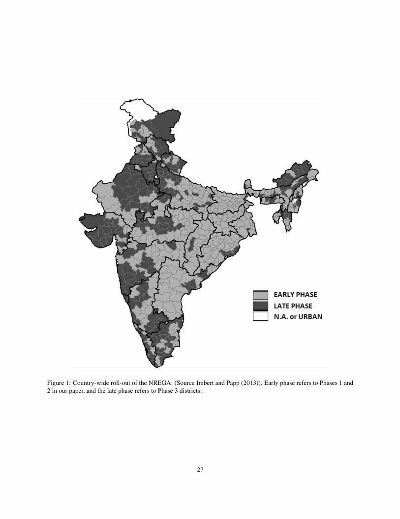
Figure 1: Country-wide roll-out of the NREGA: (Source Imbert and Papp (2013)). Early phase refers to Phases 1 and2 in our paper, and the late phase refers to Phase 3 districts.

27

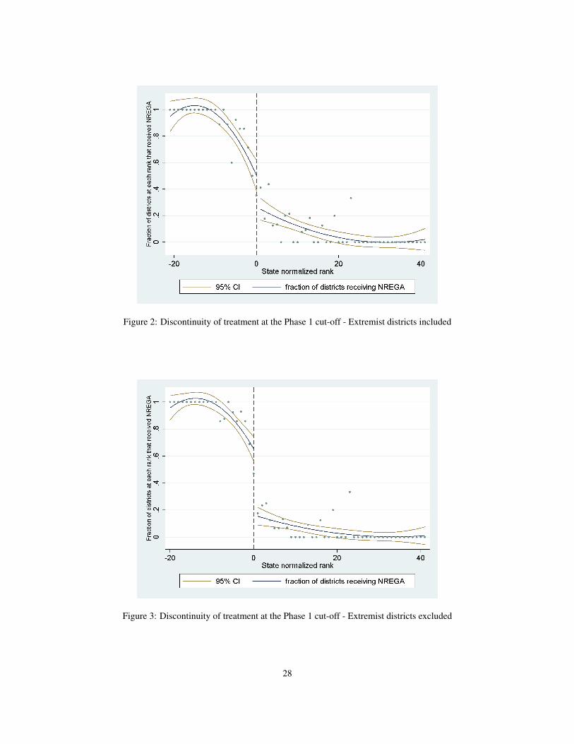
Figure 2: Discontinuity of treatment at the Phase 1 cut-off - Extremist districts included

Figure 3: Discontinuity of treatment at the Phase 1 cut-off - Extremist districts excluded

28

Figure 4: The composite score on the Backwardness Index vs. the overall district ranking (Source: Planning Commis-sion (2003a))

Figure 5: The composite score vs. the state-normalized rank. Each symbol refers to a particular state.

29

Figure 6: Standard deviation of yield - baseline (2005)

Figure 7: Standard deviation of yield - endline (2007)

30

Figure 8: Standard deviation of revenues - baseline (2005)

Figure 9: Standard deviation of revenues - endline (2007)

31

Table 1: Algorithm Success Rate for Phase 1

State Phase 1districts

Correctlypredicted

False neg-atives

Non-phase 1districts

False neg.rate (%)

Success(%)

Andhra Pradesh 13 10 3 8 37.5 76.9Assam 7 7 0 16 0 100.0Bihar 22 16 6 14 42.8 72.7Chhattisgarh 11 9 2 4 50 81.8Gujarat 6 4 2 14 14.3 66.7Haryana 2 0 2 16 12.5 0.0Jharkhand 18 17 1 2 50 94.4Karnataka 5 4 1 21 4.7 80.0Kerala 2 1 1 11 9 50.0Madhya Pradesh 18 13 5 24 20.8 72.2Maharashtra 12 11 1 18 5.6 91.7Orissa 19 17 2 11 18.1 89.5Punjab 1 1 0 14 0 100.0Rajasthan 6 5 1 25 4 83.3Tamil Nadu 6 4 2 20 10 66.7Uttar Pradesh 22 19 3 41 7.3 86.4West Bengal 10 8 2 7 28.6 80.0

Total 180 146 34 266 12.8 80.0Note: Because of the design of our prediction model, which always has exactly as many predicted phase 1 districts aswere allocated to the state, the number of false negatives always equals the number of false positives, although they aredifferent districts. The false positive rate, which is not presented in the table, equals False negatives/Phase 1 districts.

Table 2: Effect of the NREGA on average portfolio returns in 2007 (yields)

Dependent variable: Average portfolio yieldsSpecification Linear Lin. Flex. Quadratic Quad. Flex.gNREGAit 0.652 0.618 0.655 0.905

(0.52) (0.53) (0.52) (0.71)Lagged risk Yes Yes Yes YesState FE Yes Yes Yes YesSeason FE Yes Yes Yes Yes

Observations 949 949 949 949* p < 0.10, ** p < 0.05, *** p < 0.01. Robust standard errors in parentheses.

32

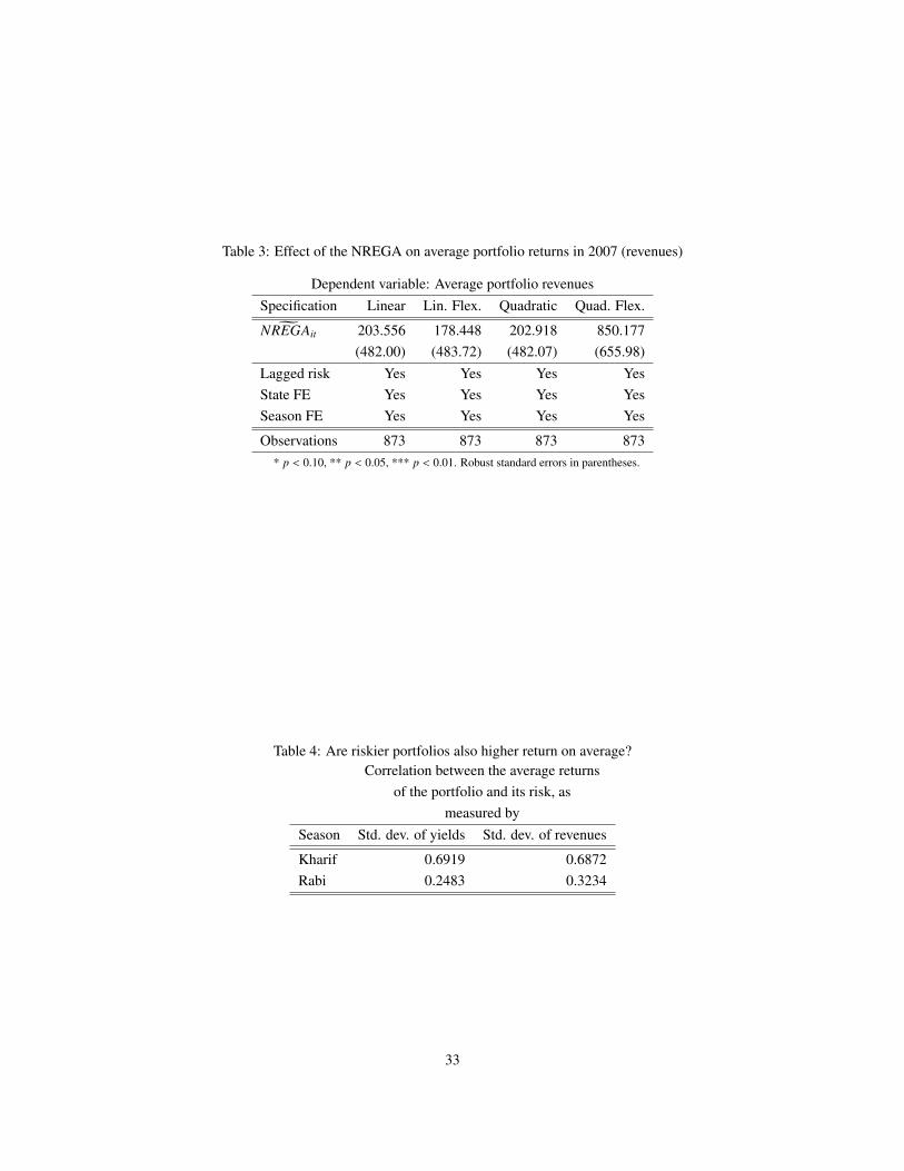
Table 3: Effect of the NREGA on average portfolio returns in 2007 (revenues)

Dependent variable: Average portfolio revenuesSpecification Linear Lin. Flex. Quadratic Quad. Flex.gNREGAit 203.556 178.448 202.918 850.177



Table 4: Are riskier portfolios also higher return on average?Correlation between the average returns

of the portfolio and its risk, asmeasured by

Season Std. dev. of yields Std. dev. of revenues

Kharif 0.6919 0.6872Rabi 0.2483 0.3234

33

Table 5: Effect of NREGA on riskiness (std. dev. of yields) - OLS results

Dependent Variable: Standard deviation of yields

NREGA 0.443* 0.519** 0.594** 0.632** 0.274 0.299(0.242) (0.242) (0.257) (0.258) (0.323) (0.325)

Previous risk No Yes No Yes No YesSeason FE No No Yes Yes Yes YesState FE No No Yes Yes Yes YesTime trend No No No No Yes Yes

Observations 8928 8928 8928 8928 8928 8928* p < 0.10, ** p < 0.05, *** p < 0.01. Robust standard errors in parentheses.

Table 6: Effect of NREGA on riskiness (std. dev. of revenues) - OLS results

Dependent Variable: Standard deviation of revenues (in Rs. ‘000s)

NREGA 4.331 6.712** 6.716* 8.319** 3.684 2.896(3.310) (3.236) (3.491) (3.467) (5.679) (5.728)

Previous risk No Yes No Yes No YesSeason FE No No Yes Yes Yes YesState FE No No Yes Yes Yes YesTime trend No No No No Yes Yes


34

Table 7: Effect of NREGA on riskiness (std. dev. of yields) - RD results in 2005

Dependent variable: Standard deviation of yieldsSpecification Linear Lin. Flex. Quadratic Quad. Flex.gNREGAit 0.003 0.004 0.003 0.000



Table 8: Effect of NREGA on riskiness (std. dev. of revenues) - RD results in 2005

Dependent variable: Standard deviation of revenues (in Rs. ‘000s)Specification Linear Lin. Flex. Quadratic Quad. Flex.gNREGAit .031 .030 .031 .005

(.029) (.029) (.029) (.039)Lagged risk Yes Yes Yes YesState FE Yes Yes Yes YesSeason FE Yes Yes Yes Yes


Table 9: Effect of NREGA on riskiness (std. dev. of yields) - RD results in 2007

Dependent variable: Standard deviation of yieldsSpecification Linear Lin. Flex. Quadratic Quad. Flex.gNREGAit 0.363* 0.349* 0.363* 0.580**



35

Table 10: Effect of NREGA on riskiness (std. dev. of revenues) - RD results in 2007

Dependent variable: Standard deviation of revenues (in Rs. ‘000s)Specification Linear Lin. Flex. Quadratic Quad. Flex.gNREGAit 5.561* 5.411* 5.569* 7.920*



Table 11: Effect of NREGA on riskiness (std. dev. of yields) - OLS results, no extremist districts

Dependent Variable: Standard deviation of yields

NREGA 0.364 0.439* 0.503** 0.540** 0.196 0.220(0.230) (0.230) (0.240) (0.241) (0.309) (0.310)

Previous risk No Yes No Yes No YesSeason FE No No Yes Yes Yes YesState FE No No Yes Yes Yes YesLinear time trend No No No No Yes Yes


Table 12: Effect of NREGA on riskiness (std. dev. of revenues) - OLS results, no extremist districts

Dependent Variable: Standard deviation of revenues (in Rs. ‘000s)

NREGA 1.517* 1.516* 1.603* 1.588* 1.294* 1.281*(.854) (.851) (.895) (.876) (.715) (.698)

Previous risk No Yes No Yes No YesSeason FE No No Yes Yes Yes YesState FE No No Yes Yes Yes YesLin. time trend No No No No Yes Yes


36

Table 13: Effect of NREGA on riskiness (std. dev. of yields) - RD results in 2005, no extremist districts

Dependent Variable: Standard deviation of yieldsSpecification Linear Lin. Flex. Quadratic Quad. Flex.gNREGAit -0.001 -0.000 -0.002 -0.010



Table 14: Effect of NREGA on riskiness (std. dev. of revenues) - RD results in 2005, no extremist districts

Dependent Variable: Standard deviation of revenue (in Rs. ‘000s)

Specification Linear Lin. Flex. Quadratic Quad. Flex.gNREGAit -.013 -.013 -.013 -.012

(.010) (.010) (.010) (.014)Lagged risk Yes Yes Yes YesState FE Yes Yes Yes YesSeason FE Yes Yes Yes Yes


Table 15: Effect of NREGA on riskiness (std. dev. of yields) - RD results in 2007, no extremist districts

Dependent Variable: Standard deviation of yieldsSpecification Linear Lin. Flex. Quadratic Quad. Flex.gNREGAit 0.319 0.287 0.327 0.376



37

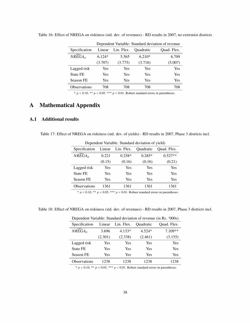
Table 16: Effect of NREGA on riskiness (std. dev. of revenues) - RD results in 2007, no extremist districts

Dependent Variable: Standard deviation of revenueSpecification Linear Lin. Flex. Quadratic Quad. Flex.gNREGAit 6.124* 5.565 6.210* 6.709



A Mathematical Appendix

A.1 Additional results

Table 17: Effect of NREGA on riskiness (std. dev. of yields) - RD results in 2007, Phase 3 districts incl.

Dependent Variable: Standard deviation of yield)Specification Linear Lin. Flex. Quadratic Quad. Flex.gNREGAit 0.221 0.258* 0.285* 0.527**



Table 18: Effect of NREGA on riskiness (std. dev. of revenues) - RD results in 2007, Phase 3 districts incl.

Dependent Variable: Standard deviation of revenue (in Rs. ‘000s)Specification Linear Lin. Flex. Quadratic Quad. Flex.gNREGAit 3.696 4.133* 4.524* 7.109**



38

A.2 Results with other measures of risk

Table 19: Effect of NREGA on riskiness (coeff. of var. of yields) - RD results in 2007, Phase 3 districts excl.

Dependent Variable: Coefficient of variation of yieldSpecification Linear Lin. Flex. Quadratic Quad. Flex.gNREGAit 0.037 0.035 0.037 0.068**



Table 20: Effect of NREGA on riskiness (coeff. of var. of revenues) - RD results in 2007, Phase 3 districts excl.

Dependent Variable: Coefficient of variation of revenuesat retail prices

Specification Linear Lin. Flex. Quadratic Quad. Flex.gNREGAit 0.258* 0.253* 0.258* 0.342*



39

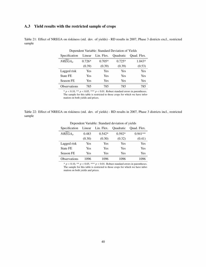
A.3 Yield results with the restricted sample of crops

Table 21: Effect of NREGA on riskiness (std. dev. of yields) - RD results in 2007, Phase 3 districts excl., restrictedsample

Dependent Variable: Standard Deviation of YieldsSpecification Linear Lin. Flex. Quadratic Quad. Flex.gNREGAit 0.726* 0.705* 0.725* 1.043*


Observations 785 785 785 785* p < 0.10, ** p < 0.05, *** p < 0.01. Robust standard errors in parentheses.The sample for this table is restricted to those crops for which we have infor-mation on both yields and prices.

Table 22: Effect of NREGA on riskiness (std. dev. of yields) - RD results in 2007, Phase 3 districts incl., restrictedsample

Dependent Variable: Standard deviation of yieldsSpecification Linear Lin. Flex. Quadratic Quad. Flex.gNREGAit 0.483 0.542* 0.592* 0.941**


Observations 1096 1096 1096 1096* p < 0.10, ** p < 0.05, *** p < 0.01. Robust standard errors in parentheses.The sample for this table is restricted to those crops for which we have infor-mation on both yields and prices.

40

A.4 A Measure of Mobility

Apart from the “implicit insurance” channel, the NREGA could affect individual decision making by relaxing other

constraints as well. For example, by relaxing credit constraints the Act could permit farmers to incur the fixed costs

associated with switching production away from crops they have been growing in the past, and into crops that they

perceive will provide them with the highest returns. If that is the case, we would observe greater mobility in crop

choice as a result of the program. In order to test whether or not this is really the case we develop a measure of crop

mobility and describe how to decompose it into movements that are risk-increasing and those that are risk-reducing.15

Consider an agent who enters a period with some assets, a and a “crop inheritance”, q. This crop inheritance should be

thought of as the crop which was being grown on his land in the previous period. At the beginning of this period, the

agent receives a preference shock, which provides a preference ordering over the crops. This preference shock should

be interpreted as a reduced form for information that the analyst does not have. For example, the agent might learn of

a new technology that he wants to implement, or learn that his parcel of land is more suited to growing certain kinds

of crops.

Once this preference shock is realized, the agent might want to switch away from his inherited crop, and towards some

other crop. Now, to make this switch, the agent must incur a fixed cost F. This can represent the cost of new seeds, of

equipment that needs to be purchased for the new crop, or simply of the time and effort required to acquire information

about how to tend for the new crop. If the agent’s asset levels are lower than F, he would need to borrow. If access

to credit is limited and borrowing constraints bind, then the agent may be forced to continue production of q. In such

a situation, if the introduction of the NREGA relaxes borrowing constraints, then we would expect to see increased

mobility across crops. Some of this increased mobility would be in the direction of increased risk-taking, and some of

it would just reflect the idiosyncratic preference shock. The natural question then is, is it possible to decompose the

overall mobility in crop choice into movement towards increased risk, and movement towards decreased risk?

To fix ideas, consider a district growing n crops. We arrange the crops in decreasing order of riskiness as measured

by the standard deviation of yields or revenues, so that crop 1 is the riskiest and crop n is the least risky. Let Y1 =

(a1, a2..., an) represent the land allocation vector in this district in year 1 and Y2 = (b1, b2..., bn) be the allocation in

year 2.

Define 4 = Y2 � Y1 to be the “switch vector”, which records all the shifts in land allocation across the years. |4| =Pn

i=1 |(ai � bi)| is one possible measure of the overall mobility in crop choice across the year. A larger value for |4|

indicates more ”churning” or movement within crops, and a smaller value indicates more persistence in land allocations15We would like to thank Debraj Ray for suggesting this conceptual framework.

41

among crops. From the definition, it follows that |4| 2 [0, 2].16 Now we develop a measure which decomposes |4| into

risk-increasing moves and risk-reducing moves.

What is a basic property would we want such a decomposition to satisfy? Consider an illustrative example where the

change in land distribution vector is given by

4 = (0.1, 0.4,�0.2,�0.3) (3)

Looking at this vector we can see that district reduced production of crops 3 and 4, and increased its production of

crops 1 and 2. Since we have arranged crops in order of decreasing risk, we would say that all the shifts that have

taken place in this district have been in the direction of greater risk.

More generally, if the 4 vector satisfies “single crossing at 0”, then our decomposition should be able to unambiguously

label the shifts as being risk-taking or risk-reducing. The ”single crossing” property can be satisfied in two ways. One

possibility is that the initial few entries of the vector are entirely positive, and the latter entries are all negative values.

This means there has been a move from the less risky crops to the more risky crops, and no move in the reverse

direction. An example of such a vector is the one depicted above in equation 3. In this case our decomposition

should assign all the moves as risky. Conversely, if the initial components of 4 are negative and the latter components

are positive, we should be able to say that all moves have been towards lower risk. An example of such a vector is

4 = (�0.1,�0.4, 0.2, 0.3).

Of course, the 4 vectors in the data do not satisfy this single crossing at zero property, and we therefore need to define

a measure of decomposition which can be used for general vectors, but which also satisfies the above criterion when 4

does indeed “cross” zero just once. We explain this measure using a simple example of a vector that does not satisfy

the single-crossing property. Let

4 = (�0.1, 0.3,�0.4, 0.2) (4)

In this example we are moving out of crops 1 and 3, and into crops 2 and 4. More generally say we are moving out

of crops i and k and into crops j and l. Take crop i which we are ”moving out” of and transfer the land lost into crops

j and l in a manner proportional to the final land allocated to the crops which are ”moving into”. Precisely, let Ti j

represent the transfer from crop i to crop j. Then in the above example

T12 =0.3

0.3 + 0.2(0.1)

T14 =0.2

0.3 + 0.2(0.1).

16Pni=1 |ai | �

Pni=1 |bi |

Pni=1 |(ai � bi)|

Pni=1 |ai | +

Pni=1 |bi |, and

Pni=1 |ai | =

Pni=1 |bi | = 1.

42

Similarly, for crop 3 we have

T32 =0.3

0.3 + 0.2(0.4)

T34 =0.2

0.3 + 0.2(0.4).

Then set all other transfers equal to 0. So T21 = T23 = T41 = T42 = 0.

Now since we have arranged crops in decreasing order of crop riskiness, we define a transfer Ti j to be risk-increasing

if i > j and risk-reducing if i < j. In our example, therefore, T12, T14 and T34 are risk-reducing moves, and T32 is a

risk-increasing move. Finally, define:

R+ =n

X

Ti j|i > jo

and

R� =n

X

Ti j|Ti ji < jo

R+ is a measure of the value of all risk taking moves, and R� is a measure of the value of all risk reducing moves. It is

then trivial to see that

R+ + R� =|4|2

We therefore have a valid decomposition. This decomposes all the movement in land allocation in the economy into

those moves that are in the direction of increased risk and those that are not. This is the third measure of risk and

mobility which we use to estimate the impact of the program.

In order to calculate the total changes and divide them into risk-taking and reducing, we rank crops in a particular

district-state-season combination based on the standard deviation of the revenues at retail prices over the period for

which we have this information. Thus a particular crop could be the riskiest in one district and have a completely

different ranking in another district. Having ranked crops in this manner, we can look at changes in the allocation of

total land across these crops and how that changes from one year to the next, in the manner described above.

Tables 23, 24 and 25 present the results for the endline for the total number of changes of crop land allocation from

2006 to 2007, and for how many of those changes are risk-increasing and how many are risk-reducing. In order to

perform this calculation we rank crops based on the standard deviation over time in the revenues generated from them.

The results show that there do not seem to be significant differences across districts that received the NREGA and those

that did not. Of course the calculations here and in the previous results are not necessarily capturing the same measure,

and so this is not in contradiction to the increase in the coefficient of variation results we presented earlier. However

it is interesting to see that (though insignificant) the coefficients are in line with our hypothesis - districts receiving

43

NREGA seem to be making fewer risk-reducing moves, more risk-increasing moves, and more moves overall.

One of the ways to reconcile the finding of higher risk in yields and revenues through higher variances in portfolios

with the fact that we do not find churning in the land allocation is the following: Many farmers do not necessarily

take on greater risk by choosing to cultivate a different crop entirely, but simply by substituting one low-risk variety

with another higher-risk higher-yield variety of the same crop (see Mobarak and Rosenzweig (2014)). Since our

dataset does not distinguish between the different varieties of crops, we might simply be under-equipped to answer

the question of whether the number of risk-increasing or risk-reducing moves has changed since the introduction of

this program. It is possible that crop changes occur within a crop but across varieties with greater frequency than they

occur across crops.

Table 23: Effect of NREGA on total land allocation changes - RD results in 2007, Phase 3 districts excludedDependent Variable: Total amount of land reallocated

Specification Linear Lin. Flex. Quadratic Quad. Flex.gNREGAit 0.062 0.020 0.066 0.116

(0.41) (0.42) (0.41) (0.56)

State FE Yes Yes Yes YesSeason FE Yes Yes Yes YesObservations 1044 1044 1044 1044

* p < 0.10, ** p < 0.05, *** p < 0.01. Robust standard errors in parentheses.

Table 24: Effect of NREGA on risk-reducing land reallocations - RD results in 2007, Phase 3 districts excludedDependent Variable: Total amount of land reallocated

in a risk-reducing fashionSpecification Linear Lin. Flex. Quadratic Quad. Flex.gNREGAit -0.355 -0.372 -0.353 -0.155

(0.26) (0.26) (0.26) (0.35)



44

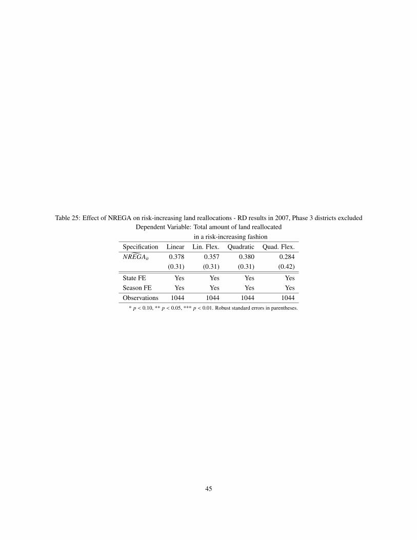
Table 25: Effect of NREGA on risk-increasing land reallocations - RD results in 2007, Phase 3 districts excludedDependent Variable: Total amount of land reallocated

in a risk-increasing fashionSpecification Linear Lin. Flex. Quadratic Quad. Flex.gNREGAit 0.378 0.357 0.380 0.284

(0.31) (0.31) (0.31) (0.42)



45

providing more than just employment? evidence from the ... · providing more than just employment?...

Documents