Providing a Healthier Start to Life: The Impact of

Conditional Cash Transfers on Infant Mortality�

Tania BarhamDepartment of Agriculture and Resource Economics

U.C. Berkeleyy

January 19, 2005

Abstract

In this paper, I evaluate the impact of Mexico�s conditional cash transfer program,

Progresa, on infant mortality. While studies on other aspects of Progresa make

use of a randomized treatment and control evaluation database performed in 506

communities, this database lacks su¢ cient sample size to measure the e¤ect on infant

mortality. Instead, I use vital statistics data to determine municipality-level, rural

infant mortality rates and create a panel dataset covering the period 1992-2001. I

take advantage of the phasing-in of the program over time both between and within

municipalities to identify the impact of the program. I �nd that Progresa led to

an 11 percent decline in rural infant mortality among households treated in Progresa

municipalities. Reductions are as high as 36 percent in those communities where,

prior to program interventions, the population all spoke some Spanish and had better

access to piped water.

�I would like to thank Elisabeth Sadoulet, Alain de Janvry, and Paul Gertler for their invaluable supportof this work. I am also grateful to Jean Lanjouw, Guido Imbens, and students and professors in the UCBerkeley development community whom have provided so many useful comments. In addition, I amthankful to all those in the Department of Health Economics at the Mexican National Institute of PublicHealth, Mexican Ministry of Health, IMSS-Oportunidades and Oportunidades who graciously providedme with the data and their institutional knowledge. Finally, this work was made possible by the �nancialsupport of the Institute of Business and Economic Research at UC Berkeley and UC MEXUS.

yPRELIMANARY DRAFT- please do not cite. Any comments are greatly welcome. Please directcorrespondence to tbarham@berkeley.edu.

1

1 Introduction

Every year more than 10 million children die from preventable diseases such as malnutri-

tion and intestinal infections in developing countries (World Bank, 2003). The majority

of these deaths take place during infancy, before the child reaches the age of one.1 Con-

sequently, �nding e¤ective policies to reduce mortality among infants is a key part of the

development agenda. This is evidenced by the selection of infant mortality as one of

the targets of the Millennium Development goals (World Bank, 2003). Conditional cash

transfer programs are a new type of social investment tool designed, amongst other goals,

to improve the health of children, but which may also lead to important reductions in

infant mortality. However, empirically establishing causality between the implementa-

tion of conditional cash transfers and infant mortality is di¢ cult because the death of an

infant is a relatively rare event. Thus, large sample sizes are a requirement for accurate

estimation. Even large household surveys commonly do not have a su¢ cient number of

observations to examine infant mortality. In 1997, Mexico implemented one of the �rst,

largest, and most innovative conditional income transfer programs, Progresa.2 Owing

to its extensiveness, Progresa provides an opportunity to test the causality of conditional

cash transfers on the infant mortality rate (IMR).3 In this paper, I use non-experimental

methods that exploit the phasing-in of Progresa over time throughout rural Mexico to

examine if this new policy tool reduced the rural IMR in Mexico.

Progresa di¤ers from typical income transfer programs since the cash transfers to ben-

e�ciary households are made conditional upon household members engaging in a set of

actions designed to improve their health, nutrition and education status. The aim of the

program is to build the human capital of young children and thereby break the intergen-

erational transmission of poverty. Previous research on Progresa has taken advantage

of a randomized treatment and control evaluation database to investigate if the program

improved various aspects of children�s health.4 This research has shown that the nutri-

tional status of children improved and the number of days a mother reported her child

1According to the World Bank�s World Development Indicators, the 2002 mortality rate for children(the probability that a child dies before reaching the age of �ve per 1000 live births) in low and middleincome countries was 88, while the infant mortality rate (the probability that a child dies before the ageof one per 1000 live births) was 60.

2Progresa stands for Programa de Educatión, Salud y Alimentación. This program is now known asOportunidades.

3The infant mortality rate is de�ned as the number of children in a given year who die before the ageof one per 1000 live births in the same year.

4The evaluation database is a panel of household surveys that contains information on the treatmentand control households both before and after the intervention.

2

ill decreased for treatment households as compared to those from similar families that

did do not receive the transfer (Behrman and Hoddinott, 2001; Gertler and Boyce, 2001;

Gertler, 2004). These �ndings indicate that there are some important nutritional ben-

e�ts of conditional cash transfers, but most other indicators of children�s health used in

these studies rely on parent�s recall and perceptions of good health which have potential

reporting biases. This paper therefore focuses on infant mortality, which is a broader and

more objective measure of children�s health.5

In addition, the sample size in the Progresa randomized treatment and control data-

base is too small to accurately estimate the impact of the program on infant mortality.

This paper resolves the sample size problem by constructing a panel data set of 2,399

municipalities6 from 1992 to 2001 and uses a non-experimental research design. The

treatment e¤ect of Progresa on rural infant mortality is identi�ed using the phasing-in

of the program over time in rural Mexico. This leads to a variation in the intensity

of treatment indicator � the percent of the rural population covered by the program �

both within and between municipalities. The econometric model employs municipality

and time �xed e¤ects, and includes variables associated with the program phase-in rule

to control for program timing bias. The analysis also explicitly controls for changes in

the supply of health care in rural areas. Additionally, the identi�cation strategy takes

advantage of the fact that Progresa was not provided in urban areas prior to 2000, and

uses the urban IMR to test whether unobservable municipal time-variant variables are

biasing the results. Using these techniques, I �nd that the program led to a reduction

of approximately 2 deaths per 1000 live births among program participants. From an

average IMR of 18, this is an 11 percent reduction. Reductions in infant mortality were

even higher in Progresa areas where, prior to the program, houses had better access to

piped water, fewer sewage systems, and in areas where the population spoke some Span-

ish.7 Furthermore, robustness checks show that the program had no spurious impact on

5 The IMR is commonly used as a primary indicator of children�s health, especially in developingcountries. This is partly due to inadequate information systems to gather data on child morbidity inmany countries, and because obtaining objective measures of children�s health that do not rely on parent�srecall or perceptions of good health is di¢ cult. In addition, infants are especially susceptible to manycommon diseases. Thus, their death rate serves as an indicator of the overall health of children in areasthat su¤er from high rates of preventable diseases (Lederman, 1990; Population Reference Bureau, 2004).

6 In the 2000 Census there were 2445 municipalities in Mexico with an average population of 40,000people and an average size of 800 squre kilometers. They are often compared to the size of a county inthe US.

7Mexico has a large indigenous population and there are areas where this population does not speakSpanish.

3

urban infant mortality, and also show that the impact is not the result of an endogenous

increase in the number of live births.

With the exception of Progresa, there is very little evidence at this time of the causal

impact of conditional or unconditional cash transfer programs on children�s health out-

comes or mortality in other developing countries. Results from the Colombian conditional

cash transfer program show that while the number of episodes of acute diarrhea decreased

among children under 6 years of age, there was no improvement in nutrition (Rawlings,

2004). In contrast, the conditional cash transfer program in Nicaragua led to a signi�cant

reduction in malnutrition (Maluccio & Flores, 2004). Studies on the e¤ect of increasing

the amount and coverage of the social pension program in South Africa for the elderly

black population found that income transfers also led to nutritional improvements among

girls (Du�o, 2003; Case, 2001). The present study therefore makes an important con-

tribution to the literature on health impacts of cash transfer programs by investigating a

di¤erent and important children�s health indicator, infant mortality. It is also the �rst

study to use government administrative data to investigate outcomes of conditional cash

transfer programs that could not have been studied otherwise.

The remainder of the paper is organized as follows. Section 2 describes the Progresa

program including the targeting mechanism and the phase-in rule. A description of the

data is provided in section 3. The identi�cation strategy, including an explanation of

the sources of variation in the treatment variable and the empirical model is presented in

section 4. Results are provided in section 5 and section 6 concludes.

2 The Rural Progresa Program

Adopted in 1997, Progresa aims to break the intergenerational transmission of poverty

by improving the human capital of poor children in Mexico. The program targets the

rural poor reaching nearly 2.5 million rural households by 2000. The Progresa model

is extremely popular throughout the Latin American region and has been adopted by

Argentina, Colombia, Honduras, Jamaica, and Nicaragua.

Progresa is unique in that it combines two traditional methods of poverty alleviation:

cash transfers and free provision of health and education services. These programs are

linked by conditioning the cash transfers on children attending school and family members

obtaining su¢ cient preventative health care. Therefore, the income transfer not only

relaxes the household budget constraint, but also provides an increase utilization of health

and education services. While the program was �rst introduced in rural areas, it expanded

4

into urban areas in 2000. This study focuses on the rural program.

The health component of Progresa was designed to address many recalcitrant health

issues in rural Mexico. For instance, the program targets infants, children, and pregnant

and lactating women in an e¤ort to ensure a healthier start to live. In addition, the

cash transfers are conditional on the household�s participation in four important health

activities:

1. growth monitoring from conception to age 5;

2. regular preventative health check-ups for all family members, including prenatal

care, well baby care and immunizations;

3. mother�s attendance at health, hygiene and nutrition education programs; and

4. children ages 0-2 and pregnant and lactating women taking nutritional supplements.

Adequate prenatal care, medical assistance at birth, immunizations and good breast-

feeding practices � all aspects of the Progresa program � are known to be important

for proper in-uterine growth of a child and for reducing the probability of infant death

(Murata et. al., 1992; Costello and Manandhar, 2000; World Bank, 2003). Thus, we

may expect the program to reduce infant mortality. In fact, research has shown that

programs in the US that target poor families and are similar to Progresa in terms of the

type of health interventions, but do not provide an income transfer, have led to reductions

in infant mortality (Currie and Gruber, 1996; Devaney et. al., 1990).

Since it was expected that health care utilization would rise as a result of the program,

Progresa coordinated with other government ministries responsible for health care delivery

to ensure an adequate supply and quality of health care in program areas. In addition,

the program used mobile clinics and foot doctors to reach many marginalized communities

that did not have access to permanent health clinics.

2.1 Targeting and Program Phase-in

Progresa used a two-stage process to identify eligible bene�ciary households in rural areas

(Skou�as et. al, 1999). In the �rst stage, rural localities8 were selected. Localities

8A locality is a cluster of inhabited houses that can vary in size from 1 dwelling to over a millionand has an average population size of 489. Localities are grouped into municipalities. The 2000 censusrecorded that there were 199,391 localities in 2,445 municipalities in Mexico. This leads to an average of80 localities in a municipality with the range from 1 to 1630. A municipality is approximately 100 times

5

with 2,500 inhabitants or less are denominated as rural.9 In order to meet the program�s

objectives, localities where chosen based on a number of attributes. Localities were �rst

ranked by a marginality index10 and only those with a high marginality11 were included

in the program. Next, localities were screened to ensure access to primary and sec-

ondary schools as well as to a permanent health care clinic.12 Finally, the program used

population density data and information on the proximity of localities to each other to

determine the geographic isolation of the locality. This information was used to identify

groups of localities where the maximum bene�t per household in extreme poverty would

be reached. As a result, any locality with less than 50 inhabitants or that was determined

to be geographically isolated was excluded from the program.

While the exact program phase-in rule is not clearly documented, the general criteria

are known (Skou�as et. al., 1999). For logistical and �nancial reasons, the program was

phased-in over time starting with 2,578 localities in 7 out of 32 states in 1997 (see Figure

1). In 1998, the program was greatly expanded, reaching almost 34,000 localities and

all but two states. In this year, the requirement that localities must have access to a

permanent health clinic was relaxed. In 1999, localities that were eligible but not yet

included and some localities which were previously excluded due to geographical isolation

were also incorporated into the program.

Once localities were selected, bene�ciary households in each community were identi�ed.

A census, called the Encaseh, was taken of all households in the program localities. This

census collected information on household income and characteristics that captured the

multidimensional nature of poverty. Using these data, a welfare index was established

and households were classi�ed as poor or non-poor. Only the poor became eligible for

bene�ts. Lastly, the list of potential bene�ciaries was presented to a community assembly

for approval. As a result, a di¤erent percent of the rural population is covered by the

larger than a locality with an average population of 40,000 as compared to 489 in 2000. The averagepopulation in rural areas of a municipality is 10,306, while the mean population of a rural locality is 125.

9Of the 199,391 localities in the 2000 census 196,350 were rural. The average number of people livingin a rural locality is 126.10This index is constructed using the principal components method. The variables that make up the

index include: literacy rate; percent of dwellings with running water, drainage, and electricity; averageoccupants per room; percent of dwellings with a dirt �oor; and percent of labor force working in theagriculture sector.11The marginality index was divided into quintiles based on the degree of marginality (for details, see

de la Vega, 1994). A grade of 5 indicates a high level of poverty and a grade of 1 a low level of poverty.Only those localities with a marginality grade of 4 or 5 were considered.12A locality was considered to have access to a health care clinic if the clinic was either in the locality

or in a neighboring locality at most 15 kilometers away (Skou�as et. al., 1999).

6

program in each locality. Recerti�cation of eligibility began in 2000.

2.2 The Randomized Experiment

A prominent feature of Progresa is the randomization of 506 program localities in seven

states into treatment and control groups. Eligible households in treatment villages re-

ceived bene�ts immediately, while eligible household in control villages became part of

the program about 2 years later. A baseline survey was performed in October 1997 and

six follow-up surveys were taken at approximately 6 month intervals. The design was

created in order to ensure rigorous evaluation of the program impacts. The delay in

the implementation of the program in control villages was justi�ed since the government

lacked su¢ cient funds to provide the program nationally from the outset. While many

studies on Progresa take advantage of these data, there are only two deaths of children

under age one in the control areas in the post-intervention period. For this reason, I use

vital statistics data and a di¤erent identi�cation strategy to study the program impacts

on IMR as explained in the following sections.

3 The Data

I constructed infant mortality rates using 1992-2001 vital statistics data. The mortality

data are from a nation-wide database containing information on every registered death in

Mexico and were provided by the Mexican Ministry of Public Health. While these data

are available at the municipality level, they do distinguish whether the death occurred in a

rural or urban locality within that municipality. The live birth data are publicly available

for every municipality in Mexico from the Mexican Statistical Agency, INEGI, except for

the state of Oaxaca in the year 2000.13 These data are provided annually by municipality

and size of the locality where the mother who gave birth resided. The rural and urban

infant mortality data are constructed by linking these two databases by municipality.14

The intensity of treatment indicator is the percent of rural households in a municipality

13While the urban and rural breakdown of the number of live births is missing for Oaxaca, the totalnumber of births is available from INEGI. To �ll in the missing values for the number of rural births in2000, I calculated the average of the ratio of rural to total birth for 1999 and 2001 in Oaxaca. I multiplythis ratio by the total number of births in 2000. I used a similar process to determine the number ofurban births.14Values for municipal rural infant mortality rates greater than 240 were set to missing. These values

were removed from the analysis because they are outliers. Removal of these values a¤ected a total of 58observations or less than 0.3 percent of the data.

7

receiving Progresa bene�ts. It is determined using Progresa administrative data and

INEGI census data. Progresa provided administrative data on the number of households

registered for the program in December of each year. This information is available for

each locality from the inception of the program in 1997 to 2001 (Figure 1). However,

I aggregate these data to the municipality level since the infant mortality rate is only

available at this level. Using INEGI census data on the number of rural and urban

households in a municipality for 1990, 1995 and 2000, I linearly interpolate the number of

households for each year between 1992 and 2001. Thus, the percent of rural households

receiving program bene�ts is simply the ratio of the number of bene�ciary households to

the total number of households in rural areas of a municipality.15

A variety of municipality characteristics are used as control variables in the analysis.

The marginality index is publicly available at the locality and municipality levels on the

CONAPO website for 1990, 1995 and 2000. Health supply data are not publicly available;

I collected them from the Ministry of Health and IMSS-Oportunidades at the locality level.

Data on other municipality characteristics were obtained from the INEGI 1995 Conteo16

and 2000 Census and are also at the locality level. Here again, this locality data is

aggregated to the municipality level. Lastly, the INEGI 1990 Census is used to provide

information on some locality characteristics.

Using these data, a municipality-level, panel dataset was constructed from 1992-2001.

However, municipality boundaries were rede�ned during this time period. In order to

make a consistent panel of municipalities from 1992-2001, municipalities which were split

in a particular year are amalgamated. This results in a balanced panel of 2,399 munici-

palities.

4 Identi�cation Strategy

4.1 Sources of Variation

My objective is to estimate the treatment e¤ect of Progresa on rural infant mortality.

Ideally, I would compare the IMR in treated rural localities with the counterfactual �

the IMR had Progresa not been available in the locality. Since the counterfactual is

never observed, I would take advantage of the phasing-in of the program over time and

use rural localities yet to be treated as the comparison group. Since infant mortality15Approximately 2 percent of all positive values of the treatment variable are greater than one. These

values are set to missing.16The Conteo is a shorter version of the Census.

8

is not available at the locality level, I instead investigate the impact of the program on

municipality-level, rural IMR. Similar to localities, new municipalities came onto the

program over time between 1997 and 2001 (see Figure 2) leading to variation in the

intensity of treatment across municipalities over time. Therefore, municipalities yet to

be treated can be used as comparison municipalities. The identifying assumption in this

case is that the changes in infant mortality observed in the comparison group are the same

as in the treatment group had they not received the program. Although it is not possible

to test this assumption, I can test that the pre-intervention trends in infant mortality are

the same between municipalities that joined the program in di¤erent years. If the trends

are the same in the pre-intervention period, they are likely to have been the same in the

post-intervention period in the absence of the program.

I test that the pre-intervention trends in rural IMR, IMRr; between municipalities

that joined the program in di¤erent years are the similar. Two sets of dummy variables

are used ENTERk and Y EARj; where k=1998-2001 and j=1991-1996. ENTERk takes

on the value 1 if the �rst program locality of municipality m was phased-in during year

k; and is zero otherwise. Y EARj are year dummy variables for 1991-1996 (years prior

to the program introduction). Using data prior to 1997, the equation used to test the

di¤erence in trends is:

IMRrmt = �0 +Pj�jY EARjt +

Pj

Pk

�jkY EARjt � ENTERkm + umt (1)

If the ��s are not signi�cantly di¤erent from zero, then the pre-intervention trends do

not statistically di¤er between municipalities entering the program in subsequent years.

Results are reported in Table 1. With the exception of the group of municipalities that

joined the program in 2001 and those municipalies that have no Progresa, the results

show that the pre-intervention trends in the rural IMR are not signi�cantly di¤erent from

municipalities that entered the program in 1997. Municipalities that joined the program in

2001 and those that do not have Progresa will therefore not be included in the comparison

group.

Not all Progresa localities within a municipality were phased-in to the program during

the same year. As a result, the program intensity also varies over time within a munic-

ipality. For example, Table 2 shows that there were 2,424 Progresa localities in 1997.

In 1998, the number of Progresa localities in those same municipalities almost doubled

to 4,705. This variation in program intensity within a municipality over time is another

source of variation used to identify the program impact.

9

Results may be biased if Progresa localities that were phased-in during di¤erent years

within a municipality are not similar. One way to reduce this bias is to control for the

program phase-in rule. Since localities that joined the program in 1997 had better access

to permanent health care clinics than those that joined the program later, I control for

changes in the supply of health care in rural municipalities, as well as the percent of

Progresa localities with access to a permanent health care clinic. Furthermore, localities

with lower population densities were phased-in during 1999. While I do no know the

density of rural areas of the municipality I can control for the density as a whole for the

municipality.

Ideally, I would also test that the pre-intervention trends in rural IMR are the same

between localities that were phased-in to the program in the various years. Since these

data do not exist, instead I examine if locality characteristics in the pre-program period

(1995 or 1990), and the change in locality characteristics between 2000 and the pre-

program period are the same across phase groups. To the extent that the level and change

in locality characteristics are correlated with the trends in rural IMR, their similarity across

phase groups is an indication that the trends in rural IMR are also likely to have been

similar in these localities.

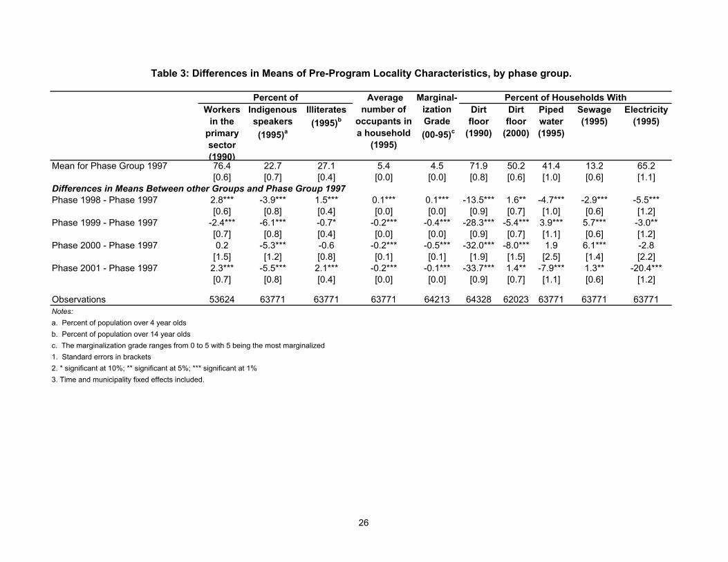
Table 3 presents the di¤erence in locality characteristics across phase groups in the

pre-intervention period. The means for localities that were incorporated into the program

in 1997 (phase group 1997) are reported in the �rst row. The di¤erence in the locality

characteristics between phase group 1997 and each of the other phase groups are reported

in subsequent rows. These di¤erences in these means are almost all signi�cant. With the

exception of the percent of population with a dirt �oor in 1990 and localities that where

brought into the program in 2001, means are within 10 percentage points. While these

di¤erences are arguably small, there is concern that they could bias the results. The trends

in the infant mortality rate between phase groups may be more likely to be determined by

the changes in locality characteristics rather than their level. Table 4 presents the change

in mean locality characteristics between 2000 and 1995 for localities that were phased-in

during 1997 in the �rst row. The subsequent row show how this change di¤ered between

the 1997 phase-in group and those localities the joined the program in later years. Now

the majority of the di¤erences in the changes between phase group 1997 and each of the

other groups are not signi�cant (see Table 4). In order to account for these di¤erences

in the observables, these variables are included as covariates. If the �ndings do not vary

when these variables are included, it is hoped that similar changes in the unobservables

10

would also not bias the results. However, locality observables must be aggregated to the

municipality level in order to be included in the analysis.

In addition, inclusion of municipality �xed e¤ects controls for biases due to di¤er-

ences in time-invariant variables across municipalities arising from non-random program

placement (Rosenzweig and Wolpin, 1986). The estimate of the treatment e¤ect will be

unbiased if there are no unobserved time-varying municipality characteristics or trends

that are correlated with the intensity of treatment variable. If this is the case, the ur-

ban infant mortality rate should not be a¤ected since the program targeted rural areas.

However, if there were important omitted municipality time trends correlated with the

treatment variable, I would expect to �nd an impact of the program on urban infant mor-

tality due to the unobservables. Therefore, in the results section I also present results

for urban IMR to test if there are municipality time trends that could be biasing the

results. Lastly, I will also present a validity check where I include a time trend for each

municipality to account for further variation over time between municipalities resulting

from to these unobservables.

4.2 Graphical Analysis

Due to the variation in the intensity of treatment both between and within municipalities

over time, it is di¢ cult to show the treatment e¤ect graphically. However, graphs can

provide suggestive evidence. In Figures 3-5, trends in average municipality rural IMR

are provided for three groups of municipalities, based on the year the program was �rst

o¤ered in the municipality. Only municipalities that entered the program in 1997, 1998

and 1999 are shown on the graphs. Municipalities that entered in 2000 are not displayed

since there are just 12 observations. Those that joined in 2001 are also excluded since the

pre-intervention trend for this group is statistically di¤erent from the other municipalities.

Trends in urban IMR over the same time period are presented in Figure 6. Finally, since

program intensity varies between municipalities, trends in rural IMR are also presented

only for municipalities that had an average program intensity of 30 percent or more over

the program period (Figure 7).

If Progresa is successful, there should notice a break in the trend in rural IMR soon after

the program entered the municipality. However, since the program intensity increased

over time within a municipality, these breaks may not be visible in the �rst year of the

program. Mean municipality program intensity by year for each of the three groups are

presented in Table 5. The �rst group of municipalities began to receive the program in

11

1997. Only 24 percent of rural households in these municipalities were covered by the

program in that year. In 1998, the program was greatly expanded covering 55 percent

of rural households in these same municipalities. Thus, there may be a larger impact of

the program in 1998 rather than 1997 for this group. Figure 3 demonstrates that this is

indeed the case for the municipalities that entered the program in 1997. The break in the

trends for the two other groups occur the year the program entered the municipalities. I

verify that these breaks are not due to general trends in the municipalities by presenting

a similar graph for urban IMR. As expected, there are no breaks in the trend in urban

IMR the year the program entered the municipalities.

4.3 Empirical Model

I develop the empirical model by �rst considering a cohort of infants that dies in year t, in

municipalitym. Whether an infant dies, (D = 1), during that year depends on (i) whether

the infant was born in a household registered for Progresa bene�ts or not that year, and

if the infant�s mother was registered for the program during her pregnancy17, Ht; Ht�1;

Ht�2; (ii) mother and household characteristics, I, and; (iii) municipality characteristics

such as the supply of health care or the quality of the environment (both time-varying and

time-invariant), X. Time �xed e¤ects are included to control for time trends. Assuming

a linear relationship,

Pr(Dimt = 1) = �t +Pj�jH

t�jimt +

Pg�gIimtg +

Pp�pXmtp + "imt; (2)

where imt indexes infant i born alive in municipality m in year t, and j = 0 � 2. Year

�xed e¤ects are represented by �t; and "imt is the error term, which is assumed to have a

zero mean and be orthogonal to the independent variables.

There are a number of variables in equation 2 that are not observed in the data. The

indicator variable Himt (if child imt is from a program household or not) does not exist

at the individual level in the dataset, however, the probability of treatment at the munic-

ipality level does. This probability is the percent of live births to bene�ciary households

in municipality m in year t, and is the same for all infants in the municipality. Thus, I

use this value in lieu of the individual Himt. Also, mother and household characteristics

of the infant are not available in the Mexican vital statistics.17Although an infant dies in year t, it may have been born in year t-1, and been in the womb in year

t-2. Therefore, two program lags are included in order to cover the life of the child from conception toage one.

12

Given the lack of individual-level data and because mortality is identi�ed at the mu-

nicipality level, equation 2 is aggregated to the rural municipality level as follows:

Xi2Im

Dimt = Nmt�t +Pj�jPB

t�jmt +Nmt

Pp�pXmtp +

Xi2I"imt; (3)

where Nmt is the population of the infants (<1 year old) born alive in the rural areas of

municipality m in year t and Im is the set of infants born alive in municipality m. The

dependent variable is now the number of deaths among infants born alive in a municipality

in a given year, and the treatment variable, PBmt;is the number of live births in munic-

ipality m in year t to Progresa households in year t � j. To make comparisons across

municipalities, equation 3 is normalized by the number of live births in each municipality.

At the municipality level, the equation is written as follows:

1

Nmt

Xi2IDimt = �t +

Pj�jPBt�jmt

Nmt+Pp�pXmtp +

Xi2I

"imtNmt

(4)

The database provides information on the number of program households not the

number of births to Progresa households, PB. Assuming that the fertility rate remains

constant over the period of the program (1997 - 2001), I rede�ne PBt�jmtNmt

to be the ratio of

the number of bene�ciary households over the total number of households in rural areas of

the municipality in a given year. This is the intensity of treatment or program intensity

variable, referred to as Intensity. Municipality �xed e¤ects are also added to equation

4 to control for time-invariant municipality characteristics that could be correlated with

both infant mortality and program intensity due to program placement bias.

The estimation equation is

IMRrmt = �t + �m +Pj�jIntensity

r;t�jmt +

Pp�pX

rmtp + umt; (5)

where the r superscript is added to emphasize that these data are for rural areas of the

municipality. The dependent variable is now labeled IMRr since it is a measure of

the rural infant mortality rate. Heteroskedasticity and serial correlation mayb both be

present in the error term. Thus, the regressions are weighted by the number of rural

households18 and robust standard errors that are corrected for serial correlation19 are18While the equations suggest weighting by the number of live births, this variable su¤ers from under-

reporting in Mexico so the number of rural households is used because it provides a more consistentweight.19The correction for serial correlation is made by clustering the standard errors at the municipality level.

13

used. The estimate of the treatment e¤ect of Progresa on the treated is measured by the

��s, while the average treatment e¤ect can be calculated by multiplying the impact on the

treated by the average of the Intensity.

5 Results

5.1 General Impact of the Program

I start by estimating the treatment e¤ect of Progresa on the rural IMR. Columns 1 through

5 of Table 6 presents di¤erent speci�cations for estimating this impact. The adjusted R2

is the same for each of the speci�cations, and the lag of the treatment variable, program

intensity; consistently provides the only signi�cant result. Therefore, the speci�cation

depicted in column 5, which includes only the lag of program intensity as an explanatory

variable, is the primary estimation of the treatment e¤ect. This result shows that among

the treated the probability of an infant dying is reduced by almost 2 deaths per 1000 live

births on an average of 18 deaths, or 11 percent. At the municipality level, the percent

of rural households covered by the program reached an average of 47 percent. Therefore,

the average treatment e¤ect is a 5 percent reduction in the rural IMR.

5.2 Spillover E¤ects

Reduction in infant mortality among the treated may be overestimated due to the inabil-

ity to exclude non-eligibles (non-poor in a locality) from bene�ting from the improved

health supply or due to program spillover e¤ects. While cash transfers are only provided

to bene�ciaries, improvements in the health supply associated with the program could

potentially lead to mortality reduction in the non-eligible group. Furthermore, program

bene�ciaries may inform those not in the program of the health gains they experienced

from increased health care utilization or share their knowledge from the health education

session. These health spillover e¤ects could also generate lower infant mortality rates

among the untreated.

Bobonis and Finan (2002) study health spillover e¤ects and �nd no indication of such

e¤ects on the incidence of illness or on self-reported health indicators for children. This

provides partial evidence that spillover e¤ects may not be a concern. However, it may

be that women�s health behaviors during pregnancy and their child�s infancy are not

related to behaviors that a¤ected the children�s health outcomes mentioned above. While

this question can be investigated further using the randomized treatment and control

14

evaluation database, the average treatment a¤ect reported in this paper provides a lower

bound on the impact of the program on the treated.

5.2.1 Validity Checks

Although the model controls for time-invariant unobserved municipal heterogeneity, it

cannot control for unobserved time-varying municipality factors that may be correlated

with the treatment variable and infant mortality. I take advantage of the fact that

Progresa mainly operated in rural localities before 2001 and test whether the program

had a signi�cant impact on urban IMR.20 If there are indeed municipal-level omitted

variables, program intensity might also impact urban IMR due to these unobservables.

Table 6, column 6 show that the program had no signi�cant impact on urban IMR, thereby

providing some evidence that unobservables are not biasing the results.

A further concern is that during program implementation there was an expansion of

health care in rural communities. To control for possible biases, information on per capita

health care infrastructure and personnel are included in the regression equation. Although

many of these regressors are likely to be endogenous, if their inclusion does not in�uence

the coe¢ cient on the lag of the program intensity, we gain some con�dence that health

care supply is not correlated with the phasing-in of the program. The results in columns

1 to 3 of Table 7 demonstrate that the program impact remains unchanged.

During the �rst three years of the program, two criteria for choosing localities were

relaxed. After 1997, the condition that bene�ciaries had to have access to permanent

health clinic no longer applied as mobile clinics and foot doctors also provided health

care in many areas. Also, in 1999, localities that had a lower population density and

were isolated from other Progresa localities were incorporated in the program. I include

a variable de�ned as the percent of rural Progresa localities with access to permanent

health clinic in a given year to take into account the �rst change in the phase-in rule.

The addition of this control has almost no e¤ect on the estimate of the impact and is not

signi�cantly di¤erent from zero (Table 7 column 4). Additionally, I control for the density

of the municipality and the inclusion of this variable also does not change the estimate of

the impact Table 7 column 5).

I also control for all other observable time-varying municipality characteristics and

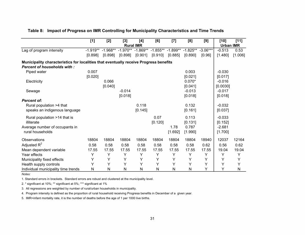
individual municipality time trends (see Table 8). The municipality characteristics are

20There are a some semi-urban localities that joined the program before 2000. The program did expandto urban localities in 2000 but this should not a¤ect our analysis.

15

generated from the locality census data and are the municipality means made by aggre-

gating data for localities that received Progresa bene�ts before 2001.21 The results do not

di¤er if the municipality characteristics for the rural areas of the municipalities is used

instead. Columns 1-8 clearly show that adding the available covariates does not e¤ect

the estimate of the impact. However, once a time trend is added for each municipality

to account for the trends in unobservables, the impact of the program on infant mortality

is higher. Progresa leads to a reduction of approximately 3 deaths per 1000 live births,

or 17 percent among the treated. This estimate is still inside the 95 percent con�dence

interval for the impact of the program with the individual time trends in column 5 of Table

7. However, the result suggests that omitted other time-varying municipal characteristics

may result in an under-estimate of the e¤ect of Progresa on infant mortality.

Finally, as discussed in section 4.1, the means and changes in means of locality char-

acteristics across phase-in groups were arguably small but signi�cantly di¤erent. Using

data on 1995 locality characteristics, I estimate the municipality mean by aggregating the

data only for localities that received Progresa for that particular year. So, as localities are

phased-in, the municipality mean will change to re�ect the di¤erence in pre-intervention

characteristics of the phase-in groups.22 Results are presented in Table 9 and demonstrate

that the point estimate of the treatment e¤ect varies from -1.6 to -2.6. However, none

of these values are signi�cantly di¤erent from the comparable program impact of -1.86 in

column 5 of Table 7.

5.3 Under-reporting of Births and Death

Under-reporting of both births and deaths is common in rural Mexico. The fact that the

urban municipality IMR is higher than the rural municipality IMR is partly a re�ection

of this phenomenon. As long as the under-reporting does not change in a manner that is

correlated with the lag of program intensity the estimates will be unbiased. However,

one might be concerned that mothers in program areas may be more likely to register

their child�s birth in hopes of receiving a cash transfer in the future. Or, more babies

may be born alive due to increased prenatal care utilization or improved mother�s health.

Thus, it is possible that the program impact is a result of an increase in the number of

registered live births rather than a reduction in mortality. To investigate if this is the

case, the impact of Progresa on the number of registered lives births per 1000 population

21At present, the locality data is only available for 1995 and 2000. Therefore, I linearly interpolatebetween these points to generate data for the missing years.22The municipality mean is set to zero in the time period before Progresa is available in a municipalitiy.

16

in a municipality is also examined. Results in Table 10 demonstrate that the treatment

variable, the lag of program intensity, had no impact on the number of live births per 1000

population. Thus, the estimate of the program impact is not the result of an endogenous

increase in the number of births23.

5.4 Heterogeneity of the Treatment E¤ect

Data from 1995 is used to examine if the program impact varies by pre-intervention char-

acteristics of Progresa areas within the municipalities.24 Findings from Table 11 highlight

that the program was more successful at reducing infant mortality in municipalities where

Progresa areas had better access to piped water, less access to sewage systems, and where

all the population spoke some Spanish. The treatment e¤ect does not vary due to di¤er-

ences in the percent of households with electricity25 or the percent of the population 15

years of age or older who are literate.

In particular, program impacts are higher in municipalities where at least 75 percent

of households in Progresa localities had access to piped water prior to the intervention.

Approximately a third of the Progresa municipalities fall into this group. The treated in

these municipalities experienced a reduction in infant mortality of approximately 5 deaths

per 1000 live births, while those in areas with less access to piped water only experienced

a reduction of 1.7 deaths. Given that the mean rural IMR over the sample period for the

group of municipalities with better access is 19 as compared to 17 in areas with less access,

this represents a decline in infant mortality of 28 and 10 percent respectively. The average

percent of bene�ciary rural households in municipalities in 1999 for these same groupings

is 40 as compared to 46. Therefore, the average treatment e¤ect of the program resulted

in a 4 percent reduction in rural IMR in those municipalities where access to piped water

is lower and a 12 percent decline in those municipalities with better access to piped water

1995.

The program also led to a much greater reduction in rural IMR in Progresa localities

where the population over four years of age all spoke some Spanish. This is the case

for 57 percent of the municipalities in the estimation sample. In particular, the rural

IMR for the treated declined by 6 deaths per 1000 live births, on an average rural IMR

of 17, or 33 percent. The average intensity of treatment in these municipalities reached

23Sko�as, 2001 reports a similar result.24Since the 1995 Conteo data is available at the locality level, it is possible to calculate the characteristics

of just the localities that eventually receive Progresa in a municipality.25Though this is signi�cant at the 10.5 percent level.

17

35 percent, so for these municipalities as a whole the infant mortality rate declined by 13

percent. In contrast, the rural infant mortality rate declined by 2 deaths per 1000 live

births in areas where some of the population in Progresa areas only spoke an indigenous

language. The mean rural IMR was 18 and the program intensity reached 53 percent in

these areas. Therefore the rural IMR fell by 11 percent among the treated and 6 percent

on average in these municipalities.

Lastly, the reductions in rural IMR mainly took place in the three quarters of the

municipalities where less than 30 percent of the households in Progresa localities had

some type of sewage system prior to program implementation. The decline in infant

mortality among the treated in these areas is similar to the main impact of the program

at 2 deaths per 1000 live births, or 11 percent.26 The treated in those municipalities with

better access to sewage experienced almost no decline in their infant mortality as a result

of the program. However, the average rural IMR was also lower in these areas prior to the

program at 17 as compared to 19.5 in areas with less access to sewage. This may seem

contradictory to the results from piped water, but less than 35 percent of the municipalities

had Progresa areas with both good access to piped water and sewage systems.

6 Conclusions

The conditional cash transfer program, Progresa, led to a signi�cant decline in infant

mortality in rural Mexico. Findings suggest that the program resulted in an 11 percent

reduction of the infant mortality rate among the treated. While I cannot test if there are

spillover e¤ects using the present dataset, their possible presence may lead to an over-

estimation of the impact. The average treatment e¤ect, which is a 5 percent reduction

in the rural infant mortality rate in municipalities where some of the population received

Progresa, is on the other hand a lower bound on the estimate of the impact on the treated.

Given that on average the rural IMR fell by less than 1 percent each year between 1992

and 1996, these are large declines in infant mortality.

Program e¤ects were even greater in areas where, prior to the program, Progresa

localities had better access to piped water, and a population that spoke some Spanish. In

particular, infant mortality declined by 28 and 33 percent among the treated in Progresa

areas that had more piped water and not only indigenous language speakers respectively.

26Approximately 40 percent of the observations fall into the group with better electricity access. Themean IMR for this group is 19 as compared 17 in areas with less access, and the intensity of treatment is40 percent in areas with more access as compared to 46.

18

The declines in infant mortality also mainly occurred in Progresa areas where fewer houses

had a sewage disposal system prior to the program. The municipalities that had a

relatively high level of sewage disposal, experienced little reduction in their mortality rate,

though the mortality rate was lower in these area before the program. Unfortunately, it

is somewhat di¢ cult to interpret these results since these variables could be proxies for

a number of di¤erent attributes. It is often argued that piped water is correlated with

clean water; if this is the case, these �ndings highlight that there is an association between

having safe drinking water prior to the program and more substantial reductions in the

rural IMR from conditional cash transfers in Mexico. Also, if the presence of a sewage

system is a proxy for a sanitary environment, larger reductions in rural IMR are also

associated with areas that were less sanitary prior to the program. This may be a result

of the health education component of Progresa. However, these are just hypotheses

and these data cannot provide further evidence. They would be interesting questions

to examine further using the nutrition information from the randomized treatment and

control database.

I presented evidence on the internal validity of these results. I showed that the

program did not lead to a reduction in the urban IMR which might have been the case

if the phasing-in of the program over time was correlated with other municipality trends.

I also controlled for the change in the supply of free health care in rural areas. This

is important since Progresa worked closely with other ministries to ensure an adequate

supply of health care. In addition, I provided evidence that the reduction in infant

mortality is not the result of an endogenous increase in the number of live births.

It is also of interest to policy makers to understand the mechanisms that led to this

reduction in infant mortality in Mexico. Extensions of this work will examine this question

by taking advantage of the randomized treatment and control database to explore the kinds

of health behavior changes that occurred as a result of Progresa. For example, among

other factors I will explore: if treated babies weighted more at birth than non-treated

babies; if treated mothers received more prenatal care, were more likely to have their

delivery attended by a medical attendant, or had better knowledge of how to make oral

rehydration salts; and, if treated families were more likely to make home improvements

leading to a more sanitary environment.

19

References

Alderman, H., 1986, The E¤ects of Income and Food Price Changes on the Acquisition of

Food by Low-Income Households, Washington, D.C., International Food Policy Research

Institute.

Alderman, H., 1993, �New Research on Poverty and Malnutrition: What are the Impli-

cations for Research and Policy?� in M. Lipton and J. Van der Gaag eds., Including the

Poor, Washington, D.C, The World Bank.

Attanasio, O. and R., Victor, 2000, �Consumption Smoothing in Island Economies: Can

Public Insurance Reduce Welfare?�European Economic Review, 44(7), 1225-58.

Behrman, J.R. and J Hoddinott, 2001, Program Evaluation with Unobserved Heterogeneity

and Selective Implementation: The Mexican Progresa Impact on Child Nutrition, Penn

Institute of Economic Research Working Papers no. 35.

Behrman, J.R., and A.B. Deolalikar, 1987, �Will Developing County Nutrition Improve

with Income? A Case Study for Rural South India,�Journal of Political Economy, 95(3),

108-138.

Bobonis, G and F. Finan, 2002, Do transfers to the Poor Increase the Schooling of the

Nonpoor? The Case of Mexico�s Progresa, mimeo, University of California at Berkeley.

Case, A., October 2001, Does Money Protect Health Status? Evidence from South African

Pensions, NBER working paper w8495.

Case, A., D. Lubotsky, and C. Paxson, June 2001, Economic Status and Health in Child-

hood: The Origins of the Gradient, NBER working paper w8344.

Chay K., M. Greenstone, July 2001, The Impact of Air Pollution on Infant Mortality:

Evidence From Geographic Variation in Pollution Shocks Induced by a Recession, mimeo,

University of California at Berkeley.

Conapo, 2001, La Poblacion de Mexico en el Nuevo Siglo.

Cook, C.A., K.L. Selig, B.J. Wedge, and E.A. Gohn-Baube, 1999, �Access to Barriers and

the Use of Prenatal Care by Low-Income, Inner-City Women,�Social Work, 44(2), 129-39.

Costello, A. and D. Manadhar eds., 2000, Improving Newborn Infant Health in Developing

Countries, Imperial College Press, London.

20

Currie, J. 1994, �The Welfare and the Well-Being of Children: The Relative E¤ectiveness

of Cash and In-Kind Transfers,�Tax Policy and the Economy, 8, 1-43.

Currie, J. and J. Gruber, 1996, �Saving Babies: The E¢ cacy and Cost of Recent Changes

in the Medicaid Eligibility of Pregnant Women�, The Journal of Political Economy, 104(6),

1263-1296.

Costello, A. and D. Manadhar eds, 2000, Improving Newborn Infant Health in Developing

Countries, Imperial College Press, London.

De la Vega, S., 1994, Construccion de un Indice de Marginacion. Masters thesis in Statis-

tics and Operations Research, UNAM, Mexico City, Mexico.

Devany, B., L. Bilheimer, J. Shore, 1990, The Savings in Medicaid Costs for Newborns

and Their Mothers from Prenatal Participation in the WIC Program, Mathematic Policy

Research Inc., Washington, D.C.

Du�o, E, 2003, �Grandmothers and Granddaughters: Old-Age Pensions and Intra-

household Allocation in South Africa�, The World Bank Economic Review ; 17(1): 1-25.

Gertler, P., and S. Boyce 2001, An Experiment in Incentive Based Welfare: The Impact

of Mexico�s Progresa on Health, mimeo, University of California at Berkeley.

Gertler, P., 2004, �Do Conditional Cash Transfers Improve Child Health? Evidence from

PROGRESA�s Control Randomized Experiment,� American Economic Review, 94(2),

336-341.

Heckman J. and V.J. Holtz, 1989, �Choosing Among Alternatives Non-Experimental

Methods for Estimating the Impact of Social Programs: The Case of Manpower Training�,

Journal of the American Statistical Association, 84(408), 862-72.

Lederman R.P.,1990, �Infant Morality and Prenatal Care,� in J.N. Natapo¤ and R.R.

Wieczorek eds.,Maternal-Child Health Policy: A Nursing Perspective, Springer Publishing

Company, New York.

Legovini, A. and F. Regalia, 2001, Targeted Human Development Programs: Investing in

the Next Generation, Inter American Development Bank Sustainable Development De-

partment Best Practices Series.

21

Maluccio, J. and R. Flores, July 2004, Impact Evaluation of a Conditional Cash Transfer

Program: The Nicaraguan Red De Protección Social, FCND Discussion Paper No. 184,

Washington, D.C., IFPRI.

Meyer D., 1995, �Natural and Quasi-Experiments in Economics�, Journal of Business &

Economics Statistics, 151-161.

Murata, P.J, E.A. McGlynn, A.L. Siu, R.H.Brook, 1992, Prenatal Care: A Literature

Review an d Quality Assessment Criteria, Rand, Santa Monica, CA. USA

Oportunidades, 2003, Informacion General, http://www.progresa.gob.mx/informacion_general/15072003

/historico%20de%20Cobertura.htm, accessed on August 5, 2003.

Population Reference Bureau, 2004, http://www.prb.org/Content/NavigationMenu/PRB/Educators

/Human_Population/Health2/World_Health1.htm, accessed on Oct 30th, 2004.

Rawling, L.. and G. Rubio, August 2003, Evaluating the Impact of Conditional Cash

Transfer Programs: Lessons from Latin America, World Bank Policy Research Working

Paper 3119.

Rosenzweig, M. and K. Wolpin, 1986, �Evaluating the E¤ects of Optimally Distributed

Public Programs: Child Health and Family Planning Interventions,�The American Eco-

nomic Review, 76(3), 470-482.

Schultz, P., 2001, School Subsidies for the Poor: Evaluating the Mexican Progresa Poverty

Program, Yale Economic Growth Center Discussion Paper: no. 834.

Skou�as, E., B. Davis, S. Vega, Dec. 1999, Targeting the Poor in Mexico: An Evaluation of

the Selection of Households into OPORTUNIDADES, International Food Policy Research

Institute, Washington, D.C., USA

Skou�as, 2001, Progresa and its Impact on the Human Capital and Welfare of Households

in Rural Mexico: A Synthesis of the Results of an Evaluation by IFPRI, Washington D.C.,

IFPRI working paper.

Skou�as, E., and S. Parker, 2001, �Conditional Cash Transfers and Their Impact on Child

Work and Schooling: Evidence from the PROGRESA Program in Mexico,�Journal of the

Latin American and Caribbean Economic Association, 2(1), 45-86.

22

Strauss, J., and D. Thomas, 1997, �Health and Wages: Evidence on Men and Women in

Urban Brazil,�Journal of Econometrics, 77(1), 159-185.

The World Bank, 2003, The Millennium Development Goals, downloaded from website:

http://www.developmentgoals.org/Child_Mortality.htm, Oct. 21.2003

23

Year Municipalities that entered in 1997

No Progresa 1998 1999 2000 2001Mean IMR 1990 = 21.17

1991 -3.704 5.813 0.99 0.462 17.876 3.793[0.903] [6.765] [0.999] [1.349] [22.539] [2.534]

1992 -3.758 -3.436 -1.809* -1.065 16.823 2.415[0.863] [4.660] [0.952] [1.305] [12.120] [2.612]

1993 -4.605 -5.882 -1.289 -0.495 -3.135 -0.148[0.892] [4.626] [0.979] [1.301] [10.327] [2.435]

1994 -4.624 -10.010** -0.822 0.31 -5.713 2.221[0.908] [4.346] [0.996] [1.330] [11.242] [2.354]

1995 -4.519 -12.081*** -0.54 -1.182 2.781 5.315**[0.871] [4.192] [0.960] [1.324] [12.304] [2.557]

1996 -4.609 -10.494** -1.45 -1.07 20.293 -2.145[0.905] [4.194] [0.991] [1.344] [29.969] [2.204]

Notes:1. Standard errors in brackets.2. * significant at 10%; ** significant at 5%; *** significant at 1%.3. See equation 1 for the specification of the equation corresponding to these results. 4. 1990 was the year left out and municipalities that entered in 1997 was the group of municipalities left out. 5. Column 2, is the decrease in the rural IMR between 1990 (21.17) and the other years for municipalities that entered in 1997.6. Column 3, is the difference in the decrease in rural IMR between municipalities that entered in 1997 and those that never received Progresa.7. Columns 4-7 show the difference in the decrease in rural IMR between municipalities that entered in 1997 and those that entered in later years.

Differences between municipalities that enterd Progresa in later years or had no program and those that entered 1997

Table 1: Difference in Pre-Intervention Trends in Rural Infant Mortality Rate by Date Municipality Entered Program

24

Year the MunicipalityEntered the Program 1997 1998 1999 2000 2001

1997 2,424 4,705 5,560 5,538 5,9271998 28,261 35,222 440 9,4131999 16,726 240 2,5482000 46 232001 376

Year

Table 2: Number of New Program Localities Between 1997-2001 by the Date the Municipality Started the Program

25

Workers in the

primary sector (1990)

Indigenous speakers (1995)a

Illiterates (1995)b

Dirt floor

(1990)

Dirt floor

(2000)

Piped water (1995)

Sewage (1995)

Electricity (1995)

Mean for Phase Group 1997 76.4 22.7 27.1 5.4 4.5 71.9 50.2 41.4 13.2 65.2[0.6] [0.7] [0.4] [0.0] [0.0] [0.8] [0.6] [1.0] [0.6] [1.1]

Differences in Means Between other Groups and Phase Group 1997Phase 1998 - Phase 1997 2.8*** -3.9*** 1.5*** 0.1*** 0.1*** -13.5*** 1.6** -4.7*** -2.9*** -5.5***

[0.6] [0.8] [0.4] [0.0] [0.0] [0.9] [0.7] [1.0] [0.6] [1.2]Phase 1999 - Phase 1997 -2.4*** -6.1*** -0.7* -0.2*** -0.4*** -28.3*** -5.4*** 3.9*** 5.7*** -3.0**

[0.7] [0.8] [0.4] [0.0] [0.0] [0.9] [0.7] [1.1] [0.6] [1.2]Phase 2000 - Phase 1997 0.2 -5.3*** -0.6 -0.2*** -0.5*** -32.0*** -8.0*** 1.9 6.1*** -2.8

[1.5] [1.2] [0.8] [0.1] [0.1] [1.9] [1.5] [2.5] [1.4] [2.2]Phase 2001 - Phase 1997 2.3*** -5.5*** 2.1*** -0.2*** -0.1*** -33.7*** 1.4** -7.9*** 1.3** -20.4***

[0.7] [0.8] [0.4] [0.0] [0.0] [0.9] [0.7] [1.1] [0.6] [1.2]

Observations 53624 63771 63771 63771 64213 64328 62023 63771 63771 63771Notes:a. Percent of population over 4 year oldsb. Percent of population over 14 year oldsc. The marginalization grade ranges from 0 to 5 with 5 being the most marginalized1. Standard errors in brackets2. * significant at 10%; ** significant at 5%; *** significant at 1%3. Time and municipality fixed effects included.

Table 3: Differences in Means of Pre-Program Locality Characteristics, by phase group.

Percent of Average number of

occupants in a household

(1995)

Marginal-ization Grade

(00-95)c

Percent of Households With

26

Workers In the

Primary Sector (00-

90)

Indigenous Speakers (00-95)a

Iliterates (00-95)b

Dirt Floor (00-90)

Piped Water

(00-95)

Sewage (00-95)

Electricity (00-95)

Mean for Phase Group 1997 -10.292 -0.406 -2.595 -0.461 -0.368 -21.838 7.921 6.936 11.947[0.640] [0.229] [0.264] [0.022] [0.017] [0.897] [0.845] [0.720] [0.961]

Differences in the change between other Phase Groups and Phase Group 1997Phase 1998 - Phase 1997 0.305 0.326 -0.377 0.012 0.002 14.346*** 0.07 1.745** 0.853

[0.666] [0.238] [0.273] [0.023] [0.018] [0.945] [0.871] [0.744] [1.000]Phase 1999 - Phase 1997 1.058 0.264 0.329 0.056** 0.368*** 21.426*** -4.926*** 0.679 -3.413***

[0.694] [0.244] [0.287] [0.025] [0.019] [0.983] [0.905] [0.773] [1.018]Phase 2000 - Phase 1997 1.745 -0.032 -0.658 0.081 0.345*** 22.513*** -6.218*** -0.828 -3.552**

[1.533] [0.521] [0.576] [0.063] [0.049] [1.944] [2.234] [1.647] [1.714]Phase 2001 - Phase 1997 3.034*** 0.332 0.323 0.114*** 0.245*** 33.007*** -5.154*** -1.158 -1.221

[0.744] [0.250] [0.304] [0.026] [0.019] [1.031] [0.941] [0.792] [1.049]

Observations 58039 68043 68043 68043 68859 67661 68043 68043 68043Notes:a. Percent of over 4 year oldsb. Percent of over 14 year oldsc. The marginalization grade ranges from 0 to 5 with 5 being the most marginalized1. Robust standard errors in brackets2. * significant at 10%; ** significant at 5%; *** significant at 1%3. Time and municipality fixed effects taken out.

Table 4: Change in Mean Locality Characteristics Between 2000 and Pre-Program Time Period, by phase group

Percent of Average Number of Occupants

in a Household

(00-95)

Marginal-ization Grade

(00-95)c

Percent of Households With

27

Year the MunicipalityEntered the Program 1997 1998 1999 2000 2001

1997 0.24 0.55 0.59 0.55 0.571998 0.34 0.46 0.44 0.491999 0.30 0.29 0.36

Notes1. Program intensity is defined as the proportion of rural household receiving Progresa benefits in December of a given year.

Year

Table 5: Mean Municipality Program Intensity by the Year the Municipality Entered the Program

28

[1] [2] [3] [4] [5] [6]Urban IMR

program intensity -0.812 0.169 0.1[0.736] [0.682] [0.679]

Lag of program intensity -1.909** -2.164*** -4.868** -1.898** 0.38[0.873] [0.820] [2.304] [0.865] [1.388]

Lag of lag of pogram intensity 0.202[0.787]

Lag of program intensity squared 3.861[2.776]

Year 1993 (=1) -0.365 -0.366 -0.366 -0.366 -0.366 -1.392***[0.270] [0.270] [0.270] [0.270] [0.270] [0.284]

Year 1994 (=1) 0.100 0.100 0.100 0.101 0.101 -1.750***[0.298] [0.298] [0.298] [0.298] [0.298] [0.361]

Year 1995 (=1) 0.177 0.177 0.177 0.178 0.178 -1.406***[0.310] [0.310] [0.310] [0.310] [0.310] [0.348]

Year 1996 (=1) -0.527* -0.527* -0.527* -0.527* -0.527* -2.757***[0.290] [0.290] [0.290] [0.290] [0.290] [0.401]

Year 1997 (=1) -1.161*** -1.180*** -1.179*** -1.176*** -1.176*** -3.013***[0.294] [0.294] [0.295] [0.294] [0.294] [0.374]

Year 1998 (=1) -1.162*** -1.429*** -1.418*** -1.331*** -1.361*** -4.440***[0.371] [0.363] [0.363] [0.303] [0.304] [0.414]

Year 1999 (=1) -2.283*** -2.185*** -2.094*** -1.798*** -2.110*** -5.045***[0.450] [0.468] [0.461] [0.451] [0.406] [0.446]

Year 2000 (=1) -2.752*** -2.316*** -2.334*** -1.869*** -2.249*** -5.213***[0.474] [0.564] [0.585] [0.598] [0.534] [0.731]

Year 2001 (=1) -3.521*** -3.194*** -3.147*** -2.764*** -3.170*** -5.867***[0.508] [0.566] [0.647] [0.598] [0.514] [0.946]

Observations 18891 18852 18818 18956 18956 12164Adjusted R2 0.59 0.59 0.59 0.59 0.59 0.56Mean of dependent variable 17.5 17.5 17.51 17.5 17.5 19.07Municipality fixed effects Y Y Y Y Y YNotes:1. Standard errors in brackets. Standard errors are robust and clustered at the municipality level.2. * significant at 10%; ** significant at 5%; *** significant at 1%3. All regressions are weighted by number of rural/urban households in municipality.4. Program intensity is defined as the proportion of rural household receiving Progresa benefits in December of a given year.5. IMR=infant mortality rate, it is the number of deaths before the age of 1 per 1000 live births.

Table 6: Impact of Progresa on IMR

Rural IMR

29

[1] [2] [3] [4] [5] [6] [7]Urban IMR

Lag of program intensity -1.898** -1.790** -1.836** -1.920** -1.889** -1.883** 0.168[0.865] [0.887] [0.888] [0.864] -0.867 [0.888] [1.387]

% of Progresa localities with free health clinic 0.011 0.014 0[0.023] [0.024] [0.020]

Population density 0.365 -2.922 -5.489[1.11] [2.577] [5.929]

Observations 18956 18940 18940 18956 18940 18940 12164Adjusted R2 0.59 0.58 0.58 0.59 0.59 0.58 0.56Mean of dependant variable 17.5 17.51 17.51 17.5 17.5 17.51 19.07Year effects Y Y Y Y Y Y YMunicipality fixed effects Y Y Y Y Y Y YHealth infrastructure Y Y Y YHealth personnel Y Y YNotes:1. Standard errors in brackets. Standard errors are robust and clustered at the municipality level.2. * significant at 10%; ** significant at 5%; *** significant at 1%3. All regressions are weighted by number of rural/urban households in municipality.4. Program intensity is defined as the proportion of rural household receiving Progresa benefits in December of a given year.5. IMR=infant mortality rate, it is the number of deaths before the age of 1 per 1000 live births.6. Health clilnic information for SSA and IMSS-SOL only. This is health infrastructure for the uninsured.7. Health infrastructure variables are all per 1000 population and include the number of: rural clinic rooms, mobile clinics, hospitals, walking health teams8. Health personnel variables are all per 1000 population and included the number of: doctors, residents, and nurses in contact with the patient in rural areas.

Rural IMR

Table 7: Impact of Progresa on IMR Controlling for Health Supply

30

[1] [2] [3] [4] [6] [7] [8] [9] [10] [11]

Lag of program intensity -1.919** -1.968** -1.970** -1.869** -1.855** -1.899** -1.825** -3.06*** -0.513 0.53[0.898] [0.898] [0.898] [0.901] [0.910] [0.885] [0.890] [0.96] [1.480] [1.006]

Municipality characteristics for localities that eventually receive Progresa benefitsPercent of households with : Piped water 0.007 0.003 -0.030

[0.020] [0.021] [0.017] Electricity 0.066 0.070* -0.016

[0.040] [0.041] [0.0030] Sewage -0.014 -0.013 -0.017

[0.018] [0.018] [0.018]Percent of: Rural population >4 that 0.118 0.132 -0.032 speaks an indigenous language [0.145] [0.161] [0.037]

Rural population >14 that is 0.07 0.113 -0.033 illiterate [0.120] [0.131] [0.152]Average number of occupants in 1.78 0.787 -2.681 rural households [1.692] [1.990] [1.700]

Observations 18804 18804 18804 18804 18804 18804 18804 18940 12037 12164Adjusted R2 0.58 0.58 0.58 0.58 0.58 0.58 0.58 0.62 0.56 0.62Mean dependent variable 17.55 17.55 17.55 17.55 17.55 17.55 17.55 17.55 19.04 19.04Year effects Y Y Y Y Y Y Y Y Y YMunicipality fixed effects Y Y Y Y Y Y Y Y Y YHealth supply controls Y Y Y Y Y Y Y Y Y YIndividual municipality time trends N N N N N N N Y Y NNotes:1. Standard errors in brackets. Standard errors are robust and clustered at the municipality level.2. * significant at 10%; ** significant at 5%; *** significant at 1%3. All regressions are weighted by number of rural/urban households in municipality.4. Program intensity is defined as the proportion of rural household receiving Progresa benefits in December of a given year.5. IMR=infant mortality rate, it is the number of deaths before the age of 1 per 1000 live births.

Rural IMR

Table 8: Impact of Progresa on IMR Controlling for Municipality Characteristics and Time Trends

Urban IMR

31

Table 9: Impact of Progresa on IMR Controlling for Municipality Characteristics in Progresa Areas

[1] [2] [3] [4] [6] [7] [8] [10]Urban IMR

Lag of program intensity -2.623*** -2.074** -1.602* -2.002** -2.117** -1.892** -2.602*** 0.684[0.911] [0.922] [0.934] [0.923] [0.895] [0.888] [0.989] [1.230]

Municipality characteristics for localities that receive Progresa benefitsPercent of households with : Piped water -0.027*** -0.033*** 0.027**

[0.006] [0.007] [0.011] Electricity -0.009 0.009 -0.003

[0.006] [0.012] [0.014] Sewage 0.012 0.019* 0.046*

[0.009] [0.010] [0.027]Percent of: Rural population >4 that 0.003 -0.003 0.004 speaks an indigenous language [0.006] [0.008] [0.010] Rural population >14 that is 0.016 0.037* -0.022 illiterate [0.011] [0.020] [0.026]Average number of occupants in -0.09 -0.158 -0.283 rural households [0.075] [0.210] [0.226]

Observations 18940 18804 18804 18804 18804 18804 18804 12037Adjusted R2 0.58 0.58 0.58 0.58 0.58 0.58 0.58 0.56Mean dependent variable 17.55 17.55 17.55 17.55 17.55 17.55 17.55 19.04Year effects Y Y Y Y Y Y Y YMunicipality fixed effects Y Y Y Y Y Y Y YHealth supply controls Y Y Y Y Y Y Y YNotes:1. Standard errors in brackets. Standard errors are robust and clustered at the municipality level.2. * significant at 10%; ** significant at 5%; *** significant at 1%3. All regressions are weighted by number of rural/urban households in municipality.4. Program intensity is defined as the proportion of rural household receiving Progresa benefits in December of a given year.5. IMR=infant mortality rate, it is the number of deaths before the age of 1 per 1000 live births.

Rural IMR

32

[1] [2] [3]Urban

Lag of program intensity 0.344 -0.124 -1.249[1.273] [1.247] [0.785]

Observations 20922 20842 12709Adjusted R2 0.49 0.5 0.63Mean dependent variable 31.63 31.59 30.88Year effects Y Y YMunicipality fixed effects Y Y YHealth suppy controls N Y YNotes:1. Standard errors in brackets. Standard errors are robust and clustered at the municipality level.2 * significant at 10%; ** significant at 5%; *** significant at 1%3. All regressions are weighted by number of rural/urban households in municipality.4. Program intensity is defined as the proportion of rural household receiving Progresa benefits in December of a given year.5. IMR=infant mortality rate, it is the number of deaths before the age of 1 per 1000 live births.

Rural

Table 10: Impact of Progresa on the Number of Registered Live Births per 1000 Population

33

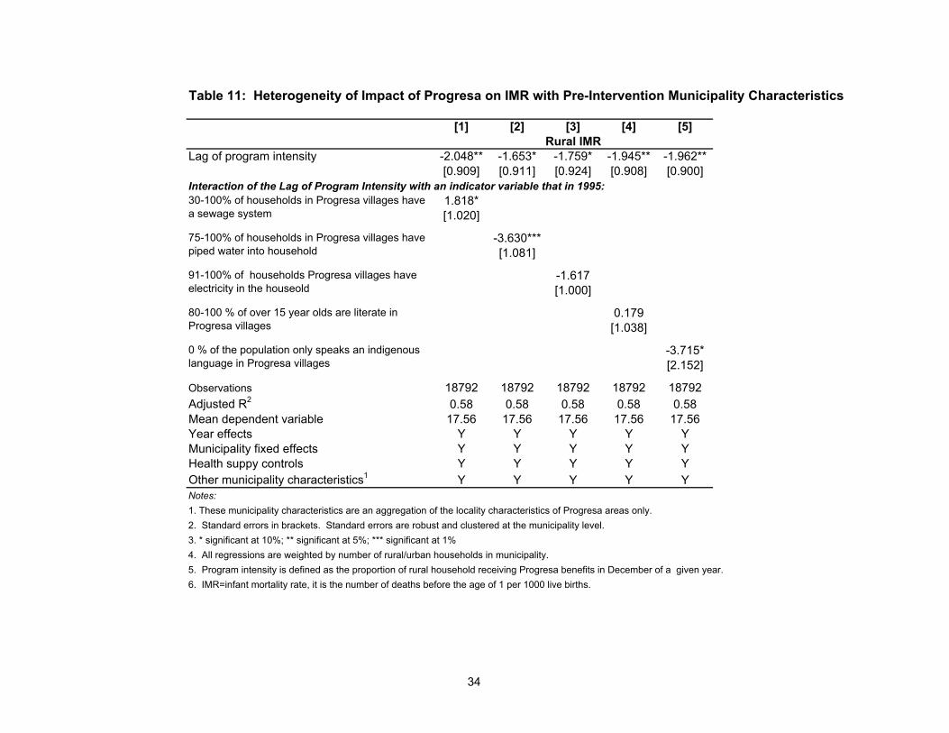
Table 11: Heterogeneity of Impact of Progresa on IMR with Pre-Intervention Municipality Characteristics

[1] [2] [3] [4] [5]

Lag of program intensity -2.048** -1.653* -1.759* -1.945** -1.962**[0.909] [0.911] [0.924] [0.908] [0.900]

Interaction of the Lag of Program Intensity with an indicator variable that in 1995:1.818*[1.020]

-3.630***[1.081]

-1.617[1.000]

0.179[1.038]

-3.715*[2.152]

Observations 18792 18792 18792 18792 18792Adjusted R2 0.58 0.58 0.58 0.58 0.58Mean dependent variable 17.56 17.56 17.56 17.56 17.56Year effects Y Y Y Y YMunicipality fixed effects Y Y Y Y YHealth suppy controls Y Y Y Y YOther municipality characteristics1 Y Y Y Y YNotes:1. These municipality characteristics are an aggregation of the locality characteristics of Progresa areas only.2. Standard errors in brackets. Standard errors are robust and clustered at the municipality level.3. * significant at 10%; ** significant at 5%; *** significant at 1%4. All regressions are weighted by number of rural/urban households in municipality.5. Program intensity is defined as the proportion of rural household receiving Progresa benefits in December of a given year.6. IMR=infant mortality rate, it is the number of deaths before the age of 1 per 1000 live births.

Rural IMR

30-100% of households in Progresa villages have a sewage system

75-100% of households in Progresa villages have piped water into household

0 % of the population only speaks an indigenous language in Progresa villages

91-100% of households Progresa villages have electricity in the houseold

80-100 % of over 15 year olds are literate in Progresa villages

34

35

Figure 1: Trends in the Number of Progresa Beneficiary Families and Localities

0

500

1000

1500

2000

2500

3000

1997 1998 1999 2000 2001Year

Num

ber o

f Rur

al

bene

ficia

ries

in 1

000s

0

10

20

30

40

50

60

70

Num

ber o

f rur

al

loca

litie

s in

100

0s

Rural Beneficiaries Rural Localities

Figure 2: Number of New Program Municipalities by Year

119

1318

644

12118

0

200

400

600

800

1000

1200

1400

1997 1998 1999 2000 2001

Year

Num

ber o

f Mun

icip

aliti

es

36

Figure 3: Trends in Rural IMR for Municipalities That Enter the Program in 1997

8

10

12

14

16

18

1992 1993 1994 1995 1996 1997 1998 1999 2000 2001

Year

IMR

Rural IMR Upper and Lower CI

Figure 5: Trends in Rural IMR for Municipalities That Enter the Program in 1999

8

10

12

14

16

18

20

1992 1993 1994 1995 1996 1997 1998 1999 2000 2001

Year

IMR

Rural IMR Upper and Lower CI

Figure 4: Trends in Rural IMR for Municipalities That Entered the Program in 1998

8

10

12

14

16

18

1992 1993 1994 1995 1996 1997 1998 1999 2000 2001

Year

IMR

Rural IMR Upper and Lower CI

Figure 6: Trends in Urban IMR by Year Municipality Entered Program

1012141618202224

1992 1993 1994 1995 1996 1997 1998 1999 2000 2001

Year

IMR

1997 1998 1999

37

Figure 7: Trends in Rural IMR by Municipality Entry Date

10

12

14

16

18

1992 1993 1994 1995 1996 1997 1998 1999 2000 2001

Year

IMR

1997 1998 1999

Note: Only municipalities with an average program intensity of at least 30% included.