PROVENANCE AND UNCERTAINTYSudeepa Roy

A DISSERTATION

in

Computer and Information Science

Presented to the Faculties of the University of Pennsylvania

in

Partial Fulfillment of the Requirements for the

Degree of Doctor of Philosophy

2012

Supervisor of Dissertation Supervisor of Dissertation

Signature Signature

Susan B. Davidson, Professor Sanjeev Khanna, Professor

Computer and Information Science Computer and Information Science

Graduate Group Chairperson

Signature

Jianbo Shi, Professor, Computer and Information Science

Dissertation Committee

Val Tannen, Professor, Computer and Information Science (Chair)

Andreas Haeberlen, Assistant Professor, Computer and Information Science

Zachary G. Ives, Associate Professor, Computer and Information Science

Tova Milo, Professor, School of Computer Science, Tel Aviv University (External)

Christopher Re, Assistant Professor, Department of Computer Sciences,

University of Wisconsin-Madison (External)

All rights reserved

INFORMATION TO ALL USERSThe quality of this reproduction is dependent upon the quality of the copy submitted.

In the unlikely event that the author did not send a complete manuscriptand there are missing pages, these will be noted. Also, if material had to be removed,

a note will indicate the deletion.

Microform Edition © ProQuest LLC.All rights reserved. This work is protected against

unauthorized copying under Title 17, United States Code

ProQuest LLC.789 East Eisenhower Parkway

P.O. Box 1346Ann Arbor, MI 48106 - 1346

UMI 3542930

Published by ProQuest LLC (2012). Copyright in the Dissertation held by the Author.

UMI Number: 3542930

PROVENANCE AND UNCERTAINTY

COPYRIGHT

2012

Sudeepa Roy

To

my parents and my husband

iii

Acknowledgements

This thesis would not have been possible without the generous help and support from

my professors, colleagues, friends, and family. I humbly extend my heartfelt gratitude to

all of them, and sincerely apologize to any of them who I forget to name here.

First and foremost, I thank my advisors Susan Davidson and Sanjeev Khanna, who

taught me how to do research: right from selecting problems to improving the written

and oral presentation of results. Their doors were always open in spite of their incredibly

busy schedule, and I was always fortunate to get their support in academic matters and

beyond.

I thank my dissertation committee members Andreas Haeberlen, Zack Ives, Tova Milo,

Chris Re, and Val Tannen, who graciously agreed to serve on the committee. They helped

me improve the presentation immensely with thoughtful and objective suggestions right

from when I submitted my thesis proposal.

The work presented in this dissertation is a result of an extensive and fruitful collabo-

ration with my advisors, and also with Laura Chiticariu, Vitaly Feldman, Tova Milo, Deb-

malya Panigrahi, Vittorio Perduca, Frederick Reiss, Val Tannen, and Huaiyu Zhu. Their

expertise in a diverse set of areas like algorithms and theory, databases and systems, and

machine learning enriched my knowledge and broadened my interests as a computer

scientist. I gratefully acknowledge their contributions in realizing this dissertation.

I sincerely thank Val Tannen, who has been a close collaborator, a mentor, and an

informal advisor to me. Val gave me far more attention and advice than I could have

asked for, and patiently suggested ways to overcome my shortcomings and consolidate

my strengths. My thanks to Tova Milo who was a wonderful collaborator and great source

of support. My research experience would not have been the same if I did not have the

opportunity to work with Tova and Val, who mentored me, made each research meeting

tremendously enjoyable, and helped me get a toe-hold in the academic community.

I was fortunate to be mentored and advised by a number of eminent researchers from

different fields. My heartfelt thanks to Laura Chiticariu, Julia Chuzhoy, Sudipto Guha,

Zack Ives, Sampath Kannan, Benny Kimelfeld, Wang-Chiew Tan, and Cong Yu, whose

iv

every bit of advice enhanced my experience as a graduate student. My sincere gratitude

to my advisors, Manindra Agrawal and Somenath Biswas, at IIT Kanpur who encouraged

me to join a doctoral program in the first place.

I thank all the members of the vibrant database group at Penn, especially Allen, Julia,

Ling, Marie, Medha, Mengmeng, Nan, Svilen, and Zhuowei, for giving me comments on

my research directions, being critical yet immensely helpful during practice talks, and

making my overall experience at Penn so enjoyable. Thanks to the administrative and

business staff who were always there to take care of administrative issues. My heartfelt

thanks are to Mike Felker, who is the one-stop solution for all matters in the department.

I do not have enough words to thank Annie and Marie, who were my closest friends,

confidants, and my immediate source of support, encouragement, and criticism, in the

last five years. We started our journey as a PhD student together five years back, and since

then I have shared every single achievement and failure with them, and have fallen back

on them for any need, whether academic or personal. Our gang of girls was strengthened

when Medha and Nan joined us last year, who have since wholesomely added to my life. I

have been blessed with a number of very close friends. I thank Aditi, Anirban (Basu and

Dey), Arindam, Arnab, Barna, Chandan, Debarghya, Dipanjan, Joydeep, Lakhsminath,

Maunendra, Payel, Sagarmoy, Sayak, Shaon, Shubhankar, Srobona, Subhendu, Sumit,

Supratim, Sunny, Varun, Vinaya, and all my other friends, for always being with me.

I could not have reached here without the unconditional love and support from my

family. My parents Sumita Roy and Sushanta Kumar Roy, my dear sister Urmimala,

uncles, aunts, and grandparents had unwavering belief in me and were overjoyed at my

tiniest achievements. I thank my parents-in-law, who are always more concerned than

I am about my health, happiness and professional career. My grandmother would have

been the happiest person today, and her memories will drive me in life forever. Last

but not the least, I do not know how to thank my loving husband Debmalya in words.

He is my best friend, colleague, and collaborator, my strongest source of support and

encouragement, and a pillar of strength at times of sorrow and desperation who can

change it to a smile in no time. I can only thank him by making our days to come

rewarding and full of happiness for both of us.

v

ABSTRACT

PROVENANCE AND UNCERTAINTYSudeepa Roy

Susan B. Davidson

Sanjeev Khanna

Data provenance, a record of the origin and transformation of data, explains how out-

put data is derived from input data. This dissertation focuses on exploring the connection

between provenance and uncertainty in two main directions: (1) how a succinct represen-

tation of provenance can help infer uncertainty in the input or the output, and (2) how

introducing uncertainty can facilitate publishing provenance information while hiding

associated private information.

A significant fraction of the data found in practice is imprecise, unreliable, and in-

complete, and therefore uncertain. The level of uncertainty in the data must be measured

and recorded in order to estimate the confidence in the results and find potential sources

of error. In probabilistic databases, uncertainty in the input is recorded as a probability

distribution, and the goal is to efficiently compute the induced probability distribution

on the outputs. In general, this problem is computationally hard, and we seek to expand

the class of inputs for which efficient evaluation is possible by exploiting provenance

structure.

In some scenarios, the output data is directly examined for errors and is labeled accord-

ingly. We need to trace back the errors in the output to the input so that the input can be

refined for future processing. Because of incomplete labeling of the output and complex-

ity of the processes generating it, the sources of error may be uncertain. We formalize

the problem of source refinement, and propose models and solutions using provenance

that can handle incomplete labeling. We also evaluate our solutions empirically for an

application of source refinement in information extraction.

Data provenance is extensively used to help understand and debug scientific exper-

iments that often involve proprietary and sensitive information. In this dissertation, we

consider privacy of proprietary and commercial modules when they belong to a work-

vi

flow and interact with other modules. We propose a model for module privacy that makes

the exact functionality of the modules uncertain by selectively hiding provenance infor-

mation. We also study the optimization problem of minimizing the information hidden

while guaranteeing a desired level of privacy.

vii

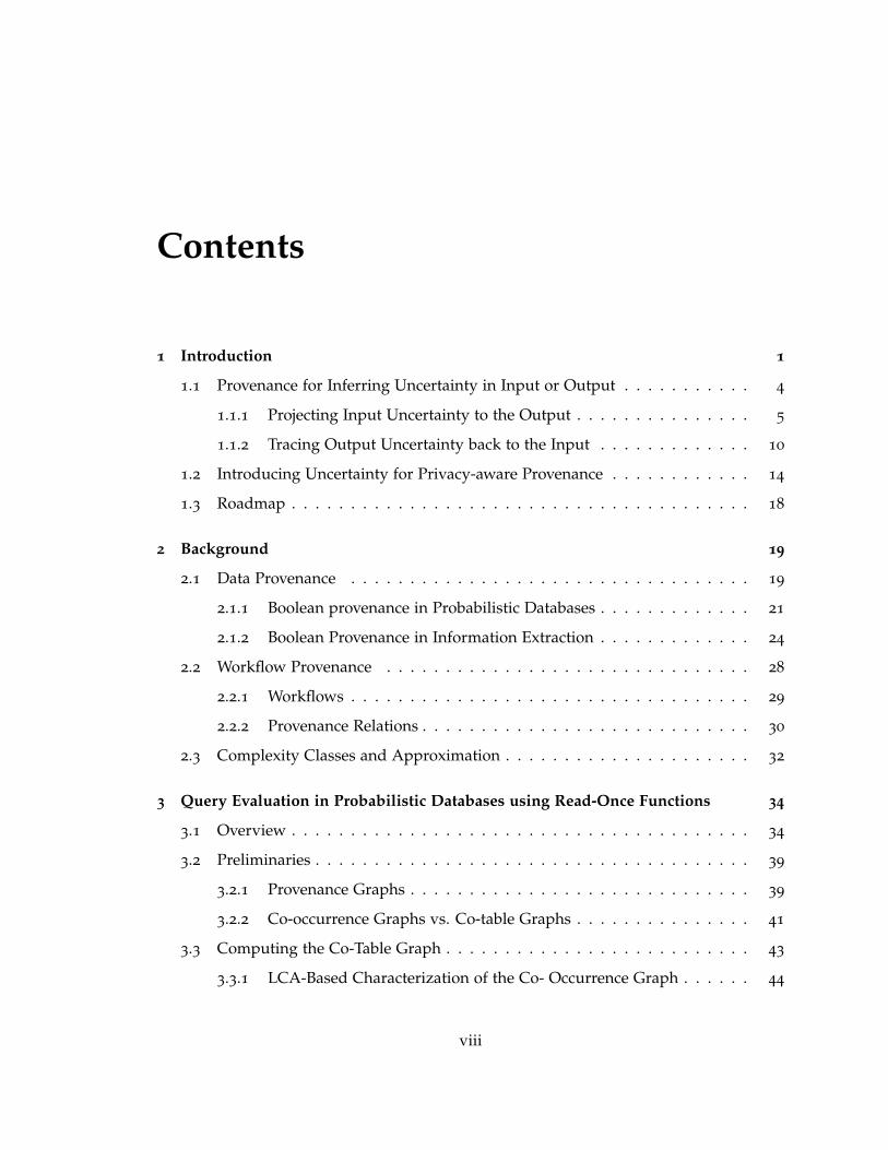
Contents

1 Introduction 1

1.1 Provenance for Inferring Uncertainty in Input or Output . . . . . . . . . . . 4

1.1.1 Projecting Input Uncertainty to the Output . . . . . . . . . . . . . . . 5

1.1.2 Tracing Output Uncertainty back to the Input . . . . . . . . . . . . . 10

1.2 Introducing Uncertainty for Privacy-aware Provenance . . . . . . . . . . . . 14

1.3 Roadmap . . . . . . . . . . . . . . . . . . . . . . . . . . . . . . . . . . . . . . . 18

2 Background 19

2.1 Data Provenance . . . . . . . . . . . . . . . . . . . . . . . . . . . . . . . . . . 19

2.1.1 Boolean provenance in Probabilistic Databases . . . . . . . . . . . . . 21

2.1.2 Boolean Provenance in Information Extraction . . . . . . . . . . . . . 24

2.2 Workflow Provenance . . . . . . . . . . . . . . . . . . . . . . . . . . . . . . . 28

2.2.1 Workflows . . . . . . . . . . . . . . . . . . . . . . . . . . . . . . . . . . 29

2.2.2 Provenance Relations . . . . . . . . . . . . . . . . . . . . . . . . . . . . 30

2.3 Complexity Classes and Approximation . . . . . . . . . . . . . . . . . . . . . 32

3 Query Evaluation in Probabilistic Databases using Read-Once Functions 34

3.1 Overview . . . . . . . . . . . . . . . . . . . . . . . . . . . . . . . . . . . . . . . 34

3.2 Preliminaries . . . . . . . . . . . . . . . . . . . . . . . . . . . . . . . . . . . . . 39

3.2.1 Provenance Graphs . . . . . . . . . . . . . . . . . . . . . . . . . . . . . 39

3.2.2 Co-occurrence Graphs vs. Co-table Graphs . . . . . . . . . . . . . . . 41

3.3 Computing the Co-Table Graph . . . . . . . . . . . . . . . . . . . . . . . . . . 43

3.3.1 LCA-Based Characterization of the Co- Occurrence Graph . . . . . . 44

viii

3.3.2 Computing the Table-Adjacency Graph . . . . . . . . . . . . . . . . . 46

3.3.3 Computing the Co-Table Graph . . . . . . . . . . . . . . . . . . . . . 46

3.4 Computing the Read-Once Form . . . . . . . . . . . . . . . . . . . . . . . . . 48

3.4.1 Algorithm CompRO . . . . . . . . . . . . . . . . . . . . . . . . . . . . 49

3.5 Discussion . . . . . . . . . . . . . . . . . . . . . . . . . . . . . . . . . . . . . . 56

3.6 Related Work . . . . . . . . . . . . . . . . . . . . . . . . . . . . . . . . . . . . 59

3.7 Conclusions . . . . . . . . . . . . . . . . . . . . . . . . . . . . . . . . . . . . . 60

4 Queries with Difference on Probabilistic Databases 63

4.1 Overview . . . . . . . . . . . . . . . . . . . . . . . . . . . . . . . . . . . . . . . 63

4.2 Preliminaries . . . . . . . . . . . . . . . . . . . . . . . . . . . . . . . . . . . . . 67

4.2.1 Difference Rank . . . . . . . . . . . . . . . . . . . . . . . . . . . . . . . 67

4.2.2 Read-Once and d-DNNF . . . . . . . . . . . . . . . . . . . . . . . . . 68

4.2.3 From Graphs to Queries . . . . . . . . . . . . . . . . . . . . . . . . . . 70

4.3 Hardness of Exact Computation . . . . . . . . . . . . . . . . . . . . . . . . . 71

4.4 Approximating Tuple Probabilities . . . . . . . . . . . . . . . . . . . . . . . . 73

4.4.1 Probability-Friendly Form (PFF) . . . . . . . . . . . . . . . . . . . . . 74

4.4.2 PFF and General Karp-Luby Framework . . . . . . . . . . . . . . . . 74

4.4.3 FPRAS to Approximate Tuple Probabilities . . . . . . . . . . . . . . . 75

4.4.4 Classes of Queries Producing PFF . . . . . . . . . . . . . . . . . . . . 79

4.5 Related Work . . . . . . . . . . . . . . . . . . . . . . . . . . . . . . . . . . . . 80

4.6 Conclusions . . . . . . . . . . . . . . . . . . . . . . . . . . . . . . . . . . . . . 80

5 Provenance-based Approach for Dictionary Refinement in Information Extrac-

tion 82

5.1 Overview . . . . . . . . . . . . . . . . . . . . . . . . . . . . . . . . . . . . . . . 82

5.2 Dictionary Refinement Problem . . . . . . . . . . . . . . . . . . . . . . . . . . 87

5.2.1 Estimating Labels of Results for Sparse Labeling . . . . . . . . . . . 88

5.2.2 Formal Problem Definition . . . . . . . . . . . . . . . . . . . . . . . . 89

5.3 Estimating Labels . . . . . . . . . . . . . . . . . . . . . . . . . . . . . . . . . . 91

5.3.1 The Statistical Model . . . . . . . . . . . . . . . . . . . . . . . . . . . . 91

ix

5.3.2 Estimating Labels from Entry-Precisions . . . . . . . . . . . . . . . . 92

5.3.3 Estimating Entry-Precisions by EM . . . . . . . . . . . . . . . . . . . 92

5.4 Refinement Optimization . . . . . . . . . . . . . . . . . . . . . . . . . . . . . 94

5.4.1 Refinement Optimization for Single Dictionary . . . . . . . . . . . . 95

5.4.2 Refinement Optimization for Multiple Dictionaries . . . . . . . . . . 100

5.5 Experiments . . . . . . . . . . . . . . . . . . . . . . . . . . . . . . . . . . . . . 102

5.5.1 Evaluation Datasets . . . . . . . . . . . . . . . . . . . . . . . . . . . . 103

5.5.2 Dictionary Refinement with Full Labeling . . . . . . . . . . . . . . . 104

5.5.3 Dictionary Refinement with Incomplete Labeling . . . . . . . . . . . 107

5.6 Related Work . . . . . . . . . . . . . . . . . . . . . . . . . . . . . . . . . . . . 111

5.7 Conclusions . . . . . . . . . . . . . . . . . . . . . . . . . . . . . . . . . . . . . 113

6 Provenance Views for Module Privacy 114

6.1 Overview . . . . . . . . . . . . . . . . . . . . . . . . . . . . . . . . . . . . . . . 115

6.2 Module Privacy . . . . . . . . . . . . . . . . . . . . . . . . . . . . . . . . . . . 117

6.2.1 Standalone Module Privacy . . . . . . . . . . . . . . . . . . . . . . . . 118

6.3 Standalone Module Privacy . . . . . . . . . . . . . . . . . . . . . . . . . . . . 122

6.3.1 Lower Bounds . . . . . . . . . . . . . . . . . . . . . . . . . . . . . . . . 123

6.3.2 Upper Bounds . . . . . . . . . . . . . . . . . . . . . . . . . . . . . . . 125

6.4 All-Private Workflows . . . . . . . . . . . . . . . . . . . . . . . . . . . . . . . 126

6.4.1 Standalone-Privacy vs. Workflow-Privacy . . . . . . . . . . . . . . . 127

6.4.2 The Secure-View Problem . . . . . . . . . . . . . . . . . . . . . . . 131

6.4.3 Complexity results . . . . . . . . . . . . . . . . . . . . . . . . . . . . . 133

6.5 Public Modules . . . . . . . . . . . . . . . . . . . . . . . . . . . . . . . . . . . 137

6.5.1 Standalone vs. Workflow Privacy (Revisited) . . . . . . . . . . . . . . 137

6.5.2 The Secure-View Problem (Revisited) . . . . . . . . . . . . . . . . . 140

6.6 Related Work . . . . . . . . . . . . . . . . . . . . . . . . . . . . . . . . . . . . 140

6.7 Conclusions . . . . . . . . . . . . . . . . . . . . . . . . . . . . . . . . . . . . . 142

7 A Propagation Model for Module Privacy 144

7.1 Overview . . . . . . . . . . . . . . . . . . . . . . . . . . . . . . . . . . . . . . . 144

x

7.2 Privacy via propagation . . . . . . . . . . . . . . . . . . . . . . . . . . . . . . 148

7.2.1 Upward vs. downward propagation . . . . . . . . . . . . . . . . . . . 149

7.2.2 Recursive propagation . . . . . . . . . . . . . . . . . . . . . . . . . . . 150

7.2.3 Selection of hidden attributes . . . . . . . . . . . . . . . . . . . . . . . 151

7.3 Privacy for Single-Predecessor workflows . . . . . . . . . . . . . . . . . . . . 154

7.3.1 Proof of the Privacy Theorem . . . . . . . . . . . . . . . . . . . . . . . 154

7.3.2 Necessity of Single-Predecessor Assumption . . . . . . . . . . . . . . 161

7.4 Optimization . . . . . . . . . . . . . . . . . . . . . . . . . . . . . . . . . . . . . 162

7.4.1 Optimization in Four Steps . . . . . . . . . . . . . . . . . . . . . . . . 163

7.4.2 Solutions for Individual Modules . . . . . . . . . . . . . . . . . . . . 165

7.4.3 Optimization: Single Private Module . . . . . . . . . . . . . . . . . . 166

7.5 General Workflows . . . . . . . . . . . . . . . . . . . . . . . . . . . . . . . . . 169

7.6 Conclusion . . . . . . . . . . . . . . . . . . . . . . . . . . . . . . . . . . . . . . 170

8 Conclusions 172

A Additional Details and Proofs 176

A.1 Proofs from Chapter 3 . . . . . . . . . . . . . . . . . . . . . . . . . . . . . . . 176

A.2 Proofs from Chapter 4 . . . . . . . . . . . . . . . . . . . . . . . . . . . . . . . 190

A.3 Proofs from Chapter 5 . . . . . . . . . . . . . . . . . . . . . . . . . . . . . . . 201

A.4 Proofs from Chapter 6 . . . . . . . . . . . . . . . . . . . . . . . . . . . . . . . 209

A.5 Proofs from Chapter 7 . . . . . . . . . . . . . . . . . . . . . . . . . . . . . . . 233

Bibliography 271

xi

List of Tables

1.1 Complexity of exact and approximate computation of probability for dif-

ference of two positive queries (CQ = conjunctive query, UCQ = Union of

conjunctive query). . . . . . . . . . . . . . . . . . . . . . . . . . . . . . . . . . 10

7.1 Relation R for workflow given in Figure 7.3a . . . . . . . . . . . . . . . . . . 157

7.2 Relation R′, a possible world of the relation R for the workflow in Fig-

ure 7.3a w.r.t. V = a1, a2, a6. . . . . . . . . . . . . . . . . . . . . . . . . . . . 160

7.3 Relation Ra for workflow Wa given in Figure 7.3b . . . . . . . . . . . . . . . 161

A.1 Relation Rb for workflow Wb given in Figure A.5a . . . . . . . . . . . . . . . 249

A.2 Relation Rd for workflow Wd given in Figure A.5. . . . . . . . . . . . . . . . 250

xii

List of Illustrations

1.1 A database instance I with three relations R,S, and T, query q, and Boolean

provenance of the output tuples. . . . . . . . . . . . . . . . . . . . . . . . . . 5

1.2 Input relations UserGroup, GroupAccess, and output relation UserAccess

with correct/incorrect labeling on the output tuples. . . . . . . . . . . . . . 12

2.1 A tuple-independent probabilistic database I with three input relations

R,S, T, where the tuples are annotated with tuple variables and probabilities. 21

2.2 A safe query q and Boolean provenance of the output tuples in q(I). . . . . 22

2.3 An unsafe query q′ and Boolean provenance of the output tuples in q′(I). . 23

2.4 Example Person Extractor with Input Document, rules, dictionaries and

intermediate and output views. . . . . . . . . . . . . . . . . . . . . . . . . . . 25

2.5 An example workflow, and module and workflow executions as prove-

nance relations . . . . . . . . . . . . . . . . . . . . . . . . . . . . . . . . . . . 30

3.1 A tuple-independent probabilistic database where the tuples are annotated

with tuple variables and probabilities. . . . . . . . . . . . . . . . . . . . . . . 35

3.2 Provenance graph for R ./ S. . . . . . . . . . . . . . . . . . . . . . . . . . . . 40

3.3 Provenance graph for π()((R ./ S) ./ T). . . . . . . . . . . . . . . . . . . . . . 40

3.4 Co-occurrence graph Gco for the Boolean provenance f in Example 3.2. . . 41

3.5 Table-adjacency graph GT for the relations in Example 3.2. . . . . . . . . . . 42

3.6 Co-table graph GC for the Boolean provenance f in Example 3.2. . . . . . . 43

3.7 GC,1 and GC,2. . . . . . . . . . . . . . . . . . . . . . . . . . . . . . . . . . . . . 54

3.8 Marked table-adjacency graph for R,S, T. . . . . . . . . . . . . . . . . . . . . 56

xiii

4.1 Boolean provenance for the query q− q′. . . . . . . . . . . . . . . . . . . . . 64

4.2 φ = u1(v1 + v2) + u3v4: (a) as a read-once tree, (b) as a d-DNNF. . . . . . . 69

5.1 Details of evaluation data sets . . . . . . . . . . . . . . . . . . . . . . . . . . . 104

5.2 Histograms for statistics of the data : (i) Fraction of bad results produced

by entries and relative frequencies of entries, (ii) Count of bad results pro-

duced by entries. . . . . . . . . . . . . . . . . . . . . . . . . . . . . . . . . . . 105

5.3 Performance of refinement optimization algorithms for single dictionary:

(i) Size constraint, (ii) Recall constraint . . . . . . . . . . . . . . . . . . . . . 106

5.4 Running times of refinement algorithms for single dictionary : (i) Size con-

straint, (ii) Recall constraint . . . . . . . . . . . . . . . . . . . . . . . . . . . . 107

5.5 Refinement algorithms for multiple dictionary: (i) Size Vs. F-score, (ii)

Recall budget Vs. F-score . . . . . . . . . . . . . . . . . . . . . . . . . . . . . 108

5.6 Running time for multiple dictionary (i) Size Vs. Time, (ii) Recall Budget

Vs. Time . . . . . . . . . . . . . . . . . . . . . . . . . . . . . . . . . . . . . . . 109

5.7 Effect of the labeled data size on F-score for single dictionary (i) Size con-

straint, (ii) Recall constraint. . . . . . . . . . . . . . . . . . . . . . . . . . . . 110

5.8 Effect of the labeled data size on F-score for multiple dictionary (i) Size

constraint, (ii) Recall constraint. . . . . . . . . . . . . . . . . . . . . . . . . . 111

5.9 Top 10 entries output by the (near) optimal algorithms for size and recall

constraints. . . . . . . . . . . . . . . . . . . . . . . . . . . . . . . . . . . . . . . 112

6.1 (a): Projected relation for m1 when attribute a2, a4 are hidden, (b)-(d):

Ri1 ∈ Worlds(R1,V), i ∈ [1,4] . . . . . . . . . . . . . . . . . . . . . . . . . . . 119

6.2 IP for Secure-View with cardinality constraints . . . . . . . . . . . . . . . 134

7.1 A single-predecessor workflow. White modules are public, grey are private;

the box denotes the composite module M for V2 = a2. . . . . . . . . . . . 151

7.2 UD-safe solutions for modules . . . . . . . . . . . . . . . . . . . . . . . . . . 152

7.3 White modules are public, grey are private. . . . . . . . . . . . . . . . . . . . 156

A.1 Illustration with n = 3, E3 = x1x2 + x2x3 + x3x4. . . . . . . . . . . . . . . . . 177

xiv

A.2 Reduction from label cover: bold edges correspond to (p,q) ∈ Ruw, dotted

edges are for data sharing. . . . . . . . . . . . . . . . . . . . . . . . . . . . . . 224

A.3 Reduction from vertex cover, the dark edges show a solution with cost

|E′|+ K, K = size of a vertex cover in G′ . . . . . . . . . . . . . . . . . . . . . 226

A.4 Reduction from label cover: (p,q) ∈ Ruw, the public modules are darken,

all public modules have unit cost, all data have zero cost, the names of the

data never hidden are omitted for simplicity . . . . . . . . . . . . . . . . . . 230

A.5 White modules are public, Grey are private. . . . . . . . . . . . . . . . . . . 249

A.6 Reduction from 3SAT. Module p0 is private, the rest are public. The narrow

dark edges (in red) denote TRUE assignment, the bold dark edges (in blue)

denote FALSE assignment. . . . . . . . . . . . . . . . . . . . . . . . . . . . . . 262

xv

Chapter 1

Introduction

Data provenance (also known as lineage or pedigree) is a record of origin and transforma-

tion of data [33]. Data provenance, which explains how the output data is derived from

the input data in an experiment, simulation, or query evaluation, has been extensively

studied over the last decade. Its applications include data cleaning, sharing, and integra-

tion [46, 99, 166], data warehousing [51], transport of annotations between data sources

and views [34], view update and maintenance [18, 34, 44, 81, 87, 88, 173], verifiability and

debugging in scientific workflows [19, 24, 27, 128, 158] and business processes [53, 69],

and so on. Various tools and frameworks have been proposed to support provenance in

these applications [32, 99, 175].

The central focus of this dissertation is to explore the connection between provenance and

uncertainty. A significant fraction of data found in practice is imprecise, unreliable, and

incomplete, which leads to uncertainty in data. For example, RFID sensor data in wireless

sensor networks is often noisy due to environmental interference, inherent measurement

noise, and sensor failures. Similarly, data collected by surveys or crowd-sourced platforms

like Amazon Mechanical Turk [1] is uncertain because of variations in taste, opinion,

and the level of effort put in by the crowd in generating the data. In addition, some

information may be lost or introduced when data undergoes multiple transformations

and is stored in different formats.

In any practical application, it is important to measure and record the level of un-

certainty in the data in order to estimate the confidence in the results obtained, or find

1

potential sources of errors. Uncertainty can be recorded either in the source or in the

output. In applications like sensor networks, it is well-known that RFID sensors often

record inaccurate values. Therefore, multiple sensors are usually deployed for the same

task, e.g., recording the temperature of a room. Based on the values these sensors record,

we obtain a probability distribution over a range of temperatures. This is an example of

recording uncertainty in the source. Further processing of the recorded temperatures (e.g.,

finding whether the room temperature was greater than a certain threshold at any time

of a day) induces a probability distribution on the possible outputs.

In some scenarios, we do not have a prior measure of confidence on the source data,

whereas the output data can be directly examined for errors and is labeled accordingly.

For instance, in the above example, an independent observer may certify that the room

temperature was always lower than the given threshold, whereas the sensors recorded

otherwise. In this case, the sensor recordings are labeled as incorrect. It is important that

this (often incompletely) labeled output data is now used to identify the faulty sensors

for rectification or removal.

The above examples motivate the first part of this dissertation. Here we study appli-

cations of provenance, i.e. how the output was generated from the input, in inferring

uncertainty in the input or the output data. The framework of projecting uncertainty in

the input, specified as probability distributions, to the output has been widely studied

in the field of probabilistic databases [161]. Here the main challenge is to compute the

probability distribution on the possible output values as efficiently as possible for a large

input data set. We use a certain form of provenance, that we call Boolean provenance, to

efficiently compute the exact or approximate probabilities of the outputs. It has been

shown in the literature that there is a class of “hard” positive relational queries (involving

SELECT-PROJECT-JOIN-UNION operators) that are not amenable to efficient computa-

tion of output probabilities on some instances. Our first contribution is to efficiently

identify a natural class of query-database instance pairs that allow efficient computation of

the output probabilities even if the query is hard. Our second contribution is to initiate

the study of queries that involve the set difference operator (EXCEPT or MINUS in SQL),

which adds substantial complexity to the class of positive queries.

2

Conversely, for tracing uncertainty in the output back to the input, we also use Boolean

provenance. The goal is to refine the source, i.e. find and remove inputs that are respon-

sible for producing many incorrect outputs. However, the same input might produce

a combination of correct and incorrect outputs. So we must ensure that refining the

inputs does not delete a significant number of correct outputs. We formalize the prob-

lem of balancing incorrect outputs retained and correct outputs deleted by the process

of source refinement, and propose efficient algorithmic solutions for this problem. We

also address the problem of incomplete labeling of the output by proposing a statisti-

cal model that helps predict the missing labels using techniques from machine learning.

Our approach of source refinement is discussed via an important application in informa-

tion extraction where we also evaluate our solutions empirically on a real-life information

extraction system [114].

In general, data provenance helps understand and debug an experiment, transaction,

or query evaluation in scientific, medical, or pharmaceutical research and business pro-

cesses [19, 24, 27, 53, 69, 128, 158]. Workflows, which capture processes and data flows in

these domains, constitute a critical component of experiments like genome sequencing,

protein folding, phylogenetic tree construction, clinical trials, drug design and synthe-

sis, etc. Due to substantial investments in developing a workflow and its components,

which also often includes proprietary or sensitive elements (e.g., medical information,

proprietary algorithms, etc), organizations may wish to keep certain details private while

publishing the provenance information.

The second part of this dissertation focuses on module privacy for proprietary and com-

mercial modules when they combine with other modules in a workflow in order to com-

plete a task. Unlike the first part of the dissertation where we use provenance to infer

uncertainty in the input or the output, we intentionally introduce uncertainty in provenance

to protect functionality of the private modules. Arbitrary network structure and interac-

tion with other modules in a workflow make it difficult to guarantee desired privacy

levels for proprietary modules. Here we show that we can find private solutions locally

for individual modules and combine them to ensure privacy of modules in a workflow

irrespective of its structure. Naturally, there is a tension between publishing accurate

3

provenance information and privacy of modules. So our algorithms aim to minimize the

provenance information hidden while ensuring a required privacy level. We also argue

that the guarantees provided by our algorithms are essentially the best possible.

In view of the above discussion, we now describe two main directions in this dis-

sertation connecting provenance and uncertainty: (i) how a succinct representation of

provenance can help infer uncertainty in the input or the output (Section 1.1), and (ii)

how uncertainty can facilitate privacy-aware provenance (Section 1.2). In these sections,

we briefly review the relevant previous approaches, discuss how we use provenance to

address the underlying challenges, and summarize our technical contributions.

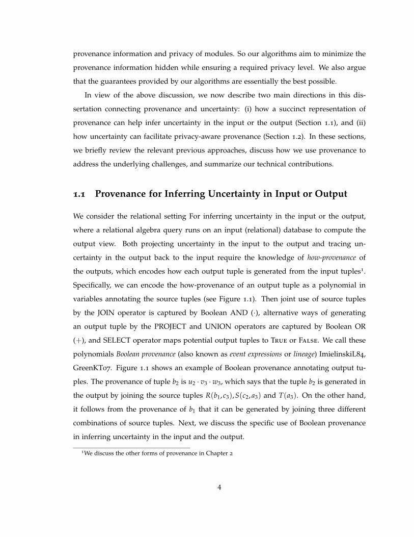
1.1 Provenance for Inferring Uncertainty in Input or Output

We consider the relational setting For inferring uncertainty in the input or the output,

where a relational algebra query runs on an input (relational) database to compute the

output view. Both projecting uncertainty in the input to the output and tracing un-

certainty in the output back to the input require the knowledge of how-provenance of

the outputs, which encodes how each output tuple is generated from the input tuples1.

Specifically, we can encode the how-provenance of an output tuple as a polynomial in

variables annotating the source tuples (see Figure 1.1). Then joint use of source tuples

by the JOIN operator is captured by Boolean AND (·), alternative ways of generating

an output tuple by the PROJECT and UNION operators are captured by Boolean OR

(+), and SELECT operator maps potential output tuples to True or False. We call these

polynomials Boolean provenance (also known as event expressions or lineage) ImielinskiL84,

GreenKT07. Figure 1.1 shows an example of Boolean provenance annotating output tu-

ples. The provenance of tuple b2 is u2 · v3 ·w3, which says that the tuple b2 is generated in

the output by joining the source tuples R(b1, c3),S(c2, a3) and T(a3). On the other hand,

it follows from the provenance of b1 that it can be generated by joining three different

combinations of source tuples. Next, we discuss the specific use of Boolean provenance

in inferring uncertainty in the input and the output.

1We discuss the other forms of provenance in Chapter 2

4

R

b1 c1 u1

b2 c2 u2

b1 c3 u3

S

c1 a1 v1

c1 a2 v2

c2 a3 v3

c3 a2 v4

T

a1 w1

a2 w2

a3 w3

q(I)

b1 u1 · v1 · w1 + u1 · v2 · w2 + u3 · v4 · w2

b2 u2 · v3 · w3

q(x) : −R(x,y),S(y,z), T(z)

Figure 1.1: A database instance I with three relations R,S, and T, query q, and Boolean

provenance of the output tuples.

1.1.1 Projecting Input Uncertainty to the Output

Unreliable data sources, noisy data collectors (like sensor data), and multiple transforma-

tions and revisions inject uncertainty in data. Probabilistic databases enable us to capture,

model, and process uncertain data assuming a probability distribution on the possible

instances of the database. Query evaluation on probabilistic databases results in a proba-

bility distribution on possible outputs instead of a deterministic answer.

Boolean provenance in probabilistic databases. A standard and fundamental model

is to assume tuple-independent probabilistic databases. Here each source tuple realizes in

a random instance of the database with some probability independent of the other source

tuples. The Boolean variable annotating a source tuple correspond to the event that the

source tuple realizes, e.g. R(b1, c1) exists in a random instance of the database if and only

if u1 = True, and this event has a certain probability Pr[u1]. It can be easily seen that

an output tuple appears as a result of query evaluation on a random database instance

if and only if its Boolean provenance evaluates to True. Therefore, in tuple-independent

probabilistic databases, the probability of an output tuple equals the probability of its

Boolean provenance, e.g. Pr[b1 appears in q(I)] = Pr[u1 · v1 ·w1 + u1 · v2 ·w2 + u3 · v4 ·w2].

There are several reasons to use Boolean provenance for query evaluation in proba-

bilistic databases. First, the number of random instances of the input database can be

exponential in the number of source tuples with non-zero probability. Using Boolean

provenance saves the effort of dealing with all possible database instances, i.e. evaluating

the query on each such instance and summing up the probabilities of the instances that

5

gives the intended output tuple2. Second, evaluating the probability of a Boolean expres-

sion from the probabilities of its constituent variables has been extensively studied in the

literature, and is closely related to computing the number of satisfying assignments of

a Boolean expression. This enables us to have a better understanding of the difficulties

in probability computation. Moreover, the Boolean provenance of the output tuples can

be computed without much overhead when a query is evaluated on an annotated source

database. The challenge in computing the probability distributions using Boolean prove-

nance appears in the next step. The problem of computing the probability of an arbitrary

Boolean expression from that of its constituent variables is directly related to counting

the number of satisfying assignments of the expression which is known to be computa-

tionally hard (#P-hard). Further, these hard expressions may be generated by very simple

queries. Therefore, the key challenge in probabilistic databases is to be able to efficiently

compute the probability distribution on the outputs for a large class of inputs.

Previous approaches. Dalvi et. al. have studied efficient computability of proba-

bility distribution on the outputs, and have given important dichotomy results for positive

relational algebra queries [54–57]. These results show that the set of such queries can be

divided into (i) the queries for which poly-time computation of output probability dis-

tribution is possible on all instances (called safe queries); and (ii) the queries for which

such computation is hard (called unsafe queries). There has been interesting progress in

other directions in probabilistic databases as well. Several systems for query processing

on probabilistic databases have been developed, including MistiQ [25], Trio [17, 174], and

MayBMS [10]. Significant work has been done on top-k queries [117, 144, 159] and aggre-

gate queries [146] on probabilistic databases. The relation between Boolean provenance

generated by safe queries and several knowledge compilation techniques has also been

explained [101, 137]. Frameworks have been proposed for exact and approximate evalua-

tion of the answers that work well in practice (but may not run in time polynomial in the

size of input database) [77, 100, 140]. A completely different approach models correla-

tions between tuples, compiles queries and databases into probabilistic graphical models

and then performs inference on these [149, 154, 155]. Another line of work has focused

2For some queries, explicit computation of the Boolean provenance is not needed and the probabilities of

the outputs can be directly computed while evaluating the query [54, 55].

6

on exploring more expressible query languages for probabilistic databases and their com-

putability. For instance, [68] considers datalog, fixpoint and “while” queries, where either

the state of the database changes after each evaluation of the query, or new results are

added to the answer set; [109] studies compositional use of confidence parameters in the

query such as selection based on marginal and conditional probabilities.

Our contributions. In view of the above state of the art, this dissertation considers

two simple yet fundamental questions. In Chapter 3, we extend the class of inputs (query-

database pairs) for which poly-time exact computation is possible, while in Chapter 4, we

enrich the class of queries studied in the literature by including the difference operations.

Here we give a technical summary of our contributions in these two chapters.

• Query Evaluation in Probabilistic Databases using Read-Once Functions

Chapter 3 is based on the results published in [152] (joint work with Vittorio Perduca

and Val Tannen). As mentioned earlier, safe queries are amenable to poly-time

computation for all input databases. However, the class of unsafe queries includes

very simple queries like q() : −R(x),S(x,y), T(y) and are unavoidable in practice.

Our observation is that, even for unsafe queries, there may be classes of “easy” data

inputs where the answer probabilities can be computed in polynomial time in the

size of the database: this we call the instance-by-instance approach. In particular, our

goal is efficiently identify the input query-database pairs where Boolean provenance

of an output is read-once.

A Boolean expression is in read-once form if each of its variables appears exactly once,

e.g. x(y+ z)3. The significance of a read-once expression is that its probability can be

computed in linear-time in the number of variables when the variables are mutually

independent (repeatedly use Pr[xy] = Pr[x]Pr[y] and Pr[x + y] = 1− (1− Pr[x])(1−

Pr[y])). However, there are expressions that are not in read-once form, but are read-

once, i.e. such an expression has an equivalent read-once form (e.g. xy + xz). Indeed,

there are non-read-once expressions as well (e.g. xy + yz + zx or xy + yz + zw). In

Figure 1.1 the provenance of b2 (i.e. u2v3w3) is read-once and also in read-once form,

while the provenance of b1 (i.e. u1v1w1 + u1v2w2 + u3v4w2) is not read-once. Our

3From now on, we will omit “·” to denote AND operation in Boolean expression for brevity.

7

goal in this chapter is to decide whether a Boolean provenance is read-once (and if

yes, to compute the read-once form) as efficiently as possible.

When the Boolean formula is given in “irredundant” disjunctive normal form (DNF)

(i.e. none of the disjuncts can be omitted using absorption like x + xy = x), there is

a fast algorithm by Golumbic et. al. [85] to decide whether a Boolean expression is

read-once. This algorithm is based upon a characterization given by Gurvich [91].

For positive relational queries, the size of the irredundant DNF for a Boolean prove-

nance is polynomial in the size of the table, but can be exponential in the size of

the query. On the other hand, often optimized query plans produce more compact

expressions, motivating the study of approaches that can avoid the explicit compu-

tation of these DNFs. However, DNF computation seems unavoidable for arbitrary

Boolean expressions. Hellerstein and Karpinski[97] have shown that given a mono-

tone Boolean formula defining a read-once function, the equivalent read-once form

cannot be computed in poly-time in the size of the formula unless NP = RP4.

In [152], we exploit special structures of Boolean provenance to avoid expanding

the expression into DNF. We show that for a large and important class of queries,

conjunctive queries without self-join, the existing characterization and algorithms can

be used to decide read-once-ness of arbitrary Boolean provenance (not necessarily

in irredundant DNF) by recording some additional information when the query is

evaluated. Moreover, using the properties of conjunctive queries without self-join,

we propose a simpler and asymptotically faster algorithm that also introduces a

novel characterization of the read-once Boolean provenance for this class of queries.

• Queries with Difference on Probabilistic Databases

Chapter 4 presents our results published in [106] (joint work with Sanjeev Khanna

and Val Tannen). Difference operations (e.g. EXCEPT, MINUS in SQL) are fre-

quently found in real-life queries, but the complexity of query evaluation with these

operations had not been studied previously for probabilistic databases. The concept

4The complexity class RP (Randomized Polynomial time) consists of the languages L having a polynomial-

time randomized algorithm that rejects all inputs not in L with probability 1, and accepts all inputs in L with

probability ≥ 1/2.

8

of Boolean provenance naturally extends to difference (see Chapter 4). However,

there are some new and considerable difficulties with such queries. For any posi-

tive query without difference operations, even if the exact computation is hard, the

well-known DNF-counting algorithm given by Karp and Luby [104] can be adapted

to approximate the probabilities upto any desired level of accuracy. But, for queries

with difference, the DNF of Boolean provenance is no longer monotone, and may be

exponential in the size of the database. This precludes using both the read-onceness

testing algorithm of [85], and also the approximation algorithm given by Karp and

Luby. In recent and independent work [77], Fink et. al. proposed a framework

to compute exact and approximate probabilities for answers of arbitrary relational

algebra queries that allow difference operations. However, there is no guarantee of

polynomial running time.

In this work, we study the complexity of computing the probability for queries

with difference on tuple-independent databases. (1) We exhibit two Boolean queries

q1 and q2, both of which independently have nice structures, namely they are safe

conjunctive queries without self-joins (i.e. allow poly-time computation on all in-

stances), but such that computing the probability of q1 − q2 is #P-hard. This hard-

ness of exact computation result suggests that any class of interesting queries with

difference which are safe in the spirit of [54–56] would have to be severely restricted5

(2) In view of this lower bound for exact computation, we give a Fully Polyno-

mial Randomized Approximation Scheme (FPRAS) for approximating probabilities for

a class of queries with difference. In particular, a corollary of our result applies to

queries of the form q1 − q2, where q1 is an arbitrary positive query while q2 is a

safe positive query without self-join. Our algorithm uses a new application of the

Karp-Luby framework [104] that goes well beyond DNF counting, and also works for

the instance-by-instance approach in the spirit of Chapter 3. (3) We show that the

latter restriction stated above is important: computing the probability of “True− q”

is inapproximable (no FPRAS exists) where True is the Boolean query that is always

true while q is the Boolean conjunctive query q() :− S(x), R(x,y),S(y). Table 1.1

5There is always the easy and uninteresting case when the events associated with q1 and with q2 are

independent of each other because, for example, they operate on separate parts of the input database.

9

Pr[q1 − q2]

q1 q2 Exact Approximate

UCQ safe CQ without self-join#P-hard

FPRAS

UCQ UCQ Inapproximable

Table 1.1: Complexity of exact and approximate computation of probability for difference

of two positive queries (CQ = conjunctive query, UCQ = Union of conjunctive query).

summarizes the three results for differences of positive queries. This work is a first

step to explore the complexity of queries with difference operation; an important

future direction in this area is to obtain a complete classification of these queries

(and Boolean provenance) in terms of their complexity.

1.1.2 Tracing Output Uncertainty back to the Input

In applications like information extraction (e.g., finding all instances of person names

from a document), database administration (e.g., curating source data in order to satisfy

certain requirements on one or more views), and business reorganization (e.g., reorganiz-

ing connections between employees and customers) the outputs are often identified as

correct (as expected), or incorrect (spurious). In other words, an output of these systems

can be labeled as a true positive or false positive by an expert or user of the system. A nat-

ural goal related to these applications is to use this (potentially incomplete) labeling to

improve the quality of the output of the system by refining potential erroneous inputs.

Previous approaches. In this regard, there have been two main directions of work

in the literature: deletion propagation [35, 107, 108] and causality [124, 125]. The goal of

deletion propagation, as studied in [35, 107, 108], is to delete a single incorrect answer

tuple of a positive relational query while minimizing the source-side-effect (the number of

source tuples needed to be deleted) or view-side-effect (the number of other output tuples

deleted). Clearly, a more general version of the deletion propagation problem can be

defined which can handle deletion of multiple tuples in the output. On the other hand,

the goal of the causality framework is to compute the responsibility of every source tuple.

The responsibility is computed in terms of the minimum number of modifications needed

10

to the other source tuples (in addition to the current source tuple) that gives the desired

set of outputs (if possible). The notion of causality can be considered as propagation of

undesired tuple deletion and missing tuple insertion with a minimal source-side-effect.

In the presence of only incorrect tuples (i.e. no missing tuples), both deletion propa-

gation and causality approaches attempt to delete all false positives in the output: while

the former primarily aims to minimize the number of true positives deleted, the latter

aims to minimize the modifications in source data that also preserves all true positives.

However, these approach have shortcomings for many practical purposes. For instance,

deleting a false positive may require deleting many other true positives. Figure 1.2 shows

an example mentioned in [35, 50, 107, 108]. Here there are two source tables, UserGroup

(allocation of users to groups) and GroupAccess (files that a group has access to). The

output view UserAccess computed as

UserAccess(u, f ) = UserGroup(u, g) 1 GroupAccess(g, f )

As depicted in the figure, the output tuple (John, f 1) is incorrect (e.g., the user John does

not want to work on the file f 1) and is desired to be removed. To delete (John, f 1), either

(John, sale) or (sale, f 1) has to be deleted in the source. Whichever source tuple is chosen

to be deleted, two other correct output tuples are deleted as well (either (John, f 2) and

(John, f 3), or (Lisa, f 1) and (Joe, f 1)). Though either of these two solutions are optimum

for the deletion propagation approach in [35, 50, 107, 108]6, depending on the applica-

tion and importance of the correct output tuples being deleted as a side effect, simply

retaining the single incorrect tuple (John, f 1) may be a better option. To formalize the

above intuition, we need to quantify and optimize the “balance” between true positives

removed and false positives retained in the answer. In Chapter 5, we will see an important

application of this approach in improving the output quality of an information extraction

system.

To balance the precision (minimize false positives) and recall (avoid discarding true pos-

itives) in the output, our goal in Chapter 5 is to maximize the F-score (the harmonic mean

of precision and recall) [171]. We study this optimization problem under two natural con-

6The causality approach computes responsibility of every source tuple as zero since no transformation on

the source tuples can keep all correct tuples while deleting the single incorrect tuple.

11

UserGroup

John sale

Lisa sale

Joe sale

mary eng

Ted mkt...

GroupAccess

sale f 1

sale f 2

sale f 3

eng f 4

mkt f 5...

UserAccess

John f 1 incorrect

Lisa f 1 correct

Joe f 1 correct

John f 2 correct

Lisa f 2 correct

Joe f 2 correct

John f 3 correct

Lisa f 3 correct

Joe f 4 correct

Ted f 4 correct...

Figure 1.2: Input relations UserGroup, GroupAccess, and output relation UserAccess with

correct/incorrect labeling on the output tuples.

straints that a human supervisor is likely to use: a limit on the number of source tuples

to remove (size constraint), or the maximum allowable decrease in recall (recall constraint).

Boolean provenance in source refinement. Boolean provenance of the output tuples

in terms of the input tuples help the objective of source refinement. First, an output tuple

gets deleted if and only if its Boolean provenance becomes False. This is an efficient way

to check if an output tuple survives, and thus to measure the F-score of the output after

refinement. Second, Boolean provenance also helps when the labeling on the output is

incomplete. In practice, only a small amount of labeled data is available since manually

labeling a large output data is an expensive and time consuming task. We assume that

an output tuple is correct if and only if its Boolean provenance evaluates to True given

True and False values of the source tuples in the provenance (denoting whether or not

the source tuples are correct for this output tuple). Given the labeled output tuples, the

probability of the correctness of the source tuples can be estimated. These probabilities

are then used to compute the probability of an unlabeled output tuple being correct. This

approach helps to estimate and maximize the F-score when the labeling is incomplete

12

and avoid over-fitting the small labeled data.

Although the focus of Chapter 5 is on rule-based information extraction system, this

work generalizes to any application where (i) the inputs can be modeled as source tuples

in relational databases, (i) the query can be abstracted as a positive relational query, and

(iii) the output tuples can be marked as correct (true positive) or incorrect (false positive).

In particular, the application in information extraction (extraction of structured data from

unstructured text) involves operations dealing with text data (e.g., finding occurrences of

person names in the text using lists or dictionaries of such names, merging two occur-

rences of first and last names which are close to each other to get a candidate person

name, etc.). These operations can be abstracted using relational algebra operators like

selection and join. We defer all the details specific to information extraction systems to

Chapters 2 and 5.

Our contributions. Chapter 5 is based on [151] (joint work with Laura Chiticariu,

Vitaly Feldman, Frederick R. Reiss and Huaiyu Zhu), where we systematically study the

source refinement problem when the labeling is incomplete. We summarize our results

abstracted in terms of positive relational algebra queries on relational databases; the ac-

tual results in Chapter 5 are presented in the context of improving the quality of an

information extraction system.

• Provenance-based Approach for Dictionary Refinement in Information Extraction

In Chapter 5, we divide the refinement problem into two sub-problems: (a) Label

estimation copes with incomplete labeled data and estimates the “fractional” labels

for the unlabeled outputs assuming a statistical model. (b) Refinement optimization

takes the (exact or estimated) labels of the output tuples as input. It selects a set of

source tuples to remove that maximizes the resulting F-score under size constraint

(at most k entries are removed) or recall constraint (the recall after refinement is

above a threshold).

(1) For label estimation, we give a method based on the well-known Expectation-

Maximization (EM) algorithm [67]. Our algorithm takes Boolean provenance of the

labeled outputs as input and estimates labels of the unlabeled outputs. Under cer-

tain independence assumptions, we show that our application has a closed-form

13

expression for the update rules in EM which can be efficiently evaluated.

(2) For refinement optimization, we show that the problem is NP-hard under both

size and recall constraint, even for a simple query like q1(x,y) : −R(x), T(x,y),S(y)

where the relations R and S are potential sources of errors and T is trusted. Under

recall constraint, this problem remains NP-hard for a simpler query like q2(x) :

−R(x), T(x) where only the relation R is a potential source of errors7. However, for

queries like q2, which is of independent interest in information extraction, we give

an optimal poly-time algorithm under size-constraint.

(3) We conduct a comprehensive set of experiments on a variety of real-world infor-

mation extraction rule-sets and competition datasets that demonstrate the effective-

ness of our techniques in the context of information extraction systems.

1.2 Introducing Uncertainty for Privacy-aware Provenance

This section gives an overview of our contributions in the second part of this dissertation:

how introducing uncertainty in provenance can protect privacy of proprietary modules

when they belong to a workflow. In the previous section, we discussed applications of

Boolean provenance in inferring uncertainty in the input or the output. Boolean prove-

nance is a form of fine-grained data provenance that captures low-level operations when a

relational algebra query is evaluated on an input (relational) database. However, in the

experiments in scientific research, the researchers need to handle more complex inputs

than tuples (files with data in different formats) and more complicated processes than the

SELECT-PROJECT-JOIN-UNION operations (e.g. gene sequencing algorithms). To under-

stand and debug these experiments, the researchers are often interested in coarse-grained

data provenance (also known as workflow provenance), which is a record of the involved pro-

cesses and intermediate data values responsible for producing a result. Coarse-grained

provenance can handle arbitrary inputs and processes, but it treats individual processes

(called modules) as black box hiding their finer details. It also does not have a well-

7The provenance of the answers under q1 is of the form x · y, whereas for q2, they are simply of the form

x. Here x and y denote variables annotating source tuples

14

defined semantics like fine-grained Boolean provenance like equivalence under equiva-

lent queries.

Workflows, which graphically capture systematic execution of a set of modules con-

nected via data paths, constitute a key component in many modern scientific experi-

ments and business processes. Provenance support in workflows ensures repeatability

and verifiability of experimental results, facilitates debugging, and helps validate the

quality of the output, which is frequently considered to be as important as the result

itself in scientific experiments. There are some obvious challenges related to using work-

flow provenance, like efficient processing of provenance queries, managing the poten-

tially overwhelming amount of provenance data, and extracting useful knowledge from

the provenance data 8. However, we study an almost unexplored but highly important

challenge, privacy concerns in provenance, that restrains people from providing and us-

ing provenance information. We identified and illustrated important privacy concerns in

workflow provenance in several workshop and vision papers [61, 65, 162] that include pri-

vacy of sensitive data, behavior of proprietary modules, or important decision processes

involved in an execution of a workflow. Previous work [42, 83, 84] proposes solutions

to enforce access control in a workflow given a set of access permissions. But, the pri-

vacy notions are somewhat informal and no guarantees on the quality of the solution are

provided both in terms of privacy and utility.

Module privacy by uncertainty. In the second part of this dissertation (Chapters 6

and 7), we initiate the study of module privacy in workflow provenance. A module can be

abstracted as a function f that maps the inputs x to the outputs f (x). Our goal is to

hide this mapping from x to f (x) when f is a commercial or proprietary module (called

a private module), which interacts with other modules in a workflow. Publishing accurate

provenance information, i.e. the data values in an execution, reveals the exact value of f (x)

for one or multiple inputs x to f . Our approach is to selectively hide provenance information,

so that the exact value of f (x) is not revealed with probability more than γ, where γ is the

desired level of privacy. We show that selectively hiding provenance information makes a

8In fact, our work in this area has considered two approaches to address this issue: compact user-views

that reduce provenance overload but preserve relevant information [20]; and compact and efficient reachability

labeling scheme to answer dependency queries among data items [14]. Other work includes [15, 16, 96] etc.

15

private module indistinguishable from many other modules (called possible worlds), even

when the private module interacts with other modules in a workflow, and when there

are public modules in the workflow with known functionality (like reformatting modules).

Moreover, each input x is mapped to a large number of outputs by these possible worlds

(there are more than 1/γ different possible values of f (x)).

Our contributions. Our first contribution is to formalize the notion of Γ-privacy of

a private module given a “privacy requirement” Γ (= 1/γ), when it is a standalone entity

(Γ-standalone privacy) as well as when it is a component of a workflow (Γ-workflow privacy).

We extend the notion of `-diversity [121]9 to our workflow setting to define Γ-privacy. Our

other contributions in these two chapters are summarized below.

• Provenance Views for Module Privacy

Chapter 6 presents the results in [63] (joint work with Susan B. Davidson, San-

jeev Khanna, Tova Milo and Debmalya Panigrahi). (1) We start with standalone

modules, i.e. a simple workflow with a single module. We analyze the computa-

tional and communication complexity of obtaining a minimal cost set of input/out-

put data items to hide such that the remaining, visible attributes guarantee Γ-

standalone-privacy. In addition to being the simplest special case, the solutions

for Γ-standalone-privacy serve as building blocks for Γ-workflow-privacy.

(2) Then we consider workflows in which all modules are private, i.e. modules for

which the user has no a priori knowledge and whose behavior must be hidden.

The privacy of a module within a workflow is inherently linked to the workflow

topology and the functionality of the other modules. Nevertheless, we show that

guaranteeing workflow-privacy in this setting essentially reduces to implementing

the standalone-privacy requirements for each module. For such all-private work-

flows, we also analyze the complexity of minimizing the cost of hidden attributes

by assembling the standalone-private solutions optimally. We show that the min-

imization problem is NP-hard, even in a very restricted case. Therefore, we give

poly-time approximation algorithms and matching hardness results for different

9In `-diversity, the values of non-sensitive attributes in a relation are generalized so that, for every such

generalization, there are at least ` different values of sensitive attributes.

16

variants of inputs (based on how standalone solutions are provided). We also show

that a much better approximation can be achieved when data sharing, i.e. using the

same data as input by multiple modules, is limited.

(3) However, as expected, ensuring privacy of private modules is much more diffi-

cult when public modules with known functionality are present in the same work-

flow. In particular, the standalone-private solutions no more compose to give a

workflow-private solution. To solve this problem, we make some of the public

modules private (privatization) and prove that this ensures workflow-privacy of the

private modules. We study the revised optimization problem assuming a cost asso-

ciated with privatization; the optimization problem now has much worse approxi-

mation in all the scenarios.

• Propagation Model for Module Privacy in Public/Private Workflows

Chapter 7 is based on [66] (joint work with Susan B. Davidson and Tova Milo),

where we take a closer look at module privacy in workflows having both public and

private modules. Although the approach in Chapter 6 (privatization) is reasonable

in some cases, there are many practical scenarios where it cannot be employed. For

example, privatization does not work when the workflow specification (the module

names and connections) is known to the users, or when the identity of the privatized

public module can be discovered through the structure of the workflow and the

names or types of its inputs/outputs.

To overcome this problem we propose an alternative novel solution, based on prop-

agation of data hiding through public modules. Suppose a private module m1 is

embedded in a chain workflow m1 −→ m2, where m2 is a public equality modules

(e.g., a formatting module). In the propagation model, if the output from m1 is hid-

den, then the output from m2 would also be hidden, although the user would still

know that m1 is the equality function (in privatization, the “name” of m2 is hidden

so that no one knows it is an equality module).

We show that for a special class of workflows, that includes common tree and chain

workflows, propagating data hiding downstream along the paths comprising en-

tirely of public modules (which we call public closure) is sufficient. This is facili-

17

tated by a different composability property between standalone-private solutions

of private modules and “safe” solutions for public modules. We also argue why

the assumptions of downward propagation (instead of propagating both upward

and downward) and the properties of this special class of workflows are necessary.

However, we also provide solutions to handle general workflows, where the data

hiding may have to propagated beyond the public-closure of a private module.

Then we consider the optimization problem of minimizing the cost of the hidden

data. We study the complexity of finding “safe” subsets of public modules, and

show that for chain and tree workflows an optimal assembly is possible in poly-

time, whereas for general DAG workflows the problem becomes NP-hard.

1.3 Roadmap

The rest of the dissertation is organized as follows. In Chapter 2, we discuss prelim-

inaries and review related work that will be frequently used in this dissertation. The

first part of the dissertation, the results on inferring input and output uncertainty using

Boolean provenance, is discussed in Chapters 3 to 5. Chapter 3 discusses query evalua-

tion in probabilistic databases using read-once functions, Chapter 4 discusses evaluation

of queries with difference operations in probabilistic databases, and Chapter 5 discusses

tracing errors in the output back to the input in the context of information extraction.

Then we present the second part of this dissertation, introducing uncertainty to ensure

module privacy, in Chapters 6 and 7. Chapter 6 introduces the notion of module privacy

and studies the problem with a focus on workflows with all private modules. Chap-

ter 7 describes the propagation model to handle workflows with both private and public

modules. We conclude in Section 8 by discussing future directions.

18

Chapter 2

Background

This chapter presents some preliminary notions that are relevant to the rest of the disser-

tation. As mentioned in Chapter 1, this dissertation considers both Boolean provenance

(used in Chapters 3 to 5), and workflow provenance (used in Chapters 6 and 7); here we

discuss these two notions in more detail. First in Section 2.1, we review the background

and related work for fine-grained data provenance, which generalizes Boolean provenance,

in the context of both projecting input uncertainty to the output in probabilistic databases

and tracing errors in the output back to the input in information extraction. Then in Sec-

tion 2.2, we present our model for coarse-grained workflow provenance. Finally, Section 2.3

describes several complexity classes and notions of approximation and hardness used in

this dissertation.

2.1 Data Provenance

The fine-grained data provenance describes the derivation of a particular data item in a

dataset [33, 36, 43]. In recent years, several forms of provenance for database queries

have been proposed to explain the origin of an output and its relation with source data

(see the surveys [43, 165]). Cui et. al. formalized the notion lineage of output tuples

[51], where each output tuple is associated with the source tuples that contributed to that

output tuple. However, this form of provenance does not explain whether two source

tuples have to co-exist, or, whether there are more than one possible way to produce an

19

output tuple. Subsequently, Buneman et. al. proposed the notion of why-provenance that

captures different witnesses for an output tuple [33]. They showed that a certain notion

of “minimal” witnesses (a set of source tuples that is sufficient to ensure existence of an

output tuple) exhibits equivalent why-provenance under equivalent queries. Buneman

et. al. [33] also introduced another notion of provenance called where-provenance, which

describes the relation between the source and output locations. Here the location refers

to a cell in the table, i.e. the column name in addition to the identity of a tuple. However,

why-provenance and where-provenance fail to capture some information about “how”

an output tuple is derived. For instance, in the case of queries with self-joins, why-

provenance does not reflect whether or not a source tuple joins with itself to produce an

output tuple.

This is addressed in the notion of how-provenance, which has been formalized using

provenance semirings by Green et. al. [87]. Intuitively, the provenance of an output tu-

ple is represented as a polynomial (using semiring operations) with integer coefficients

in terms of variables annotating the source tuples. These polynomials can reflect not

only the result of the query, but also how the query has been evaluated on the source

tuples to produce the output tuples using the specific query plan. Nevertheless, equiva-

lent queries always produce equivalent provenance polynomials. Moreover, provenance

semirings generalize any other semiring that can be used to annotate the output tuples

in terms of the source tuples. Examples include set and bag semantics, event tables by

Fuhr-Rolleke and Zimanyi [79, 178], Imielinski-Lipski algebra on c-tables [98], and also

why-provenance. The semiring approach captures where-provenance as well when each

location in the source relations (i.e. each attribute of each source tuple) is annotated with

a variable [165]. In addition, provenance semirings exhibit a commutativity property

for this mapping (homomorphism) to another semiring: first applying the mapping and

then evaluating the query yields the same result as first evaluating the query and then

applying the mapping.

In Chapters 3, 4 and 5 we will use a certain form of how-provenance (same as event

expressions in [79, 178]), where the output tuples are annotated with Boolean polynomi-

als in variables annotating the source tuples. This particular semiring has been called

20

PosBool[X] in [87], that eliminates the integer coefficients of monomials and exponents

of variables by the idempotence property of Boolean algebra (e.g.. 2x2 ≡ x); we call this

Boolean provenance. Next we discuss its connection with projecting input uncertainty to

the output in probabilistic databases, and tracing errors in the output back to the input

in the context of information extraction in Sections 2.1.1 and 2.1.2 respectively.

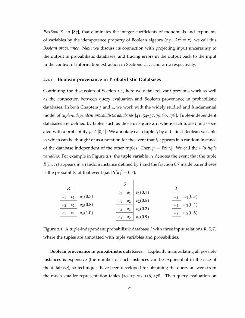
2.1.1 Boolean provenance in Probabilistic Databases

Continuing the discussion of Section 1.1, here we detail relevant previous work as well

as the connection between query evaluation and Boolean provenance in probabilistic

databases. In both Chapters 3 and 4, we work with the widely studied and fundamental

model of tuple-independent probabilistic databases [41, 54–57, 79, 86, 178]. Tuple-independent

databases are defined by tables such as those in Figure 2.1, where each tuple ti is associ-

ated with a probability pi ∈ [0,1]. We annotate each tuple ti by a distinct Boolean variable

ui which can be thought of as a notation for the event that ti appears in a random instance

of the database independent of the other tuples. Then pi = Pr[ui]. We call the ui’s tuple

variables. For example in Figure 2.1, the tuple variable u1 denotes the event that the tuple

R(b1, c1) appears in a random instance defined by I and the fraction 0.7 inside parentheses

is the probability of that event (i.e. Pr[u1] = 0.7).

R

b1 c1 u1(0.7)

b2 c2 u2(0.8)

b1 c3 u3(1.0)

S

c1 a1 v1(0.1)

c1 a2 v2(0.5)

c2 a3 v3(0.2)

c3 a2 v4(0.9)

T

a1 w1(0.3)

a2 w2(0.4)

a3 w3(0.6)

Figure 2.1: A tuple-independent probabilistic database I with three input relations R,S, T,

where the tuples are annotated with tuple variables and probabilities.

Boolean provenance in probabilistic databases. Explicitly manipulating all possible

instances is expensive (the number of such instances can be exponential in the size of

the database), so techniques have been developed for obtaining the query answers from

the much smaller representation tables [10, 17, 79, 116, 178]. Then query evaluation on

21

tuple-independent probabilistic databases reduces to the computation of probability of

the Boolean provenance of the output tuples given the probabilities of the source tuples

(see Section 1.1).

For all queries q, given a probabilistic database I, the computation of the probabilities

for the tuples in the answer q(I) can be presented in two stages [79, 178]. In the first stage

we compute the Boolean provenance for each tuple in the answer q(I). This first stage

is not a source of computational hardness, provided we are concerned, as is the case in

this dissertation, only with data complexity 10 (i.e., we assume that the size of the query is

a constant). Indeed, every Boolean provenance in q(I) is of polynomial size and can be

computed in polynomial time in the size of I.

q(x) : −R(x,y),S(y,z)

q(I)

b1 u1(v1 + v2) + u3v4

b2 u2v3

Figure 2.2: A safe query q and Boolean provenance of the output tuples in q(I).

In the second stage, the probability of each Boolean provenance is computed from the

probabilities that the model associates with the tuples in I, i.e., with the tuple variables

using the standard laws. For example, in Figure 2.2 the event that the output tuple b2

appears in q(I) for a random instance described by I is described by its Boolean prove-

nance u2v3. By the independence assumptions it has probability Pr[u2v3] = Pr[u2]Pr[v3] =

0.4× 0.2 = 0.08.

This break into two stages using the Boolean provenance is called intensional semantics

by Fuhr and Rolleke [79], and they observe that with this method computing the query

answer probabilities requires exponentially many steps in general. Indeed, the data com-

plexity of query evaluation on probabilistic databases is related to counting the number of

its satisfying assignments which leads to #SAT, Valiant’s first #P-complete problem [169],

This problem has shown to be #P-hard, even for conjunctive queries [86], in fact even for

quite simple Boolean queries like q() : −R(x),S(x,y), T(z) [55].

10In this dissertation, the data input consists of the representation tables [55, 86] (possible source tuples

and probabilities) rather than the collection of possible worlds.

22

Safe and Unsafe queries. Fuhr and Rolleke also observe that certain event inde-

pendences can be taken advantage of, when present, to compute answer probabilities in

PTIME, with a procedure called extensional semantics. The idea behind the extensional

approach is the starting point for the important dichotomy results of Dalvi et. al. [54–57].

In a series of seminal papers they showed that the positive queries can be decidably and

elegantly separated into those whose data complexity is #P-hard (called unsafe queries)

and those for whom a safe plan taking the extensional approach can be found to compute

the answer probabilities in poly-time (called safe queries). Figures 2.3 and 2.2 respectively

show examples of safe and unsafe queries.

q′(x) : −R(x,y),S(y,z), T(z)

q′(I)

b1 u1v1w1 + u1v2w2 + u3v4w2

b2 u2v3w3

Figure 2.3: An unsafe query q′ and Boolean provenance of the output tuples in q′(I).

However, even for safe queries the separate study of the Boolean provenance is bene-

ficial. Olteanu and Huang have shown that if a conjunctive query without self-join is safe

then for any database instance I the Boolean provenance of any output tuple in q(I) is

read-once [137]. A Boolean expression is in read-once form if each of its variables appears

exactly once, and is read-once if it is equivalent to a Boolean expression in read-once form.

It is easy to see that the probability of an expression whose variables denote independent

events can be computed in linear time if the expression is in read-once form (basic trick:

Pr[ϕ∨ ψ] = 1− (1− Pr[ϕ])(1− Pr[ψ]), because ϕ and ψ have disjoint sets of variables and

hence are independent). With hindsight, the quest in [55] for plans for safe queries that on

all inputs compute probability in poly-time can be seen as a quest for plans that compute

Boolean provenance directly in read-once form. In Figure 2.2, the Boolean provenance

of both the output tuples produced by the safe query q are already in read-once form,

and are computed in this form by the safe plan Πx(R 1 ΠyS) found through the algo-

rithm given in [55]. On the other hand, for the unsafe query q′ in Figure 2.3, the Boolean

provenance of the tuple q′(b1) is not read-once (there is no equivalent read-once form).

Using knowledge compilation techniques such as BDDs and d-DNNFs [60], the study of

23

Boolean provenance also enables poly-time computation of probabilities for classes of

queries larger than safe conjunctive queries without self-join [101, 137].

What of unsafe positive queries? As we saw from the example above, they can be quite

common and cannot be ignored. One observation relevant for both Chapters 3 and 4

is that an unsafe query q can produce Boolean provenance that are amenable to poly-

time computation on some instances of database. For instance, modify our example in

Figure 2.1 by deleting the tuple S(c3, a2). To obtain the modified Boolean provenance just

set the corresponding tuple variable v4 to 0 in Figure 2.3. The query q′ is unsafe, but on

this modified instance the Boolean provenance of the output tuple b1 is read-once because

u1v1w1 + u1v2w2 = u1(v1w1 + v2w2); therefore the efficient way of computing probabilities

applies. This leads to an “instance-by-instance” approach (discussed in Chapter 3, and

also in Chapter 4) that considers both query and the database instead of only classifying

the input query as safe or unsafe.

Another observation relevant for this dissertation is that giving up on the exact com-

putation of the probabilities solves the problem for unsafe positive queries. This is be-

cause the equivalent disjunctive normal form (DNF) of a Boolean provenance from a pos-

itive query is of polynomial size in the size of the database. Therefore, as shown in [55]

(see also [144]), an FPRAS (Fully Polynomial Randomized Approximation Scheme) can

be obtained by slightly adapting the well-known algorithm for DNF counting given by

Karp and Luby [104]. In this dissertation, however, for positive conjunctive queries with-

out self-join, we consider the problem of exactly evaluating the probabilities (Chapter 3).

On the other hand, for queries with difference operations, we focus on approximating

the probabilities (Chapter 4). Here we show that the exact computation is hard for very

simple queries, and there are queries for which even any non-trivial approximation may

not be possible. .

2.1.2 Boolean Provenance in Information Extraction

We discussed applications of Boolean provenance for source refinement in Section 1.1,

where it is used to trace uncertainty in the output back to the input. In Section 1.1,

we gave an example of view maintenance where a relational query is evaluated on an

24

input (relational) database to produce the output view. In this section we show another

interesting application of source refinement in information extraction, which can also be

abstracted using relational setting.

Information extraction systems aim to extract structured data like entities (e.g. Person,

Organization, Location) and relations between entities (e.g. Person’s birth date or phone

number) from unstructured text. The major components for most (rule-based) informa-

tion extraction systems are a set of dictionaries of entries (like names of people, organiza-

tion, location etc.) and a set of extraction rules. In Chapter 5, our goal is to improve the

quality of an information extraction system by refining the dictionaries used in the sys-

tem. Here we discuss the rule language, its abstraction using relational algebra operators,

and Boolean provenance of the output tuples in terms of the input dictionary entries. The

motivation behind dictionary refinement will be discussed in detail in Chapter 5.

match

t6: April Smith

match

t1: April

t2: Chelsea

t3: April

t4: Chelsea

text

t0: This April, mark your calendars for the last derby of the season: Arsenal at Chelsea. April Smith reporting live from Chelsea’s stadium.

Dictionary file first_names.dict: w1: chelsea, w2: john, w3: april… Dictionary file last_names.dict: w4: smith,… Dictionary file names.dict: w5: april smith, ,… R1: create view FirstName as Dictionary(‘first_names.dict’, Document, text); R2: create view LastName as Dictionary(‘last_names.dict’, Document, text); R3: create view FullName as Dictionary(‘names.dict’, Document, text);

R4: create view FirstLast as select Merge(F.match, L.match) as match from FirstName F, LastName L where FollowsTok(F.match, L.match, 0, 0);

R5: --Create the output of the extractor create table Person(match span);

insert into Person ( select * from FullName A ) union ( select * from FirstLast A ) union ( select * from FirstName A where Not(MatchesRegex(‘[ ]*[A-Z].*’, RightContextTok(A.match, 1))));

Input document: “This April, mark your calendars for the first derby of the season: Arsenal at Chelsea. April Smith reporting live from Chelsea’s stadium.”

Document:

FirstName: LastName: match

t5: Smith

FullName:

match

t8: April

t9: Chelsea

t10: April Smith

t11: Chelsea

Person:

match

t7: April Smith

FirstLast:

Figure 2.4: Example Person Extractor with Input Document, rules, dictionaries and inter-

mediate and output views.

Figure 2.4 illustrates a toy example of Person extractor. The inputs to an information

extraction system are a set of documents (“Input Document” in the figure), a set of dic-

tionaries (e.g. first names.dict, last names.dict, etc.), and a set of rules (R1 to R5). The output

25

is a set of extracted entities or relations (Person in the figure).

Rule Language: We use the SELECT - PROJECT - JOIN - UNION (SPJU) operations

from positive relational algebra queries. enriched with a number of basic extraction prim-

itives handling the input text. This subset expresses a core set of functionality underlying

most rule languages in common use today [12, 52, 114, 148, 157], and therefore our work

can be easily applied to the other rule languages. Specifically, we augment SQL with

some basic information extraction primitives like span, FollowsTok, Right(Left)ContextTok,

Merge and MatchesRegex. We explain these primitives using the example Person extractor

given in Figure 2.4.

To model data values extracted from the input document we add a new atomic data

type called span. A span is an ordered pair 〈begin, end〉 that identifies the region of an

input document between the begin and end offsets. We model the input document as

a table called Document with a single attribute of type span named text. For clarity, we

may sometimes identify a span using its string value and drop the offsets when they are

clear from the context. For example, to identify the region starting at offset 5 and ending

at offset 10 in the document in Figure 2.4 we may use 〈5,10〉, or 〈5,10〉: “April”, or simply,

“April”.

The extractor in Figure 2.4 consists of individual rules, labeled R1 through R5. Rules

R1 through R4 define logical views, while rule R5 materializes a table of extraction results.

In our subsequent discussion, we refer to tuples in the output of an extractor such as those

generated by R5 as output tuples, or extraction results, or simply occurrences, to distinguish

them from intermediate tuples, or intermediate results, generated by remaining extraction

rules (e.g., R1 to R4).

Rules R1, R2 and R3 illustrate one of our text extraction additions to SQL: the Dictio-

nary table function, which identifies all occurrences of a given set of terms specified as

entries in a dictionary file. The dictionary files used in R1 to R3 contain a list of common

first names, a list of common last names, and respectively a list of common full names.

The three rules define three single-column views FirstName, LastName and FullName con-

taining one intermediate tuple for each dictionary match in the document. Since each

dictionary entry may have multiple matches in a document, we use wi to denote individ-

26

ual dictionary entries in order to distinguish them from their matches in a document. For

example, the dictionary entry w1 generates the intermediate tuples t2 and t4.

Rule R4 identifies pairs of first and last names that are 0 tokens apart in the input

document. The view definition uses two of the scalar functions that we add to SQL: Fol-

lowsTok and Merge. The FollowsTok function is used as a JOIN predicate: it takes two spans

as arguments, along with a minimum and maximum character distance, and returns true

if the spans are within the specified distance of each other in the text. The Merge function

takes as input a pair of spans and returns the shortest span that completely covers both

input spans. (Merge is sensitive to the order of its input spans: if the second span appears

before the first, the result of is undefined.) The select clause of R4 uses Merge to define a

span that extends from the beginning of each first name to the end of the last name.

Finally, rule R5 materializes the table Person, which constitutes the output of our ex-

tractor. It uses a union clause to union together candidate name spans identified by rules

R3 and R4, as well as candidates identified by R1 that are not immediately followed by a

capitalized word. Note the where clause of the last union operand of R5 which uses two

other additions to SQL: the RightContextTok function returns the span of a given length

measured in tokens to the right of the input span, while the MatchesRegex predicate re-

turns true if the text of the input span matches the given regular expression. In this case,

the regular expression ‘[ ]*[A-Z].*’ identifies a sequence of zero or more whites-

paces, followed by an upper-case letter, followed by zero or more occurrences of any

character.

Provenance of the output tuples: In Chapter 5, our goal is to improve the quality

of an information extraction system by refining the noisy dictionaries used in the system.

Therefore, we model the dictionaries as input relations, where each entry in each dictio-

nary is annotated with a unique variable. The input text document is considered as a

trusted relation comprising the words, therefore, this relation is not annotated. Now to

relate to the notion of Boolean provenance, we assume a canonical algebraic representa-

tion of extraction rules as trees of operators. For the SPJU subset of the rule language,

the canonical representation is essentially the same as the representation of correspond-

ing SQL statements in terms of the relational operators. In addition, the other opera-

27

tions handling text are modeled as one of these relational operations. Extracting spans

from the text matching a dictionary entry (the Dictionary operation) is treated as SELECT,

whereas “merging” two spans combined by operators like FollowsTok is considered as

JOIN. Here we give an example. Prov(t10) = t6 + t7 = t6 + t3 · t5, since Prov(t7) = t3 · t5.

We regard individual dictionary entries as the source of intermediate tuples generated

by the Dictionary operator and express the provenance of an output tuple directly in

terms of the dictionary entries that are responsible for generating that output tuple. For

example, we have that Prov(t3) = w3, Prov(t5) = w4 and Prov(t6) = w5, and hence

Prov(t10) = w5 + w3 · w4.

2.2 Workflow Provenance

In this section, we discuss some preliminary notions of workflows and provenance in

workflows that will be used in Chapters 6 and 7. The coarse-grained workflow provenance

simply records the sequence of steps taken corresponding to the derivation of a dataset

as a whole [24, 62, 158]. This is unlike the fine-grained data provenance discussed in

the previous section, which considers derivation of each data item in a dataset from the

source data and captures all low level operations used in the derivation. Data prove-

nance has primarily been studied in the relational setting where the input and output

data values are stored as tuples in relational databases, or can be abstracted as relational

databases (see Section 2.1.1). However, in applications like scientific experiments, the sci-

entists need to handle more complex data than tuples (e.g.files) and more complicated

processes than relational algebra operations (e.g., algorithms in biological experiments).

Workflow provenance, that simply records the processes and data values involved in the

generation of a result, plays an important role in understanding and debugging scientific

experiments. Workflow provenance does not exhibit a well-defined semantics like data

provenance (e.g. equivalence under equivalent queries). Nevertheless, it facilitates under-

standing an experiment that uses complex data and processes by treating each data value

as a unit, and each process as a black-box.

In recent years, the importance of workflow provenance has been recognized by the

development of several influential workflow management systems, e.g., myGrid/Taverna

28

[136], Kepler [26], and VisTrails [78], that capture and store provenance in scientific work-

flows. A standard for provenance representation called the Open Provenance Model

(OPM) [129] has been designed, and is used in several of the aforementioned systems.

Similarly, for business processes, tools have been developed for tracking, capturing, and

processing large volumes of provenance data in order to monitor and analyze executions

of business operations [53, 153].

Abstracting the notion of workflows in the existing literature, in Section 2.2.1 we de-

scribe our workflow model as a graphical structure connecting nodes or modules by data

flow. Then in Section 2.2 we describe how provenance information of a set of executions

of the workflow can be stored using a provenance relation.

2.2.1 Workflows

A workflow comprises a set of processes, called modules, connected by edges indicating

potential data flow between modules. There are also initial input data to the workflow and

final output data from the workflow. Figure 2.5c shows an example workflow with three

modules m1,m2,m3. Here a1, a2 are initial inputs, a6, a7 are final output, and a3, a4, a5 are

intermediate data that connect the modules. Note that we allow data sharing, i.e., output

of a module can be fed as input to more than one modules. In Figure 2.5c, a4 is input to

both m2 and m3.

Note that the modules are connected in a DAG (Directed Acyclic Graph) structure in

Figure 2.5c11. This is the case under the assumption that the workflows are static and

all modules in the workflow are executed exactly once in any execution or run of the

workflow. In other words, the workflows do not involve any dynamic operations like

loops (repeated serial executions of a module), forks (repeated parallel executions of a

module), recursion, or decision processes (if-then-else). Although workflows may contain

these operations in practice, standard workflow repositories [2] show that most of the

real-life workflows have static structures. Moreover, static workflows form a simple and

fundamental, yet non-trivial class of workflows for publishing provenance information

while guaranteeing privacy.

11We can assume that all initial inputs originate from a dummy “source node” and all final outputs are

collected by a dummy “sink node” to complete the DAG structure.

29

2.2.2 Provenance Relations

In every execution of the workflow, given a set of initial data values, a set of data values

for intermediate and final data items are computed. We record the executions in a relation

with functional dependencies, that we call the provenance relation.

!"#

!$#

!%#

&%#

&'#

&(#

&$#

&"#

&)#&)#)#

&*#&&*#

I O

a1 a2 a3 a4 a5

0 0 0 1 1

0 1 1 1 0

1 0 1 1 0

1 1 1 0 1

(b) R1: Functionality of

m1 with functional depen-

dency a1a2→ a3a4a5

a1 a2 a3 a4 a5 a6 a7

0 0 0 1 1 1 0

0 1 1 1 0 0 1

1 0 1 1 0 0 1

1 1 1 0 1 1 1

(c) R: Provenance relation for work-

flow executions with functional de-

pendencies a1a2 → a3a4a5, a3a4 →

a6, and a4a5→ a7

Figure 2.5: An example workflow, and module and workflow executions as provenance

relations

Provenance Relations for Module Executions. We start with relation for a single mod-

ule, that constitutes a workflow with simplest possible structure and also serves as a

building block for a more complicated workflow. Let m be a module with a set I of input

data items and a set O of (computed) output data items. We model executions of m as

a relation R over a set of attributes A = I ∪O that satisfies the functional dependency

I → O. In other words, I serves as a (not necessarily minimal) key for R. We assume

that I ∩O = ∅, since each data item has a unique name. We will refer to I as the input

attributes of R and to O as its output attributes.

We assume that the values of each attribute a ∈ A come from a finite but arbitrarily

large domain ∆a, and let Dom = ∏a∈I ∆a and Range = ∏a∈O ∆a denote the domain and

range of the module m respectively. The relation R thus represents the (possibly partial)

function m : Dom→ Range and tuples in R describe executions of m, namely for every

t ∈ R, πO(t) = m(πI(t)). We overload the standard notation for projection, πA(R), and

30

use it for a tuple t ∈ R. Thus πA(t), for a set A of attributes, denotes the projection of t to

the attributes in A.

Example 2.1. Figure 2.5 shows a simple workflow involving three modules m1,m2,m3 with

Boolean input and output attributes; we will return to it shortly and focus for now on

the top module m1. Module m1 takes as input two data items, a1 and a2, and computes

a3=a1∨a2, a4=¬(a1∧a2) and a5=¬(a1⊕a2). (The symbol ⊕ denotes XOR). The relational

representation (functionality) of module m1 is shown in Figure 2.5b as relation R1, with

the functional dependency a1a2 −→ a3a4a5. For clarity, we have added I (input) and O

(output) above the attribute names to indicate their role.

Provenance Relations for Workflow Executions. A workflow W consists of a set of

modules m1, · · · ,mn, connected as a DAG (see, for instance, the workflow in Figure 2.5).

Each module mi has a set Ii of input attributes and a set Oi of output attributes. We

assume that (1) for each module, its input and output attributes are disjoint, i.e. Ii ∩Oi =

∅, (2) the output attributes of distinct modules are disjoint, namely Oi ∩Oj = ∅, for i 6= j

(since each data item is produced by a unique module), and (3) whenever an output

of a module mi is fed as input to a module mj the corresponding output and input

attributes of mi and mj are the same. The DAG shape of the workflow guarantees that

these requirements are not contradictory. Note that, it is possible that Ii ∩ Ij 6= ∅ for i 6= j

since we allow data sharing.

We model executions of W as a provenance relation R over the set of attributes A =

∪ni=1(Ii ∪Oi), satisfying the set of functional dependencies F = Ii→Oi : i ∈ [1,n]. Equiv-

alently, the provenance relation R for all possible executions of W can be formed by

joining the individual relations for the modules m1, · · · ,mn. Each tuple in R describes

an execution of the workflow W. In particular, for every t ∈ R, and every i ∈ [1,n],

πOi(t) = mi(πIi(t)).

Example 2.2. Returning to the sample workflow in Figure 2.5, let module m2 compute

a6 = a3⊕a4 and the module m3 compute a7 =¬(a4+a5). The relation R in Figure 2.5c

shows all possible executions of the workflow. The input and output attributes of modules

m1,m2,m3 respectively are (i) I1 = a1, a2, O1 = a3, a4, a5, (ii) I2 = a3, a4, O2 = a6 and

(iii) I3 = a4, a5, O3 = a7. The underlying functional dependencies in R reflect the keys

31

of the constituent modules, e.g. from m1 we have a1a2 −→ a3a4a5, from m2 we have

a3a4 −→ a6, and from m3 we have a4a5 −→ a7.

Note that since the modules in the workflow are static, the provenance relation R

contains the entire provenance information for any run of the workflow (all modules and

values of the other data items that have been used in the generation of an output data

item can be known). The preliminary notions related to module privacy will be discussed

in Chapters 6 and 7.

2.3 Complexity Classes and Approximation

In addition to the more standard notion of optimality, NP-hardness and polynomial

running time, we will use some other complexity classes, approximation algorithms, and

hardness of approximation in this dissertation.

In Chapter 3 and 4, we will frequently use the terms #P-hardness, FPRAS, and in-

approximability. The complexity class #P captures the class of function problems of the

form “compute f (x)”, where f is the number of accepting paths of a non-deterministic

turing machine. A problem is #P-hard if every problem in #P can be reduced to it by a

polynomial-time counting reduction. The canonical first #P-hard (also #P-complete) prob-

lem defined by Valiant is #SAT [169], which counts the number of satisfying assignments

of a Boolean formula.

An FPRAS (fully polynomial randomized approximation scheme) is a randomized algo-

rithm that runs in time polynomial in the input size and 1/ε (ε is the accuracy parameter)

and produces a result that is correct to within relative error (1 ± ε) with probability

≥ 3/4. The specific value of 3/4 is not important; the success probability can be boosted

to 1− δ for any given confidence parameter δ by repeating the experiment log(1/δ) times

and then taking the median of the values. On the other hand, a counting problem is

inapproximable, if it has no FPRAS under standard complexity assumptions.

We will use the following standard notions of approximation: an algorithm is said

to be a µ(n)-approximation algorithm for a given optimization problem, for some non-

decreasing function µ(n) : N+→ R+, if for every input of size n it outputs a solution of

value at most a multiplicative factor of µ(n) away from the optimum.

32

An optimization problem is said to be µ(n)-hard to approximate if a poly-time µ(n)-

approximation algorithm for the problem does not exist under standard complexity as-

sumptions. In Chapter 6, we will use standard complexity assumptions of the form

NP 6⊆ DTIME(n f (n)), where f (n) is a poly-logarithmic or sub-logarithmic function of n

and DTIME represents deterministic time. If a problem is Ω(µ(n))-hard to approximate

unless NP 6⊆ DTIME(n f (n)), then there cannot be a o(µ(n))-approximation algorithm

unless all problems in NP have O(n f (n))-time deterministic exact algorithms.

In Chapter 6, we also use APX-hardness. An optimization problem is said to be APX-

hard if there exists a constant ε > 0 such that a (1 + ε)-approximation in polynomial

time would imply P = NP. If a problem is APX-hard, then the problem cannot have

a PTAS, i.e, a (1 + ε)-approximation algorithm which runs in poly-time for all constant

ε > 0, unless P = NP. This chapter also discusses communication complexity of some

problems, which tries to quantify the amount of communication required to compute a

given function, ignoring the complexity of computation discussed so far.

33

Chapter 3

Query Evaluation in Probabilistic

Databases using Read-Once

Functions

In this chapter, we present our first work to efficiently compute the uncertainty in the

output from uncertain inputs. Here we evaluate probabilities of the output tuples in

probabilistic databases using read-once Boolean provenance (see Sections 1.1.1 and 2.1.1

for a discussion on the query evaluation in probabilistic databases).

3.1 Overview

For tuple-independent probabilistic databases, Dalvi and Suciu showed an elegant di-

chotomy result to divide the class of conjunctive queries into those whose data com-

plexity is #P-hard and those for whom a safe plan can be found to compute the answer

probabilities in poly-time [54–56]. Our starting point in this work is the observation that

even when the data complexity of a query is #P-hard (i.e. the query is unsafe [55]), there

may be classes of data inputs for which the computation can be done in poly-time. We

illustrate with a simple example.

Example 3.2. Consider the tuple-independent probabilistic database in Figure 3.1 and the

conjunctive query q() : −R(x),S(x,y), T(y). The Boolean provenance annotating the an-

34

R=

a1 w1(0.3)

b1 w2(0.4)

a2 w3(0.6)

S=

a1 c1 v1(0.1)

b1 c1 v2(0.5)

a2 c2 v3(0.2)

a2 d2 v4(0.1)

T=

c1 u1(0.7)

c2 u2(0.8)

d2 u3(0.4)

Figure 3.1: A tuple-independent probabilistic database where the tuples are annotated

with tuple variables and probabilities.

swer True is12

f = w1v1u1 + w2v2u1 + w3v3u2 + w3v4u3 (3.1)

This can be obtained with the standard plan π()((R ./ S) ./ T). However, it is equivalent

to

(w1v1 + w2v2)u1 + w3(v3u2 + v4u3) (3.2)

which has the property that each variable occurs exactly once.

The independence of source tuples allows us to use Pr(xy) = Pr(x)Pr(y) and Pr(x +

y) = 1− (1− Pr(x))(1− Pr(y)). Therefore, the probability of the answer (3.2) can be com-

puted as: P( f ) = P((w1v1 + w2v2)u1 + w3(v3u2 + v4u3))= 1− [1− P(w1v1 + w2v2)P(u1)]

[1− P(w3)P(v3u2 + v4u3)], where P(w1v1 +w2v2) = 1− [1− P(w1)P(v1)][1− P(w2)P(v2)]

and P(v3u2 + v4u3) = 1− [1− P(v3)P(u2)][1− P(v4)P(u3)].

It can be verified that there is no relational algebra plan that directly yields (3.2) above.

We can extend this example to an entire class of representation tables of unbounded size.

Boolean expressions where each variable appears exactly once have read-once forms, and

the expressions that are equivalent to read-once forms are called read-once13. Of course,

not all Boolean expressions are read-once, eg., xy + yz + zx or xy + yz + zu are not.

In this work, we consider only Boolean conjunctive queries. We can do this without

loss of generality because we can associate to a non-Boolean conjunctive query q and an

12To reduce the size of expressions and following established tradition we use + for ∨ and · for ∧, and we

even omit the latter in most terms.13Read-once expressions have been called by various names, eg., separable, fanout-free [95], repetition-

free [90], µ-expressions [170], non-repeating [141], but since the late 80’s [97] the terminology seems to have

converged on read-once

35

instance I a set of Boolean queries in the usual manner: for each tuple t in the answer

relation q(I), consider the Boolean conjunctive query Qt which is obtained from q by

replacing the head variables with the corresponding values in t. We will also use q(I) to

denote the Boolean expression generated by evaluating the query q on instance I, which

may have different (but equivalent) forms based on the query plan.

Moreover, we consider only queries without self-join. Therefore our queries have the

form q() : −R1(x1), . . . , Rk(xk) where R1, . . . , Rk are all distinct table names while the xi’s

are tuples of first order (FO) variables 14 or constants, possibly with repetitions, matching

the arities of the tables. If the database has tables that do not appear in the query, they

are of no interest, so we will always assume that our queries feature all the table names

in the database schema R.

Therefore the goal of the work is as follows: Given a tuple-independent database I and a

Boolean conjunctive query without self join q, when is q(I) read-once and if so, can its read-once

form be computed efficiently?

For this class of queries, we only need to work with monotone Boolean formulas (all

literals are positive, only disjunction and conjunction operations). Every such formula is

equivalent to (many) disjunctive normal forms (DNFs) which are disjunctions of conjunc-

tions of variables. These conjunctions are called implicants for the DNF. By idempotence

we can take the variables in an implicant to be distinct and the implicants of a DNF to

be distinct from each other. A prime implicant of a formula f is one with a minimal set of

variables among all that can appear in DNFs equivalent to f . By absorption, we can re-

tain only the prime implicants in a DNF. The result is called the irredundant DNF (IDNF)

of f , as it is uniquely determined by f (modulo associativity and commutativity). We

usually denote it by f IDNF. Note that in particular the set of prime implicants is uniquely

determined by f .

Golumbic et. al.[85] gave a fast algorithm to check read-onceness of a Boolean ex-

pression and compute the equivalent read-once form (if possible). However, the Boolean

expression has to be specified in IDNF. The algorithm is based upon a characterization in

14“First-order” is to emphasize the distinction between the variables in the query subgoals and the vari-

ables in the Boolean expressions.

36

terms of the formula’s co-occurrence graph by Gurvich [91] which we explain in Section 3.2.

However, for positive relational queries (even for conjunctive queries without self-join),

the size of the IDNF of Boolean provenance is polynomial in the size of the table, but often

(and necessarily) exponential in the size of the query. This is a good reason for avoiding

the explicit computation of the IDNFs, and in particular for not relying on the algorithm

in [85]. In a recent and independent work, Sen et al. [156] proved that for the Boolean

expressions that arise out of the evaluation of conjunctive queries without self-joins the

characterization in [91] can be simplified. However, it is also stated [156] that even

for conjunctive queries without self-joins computing co-occurrence graphs likely requires

obtaining the IDNF of the Boolean expressions.

In this context, we summarize our contributions in this chapter below.

1. We show that an excursion through the IDNF is in fact not necessary because the

co-occurrence graphs can be computed directly from the provenance graph [88, 105]

that captures the computation of the query on a table. Provenance graphs are DAG

representations of the Boolean provenance in such a way that most common subex-

pressions for the entire table (rather than just each tuple) are not replicated. The

smaller size of the provenance graphs likely provides practical speedups in the com-

putations (compared for example with the provenance trees of [156]). Moreover, our

approach may be applicable to other kinds of queries, as long as their provenance

graphs satisfy a simple criterion that we identify. To give more context to our re-

sults, we also note that Hellerstein and Karpinski[97] have shown that if RP 6= NP

then deciding whether an arbitrary monotone Boolean formula is read-once cannot

be done in PTIME in the size of the formula.

2. The restriction to conjunctive queries without self-joins further allows us to con-

tribute improvements even over an approach that composes our efficient compu-

tation of co-occurrence graphs with one of the linear-time algorithms to check the

desired property of these graphs [29, 49, 92]. Indeed, we show that only a certain

subgraph of the co-occurrence graph (we call it the co-table graph) is relevant for

our stated problem. The co-table graph can be asymptotically smaller than the co-

occurrence graph for some classes of queries and instances. To enable the use of

37

only part of the co-occurrence graph we contribute a novel algorithm that computes

(when they exist) the read-once forms, using two new ideas: row decomposition and

table decomposition. Using just connectivity tests (eg., DFS), our algorithm is simpler

to implement than the cograph recognition algorithms in [29, 49, 92] and it has the

potential of affecting the implementation of probabilistic databases.

The proof of completeness for our algorithm does not use the cograph characteriza-

tion on which [156] relies. As such, the algorithm itself provides an alternative new

characterization of read-once expressions generated by conjunctive queries without

self-joins. This may provide useful insights into extending the approach to handle

larger classes of queries. We compare the time complexity of our algorithm with

the previous approaches in detail.

It is also important to note that neither the results of this work, nor those of [156]

provide complexity dichotomies as does, eg. [55]. It is easy to give a family of probabilistic

databases for which the query in Figure 3.1 (c) generates event expressions of the form:

x1x2 + x2x3 + · · ·+ xn−1xn + xnxn+1. These formulas are not read-once, but with a simple

memoization (dynamic programming) technique we can compute their probability in time

linear in n (see Section A.1.1 in the appendix). In general, Jha and Suciu have studied

classes of queries that allow poly-time computation using other knowledge compilation

techniques beyond read-onceness of Boolean provenance[101].

Organization. In Section 3.2 we explain how to compute provenance DAGs for SELECT-

PROJECT-JOIN (SPJ) queries and compare the sizes of the co-occurrence and co-table

graphs. Section 3.3 presents a characterization of the co-occurrence graphs for conjunctive

queries without self-joins. The characterization uses the provenance DAG. With this char-

acterization we give an efficient algorithm for computing the co-table (and co-occurrence)

graph. In Section 3.4 we give an efficient algorithm that, using the co-table graph, checks

if the result of the query is read-once, and if so computes its read-once form. Putting to-

gether these two algorithms we obtain an efficient query-answering algorithm that is com-

plete for Boolean conjunctive queries without self-joins and tuple-independent databases

that yield read-once event expressions. In Section 3.5 we compare the time complexity of

this algorithm with that of Sen et al. [156], and other approaches that take advantage of

38

past work in the read-once and cograph literature. Related work, conclusions and ideas

for further work ensue.

3.2 Preliminaries

In this section we explain some notions that will be used later in this chapter.

3.2.1 Provenance Graphs

We start with provenance graphs (PG). The concept that we define here is a small variation

on the provenance graphs defined in [88, 105] where conjunctive queries (part of mapping

specifications) are treated as a black box. It is important for the provenance graphs used

in this work to reflect the structure of different SPJ query plans that compute the same

conjunctive query.

A provenance graph is a directed acyclic graph (DAG) H such that the nodes V(H) of

H are labeled by variables or by the operation symbols · and +. As we show below, each

node corresponds to a tuple in an event table that represents the set of possible worlds

of either the input database or some intermediate database computed by the query plan.

An edge u→ v is in E(H) if the tuple corresponding to u is computed using the tuple

corresponding to v in either a join (in which case u is labeled with ·) or a projection (in

which case u is labeled with +). The nodes with no outgoing edges are those labeled

with variables and are called leaves while the nodes with no incoming edges are called

roots (and can be labeled with either operation symbol). Provenance graphs (PGs) are

closely related to the lineage trees of [156]. In fact, the lineage trees are tree representations

of the Boolean event expressions, while PGs are more economical: they represent the

same expressions but without the multiplicity of common subexpressions. Thus, they are

associated with an entire table rather than with each tuple separately, each root of the

graph corresponding to a tuple in the table. 15

We explain how the SPJ algebra works on tables with PGs. If tables R1 and R2 have

PGs H1 and H2 then the PG for R1 ./ R2 is constructed as follows. Take the disjoint union

15Note that to facilitate the comparison with the lineage trees the edge direction here is the opposite of the

direction in [88, 105].

39

w3

v2

·

w2

· ·v4v3

w1

v1

·

Figure 3.2: Provenance graph for R ./ S.

·

w3

v1

·

w1

v2

w2

· ·v4v3

· · ·u2 u3u1

·

+

Figure 3.3: Provenance graph for π()((R ./ S) ./ T).

H of H1 and H2. For every t1 ∈ R1 and t2 ∈ R2 that do join, add a new root labeled with ·

and make the root of H1 corresponding to t1 and that of H2 corresponding to t2 children

of this new root. Afterwards, delete (recursively) any remaining roots from H1 and H2.

For example, referring again to Figure 3.1, the PG associated with the table computed by

R ./ S is shown in Figure 3.2.

For selection, delete (recursively) the roots that correspond to the tuples that do not

satisfy the selection predicate. For projection, consider a table T with PG H and X a

subset of its attributes. The PG for πXR is constructed as follows. For each t ∈ πXR, let

t1, . . . , tm be all the tuples in R that X-project to t. Add to H a new root labeled with + and

make the roots in H corresponding to t1, . . . , tm the children of this new root. Referring

again to Figure 3.1, the PG associated with the result of the query plan π()((R ./ S) ./ T)

is shown in Figure 3.3. Since the query is Boolean, this PG has just one root.

The Boolean provenance that annotate tuples in the event tables built in the inten-

sional approach can be read off the provenance graphs. Indeed, if t occurs in an (initial,

intermediate, or final) table T whose PG is H, then, starting at the root u of H corre-

sponding to t, traverse the subgraph induced by all the nodes reachable from u and

build the Boolean expression recursively using parent labels as operation symbols and

the subexpressions corresponding to the children as operands. For example, we read

(((w1 · v1) · u1) + (u1 · (w2 · v2)) + (u2 · (v3 ·w3)) + ((w3 · v4) · u3)) off the PG in Figure 3.3.

40

3.2.2 Co-occurrence Graphs vs. Co-table Graphs

Gurvich [91] gave a characterization of the read-once Boolean expressions in terms of

their co-occurrence graphs which is defined as follows:

Definition 3.3. The co-occurrence graph, notation Gco, of a Boolean formula f is an undirected

graph whose set of vertices V(Gco) is the set Var( f ) of variables of f and whose set E(Gco) of

edges is defined as follows: there is an edge between x and y iff they both occur in the same prime

implicant of f .

Therefore, Gco is uniquely determined by f and it can be constructed from f IDNF. This

construction is quadratic in the size of f IDNF but of course f IDNF can be exponentially

larger than f . Figure 3.4 shows the co-occurrence graph for the Boolean expression f in

equation (3.1) of Example 3.2. As this figure shows, the co-occurrence graphs for expres-

sions generated by conjunctive queries without self join are always k-partite16 graphs on

tuple variables from k different tables.

w1u1

w2

w3

u2

u3

v1

v4

v2

v3

Figure 3.4: Co-occurrence graph Gco for the Boolean provenance f in Example 3.2.

We are interested in the co-occurrence graph Gco of a Boolean formula f because it

plays a crucial role in f being read-once. [91] has shown that a monotone f is read-once

iff (1) it is “normal” and (2) its Gco is a “cograph”. We don’t need to discuss normality

because [156] has shown that for Boolean provenance that arise from conjunctive queries

without self-joins it follows from the cograph property. We will also avoid defining what

a cograph is (see [47, 49]) except to note that cograph recognition can be done in linear

time [29, 49, 92] and that when applied to the co-occurrence graph of f the recognition

16A graph (V1 ∪ · · · ∪Vk, E) is k-partite, if for any edge (u,v) ∈ E where u ∈ Vi and v ∈ Vj, i 6= j.

41

algorithms also produce, in effect, the read-once form of f , when it exists.

Although the co-occurrence graph of f is defined in terms of f IDNF, we show in

Section 3.3 that when f is the Boolean provenance produced by a Boolean conjunctive

query without self-joins then we can efficiently compute the Gco of f from the provenance

graph H of any plan for the query. Combining this with any of the cograph recognition

algorithms we just cited, this yields one algorithm for the goal of this work, which we

will call a cograph-help algorithm.

Because it uses the more general-purpose step of cograph recognition a cograph-help

algorithm will not fully take advantage of the restriction to conjunctive queries without

self-joins. Intuitively, with this restriction there may be lots of edges in Gco that are

irrelevant because they link tuples that are not joined by the query. This leads us to the

notion of co-table graph defined below.

Toward the definition of the co-table graph we also need that of table-adjacency graph,

denoted by GT, as follows:

Definition 3.4. Given a Boolean query without self-joins q() : −R1(x1), . . . , Rk(xk), the vertex

set V(GT) of its table-adjacency graph GT is the set of k table names R1, · · · , Rk. We will say

that Ri and Rj are adjacent iff xi and xj have at least one FO variable in common i.e., Ri and Rj

are joined by the query. The set of edges E(GT) consists of the pairs of adjacent table names.

R TS

Figure 3.5: Table-adjacency graph GT for the relations in Example 3.2.

The table-adjacency graph GT for the query in Example 3.2 is depicted in Figure 3.5.

This graph helps us remove edges irrelevant to a query from the graph Gco. For example,

if there is an edge between x ∈ Ri and x′ ∈ Rj in Gco, but there is no edge between Ri

and Rj in GT, then (i) either there is no path connecting Ri to Rj in GT (so all tuples in

Ri pair with all tuples in Rj), or, (ii) x and x′ are connected in Gco via a set of tuples

x1, · · · , x`, such that the tables containing these tuples are connected by a path in GT. Our

algorithm in Section 3.4 shows that all such edges (x, x′) can be safely deleted from Gco

for the evaluation of the query that yielded GT. Next we define a co-table graph.

42

w1u1

w2

w3

u2

u3

v1

v4

v2

v3

Figure 3.6: Co-table graph GC for the Boolean provenance f in Example 3.2.

Definition 3.5. The co-table graph GC is the subgraph of Gco with V(GC) = V(Gco) and such

that given two tuples x ∈ Ri and x′ ∈ Rj there is an edge (x, x′) ∈ E(GC) iff (x, x′) ∈ E(Gco) and

Ri and Rj are adjacent in GT.

Figure 3.6 shows the co-table graph GC generated by the example in Figure 3.1.

Co-occurrence graph vs. co-table graph. The advantage of using the co-table graph

instead of the co-occurrence graph is most dramatic in the following example:

Example 3.6. Consider q() :−R1(x1), R2(x2) where x1 and x2 have no common FO variable.

Assuming that each of the tables R1 and R2 has n tuples, Gco has n2 edges while GC has

none. A cograph-help algorithm must spend Ω(n2) time even if it only reads Gco.

On the other hand, GC can be as big as Gco. In fact, when GT is a complete graph (see

next example), GC = Gco.

Example 3.7. Consider q() : −R1(x1,y), . . . , Rk(xk,y) where xi and xj have no common FO

variable if i 6= j. Here GT is the complete graph on R1, . . . , Rk and GC = Gco.

However, it can be verified that both our algorithm and the cograph-help algorithm

have the same time complexity on the above example.

3.3 Computing the Co-Table Graph

In this section we show that given as input the provenance DAG H of a Boolean con-

junctive query plan without self-joins Q on a table-independent database representation

I, the co-table graph GC and the co-occurrence graph Gco of the Boolean formula Q(I)

(see definitions in section 3.2) can be computed in poly-time in the sizes of H, I and Q.

43

It turns out that GC and Gco are computed by similar algorithms, one being a minor

modification of the other. As discussed in section 3.1, the co-occurrence graph Gco can

then be used in conjunction with cograph recognition algorithms (eg., [29, 49, 92]), to find

the read-once form of Q(I) if it exists. On the other hand, the smaller co-table graph GC

is used by our algorithm described in section 3.4 for the same purpose.

We use Var( f ) to denote the sets of variables in a monotone Boolean expression f .

Recall that the provenance DAG H is a layered graph where every layer corresponds to

a select, project or join operation in the query plan. We define the width of H as the

maximum number of nodes at any layer of the DAG H and denote it by βH. The main

result in this section is summarized by the following theorem.

Theorem 3.8. Let f = Q(I) be the Boolean expression computed by the query plan Q on the table

representation I ( f can also be read off the provenance graph of Q on I, H), n = |Var( f )| be the

number of variables in f , mH = |E(H)| be the number of edges of H, βH be the width of H, and

mco = |E(Gco)| be the number of edges of Gco, the co-occurrence graph of f .

1. Gco can be computed in time O(nmH + βHmco).

2. Further, the co-table graph GC of f can be computed in time O(nmH + βHmco + k2α logα)

where k is the number of tables in Q, and α is the maximum arity (width) of the tables in Q.

3.3.1 LCA-Based Characterization of the Co- Occurrence Graph

Here we give a characterization of the presence of an edge (x,y) in Gco based on the least

common ancestors of x and y in the graph H.

Again, let f = Q(I) be the Boolean expression computed by the query plan Q on the

table representation I. As explained in section 3.2 f can also be read off the provenance

graph H of Q and I since H is the representation of f without duplication of common

subexpressions.

The absence of self-joins in Q implies the following.

Lemma 3.9. The DNF generated by expanding f (or H) using only the distributivity rule is in

fact the IDNF of f up to idempotency (i.e. repetition of the same prime implicant is allowed).

44

Proof. Let g be the DNF generated from f by applying distributivity repeatedly. Due to

the absence of self-joins g every implicant in g will have exactly one tuple from every

table. Therefore, for any two implicants in g the set of variables in one is not a strict

subset of the set of variables in the other and further absorption (eg., xy + xyz = xy) does

not apply. (At worst, two implicants can be the same and the idempotence rule reduces

one.) Therefore, g is also irredundant and hence the IDNF of f (up to commutativity and

associativity).

Denote by f IDNF the IDNF of f , which, as we have seen, can be computed from f just

by applying distributivity.

As with any DAG, we can talk about the nodes of H in terms of successors, prede-

cessors, ancestors, and descendants, and finally about the least common ancestors of two

nodes, denoted lca(x,y). Because H has a root lca(x,y) is never empty. When H is a

tree, lca(x,y) consists of a single node. For a node u ∈ V(H), we denote the set of leaf

variables which are descendants of u by Var(u) (overloaded notation warning!); in other

words, a variable x belongs to Var(u), u ∈ V(H), if and only if x is reachable from u in

H. Now we prove the key lemma of this section:

Lemma 3.10. Two variables x,y ∈ Var( f ) belong together to a (prime) implicant of f IDNF if and

only if the set lca(x,y) contains a ·-node.

Proof. (if) Suppose lca(x,y) contains a ·-node u, i.e., x,y are both descendants of two

distinct successors v1,v2 of u. Since the · operation multiplies all variables in Var(v1)

with all variables in Var(v2), x and y will appear together in some implicant in f IDNF

which will not be absorbed by other implicants by Lemma 3.9.

(only if) Suppose that x,y appear together in an implicant of f IDNF and lca(x,y)

contains no ·-node. Then no ·-node in V(H) has x,y in Var(v1),Var(v2), where v1,v2 are

its two distinct successors (note that any ·-node in a provenance DAG H can have exactly

two successors). This implies that x and y can never be multiplied, contradiction.

Since there are exactly k tables in the query plan, every implicant in f IDNF will be of

size k. Therefore:

45

Lemma 3.11. For every variable x ∈ Var( f ) and ·-node u ∈ V(H), if x ∈ Var(u), then x ∈

Var(v) for exactly one successor v of u.

Proof. If x ∈ Var( f ) belongs to Var(v1),Var(v2) for two distinct successors v1,v2 of u,

then some implicant in f IDNF will have < k variables since x · x = x by idempotence.

The statement of Lemma 3.10 provides a criterion for computing Gco using the compu-

tation of least common ancestors in the provenance graph, which is in often more efficient

than computing the entire IDNF. We have shown that this criterion is satisfied in the case

of conjunctive queries without self-joins. But it may also be satisfied by other kinds of

queries, which opens a path to identifying other cases in which such an approach would

work.

3.3.2 Computing the Table-Adjacency Graph

It is easier to describe the computation of GT if we use the query in rule form Q() :

−R1(x1), . . . , Rk(xk).

The rule form can be computed in linear time from the SPJ query plan. Now the vertex

set V(GT) is the set of table names R1, · · · , Rk. and an edge exists between Ri, Rj iff xi and

xj have at least one FO variable in common i.e., Ri and Rj are joined. Whether or not such

an edge should be added can be decided in time O(α logα) by sorting and intersecting xi

and xj. Here α is the maximum arity (width) of the tables R1, · · · , Rk. Hence GT can be

computed in time O(k2α logα).

3.3.3 Computing the Co-Table Graph

Recall that co-table graph GC is a subgraph of the co-occurrence graph Gco where we

add an edge between two variables x,y, only if the tables containing these two tuples

are adjacent in the table-adjacency graph GT. Algorithm 1 CompCoTable constructs the

co-table graph GC by a single bottom-up pass over the graph H.

It is easy to see that a minor modification of the same algorithm can be used to

compute the co-occurrence graph Gco: in Step 11 we simply skip the check whether the

tables containing the two tuples are adjacent in GT. Since this is the only place where

46

Algorithm 1 Algorithm CompCoTable

Input: Query plan DAG H and table-adjacency graph GT

Output: Co-table graph GC.

1: – Initialize V(GC) = Var( f ), E(GC) = φ.

2: – For all variables x ∈ Var( f ), set Var(x) = x.

3: – Do a topological sort on H and reverse the sorted order.

4: for every node u ∈ V(H) in this order do

5: /* Update Var(u) set for both +-node and ·-node u*/

6: – Set Var(u) =⋃

vVar(v), where the union is over all successors v of u.

7: if u ∈ V(H) is a ·-node then

8: /* Add edges to GC only for a ·-node*/

9: – Let v1,v2 be its two successors.

10: for every two variables x ∈ Var(v1) and y ∈ Var(v2) do

11: if (i) the tables containing x,y are adjacent in GT and (ii) the edge (x,y) does

not exist in E(GC) yet then

12: – Add an edge between x and y in E(GC).

13: end if

14: end for

15: end if

16: end for

GT is used, the time for the computation of GC does not include the time related to

computing/checking GT.

Correctness. By a simple induction, it can be shown that the set Var(u) is correctly

computed at every step, i.e., it contains the set of all nodes which are reachable from u

in H (since the nodes are processed in reverse topological order and Var(u) is union of

Var(v) for over all successors v of u). Next lemma shows that algorithm CompCoTable

correctly builds the co-table graph GC (proof is in Appendix A.1.2).

Lemma 3.12. Algorithm CompCoTable adds an edge (x,y) to GC if and only if x,y together

appear in some implicant in f IDNF and the tables containing x,y are adjacent in GT.

Time Complexity. Here we give a sketch of the time complexity analysis, details

47

can be found in the appendix (Section A.1.3). Computation of the table adjacency graph

takes O(k2α logα) time as shown in Section 3.3.2. The total time complexity of algorithm

CompCoTable as given in Theorem 3.8 is mainly due to two operations: (i) computation

of the Var(u) set at every internal node u ∈ V(H), and (ii) to perform the test for pairs

x,y at two distinct children of a ·-node, whether the edge (x,y) already exists in GC, and

if not, to add the edge.

We show that the total time needed for the first operation is O(nmH) in total: for

every internal node u ∈V(H) we can scan the variables sets of all its immediate successor

in O(ndu) time to compute Var(u), where du is the outdegree of node u in H. This

gives total O(nmH) time. On the other hand, for adding edges (x,y) in GC, it takes total

O(mcoβH) time during the execution of the algorithm, where mco is the number of edges

in the co-occurrence graph (and not in the co-table graph, even if we compute the co-table

graph GC) and βH is the width of the graph H. To show this, we show that two variables

x,y are considered by the algorithm at Step 10 if and only if the edge (x,y) already exists

in the co-occurrence graph Gco, however, the edge may not be added to the co-table graph

GC if the corresponding tables are not adjacent in the table adjacency graph GT. We also

show that any such edge (x,y) will be considered at a unique level of the DAG H. In

addition to these operations, the algorithm does initialization and a topological sort on

the vertices which take O(mH + nH) time (nH = |V(H)|) and are dominated by the these

two operations.

3.4 Computing the Read-Once Form

Our algorithm CompRO (for Compute Read-Once) takes an instance I of the schema R =

R1, · · · , Rk, a query Q() :−R1(x1), R2(x2), · · · , Rk(xk) along with the table adjacency graph

GT and co-table graph GC computed in the previous section as input, and outputs whether

Q(I) is read-once. (if so it computes its unique read-once form).

Theorem 3.13. Suppose we are given a query Q, a table-independent database representation I,

the co-table graph GC and the table-adjacency graph GT for Q on I as inputs. Then

1. Algorithm CompRO decides correctly whether the expression generated by evaluating Q on

48

I is read-once, and if yes, it returns the unique read-once form of the expression, and,

2. Algorithm CompRO runs in time O(mTα logα + (mC + n)min(k,√

n)),

where mT = |E(GT)| is the number of edges in GT, mC = |E(GC)| is the number of edges in GC,

n is the total number of tuples in I, k is the number of tables, and α is the maximum size of any

subgoal.

3.4.1 Algorithm CompRO

In addition to the probabilistic database with tables R1, · · · , Rk and input query Q, our

algorithm also takes the table-adjacency graph GT and the co-table graph GC computed in

the first phase as discussed in Section 3.3. The co-table graph GC also helps us to remove

unused tuples from all the tables which do not appear in the final expression – every

unused tuple won’t have a corresponding node in GC. So from now on we can assume

wlog. that every tuple in every table appears in the final expression f .

The algorithm CompRO uses two decomposition operations: Row decomposition is a

horizontal decomposition operation which partitions the rows or tuples in every table into

the same number of groups and forms a set of sub-tables from every table. On the other

hand, Table decomposition is a vertical decomposition operation. It partitions the set of

tables into groups and a modified sub-query is evaluated in every group. For convenience,

we will represent the instance I as R1[T1], · · · , Rk[Tk], where Ti is the set of tuples in table

Ri. Similarly, for a subset of tuples T′i ⊆ Ti, Ri[T′i ] will denote the instance of relation Ri

containing exactly the tuples in T′i . The algorithm CompRO is given in Algorithm 2.

Row Decomposition. The row decomposition operation partitions the tuples variables

in every table into ` disjoint groups. In addition, it decomposes the co-table graph GC into

` ≥ 2 disjoint induced subgraphs17 corresponding to the above groups. For every pair of

distinct groups j, j′, and for every pair of distinct tables Ri, Ri′ , no tuple in group j of Ri

ever joins with a tuple in group j′ of Ri′ (recall that the query does not have any self-join

operation). The procedure for row decomposition is given in Algorithm 3. It should be

17A subgraph H of G is an induced subgraph, if for any two vertices u,v ∈ V(H), if (u,v) ∈ E(G), then

(u,v) ∈ E(H).

49

Algorithm 2 CompRO(Q, I = 〈R1[T1], · · · , Rk[Tk]〉, GC, GT, Flag)Input: Query Q, tables R1[T1], · · · , Rk[Tk], co-table graph GC, table-adjacency graph GT,

and a Boolean parameter Flag which is true if and only if row decomposition is per-

formed at the current step.

Output: If successful, the unique read-once form f ∗ of the expression for Q(I)

1: if k = 1 then

2: return ∑x∈T1x with success. (/* all unused tuples are already removed */)

3: end if

4: if Flag = True then /* Row decomposition */

5: – Perform RD(〈R1[T1], · · · , Rk[Tk]〉, GC).

6: if row decomposition returns with success then /* RD partitions every table and GC

into ` ≥ 2 disjoint groups*/

7: – Let the groups returned be 〈〈T j1, · · · , T j

k〉, GC,j〉, j ∈ [1,`].

8: – ∀j ∈ [1,`], let f j = CompRO(Q, 〈R1[Tj1], · · · , Rk[T

jk]〉, GC,j, GT,False).

9: return f ∗ = f1 + · · ·+ f` with success.

10: end if

11: else /* Table decomposition */

12: – Perform TD(〈R1[T1], · · · , Rk[Tk]〉, Q, GT, GC).

13: if table decomposition returns with success then /* TD partitions I, GC and GT into

` ≥ 2 disjoint groups, ∑`j=1 k j = k */

14: Let the groups returned be 〈〈Rj,1, · · · , Rj,k j〉, Qj, GC,j, GT,j〉, j ∈ [1,`].

15: – ∀j ∈ [1,`], f j = CompRO(Qj, 〈R1[T1], · · · , Rk[Tk]〉, GC,j, GT,j,True).

16: return f ∗ = f1 · . . . · f` with success.

17: end if

18: end if

19: if the current operation is not successful then /* Current row or table decomposition is

not successful and k > 1*/

20: return with failure: “Q(I) is not read-once”.

21: end if

50

noted that the row decomposition procedure may be called on Ri1 [T′i1 ], · · · , Rip [T

′ip] and G′C,

where Ri1 , · · · , Rip is a subset of the relations from R1, · · · , Rk, T′i1 , · · · , T′ipare subsets of the

respective set of tuples Ti1 , · · · , Tip , and G′C is the induced subgraph of GC on T′i1 , · · · , T′ip.

For simplicity in notations, we use R1[T1], · · · , Rk[Tk]. This holds for table decomposition

as well.

Algorithm 3 RD(〈R1[T1], · · · , Rk[Tk]〉, G′C)

Input: Tables R1[T1], · · · , Rk[Tk], and induced subgraph G′C of GC on⋃k

i=1 Ti

Output: If successful, the partition of G′C and tuple variables of every input tables into

` ≥ 2 connected components: 〈〈T1,j, · · · , Tk,j〉, G′C,j〉, j ∈ [1,`]

1: – Run BFS or DFS to find the connected components in G′C.

2: – Let ` be the number of connected components.

3: if ` = 1 then /* there is only one connected component */

4: return with failure: “Row decomposition is not possible”.

5: else

6: – Let the tuples (vertices) of table Ri in the j-th connected component j of G′C be Ti,j

7: – Let the induced subgraph for connected component j be GC,j.

8: return 〈〈T1,1, · · · , Tk,1〉, G′C,1〉, · · · , 〈〈T1,`, · · · , Tk,`〉, G′C,`〉 with success.

9: end if

Table Decomposition. On the other hand, the table decomposition operation partitions

the set of tables R = R1, · · · , Rk into ` ≥ 2 disjoint groups R1, · · · ,R`. It also decomposes

the table-adjacency graph GT and co-table graph GC into ` disjoint induced subgraphs

GT,1, · · · , GT,`, and, GC,1, · · · , GC,` respectively corresponding to the above groups. The

groups are selected in such a way that all tuples in the tables in one group join with

all tuples in the tables in another group. This procedure also modifies the sub-query

to be evaluated on every group by making the subqueries of different groups mutually

independent by introducing free variables, i.e., they do not share any common variables

after a successful table decomposition. Algorithm 4 describes the table decomposition

operation. Since the table decomposition procedure changes the input query Q to Q =

Q1, · · · , Q`, it is crucial to ensure that changing the query to be evaluated does not change

51

the answer to the final expression (see Lemma A.5 in Appendix A.1.4).

The following lemma shows that if row-decomposition is successful, then table decom-

position cannot be successful and vice versa. However, both of them may be unsuccessful

when the Boolean provenance is not read-once (proof is in Appendix A.1.4).

Lemma 3.14. At any step of the recursion, if row decomposition is successful then table decom-

position is unsuccessful and vice versa.

Therefore, in the top-most level of the recursive procedure, we can verify which oper-

ation can be performed – if both of them fail, then the final expression is not read-once

which follows from the correctness of our algorithm. If the top-most recursive call per-

forms a successful row decomposition initially the algorithm CompRO is called as Com-

pRO(Q, 〈R1[T1], · · · , Rk[Tk]〉, GC, GT, True). The last Boolean argument is True if and only

if row decomposition is performed at the current level of the recursion tree. If in the first

step table decomposition is successful, then the value of the last Boolean variable in the

initial call will be False.

Correctness. The following two lemmas respectively show the soundness and com-

pleteness of the algorithm CompRO (proofs are in Appendix A.1.4).

Lemma 3.15. (Soundness) If the algorithm returns with success, then the expression f ∗ returned

by the algorithm CompRO is equivalent to the expression Q(I) generated by evaluation of query

Q on instance I. Further, the output expression f ∗ is in read-once form.

Lemma 3.16. (Completeness) If the expression Q(I) is read-once, then the algorithm CompRO

returns the unique read-once form f ∗ of the expression.

For completeness, it suffices to show that if Q(I) is read-once, then the algorithm

does not exit with error. Indeed, if the algorithm returns with success, as showed in the

soundness lemma, the algorithm returns an expression f ∗ in read-once form which is the

unique read-once form of Q(I) [85],[47].

Time Complexity. Consider the recursion tree of the algorithm CompRO. Lemma 3.14

shows that at any level of the recursion tree, either all recursive calls use the row decom-

position procedure, or all recursive calls use the column decomposition procedure. The

time complexity of CompRO given in Theorem 3.13 is analyzed in the following steps. If

52

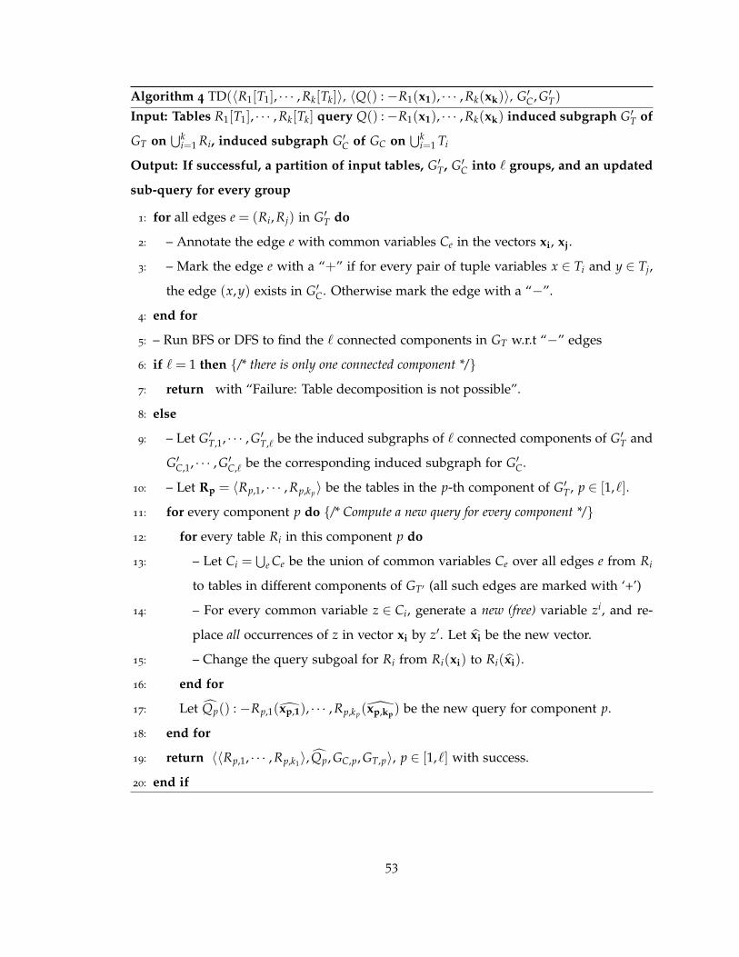
Algorithm 4 TD(〈R1[T1], · · · , Rk[Tk]〉, 〈Q() : −R1(x1), · · · , Rk(xk)〉, G′C, G′T)Input: Tables R1[T1], · · · , Rk[Tk] query Q() :−R1(x1), · · · , Rk(xk) induced subgraph G′T of

GT on⋃k

i=1 Ri, induced subgraph G′C of GC on⋃k

i=1 Ti

Output: If successful, a partition of input tables, G′T, G′C into ` groups, and an updated

sub-query for every group

1: for all edges e = (Ri, Rj) in G′T do

2: – Annotate the edge e with common variables Ce in the vectors xi, xj.

3: – Mark the edge e with a “+” if for every pair of tuple variables x ∈ Ti and y ∈ Tj,

the edge (x,y) exists in G′C. Otherwise mark the edge with a “−”.

4: end for

5: – Run BFS or DFS to find the ` connected components in GT w.r.t “−” edges

6: if ` = 1 then /* there is only one connected component */

7: return with “Failure: Table decomposition is not possible”.

8: else

9: – Let G′T,1, · · · , G′T,` be the induced subgraphs of ` connected components of G′T and

G′C,1, · · · , G′C,` be the corresponding induced subgraph for G′C.

10: – Let Rp = 〈Rp,1, · · · , Rp,kp〉 be the tables in the p-th component of G′T, p ∈ [1,`].

11: for every component p do /* Compute a new query for every component */

12: for every table Ri in this component p do

13: – Let Ci =⋃

e Ce be the union of common variables Ce over all edges e from Ri

to tables in different components of GT′ (all such edges are marked with ‘+’)

14: – For every common variable z ∈ Ci, generate a new (free) variable zi, and re-

place all occurrences of z in vector xi by z′. Let xi be the new vector.

15: – Change the query subgoal for Ri from Ri(xi) to Ri(xi).

16: end for

17: Let Qp() : −Rp,1(xp,1), · · · , Rp,kp(xp,kp) be the new query for component p.

18: end for

19: return 〈〈Rp,1, · · · , Rp,k1〉, Qp, GC,p, GT,p〉, p ∈ [1,`] with success.

20: end if

53

n′ = the total number of input tuples at the current recursive call and m′C = the number

of edges in the induced subgraph of G′C on these n′ vertices, we show that row decom-

position takes O(m′C + n′) time and, not considering the time needed to compute the modified

queries Qj (Step 11 in Algorithm 4), the table decompositions procedure takes O(m′C + n′)

time. Then we consider the time needed to compute the modified queries and show

that these steps over all recursive calls of the algorithm take O(mTα logα) time in total,

where α is the maximum size of a subgoal in the query Q. Finally, we give a bound of

O(min(k,√

n)) on the height of the recursive tree for the algorithm CompRO. However,

note that at every step, for row or table decomposition, every tuple in G′C goes to exactly

one of the recursive calls, and every edge in G′C goes to at most one of the recursive calls.

So for both row and table decomposition at every level of the recursion tree the total time

is O(mC + n). Combining all these observations, the total time complexity of the algo-

rithm is O(mTα logα + (mC + n)min(k,√

n)) as stated in Theorem 3.13. The details can

be found in Appendix A.1.5.

Example. Here we illustrate our algorithm. Consider the query Q and instance I

from Example 3.2 in the introduction. The input query is Q() : −R(x)S(x,y)T(y). In the

first phase, the table-adjacency graph GT and the co-table graph GC are computed. These

graphs are depicted in Fig. 3.5 and Fig. 3.6 respectively.

Now we apply CompRO. There is a successful row decomposition at the top-most

recursive call that decomposes GC into the two subgraphs GC,1, GC,2 shown in Fig. 3.7.

So the final expression f ∗ annotating the answer Q(I) will be the sum of the expressions

f1, f2 annotating the answers of Q applied to the relations corresponding to GC,1 and GC,2

respectively.

w1

w2

v1

v2

u1 w3

u2

u3

v3

v4

Figure 3.7: GC,1 and GC,2.

The relations corresponding to GC,1 are

R =a1 w1

b1 w2

S =a1 c1 v1

b1 c1 v2

T = c1 u1

54

and, the relations corresponding to GC,2 are

R = a2 w3 S =a2 c2 v3

a2 d2 v4

T =c2 u2

d2 u3

Now we focus on the first recursive call at the second level of recursion tree with

input co-table subgraph GC,1. Note that the table-adjacency graph for this call is the same

as GT. At this level the table decomposition procedure is invoked and the edges of the

table-adjacency graph are marked with + and − signs, see Fig. 3.8. In this figure the

common variable set for R,S on the edge (R,S) is x, and for S, T on the edge (S, T) is

y. Further, the edge (S, T) is marked with a “+” because there are all possible edges

between the tuples in S (in this case tuples v1,v2) and the tuples in T (in this case u1).

However, tuples in R (here w1,w2) and tuples in S (here v1,v2) do not have all possible

edges between them so the edge (R,S) is marked with a “−”.

Table decomposition procedure performs a connected component decomposition us-

ing “−”-edges, that decomposes GT in two components R,S and T. The subset C

of common variables collected from the “+”-edges across different components will be

the variables on the single edge (S, T), C = y. This variable y is replaced by new

free variables in all subgoals containing it, which are S and T in our case. So the modi-

fied queries for disjoint components returned by the table decomposition procedure are

Q1() :−R(x)S(x,y1) and Q2() :−T(y2). The input graph GC,1 is decomposed further into

GC,1,1 and GC,1,2, where GC,1,1 will have the edges (w1,v1) and (w2,v2), whereas GC,1,2

will have no edges and a single vertex u1. Moreover, the expression f1 is the product of

f11 and f12 generated by these two queries respectively. Since the number of tables for

Q2 is only one, and T has a single tuple, by the base step (Step 2) of CompRO, f12 = u1.

For expression f11 from Q1, now the graph GC,1,1 can be decomposed using a row de-

composition to two connected components with single edges each ((w1,v1) and (w2,v2)

respectively). There will be recursive subcalls on these two components and each one of

them will perform a table decomposition (one tuple in every table, so the single edges in

both calls will be marked with “+”). Hence f11 will be evaluated to f11 = w1v1 + w2v2. So

f1 = f11 · f12 = (w1v1 + w2v2)u1.

By a similar analysis as above, it can be shown that the same query Q evaluated on the

55

R S T−, x +,y

Figure 3.8: Marked table-adjacency graph for R,S, T.

tables R,S, T given in the above tables give f2 = w3(v3v4 + u2u3). So the overall algorithm

is successful and outputs the read-once form f ∗ = f1 + f2 = (w1v1 + w2v2)u1 + w3(v3u2 +

v4u3).

3.5 Discussion

To evaluate our approach, we discuss the time complexity of the entire query-answering

algorithm and compare it with the time complexity of the previous algorithms. Putting

together our results from Sections 3.3 and 3.4, we propose the following algorithm for an-

swering Boolean conjunctive queries without self-joins on tuple-independent probabilistic

databases.

• Phase 0 (Compute provenance DAG)

Input: query q, event table rep I

Output: provenance DAG H

Complexity: O(( nek )

k) (see below)

• Phase 1 (Compute co-table graph)

Input: H, q

Output: table-adjacency graph GT, co-table graph GC

Complexity: O(nmH + βHmco + k2α logα) (Thm. 3.8)

• Phase 2 (Compute read-once form)

Input: event table rep I, q, GT, GC

Output: read-once form f ∗ or FAIL

Complexity: O(mTα logα + (mC + n)min(k,√

n)) (Thm. 3.13)

Size of the provenance DAG H. Let f be the Boolean provenance generated by some

query plan for q on the database I. The number of edges mH in the DAG H represents

56

the size of the expression f . Since there are exactly k subgoals in the input query q, one

for every table, every prime implicant of f IDNF will have exactly k variables, so the size of

f IDNF is at most (nk)≤ ( ne

k )k. Further, the size of the input expression f is maximum when

f is already in IDNF. So size of the DAG H is upper bounded by mH ≤ ( nek )

k. Again, the

“leaves” of the DAG H are exactly the n variables in f . So mH ≥ n− 1, where the lower

bound is achieved when the DAG H is a tree (every node in H has a unique predecessor);

in that case f must be read-once and H is the unique read-once tree of f .

Therefore n − 1 ≤ mH ≤ ( nek )

k. Although the upper bound is quite high, it is our

contention that for practical query plans the size of the provenance graph is much smaller

than the size of the corresponding IDNF.

Data complexity. The complexity dichotomy of [55] is for data complexity, i.e., the

size of the query is bounded by a constant. This means that our k and α are O(1). Hence

the time complexities of the Phase 1 and Phase 2 are O(nmH + βHmco) and O(mC + n)

respectively. Since the co-occurrence graph is at least as large as the co-table graph mco ≥

mC, and therefore the first phase always dominates asymptotically.

In any case, we take the same position as [156] that for unsafe queries [55] the com-

petition comes from the approach that does not try to detect whether the formulas are

read-once and instead uses probabilistic inference [111] which is in general EXPTIME. In

contrast, our algorithm runs in PTIME, and works for a larger class of queries than the

safe queries [55] (but of course, not on all instances).

Comparisons with other algorithms. Here we do not restrict ourselves to data com-

plexity, instead taking the various parameters of the problem into consideration.

First consider the general read-once detection algorithm. This consists of choosing

some plan for the query, computing the answer Boolean provenance f , computing its

IDNF, and then using the (so far, best) algorithm [85] to check if f is read-once and if

so to compute its read-once form. The problem with this approach is that the read-once

check is indeed done in time a low polynomial, but in the size of f IDNF. For example,

consider a Boolean query like the one in Example 3.6. This is a query that admits a plan

(the safe plan!) that would generate the Boolean provenance (x1 + y1) · · · (xn + yn) on an

instance in which each Ri has two tuples xi and yi. This is a read-once expression easily

57

detected by our algorithm, which avoids the computation of the IDNF.

Next consider the cograph-help algorithm that we have already mentioned and jus-

tified in Section 3.2. This consists of our Phase 0 and a slightly modified Phase 1 that

computes the co-occurrence graph Gco, followed by checking if Gco is a cograph using one

of the linear-time algorithms given in [29, 49, 92] which also outputs the read-once form

if possible. Since Phase 0 and Phase 1 are common we only need to compare the last

phases.

The co-graph recognition algorithms will all run in time O(mco + n). Our Phase 2

complexity is better than this when mC min(k,√

n) = o(mco) (for instance, when we con-

sider data complexity assuming that the query size is much smaller than the size of the

data). Although in the worst case this algorithm performs at least as well as our algorithm

(when mC is θ(mco) and we consider combined complexity including both the data and

the query size), (i) almost always the query will be of much smaller size than the data,

and therefore the time required in first phases will dominate, so the asymptotic running

time of both these algorithms will be comparable, (ii) as we have shown earlier, the ratiomcomC

can be as large as Ω(n2), and the benefit of this could be significantly exploited by

caching co-table graphs computed for other queries (see discussions in Section 3.7), and

(iii) these linear time algorithms use complicated data structures, whereas we use simple

graphs given as adjacency lists and connectivity-based algorithms, so our algorithms are

simpler to implement and may run faster in practice.

Finally we compare our algorithm against that given in [156]. Let us call it the lineage-

tree algorithm since they take the lineage tree of the result as input as opposed to the

provenance DAG as we do. Although [156] does not give a complete running time anal-

ysis of the lineage tree algorithm, for the brief discussion we have, we can make, to the

best of our understanding, the following observations.

Every join node in the lineage tree has two children, and every project node can have

arbitrary number of children. When the recursive algorithm computes the read-once trees

of every child of a project node, every pair of such read-once trees are merged which may

take O(n2k2) time for every single merge (since the variables in the read-once trees to

be merged are repeated). Without counting the time to construct the lineage tree this

58

algorithm may take O(Nn2k2) time in the worst case, where N is the number of nodes in

the lineage tree.

Since [156] does not discuss constructing the lineage tree we will also ignore our Phase

0. We are left with comparing N with mH. It is easy to see that the number of edges in

the provenance DAG H, mH = θ(N), where N is the number of nodes in the lineage tree,

when both originate from the same query plan18 Since the lineage-tree algorithm takes

O(Nn2k2) time in the worst case, and we use O(nmH + βHmco + k2α logα) + O((mC +

n)min(k,√

n)) = O(nN + βHn2 + k2α logα + n52 ). The width βH of the DAG H in the

worst case can be the number of nodes in H. So our algorithm always gives an O(k2)

improvement in time complexity over the lineage-tree algorithm given in [156] whereas

the benefit can often be more.

3.6 Related Work

The beautiful complexity dichotomy result of [55] classifying conjunctive queries without

self-joins on tuple-independent databases into “safe” and “unsafe” has spurred and in-

tensified interest in probabilistic databases. Some papers have extended the class of safe

relational queries [54, 56, 137, 138]. Others have addressed the question of efficient query

answering for unsafe queries on some probabilistic databases. This includes mixing the

intensional and extensional approaches, in effect finding subplans that yield read-once

subexpressions in the Boolean provenance [100]. The technique identifies “offending”

tuples that violate functional dependencies on which finding safe plans relies and deals

with them intensionally. It is not clear that this approach would find the read-once forms

that our algorithm finds. The OBDD-based approach in [137] works also for some unsafe

queries on some databases. The SPROUT secondary-storage operator [139] can handle

efficiently some unsafe queries on databases satisfying certain functional dependencies.

Exactly like us, [156] looks to decide efficiently when the extensional approach is ap-

plicable given a conjunctive query without self-joins and a tuple-independent database.

We have made comparisons between the two papers in various places, especially in Sec-

18If we “unfold” provenance DAG H to create the lineage tree, the tree will have exactly mH edges, and

the number of nodes in the tree will be N = mH + 1.

59

tion 3.5. Here we only add that that our algorithm deals with different query plans

uniformly, while the lineage tree algorithm needs to do more work for non-deep plans.

The graph structures used in our approach bear some resemblance to the graph-based

synopses for relational selectivity estimation in [160].

The read-once property has been studied for some time, albeit under various names [90,

91, 95, 97, 103, 141, 170]. It was shown [97] that if RP 6=NP then read-once cannot be

checked in PTIME for arbitrary monotone Boolean formulas, but for formulas in IDNF

(as input) read-once can be checked in PTIME [85]. Our result here sheds new light on

another class of formulas for which such an efficient check can be done.

3.7 Conclusions

We have investigated the problem of efficiently deciding when a conjunctive query without

self-joins applied to a tuple-independent probabilistic database representation yields result

representations featuring read-once Boolean provenance (and, of course, efficiently com-

puting their read-once forms when they exist). We have given a complete and simple to

implement algorithm of low polynomial data complexity for this problem, and we have

compared our results with those of other approaches.

As explained in the introduction, the results of this work do not constitute complexity

dichotomies. However, there is some hope that the novel proof of completeness that we

give for our algorithm may be of help for complexity dichotomy results in the space

coordinated by the type of queries and the type of databases we have studied.

Of independent interest may be that we have also implicitly performed a study of

an interesting class of monotone Boolean formulas, those that can be represented by the

provenance graphs of conjunctive queries without self-joins (characterizations of this class

of formulas that do not mention the query or the database can be easily given). We have

shown that for this class of formulas the read-once property is decidable in low PTIME

(the problem for arbitrary formulas is unlikely to be in PTIME, unless RP=NP). Along the

way we have also given an efficient algorithm for computing the co-occurrence graph of

such formulas (in all the other papers we have examined, computing the co-occurrence

graph entails an excursion through computing a DNF; this, of course, may be the best one

60

can do for arbitrary formulas, if RP 6=NP). It is likely that nicely tractable class of Boolean

formulas may occur in other database applications, to be discovered.

For further work one obvious direction is to extend our study to larger classes of

queries and probabilistic databases [54, 56]. Recall from the discussion in the introduction

however, that the class of queries considered should not be able to generate arbitrary

monotone Boolean expressions. Thus, SPJU queries are too much (but it seems that our

approach might be immediately useful in tackling unions of conjunctive queries without

self-joins, provided the plans do the unions last).

On the more practical side, work needs to be done to apply our approach to non-

Boolean queries, i.e., they return actual tables. Essentially, one would work with the

provenance graph associated with each table (initial, intermediate, and final) computing

simultaneously the co-table graphs of the Boolean provenance on the graph’s roots. It is

likely that these co-table graphs can be represented together, with ensuing economy.

However we believe that the most practical impact would have the caching of co-table

graphs at the level of the system, over batches of queries on the same database, since the

more expensive step in our algorithm is almost always the computation of the co-table

graph (see discussion in Section 3.5).

This would work as follows, for a fixed database I. When a (let’s say Boolean for

simplicity) conjunctive query Q1 is processed, consider also the query Q1 which is ob-

tained from Q1 by replacing each occurrence of constants with a distinct fresh FO variable.

Moreover if an FO variable x occurs several times in a subgoal Ri(xi) of q but does not

occur in any of the other subgoals (i.e., x causes selections but not joins), replace also each

occurrence of x with a distinct fresh FO variable. In other words, Q1 is doing what Q1 is

doing, but it first applies some selections on the various tables of I. We can say that Q1

is the “join pattern” behind Q1. Next, compute the co-table graph for Q1 on I and cache

it together with Q1. It is not hard to see that the co-table graph for Q1 can be efficiently

computed from that of Q1 by a “clean-up” of those parts related to tuples of I that do not

satisfy the select conditions of Q1.

When another query Q2 is processed, check if its join-pattern Q2 matches any of the

join-patterns previously cached (if not, we further cache its join-pattern and co-table

61

graph). Let’s say it matches Q1. Without defining precisely what “matches” means,

its salient property is that the co-table graph of Q2 can be efficiently obtained from that of

Q2 by another clean-up, just of edges, guided by the table-adjacency graph of Q2 (which

is the same as that of Q2). It can be shown that these clean-up phases add only an O(nα)

to the running time.

There are two practical challenges in this approach. The first one is efficiently finding

in the cache some join-pattern that matches that of an incoming query. Storing the join-

patterns together into some clever data structure might help. The second one is storing

largish numbers of cached co-table graphs. Here we observe that they can all be stored

with the same set of nodes and each edge would have a list of the co-table graph it which

it appears. Even these lists can be large, in fact the number of all possible joint-patterns is

exponential in the size of the schema. More ideas are needed and ultimately the viability

of this caching technique can only be determined experimentally.

62

Chapter 4

Queries with Difference on

Probabilistic Databases

This chapter presents our second work in efficiently computing the uncertainty in the

output from uncertain inputs in probabilistic databases. We considered positive conjunc-

tive queries in the previous chapter. In this chapter, we initiate the study of queries with

difference operations in probabilistic databases. Computing the probabilities of the out-

puts becomes harder in the presence of difference operations. We explore properties of

queries with difference and Boolean provenance from these queries that allow efficient

computation of the probabilities of the outputs.

4.1 Overview

We have reviewed previous work in probabilistic databases for positive queries in Sec-

tions 1.1.1 and 2.1.1. However, queries with relational difference operations are also im-

portant for both theoretical and practical purposes. Practical SQL queries make use of

difference not just explicitly (the EXCEPT construct) but also implicitly as when SELECT

subqueries are nested within WHERE clauses with logically complex conditions. The

concept of boolean provenance and the intensional semantics extend to difference. This

was essentially shown in an early seminal paper by Imielinski and Lipski, and sets of

tuples annotated by boolean provenance form particular cases of their c-tables [98].

63

Here is an example. Consider a relation R = R1 − R2 where the tuples in R1, R2 are

annotated with boolean provenance. For a tuple t to appear in R, t must appear in R1, let’s

say with boolean provenance φ. If t does not appear in R2, then the boolean provenance

of t in R will be also φ; on the other hand if t appears in R2, let’s say with boolean

provenance ψ, then the boolean provenance of t in R will be φ ∧ ψ. Figure 4.1 shows the

boolean provenance for the difference query q′ − q on the tuple independent probabilistic

database in Figure 2.1 where q,q′ are the queries given in Figures 2.2 and 2.3.

b1 (u1v1w1 + u1v2w2 + u3v4w2) · (u1(v1 + v2) + u3v4)

b2 (u2v3w3) · (u2v3)

Figure 4.1: Boolean provenance for the query q− q′.

However, there are some new and considerable difficulties with such queries. The

following proposition holds for positive queries.

Proposition 4.1. For any positive (UCQ/SPJU) query q and for any probabilistic database I

where |I|= n, the DNF 19 of the boolean provenance of the tuples in q(I) can be computed in time

polynomial in n (and so it also has poly size).

When difference is added, Proposition 4.1 fails. To see this consider the simple dif-

ference query q() : −True − R(x,y),S(y,z), which is true if and only if no two tuples in

R and S join. Suppose in the database instance I, the tuples in R are R(ai,bi), annotated

by the variables xi, i = 1 to m, and the tuples in S are S(bi, ci), annotated by the variables

yi, i = 1 to m. Then the total number of tuples in I is n = 2m. In this case the boolean

provenance of the answer “True” in q(I) is

(x1 · y1) + . . . + (xm · ym) = (x1 + y1) · . . . · (xm + ym)

If we expand this boolean provenance into IDNF, then its size will be 2m = 2n/2, exponen-

tial in n = |I| 20. This precludes using either the read-onceness testing algorithm of [85]

19Through this chapter we use DNF for IDNF or Irredundant Disjunctive Normal Form of an expression,

i.e., a disjunction of minterms that cannot be further shrunk by idempotence or absorption.20However, this is an “easy” scenario and there is a simple poly-time algorithm that can compute the

answer probability using the read-onceness of the resulting boolean provenance.

64

and the FPRAS for DNF counting in [104]. The latter is already observed by Koch [110]

who also discusses techniques for avoiding the difference operation in some practical

applications.

In a recent and independent work [77], Fink et. al. proposed a framework to compute

exact and approximate probabilities for answers of arbitrary relational algebra queries

that allow difference operations. They extended their approach in [140] that computes

a d-tree given a DNF expression by repeated use of independent AND, independent OR

and Shannon’s expansion, and showed that the Boolean provenance of the answer is

not required to be converted to DNF for queries with difference. Though this approach

always returns an exact or approximate probability of the answer, the size of the d-tree

is not guaranteed to be of poly-size in the input expression and therefore the running

time may not be polynomial in the worse case. In fact, in this work we show that it is

not possible to get any non-trivial poly-time approximation of the answer probability for

very simple queries with difference under standard complexity assumptions.

In [106], we study the complexity of computing the probability of relational queries

with difference on tuple-independent databases in detail. Here is a summary of our contri-

butions:

1. Our first result is negative, and a somewhat surprising one. We exhibit two Boolean

queries q1 and q2, both of which are very nice by themselves, namely they are safe

CQ−s, but such that computing the probability of q1 − q2 is #P-hard. The proof is

complex, involving reductions from counting independent sets in 3-regular bipartite

graphs to counting edge covers in another special class of bipartite graphs to count-

ing satisfying assignments of certain configurations of Boolean expressions21. This

hardness of exact computation result suggests that any class of interesting queries

with difference which are safe in the spirit of [54–56] would have to be severely

restricted22.21It has recently been brought to our attention that this result also follows from a hardness result in [54].

However, our proof uses completely different ideas and also shows #P-hardness of some natural graph

problems which may be of independent interest.22There is always the obvious easy case when the events associated with q1 and with q2 are independent

of each other because, for example, they operate on separate parts of the input database. We consider this

65

2. In view of the above lower bound for exact computation we turn to approximate

computation of the probabilities. Our second result gives an FPRAS for computing

probabilities for large classes of queries with difference. In particular, a corollary

of our result applies to queries of the form q1 − q2 where q1 is an arbitrary positive

query (UCQ/SPJU) while q2 is a safe query in CQ−.

In fact, our full FPRAS result is not restricted to a single differences of positive

queries. In particular, it gives an FPRAS for any relational algebra query q with

multiple uses of difference as long as they are restricted as follows: (a) If q1 ./ q2 is a

subquery of q then at least one of q1,q2 must be positive, (b) If q1 − q2 is a subquery

of q then q1 must be positive and q2 must be a safe query in CQ−.

Following the motivation in Chapter 3, we also study the instance-by-instance ap-

proach, i.e., even if the query q does not follow the above restrictions, whether

we can exploit the structure of the Boolean provenance of the answers in q(I). In

this scenario, the requirement (b) above can be relaxed to q2(I) having read-once

boolean provenance on a given I. To allow for instance-by-instance approaches in

our analysis, we state our full FPRAS result in terms of requirements on the boolean

provenance of the queries, using combinations of DNFs and d-DNNFs. The proof

uses a new application of the Karp-Luby framework [104] that goes well beyond

DNF counting.

3. For difference of two positive queries, like q = q1 − q2, the restriction of q2 be-

ing a safe query is important for our approximation result stated above, because

our third result shows the inapproximability of computing the probability of “True−

q” where True is the Boolean query that is always true while q is the Boolean

CQ q() :− S(x), R(x,y),S(y) which has a self-join. The three results give a simple

summary of the situation for differences of positive queries, see Table 1.1.

Organization. In Section 4.2 we introduce the notion of difference rank, review some

knowledge compilation techniques like read-onceness and d-DNNFs, and describe the

connection between graph configurations (such as cliques or independent sets) and truth

case uninteresting.

66

assignments that satisfy the boolean provenance of certain queries. In Section 4.3 we

give our #P-hardness result for exact computation of probability of tuples produced by

difference queries q1 − q2, where both q1,q2 are safe for UCQ. Section 4.4 gives our

inapproximability results for general SPJUD queries with difference rank 1, as well as an

FPRAS when the boolean provenance are in a special form. We also discuss classes of

queries that produce this special form. In Section 4.5 we review some of the related work.

Finally we conclude in Section 4.6 with directions for future work.

4.2 Preliminaries

In this section, we give some definitions and review existing knowledge compilation

techniques. We will discuss some applications of queries with difference to count graph

configurations.

4.2.1 Difference Rank

As we have seen, for queries with difference the DNF of the boolean provenance can

have exponential size. Thus, it is natural to study queries in which difference is used in

restricted ways. The first step toward this is to limit the amount of “nesting” involving

difference in a relational algebra expression. We do it through the following definition.

Definition 4.2. The difference rank of a relational algebra expression is a function δ :RA→N

defined inductively as:

• (Base relation) δ(R) = 0,

• (Project) δ(Πq) = δ(q),

• (Select) δ(σq) = δ(q),

• (Join) δ(q1 1 q2) = δ(q1) + δ(q2),

• (Union) δ(q1 ∪ q2) = max(δ(q1),δ(q2)),

• (Difference) δ(q1 − q2) = δ(q1) + δ(q2) + 1.

67

The queries of difference rank 0 are exactly the positive (SPJU) queries. The positive

results in this work will be for queries of difference rank 1, subject to further restrictions.

There are natural queries of difference rank 2 however (see subsection 4.2.3). Proposi-

tion 4.3 below is an extension of Proposition 4.1 and it justifies our focus on queries of

difference rank 1. It shows that their boolean provenance has a certain structure that

is potentially more manageable, and indeed, we will exploit this structure in designing

approximation algorithms (Section 4.4).

Proposition 4.3. For any relational algebra query q such that δ(q)≤ 1, and for any probabilistic

database I where |I| = n, the boolean provenance of any tuple t ∈ q(I) can be computed in poly-

time in n in the form

α0 +r

∑i=1

αiβi

where each of α0, · · · ,αr and β1, · · · , βr is a monotone DNF in poly-size in n while r is also

polynomial in n; moreover, if δ(q) = 0, then r = 0 (we have a single DNF α0).

We prove the above proposition in Section A.2.1 in the appendix.

4.2.2 Read-Once and d-DNNF

A Boolean expression φ is said to be in read-once form if every variable x ∈ Var(φ) appears

exactly once, where Var(φ) denotes the set of variables in φ. An expression having an

equivalent read-once form is called read-once. For example, x1(x2 + x3x4) + x5x6 is read-

once but x1(x2 + x3x4) + x4x6 is not. The expression xy + yz is read-once but xy + yz + zx

is not. A read-once expression φ can be naturally represented by a read-once-tree (see

Figure 4.2 (a)).

A d-DNNF (for deterministic decomposable negation normal form), introduced by Dar-

wiche [58, 60], is a rooted DAG, where the leaves are labeled with positive or nega-

tive literals x or x, and internal nodes are +-nodes or ·-node (see Figure 4.2). The ·-

nodes are decomposable, in the sense that, for any two children ui and uj of a ·-node u,

Var(φui) ∩ Var(φuj) = ∅ (i.e., φui and φuj are independent). On the other hand, +-nodes

are deterministic, i.e., for any +-node u, and for any two children ui,uj of u, the set of

assignments of Var(φ) that satisfy φui and the set of assignments that satisfy φuj are

68

+

+ v4u3

v2v1

u1

+

+ u1

v4

v1

u1

v2

v1+

u3v2

(a) (b)

Figure 4.2: φ = u1(v1 + v2) + u3v4: (a) as a read-once tree, (b) as a d-DNNF.

disjoint. Similar to read-once expressions, for a Boolean expression φ represented as a d-

DNNF, Pr[φ] can be computed in linear time in the size of the d-DNNF repeatedly using

Pr[φu] = Π`i=1 Pr[φui ] (if u is a ·-node) and Pr[φu] = ∑`

i=1 Pr[φui ] (if u is a +-node), where

u1, · · · ,u` are children of u. The following proposition shows the containment of these

knowledge compilation forms which we will exploit while designing our approximation

algorithms (the containment is strict [101]):

Proposition 4.4. If φ is in read-once form, then φ has a d-DNNF representation of size O(n)

(n = |Var(φ)|) which can be computed in O(n) time from the read-once tree of φ.

The proof of the above proposition follows from [58, 101, 137] using the construction

of an OBDD [30] as an intermediate step. We illustrate the read-once-tree and d-DNNF

representation of the read-once boolean provenance u1(v1 + v2) + u3v4 of the tuple q(b1)

from Figures 2.2 (see, for instance, [101] for the exact procedure).

Whether a Boolean expression is read-once was known to be decidable in poly-time

(along with the computation of the equivalent read-once form), when φ is in DNF [85, 91];

recently [152, 156] gave poly-time algorithm to achieve the same when a Boolean expres-

sion φ produced by a CQ− query is given in any arbitrary form along with the query

plan that produced φ. An equivalent d-DNNF for a given Boolean expression may not

be compact, and also it is not known whether the Boolean expressions having poly-size

d-DNNF expressions are closed under negation [59, 60]. Nevertheless, since read-once

Boolean expressions are obviously closed under negation it follows from Proposition 4.4

that if φ is read-once, then φ has a d-DNNF representation of size O(|Var(φ)|).

69

4.2.3 From Graphs to Queries

There is a tight connection between graph properties that assert the existence of ver-

tex configurations such as cliques, vertex covers, independent sets, etc., and certain

(Boolean) relational algebra queries. Indeed, consider the relational schema (V, E,S)

where V(A),S(A) are unary relations while E(A1, A2) is binary. The idea is that (V, E)

encodes a simple undirected graph while the vertex subset S ⊆ V and describes a con-

figuration such as a vertex cover, a clique, etc. in the graph. Not all (V, E)-relational

databases encode simple graphs so we restrict attention to those satisfying the constraints

E ⊆ V ×V, ∀v1v2 E(v1,v2)→ E(v2,v1) and ∀v ¬E(v,v).

To express the relational algebra queries we begin with formulating the clique, cover,

etc. properties as first-order sentences which we then transform into queries (making

sure of domain independence).

Examples

1. S induces a clique: ∀x,y S(x) ∧ S(y) ∧ x 6= y→ E(x,y)

qclique = True− [σA1 6=A2(ρA1/AS× ρA2/AS)− E]

2. S is a vertex cover: ∀x,y E(x,y)→ S(x) ∨ S(y)

qv−cover = True− [E 1 ρA1/A(V − S) 1 ρA2/A(V − S)]

3. S is an independent set: ∀x,y S(x) ∧ S(y)→¬E(x,y)

qind−set = True− [E 1 ρA1/AS 1 ρA2/AS]

Note that δ(qind−set) = 1 while δ(qv−cover) = δ(qclique) = 2.

Consider probabilistic databases I with schema (V, E,S) such that the tuples in V (the

vertices) and E (the edges) have probability 1 while S has the same tuples as V but with

arbitrary probabilities. The tuple variables that matter are those for S and they correspond

1-1 to the vertices of the graph. A random instance of S is subset of V and these are in

1-1 correspondence with the truth assignments to the tuple variables. Hence there is a

1-1 correspondence between configurations satisfying the query (e.g., forming a clique,

or an independent set) and the truth assignments that make the boolean provenance of

the query true. This gives a reduction from counting the configurations to counting the

70

corresponding satisfying assignments (this is further reduced to computing probability

by choosing all probabilities in S to be 12 ).

4.3 Hardness of Exact Computation

In this section we give a hardness result for SPJUD queries. We will consider Boolean

SPJUD queries of the form q = q1− q2, where both q1,q2 are CQ− queries; hence δ(q) = 1.

We show that the problem of exact probability evaluation for this class of simple-looking

query is hard even in very restricted cases.

Given an SPJUD query q = q1 − q2 and a probabilistic database instance I, let φ1

and φ2 denote the two boolean provenance-s produced by q1 and q2 on I respectively.

Hence the boolean provenance of the unique tuple in q(I) will be φ = φ1 · φ2. As we

discussed in Section 4.2.2, if φ (and therefore φ) is a read-once (RO) Boolean expression

on independent random variables, then Pr[φ] and Pr[φ] can be computed efficiently. In

this section we show that, the exact computation of Pr[φ1 · φ2] is #P-hard, even when both

φ1,φ2 are RO. In fact, we show that the expressions φ1,φ2 can be generated by simple

queries q1 and q2 of constant size that are individually safe for the class CQ− [55]. The

following theorem states the main result proved in this section.

Theorem 4.5. There exists a fixed-size SPJUD query q of the form q = q1 − q2 where both q1,q2

are safe CQ− queries, such that the exact computation of the probabilities of the answers is #P-hard.

Let C(φ) be the number of satisfying assignments of a Boolean expression φ. A tuple-

variable x in a Boolean expression or in a probabilistic database instance will be called

uncertain if the variable x is present with some uncertainty, i.e., Pr[x] /∈ 0,1. In our

reduction, we will construct a probabilistic database instance where for all uncertain

tuple variables x, Pr[x] = 12 . In this scenario, computation of Pr[φ1.φ2] is equivalent to the

computation of the number of satisfying assignments of φ1.φ2 (since Pr[φ1.φ2] =C(φ1.φ2)

2N ,

where N = the number of uncertain tuple variables); hence we focus on the counting

version from now on.

To prove Theorem 4.5, intuitively, (i) first we need to construct a Boolean expression

φ which is expressible as the product of two RO expressions φ1 and φ2, and where the

71

computation of Pr[φ] is #P-hard; (ii) then we need to construct two safe Boolean queries

q1,q2 and a database instance I such that q1,q2 produce φ1,φ2 as the boolean provenance

of the unique answer tuples in q1(I) and q2(I) respectively. Note that if φ1 and φ2 do

not share any variables and are RO, then Pr[φ1 · φ2] = Pr[φ1] · (1− Pr[φ2]) can be easily

computed. Hence the challenge in the first step is to find a “hard” expression which can

be factored into two “easy ” expressions which share variables, whereas, the challenge in

the second step is to construct a query that produces these expressions without using self

join operation (since φ1 and φ2 share variables, we need to ensure that no two variables

from the same relation join in either of them).

Before we describe the steps of the proof of Theorem 4.5, we first define two counting

versions of satisfiability problems, one is the product of two RO CNF expressions, and,

the other is the product of two RO DNF expressions.

Definition 4.6. We are given two CNF (resp. DNF) expressions ψ1 and ψ2, such that (i)

Var(ψ1) = Var(ψ2) = V (say), (ii) all literals are positive in both ψ1 and ψ2, (iii) both ψ1,ψ2

are RO, (iv) every clause (resp. term) in both ψ1 and ψ2 has at most four variables, and, (v) the

variables in V can be partitioned into four groups V1, · · · ,V4 such that no two variables from any

group Vi co-occur in any clause (resp. term) of ψ1 and ψ2. The goal is to compute C(ψ1 · ψ2). We

call this problem #RO×RO-4Partite-4CNF (resp. #RO×RO-4Partite-4DNF).

An example of a RO×RO-4Partite-4CNF expression is ψ = ψ1 · ψ2, where ψ1 =

(x1 + y1 + z2)(x2 + y2 + z1 +w1) and ψ1 = (x2 + y1 + z2 +w1)(x1 + y2 + z1) (both ψ1 and ψ2

read-once, and the variables xi, yi, zi and wi form a partition into four groups).

Note that #RO×RO-4Partite-4CNF is a special case of the #Twice-SAT problem23 which

has been proved to be #P-hard in [31] without the requirements of bipartiteness of clauses

in the expression ψ1 · ψ2 in terms of sharing variables and 4-partiteness of variables in

terms of belonging to the same clause.

Now we can give a proof sketch of Theorem 4.5, the details are deferred to Sec-

tion A.2.2 in the appendix. The theorem is proved by a sequence of #P-hardness proofs:

• Step 1: Show that counting edge covers in bipartite graphs of degree ≤ 4 where the

23Twice-SAT is an instance of SAT where every variable appears in at most two clauses.

72

edge set can be partitioned into four matchings (called #4Partite-4BEC) is #P-

hard by a reduction from counting independent sets in 3-regular bipartite graphs.

• Step 2: Show that #RO×RO-4Partite-4CNF is #P-hard by a reduction from

#4Partite-4BEC.

• Step 3: Show that #RO×RO-4Partite-4DNF is #P-hard by a reduction from

#RO×RO-4Partite-4CNF.

• Step4: Show that Pr[q(I)] is #P-hard by a reduction from #RO×RO-4Partite-4DNF,

where q satisfies the desired properties stated in Theorem 4.5.

In Step4, the queries q1,q2 we construct are q1() := R1(x,y1) R2(x,y2) R3(x,y3) R4(x,y4)

and q2() := R1(x1,y) R2(x2,y) R3(x3,y) R4(x4,y). Clearly, q1,q2 do not use self-join and

hence belong to CQ−. Further, both of them are hierarchical (i.e. for every two variables

x,y, the sets of subgoals that contain x,y are either disjoint or one is contained in the

other) and therefore are safe for the class CQ− [56].

4.4 Approximating Tuple Probabilities

Since the exact computation of the probabilities of the result tuples of a simple class

of SPJUD queries has shown to be #P-hard in Section 4.3, now we focus on the ques-

tion whether we can efficiently approximate the probabilities to a desired accuracy level.

In other words, we attempt to get a fully polynomial randomized approximation scheme (or

FPRAS). An FPRAS is a randomized algorithm that runs in time polynomial in the input

size and 1/ε (ε is the accuracy parameter) and produces a result that is correct to within

relative error (1± ε) with high probability. In particular, for the boolean provenance φt

of a tuple t in the answer q(I) for an SPJUD query q and database instance I, the approx-

imation algorithm should run in time polynomial in n = |I|, and 1/ε, and output a value

Pt such that

Pr[|Pr[φt]− Pt| ≤ εPr[φt]] ≥ 3/4

The success probability can be boosted to 1− δ for any given confidence parameter δ by

repeating the experiment log(1/δ) times and then taking the median of the values.

73

The results in this section are summarized in Theorem 4.7 and Theorem 4.8. Theo-

rem 4.7 gives an inapproximability result even for queries with difference rank 1.

Theorem 4.7. There exists a fixed size SPJUD query of difference rank 1 such that the computation

of probabilities of the answers does not have any FPRAS unless P = N P.

We prove Theorem 4.7 in Section A.2.7 in the appendix. Nevertheless, in Theorem 4.8

we show that an FPRAS can be achieved in some cases where the boolean provenance

of the answers can be computed in a certain probability friendly form (PFF). We will define

PFF and discuss its relation with the Karp-Luby framework to approximate the probability

of a Boolean expression in Section 4.4.1 and Section 4.4.2 respectively.

Theorem 4.8. There is an FPRAS for approximating the probabilities of the answers of any

SPJUD query q on probabilistic databases I such that the boolean provenance of the tuples in q(I)

have PFF-s that can be computed in polynomial time in the size of I.

Later in Section 4.4.4 we show that, indeed there is a natural class of queries of differ-

ence rank 1 that will produce boolean provenance expressions in PFF which can also be

computed in poly-time.

4.4.1 Probability-Friendly Form (PFF)

Definition 4.9. A Boolean expression φ on n variables is said to be in PFF if φ is in form

φ = α0 +r

∑i=1

αiγi

where α0,α1, · · · ,αr are DNFs and γ1, · · · ,γr are d-DNNFs24, all of polynomial size in n, and

r is polynomial in n.

Note that we are allowed to have negative literals in αi-s and γj-s in the above defini-

tion.

4.4.2 PFF and General Karp-Luby Framework

Consider a PFF φ of the form φ = α0 + ∑ri=1 αiγi, Where r is polynomial in n = |Var(φ)|,

all αi-s are represented in DNF, and γi-s are represented in d-DNNF, all having size24To be specific, each γi is represented by d-DNNF DAGs.

74

polynomial in n. By expanding the minterms in the αi-s, φ can be expressed in the form

φ = A1 + A2 + · · ·+ As + B1 · γ1 + · · ·+ Bq · γq (4.1)

where Aj-s and Bj-s are minterms (conjunction of positive and negative literals) from the

DNFs αi-s and some of the γi-s may be the same. Moreover, s,q will be polynomial in

n. The equivalent DNF of φ can be of exponential size in n. However, we show that the

general Karp-Luby framework to estimate the size of union of sets [104, 131] can still be used

to obtain an FPRAS for Pr[φ].

Given Pr[x] for all (independent) variables in Var(φ), the general Karp-Luby frame-

work works for estimating Pr[φ] where φ = φ1 + φ2 + · · ·+ φm, and φi-s are Boolean ex-

pressions (not necessarily DNF minterms) satisfying the following three properties:

(Q1) For each φi, Pr[φi] can be computed in poly-time,

(Q2) For each φi, a random satisfying assignment σ (of variables in Var(φ)) of φi can be

generated in poly-time (i.e. σ is sampled with probability Pr[σ|φ] = Pr[σ]Pr[φ] ).

(Q3) For each assignment σ and each φi, it can be decided in poly-time whether σ satisfies

φi.

The framework is presented in Algorithm 5 for the sake of completeness. It is well-

known that E[ CM · ∑j Pr[φj]] = Pr[φ], and a set of samples of size O( m

ε2 log( 1δ )) suffices to

estimate Pr[φ] within accuracy (1± ε) with probability ≥ 1− δ [104, 131].

4.4.3 FPRAS to Approximate Tuple Probabilities

Now we prove Theorem 4.8. Theorem 4.8 states that if the boolean provenance of the

answers of the SPJUD query can be expressible in PFF, then the probability computation

of the answers has an FPRAS. Following the discussion in Section 4.4.2, it suffices to

show that all (Q1), (Q2), (Q3) hold when φ = φ1 + · · ·+ φm is in PFF. The property (Q3)

trivially holds for all assignments σ and for all φi. Again, if φi in (4.1) is one of A1, · · · , As

(conjunction of literals), then properties (Q1) and (Q2) easily hold. Therefore we focus on

proving (Q1) and (Q2), when φi is of the form Biγi, where Bi is conjunction of literals and

γi is in d-DNNF.

75

Algorithm 5 Karp-Luby algorithmInput: A Boolean expression φ = φ1 + · · ·+ φm where properties (Q1), (Q2), (Q3) hold

for each φi (φi are not necessarily DNF minterms), accuracy parameter ε, confidence

parameter δ

Output: An estimation of Pr[φ].

Initialize C = 0.

for t = 1 to M do do /* M = number of samples */

– Sample φi w.p. Pr[φi ]∑j Pr[φj]

.

– Sample a random satisfying assignment σ of φi.

if σ does not satisfy any of φ1,φ2, · · · ,φi−1 then

– C = C + 1.

end if

end for

– Output CM ·∑j Pr[φj].

Restricted d-DNNFs for φi = Bi · γi: It is easy to see that if a Boolean expression f is

represented in a poly-size d-DNNF, then any partial assignments of the variables in f

also has a poly-size d-DNNF, which can be computed in poly-time by replacing some

of the variables by their unique assignments and reducing the d-DNNF with repeated

use of True + f ′ = True, False + f ′ = f ′, etc. Consider the Boolean expression Bi · γi. If

Bi · γi is true, then Bi must be true, which forces a unique assignment of the variables

in Bi. The d-DNNF for the expression γi with this partial assignment of the variables in

Var(Bi) ∩ Var(γi) can be computed in poly-time. Let us call this d-DNNF as Di (on the

variable set Var(γi) \ Var(Bi)).

(Q1): Computation of Pr[Bi · γi]. The value of Pr[Bi · γi] can be computed from its d-

DNNF Di in time linear in the size of Di as discussed in Section 4.2.2, and multiplying

this probability with the probability of the unique satisfying assignments of the variables

in Var(Bi).

(Q2): Uniform Sampling from d-DNNF. Uniform sampling of a satisfying assignment

of φi = Bi · γi, will be done by uniformly sampling a satisfying assignment σ of Var(γi) \

76

Var(Bi) using d-DNNF Di, extending σ to include the unique satisfying assignment of

variables in Var(Bi) and then further extending that assignment to an assignment σ′ of

Var(φ) by a random assignment to the variables in Var(φ) \ Var(φi) (for every variable

x ∈ Var(φ) \ Var(φi), assign x = 1 with probability Pr[x]).

For a node u in the d-DNNF Di, we will use φu to denote the sub-expression induced

by the node u. Uniform sampling from a d-DNNF critically uses the determinism of the

+-nodes: If a +-node u has children u1, · · · ,uk, then for every pair of j,`, where j 6= `,

the set of satisfying assignments for φuj and that for φuk are disjoint. The procedure for

uniform sampling is given in Algorithm 6. It processes the nodes in the d-DNNF DAG Di

in reverse topological order (i.e., all the children of a node u in Di is processed before u

is processed). After a node u is processed by the procedure, a satisfying assignment σu of

Var(φu) is returned. For a ·-node u, σu is computed by concatenating the assignments σuj ,

j = 1 to k, where u1, · · · ,uk are the children of u. This works because Var(φui)∩Var(φuj) =

∅, for every two distinct children ui,uj. On the other hand, for every +-node u, one of

the children uj is chosen at random, and σu is assigned to be σuj . It is easy to check that

the sampling procedure runs in time linear in the size of Di.

Correctness of Algorithm 6. A d-DDNNF D with root r represents the expression φr,

(φu is the sub-expression at node u of D). Here we prove that, for every node u ∈ Var(φr),

Algorithm 6 assigns a random assignment σu of the variables Var(φu) with probabilityPr[σu]Pr[φu]

(which shows that at the end, a random satisfying assignment of Var(φr) will be

output with probability Pr[σu]Pr[φu]

). The proof is by induction on the reverse topological order

π on Var(φu). The first node u in π must be a sink node, and if u is labeled with x

(resp. x), the unique satisfying assignment σu will be x = 1 (resp. 0) which is assigned

with probability 1. Assume that the induction holds up to the i-th node in order π

and consider the i + 1-th node u with children u1, · · · ,u`. If u is a ·-node, then by the

disjointness of ·-nodes, Var(uj) ∩ Var(u`) = ∅. Hence φuj and φu`are independent, and

Pr[φu] = Πkj=1 Pr[φuj ]. Each satisfying assignment σu of φu must be a concatenation of

satisfying assignments σuj , j = 1 to k, where σuj is the projection of the assignment σu on

variables Var(φuj), and since the variables are disjoint in all φuj , Pr[σu] = Πkj=1 Pr[σuj ]. By

induction hypothesis, σuj is assigned with probabilityPr[σuj ]

Pr[φuj ]. Therefore Pr[σu]

Pr[φu]= Πk

j=1Pr[σuj ]

Pr[φuj ].

77

Algorithm 6 Uniform satisfying assignment generation from a d-DNNF.Input: A d-DNNF D with root r.

Output: A satisfying assignment σ of Var(φr) output with probability

Pr[σ]/Pr[φr] .

– Compute Pr[φu] for every node u in D (see Section 4.2.2).

– Compute a reverse topological order π of the nodes in the d-DNNF DAG D. Process

the nodes in the order π.

for each node u in D do

if u is a sink-node marked with variable x then

if φu = x, set σu to be x = 1; else set σu to be x = 0.

else /* u is an internal node */

– Let u1, · · · ,uk be the children of u.

if u is a ·-node then

– Set σu to be concatenation of σuj , j = 1 to k.

else /* u is a +-node */

– Choose child uj with probability Pr[uj]

∑k`=1 Pr[uj]

.

– Extend σuj to σ′ujby randomly assigning the variables in Var(φu) \ Var(φuj).

– Set σu to be σ′uj.

end if

end if

end for

return – σ = σr.

On the other hand, if u is a +-node, Pr[φu] = ∑kj=1 Pr[φuj ] (satisfying assignments of every

φuj ,φu`are disjoint). For a satisfying assignment σu of φu, let σu satisfies φuj (j is unique)

which is assigned with probabilityPr[σuj ]

Pr[φuj ](even after the extension in Step 12). Therefore

Pr[σu]Pr[φu]

=Pr[φuj ]

∑` Pr[φu` ]·

Pr[σuj ]

Pr[φuj ]=

Pr[σuj ]

∑` Pr[φu` ]=

Pr[σuj ]

Pr[φu]. This completes the proof of Theorem 4.8.

78

4.4.4 Classes of Queries Producing PFF

For an SPJUD query q with difference rank δ(q) = 1, we call a difference sub-query to be

the sub-query that immediately appears on the right hand side of a difference operation.

Since we allow union, there may be more than one difference sub-query of a query q with

δ(q) = 1. It is well-known that the boolean provenance φt of answers t of a safe CQ− query

on tuple-independent databases are read-once [137], furthermore, if φt is read-once, φt is

also read-once, and there is a poly-size d-DNNF for φt which can be computed in poly-

time (see Proposition 4.4). Consider Proposition 4.3. From the proof of this proposition it

follows that only the boolean provenance βi produced by difference sub-queries appear

as βi of the boolean provenance φ of result tuples of an SPJUD query q with δ(q) = 1.

Since these βi-s are read-once when the corresponding difference sub-query is safe for

CQ−, we have the following corollary:

Corollary 4.10. Given an SPJUD query q with δ(q) = 1, if all the difference sub-query-s in q are

safe for the class CQ−, then for any probabilistic database instance I, the boolean provenance of all

answers in q(I) will have a PFF that can be computed in poly-time. Therefore there is an FPRAS

for this class of queries on any instance I.

Corollary 4.10 can be extended to the instance-by-instance approach taken in [152,

156]: for the query-instance pairs (q, I) such that for every difference sub-query q′ of q the

boolean provenance-s in q′(I) are read-once, the probability of the answers in q(I) can be

approximated. On the other hand, a similar result can be obtained when the difference

sub-queries are UCQ queries such that for all instances I, the boolean provenance-s have

a poly-size OBDD (ordered binary decision diagrams) representation [101]; this can also be

decided from the query. Since OBDD-s are closed under negation, and a d-DNNF of poly-

size in OBDD can be constructed in poly-time [58, 101], the boolean provenance of the

answer tuples for all such queries on all database instances will have PFF-s computable in

poly-time, and therefore again an FPRAS can be obtained using our result in the previous

section.

79

4.5 Related Work

There has been significant progress since 2004 in probabilistic databases. We have already

mentioned the dichotomy results that have identified exactly the safe positive queries [54–

57]. Re and Suciu show a trichotomy result [146] for queries in CQ− extended with ag-

gregate operations. Such queries can be divided into safe [145] which have efficient exact

computation, approx-safe which have an FPRAS, and hazardous, which are inapproximable.

This is a stronger kind of result than our lower bounds because we do not show that every

query for which we don’t give an FPRAS is inapproximable, just that some such queries

exist. Approximation techniques for queries on probabilistic databases are also studied

in [109, 140]. We have also mentioned work explaining the tractability of safe queries

through knowledge compilation applied to their boolean provenance [101, 137] and a re-

cent work proposing a framework for exact and approximate probability evaluation for

queries with difference, but without a guarantee of polynomial running time [77].

Exploiting boolean provenance through knowledge compilation has been used for

unsafe queries, in an instance-by-instance approach for the class of CQ−s [152, 156]. An

earlier, completely different approach compiles queries and databases into probabilistic

graphical models and then performs inference on these [154, 155], taking advantage of the

considerable theoretical and practical arsenal developed in Machine Learning. Knowl-

edge compilation is combined with Bayesian network inference in [100]. Significant work

has also been done on top-k queries on probabilistic databases [117, 144, 159]. Finally,

several systems for query processing on probabilistic databases have been developed,

including MistiQ [25], Trio [17, 174], and MayBMS [10].

4.6 Conclusions

We have examined the theoretical difficulty of computing exactly, and of approximating,

the answers to relational queries with difference on probabilistic databases. The obvious

next step is to assess the practical validity of the algorithms that we have presented as

part of our FPRAS.

Desirable extensions of this work include using more flexible probabilistic models

80

such as disjoint-independent databases and continuing to improve the sharpness of the

divisions we have discovered, including dichotomy or trichotomy results as discussed

before.

81

Chapter 5

Provenance-based Approach for

Dictionary Refinement in

Information Extraction

We have studied the efficient computation of the uncertainty in the output given uncertain

inputs using Boolean provenance in the previous two chapters. This chapter focuses

on tracing errors in the output back to the input in order to find potential erroneous

inputs using Boolean provenance. Source refinement, i.e. removing the erroneous inputs,

help improve the quality of the output. We discussed our general framework for this

purpose in Section 1.1.2. In this chapter, we present our technical results in the context of

dictionary refinement in information extraction, where the erroneous dictionaries are modeled

as relations and extraction rules are modeled as relational queries.

5.1 Overview

Information Extraction, the problem of extracting structured information from unstruc-

tured text, is an essential component of many important applications including business

intelligence, social media analytics, semantic search and regulatory compliance. The suc-

cess of these applications is tightly connected with the quality of the extracted results, as

incorrect or missing results may often render the application useless.

82

Most information extraction systems use a set of rules and a set of dictionaries of terms

and phrases (also known as gazetteers) to extract entities (e.g. Person, Organization, Lo-

cation) and relations between entities (e.g. Person’s birth date or phone number) from

the text. It also uses a number of basic features including syntactic features (e.g. regular

expressions) and morphological features (e.g. part of speech) to identify common patterns

in text. Developing and maintaining high-quality entity or relation extractors is an ex-

tremely laborious process [45]. Typically, a developer starts by collecting an initial set

of features and developing an initial set of rules. She then executes the extractor on a

document collection, examines the causes of incorrect results, and refines the extractor

in order to remove these incorrect results; this process is repeated until the developer is

satisfied with the quality of the extractor.

Dictionaries are integral to any information extraction system. For example, an ex-

tractor for Person entities would make use of dictionaries of complete names (e.g., names

of famous persons), as well as dictionaries of common first names and last names, and

dictionaries of common titles (e.g. “Mr.”, “Esq.”). More sophisticated Person extractors

may use a larger collection of more fine-grained dictionaries to improve accuracy (e.g. a

dictionary of common first names that are also the names of major U.S. corporations).

Dictionaries are even more relevant in the context of today’s informal data sources (e.g.

social media), which do not obey the constraints of formal language (e.g. syntactic fea-

tures such as capitalization and punctuation are rarely present, and classic part of speech

analyzers trained on formal text such as TreeBank have low accuracy [122]).

In this work, we initiate a formal study of the dictionary refinement problem: the problem

of optimizing the quality of an extractor by removing selectively chosen entries from the

dictionaries used in the extractor. Although many dictionaries are readily available from

public or commercial sources (e.g. the U.S. Census Bureau [3] provides extensive lists of

first and last names, while [4] provides lists of locations containing millions of entries

with detailed geographical information) inherent ambiguity in language prevents such

exhaustive dictionaries from being consumed directly, as they would lead to many false

positives. Instead, these dictionaries require curation before they can be used effectively

in an extractor, and the extent of the curation depends on the application, domain and

83

language. For example, it has been observed that an extensive dictionary of location

names is useful, whereas an extensive dictionary of person/organization names is not

that effective [102, 126]. In addition, due to inherent overlap between dictionaries for

different entities (“Chelsea” is a common first name, but also the name of a famous

football club; “Victoria” or “Washington” can be a location or a person), it is important

to derive dictionaries with high precision tailored to the particular domain of interest.

As an example, while including “Chelsea” in a dictionary of names may work well in

general, when the system is customized to process a corpus of sports news articles, it is

highly likely that excluding “Chelsea” from the dictionary would lead to more accurate

results. Finally, dictionaries may be generated automatically [150], or collected from noisy

sources [113, 134] (e.g., one may frequently encounter in dictionaries of person names

highly ambiguous entries such as “San”, “Francisco”, “Hong”, “Kong”, “April”, “Costa”).

Clearly, such dictionaries must be further refined in order to improve the quality of the

system.

To refine a dictionary, the system’s supervisor would wish to examine a list of entries

that with high likelihood are responsible for many false positives, and therefore whose

removal would lead to a significant improvement of the system. In Section 1.1.2, we

mentioned the issues to be addressed to achieve this goal. There are two main challenges:

(1) an extractor typically usually makes use of multiple dictionaries that are combined

in arbitrary ways via complex rules. Therefore, an output is determined by multiple

dictionary entries and we need to gain information about individual dictionary entries

from the labels of the output. (2) Labeling the outputs of extractors (as true and false

positives) is an expensive task requiring substantial human effort. In practice, the labeling

is incomplete and many of the outputs are unlabeled which makes the refinement even

more challenging.

Dictionary refinement vs. rule refinement. One may naturally ask whether the

alternative technique of rule refinement, i.e.adding more rules, or refining the existing rules,

could be employed to improve the quality of an extractor. While this is a natural question,

the decision to employ one technique over the other is usually carefully drawn on a case

by case basis, by considering not only the overall improvement in accuracy, but also the

84

ease of maintainability of the resulting extractor. For ambiguous phrases like “Chelsea

did a splendid job today!” the entities may be recognized by complex rules and advanced

natural language processing techniques from the broader context. However, maintaining

such rules is a labor intensive process requiring expertise in the system’s rule language.

Building high precision dictionaries, especially for domain-specific applications, provides

a low-overhead option requiring little or no knowledge of the system. Moreover, the two

techniques are not mutually exclusive. For example, when customizing a Person extractor

for the sports news domain, one may decide to remove “Chelsea” from the dictionary

of first names, and at the same time add “Chelsea” to a new dictionary of ambiguous

names, along with a new rule that marks occurrences of ambiguous names as candidate

persons only if another strong contextual (e.g., a title) clue is present in the nearby text.

However, prior to adding the new rule, one must first determine the ambiguous entries

in the dictionary. Therefore dictionary refinement plays an important role to create high

precision or domain-specific dictionaries, to curate noisy dictionaries, as an intermediate

step for rule refinement and also as an low-overhead easily maintenable alternative to

rule refinement [45, 75, 118, 123].

Summary of our results. We systematically study the dictionary refinement problem

when some labels in the output may be missing. To balance the requirements of extraction

precision (minimize false positives) and recall (avoid discarding correct answers), we max-

imize the standard objective of F-score (the harmonic mean of precision and recall) [171].

We study the F-score maximization problem under two natural constraints that a human

supervisor is likely to use: a limit on the number of dictionary entries to remove (size

constraint), or the maximum allowable decrease in recall (recall constraint). Our model and

the theoretical results are applicable to general relational setting where erroneous source

tuples are required to be refined to reduce the number of false positives in the output.

To understand the complexity of the dictionary refinement problem, we also discuss

an important special case, called single dictionary refinement, where a unique dictionary

entry is responsible for producing each output entity. Besides serving as a stepping stone

for the study of the more general multiple dictionary case, the single dictionary case has

several practical applications including the initial refinement of a noisy dictionary gen-

85

erated from various sources, and the curation of specialized high-precision dictionaries

(such as lists of organizations in healthcare and banking). For the general case, called mul-

tiple dictionary refinement, we use Boolean provenance to model the complex dependencies

between dictionary entries and final results.

We divide the dictionary refinement problem into two sub-problems: (a) Label esti-

mation estimates the “fractional” labels of the unlabeled outputs assuming a statistical

model for the labels25. (b) Refinement optimization takes the (exact or estimated) labels of

the output tuples as input. It selects a set of dictionary entries to remove that maximizes

the resulting F-score under size or recall constraint.

1. For label estimation, we give a method based on the well-known Expectation - Max-

imization (EM) algorithm [67]. Our algorithm takes Boolean provenance of the la-

beled outputs as input and estimates labels of the unlabeled outputs. Under certain

independence assumptions, we show that our application has a closed-form expres-

sion for the update rules in EM which can be efficiently evaluated.

2. For refinement optimization, we show that the problem is NP-hard in the general

multiple dictionary case, under both size and recall constraint, even when the ex-

tractor consists of just one rule involving two dictionaries26. This problem remains

NP-hard in the single dictionary case under recall constraint27. However, the opti-

mization problem becomes poly-time solvable for the single dictionary case under

size constraint.

3. We conduct a comprehensive set of experiments on a variety of real-world informa-

tion extraction rule-sets and competition datasets that demonstrate the effectiveness

of our techniques in the context of information extraction systems.

Organization. We have already discussed our rule languages and provenance of output

tuples in terms of the dictionary entries in Section 2.1.2. Here we formally define the25The labels can appear on any subset of the outputs, e.g. we do not assume that a random subset of the

output is labeled.26This is equivalent to the example in Section 1.1.2, q1(x,y) :−R(x), T(x,y),S(y), where the relations R and

S are potential sources of errors and T is trusted.27This is equivalent to the example in Section 1.1.2, q2(x) : −R(x), T(x), where only the relation R is a

potential source of errors and T is trusted.

86

dictionary refinement problem in Section 5.2. Estimation of labels for unlabeled results is

discussed in Section 5.3. The optimization algorithms for single and multiple dictionary

cases are presented in Section 5.4. Section 5.5 gives our experimental results. Finally,

we discuss related work (Section 5.6) and conclude with directions for future work (Sec-

tion 5.7).

5.2 Dictionary Refinement Problem

Let E be an extractor (for instance, Person or Organization extractor used in an informa-

tion extraction system) and let A be the set of all dictionary entries used by E. Given a set

of documents D, the extractor E produces a set of results, some of which are true posi-

tives (Good) and some are false positives (Bad). An expected mention that is not identified

by the extractor is called a missing result (false negative). The precision, or accuracy of the

extractor is defined as the fraction of true positives among the total number of extracted

results. The recall, or coverage of the extractor is defined as the fraction of true positives

among the total number of expected results. An extractor with high recall misses very

few expected results. Finally, the standard F-score, also known as F1-score or F-measure

[171], combines precision and recall into a single measure computed as the harmonic

mean of precision and recall (2PR/(P + R)). We will use F-score as the quality measure

of an extractor that has been extensively used in the literature (e.g. see [102]).

When a set of entries S⊆ A is removed from A, it results in another extractor E′, which

on the same set documents D will produce a subset of the earlier results. Let S = A \ S.

Then precision of E′ is

PS =No. of Good results using S

No. of Good results using S+ No. of Bad results using S(5.1)

whereas the recall of E′ is

RS =No. of Good results using SNo. of Good results using A

(5.2)

It is not hard to see that the recall of E′ will be at most that of E (i.e. 1), whereas the

precision and therefore the F-score of E′ can be more or less than that of E depending

on the set S. For instance, in the output Person table of Figure 2.4, all results except

87

“April Smith” are Bad, therefore the initial precision, recall and F-scores are 14 ,1 and 2

5

respectively. If the entry w1 = “Chelsea” is removed from the dictionary first names.dict,

the recall will remain the same, whereas the precision and therefore the F-score will

improve to 12 and 2

3 respectively.

The goal of the dictionary refinement problem is to compute a subset S whose removal

results in an extractor E′ having the maximum value of the F-score on D. To understand

the difficulty of the problem, we consider two cases varying the complexity of the extrac-

tor: (i) single dictionary case (where the extractor consists of a single extraction rule like

the rule R1 in Figure 2.4), and, (ii) multiple dictionary case (extractor can consist of more

than one dictionaries and arbitrary complex rules)28. The single dictionary case also has

its independent applications as mentioned in the introduction,

5.2.1 Estimating Labels of Results for Sparse Labeling

Even computing the F-score of an extractor requires knowing labels (Good or Bad) on the

entire set of extraction results of E, while in practice often only a small fraction of the

results is labeled. One possible approach is to ignore the unlabeled results altogether and

try to maximize the F-score only using the labeled results. But this may lead to over-fitting

and the solution may not work well for the entire result set. Therefore, for incomplete

labeling, we do a pre-processing step of label estimation for the unlabeled results assuming

a statistical model of the labels.

But why do we need a statistical model to estimate the labels? Consider the simple

single dictionary case. Suppose we have observed that a dictionary entry w has produced

50 results whereas only 4 Good and 1 Bad results appear in the labeled dataset. Then we

can assume that 80% of the result set is Good, or, for each unlabeled result, the label is

0.8 (note that each Good result counts 1 and each Bad result counts 0 in the calculation

of the F-score). This we refer to as entry-precision pw of an entry w (in the example, pw

= 0.8), which measures the correctness of entry w with respect to the given extractor, i.e

28The cases of “single dictionary” and “multiple dictionary” basically imply that the Boolean provenance

of the results contain a single variable and (potentially) multiple variables respectively. The simple extraction

rule in the single dictionary case can match entries from more than one dictionary, whereas the multiple

dictionary case can combine more than one entries from a single dictionary.

88

the probability of a match of w being correct when w is used in producing a result29. If all

results produced by an entry are unlabeled, we can assign a prior value to pw (e.g., 0.5).

However, in the multiple dictionary case, a dictionary entry can produce multiple

results, and a result can be produced by multiple dictionary entries combined by an

arbitrary Boolean provenance (e.g., in Figure 2.4, Prov(t10) = w5 + w3 · w4). For many

equivalent results (e.g., different occurrences of the result ‘Victoria Island’), very few or

zero labels will be available in practice. Assuming a fixed prior value of fractional label

may no longer be realistic. For instance, if a result depends on the correctness of many

dictionary entries (with provenance like w1 ·w2 · · · · ·wk) it has a low likelihood of being a

Good result. On the other hand, if there are more than one equivalent ways to produce a

result (with provenance like w1 +w2 + · · ·+wk), it has a higher likelihood of being a Good

result. Further, the labels of different results (with same or different Boolean provenance)

an entry produces must be taken into account while estimating the label of an unlabeled

result produced by the entry.

We formalize the above intuition assuming a statistical model on the entry-precisions,

in the presence of arbitrary Boolean provenance. Under certain independence assump-

tions, in Section 5.3, we give a method for estimating entry-precisions (and in turn the

missing labels) based on the Expectation - Maximization (EM) algorithm. We also show

that our estimated labels using EM reduces to empirical estimates for the case of single

dictionary.

5.2.2 Formal Problem Definition

We are given b dictionaries A1, . . . , Ab and let n denote the total number of entries in

A = ∪b`=1A`. Any occurrence τ is produced by matches of one or more dictionary entries

combined by the rules in the extractor; all such dictionary entries w are said to be in

provenance of τ. How the entries produce τ is captured by the provenance expression

Prov(τ) of τ (see Figure 2.4 in Section 2.1.2) for all such entries w we say that w ∈

Prov(τ). Prov(τ) is a Boolean expression where the entries in Prov(τ) are treated as

variables (every entry in A corresponds to a unique Boolean variable).

29This is not the precision of the extractor which combines the labels and the number of results produced

by all dictionary entries.

89

In the single-dictionary case, every occurrence τ of an entry w had Prov(τ) = w,

and when w is deleted only those occurrences get deleted. However, in the multiple-

dictionary case, if an entry w is deleted, some of the results τ such that w ∈ Prov(τ) can

disappear, while some such results may survive. For instance, in Figure 2.4, when w3 =

“april” is deleted, the result t8 = “April” gets deleted, but t10 = “April Smith” does not get

deleted (although w3 ∈ Prov(t10) = w5 + w3 · w4). This example illustrates the following

observation:

Observation 5.1. When a subset of entries S ⊆ A is removed, a result τ disappears from

the result set if and only if its provenance expression Prov(τ) evaluates to False by an

assignment of False (resp. True) value to the variables corresponding to the entries in S

(resp. A \ S).

Let surv(S) denote the set of results τ that survive after a given set S is deleted.

For example, given three results τ1,τ2,τ3 with provenance expressions uv,u + v,uw + uv

respectively, when S = u is deleted, the set surv(S) will only contain τ2. Let φ(τ)

denote the Boolean label for a result τ. When the entire result set is labeled, φ(τ) = 1 if τ

is Good, and, = 0 if τ is Bad. Then rewriting the expressions for precision and recall from

(5.1) and (5.2), when a subset of entries S ⊆ A is deleted, the “residual” precision (PS),

recall (RS) and their harmonic mean F-score (FS) respectively are

PS =∑τ∈surv(S) φ(τ)

|surv(S)| , RS =∑τ∈surv(S) φ(τ)

∑τ φ(τ), FS =

2∑τ∈surv(S) φ(τ)

|surv(S)|+ ∑τ φ(τ)(5.3)

For incomplete labeling on the result set, we extend the above definitions by allowing

fractional labels φ(τ), which intuitively denote the likelihood of a result being Good, and

are returned by the label estimation step.

The refinement of an extractor is done with human supervision in practice. The su-

pervisor may prefer to examine a small number of dictionary entries at a time, or, may

want to ensure that not too many original true positives are removed by the refinement.

Therefore, we maximize the residual F-score FS under two constraints:

1. Size constraint: Given an integer k ≤ n, find a subset S, that maximizes FS, where

|S| ≤ k.

90

2. Recall constraint: Given a fraction ρ≤ 1, find a subset S, that maximizes FS, where

the residual recall RS ≥ ρ.

We will also briefly discuss the optimization problem when no size or budget con-

straint is given. It can be observed that both numerator and the denominator of FS are

dependent on the set S being removed, which makes the optimization and analysis non-

trivial.

In Section 5.4, we thoroughly study the complexity of the optimization problem. We

show that the optimization problem is non-trivial even in the single dictionary case. Nat-

urally, the optimization problem becomes harder for the multiple dictionary case.

5.3 Estimating Labels

In this section we discuss our statistical data model and algorithms to estimate the labels

of the unlabeled results.

5.3.1 The Statistical Model

A natural approach to estimate labels of the results would be to estimate them empirically

by grouping together the results with equal provenance (equivalent Boolean expressions).

The problem with this approach is that the possible number of such provenance expres-

sions is very large, even for a very simple rule like R4 in Figure 2.4 where such an expres-

sion would involve only two variables, and it is likely that very few (if any) labels will be

available for most of them. At the same time it is quite likely that the individual dictio-

nary entries have similar entry-precisions, i.e., the likelihood of being a correct match for

the results, across results with different provenance expressions. Following the example

given in the introduction, the candidate last name “‘Island” has a low entry-precision. It

can produce more than one Bad results like “Victoria Island” and “Baffin Island”, and

“Island” is a Bad match for a last name in both results. We represent this intuition by

defining the model in the following way.

We assume that each entry w has a fixed (and unknown) entry-precision pw. For any

91

given result τ such that w ∈ Prov(τ), the match30 of w for τ is correct with probability pw

and incorrect with probability 1− pw independent of the other results and other entries

in Prov(τ). Further, we assume that the rules in the extractor are correct, i.e., the label

of τ is Good if and only if its provenance Prov(τ) evaluates to 1 with the matches of the

dictionary entries in Prov(τ) (Good≡ 1 and Bad≡ 0). Next we discuss how we estimate

the labels from the estimated entry-precisions, followed by our EM-based algorithm to

estimate the entry-precisions from the available labeled data.

5.3.2 Estimating Labels from Entry-Precisions

Under our statistical model, the label φ(τ) of a result can be estimated by evaluating the

probability of its provenance expression Prov(τ) given the entry-precisions pw for all

entry w ∈ Prov(τ). Computing the probability of any Boolean expression φ given the

probabilities of its constituent variables is in general #P-hard [169], and, the classes of

queries for which the probability of the Boolean provenance can be efficiently computed

have been extensively studied in the literature (e.g., see [54]). However, our Boolean

provenance involve a small number of variables (typically ≤ 10). So we can compute φ(τ)

given pw-s by an exhaustive enumeration under the independence assumptions.

5.3.3 Estimating Entry-Precisions by EM

Here our goal is to estimate the values of entry-precisionpw given a set of occurrences

τ along with their labels and provenance expressions Prov(τ). We use the Expectation -

Maximization (EM) algorithm to solve this problem. The EM algorithm [67] is a widely-

used technique for the maximum likelihood estimation of parameters of a probabilistic

model with hidden variables. This algorithm estimates the parameters iteratively either

for a given number of steps or until some convergence criteria are met.

First, we introduce some notation to present the update rules of EM in terms of our

problem. We index the entries arbitrarily as w1, · · · ,wn. Each entry wi has an entry-

precision pi = pwi . There are N labeled occurrences τ1, · · · ,τN . We assume that τ1, · · · ,τN

also denote the labels of the occurrences φ(τ1), · · · ,φ(τN), so each τi is Boolean, where

30A match is the tuple in the intermediate relation extracted by the Dictionary operator.

92

τi = 1 (resp. 0) if the label is Good (resp. Bad). If wi ∈ Prov(τj), we say that τj ∈ Succ(wi).

For simplicity, we assume that entries from exactly b dictionaries are involved in the

provenance expression φj = Prov(τj) for each occurrence τj, although our implementation

works for general cases. Hence each φj takes b inputs yj1, · · · ,yjb and produces τj. Each

yj` is Boolean, where yj` = 1 (resp. 0) if the match of dictionary entry corresponding to

yj` is correct (resp. incorrect) while producing the label for τj. The entry corresponding

to yj` will be denoted by Provj` ∈ w1, · · · ,wn.

To illustrate the notation, let us consider the rule R4 in Figure 2.4: the result is a

person name if it is a match from the firstname dictionary, followed by a match from

lastname dictionary. We refer to this rule as the firstname-lastname rule. In this example,

b = 2 and for every occurrence τj, τj = φj(yj1,yj2) = yj1yj2. For a Good occurrence “April

Smith”, τj = 1, yj1 = 1 (for “April”), and yj2 = 1 (for “Smith”), Provj1 = “April” and

Provj2 = “Smith”. For a Bad occurrence “Victoria Island”, τj = 0, yj1 = 1 (for “Victoria”),

and yj2 = 0 (for “Island”).

Parameters and hidden variables for EM. For our problem, the vector of labels

of the occurrences ~x = 〈τ1, · · · ,τN〉 are the observed variables, the vector of vectors for the

correctness of matches of individual entries for these occurrences ~~y = 〈yj`〉j∈[1,N],`∈[1,b] are

the hidden variables, and the vector of entry-precisions ~θ = p1, · · · , pn is the vector of

unknown parameters.

Update rules for EM. Let ~θt be the parameter vector at iteration t. The log-likelihood

of the observed variables is q(~x;~θ) = log P(~x|~θ) = ∑Nj=1 P(τi|~θ). The complete information

for the problem includes the observed variables ~x = 〈τ1, · · · ,τN〉 as well as the hidden

variables ~~y = 〈yj`〉j∈[1,N],`∈[1,b]. The expected log-likelihood of the complete information

given the observed variables ~x and current parameter vector ~θt is E[q(~x,~~y;~θ)|~x,~θt] = K

(say). Under the independence assumption K can be shown to be equal to:

K = ∑i∈[1,n]

∑j∈[1,N],τj∈ Succ(wi),

Prov(yj`)=wi

cwi ,τj,t log pi + (1− cwi ,τj,t) log(1− pi)

where cwi ,τj,t = E[yj`|τj,~θt], τj ∈ Succ(wi) and Provj` = wi. In the E-step, for every word

wi, and for every occurrence τj ∈ Succ(wi), we compute cwi ,τj,t, the expectation of yj`

(the `-th bit of ~yj where Prov(yj`) = wi) given the current parameter vector ~θt using the

93

probabilities Pr[~yj|τj,~θt]. Hence, after the E-step, for every occurrence τj we have a vector

of real numbers of size b (if φj takes b inputs). In the M-step, we maximize the expression

K w.r.t. parameter vector ~θ to get the next guess of the parameters θt+1. Differentiating K

w.r.t. each pi, and equating δK/δpi to zero gives a closed-form expression for pi =C1

C1+C2,

i ∈ [1,n]. Here C1 = ∑ cwi ,τj,t, C2 = ∑(1− cwi ,τj,t), and the sums are over 1 ≤ j ≤ N such

that τj ∈ Succ(wi). These parameter values are evaluated using the values of cwi ,τj,t

computed before and used as the estimation of the parameters in the t + 1-th round. ~θt+1.

The complete derivation of the update rules is given in the appendix (Section A.3.2).

Simplified update rules for the single dictionary case. Here we prove an interesting

observation, which will be helpful in the optimization step.

Observation 5.2. For the case of single dictionary, the estimated entry-precision using EM

reduces to its empirical entry-precision and EM converges in a single step.

For single dictionary, Prov(τ) = w, where the result τ is an occurrence of an entry w.

(i.e., b = 1). Fix an arbitrary result τj, j ∈ [1, N], and the unique entry wi such that Provj,1 =

wi. Then, at any time step t and for any values of the parameters ~θt, cwi ,τj,t = E[yj1|τj,~θt] =

τj. In other words, when the label of a result is given, whether or not the corresponding

entry is a correct match for this result can be exactly inferred from the label of the result.

Hence, the entry-precision pi for any entry wi is pi =C1

C1+C2=

∑ cwi ,τj ,t

∑ cwi ,τj ,t+∑(1−cwi ,τj ,t)(the sums

are over all τj such that τj ∈ Succ(wi)) =∑ τj

∑ τj+∑(1−τj)which equals the fraction of results

produces by wi that are Good, i.e., the empirical entry-precision of wi. Further, the EM

algorithm will converge in a single step since this estimate is independent of the time-step

t, and therefore this estimation step can be omitted altogether.

5.4 Refinement Optimization

Next we discuss the optimization problem of maximizing the residual F-score when (pos-

sibly fractional) labels of all occurrences in the result set are available for single and

multiple dictionary cases (resp. Section 5.4.1 and 5.4.2).

94

5.4.1 Refinement Optimization for Single Dictionary

The following observation simplifies the expressions of precision, recall, and F-score for

the single dictionary case.

Observation 5.3. A result τ ∈ surv(S) for single dictionary, if and only if the entry w /∈ S

where w = Prov(τ).

Let us denote the frequency of an entry w (i.e., the number of results τ such that

Prov(τ) = w) by fw. Then for any entry w ∈ A |surv(S)|= ∑w/∈S fw, and using Observa-

tion 5.2, ∑τ∈surv(S) φ(τ) = ∑w/∈S ∑τ:w=Prov(τ) φ(τ) = ∑w/∈S pw fw. Here pw is the (estimated)

entry-precision of w31. Then the expressions for PS, RS, FS given in (5.3) reduce to:

PS =∑w/∈S pw fw

∑w/∈S fw, RS =

∑w/∈S pw fw

∑w∈A pw fw, FS = 2 ∑w/∈S pw fw

∑w∈A pw fw + ∑w/∈S fw

In Section 5.4.1.1 we give an optimal poly-time algorithm to maximize the residual F-

score under size constraint. For the recall constraint, in Section 5.4.1.2, we show that the

exact optimization is NP-hard. Despite the hardness result, we give a simple poly-time

algorithm that is provably nearly optimal and works well in our tests.

5.4.1.1 Size Constraint

Our goal is to maximize FS = 2 ∑w/∈S pw fw∑w∈A pw fw+∑w/∈S fw

, where |S| ≤ k. The main idea of our

algorithm is based on the fact that finding out whether there exists a dictionary with F-

score of at least θ is a significantly simpler problem which overcomes the non-linearity of

the objective function [74]. Accordingly, our algorithm guesses a value θ and then checks

if θ is a feasible F-score for some S. The value of θ that maximizes FS is then found by a

binary search.

Checking if θ is a feasible F-score. We need to check whether there is a set S of

entries such that FS = 2 ∑w∈A pw fw−∑w∈S pw fw∑w∈A pw fw+∑w∈A fw−∑w∈S fw

≥ θ. Rearranging the terms, we need to

find out whether there exists S such that

∑w∈S

fw(θ − 2pw) ≥ ∑w∈A

fw(θ − (2− θ)pw)

31For unlabeled results τ-s such that Prov(τ) = w, estimated label φ(τ) = pw. For the labeled such results

τ-s, the fraction having label 1 (Good) is pw, the rest is 0 (Bad).

95

Note that the right hand side of the inequality is independent of S, so it suffices to select

the highest (at most) k entries with non-negative value of fw(θ − 2pw) and check if the

sum is at least ∑w∈A fw(θ − (2− θ)pw).

Clearly we want a subset S such that FS ≥ FA. Hence the guess θ is varied between FA

and 1. We present the algorithm in Algorithm 7 in terms of an accuracy parameter ∆; the

value of ∆ for the optimal F-score will be discussed later.

Algorithm 7 Algorithm for size constraint (given k and ∆)

1: – Let θlow = FA and θhigh = 1

2: while θhigh − θlow > ∆ do

3: Let θ = (θhigh + θlow)/2 be the current guess.

4: Sort the entries w in descending order of fw(θ − 2pw).

5: Let S be the top ` ≤ k entries in the sorted order such that fw(θ − 2pw) ≥ 0 for all

w ∈ S.

6: if ∑w∈S[ fw(θ − 2pw)] ≥ ∑w∈A fw(θ − (2− θ)pw) then

7: θ is feasible, set θlow = FS and continue.

8: else

9: θ is not feasible, set θhigh = θ and continue.

10: end if

11: end while

12: Output the set S used to define the most recent θlow.

Running time. There is a linear time O(n) time algorithm for the feasibility step 6:

(i) Use the standard linear time selection algorithm to find the k-th highest entry, say

u, according to fw(θ − 2pw), (ii) do a linear scan to choose the entries w such that

fw(θ− 2pw)> fu(θ− 2pu), and then choose entries such that fw(θ− 2pw) = fu(θ− 2pu) to

get k entries in total, (iii) discard the selected entries with negative values of fw(θ − 2pw)

and output the remaining ≤ k entries as the set S. However, we can have simpler imple-

mentations of the verification step - using a min-heap gives O(n + k logn) time, whereas

a simple sorting gives O(n logn) time. Since values of the guesses are between 0 and

1, and the algorithm stops when the upper and lower bounds are less than ∆ away, at

most log(1/∆) steps will be required. This means that there is an implementation of the

96

algorithm with running time of O(n log(1/∆)).

Value of ∆ for optimal F-score. Let B be the number of bits to represent each pw,

fw in the input. Consider any F-score FS = 2 ∑w/∈S pw fw∑w∈A pw fw+∑w/∈S fw

. B-bit numbers between

0 and 1 can represent values t.2−B, for 0 ≤ t ≤ 2B − 1. Multiply both numerator and

denominator of FS by 22B to get integer values in the numerator and denominator. Each

of pw fw and fw in the denominator is at most 22B after this multiplication, and there are

at most 2n of them. The denominator of the fraction representing difference between two

unequal F-score values is at most n22B+1, whereas the numerator of the fraction is at least

1. Hence the difference is at least 1(n22B+1)2 , and setting ∆ = 1

(n22B+1)2 suffices. This leads to

the following theorem:

Theorem 5.4. There is an optimal algorithm for maximizing the residual F-score for single dic-

tionary refinement under size constraint. The algorithm runs in time O(n · (logn + B)) where B

is the number of bits used to represent each of the pw and fw values given to the algorithm.

Greedy algorithm is not optimal. A natural question that may arise is whether

selecting entries greedily (select the next entry that gives the maximum improvement in

F-score and repeat for k steps) also gives an optimal solution. The following example

answers this question in the negative.

Example 5.5. Let n = 4 and k = 2, A = w1,w2,w3,w4. The pair of precision and frequency

(pwi , fwi), 1 ≤ i ≤ 4 of these entries respectively are (0.0284,0.2374), (0.0050, 0.2846),

(0.0040, 0.2485), (0.0033, 0.2295). Then the original F-score FA = 19.64× 10−3. Removing

entries wi, 1 ≤ i ≤ 4 gives residual F-score 8.22× 10−3, 23.42× 10−3, 23.44× 10−3, and,

23.47× 10−3 respectively. Hence greedy will choose entry w4 in the first step. Given that

w4 is already chosen, removing w1,w2 and w3 in addition gives resp. F-scores 8.90× 10−3,

31.21× 10−3, 30.70× 10−3. Hence the output of greedy is w4,w2. But the F-score after

removing w2,w3 is 31.46× 10−3, which is better than the solution of greedy, and in this

case also is the optimal solution.

It can be verified that this example also shows non-optimality of other obvious choices

like choosing entries in increasing order of precision pw (outputs w4,w3) or in decreasing or-

der of (relative) bad counts (1− pw) fw (outputs w4,w1). This example and our experiments

97

show that the performance of greedy and the proposed optimal algorithms may be com-

parable for some data sets, though our algorithm is more efficient.

5.4.1.2 Recall Constraint

First, we show the NP-hardness of exact optimization for recall constraint.

NP-hardness of the exact optimization. We prove the NP-hardness via a reduction

from the subset-sum problem which is known to be NP-hard [80]. In the subset-sum prob-

lem the input is a sequence of positive integers I = 〈x1, · · · , xn〉32, and an integer C, and

the goal is to decide if there is a subset S ⊆ I such that ∑xi∈S xi = C.

Our reduction creates an instance of the refinement problem in which every number

in the subset-sum instance corresponds to an entry with fixed and low precision and

frequency proportional to the number. In addition, we create a single high precision

word. This word ensures that the highest F-score is achieved when the total frequency

of the removed low precision words is the highest. Therefore maximum F-score can be

achieved only when the recall budget is used exactly. By the properties of our reduction,

this corresponds to having a subset with the desired sum in the subset-sum instance. The

complete reduction and its proof of correctness appears in the appendix (Section A.3.1).

Nearly Optimal Algorithm. We now describe a simple and efficient algorithm that

gives a nearly optimal solution when used on a large corpus where frequencies of indi-

vidual entries are small. Our algorithm sorts the entries in increasing order of precisions

pw, and selects entries according to this order until the recall budget is exhausted or there

is no improvement of F-score by selecting the next entry. The pseudocode of the algorithm

is given in Algorithm 8.

Clearly the algorithm runs in time O(n logn). Formally, we prove the following theo-

rem that gives a lower bound on the F-score of the solution produced by our algorithm.

Theorem 5.6. Let w1, · · · ,wn be the entries sorted by precision and p1 ≤ · · · ≤ pn be the corre-

sponding precisions. Let S∗ be the set of entries whose removal gives the optimal F-score such that

RS∗ ≥ ρ. Let r∗ = ∑i∈S∗ pi fi and let ` be the largest index for which ∑i>` pi fi ≥ r∗. Then the set

32The subset-sum problem is NP-hard even for positive integers.

98

Algorithm 8 Algorithm for recall budget constraint (given ρ)

1: – Sort the entries in increasing order of precisions pw, let w1, · · · ,wn be the entries in

sorted order and p1 ≤ · · · ≤ pn be the corresponding precisions.

2: – Let S` = wi : i ≤ `, and S0 = ∅.

3: – Initialize i = 1.

4: while i ≤ n do

5: if FSi≥ FSi−1

then

6: if RSi≥ ρ then

7: i = i + 1, continue.

8: else

9: return Si−1.

10: end if

11: end if

12: end while

S returned by our algorithm satisfies

FS ≥2∑i∈S∗ pi fi

∑i∈S∗ fi + ∑i pi fi + fmax/p`+1.

Proof. The algorithms orders the elements according to their precision values and selects

in this order until the recall budget is exhausted or there is no further improvement

in F-score. Let pi = pwi and fi = fwi , where p1 ≤ · · · ≤ pn. Let fmax = max f1, f2, . . . , fn,

Si = wj : 1≤ j≤ i and S = A \ S. Let r` = ∑i∈S` pi fi = ∑i>` pi fi. By definition, r∗+ fmax ≥

r` ≥ r∗.

Note that recall RS` = r`/ ∑i pi fi ≥ r∗/ ∑i pi fi = RS∗ ≥ ρ. Due to the monotonicity

check, the algorithm will return a solution with F-score ≥ FS` . Hence it suffices to give a

lower bound on PS` .

To do this observe that (1) ∑i∈S`\S∗ pi fi − ∑i∈S∗\S` pi fi = ∑i∈S` pi fi − ∑i∈S∗ pi fi ≤ fmax,

and, (2) ∑i∈S`\S∗ fi ≤∑

i∈S`\S∗pi fi

p`+1≤

(∑i∈S∗\S`

pi fi+ fmax)

p`+1≤ ∑i∈S∗\S` fi +

fmaxp`+1

. From (1) and (2),

∑i∈S` fi ≤ ∑i∈S∗ fi +fmaxp`+1

. Hence PS` =r`

∑i∈S`

fi≥ r∗

∑i∈S∗ fi+ fmax/p`+1, and, FS` =

21/R

S`+1/P

S`≥

21/RS∗+1/P

S`≥ 2∑i∈S∗ pi fi

∑i∈S∗ fi+∑i pi fi+fmaxp`+1

Note that the lower bound guaranteed by the algorithm differs from the optimal F-

99

score FS∗ only by the addition of the error term fmaxp`+1

to the denominator. Individual

frequencies are likely to be small when the given corpus and the dictionary are large. At

the same time ` and hence p`+1 are determined solely by the recall budget. Therefore the

error term fmaxp`+1

is likely to be much smaller than the denominator for a large dictionary.

Our experiments confirm this informal argument.

Optimal F-Score without constraints. Another surprising property of the algorithm

we just described is that while it is not necessarily optimal in general, without the recall

budget (i.e. with ρ = 0) this algorithm finds the solution with the globally optimal F-

score. Naturally, the optimal solution can also be found using the slightly more involved

Algorithm 7 with k = n. The proof of this claim can be found in [151].

5.4.2 Refinement Optimization for Multiple Dictionaries

The optimization problem becomes harder in the multiple dictionary case. In Section

5.4.2.1 we show that even for the simple firstname-lastname rule (rule R4 in Figure 2.4)

the optimization problem for size constraint is NP-hard; this problem was shown to be

poly-time solvable for single dictionary. The case of recall constraint has already been

shown to be NP-hard even for single-dictionary. Then in Section 5.4.2.2 we discuss some

efficient algorithms that we evaluate experimentally.

5.4.2.1 NP-hardness for Size Constraint

We give a reduction from the k′-densest subgraph problem in bipartite graphs which has been

proved to be NP-hard in [48]33. Here the input is a bipartite graph H(U,V, E) with n′

vertices and m′ edges, and, an integer k′ < n′. The goal is to select a subset of vertices

W ⊆U ∪V such that |W|= k′ and the subgraph induced on W has the maximum number

of edges. We will denote the set of edges in the induced subgraph on W (every edge in the

subgraph has both its endpoints in W) by E(W).

For simplicity, first we prove a weaker claim: removing a subset S such that the the size

of S is exactly k (as opposed to at most k) is NP-hard. Intuitively, the vertices correspond to

33The complexity of the unconstrained multiple dictionary case k = n or recall budget = 0, is an interesting

open problem

100

entries and the edges correspond to occurrences. We show that if the induced subgraph

on a subset of vertices of size at most k′ has a large number of edges, then removing

entries in the complement of this subset results in this induced subgraph that gives a large

residual F-score.

Given an instance of the k′-densest subgraph problem, we create an instance of the

dictionary refinement problem as follows. The vertices in U and V respectively corre-

spond to the entries in the firstname and lastname dictionaries in the firstname-lastname

rule. Every edge (u,v) ∈ E corresponds to a unique provenance expression φu,v = uv,

where the entries u and v are chosen from these two dictionaries respectively. For each

(u,v) ∈ E, there is one result with label 1 (Good), and one with label 0 (Bad). The param-

eter k in the dictionary refinement problem is k = n′ − k′. We show that there is a subset

W ⊆ U ∪ V, such that |W| = k′ and E(W) ≥ q if and only if there is a subset S for the

dictionary refinement problem such that |S| = k and FS ≥ 2m′q +2

.

The residual precision in the above reduction is a constant for all choices of S, and

therefore, the residual F-score is a monotone function of the residual recall. Hence the

above reduction does not work for the relaxed constraint |S| ≤ k (the residual recall is

always maximized at S = ∅, i.e. when k = 0, independent of the k′-densest subgraph

solution).

Outline of reduction for |S| ≤ k. To strengthen the above reduction to work for the

relaxed constraint |S| ≤ k, we do the following We retain the graph with a good and a

bad occurrence for every edge as before. In addition, we add s = mn Good results that

are unrelated to anything. These results will make the differences in the recall between

solutions tiny (while preserving monotonicity in the size of E(W)). For every original

entry u ∈ U ∪ V corresponding to the vertices in the graph, we add s Bad results (u,ui)

1≤ i≤ s connected to it. The entries⋃

u∈U∪Vui : 1≤ i≤ s are called auxiliary-bad entries.

This way the precision will be roughly equal to 1n−k (since these results dominate the total

count) and hence solutions with smaller number of entries removed will have noticeably

lower precision. It is also true that removing any of the auxiliary bad entries will have

a tiny effect, so any optimal solution for the refinement problem will always remove the

entries corresponding to graph vertices U ∪ V. The complete reduction is given in the

101

appendix (Section A.3.3). This proves the following theorem:

Theorem 5.7. Maximization of the residual F-score for multiple dictionary refinement under size

constraint is NP-hard even for the simple firstname-lastname rule (i.e., the rule R4 in Figure 2.4).

5.4.2.2 Refinement Algorithms

Since multiple dictionary refinement problem is NP-hard under both size and recall con-

straints, we propose and evaluate two simple and efficient algorithms. These algorithms

take the label (actual labels for labeled results, and estimated labels for unlabeled results)

and the Boolean provenance for every result as input, and produce a subset of entries to

remove across all dictionaries.

We take the greedy approach to compute the set of entries: select the entry in the next

step that maximizes (1) ∆F for size constraint, and (2) ∆F/∆R for recall constraint. Here

∆F,∆R denote the changes in F-score and recall by deleting one additional entry. The im-

plementation of both algorithms involves repeated computation of the surv(S) sets after

each entry is included to S. These algorithms stop if no further improvement in F-score

is possible by deleting any entry or when the given size or recall budget is exhausted.

These algorithms are empirically evaluated in Section 5.5.2.2.

5.5 Experiments

In this section we present examples and results for three purposes. First, in Section 5.5.1,

we report various statistics on the datasets used in the experiments. This provides some

intuitive understanding of the characteristic of the problem. Second, in Section 5.5.2,

we evaluate the refinement algorithms on fully labeled datasets and compare their per-

formance and efficiency; these results supplement the theoretical results derived earlier.

Finally, we consider the refinement algorithms in conjunction with the label estimation

step in Section 5.5.3 in order to evaluate their performance on partially labeled datasets.

Experimental Settings. We used SystemT v1.0.0 [114, 148], the information extrac-

tion system developed at IBM ResearchAlmaden, enhanced with a framework to support

provenance of the results [118], for our experiments. The rules are specified in AQL (An-

102

notation Query Language), which is the rule language of SystemT. All experiments were

implemented in Java with JDK 6.0, and run on a 64-bit Windows 7 machine with Intel(R)

CoreTM i7-2600 processor (4 GB RAM, 3.40 GHz).

5.5.1 Evaluation Datasets

We used two datasets in our experiments: CoNLL2003 (CONLL in short) and ACE2005

(ACE in short). These datasets are realistic in practical scenarios, and both have been used

in official Named Entity Recognition competitions [5, 167]. Each dataset contains labeled

results or occurrences, which conceptually are of the form: “(occurrence id, label)”, where

the occurrence id is an abstraction of “(document id, begin offset, end offset)”, and the label

is either Good or Bad (for true and false positives respectively). In this work splitting of

a corpus into documents, and the location of the occurrences within a document play

no role. The details of these datasets for single and multiple dictionary refinements are

described in Figure 5.1. We considered two Person extractors to evaluate the single and

multiple dictionary cases. While the single dictionary case used only one rule (like the

rule R1 in Figure 2.4) involving a single dictionary “name.dict” containing both first and

last names, the multiple dictionary case used a Person extractor with 14 AQL rules and

two more specific dictionaries “StrictFirst.dict” and “StrictLast.dict” containing first and

last names respectively, along with a high-precision salutation dictionary (containing en-

tries like “Mr.”, “Prof.”, etc.) that has already been refined and does not participate in the

refinement process34.

In Figure 5.2, we present some statistics on these two datasets in terms of single dictio-

nary refinement. Figure 5.2 (i) shows that around 200 dictionary entries have precisions

0.05 or less in these two datasets, and motivates the importance of dictionary refinement.

Although relative frequencies of most of the dictionary entries are small (≤ 0.01, as shown

in Figure 5.2 (i)), Figure 5.2 (ii) shows that many entries have produced 5 or more bad

occurrences35.34The dictionary size in the figure denotes the total number of entries across all dictionaries producing at

least one occurrence.35The number of entries producing 5 or more bad occurrences is 69 for CONLL and 36 for ACE, and the

maximum number of bad occurrences for an entry is 101 for CONLL (produced by “september”) and 453

for ACE (produced by “re”).

103

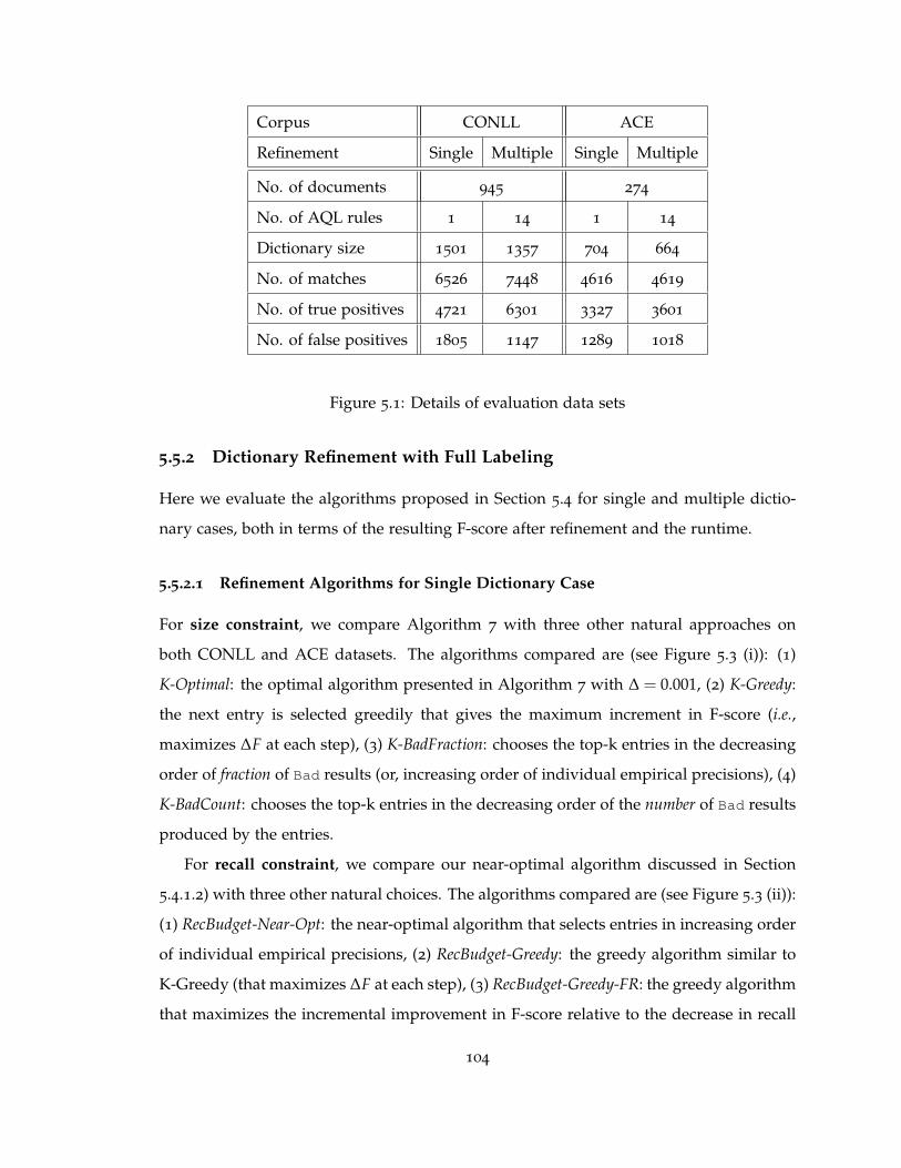
Corpus CONLL ACE

Refinement Single Multiple Single Multiple

No. of documents 945 274

No. of AQL rules 1 14 1 14

Dictionary size 1501 1357 704 664

No. of matches 6526 7448 4616 4619

No. of true positives 4721 6301 3327 3601

No. of false positives 1805 1147 1289 1018

Figure 5.1: Details of evaluation data sets

5.5.2 Dictionary Refinement with Full Labeling

Here we evaluate the algorithms proposed in Section 5.4 for single and multiple dictio-

nary cases, both in terms of the resulting F-score after refinement and the runtime.

5.5.2.1 Refinement Algorithms for Single Dictionary Case

For size constraint, we compare Algorithm 7 with three other natural approaches on

both CONLL and ACE datasets. The algorithms compared are (see Figure 5.3 (i)): (1)

K-Optimal: the optimal algorithm presented in Algorithm 7 with ∆ = 0.001, (2) K-Greedy:

the next entry is selected greedily that gives the maximum increment in F-score (i.e.,

maximizes ∆F at each step), (3) K-BadFraction: chooses the top-k entries in the decreasing

order of fraction of Bad results (or, increasing order of individual empirical precisions), (4)

K-BadCount: chooses the top-k entries in the decreasing order of the number of Bad results

produced by the entries.

For recall constraint, we compare our near-optimal algorithm discussed in Section

5.4.1.2) with three other natural choices. The algorithms compared are (see Figure 5.3 (ii)):

(1) RecBudget-Near-Opt: the near-optimal algorithm that selects entries in increasing order

of individual empirical precisions, (2) RecBudget-Greedy: the greedy algorithm similar to

K-Greedy (that maximizes ∆F at each step), (3) RecBudget-Greedy-FR: the greedy algorithm

that maximizes the incremental improvement in F-score relative to the decrease in recall

104

5e−04 0.003 0.0075 0.03 0.58

Histogram of Bad Fraction of Entries

Fraction of Bad Results

No.

of e

ntrie

s

060

012

00

5e−04 0.003 0.0075 0.03 0.074

Histogram of Frequencies of Entries

(Relative) Frequencies of Entries

No.

of e

ntrie

s

060

012

00

CONLL ACE

[0,1) [1,3) [3,5) [5,10) [10,102)

Histogram of Bad Counts of Entries

Count of Bad Results (CONLL)

No.

of e

ntrie

s

040

080

0

[0,1) [1,3) [3,5) [5,10) [10,454)

Count of Bad Results (ACE)

No.

of e

ntrie

s

020

040

0

Figure 5.2: Histograms for statistics of the data : (i) Fraction of bad results produced by

entries and relative frequencies of entries, (ii) Count of bad results produced by entries.

(i.e., maximizes ∆F/∆R at each step), (4) RecBudget-BadCount: chooses the top-k entries in

the decreasing order of the number of Bad results produced by the entries. Each algorithm

is run until the given recall budget ρ is exhausted.

Observations. For size constraint, K-Optimal and K-Greedy perform better than

selecting by the fraction or number of Bad results, and their performance gap is negligible

on our datasets (Example 5.5 shows that K-Greedy may not give optimal results for some

datasets). On the other hand, for recall constraint, RecBudget-Near-Opt and RecBudget-

Greedy-FR have similar performance and are better than selecting entries by ∆F or the

number of Bad results. In fact, it can be shown that the conditions for these two algorithms

(sorting by fraction of bad results and selecting by ∆F/∆R) are approximately equivalent

assuming both F and R to be continuous functions of entry precisions (i.e., approximating

∆F/∆R by dF/dR).

Figure 5.4 gives the running time of the best two algorithms for both size and recall

constraints, averaged over 100 runs. This figure shows that the algorithms are efficient

and therefore can be embedded in interactive tools. The greedy algorithms take more time

than the (near) optimal algorithms at higher (lower) values of k (ρ). For size constraint,

optimal and greedy respectively run in O(n logn) and O(kn) time, n being the number

105

0 50 100 150 200

0.80

0.85

0.90

0.95

Size Vs F−score

Size (K)

F−s

core

K−Optimal, CONLLK−Greedy, CONLLK−BadFraction, CONLLK−BadCount, CONLL

K−Optimal, ACEK−Greedy, ACEK−BadFraction, ACEK−BadCount, ACE

0.980 0.985 0.990 0.995 1.000

0.86

0.90

0.94

0.98

Recall Vs F−score

Recall

F−s

core

RecBudget−Near−Opt, CONLLRecBudget−Greedy, CONLLRecBudget−Greedy−FR, CONLLRecBudget−BadCount, CONLLRecBudget−Near−Opt, ACERecBudget−Greedy, ACERecBudget−Greedy−FR, ACERecBudget−BadCount, ACE

Figure 5.3: Performance of refinement optimization algorithms for single dictionary: (i)

Size constraint, (ii) Recall constraint

of dictionary entries; the running times are similar for recall constraint. For ∆ = 0.001,

K-Optimal converges in only 5 to 6 iterations. The benefit in running time is expected

more for larger datasets, and therefore K-Optimal and RecBudget-Near-Opt should be

used in practice.

5.5.2.2 Refinement Algorithms for Multiple Dictionary Case

For the multiple dictionary case, we compare the greedy algorithms proposed in Sec-

tion 5.4.2 with other obvious approaches. The algorithms compared for size constraint

are (see Figure 5.5 (i)): (1) K-Greedy: selects the next entry giving maximum ∆F, (2) K-

BadCount: selects the next entry that has produced the maximum number of Bad results,

(3) K-BadFrac: selects the next entry that has the maximum fraction of Bad results among

the results it has produced.

The corresponding algorithms for recall constraint are (1) RecBudget-Greedy-FR (se-

lects the next entry giving maximum ∆F/∆R), (2) RecBudget-BadCount, and (3) RecBudget-

BadFrac (see Figure 5.5 (ii)).

Observations. Figure 5.5 shows that the proposed greedy algorithms perform better

than the other algorithms for both size and recall constraints. Figure 5.4 compares the

106

0 50 100 150 200

01

23

45

67

Size Vs Time

Size (K)

Tim

e (M

illi S

ec)

K−Optimal, CONLLK−Greedy, CONLLK−Optimal, ACEK−Greedy, ACE

0.980 0.985 0.990 0.995 1.000

02

46

8

Recall Budget Vs Time

Recall Budget

Tim

e (M

illi S

ec)

RecBudget−Near−Opt, CONLLRecBudget−Greedy−FR, CONLLRecBudget−Near−Opt, ACERecBudget−Greedy−FR, ACE

Figure 5.4: Running times of refinement algorithms for single dictionary : (i) Size con-

straint, (ii) Recall constraint

running time of the best two algorithms for both size and recall constraints (greedy and

sorting by the fraction of bad results), averaged over 10 runs. Naturally, K-BadFrac and

RecBudget-BadFrac have better running time than the greedy algorithms as they involve

a single round of sorting of the entries. Then the entries are selected according to this

order. The greedy algorithms needs to compute ∆F or ∆F/∆R at each step for every

remaining entry w. This requires deciding whether the provenance expressions of the

results produced by w evaluates to False when w is selected in addition to the entries

already chosen for deletion. The runtime for RecBudget-Greedy-FR is high even at ρ = 1.0

(unlike K-Greedy at k = 0) since even then many entries may get deleted that produce no

Good results. K-Greedy and K-BadFrac give similar F-scores at higher values of k, so

K-BadFrac may be used for some practical purposes at these values of k.

5.5.3 Dictionary Refinement with Incomplete Labeling

Now we evaluate our label estimation approaches for incomplete labeling, i.e., when some

of the results are not labeled as Good or Bad. The label of each unlabeled results will be

estimated using the labeled results using the algorithms in Section 5.3; for the labeled

results, their actual labels will be retained. Our proposed algorithms in Section 5.4 will

107

0 50 100 150 200

0.88

0.90

0.92

0.94

0.96

Size Vs F−score

Size (K)

F−s

core

K−Greedy, CONLLK−BadCount, CONLLK−BadFrac, CONLLK−Greedy, ACEK−BadCount, ACEK−BadFrac, ACE

0.980 0.985 0.990 0.995 1.000

0.90

0.92

0.94

0.96

Recall Vs F−score

Recall

F−s

core

RecBudget−Greedy−FR, CONLLRecBudget−BadCount, CONLLRecBudget−BadFrac, CONLLRecBudget−Greedy−FR, ACERecBudget−BadCount, ACERecBudget−BadFrac, ACE

Figure 5.5: Refinement algorithms for multiple dictionary: (i) Size Vs. F-score, (ii) Recall

budget Vs. F-score

be evaluated on the entire dataset. This we will refer to as the ESTIMATED approach in

the figures (Figure 5.7 and 5.8). The ESTIMATED approach will be compared against the

NOT-ESTIMATED approach, where the algorithms are run only on the labeled result set.

We vary the fraction of labeled results compared to the entire dataset in the figures.

The set of deleted entries returned by each algorithm for both ESTIMATED and NOT-

ESTIMATED approach are evaluated against the actual Good/Bad labels for the entire

resultset to obtain the F-score after refinement. In each run, a random subset of the results

is considered as the labeled resultset according to the desired fraction of labeled results.

The algorithms are repeated for 10 runs, using different random subsets of labeled results

(varying the initial random seed), and the mean F-scores are plotted in Figure 5.7 and 5.8.

5.5.3.1 Incomplete Labeling for Single Dictionary Case

As mentioned in Section 5.3.3 (Observation 5.2), the label of an occurrence produced by

an entry is simply the empirical entry-precision of the entry (fraction of Good counts, and

0.5 if no occurrences are labeled), and therefore, the EM algorithm is not run for this

case. Figure 5.7 (i) shows that, for size constraint, ESTIMATED approach gives better

F-score over NOT-ESTIMATED and the benefit is higher when fewer results are labeled

108

0 50 100 150 200

050

0010

000

1500

0

Size Vs Time

Size (K)

Tim

e (M

illi S

ec)

K−Greedy, CONLLK−BadFrac, CONLLK−Greedy, ACEK−BadFrac, ACE

0.980 0.985 0.990 0.995 1.000

020

0040

0060

0080

00

Recall Budget Vs Time

Recall Budget

Tim

e (M

illi S

ec) RecBudget−Greedy−FR, CONLL

RecBudget−BadFrac, CONLLRecBudget−Greedy−FR, ACERecBudget−BadFrac, ACE

Figure 5.6: Running time for multiple dictionary (i) Size Vs. Time, (ii) Recall Budget Vs.

Time

(both approaches are equivalent when fraction of labeled results = 1). However, for recall

constraint and RecBudget-Near-Opt, both approaches give essentially the same result.

This is as expected, since the entries are chosen according to the fraction of Bad results

which is the same for both labeled and entire resultset.

5.5.3.2 Incomplete Labeling for Multiple Dictionary Case

We first estimate the entry-precisions by the EM algorithm that uses the provenance of

the labeled results (ref. Section 5.3.3) and their labels. The EM algorithm is fast enough

for practical applications (it converges in about 15-20 steps and takes about 2 seconds

to run). Then the label of the unlabeled results are estimated by evaluating their prove-

nance using the estimated entry-precisions (ref. Section 5.3.2). Figure 5.8 shows that

ESTIMATED approach is better or at least as good as the NOT-ESTIMATED approach.

However, the improvement is not as good as the single dictionary case due to the sim-

plified independence assumptions. It will be an important future work to have a more

accurate estimation of the labels incorporating correlations among entries.

109

0.90

00.

910

0.92

0

Effect of Labeled Data Size (Size)

Size of entire data/Size of labeled data

F−s

core

1 2 4 8 16 32

ESTIMATEDNOT−ESTIMATED

0.91

0.93

0.95

0.97

Effect of Labeled Data Size (Recall)

Size of entire data/Size of labeled data

F−s

core

1 2 4 8 16 32

ESTIMATEDNOT−ESTIMATED

Figure 5.7: Effect of the labeled data size on F-score for single dictionary (i) Size constraint,

(ii) Recall constraint.

5.5.3.3 Qualitative Evaluation

We conclude our experiments by qualitatively evaluating the entries returned by our

algorithms on small labeled data. In Figure 5.9, we show some of the entries returned by

our algorithms (the optimal algorithm K-Optimal for size constraint, and the near-optimal

algorithm for recall-constraint RecBudget-Near-Opt) in the single dictionary case. This

figure gives the first 10 entries in an arbitrary run of the algorithms when 1/10-th of the

results are labeled, and shows the counts of Good and Bad results for these entries in both

labeled data and the entire data set. Clearly, these entries are incorrect or ambiguous as

Person names. We see that the entries removed by the near-optimal algorithm for recall

budget are the ones with fraction of Bad results being 1 (they improve precision and F-

score without reducing recall). However, for the optimal under size constraint, entries

with non-zero Good counts may also be chosen as the number of Good and Bad results

also play an important role.

110

0.87

00.

880

0.89

00.

900

Effect of Labeled Data Size (Size)

Size of entire data/Size of labeled data

F−s

core

1 2 4 8 16 32

ESTIMATEDNOT−ESTIMATED

0.87

50.

885

0.89

5

Effect of Labeled Data Size (Recall)

Size of entire data/Size of labeled data

F−s

core

1 2 4 8 16 32

ESTIMATEDNOT−ESTIMATED

Figure 5.8: Effect of the labeled data size on F-score for multiple dictionary (i) Size con-

straint, (ii) Recall constraint.

5.6 Related Work

Previous work on entity extraction from lists on the web (e.g., [73]), open information

extraction (e.g., [8, 177]) and dictionary learning (e.g., [150]) addresses the problem of

creating new dictionaries of terms from unstructured or semi-structured data sources by

exploiting contextual patterns or the structure of web pages. Our work is complemen-

tary to these approaches, and can be used to further refine such automatically generated

dictionaries.

Liu et al. [118] proposed a provenance-based framework for refining information ex-

traction rules. They showed how to use provenance to compute high-level changes, a

specific intermediate result whose removal from the output of an operator causes the

removal of a false positive from the result, and how multiple high-level changes can be

realized via a low-level change: a concrete change to the operator that removes one or

more intermediate results from the output of the operator. While [118] focused on the

general refinement framework based on high-level and low-level changes, it did not go

into depth about the problems of computing specific types of low-level changes. In [151],

we formally study one specific and important type of low-level change, that of refining

111

K-Optimal

(good,bad) Count

Entry Labeled Labeled

+ Unlabeled

china (0, 12) (0, 100)

kong (0, 11) (0, 70)

june (0, 9) (0, 97)

hong (1, 10) (2, 71)

september (0, 8) (0, 101)

king (0, 5) (6, 20)

louis (1, 6) (4, 33)

long (0, 4) (0, 66)

cleveland (0, 4) (0, 30)

april (0, 4) (0, 30)

RecBudget-Near-Opt

(good,bad) Count

Entry Labeled Labeled

+ Unlabeled

china (0, 12) (0, 100)

kong (0, 11) (0, 70)

june (0, 9) (0, 97)

september (0, 8) (0, 101)

king (0, 5) (6, 20)

long (0, 4) (0, 66)

cleveland (0, 4) (0, 30)

april (0, 4) (0, 42)

january (0, 4) (0, 28)

re (0, 4) (0, 54)

Figure 5.9: Top 10 entries output by the (near) optimal algorithms for size and recall

constraints.

dictionaries used in an extractor, especially in the presence of sparse labeled data which

was not considered in [118]. Moreover, our study of the single dictionary refinement

problem is of independent interest: our solution is useful in refining manually or auto-

matically generated dictionaries that can be used as basic features not only in rule-based,

but also statistical (machine learning) information extraction systems.

Also related are recent studies on causality [125] and deletion propagation [35, 108]. In

[125], the input consists of source tuples, an output Boolean vector and a ground truth

Boolean vector, and the goal is to compute the responsibility of every source tuple using

modifications to the source tuples such that the output is identical to the ground truth.

In other words, the modifications should remove all incorrect results, while keeping all

correct results. On the other hand, [35, 108] study the problem of deleting an incorrect

answer tuple of a SPJU query while minimizing the view-side-effect, i.e. the number of

other answer tuples deleted. We consider extractors consisting essentially of SPJU queries,

where dictionary entries correspond to source tuples and extraction results correspond

112

to outputs. As such, our work can be seen as an alternative objective for these related

problems that tries to balance between deletion of incorrect tuples while keeping the

correct tuples. In addition, we seek refinements that generalize well in practice, and do

not restrict ourselves to obtaining the expected extraction result on the labeled data, which

is not useful in our information extraction scenario. To the best of our knowledge, ours is

the first formal study of dictionary refinement for rule-based information extraction.

5.7 Conclusions

In this work, we defined and studied one important aspect of building a high quality in-

formation extraction, that of refining dictionaries used in the extractor. We provided rig-

orous theoretical analysis and experimental evaluation of the optimization problems that

such refinement entails. In addition, we proposed and evaluated statistical approaches

for coping with the scarcity of labeled data. First and foremost, our experimental results

show that dictionary refinement can significantly increase the quality (i.e. F-score) of the

extraction results using even a small amount of labeled data. Further, our experimental

results show which of the several natural baseline refinement algorithms perform bet-

ter on real data sets. Our proposed algorithms and label estimation techniques perform

better than the other approaches.

There are several interesting future directions. So far, we have only considered pos-

itive queries, whereas the difference operation in the extractor rules may be sometimes

necessary. Since dictionaries are expected to contain large number of entries, efficient

handling of large provenance graphs from an extractor with difference operators poses

practical challenges. We would also like to explore a more detailed modeling of correla-

tions between entries and occurrences, as well as analyze the choice of rule refinement.

Finally, since manually labeling results is a time-consuming process, adaptively labeling

a corpus for dictionary refinement given a budget on the number of labels is another

important future direction.

113

Chapter 6

Provenance Views for Module

Privacy

In the previous three chapters, we used Boolean provenance to derive uncertain informa-

tion in the input or the output in the relational setting. In general, data provenance is

useful to understand and debug an experiment or transaction in domains like scientific

research and business processes. These applications involve more complex data (files)

than tuples, and more complicated processes (sophisticated algorithms) than relational

queries. In contrast to fine-grained Boolean provenance, coarse-grained workflow prove-

nance is more useful in this regard, which simply records the data values and processes

used in the generation of a result (see the discussion in Chapter 2). However, substantial

investments in developing a workflow and its components, and the presence of propri-

etary and sensitive elements, restrict publishing and using provenance information in

these domains. In particular, in this dissertation we focus on privacy of proprietary or

commercial modules when they belong to a workflow, which is a key component in sci-

entific research to capture the processes and data flows in an experiment. This chapter

presents our first work in module privacy in workflow provenance, that shows how intention-

ally introducing uncertainty in the provenance information allows publishing provenance

while ensuring module privacy.

114

6.1 Overview

As discussed in Section 2.2, the importance of data provenance has been widely recog-

nized in the context of workflows, a set of modules inter-connected via data paths to

model and formalize a task like scientific experiment or a business process. A module

in a workflow can be abstracted as a function that takes an input and produces an out-

put. Modules used in scientific workflows may be proprietary (e.g., commercial software),

where the owner of the module wants to ensure that the module functionality (i.e., the

output for a given input) is not revealed from the published provenance information. In

[63] we focus on the problem of preserving the privacy of module functionality, i.e. the

mapping between input and output values produced by the module (rather than the

actual algorithm that implements it).

To ensure the privacy of module functionality, we extend the notion of `-diversity [121]

to our network setting36: A module with functionality m in a workflow is said to be Γ-

private if for every input x, the actual value of the output m(x) is indistinguishable from

Γ− 1 other possible values w.r.t. the visible data values in the provenance relation. This

is achieved by carefully selecting a subset of data items and hiding those values in all

executions of the workflow – i.e. by showing the user a view of the provenance relation

for the workflow in which the selected data items (attributes) are hidden. Γ-privacy of a

module ensures that even with arbitrary computational power and access to the view for

all possible executions of workflow, an adversary can not guess the correct value of m(x)

with probability > 1Γ .

To reflect the fact that some data may be more valuable to the user than other data, we

assign a cost to each data item in the workflow, which indicates the utility lost to the user

when the data value is hidden. Identical privacy guarantees can be achieved by hiding

different subsets of data of different cost. Further, a workflow may have data sharing (i.e.

computed data items from a module can be passed as input to more than one module in

the workflow). Therefore hiding some data can be used to guarantee privacy for more

than one module in the network.36In the Related Work, we discuss why a stronger notion of privacy, like differential privacy, is not suitable

here.

115

The problem we address in this work is the following: Given a workflow W, cost of each

data item in the workflow, and a privacy parameter Γ, minimize the cost of hidden data while

guaranteeing that individual private modules in the given workflow are Γ-private. We call this

the secure-view problem. We formally define the problem, study its complexity, and offer

algorithmic solutions. We summarize our contributions in this chapter below.

1. We formalize the notion of Γ-privacy of a private module when it is a standalone

entity (standalone privacy) as well as when it is a component of a workflow (with

arbitrary directed acyclic graph structure and arbitrary data sharing) interacting

with other modules (workflow privacy).

2. For standalone modules, we analyze the computational and communication com-

plexity of obtaining a minimal cost set of input/output data items to hide such that

the remaining, visible attributes guarantee Γ-privacy (a safe subset). We call this the

standalone secure-view problem. Although finding the optimal solution to this prob-

lem has an exponential lower bound on time complexity, we argue that the trivial

exponential-time algorithms to find the optimal solutions or expert-knowledge from

the module designers may be acceptable for a single module having much fewer in-

puts and outputs.

3. Then we study workflows in which all modules are private, i.e. modules for which

the user has no a priori knowledge and whose behavior must be hidden. For such

all-private workflows, we analyze the complexity of finding a minimum cost set of

data items in the workflow, as a whole, to hide such that the remaining visible at-

tributes guarantee Γ-privacy for all modules. We call this the workflow secure-view

problem. Although the privacy of a module within a workflow is inherently linked

to the workflow topology and functionality of other modules, we are able to show

that guaranteeing workflow secure-views in this setting essentially reduces to im-

plementing the standalone privacy requirements for each module. We then study

two variants of the workflow secure-view problem, one in which module privacy

is specified in terms of attribute sets (set constraints) and one in which module pri-

vacy is specified in terms of input/output cardinalities (cardinality constraints). Both

116

variants are easily shown to be NP-hard, and we give poly-time approximation al-

gorithms for these problems. While the cardinality constraints version has an linear-

programming-based O(logn)-approximation algorithm, the set constraints version

is much harder to approximate. However, both variants becomes more tractable

when the workflow has bounded data sharing, i.e. when a data item acts as input to a

small number of modules. In this case a constant factor approximation is possible,

although the problem remains NP-hard even without any data sharing.

4. Then we consider general workflows, i.e workflows which contain private modules as

well as modules whose behavior is known (public modules). Here we show that en-

suring standalone privacy of private modules no longer guarantees their workflow

privacy. However, by making some of the public modules private (privatization) we

can attain workflow privacy of all private modules in the workflow. Since privatiza-

tion has a cost, the optimization problem, becomes much harder: Even without data

sharing the problem is Ω(logn)-hard to approximate. However, for both all-private

and general workflows, there is an LP-based `max-approximation algorithm, where

`max is the length of longest requirement list for any module.

Organization. Section 6.2 formalizes the notions of Γ-privacy of a module, both when

it is standalone and when it appears in a workflow. The secure-view problem for stan-

dalone module privacy is studied in Section 6.3. Section 6.4 then studies the problem for

workflows consisting only of private modules, whereas Section 6.5 generalizes the results

to general workflows consisting of both public and private modules. Finally we conclude

and discuss directions for future work in Section 6.7.

6.2 Module Privacy

Here we formally define module privacy with respect to workflow provenance. We first

consider the privacy of a single module, which we call standalone module privacy. Then

we consider privacy when modules are connected in a workflow, which we call workflow

module privacy.

117

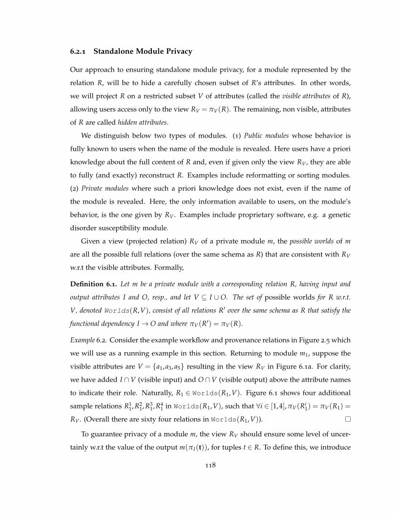
6.2.1 Standalone Module Privacy

Our approach to ensuring standalone module privacy, for a module represented by the

relation R, will be to hide a carefully chosen subset of R’s attributes. In other words,

we will project R on a restricted subset V of attributes (called the visible attributes of R),

allowing users access only to the view RV = πV(R). The remaining, non visible, attributes

of R are called hidden attributes.

We distinguish below two types of modules. (1) Public modules whose behavior is

fully known to users when the name of the module is revealed. Here users have a priori

knowledge about the full content of R and, even if given only the view RV , they are able

to fully (and exactly) reconstruct R. Examples include reformatting or sorting modules.

(2) Private modules where such a priori knowledge does not exist, even if the name of

the module is revealed. Here, the only information available to users, on the module’s

behavior, is the one given by RV . Examples include proprietary software, e.g. a genetic

disorder susceptibility module.

Given a view (projected relation) RV of a private module m, the possible worlds of m

are all the possible full relations (over the same schema as R) that are consistent with RV

w.r.t the visible attributes. Formally,

Definition 6.1. Let m be a private module with a corresponding relation R, having input and

output attributes I and O, resp., and let V ⊆ I ∪O. The set of possible worlds for R w.r.t.

V, denoted Worlds(R,V), consist of all relations R′ over the same schema as R that satisfy the

functional dependency I→O and where πV(R′) = πV(R).

Example 6.2. Consider the example workflow and provenance relations in Figure 2.5 which

we will use as a running example in this section. Returning to module m1, suppose the

visible attributes are V = a1, a3, a5 resulting in the view RV in Figure 6.1a. For clarity,

we have added I ∩V (visible input) and O ∩V (visible output) above the attribute names

to indicate their role. Naturally, R1 ∈ Worlds(R1,V). Figure 6.1 shows four additional

sample relations R11, R2

1, R31, R4

1 in Worlds(R1,V), such that ∀i ∈ [1,4],πV(Ri1) = πV(R1) =

RV . (Overall there are sixty four relations in Worlds(R1,V)).

To guarantee privacy of a module m, the view RV should ensure some level of uncer-

tainly w.r.t the value of the output m(πI(t)), for tuples t ∈ R. To define this, we introduce

118

I ∩V O ∩V

a1 a3 a5

0 0 1

0 1 0

1 1 0

1 1 1

(a) RV = πV(R1) for

V=a1, a3, a5

a1 a2 a3 a4 a5

0 0 0 0 1

0 1 1 0 0

1 0 1 0 0

1 1 1 0 1

(b) R11

a1 a2 a3 a4 a5

0 0 0 1 1

0 1 1 1 0

1 0 1 0 0

1 1 1 0 1

(c) R21

a1 a2 a3 a4 a5

0 0 1 0 0

0 1 0 0 1

1 0 1 0 0

1 1 1 0 1

(d) R31

a1 a2 a3 a4 a5

0 0 1 1 0

0 1 0 1 1

1 0 1 0 0

1 1 1 0 1

(e) R41

Figure 6.1: (a): Projected relation for m1 when attribute a2, a4 are hidden, (b)-(d): Ri1 ∈

Worlds(R1,V), i ∈ [1,4]

the notion of Γ-standalone-privacy, for a given parameter Γ ≥ 1. Informally, RV is Γ-

standalone-private if for every t ∈ R, the possible worlds Worlds(R,V) contain at least Γ

distinct output values that could be the result of m(πI(t)). Note that, a view RV “hides”

some data values in the provenance relations by access control, and the user cannot see or

access the hidden values.

Definition 6.3. Let m be a private module with a corresponding relation R having input and

output attributes I and O resp. Then m is Γ-standalone-private w.r.t a set of visible attributes V,

if for every tuple x ∈ πI(R), |OUTx,m| ≥ Γ, where OUTx,m = y | ∃R′ ∈ Worlds(R,V), ∃t′ ∈

R′ s.t x = πI(t′) ∧ y = πO(t′).

If m is Γ-standalone-private w.r.t. V, then we will call V a safe subset for m and Γ.

Γ-standalone-privacy implies that for any input the adversary cannot guess m’s output

with probability > 1Γ , even if the module is executed an arbitrary number of times.

119

Example 6.4. It can be verified that, if V = a1, a3, a5 then for all x ∈ πI(R1), |OUTx| ≥

4, so a1, a3, a5 is safe for m1 and Γ = 4. As an example, from Figure 6.1, when x =

(0,0), OUTx,m ⊇ (0,0,1), (0,1,1), (1,0,0), (1,1,0) (hidden attributes are underlined). Also,

hiding any two output attributes from O = a3, a4, a5 ensures standalone privacy for

Γ = 4, e.g., if V = a1, a2, a3 (i.e. a4, a5 are hidden), then the input (0,0) can be mapped

to one of (0,0,0), (0,0,1), (0,1,0) and (0,1,1); this holds for other assignments of input

attributes as well. But, V = a3, a4, a5 (i.e. when only input attributes are hidden) is not

safe for Γ = 4: for any input x, OUTx,m = (0,1,1), (1,1,0), (1,0,1), containing only three

possible output tuples.

There may be several safe subsets V for a given module m and parameter Γ. Some

of the corresponding RV views may be preferable to others, e.g. they provide users with

more useful information, allow to answer more common/critical user queries, etc. Let

V = (I ∪ O) \ V denote the attributes of R that do not belong to the view. If c(V)

denotes the penalty of hiding the attributes in V, a natural goal is to choose a safe subset

V that minimizes c(V). To understand the difficulty of this problem, we study a version

of the problem where the cost function is additive: each attribute a has some penalty

value c(a) and the penalty of hiding V is c(V) = Σa∈V c(a). We call this optimization

problem the standalone Secure-View problem and discuss it in Chapter 6.

6.2.1.1 Workflow Module Privacy

To define privacy in the context of a workflow, we first extend our notion of possible worlds

to a workflow view. Consider the view RV = πV(R) of a workflow relation R. Since the

workflow may contain private as well as public modules, a possible world for RV is a full

relation that not only agrees with RV on the content of the visible attributes, but is also

consistent w.r.t the expected behavior of the public modules. In the following definitions,

m1, · · · ,mn denote the modules in the workflow W and F denotes the set of functional

dependencies Ii→Oi, i ∈ [1,n] in the relation R.

Definition 6.5. The set of possible worlds for the workflow relation R w.r.t. V, denoted also

Worlds(R,V), consists of all the relations R′ over the same attributes as R that satisfy the

functional dependencies in F and where (1) πV(R′) = πV(R), and (2) for every public module mi

120

in W and every tuple t′ ∈ R′, πOi(t′) = mi(πIi(t

′)).

Note that when a workflow consists only of private modules, the second constraint

does not need to be enforced. We call these all-private workflows and study them in Chap-

ter 6. We discuss workflows with both public and private modules in Chapter 6 and

7, and argue that attaining privacy in the presence of public modules is fundamentally

harder.

We are now ready to define the notion of Γ-workflow-privacy, for a given parameter

Γ ≥ 1. Informally, a view RV is Γ-workflow-private if for every tuple t ∈ R, and every

private module mi in the workflow, the possible worlds Worlds(R,V) contain at least Γ

distinct output values that could be the result of mi(πIi(t)).

Definition 6.6. A private module mi in W is Γ-workflow-private w.r.t a set of visible attributes

V, if for every tuple x ∈ πIi(R), |OUTx,W | ≥ Γ, where OUTx,W = y | ∃R′ ∈ Worlds(R,V),

s.t., ∀t′ ∈ R′ x = πIi(t′)⇒ y = πOi(t

′).

W is called Γ-private if every private module mi in W is Γ-workflow-private. If W (resp.

mi) is Γ-private (Γ-workflow-private) w.r.t. V, then we call V a safe subset for Γ-privacy of W

(Γ-workflow-privacy of mi).

For simplicity, in the above definition we assumed that the privacy requirement of ev-

ery module mi is the same Γ. The results and proofs in Chapter 6 and 7 remain unchanged

when different modules mi have different privacy requirements Γi.

In these chapters, for a set of visible attributes V ⊆ A, V = A \ V will denote the

hidden attributes in the workflow. The following proposition is easy to verify, and will be

used in our proofs:

Proposition 6.7. If V is a safe subset for Γ-workflow-privacy of a module mi in W, then any V ′

such that V ′ ⊆ V (or, V ′ ⊇ V) also guarantees Γ-workflow-privacy of mi.

As we illustrate later, given a workflow W and a parameter Γ there may be several

incomparable (in terms of set inclusion) safe subsets V for Γ-privacy of W. Our goal is

to choose one that minimizes the penalty c(V) = Σa∈V c(a) of the hidden attributes V.

This we call the workflow Secure-View problem, or simply the Secure-View problem,

and study this optimization problem in Chapter 6 and 7.

121

In our complexity results, we will see the implication of limited data sharing, i.e., when

the output of a module is fed as input to several modules in a workflow. We define the

degree of data sharing in a workflow as follows:

Definition 6.8. A workflow W is said to have γ-bounded data sharing if every attribute in W

can appear in the left hand side of at most γ functional dependencies Ii→Oi.

In the workflow in Figure 2.5, γ = 2. Intuitively, if a workflow has γ-bounded data

sharing then a data item can be fed as input to at most γ different modules.

6.3 Standalone Module Privacy

We start our study of workflow privacy by considering the privacy of a standalone mod-

ule, which is the simplest special case of a workflow. Hence understanding it is a first

step towards understanding the general case. We will also see that standalone-privacy

guarantees of individual modules may be used as building blocks for attaining workflow

privacy.

We analyze below the time complexity of obtaining (minimal cost) guarantees for

standalone module privacy. Though the notion of Γ-standalone-privacy is similar to the

well-known notion of `-diversity [121], to the best of our knowledge the time complexity

of this problem has not been studied.

Optimization problems and parameters. Consider a standalone module m with input

attributes I, output attributes O, and a relation R. Recall that a visible subset of attributes

V is called a safe subset for module m and privacy requirement Γ, if m is Γ-standalone-

private w.r.t. V (see Definition 6.3). If each attribute a ∈ I ∪O has cost c(a), the standalone

Secure-View problem aims to find a safe subset V s.t. the cost of the hidden attributes,

c(V) = ∑a∈V c(a), is minimized. The corresponding decision version will take a cost

limit C as an additional input, and decide whether there exists a safe subset V such that

c(V) ≤ C.

One natural way of solving the optimization version of the standalone Secure-View

problem is to consider all possible subsets V ⊆ I ∪O, check if V is safe, and return the

122

safe subset V s.t. c(V) is minimized. This motivates us to define and study the simpler

Safe-View problem, which takes a subset V as input and decides whether V is a safe

subset.

To understand how much of the complexity of the standalone Secure-View problem

comes from the need to consider different subsets of attributes, and what is due to the

need to determine the safety of subsets, we study the time complexity of standalone

Secure-View, with and without access to an oracle for the Safe-Viewproblem, henceforth

called a Safe-View oracle. A Safe-Vieworacle takes a subset V ⊆ I ∪O as input and

answers whether V is safe. In the presence of a Safe-View oracle, the time complexity

of the Safe-View problem is mainly due to the number of oracle calls, and hence we

study the communication complexity. Without access to such an oracle, we also study the

computational complexity of this problem.

In our discussion below, k = |I| + |O| denotes the total number of attributes in the

relation R, and N denotes the number of rows in R (i.e. the number of executions). Then

N ≤ ∏a∈I |∆a| ≤ δ|I| ≤ δk where ∆a is the domain of attribute a and δ is the maximum

domain size of attributes.

6.3.1 Lower Bounds

We start with lower bounds for the Safe-View problem. Observe that this also gives

lower bounds for the standalone Secure-View problem without a Safe-View oracle.

To see this, consider a set V of attributes and assume that each attribute in V has cost > 0

whereas all other attributes have cost zero. Then Safe-View has a positive answer for V

iff the standalone Secure-View problem has a solution with cost = 0 (i.e. one that hides

only the attributes V).

Communication complexity of Safe-View. Given a visible subset V ⊆ I ∪O, we show

that deciding whether V is safe needs Ω(N) time. Note that just to read the table as input

takes Ω(N) time. So the lower bound of Ω(N) does not make sense unless we assume

the presence of a data supplier (we avoid using the term “oracle” to distinguish it from

Safe-View oracle) which supplies the tuples of R on demand: Given an assignment

x of the input attributes I, the data supplier outputs the value y = m(x) of the output

123

attributes O. The following theorem shows the Ω(N) communication complexity lower

bound in terms of the number of calls to the data supplier; namely, that (up to a constant

factor) one indeed needs to view the full relation.

Theorem 6.9. (Safe-View Communication Complexity) Given a module m, a subset V ⊆

I ∪O, and a privacy requirement Γ, deciding whether V is safe for m and Γ requires Ω(N) calls

to the data supplier, where N is the number of tuples in the relation R of m.

Proof sketch. This theorem is proved by a reduction from the set-disjointness problem, where

Alice and Bob hold two subsets A and B of a universe U and the goal is decide whether

A ∩ B 6= φ. This problem is known to have Ω(N) communication complexity where N is

the number of elements in the universe (details are in Appendix A.4.1).

Computational Complexity of Safe-View: The above Ω(N) computation complexity

of Safe-View holds when the relation R is given explicitly tuple by tuple. The following

theorem shows that even when R is described implicitly in a succinct manner, there cannot

be a poly-time (in the number of attributes) algorithm to decide whether a given subset

V is safe unless P = NP (proof is in Appendix A.4.2).

Theorem 6.10. (Safe-View Computational Complexity) Given a module m with a poly-

size (in k= |I|+ |O|) description of functionality, a subset V ⊆ I ∪O, and a privacy requirement

Γ, deciding whether V is safe w.r.t. m and Γ is co-NP-hard in k.

Proof sketch. The proof of this theorem works by a reduction from the UNSAT prob-

lem, where given a Boolean CNF formula g on variables x1, · · · , x`, the goal is to decide

whether, for all assignments of the variables, g is not satisfiable. Here given any assign-

ment of the variables x1, · · · , x`, g(x1, · · · , x`) can be evaluated in polynomial time, which

simulates the function of the data supplier.

Lower Bound of Standalone Secure-View with a Safe-View Oracle: Now sup-

pose we have access to a Safe-View oracle, which takes care of the “hardness” of the

Safe-View problem given in Theorems 6.9 and 6.10, in constant time. The oracle takes

a visible subset V ⊆ I ∪O as input, and answers whether V is safe for module m and pri-

vacy requirement Γ. The following theorem shows that the decision version of standalone

Secure-View remains hard (i.e. not solvable in poly-time in the number of attributes):

124

Theorem 6.11. (Standalone Secure-View Communication Complexity, with

Safe-View oracle) Given a Safe-View oracle and a cost limit C, deciding whether there exists

a safe subset V ⊆ I ∪O with cost bounded by C requires 2Ω(k) oracle calls, where k = |I|+ |O|.

Proof sketch. The proof of this theorem involves a novel construction of two functions, m1

and m2, on ` input attributes and a single output attribute, such that for m1 the minimum

cost of a safe subset is 3`4 whereas for m2 it is `

2 (C = `2 ). In particular, for both m1 and m2,

all subsets of size < `4 are safe and all other subsets are unsafe, except that for m2, there is

exactly one special subset of size `2 such that this subset and all subsets thereof are safe.

We show that for an algorithm using 2o(k) calls, there always remains at least one

special subset of size `2 that is consistent with all previous answers to queries. Hence

after 2o(k) calls, if the algorithm decides that there is a safe subset with cost ≤ C, we

choose m to be m1; on the other hand, if it says that there is no such subset, we set

m = m2. In both the cases the answer of the algorithm is wrong which shows that there

cannot be such an algorithm distinguishing these two cases with 2o(k) calls (details appear

in Appendix A.4.3).

6.3.2 Upper Bounds

The lower bound results given above show that solving the standalone Secure-View

problem is unlikely in time sub-exponential in k or sub-linear in N. We now present

algorithms for solving the Secure-View and Safe-View problems, in time polynomial

in N and exponential in k.

First note that, with access to a Safe-View oracle, the standalone Secure-View

problem can be easily solved in O(2k) time, by calling the oracle for all 2k possible subsets

and outputting the safe subset with minimum cost.

Without access to a Safe-View oracle, we first “read” relation R using N data sup-

plier calls. Once R is available, the simple algorithm sketched below implements the

Safe-View oracle (i.e. tests if a set V of attributes is safe) and works in time O(2kN2):

For a visible subset V, we look at all possible assignments to the attributes in I \ V. For

each input value we then check if it leads to at least Γ∏a∈O\V |∆a| different values of the

visible output attributes in O ∩ V (∆a is the domain of attribute a). This is a necessary

125

and sufficient condition for guaranteeing Γ privacy, since by all possible ∏a∈O\V |∆a| ex-

tensions of the output attributes, for each input, there will be Γ different possible output

values. The algorithm is simple and details can be found in [64]. We mention here also

that essentially the same algorithms (with same upper bounds) can be used to output all

safe attribute sets of a standalone module, rather than just one with minimum cost. Such

exhaustive enumeration will be useful in the following sections.

Remarks. These results indicate that, in the worse case, finding a minimal-cost safe at-

tribute set for a module may take time that is exponential in the number of attributes.

Note, however, that the number of attributes of a single module is typically not large (of-

ten less than 10, see [2]), so the computation is still feasible. Expert knowledge of module

designers, about the module’s behavior and safe attribute sets may also be exploited to

speed up the computation. Furthermore, a given module is often used in many work-

flows. For example, sequence comparison modules, like BLAST or FASTA, are used in

many different biological workflows. We will see that safe subsets for individual mod-

ules can be used as building blocks for attaining privacy for the full workflow. The effort

invested in deriving safe subsets for a module is thus amortized over all uses.

6.4 All-Private Workflows

We are now ready to consider workflows that consist of several modules. We first con-

sider in this section workflows where all modules are private (called all-private workflows).

Workflows with a mixture of private and public modules are then considered in Section

6.5.

As in Section 6.3, we want to find a safe visible subset V with minimum cost s.t. all the

modules in the workflow are Γ-workflow-private w.r.t. V (see Definition 6.6). One option

is to devise algorithms similar to those described for standalone modules in the previous

section. However, the time complexity of those algorithms is now exponential in the total

number of attributes of all modules in the workflow which can be as large as Ω(nk), n being

the number of modules in the workflow and k the maximum number of attributes of a

single module. To avoid the exponential dependency on n, the number of modules in the

126

workflow,which may be large [2], and to exploit the safe attribute subsets for standalone

modules, which may have been already computed, we attempt in this section to assemble

workflow privacy guarantees out of standalone module guarantees. We first prove, in

Section 6.4.1, that this is indeed possible. Then, in the rest of this section, we study the

optimization problem of obtaining a safe view with minimum cost.

Let W be a workflow consisting of modules m1, · · · ,mn, where Ii,Oi denote the input

and output attributes of mi, i ∈ [1,n], respectively. We use below Ri to denote the relation

for the standalone module mi. The relations R = R1 1 R2 1 · · · 1 Rn, with attributes A =⋃n1=1(Ii ∪Oi), then describes the possible executions of W. Note that if one of the modules

in W is not a one-to-one function then the projection πIi∪Oi(R) of the relation R on Ii ∪Oi

may be a subset of the (standalone) module relation Ri.

In this section (and throughout the rest of the chapter), for a set of visible attributes

V ⊆ A, V = A \ V will denote the hidden attributes. Further, Vi = (Ii ∪ Oi) ∩ V will

denote the visible attributes for module mi, whereas Vi = (Ii ∪Oi) \ Vi will denote the

hidden attributes for mi, for i ∈ [1,n].

6.4.1 Standalone-Privacy vs. Workflow-Privacy

We show that if a set of visible attributes guarantees Γ-standalone-privacy for a module,

then if the module is placed in a workflow where only a subset of those attributes is

made visible, then Γ-workflow-privacy is guaranteed for the module in this workflow. In

other words, in an all-private workflow, hiding the union of the corresponding hidden

attributes of the individual modules guarantees Γ-workflow-privacy for all of them37. We

formalize this next.

Theorem 6.12. Let W be an all-private workflow with modules m1, · · · ,mn. Given a parameter

Γ ≥ 1, let Vi ⊆ (Ii ∪Oi) be a set of visible attributes w.r.t which mi, i ∈ [1,n], is Γ-standalone-

private. Then the workflow W is Γ-private w.r.t the set of visible attributes V s.t. V =⋃n

i=1 Vi.

Before we prove the theorem, recall that Γ-standalone-privacy of a module mi requires

that for every input x to the module, there are at least Γ potential outputs of x in the

37By Proposition 6.7, this also means that hiding any superset of this union would also be safe for the same

privacy guarantee.

127

possible worlds Worlds(Ri,Vi) of the standalone module relation Ri w.r.t. Vi; similarly,

Γ-workflow-privacy of mi requires at least Γ potential outputs of x in the possible worlds

Worlds(R,V) of the workflow relation R w.r.t. V. Since R = R1 1 · · · 1 Rn, a possible ap-

proach to prove Theorem 6.12 may be to show that, whenever the hidden attributes for mi

are also hidden in the workflow W, any relation R′i ∈ Worlds(Ri,Vi) has a corresponding

relation R′ ∈ Worlds(R,V) s.t. R′i = πIi∪Oi(R′). If this would hold, then for V =⋃n

i=1 Vi,

the set of possible outputs, for any input tuple x to a module mi, will remain unchanged.

Unfortunately, Proposition 6.13 below shows that the above approach fails. Indeed,

|Worlds(R,V)| can be significantly smaller than |Worlds(Ri,Vi)| even for very simple

workflows.

Proposition 6.13. There exist a workflow W with relation R, a module m1 in W with (standalone)

relation R1, and a set of visible attributes V1 that guarantees both Γ-standalone-privacy and Γ-

workflow-privacy of m1, such that the ratio of |Worlds(R1,V1)| and |Worlds(R,V1)| is doubly

exponential in the number of attributes of W.

Proof sketch. To prove the proposition, we construct a simple workflow with two modules

m1,m2 connected as a chain. Both m1,m2 are one-one functions with k Boolean inputs

and k Boolean outputs (for example, assume that m1 is an identity function, whereas

m2 reverses the values of its k inputs). The module m1 gets initial input attribute set I1,

produces O1 = I2 which is fed to the module m2 as input, and m2 produces final attribute

set O2. Let V1 be an arbitrary subset of O1 such that |V1| = logΓ (we assume that Γ is a

power of 2). It can be verified that, m1 as a standalone module is Γ-standalone-private

w.r.t. visible attributes V1 and both m1,m2, being one-one modules, are Γ-workflow-

private w.r.t. V1.

We show that the one-one nature of m1 and m2 restricts the size of Worlds(R,V1)

compared to that of Worlds(R1,V1). Since both m1 and m2 are one-one functions, the

workflow W also computes a one-one function. Hence any relation S in Worlds(R,V1)

has to compute a one-one function as well. But when m1 was standalone, any function

consistent with V1 could be a member of Worlds(R1,V1). By a careful computation, the

ratio can be shown to be doubly exponential in k (details appear in Appendix A.4.4).

Nevertheless, we show below that for every input x of the module, the set of its

128

possible outputs, in these worlds, is exactly the same as that in the original (much larger

number of) module worlds. Hence privacy is indeed preserved.

In proving Theorem 6.12, our main technical tool is Lemma 6.14, which states that

given a set of visible attributes Vi of a standalone module mi, the set of possible outputs

for every input x to mi remains unchanged when mi is placed in an all-private workflow,

provided the corresponding hidden attributes Vi remains hidden in the workflow.

Recall that OUTx,mi and OUTx,W denote the possible output for an input x to module mi

w.r.t. a set of visible attributes when mi is standalone and in a workflow W respectively

(see Definition 6.3 and Definition 6.6).

Lemma 6.14. Consider any module mi and any input x ∈ πIi(R). If y ∈ OUTx,mi w.r.t. a set of

visible attributes Vi ⊆ (Ii ∪Oi), then y ∈ OUTx,W w.r.t. Vi ∪ (A \ (Ii ∪Oi)).

The above lemma directly implies Theorem 6.12:

of Theorem 6.12. We are given that each module mi is Γ-standalone-private w.r.t. Vi, i.e.,

|OUTx,mi | ≥ Γ for all input x to mi, for all modules mi, i ∈ [1,n] (see Definition 6.3). From

Lemma 6.14, this implies that for all input x to all modules mi, |OUTx,W | ≥ Γ w.r.t V ′ =

Vi ∪ (A \ (Ii ∪ Oi)). For this choice of V ′, V ′ = A \ V ′ = (Ii ∪ Oi) \ Vi = Vi (because,

Vi ⊆ Ii ∪Oi ⊆ A). Now, using Proposition 6.7, when the visible attributes set V is such

that V =⋃n

i=1 Vi ⊇ Vi = V ′, every module mi is Γ-workflow-private.

To conclude the proof of Theorem 6.12 we thus only need to prove Lemma 6.14. For

this, we use the following auxiliary lemma.

Lemma 6.15. Let mi be a standalone module with relation Ri, let x be an input to mi, and let

Vi⊆ (Ii ∪Oi) be a subset of visible attributes. If y∈OUTx,mi then there exists an input x′ ∈πIi(Ri)

to mi with output y′ = mi(x′) such that πVi∩Ii(x) = πVi∩Ii(x′) and πVi∩Oi(y) = πVi∩Oi(y

′).

The statement of the lemma can be illustrated with the module m1 whose relation

R1 appears Figure 2.5b. Its visible portion (for visible attributes a1, a3, a5) is given in

Figure 6.1a. Consider the input x = (0,0) to m1 and the output y = (1,0,0). For V =

a1, a3, a5, y ∈ OUTx,m1 (see Figure 6.1d). This is because there exists x′ = (0,1), s.t. y′ =

m1(x′) = (1,1,0), and, x,x′ and y,y′ have the same values of the visible attributes (a1 and

129

a3, a5 respectively). Note that y does not need to be the actual output m1(x) on x or

even share the same values of the visible attributes (indeed, m1(x) = (0,1,1)). We defer

the proof of Lemma 6.15 to Appendix A.4.5 and instead briefly explain how it is used to

prove Lemma 6.14.

Proof sketch of Lemma 6.14. Let us fix a module mi, an input x to mi and a candidate output

y ∈ OUTx,mi for x w.r.t. visible attributes Vi. We already argued that, for V = Vi ∪ (A \

(Ii ∪Oi)), V = A \ V = (Ii ∪Oi) \ Vi = Vi. We will show that y ∈ OUTx,W w.r.t. visible

attributes V by showing the existence of a possible world R′ ∈ Worlds(R,V), for V = Vi,

s.t. πIi(t) = x and πOi(t) = y for some t ∈ R′.

We start by replacing module mi by a new module gi such that gi(x) = y as required.

But due to data sharing, other modules in the workflow can have input and output at-

tributes from Ii and Oi. Hence if we leave the modules mj, j 6= i, unchanged, there may be

inconsistency in the values of the visible attributes, and the relation produced by the join

of the standalone relations of the module sequence 〈m1, · · · ,mi−1, gi,mi+1, · · · ,mn〉may not

be a member of Worlds(R,V). To resolve this, we consider the modules in a topological

order, and change the definition of all modules m1, · · · ,mn to g1, · · · , gn (some modules

may remain unchanged). In proving the above, the main idea is to use tuple and function

flipping (formal definition in the appendix). If a module mj shares attributes from Ii or

Oi, the new definition gj of mj involves flipping the input to mj, apply mj on this flipped

input, and then flipping the output again to the output value. The proof shows that by

consistently flipping all modules, the visible attribute values remain consistent with the

original workflow relation and we get a member of the possible worlds (details appear in

Appendix A.4.6).

It is important to note that the assumption of all-private workflow is crucial in proving

Lemma 6.14 – if some of the modules mj are public, we can not redefine them to gj (the

projection to the public modules should be unchanged - see Definition 6.6) and we may

not get a member of Worlds(R,V). We will return to this point in Section 6.5 when we

consider workflows with a mixture of private and public modules.

130

6.4.2 The Secure-View Problem

We have seen above that one can assemble workflow privacy guarantees out of the stan-

dalone module guarantees. Recall however that each individual module may have several

possible safe attributes sets (see, e.g., Example 6.4). Assembling different sets naturally

lead to solutions with different cost. The following example shows that assembling

optimal (cheapest) safe attributes of the individual modules may not lead to an optimal

safe attributes set for the full workflow. The key observation is that, due to data sharing,

it may be more cost effective to hide expensive shared attributes rather than cheap non-

shared ones (though later we show that the problem remains NP-hard even without data

sharing).

Example 6.16. Consider a workflow with n + 2 modules, m,m1, · · · ,mn,m′. The module

m gets an input data item a1, with cost 1, and sends as output the same data item, a2,

with cost 1 + ε, ε > 0, to all the mi-s. Each mi then sends a data item bi to m′ with cost

1. Assume that standalone privacy is preserved for module m if either its incoming or

outgoing data is hidden and for m′ if any of its incoming data is hidden. Also assume that

standalone privacy is preserved for each mi module if either its incoming or its outgoing

data is hidden. As standalone modules, m will choose to hide a1, each mi will choose

to hide the outgoing data item bi, and m′ will choose to hide any of the bi-s. The union

of the optimal solutions for the standalone modules has cost n + 1. However, a lowest

cost solution for preserving workflow privacy is to hide a2 and any one of the bi-s. This

assembly of (non optimal) solutions for the individual modules has cost 2 + ε. In this

case, the ratio of the costs of the union of standalone optimal solutions and the workflow

optimal solution is Ω(n).

This motivates us to define the combinatorial optimization problem Secure-View

(for workflow secure view), which generalizes the Secure-View problem studied in

Section 6.3. The goal of the Secure-View problem is to choose, for each module, a safe

set of attributes (among its possible sets of safe attributes) s.t. together the selected sets

yield a minimal cost safe solution for the workflow. We define this formally below. In par-

ticular, we consider the following two variants of the problem, trading-off expressibility

and succinctness.

131

Set constraints. The possible safe solutions for a given module can be given in the

form of a list of hidden attribute sets. Specifically, we assume that we are given, for each

module mi, i ∈ [1,n], a list of pairs Li = 〈(I1i ,O1

i ), (I2i ,O2

i ) . . . (I lii ,Oli

i )〉. Each pair (I ji ,O

ji) in

the list describes one possible safe (hidden) solution for mi: I ji ⊆ Ii (resp. Oj

i ⊆ Oi) is the

set of input (output) attributes of mi to be hidden in this solution. li (the length of the

list) is the number of solutions for mi that are given in the list, and we use below `max to

denote the length of the longest list, i.e. `max = maxni=1 `i.

When the input to the Secure-View problem is given in the above form (the can-

didate attribute sets are listed explicitly), we call it the Secure-View problem with set

constraints.

Cardinality constraints. Some modules may have many possible candidate safe attribute

sets. Indeed, their number may be exponential in the number of attributes of the module.

This is illustrate by the following two simple examples.

Example 6.17. First observe that in any one-one function with k Boolean inputs and k

Boolean outputs, hiding any k incoming or any k outgoing attributes guarantees 2k-

privacy. Thus listing all such subsets requires a list of length Ω((2kk )) = Ω(2k). Another

example is majority function which takes 2k Boolean inputs and produces 1 if and only if

the number of one-s in the input tuple is ≥ k. Hiding either k + 1 input bits or the unique

output bit guarantee 2-privacy for majority function, but explicitly listing all possible

subsets again leads to exponential length lists.

Note that, in both examples, the actual identity of the hidden input (resp. output)

attributes is not important, as long as sufficiently many are hidden. Thus rather than

explicitly listing all possible safe sets we could simply say what combinations of numbers

of hidden input and output attributes are safe. This motivates the following variant of

the Secure-View problem, called the Secure-View problem with cardinality constraints:

Here for every module mi we are given a list of pairs of numbers Li = 〈(α1i , β1

i ) . . . (αlii , βli

i )〉,

s.t. for each pair (αji , β

ji) in the list, α

ji ≤ |Ii| and β

ji ≤ |Oi|. The interpretation is that hiding

any attribute set of mi that consists of at least αji input attributes and at least β

ji output

attributes, for some j ∈ [1,`i], makes mi safe w.r.t the remaining visible attributes.

To continue with the above example, the list for the first module may consists of (k,0)

132

and (0,k), whereas the list for the second module consists of (k + 1,0) and (0,1).

It is easy to see that, for cardinality constraints, the lists are of size at most quadratic

in the number of attributes of the given module (unlike the case of set constraints where

the lists could be of exponential length)38. In turn, cardinality constraints are less ex-

pressive than set constraints that can specify arbitrary attribute sets. This will affect the

complexity of the corresponding Secure-View problems.

Problem Statement. Given an input in one of the two forms, a feasible safe subset V for

the workflow, for the version with set constraints (resp. cardinality constraints), is such

that for each module mi i ∈ [1,n], V ⊇ (I ji ∪Oj

i) (resp. |V ∩ Ii| ≥ αji and |V ∩Oi| ≥ β

ji)

for some j ∈ [1,`i]. The goal of the Secure-View problem is to find a safe set V where

c(V) is minimized.

6.4.3 Complexity results

We present below theorems which give approximation algorithms and matching hard-

ness of approximation results of different versions of the Secure-View problem. The

hardness results show that the problem of testing whether the Secure-View problem

(in both variants) has a solution with cost smaller than a given bound is NP-hard even in

the most restricted case. But we show that certain approximations of the optimal solution

are possible. Theorem 6.18 and 6.20 summarize the results for the cardinality and set

constraints versions, respectively. Here we only sketch the proofs for brevity; full details

appear in Appendix A.4.7.

Theorem 6.18. (Cardinality Constraints) There is an O(logn)-approximation of the

Secure-View problem with cardinality constraints. Further, this problem is Ω(logn)-hard to

approximate unless NP ⊆ DTIME(nO(loglogn)), even if the maximum list size `max = 1, each

data has unit cost, and the values of αji , β

ji-s are 0 or 1.

Proof sketch. The proof of the hardness result in the above theorem is by a reduction

from the set cover problem. The approximation is obtained by randomized rounding a

carefully written linear program (LP) relaxation of this problem. A sketch is given below.

38In fact, if one assumes that there is no redundancy in the list, the lists become of at most of linear size.

133

Our algorithm is based on rounding the fractional relaxation (called the LP relaxation)

of the integer linear program (IP) for this problem presented in Figure 6.2.

Minimize ∑b∈A cbxb subject to

`i

∑j=1

rij ≥ 1 ∀i ∈ [1,n] (6.1)

∑b∈Ii

ybij ≥ rijαji ∀i ∈ [1,n], ∀j ∈ [1,`i] (6.2)

∑b∈Oi

zbij ≥ rijβji ∀i ∈ [1,n], ∀j ∈ [1,`i] (6.3)

`i

∑j=1

ybij ≤ xb, ∀i ∈ [1,n],∀b ∈ Ii (6.4)

`i

∑j=1

zbij ≤ xb, ∀i ∈ [1,n],∀b ∈Oi (6.5)

ybij ≤ rij, ∀i ∈ [1,n], ∀j ∈ [1,`i], ∀b ∈ Ii

(6.6)

zbij ≤ rij, ∀i ∈ [1,n], ∀j ∈ [1,`i], ∀b ∈Oi

(6.7)

xb,rij,ybij,zbij ∈ 0,1 (6.8)

Figure 6.2: IP for Secure-View with cardinality constraints

Recall that each module mi has a list Li = (αji , β

ji) : j ∈ [1,`i], a feasible solution must

ensure that for each i ∈ [1,n], there exists a j ∈ [1,`i] such that at least αji input data and

βji output data of mi are hidden.

In this IP, xb = 1 if data b is hidden, and rij = 1 if at least αji input data and β

ji output

data of module mi are hidden. Then, ybij = 1 (resp., zbij = 1) if both rij = 1 and xb = 1,

i.e. if data b contributes to satisfying the input requirement αji (resp., output requirement

βji) of module mi. Let us first verify that the IP indeed solves the Secure-View problem

with cardinality constraints. For each module mi, constraint (6.1) ensures that for some

j ∈ [1,`i], rij = 1. In conjunction with constraints (6.2) and (6.3), this ensures that for some

j ∈ [1,`i], (i) at least αji input data of mi have ybij = 1 and (ii) at least β

ji output data of mi

have zbij = 1. But, constraint (6.4) (resp., constraint (6.5)) requires that whenever ybij = 1

(resp., zbij = 1), data b be hidden, i.e. xb = 1, and a cost of cb be added to the objective.

134

Thus the set of hidden data satisfy the privacy requirement of each module mi and the

value of the objective is the cost of the hidden data. Note that constraints (6.6) and (6.7)

are also satisfied since ybij and zbij are 0 whenever rij = 0. Thus, the IP represents the

Secure-View problem with cardinality constraints. In Appendix A.4.7 we show that

simpler LP relaxations of this problem without some of the above constraints lead to

unbounded and Ω(n) integrality gaps showing that an O(logn)-approximation cannot

be obtained from those simpler LP relaxations.

We round the fractional solution to the LP relaxation using Algorithm 9. For each

j ∈ [1,`i], let Iminij and Omin

ij be the αji input and β

ji output data of mi with minimum cost.

Then, Bmini represents Imin

ij ∪Ominij of minimum cost.

Algorithm 9 Rounding algorithm of LP relaxation of the IP given in Figure 6.2, Input:

An optimal fractional solution xb|b ∈ A1: Initialize B = φ.

2: For each attribute b ∈ A (A is the set of all attributes in W), include b in B with

probability min1,16xb logn.

3: For each module mi whose privacy requirement is not satisfied by B, add Bmini to B.

4: Return V = A \ B as the safe visible attribute.

The following lemma shows that step 2 satisfies the privacy requirement of each mod-

ule with high probability:

Lemma 6.19. Let mi be any module in workflow W. Then with probability at least 1− 2/n2,

there exists a j ∈ [1,`i] such that |Ihi | ≥ α

ji and |Oh

i | ≥ βji.

Proof sketch. The LP solution returns a probability distribution on rij, and therefore on the

pairs in list Li. Let p be the index of the median of this distribution when list Li is ordered

by both αji and β

ji values, as described above. Our proof consists of showing that with

probability ≥ 1− 2/n2, |Ihi | ≥ αip and |Oh

i | ≥ βip.

Note that since p is the median, the sum of ybij over all incoming data of module vi

in the LP solution must be at least αip/2 (from constraint (6.2)). Further, constraint (6.6)

ensures that this sum is contributed to by at least αip/2 different input data, and con-

straint (6.4) ensures that xb for any input data b must be at least its contribution to this

135

sum, i.e. ∑j ybij. Thus, at least αip/2 different input data have a large enough value of xb,

and randomized rounding produces a good solution. An identical argument works for

the output data of mi (details appear in Appendix A.4.7).

Since the above lemma holds for every module, by standard arguments, the O(logn)-

approximation follows.

We next show that the richer expressiveness of set constraints increases the complexity

of the problem.

Theorem 6.20. (Set Constraints) The Secure-View problem with set constraints cannot be

approximated to within a factor of `εmax for some constant ε > 0 (also within a factor of Ω(2log1−γ n)

for all constant γ > 0) unless NP⊆ DTIME(n polylog n). The hardness result holds even when the

maximum list size `max is a (sufficiently large) constant, each data has unit cost, and the subsets

I ji ,O

ji-s have cardinality at most 2. Finally, it is possible to get a factor `max-approximation in

polynomial time.

Proof sketch. When we are allowed to specify arbitrary subsets for individual modules, we

can encode a hard problem like label-cover which is known to have no poly-logarithmic

approximation given standard complexity assumptions. The corresponding approxima-

tion is obtained by an LP rounding algorithm which shows that a good approximation

is still possible when the number of specified subsets for individual modules is not too

large. Details can be found by Appendix A.4.8.

The hardness proofs in the above two theorems use extensively data sharing, namely

the fact that an output attribute of a given module may be fed as input to several other

modules. Recall that a workflow is said to have γ-bounded data sharing if the maximum

number of modules which takes a particular data item as input is bounded by γ. In real

life workflows, the number of modules where a data item is sent is not very large. The

following theorem shows that a better approximation is possible when this number is

bounded.

Theorem 6.21. (Bounded Data Sharing) There is a (γ + 1)-approximation algorithm for the

Secure-View problem (with both cardinality and set constraints) when the workflow has γ-

bounded data sharing. On the other hand, the cardinality constraint version (and consequently

136

also the set constraint version) of the problem remain APX-hard even when there is no data sharing

(i.e. γ = 1), each data has unit cost, the maximum list size `max is 2, and the values of αji , β

ji-s are

bounded by 3.

Proof sketch. The APX-hardness in the above theorem is obtained by a reduction from

vertex-cover in cubic graphs. This reduction also shows that the NP-completeness of this

problem does not originate from data-sharing, and the problem is unlikely to have an

exact solution even without any data sharing. The γ + 1-approximation is obtained by a

greedy algorithm, which chooses the least cost attribute subsets for individual modules,

and outputs the union of all of them. Since any attribute is produced by a unique module

and is fed to at most γ modules, in any optimal solution, a single attribute can be used

to satisfy the requirement of at most γ + 1 modules. This gives a γ + 1-approximation.

Observe that when data sharing is not bounded, γ can be Ω(n) and this greedy algorithm

will not give a good approximation to this problem. Details appear in Appendix A.4.9.

6.5 Public Modules

In the previous section we restricted our attention to workflows where all modules are

private. In practice, typical workflows use also public modules. Not surprisingly, this

makes privacy harder to accomplish. In particular, we will see below that it becomes

harder to assemble privacy guarantees for the full workflow out of those that suffice

for component modules. Nevertheless a refined variant of Theorem 6.12 can still be

employed.

6.5.1 Standalone vs. Workflow Privacy (Revisited)

We have shown in Section 6.4.1 (Theorem 6.12) that when a set of hidden attributes guar-

antees Γ-standalone-privacy for a private module, then the same set of attributes can be

used to guarantee Γ-workflow-privacy in an all-private network. Interestingly, this is no

longer the case for workflows with public modules. To see why, consider the following

example.

137

Example 6.22. Consider a private module m implementing a one-one function with k

Boolean inputs and k Boolean outputs. Hiding any logΓ input attributes guarantees

Γ-standalone-privacy for m even if all output attributes of m are visible. However, if m

gets all its inputs from a public module m′ that computes some constant function (i.e.

∀x,m′(x) = a, for some constant a), then hiding logΓ input attributes no longer guaran-

tees Γ-workflow-privacy of m – this is because it suffices to look at the (visible) output

attributes of m to know the value m(x) for x = a.

In an analogous manner, hiding any logΓ output attributes of m, leaving all its input

attributes visible, also guarantees Γ-standalone-privacy of m. But if m sends all its outputs

to another public module m′′ that implements a one-one invertible function, and whose

output attributes happen to be visible, then for any input x to m, m(x) can be immediately

inferred using the inverse function of m′′.

Modules that compute a constant function (or even one-one invertible function) may

not be common in practice. However, this simple example illustrates where, more gener-

ally, the proof of Theorem 6.12 (or Lemma 6.14) fails in the presence of public modules:

when searching for a possible world that is consistent with the visible attributes, one

needs to ensure that the functions defined by the public modules remain unchanged. So

we no longer have the freedom of freely changing the values of the hidden input (resp.

output) attributes, if those are supplied by (to) a public module.

One way to overcome this problem is to “privatize” such problematic public modules,

in the sense that the name of the public module is not revealed to users (either in the

workflow specification or in its execution logs). Here we assume that once we rename

a module the user loses all knowledge about it (we discuss other possible approaches in

the conclusion). We refer to the public modules whose identity is hidden (resp. revealed)

as hidden (visible) public modules. Observe that now, since the identity of the hidden

modules is no longer known to the adversary, condition (2) in Definition 6.5 no longer

needs to be enforced for them, and a larger set of possible words can be considered.

Formally,

Definition 6.23. (Definition 6.5 revisited) Let P be a subset of the public modules, and, as before,

let V be a set of the visible attributes. Then, the set of possible worlds for the relation R w.r.t.

138

V and P, denoted Worlds(R,V, P), consists of all relations R′ over the same attributes as R that

satisfy the functional dependencies in F and where (1) πV(R′) = πV(R), and (2) for every public

module mi ∈ P and every tuple t′ ∈ R′, πOi(t′) = mi(πIi(t

′)).

The notion of Γ-privacy for a workflow W, with both private and public modules (w.r.t

a set V of visible attributes and a set P of visible public modules) is now defined as before

(Definition 6.6), except that the set of possible worlds that is considered is the refined one

from Definition 6.23 above. Similarly, if W is Γ-private w.r.t. V and P, then we will call the

pair (V, P) a safe subset for Γ-privacy of W.

We can now show that, by making visible only public modules whose input and

output attribute values need not be masked, one can obtain a result analogous to The-

orem 6.12. Namely, assemble the privacy guarantees of the individual modules to form

privacy guarantees for the full workflow. Wlog., we will assume that m1,m2, · · · ,mK are

the private modules and mK+1, · · · ,mn are the public modules in W.

Theorem 6.24. Given a parameter Γ≥ 1, let Vi ⊆ (Ii ∪Oi), i ∈ [1,K], be a set of visible attributes

w.r.t which the private module mi is Γ-standalone-private. Then the workflow W is Γ-private w.r.t

the set of visible attributes V and any set of visible public modules P ⊆ mK+1, · · · ,mn, s.t.

V =⋃K

i=1 Vi and all the input and output attributes of modules in P are visible and belong to V.

Proof sketch. The proof is similar to that of Thm. 6.12. Here we additionally show in a

lemma analogous to Lemma 6.14 (see Appendix A.4.10) that, if a public module mj, j ∈

[K + 1,n] is redefined to gj, then mj is hidden. In other words, the visible public modules

in P are never redefined and therefore condition (2) in Definition 6.23 holds.

Example 6.25. Consider a chain workflow with three modules m′→ m→ m′′, where m′ is

a public module computing a constant function, m is a private module computing a one-

one function and m′′ is another public module computing an invertible one-one function.

If we hide only a subset of the input attributes of m, m′ should be hidden, thus P = m′′.

Similarly, if we hide only a subset of the output attributes of m, m′′ should be hidden.

Finally, if we hide a combination of input and output attributes, both m′,m′′ should be

hidden and in that case P = φ.

139

6.5.2 The Secure-View Problem (Revisited)

The Secure-View optimization problem in general workflows is similar to the case of

all-private workflows, with an additional cost due to hiding (privatization) of public mod-

ules: when a public module mj is hidden, the solution incurs a cost c(mj). Following the

notation of visible and hidden attributes, V and V, we will denote the set of hidden public

modules by P. The total cost due to hidden public modules is c(P) = ∑mj∈Pc(mj), and the

total cost of a safe solution (V, P) is c(V) + c(P). The definition of the Secure-View

problem, with cardinality and set constraints, naturally extends to this refined cost func-

tion and the goal is to find a safe solution with minimum cost. This generalizes the

Secure-View problem for all-private workflows where P = φ (and hence c(P) = 0).

Complexity Results (details appear in Appendix A.4.9.2). In Section 6.4.3 we showed

that the Secure-View problem has an O(logn)-approximation in an all-private work-

flow even when the lists specifying cardinality requirements are Ω(n)-long and when

the workflow has arbitrary data sharing. But, we show (in Appendix A.4.13) by a re-

duction from the label-cover problem that the cardinality constraints version in general

workflows is Ω(2log1−γ n)-hard to approximate (for all constant γ > 0), and thus unlikely

to have any polylogarithmic-approximation. In contrast, the approximation factor for

the set constraints version remains the same and Theorem 6.20 still holds for general

workflows by a simple modification to the proof. However, γ-bounded data sharing no

longer give a constant factor approximation any more for a constant value of γ. By a

reduction from the set-cover problem, we prove in Appendix A.4.11 that the problem is

Ω(logn)-hard to approximate even when the workflow has no data sharing, and when

the maximum size of the requirement lists and the individual cardinality requirements in

them are bounded by 1.

6.6 Related Work

In literature, workflow privacy mostly has been studied in the context of access con-

trol. Fine-grained access control languages for provenance have been developed [37, 38,

135, 164], and a graph grammar approach for rewriting redaction policies over prove-

140

nance [39]. The approach in [21] provides users with informative graph query results

using surrogates, which give less sensitive versions of nodes/edges, and proposes a utility

measure for the result. In [42], the authors discuss a framework to output a partial view of

a workflow that conforms to a given set of access permissions on the connections between

modules and data on input/output ports. The problem of ensuring the lawful use of data

according to specified privacy policies has been considered in [83, 84]. The focus of the

work is a policy language for specifying relationships among data and module sets, and

their properties relevant to privacy. Although all these papers address workflow privacy,

the privacy notions are somewhat informal and no guarantees on the quality of the so-

lution are provided in terms of privacy and utility. Furthermore, our work is the first, to

our knowledge, to address module privacy rather than data privacy.

Secure provenance for workflows has been studied in [28, 94, 120]. The goal is to ensure

that provenance information has not been forged or corrupted, and a variety of cryp-

tographic and trusted computing techniques are proposed. In contrast, we assume that

provenance information has not been corrupted, and focus on ensuring module privacy.

In [127], the authors study information disclosure in data exchange, where given a set

of public views, the goal is to decide if they reveal any information about a private view.

This does not directly apply to our problem, where the private elements are the (x,m(x))

relations. For example, if all x values are shown without showing any of the m(x) values

for a module m, then information is revealed in their setting but not in our setting.39

Privacy-preserving data mining has received considerable attention (see surveys [6, 172]).

The goal is to hide individual data attributes while retaining the suitability of data for

mining patterns. For example, the technique of anonymizing data makes each record indis-

tinguishable from a large enough set of other records in certain identifying attributes [7,

121, 163]. Privacy preserving approaches were studied for social networks [13, 40, 82, 112,

142], auditing queries [130, 133], networks and programming languages [89, 93, 147], and

in other contexts.

Our notion of standalone module privacy is close to that of `-diversity [121], in which

the values of non-sensitive attributes are generalized so that, for every such generalization,

39In contrast, it can be shown that showing all m(x) values while hiding the x’s, may reveal information in

our setting.

141

there are at least ` different values of sensitive attributes. We extend this work in two

ways: First, we place modules (relations) in a network of modules, which significantly

complicates the problem, Second, we analyze the complexity of attaining standalone as

well as workflow privacy of modules.

Another widely used technique is that of data perturbation where some noise (usually

random) is added to the the output of a query or to the underlying database. This

technique is often used in statistical databases, where a query computes some aggregate

function over the dataset [70] and the goal is to preserve the privacy of data elements.

In contrast, in our setting the private elements are (x,m(x)) pairs for a private module

m and the queries are select-project-join style queries over the provenance relation rather

than aggregate queries.

Privacy in statistical databases is typically quantified using differential privacy, which

requires that the output distribution is almost invariant to the inclusion of any particular

record (see survey [71] and the references therein). Although this is an extremely strong

notion of privacy, no deterministic algorithm can guarantee differential privacy. Since

provenance is used to ensure reproducibility of experiments (and therefore data values

must be accurate), adding random noise to provenance information may render it useless.

Thus standard mechanisms for differential privacy are unsuitable for our purpose. Our

approach of outputting a safe view allows the user to know the name of all data items and

the exact values of data that is visible. The user also does not lose any utility in terms of

connections in the workflow, and can infer exactly which module produced which visible

data item or whether two visible data items depend on each other.

6.7 Conclusions

This chapter proposes the use of provenance views for preserving the privacy of mod-

ule functionality in a workflow. Our model motivates a natural optimization problem,

Secure-View , which seeks to identify the smallest amount of data that needs to be

hidden so that the functionality of every module is kept private. We give algorithms and

hardness results that characterize the complexity of the problem.

In our analysis, we assume that users have two sources of knowledge about module

142

functionality: the module name (identity) and the visible part of the workflow relation.

Module names are informative for public modules, but the information is lost once the

module name is hidden/renamed. Names of private modules are non-informative, and

users know only what is given in the workflow view. However, if users have some addi-

tional prior knowledge about the behavior of a private module, we may hide their identity

by renaming them, and then run our algorithms.

Our work suggests several promising directions for future research. First, a finer pri-

vacy analysis may be possible if one knows what kind of prior knowledge the user has

on a private module, e.g. the distribution of output values for a specific input value, or

knowledge about the types and names of input/output attributes (certain integers may

be illegal social security numbers, certain character sequences are more likely to represent

gene sequences than others, etc). Our definitions and algorithms currently assume that

all data values in an attribute domain are equally possible, so the effect of knowledge

of a possibly non-uniform prior distribution on input/output values should be explored.

Second, some additional sources of user knowledge on functionality of public modules

(e.g. types of attributes and connection with other modules) may prohibit hiding their

functionality using privatization (renaming), and we would like to explore alternatives

to privatization to handle public modules. A third direction to explore is an alter-

native model of privacy. As previously mentioned, standard mechanisms to guarantee

differential privacy (e.g. adding random noise to data values) do not seem to work for

ensuring module privacy w.r.t. provenance queries, and new mechanisms suitable to our

application have to be developed. Other natural directions for future research include

considering non-additive cost functions, in which some attribute subsets are more useful

than others, efficiently handling infinite or very large domains of attributes, and exploring

alternate objective functions, such as maximizing utility of visible data instead of minimiz-

ing the cost of hidden data.

143

Chapter 7

A Propagation Model for Module

Privacy

In the previous chapter, we introduced a model for module privacy in workflow prove-

nance. In this chapter, we extend the work presented in the previous chapter by intro-

ducing a propagation model for module privacy in workflows that contain both proprietary

modules with unknown functionality (private modules) and modules with known func-

tionality (public modules).

7.1 Overview

This chapter focuses on privacy of module functionality, in particular in the general –

and common – setting in which proprietary (private) modules are used in workflows

which also contain non-proprietary (public) modules, whose functionality is assumed to

be known by users. As an example of a public module, consider one which sorts its

inputs. Even if the exact algorithm used by the module is not known by users (e.g. Merge

sort vs Quick sort), given an input to the module a user can construct the output. In

contrast, the functionality of private modules (i.e. what result will be output for a given

input) is not known and should not be revealed by the visible provenance information.

Examples of private modules include proprietary gene sequencing and medical diagnosis

modules.

144

We use the same notion of Γ-privacy defined in Chapter 6. In Chapter 6, we showed

that in a workflow with only private modules (an all-private workflow) the problem has a

simple, elegant solution: If a set of hidden input/output data guarantees Γ-standalone-

privacy for a private module, then if the module is placed in an all-private workflow

where a superset of that data is hidden, then Γ-workflow-privacy is guaranteed for that

module in the workflow. In other words, in an all-private workflow, hiding the union of

the corresponding hidden data of the individual modules guarantees Γ-workflow-privacy

for all of them. Unfortunately, this does not hold when the private module is placed in a

workflow which contains public and private modules (a public/private workflow).

As an example, consider a private module m2, which we assume is non-constant.

Clearly, when executed in isolation as a standalone module, then either hiding all its inputs

or hiding all its outputs over all executions guarantees privacy for the maximum privacy

parameter Γ. However, suppose m2 is embedded in a simple chain workflow m1 −→

m2 −→ m3, where both m1 and m3 are public, equality modules. Then even if we hide

both the input and output of m2, their values can be retrieved from the input to m1 and

the output from m3. Note that the same problem would arise if m1 and m3 were invertible

functions, e.g. reformatting modules, a common case in practice.

In Chapter 6, we therefore explored privatizing public modules, i.e. hiding the names

of carefully selected public modules so that their function is no longer known, and then

hiding subsets of input/output data to ensure their Γ-privacy. Returning to the example

above, if it were no longer known that m1 was an equality module then hiding the input

to m2 (output of m1) would be sufficient, under the assumption that the users have no

other prior knowledge about m1. Similarly, if m3 was privatized then hiding the output

of m2 (input to m3) would be sufficient.

Although privatization is a reasonable approach in some cases, there are many practi-

cal scenarios where it cannot be employed. For instance, when the workflow specification

(the module names and connections) is known to the users, or when the identity of the

privatized public module can be discovered through the structure of the workflow and

the names or types of its inputs/outputs.

To overcome this problem we propose in this work an alternative novel solution, based on the

145

propagation of data hiding through public modules. Returning to our example, if the input to

m2 were hidden then the input to m1 would also be hidden, although the user would still

know that m1 were the equality function. Similarly, if the output of m2 were hidden then

the output of m3 would also be hidden; again, the user would still know that m3 was the

equality function. While in this example things appear to be simple, several technically

challenging issues must be addressed when employing such a propagation model in the

general case: 1) whether to propagate hiding upward (e.g. to m1) or downward (e.g. to

m3); 2) how far to propagate data hiding; and 3) which data of public modules must be

hidden. Overall the goal is to guarantee that the functionality of private modules is not

revealed while minimizing the amount of hidden data.

Our contributions. In this work we focus on downward propagation, for reasons

that will be discussed in Section 7.2. Using a downward propagation model, we show the

following strong results: For a special class of common workflows, single(private)-predecessor

workflows, or simply single-predecessor workflows (which include the common tree and chain

workflows), taking solutions for Γ-standalone-privacy of each private module (safe subsets)

augmented with specially chosen input/output data of public modules in their public

closure (up to a successor private module) that is rendered upstream-downstream safe (UD-

safe) by the data hiding, and hiding the union of data in the augmented solutions for each

private module will ensure Γ-workflow privacy for all private modules. We define these

notions formally in Section 7.2 and go on to show that single-predecessor workflows is

the largest class of workflows for which propagation of data hiding only within the public

closure suffices.

Since data may have different costs in terms of hiding, and there may be many dif-

ferent safe subsets for private modules and UD-safe subsets for public modules, the next

problem we address is finding a minimum cost solution – the optimum view problem. Us-

ing the result from above, we show that for single-predecessor workflows the optimum

view problem may be solved by first identifying safe and UD-safe subsets for the private

and public modules, resp., then assembling them together optimally. The complexity of

identifying safe subsets for a private module was studied in [63] and the problem was

shown to be NP-hard (EXP-time) in the number of module attributes. We show here

146

that identifying UD-safe subsets for public modules is of similar complexity: Even de-

ciding whether a given subset is UD-safe for a module is coNP-hard in the number of

input/output data. We note however that this is not as negative as it might appear, since

the number of inputs/outputs of individual modules is not high; furthermore, the com-

putation may be performed as a pre-processing step with the cost being amortized over

possibly many uses of the module in different workflows. In particular we show that,

given the computed subsets, for chain and tree-shaped workflows, the optimum view

problem has a polynomial time solution in the size of the workflow and the maximum

number of safe/UD-safe subsets for a private/public modules. Furthermore, the algo-

rithm can be applied to general single-predecessor workflows where the public closures

have chain or tree shapes. In contrast, when the public closure has an arbitrary DAG

shape, the problem becomes NP-hard (EXP-time) in the size of the public closure.

We then consider general workflows, and give a sufficient condition to ensure Γ-privacy

that is not the trivial solution of hiding all data in the workflow. In contrast to single-

predecessor workflows, hiding data within a public closure no longer suffices; data hiding

must continue through other private modules to the entire downstream workflow. In

return, the requirement from data hiding for public modules is somewhat weaker here:

hiding must only ensure that the module is downstream-safe (D-safe), which typically

involves fewer input/output data than upstream-downstream-safety (UD-safe).

Organization. Throughout this chapter we will use the workflow model given in

Section 2.2 and the notions of standalone- and workflow-module privacy defined in Sec-

tion 6.2. We have already discussed several related work in Section 6.6. The remainder of

the chapter is organized as follows: Section 7.2 describes our propagation model, defines

upstream-downstream-safety and single-predecessor workflows, and states the privacy

theorem. Section 7.3 discusses the proof of the privacy theorem, and the necessity of the

upstream-downstream-safety condition as well as the single-predecessor restriction. The

optimization problem is studied in Section 7.4. We then discuss general public/private

workflows in Section 7.3, before concluding in Section 7.6.

147

7.2 Privacy via propagation

Our goal here is to optimally choose attributes to hide in the common case of workflows

that contain both private and public modules. We call them public/private workflows.

We have seen in the previous section that when a set of hidden attributes guarantees

Γ-standalone-privacy for a private module, then the same set of attributes can be used to

guarantee Γ-workflow-privacy in an all-private workflow. Unfortunately this is no longer

the case for general workflows. To see why, we revisit the following example mentioned

in the introduction.

Example 7.1. Consider a private module m2 implementing a one-one function with k

boolean inputs and k boolean outputs. Hiding any logΓ input attributes guarantees

Γ-standalone-privacy for m2 even if all output attributes of m2 are visible. However, if

m2 gets all its inputs from a public module m1 that implements an equality function (in

general, any one-one function) then for any value y and every input x = m1(y) to m2,

m2(x) is revealed.

Similarly, hiding any logΓ output attributes of m2 guarantees Γ-standalone-privacy

for it, even if all input attributes of m2 are visible. But if m2 sends its outputs to a public

module m3 that also implements the equality function (in general, a one-one invertible

function), and whose output attributes happen to be visible, then for any input x to m2,

m2(x) can be immediately inferred (using the inverse function of m3).

One intuitive way to overcome this problem is to propagate the hiding of data through

the problematic public modules, i.e., hide the attributes of public models that may disclose

information about hidden attributes of private modules. To continue with the above

example, if we choose to protect the privacy of m2 by hiding logΓ of its input (resp.

output) attributes, then we also need to propagate the hiding upward (resp. downward) to

the public module supplying the input (receiving the output) and hide the corresponding

input (output) attributes of the equality module m1 (m3).

Three main issues arise when employing such a propagation model: (1) upward vs.

downward propagation; (2) recursive propagation; and (3) which attributes to hide. We

discuss these issues next.

148

7.2.1 Upward vs. downward propagation

Whether or not propagation can be used depends on the safe subsets chosen for the

private modules as well as the properties of the public modules. To see this, consider

again Example 7.1, and assume now that public module m1 computes some constant

function (i.e. ∀x,m1(x) = a, for some constant a). Then even upward propagation that

hides all the input attributes of m1 no longer preserves the Γ-workflow-privacy of m2 w.r.t

its hidden input attributes for any non-trivial value of Γ > 1. This is because it suffices

to look at the (visible) output attributes of m2 to know the value m2(x) for x = a. More

generally, we show in Appendix A.5.1 that if hiding a subset of input attributes gives

Γ-standalone privacy for a standalone module m2, then hiding the same subset of input

attributes in the simple chain workflow (m1 −→m2) may not give Γ-workflow-privacy for

m2 unless m1 corresponds to an onto function40.

This unfortunately is not very common for public modules (e.g. some output values

like an invalid gene sequence may be well-known to be non-existent). In contrast, we

will show below that when the privacy of a private module m2 is achieved by hiding

output attributes only, downward propagation that achieves the same privacy guarantees

is possible without imposing any restrictions on the public modules. We therefore focus in

the rest of this chapter on safe subsets that contain only output attributes.

Observe that such safe subsets always exist for all private modules – one can always

hide all the output attributes. They may incur higher cost than that of an optimal subset of

both input and output attributes, but, in terms of privacy, by hiding only output attributes

one does not harm the maximum achievable privacy guarantee of the private module. In

particular it is not hard to see that hiding all input attributes can give a maximum of

Γ1-workflow-privacy, where Γ1 is the size of the range of the module. On the other hand

hiding all output attributes can give a maximum of Γ2-workflow-privacy, where Γ2 is the

size of the co-domain of the module, which can be much larger than the actual range.

40A function f : D→ C is called onto or surjective if for every element y ∈ C, there is an element x ∈ D such

that f (x) = y.

149

7.2.2 Recursive propagation

Consider again Example 7.1, and assume now that public module m3 sends its output

to another public module m4 that also implements an equality function (or a one-one

invertible function). Even if the output of m3 is hidden as described above, if the output

of m4 remains visible, the privacy of m2 is again jeopardized since the output of m3 can be

inferred using the inverse function of m4. We thus need to propagate the attribute hiding

to m4 as well. More generally, we will see below that we need to propagate the attributes

recursively, through all adjacent public modules, until we reach another private module.

To formally define the closure of public modules to which attributes hiding needs

to be propagated, we use the notion of an (un)directed public path. Intuitively, there is

an (un)directed public path from a public module mi to a public module mj if we can

reach mj from mi by an (un)directed path comprising only public modules. Recall that

Ai = Ii ∪Oi denotes the set of input and output attributes of module mi.

Definition 7.2. A public module m1 has a directed (resp. an undirected) public path to a

public module m2 if there is a sequence of public modules mi1 ,mi2 , · · · ,mij such that mi1 = m1,

mij = m2, and for all 1≤ k < j, Oik ∩ Iik+1 6= ∅ (resp. Aik ∩ Aik+1 6= ∅).

This notion naturally extends to module attributes. We say that an input attribute

a ∈ I1 of a public module m1 has an (un)directed public path to a public module m2 (resp.

to its output attribute b ∈O2), if there is an (un)directed public path from m1 to m2. The

set of public modules to which attribute hiding will be propagated can now be defined

as follows.

Definition 7.3. Given a private module mi and a set of hidden output attributes hi ⊆ Oi of mi,

the public-closure C(hi) of mi w.r.t. hi, is the set of public modules consisting of (1) all public

modules mj s.t. hi ∩ Ij 6= ∅, and (2) all public modules to which there exists a undirected public

path from the modules in C(hi).

Example 7.4. We illustrate these notions using Figure 7.1. The public module m4 has an

undirected public path to the public module m6 through the modules m7 and m3. For

the private module m2 and hidden output attributes h2 = V2 that is a subset of a2, a3, a5,

the public closure C(V2) = m3,m4,m6,m7, whereas for V2 = a4 or a4, a5, C(V2) =

150

Figure 7.1: A single-predecessor workflow. White modules are public, grey are private;

the box denotes the composite module M for V2 = a2.

m5,m8. In our subsequent analysis it will be convenient to view the public-closure as

a virtual composite module that encapsulates the sub-workflow and behaves like it. For

instance, the box in Figure 7.1 denotes the composite module M representing C(a2),

that has input attributes a2, a3, and output attributes a10, a11 and a12.

7.2.3 Selection of hidden attributes

In Example 7.1 it is fairly easy to see which attributes of m1 or m3 need to be hidden

to preserve the privacy of m2. For the general case, where the public modules are not

as simple as equality functions, to determine which attributes of a given public module

need to be hidden we use the notion of upstream and downstream safety. To define them we

use the following notion of tuple equivalence w.r.t a given view (set of visible attributes).

Recall that A denotes the set of all attributes in the workflow.

Definition 7.5. Given two tuples x and y on a subset of attributes B⊆ A, and a subset of visible

attributes V ⊆ A, we say that x ≡V y iff πV∩B(x) = πV∩B(y).

Definition 7.6. Given a subset of visible attributes V ⊆ Ai of a public module mi, mi is called

• downstream-safe w.r.t. V if for any two equivalent input tuples x,x′ to mi w.r.t. V their

outputs are also equivalent: [x ≡V x′

]⇒[mi(x) ≡V mi(x′)

],

151

• upstream-safe w.r.t. V if for any two equivalent outputs y,y′ of mi w.r.t. V all of their

preimages are also equivalent:

[(y ≡V y′) ∧ (mi(x) = y,mi(x′) = y′)

]⇒[x ≡V x′

],

• upstream-downstream-safe (in short UD-safe) w.r.t. V if it is both upstream-safe and

downstream-safe w.r.t. V.

Note that if V = ∅ (i.e. all attributes are hidden) then mi is clearly UD-safe w.r.t to V.

We call this the trivial UD-safe subset for mi.

Example 7.7. Figure 7.2 shows some example module relations. For an (identity) module

having relation R1 in Figure 7.2a, two UD-safe visible subsets are a1, a3 and a2, a4.

Note that a2, a3 is not a UD-safe subset: for tuples having the same values of a2, say

0, the values of a3 are not the same. For a module having relation R2 in Figure 7.2b, a

UD-safe visible subset is a1, a3, a4, but there is no UD-safe subset that includes a2. It can

also be checked that the module m1 in Figure 2.5b does not have any non-trivial UD-safe

subset.

a1 a2 a3 a4

0 0 0 0

0 1 0 1

1 0 1 0

1 1 1 1

(a) R1

a1 a2 a3 a4

0 0 1 0

0 1 1 0

1 0 0 1

1 1 0 1

(b) R2

Figure 7.2: UD-safe solutions for modules

The first question we attempt to answer is whether there is a theorem analogous

to Theorem 6.12 that works in the presence of public modules. In particular, we will

show that for a class of workflows called single-predecessor workflows one can construct

a private solution for the whole workflow by taking safe standalone solutions for the

private modules, and then ensuring the UD-safe properties of the public modules in the

corresponding public-closure. Next we define this class of workflows:

Definition 7.8. A workflow W is called a single-predecessor workflow, if

1. W has no data-sharing, i.e. for mi 6= mj, Ii ∩ Ij = ∅, and,

152

2. for every public module mj that belongs to a public-closure w.r.t some output attribute(s) of

a private module mi, mi must be the unique private module that has a directed public path

to mj (i.e. mi is the single private predecessor of mj having a directed public path to it).

Example 7.9. Again consider Figure 7.1 which shows a single-predecessor workflow. Mod-

ules m3,m4, m6,m7 have undirected public paths from a2 ∈ O2 (output attribute of m2),

whereas m5,m8 have a (un)directed public path from a4 ∈O2; also m1 is the unique private-

predecessor of m3, ...,m8. The public module m1 does not have any private predecessor,

but m1 does not belong to the public-closure w.r.t the output attributes of any private

module.

Single-predecessor workflows include common workflow structures such as chains

and trees. Although they are more restrictive than general workflows, the above example

illustrates that they can still capture fairly intricate workflow structures. We will focus

first on single-predecessor workflows, then explain in Section 7.5 how general workflows

can be handled.

Let M+ be the set of indices for public modules (M+ = i : mi is public ) and M−

be the set of indices for private modules. Recall that Ii,Oi denote the subset of input and

output attributes of module mi and Ai = Ii ∪Oi; if Vi ⊆ Ai, then Vi = Ai \Vi.

Theorem 7.10. (Privacy Theorem for single-predecessor workflows) Let W be a single-

predecessor workflow. For a private module mi in W, let Vi be a safe subset for Γ-standalone-

privacy s.t. only output attributes of mi are hidden (i.e. Vi ⊆Oi). Let C(Vi) be the public-closure

of mi w.r.t. hidden attributes Vi. Let Hi be a set of hidden attributes s.t. Vi⊆Hi⊆Oi ∪⋃

k∈C(Vi)Ak

and where for every public module mj ∈ C(Vi), mj is UD-safe w.r.t. Aj \ Hi. Then the workflow

W is Γ-private w.r.t the set of visible attributes V = A \ (⋃i∈M− Hi).

In other words, in a single-predecessor workflow, taking solutions for the standalone

private modules, expanding them to the public-closure of the modules, following the UD-

safe safety requirements, then hiding the union of the attributes in these sets, guarantees

Γ-workflow-privacy for all of the private modules.

The next proposition shows that single-predecessor workflows constitute in a sense

the largest class of workflows for which such assembly is guaranteed to succeed.

153

Proposition 7.11. There is a workflow W that is not a single-predecessor workflow (either because

it has data sharing or because more (or fewer) than one such private-predecessor exists for some

public module), and a private module mi in W, where even hiding all output attributes Oi of mi

and all attributes Aj of the public modules mj ∈ C(Oi) does not give Γ-privacy for any Γ > 1.

The next section is dedicated to proving these two results. In Section 7.4 we then show

how this refined privacy theorem can be used to choose hidden attributes optimally in

single-predecessor workflows. Solutions for workflows that are not single-predecessor

are considered in Section 7.5.

7.3 Privacy for Single-Predecessor workflows

We start in Section 7.3.1 by proving Theorem 7.10 and explaining the role of the UD-safe

requirement. Then, in Section 7.3.2, we prove Proposition 7.11 by illustrating the necessity

of the restriction to single-predecessor workflows in Theorem 7.10.

7.3.1 Proof of the Privacy Theorem

Here we prove Theorem 7.10. To prove Γ-privacy, we need to show the existence of many

possible outputs for each input to each public module, originating from the possible

worlds of the workflow relation w.r.t. the visible attributes. First we present a crucial

lemma which relates privacy of standalone modules to their privacy in a workflow when

the conditions in Theorem 7.10 are satisfied.

Lemma 7.12. Consider a single-predecessor workflow W; any private module mi in W and any

input x ∈ πIi(R); and any y ∈ OUTx,mi w.r.t. a set of visible attributes Vi. Given a set of hidden

attributes Hi ⊆ A, such that (i) the hidden attributes Vi ⊆ Hi, (ii) only output attributes from Oi

are included in Vi (i.e. Vi ⊆Oi), and (iii) every module mj in the public-closure C(Vi) is UD-safe

w.r.t. Aj \ Hi. Then y ∈ OUTx,W w.r.t. visible attributes V = A \ Hi.

First we show that the above lemma implies Theorem 7.10. Then we can focus on a

single private module mi, as given in the lemma, in the remainder of this subsection.

Proof of Theorem 7.10.

154

Proof. We first argue that if Hi satisfies the conditions in Theorem 7.10 then H′i =⋃

`∈M− H`

satisfies the conditions in Lemma 7.12. Clearly (i) Vi ⊆ Hi ⊆⋃

`∈M− H` = H′i ; (ii) Vi ⊆ Oi

is unchanged. Next we argue that the third requirement in the lemma, (iii) every module

in the public-closure C(Vi) is UD-safe w.r.t. H′i , also holds.

To see (iii), observe that the Theorem 7.10 has an additional condition on Hi: Hi ⊆Oi ∪⋃j∈C(Vi)

Aj. Since W is a single-predecessor workflow, for two private modules mi,m` ∈

M−, i 6= `, the public closures C(Vi) ∩ C(V`) = ∅ (this follows directly from the definition

of single-predecessor workflows). Further, since W is single-predecessor, W has no data-

sharing by definition, so for any two modules mi,mj in W (public or private), the set of

attributes Ai ∩ Aj = ∅. Clearly, mi being a private module, mi /∈ C(V`) and vice versa.

Hence (Oi ∪ (∪k∈C(Vi)

Ak))∩(

O` ∪ (∪k∈C(V`)Ak))= ∅.

In particular, for a public module Aj ∈ C(Vi), and for any private module m` ∈ M−,` 6= i,

Aj ∩ H` = ∅. Therefore, Aj \ H′i = Aj \ (⋃

`∈M− H`) = Aj \ Hi. Since mj is UD-safe w.r.t.

Aj \ Hi from the condition in the theorem, mj is also UD-safe w.r.t. Aj \ H′i . Hence H′isatisfies the conditions stated in the lemma.

Now Theorem 7.10 also states that each private module mi (i ∈ M−) is Γ-standalone-

private w.r.t. visible attributes Vi, i.e., |OUTx,mi | ≥ Γ for all input x to mi (see Definition 6.3).

From Lemma 7.12, using H′i in place of Hi, this implies that for all input x to private mod-

ules mi, |OUTx,W | ≥ Γ w.r.t V = A \ H′i = A \ ⋃`∈M− H`. From Definition 6.6, this implies

that each private module mi is Γ-workflow-private w.r.t. V = A \ ⋃i∈M− Hi; equivalently

W is Γ-private w.r.t. V.

We can thus focus from now on a single private module mi and only need to prove

Lemma 7.12 for mi. But before we do so, let us first discuss the necessity of the UD-safe

assumption in Theorem 7.10.

Necessity of UD-safe condition. Example 7.1 suggests that the downward-safety con-

dition is necessary and natural. Otherwise, if there is a subsequent equality module, the

value of the hidden attributes Vi ⊆Oi may be revealed. But it may not be obvious why we

need the upward-safety condition, since we restrict the hidden attributes to be a subset

of the output attributes Oi. The following proposition illustrates the necessity of having

155

both upstream and downstream conditions in Theorem 7.10.

(a) Necessity of UD-safe

condition

(b) Necessity of single pre-

decessor

Figure 7.3: White modules are public, grey are private.

Proposition 7.13. There is a workflow W, a private module mi, and a safe-subset Vi that guaran-

tees Γ-standalone-privacy for mi for some Γ > 1, such that satisfying only the downstream-safety

condition for the public modules in C(Vi) does not give Γ-workflow-privacy for mi for all Γ > 1.

In the proof of this proposition and in other places in this chapter we will consider

the different possible worlds of the workflow view and focus on the behavior (input-to-

output mapping) mi of the module mi, as seen in these world. This may be different than

its true behavior, recorded in the actual workflow relation R, and we will say that mi is

redefined as mi in the given world. Note that mi and mi, viewed as relations, agree on the

visible attributes of the the view but may differ in the non visible ones.

Proof of Proposition 7.13.

Proof. Consider a chain workflow as given in Figure 7.3a, with three modules m1,m2,m3

defined as follows. (i) m1(a1, a2) = (a3 = a1, a4 = a2), (ii) a5 = m2(a3, a4) = a3 ∨ a4 (OR), (iii)

a6 = m3(a5) = a5. m1,m3 are private whereas m2 is public. All attributes take values in

0,1. Clearly hiding output a3 of m1 gives Γ-standalone privacy for Γ = 2. Now suppose

a3 is hidden in the workflow. Since the m2 is public (known to be OR function), a5 must

be hidden (downstream-safety condition). Otherwise from visible output a5 and input a4,

some values of hidden input a3 can be uniquely determined (eg. if a5 = 0, a4 = 0, then

a3 = 0 and if a5 = 1, a4 = 0, then a3 = 1). On attributes (a1, a2, a3, a4, a5, a6), the original

156

relation R is shown in Table 7.1 (the hidden attributes and their values are underlined in

the text and in grey in the table).

a1 a2 a3 a4 a5 a6

0 0 0 0 0 0

0 1 0 1 1 1

1 0 1 0 1 1

1 1 1 1 1 1

Table 7.1: Relation R for workflow given in Figure 7.3a

Let us first consider an input (0,0) to m1. When a3 is hidden, a possible candidate

output y of input tuple x = (0,0) to m1 is (1,0). So we need to have a possible world where

m1 is redefined as m1(0,0) = (1,0). To be consistent on the visible attributes, this forces

us to redefine m3 to m3 where m3(1) = 0; otherwise the row (0,0,0,0,0,0) in R changes

to (0,0,1,0,1,1). This in turn forces us to define m1(1,0) = (0,0) and m3(0) = 1. (This is

because if we map m1(1,0) to any of (1,0), (0,1), (1,1), either we have inconsistency on

the visible attribute a4, or a5 = 1, and m3(1) = 0, which gives a contradiction on the visible

attribute a6 = 1.)

Now consider the input (1,1) to m1. For the sake of consistency on the visible attribute

a3, m1(1,1) can take value (1,1) or (0,1). But if m1(1,1) = (1,1) or (0,1), we have an

inconsistency on the visible attribute a6. For this input in the original relation R, a5 =

a6 = 1. Due to the redefinition of m3(1) = 0, we have inconsistency on a6. But note that

the downstream-safety condition has been satisfied so far by hiding a3 and a5. To have

consistency on the visible attribute a6 in the row (1,1,1,1,1,1), we have to have a5 = 0

(since m3(0) = 1). The pre-image of a5 = 0 is a3 = 0, a4 = 0, hence we have to redefine

m1(1,1) = (0,0). But (0,0) is not equivalent to original m1(1,1) = (1,1) w.r.t. the visible

attribute a4. So the only solution in this case for Γ > 1, assuming that we do not hide

output a6 of private module m3, is to hide a4, which makes the public module m2 both

upstream and downstream-safe.

This example also suggests that upstream-safety is needed only when a private module

gets input from a module in the public-closure; the proof of Lemma 7.12 shows that this

is indeed the case.

Proof of Lemma 7.12. The proof of Lemma 7.12 comprises two steps:

157

(Step-1) Consider the connected subgraph C(Vi) as a single composite public module M, or

equivalently assume that C(Vi) contains a single public module. By the properties of

single-predecessor workflows, M gets all its inputs from mi, but can send its outputs

to one or more private module, or to final output. Let I (resp. O) be the input

(resp. output) attribute sets of M. In Figure 7.1, the box is M, I = a2, a3 and O =

a10, a11, a12, a13. We argue that if M is UD-safe w.r.t. visible attributes (I ∪O) \ Hi,

and the other conditions of Lemma 7.12 are satisfied, then mi is workflow-private

w.r.t. V.

(Step-2) We show that if every public module in the composite module M = C(Vi) is UD-

safe, then M is UD-safe. To continue with our example, in Figure 7.1, assuming

that m3,m4,m6,m7 are UD-safe w.r.t. hidden attributes, we have to show that M is

UD-safe.

The proof of Step-1 uses the following lemma (proved in Appendix A.5.2) which

relates the actual image z = mi(x) of an input x to mi, with a candidate output y ∈ OUTx,mi

of x.

Lemma 7.14. Let mi be a standalone private module with relation Ri, let x be an input to mi,

and let Vi be a subset of visible attributes such that Vi ⊆Oi (only output attributes are hidden). If

y ∈ OUTx,mi then y ≡Vi z where z = mi(x).

Proof of Step-1. The proof of Lemma 7.12 is involved even for the restricted scenario

in Step-1, in which C(Vi) contains a single public module. The proof is given in Ap-

pendix A.5.3, and we illustrate here the key ideas using a simple example of a chain

workflow.

Example 7.15. Consider a chain workflow, for instance, the one given in Figure 7.3a with

the relation in Table 7.1. Let mi = m1. Hiding its output a3 gives Γ-standalone-privacy

for Γ = 2. For input x = (0,0), with a3 hidden, y = (1,0) is a possible output, whereas

the original output for x is z = (0,0) (hidden attributes are underlined). Note that, as

Lemma 7.14 says, y and z are equivalent on the visible attributes.

First consider the simpler case when m3 does not exist, i.e. W contains only two

modules and the column for a6 does not exist in Table 7.1. As we mentioned before,

158

when the composite public module does not have any private successor, we only need

downstream-safety property of the modules in C(Vi), in this case which comprises a

single public module m2. Then we define a possible world R′ of R by redefining module

m1 to m1 as follows. m1 simply maps all pre-images of y to z, and all pre-images of z to

y. In this case, both y,z have single pre-image. So x = (0,0) gets mapped to (1,0) and

input (1,0) gets mapped to (0,0). Since m2 has to be downstream-private, we also need

to hide output a5 of m2. Finally R′ is formed by the join of relations for m1 and m2. Note

that the projection of R, R′ will be the same on visible attributes a1, a2, a4 (in R′, the first

row will be (0,0,1,0,0) and the third row will be (1,0,0,0,0)). The proof of this simpler

case borrows the idea presented in [63].

Next consider the more complicated case, when the modules in C(Vi) have a private

successor, in this case when the private module m3 is present. We already argued in the

proof of Proposition 7.13 that we also need to hide the input a4 to ensure workflow privacy

for Γ > 1. Let us now describe the proof strategy when a4 is hidden. Here we consider

the outputs of m3 on input y,z; let wy = m3(y) and wz = m3(z). We redefine m1 to m1

as follows. For all input u to m1 such that u ∈ m−11 m−1

2 (wz) (resp. u ∈ m−11 m−1

2 (wy)), we

define m1(u) = y (resp. m1(u) = z). For m3, we define, m3(wy) = m3(wz) and m3(wz) =

m3(wy). By Lemma 7.14, y≡V z, since m2 is downstream-safe wy ≡V wz, since m2 is also

upstream-safe, for all input u to m1 that are being redefined by m1, their images under

m1 are equivalent w.r.t. V. In our example, wy = m3(1,0) = 1, and wz = m3(0,0) = 0.

m−11 m−1

2 (wz) = (0,0) and m−11 m−1

2 (wy) = (0,1), (1,0), (1,1). So m1 maps (0,0) to

(1,0) and all of (0,1), (1,0), (1,1) to (0,0); m3 maps 0 to 1 and 1 to 0. With these

observations, it can be shown that the resulting relation R′ formed by th join of m1,m2, m3

will be a possible world of R. In this example, when a3, a4, a5 are hidden, R′ has the form

in Table 7.2, and these observations can be verified.

Note that this relation R′ has the same projection on visible attributes a1, a2, a6 as R

in Table 7.1 and the public module m2 is unchanged. So R′ is a possible world of R that

maps x = (0,0) to y = (1,0) as desired, i.e. y ∈ OUTx,W .

The argument for more general single-predecessor workflows, like the one given in

Figure 7.1 is more complex. Here a private module (like m11) can get inputs from mi

159

a1 a2 a3 a4 a5 a6

0 0 1 0 1 0

0 1 0 0 0 1

1 0 0 0 0 1

1 1 0 0 0 1

Table 7.2: Relation R′, a possible world of the relation R for the workflow in Figure 7.3a

w.r.t. V = a1, a2, a6.

(in Figure 7.1, m2), its public-closure C(Vi) (in the figure, m8), and also from the private

successors of the modules in C(Vi) (in the figure, m10). In this case, the tuples wy,wz are

not well-defined, and redefining the private modules is more complex. In the full proof

we give the formal argument using an extended flipping function, that selectively changes

part of inputs and outputs of the private module based on their connection with the

private module mi considered in the lemma.

Proof of Step-2.

For Step-2 we prove the following lemma.

Lemma 7.16. Let M be a composite module consisting of public modules. Let H be a subset of

hidden attributes such that every public module mj in M is UD-safe w.r.t. Aj \ H. Then M is

UD-safe w.r.t. (I ∪O) \ H.

Proof. (Sketch) The formal proof of this lemma is given in Appendix A.5.4. We sketch here

the main ideas. To prove the lemma, we show that if every module in the public-closure

is downstream-safe (resp. upstream-safe), then M is downstream-safe (resp. upstream-

safe). For downstream-safety, we consider the modules in M in topological order, say

mi1 , · · · ,mik (in Figure 7.1, k = 4 and the modules in order may be m3,m6,m4,m7). Let Mj

be the (partial) composite public module formed by the union of modules mi1 , · · · ,mij , and

let I j,Oj be its input and output (the attributes that are either from a module not in Mj to

a module in Mj, or to a module not in Mj from a module in Mj. Clearly, M1 = mi1 and

Mk = M. Then by induction from j = 1 to k, we show that Mj is downstream-safe w.r.t.

(I j ∪Oj) \ H, if all of mi` , 1 ≤ ` ≤ j are downstream-safe w.r.t. (Ii` ∪Oi`) \ H = Ai` \ H.

For upstream-safety, we consider the modules in reverse topological order, mik , · · · ,mi1 , and

give a similar argument by an induction on j = k down to 1.

160

7.3.2 Necessity of Single-Predecessor Assumption

Here we prove Proposition 7.11, and show that the single-predecessor assumption in

Theorem 7.10 is necessary. By Definition 7.8, a workflow W is not a single-predecessor

workflow if one of the following holds: (i) if there is a public module mj in W that belongs

to a public-closure of a private module mi but has no directed path from mi, or, (ii) such

a public module mj has directed path from more than one private modules, or (iii) W has

data sharing.

We now show an example for condition (i). Examples for the remaining conditions

can be found in Appendix A.5.5.

Example 7.17. Consider the workflow Wa in Figure 7.3b. Here the public module m2

belongs to the public-closure C(a3) of m1, but there is no directed public path from m1

to m2, thereby violating the condition of single-predecessor workflows (though there is no

data sharing). Module functionality is as follows: (i) m1 takes a1 as input and produces

a3 = m1(a1) = a1. (ii) m2 takes a2 as input and produces a4 = m2(a2) = a2. (iii) m3 takes

a3, a4 as input and produces a5 = m3(a3, a4) = a3 ∨ a4 (OR). (iv) m4 takes a5 as input and

produces a6 = m4(a5) = a5. All attributes take values in 0,1.

Clearly, hiding output h1 = a3 of m1 gives 2-standalone privacy. For this hidden

attribute, H1 ⊆ a2, a3, a4, a5. We claim that hiding all of a2, a3, a4, a5 gives only trivial

1-workflow-privacy for m1, although it satisfies the UD-safe condition of m2,m3. To see

this, consider the relation Ra of all executions of Wa given in Table 7.3, where the hidden

values are in Grey. The rows (tuples) here are numbered r1, . . . ,r4 for later reference.

a1 a2 a3 a4 a5 a6

r1 0 0 0 0 0 0

r2 0 1 0 1 1 1

r3 1 0 1 0 1 1

r4 1 1 1 1 1 1

Table 7.3: Relation Ra for workflow Wa given in Figure 7.3b

When a3 is hidden, a possible candidate output of input a1 = 0 to m1 is 1. So we need

to have a possible world where m1 is redefined as m1(0) = 1. This would restrict a3 to 1

whenever a1 = 0. But note that whenever a3 = 1, a5 = 1, irrespective of the value of a4 (m3

161

is an OR function).

This affects the rows r1 and r2 in R. Both these rows must have a5 = 1, however r1

has a6 = 0, and r2 has a6 = 1. But this is impossible since, whatever the new definition

m4 of private module m4 is, it cannot map a5 to both 0 and 1; m4 must be a function and

maintain the functional dependency a5→ a6. Hence all possible worlds of Ra must map

m1(0) to 0, and therefore Γ = 1. 2

7.4 Optimization

Given a workflow W, represented by a relation R, and a privacy parameter Γ, we want to

find a safe visible subset V with minimum cost s.t. all the modules in the workflow are

Γ-workflow-private w.r.t. V. Recall that each attribute a in R has a cost ca and ideally one

would like to find a set V s.t. the cost of hidden attributes c(V) = ∑a∈V ca is minimized.

The difficulty however is that even for workflows that contain only private modules the

problem is NP-hard (and in EXP-time) in the number of attributes in the relation R, which

may be very large.

To avoid this exponential dependency on the overall number of attributes, we will use

here Theorem 7.10 to assemble a cost efficient solution for the whole workflow out of

solutions for the individual modules. As we show below, computing solutions for the indi-

vidual modules may still take time exponential in the number of the module’s attributes.

But this number is much smaller than that of the whole workflow, and the computation

may be performed as a pre-processing step with the cost being amortized over possibly

many uses of the module in different workflows.

The optimization problem. Following Theorem 7.10, given a single-predecessor work-

flow W, our goal is thus to find a set V of minimal cost41, such that V = A \ (⋃i∈M− Hi)

for some sets Hi that satisfy the requirements in the Theorem. Namely, such that there

exist some safe subsets Vi for the private modules mi in W where only output attributes

of mi are hidden, Vi ⊆ Hi ⊆Oi ∪⋃

k∈C(Vi)Ak, and for every public module mj ∈ C(Vi), mj

is UD-safe w.r.t. Aj \ Hi. We call this problem the optimum-view problem.

In Section 7.4.1 we discuss how the optimum-view problem can be solved in four

41i.e. where c(V) = ∑a∈V ca is minimized

162

steps, which also allows us to study the complexity of the problem that arises from the

respective steps. In Section 7.4.2 and Section 7.4.3, we discuss two of these four steps in

more detail.

7.4.1 Optimization in Four Steps

For single-predecessor workflows, the optimum view problem is solved in four steps: (i)

we find the safe solutions for standalone-privacy for individual private modules; (ii) we

find the UD-safe solutions for individual public modules; (iii) we find the optimal hidden

subset Hi for the public-closure of every private module mi using the outputs of the first

two steps; finally, (iv) we combine Hi-s to find the final optimal solution V. We next

consider each of these steps. We use below M− (resp. M+) to denote the set of private

(resp. public) modules mi in W (or their indices i by overloading the notation).

First step: safe (standalone-private) solutions for individual private modules. First,

we find the set of safe subsets for all private modules in M−. For a module mi ∈ M−,

we compute the set of subsets Si = Si1, · · · ,Sipi, where Si` = Ai \ Si` ⊆ Oi, and mi is

Γ-standalone-private w.r.t. each of the Si`. Here pi is the number of such safe subsets.

Recall from Theorem 7.10 that the choice of safe subset for mi determines its public-

closure (and consequently the possible Hi sets and the cost of the overall solution). It is

thus not sufficient to consider only the safe subsets that have the minimum cost; we need

to keep all safe subsets for mi, to be examined by subsequent steps.

The complexity of finding safe subsets for individual private modules has been thor-

oughly studied in [63] under the name standalone Secure-View problem. It was shown

that deciding whether a given visible subset V is safe for a private module is NP-hard in

the number of attributes of the module; an exponential (again in the number of attributes

of the module) lower bound on the communication complexity under different settings

for this problem were also given. It was further shown that the set of all safe subsets for

the module can be computed in time exponential in the number of attributes assuming

constant domain size, which almost matches the lower bounds.

Although the lower and upper bounds are somewhat disappointing, as argued in

[63], the number of attributes of an individual module is fairly small. The assumption of

163

constant domain is reasonable for practical purposes, assuming that the integers and reals

are represented in a fixed number of bits. In these cases the individual relations can be

big, however this computation can be done only once as a pre-processing step and the cost

can be amortized over possibly many uses of the module in different workflows. Expert

knowledge (from the module designer) to decide the safe subsets can also be useful to

further save time.

Second Step: UD-safe solutions for individual public modules. This step focuses on

finding the set of all UD-safe solutions for the individual public modules. We denote the

UD-safe solutions for a public module mj ∈ M+ by UD − sa f ej = Uj1, · · · ,Ujpj, where

each UD-safe subset Uj` ⊆ Aj, and pj denotes the number of UD-safe solutions for the

public module mj. We analyze the complexity of this step in detail in Section 7.4.2. We will

see that even deciding whether a given subset is UD-safe for a module is coNP-hard in the

number of attributes (and that the set of all such subsets can be computed in exponential

time). However, similar to the argument given for the first step, this computation is a

one-time procedure that can be done as a pre-processing step with its cost amortized

over possibly many workflows where the module is used. In addition, we only need

the UD-safe subsets for those public modules that belong to a public-closure w.r.t. some

output attribute(s) of a private module, so computing the UD-safe subsets for only these

modules suffices.

Third Step: optimal Hi for each private module. The third step aims to find a set

Hi of hidden attributes, of minimum cost, for every private module mi ∈ M−. As per the

theorem statement, this set Hi should satisfy the conditions: (a) Hi ⊇ Si`, for some Si` ∈ Si,

and (b) for this safe subset Si`, every public module mj in the closure C(Si`), there exists

a UD-safe subset Ujq ∈ UD − sa f ej such that Ujq = Aj \ Hi. We will discuss solving this

problem in Section 7.4.3, the motivation will be clear from the next step.

Fourth step: optimal V for the workflow. According to Theorem 7.10, V = A \⋃i∈M− Hi

is a Γ-private solution for the workflow. Observe that finding the optimal (minimum cost)

such solution V for single-predecessor workflows is straightforward, once the minimum

cost Hi-s are found in the previous step: The proof of Lemma 7.12 shows that for any

two private modules mi,mk, Hi ∩ Hk = ∅. This implies that the visible subset V with the

164

minimum cost V = A \ V =⋃

i∈M− Hi can be obtained using the optimal hidden subsets

Hi for individual private modules from Step 3.

As we mentioned above, the first step has been discussed in [63] and the fourth step is

straightforward for single-predecessor workflows. We now focus on describing solutions

to the second step (Section 7.4.2) and the third step (Section 7.4.3).

7.4.2 Solutions for Individual Modules

We show that verifying whether a standalone module mj is upstream-downstream-safe

(UD-safe) w.r.t. a given subset V is coNP-hard.

Theorem 7.18. Given public module mj with total number of attributes k, and a subset of at-

tributes V, deciding whether mj is UD-safe w.r.t V is coNP-hard in k.

Proof. (Sketch) The reduction is from the UNSAT problem, where we are given n vari-

ables x1, · · · , xn, and a 3NF formula f (x1, · · · , xn); the goal is to check whether f is not

satisfiable. In our construction, mi has n + 1 inputs x1, · · · , xn and y, and the output is

z = mi(x1, · · · , xn,y) = f (x1, · · · , xn)∨ y (OR). The set of visible attributes is y,z; so all of

x1, · · · , xn are hidden. We claim that f is not satisfiable if and only if mi is UD-safe w.r.t.

V. The complete argument is given in Appendix A.5.6.

The same construction, with attributes y and z assigned cost zero and all other at-

tributes assigned some higher constant cost, can be used to show that testing whether

a safe subset with cost smaller than a given threshold exists is also coNP-hard. In Ap-

pendix A.5.7 we also show that the communication complexity to solve these problems is

exponential in the number of attributes.

Regarding the upper bound, the trivial algorithm of going over all 2k subsets V ⊆ Aj,

and checking if V is UD-safe for mj, can be done in EXP-time in k when the domain size

is constant (see Appendix A.5.8 for details). Since the UD-safe property is not monotone

w.r.t. further deletion of attributes, if V is UD-safe, its subsets may not be UD-safe.

Recall however that deleting the entire subset Aj (i.e. the empty subset ∅ ⊆ Aj) is

always UD-safe for mj. So for practical purposes, when the public-closure (to be studied

in the third step) for a private module involves a small number of attributes of the public

165

modules in the closure, or if the attributes of those public modules have small cost ca, the

trivial solution (V = ∅ or V = Aj) can be used.

7.4.3 Optimization: Single Private Module

Given a private module mi, the set of safe subsets Si of mi, and the set of UD-safe subsets

UD− sa f ej for all public modules mj, the goal of this step is to find the hidden subset Hi

with minimum cost c(Hi)such that Hi ⊇ Si` for some Si` ∈ Si and for all mj ∈ C(Si`), there

is a Ujq ∈ UD − sa f ej such that Ujq = Aj \ Hj. We call this problem the single-module

problem.

We show that, fortunately, for the important class of chain and tree workflows, this

optimization problem is solvable in time polynomial in the number of modules n, number

of attributes |A|, and the maximum number of sets in Si and UD− sa f ej, denoted by

L = maxmi∈M−∪M+

pi

In contrast, the problem becomes NP-hard in n when the public-closure forms arbitrary

subgraph, even when L is a constant and the number of attributes of the individual

modules is bounded by a (small) constant.

Chain Workflows. Chain workflows are the simplest class of tree-shaped workflow,

hence clearly any algorithm for trees will also work for chains. However, for simplicity

we first explain how chains are processed, then extend to general trees. We start by

proving the following.

Theorem 7.19. The single-subset problem can be solved in PTIME (in n, |A| and L) for chain

workflows.

Proof. Note that to obtain an algorithm of time polynomial in L, for a given module mi,

we can go over all choices of safe subsets Si` ∈ Si of mi, compute the public-closure C(Si`),

and choose a minimal cost subset Hi = Hi(Si`) that satisfies the UD-safe properties of all

modules in the public-closure. Then, output, among them, a subset having the minimum

cost. Consequently, it suffices to explain how, given a safe subset Si` ∈ Si, one can solve,

in PTIME, the problem of finding a minimum cost hidden subset Hi that satisfies the

UD-safe property of all modules in a subgraph formed by a given C(Si`).

166

To simplify notation, the given safe subset Si` will be denoted below by Si∗, the closure

C(Si`) will be denoted by CW , and the output hidden subset will be denoted by H.

Our PTIME algorithm employs dynamic programming to find the optimal H. First

note that since CW is the public-closure of output attributes for a chain workflow, CW

should be a chain itself. Let the modules in CW be renumbered as m1, · · · ,mk in order.

Now we solve the problem by dynamic programming as follows. Let Q be an k× L two-

dimensional array, where Q[j,`] denotes the cost of minimum cost hidden subset H j` that

satisfies the UD-safe condition for all public modules m1 to mj and Aj \ H j` = Uj` (here

j≤ k, `≤ pj ≤ L, and Aj is the attribute set of mj); the actual solution can be stored easily

by standard argument.

The initialization step is , for 1≤ ` ≤ p1,

Q[1,`] = c(U1,`) if U1,` ⊇ Si∗

= ∞ otherwise

Recall that for a chain, Oj−1 = Ij, for j = 2 to k. Then for j = 2 to k, ` = 1 to pj,

Q[j,`] = ∞ if there is no 1≤ q ≤ pj−1

such that Uj−1,q ∩Oj−1 = Uj,` ∩ Ij

= c(Oj ∩Uj`) + minq

Q[j− 1,q]

where the minimum is taken over all such q

It is interesting to note that such a q always exists at least for one `≤ pj: while defining

UD-safe subsets in Definition 7.6, we discussed that any public module mj is UD-safe

when its entire attribute set Aj is hidden. Hence ∅ ∈ UD− sa f ej−1 and ∅ ∈ UD− sa f ej,

and the respective complement subsets are Aj−1 and Aj, which will make the equality

check true (for a chain Oj−1 = Ij).

The following lemma (whose proof is given in Appendix A.5.9) shows that Q[j,`]

correctly stores the desired value. Then the optimal solution H has cost min1≤`≤pk Q[k,`];

the corresponding solution H can be found by standard procedure.

Lemma 7.20. For 1≤ j ≤ k, the entry Q[j,`], 1≤ ` ≤ pj, stores the minimum cost of the hidden

attributes ∪jx=1Ax ⊇ H j` ⊇ Si∗ such that Aj \ H j` = Uj`, and every module mx,1≤ x ≤ j in the

chain is UD-safe w.r.t. Ax \ H j`.

167

This concludes our proof.

Observe that, more generally, the algorithm may also be used for arbitrary non-chain

workflows, if the public-closures of the safe subsets for private modules have chain shape.

This observation also applies to the following discussion on tree workflows.

Tree Workflows. Now consider tree-shaped workflows, where every module in the

workflow has at most one immediate predecessor (for all mi ∈ W, if Ii ∩ Oj 6= ∅ and

Ii ∩Ok 6= ∅, then j = k), but a module can have one or more immediate successors.

The treatment of tree-shaped workflows is similar to what we have seen above for

chains. Observe that, here again, since CW is the public-closure of output attributes for

a tree-shaped workflow, CW will be a collection of trees all rooted at mi. As for the case

of chains, the processing of the public closure is based on dynamic-programming. The

key difference is that the modules in the tree are processed bottom up (rather than top

down as in what we have seen above) to handle branching. The details of the algorithm

are given in Appendix A.5.10, proving the following theorem.

Theorem 7.21. The single-subset problem can be solved in PTIME (in n, |A| and L) for tree-

shaped workflows.

Public-closure of arbitrary shape. Finally, for public-closure with arbitrary shape we

can show the following.

Theorem 7.22. The problem of testing whether the single-subset problem has a solution with cost

smaller than a given bound is NP-complete when the public-closure forms an arbitrary subgraph.

This is the case even when both the number of attributes and the number of safe and UD-safe

subsets of the individual modules is bounded by a (small) constant.

The hardness proof works by a reduction from 3SAT and is given in Appendix A.5.11.

The NP algorithm simply guesses a set of attributes and checks whether it forms a legal

solution and has cost lower than the given bound. A corresponding EXPtime algorithm

that iterates over all subsets can be used to find the optimal solution.

The NP-completeness here is in n, the number of modules in the public closure. We

note however that in practice the number of public modules that process the output on

an individual private module is typically not that high. So the obtained solution to the

168

optimum-view problem is still better than the naive one, which is exponential in the size

of the full workflow.

7.5 General Workflows

The previous sections focused on single-predecessor workflows. In particular we pre-

sented a privacy theorem for such workflows and studied optimization w.r.t. this theo-

rem. The following two observations highlight how this privacy theorem can be extended

to general workflows. For the sake of brevity, the discussion is informal; full details are

given in Appendix A.5.12.

Need for propagation through private modules All examples in the previous sections

that show the necessity of the single-predecessor assumption had another private

module mk as a successor of the private module mi being considered. For instance,

in Example 7.17, mi = m1 and mk = m4. If we had continued hiding output attributes

of m4 in Example 7.17, we could obtain the required possible worlds leading to

a non-trivial privacy guarantee Γ > 1. This implies that for general workflows,

the propagation of attribute hiding should continue outside the public closure and

through the descendant private modules.

D-safe suffices (instead of UD-safe) The proof of Lemma 7.12 shows that the UD-safe

property of modules in the public-closure is needed only when some public-module

in the public-closure has a private successor whose output attributes are visible. If

all modules in the public closure have no such private successor, then a downstream-

safety property (called the D-safe property) is sufficient. More generally, if attribute

hiding is propagated through private modules (as discussed above), then it suf-

fices to require the hidden attributes to satisfy the D-safe property rather than the

stronger UD-safe property.

The intuition from the above two observations is formalized in a privacy theorem for

general workflows, analogous to Theorem 7.10. First, instead of public-closure, it uses

downward-closure: for a private module mi, and a set of hidden attributes hi, the downward-

closure D(hi) consists of all modules (public or private) mj, that are reachable from mi by

169

a directed path. Second, instead of requiring the sets Hi of hidden attributes to ensure

UD-safe, it requires them to only ensure D-safe.

The proof of the revised theorem follows lines similar to that of Theorem 7.10, with an

added complication due to the fact that, unlike in the previous case, here the Hi subsets

are no longer guaranteed to be disjoint. This is resolved by proving that D-safe subsets

are closed under union, allowing for the (possibly overlapping) Hi subsets computed for

the individual private modules to be assembled together.

The hardness results from the previous section transfer to the case of general work-

flow. Since Hi-s in this case may be overlapping, the union of optimal solutions Hi for

individual modules mi may not give the optimal solution for the workflow, and whether

a non-trivial approximation exists is an interesting open problem.

To conclude the discussion, note that for single-predecessor workflows, we now have

two options to ensure workflow-privacy: (i) by considering public-closures and ensuring

UD-safe properties for their modules (following the privacy theorem for single-predecessor

workflows); or (ii) by considering downward-closures and ensuring D-safe properties for

their modules (following the privacy theorem for general workflows). Observe that these

two options are incomparable: Satisfying UD-safe properties may require hiding more at-

tributes compared to what is needed for satisfying D-safe properties. On the other hand,

the downward-closure includes more modules than the public-closure (for instance the

reachable private modules), and additional attributes need to be hidden to satisfy their

D-safe properties. One could therefore run both algorithms, and choose the lower cost

solution.

7.6 Conclusion

In this chapter, we addressed the problem of preserving module privacy in public/private

workflows (called workflow-privacy), by providing a view of provenance information in

which the input to output mapping of private modules remains hidden. As several ex-

amples in this chapter show, the workflow-privacy of a module critically depends on

the structure (connection patterns) of the workflow, the behavior/functionality of other

modules in the workflow, and the selection of hidden attributes. We show that for an im-

170

portant class of workflows called single-predecessor workflows, workflow-privacy can be

achieved via propagation through public modules only, provided we maintain an invariant

on the propagating modules called the UD-safe property. On the other hand, for gen-

eral workflows, we show that even though propagation through both public and private

modules is necessary, a weaker invariant (called the D-safe property) on the propagating

modules suffices. We also study related optimization problems.

Several interesting future research directions related to the application of differential

privacy were discussed in Section 6.6. Another interesting problem is to develop PTIME

approximation algorithms for module privacy (that can handle non-monotonicity of UD-

safe and D-safe subsets) in single-predecessor and general workflows.

171

Chapter 8

Conclusions

In this dissertation we have studied connections between privacy and uncertainty in two

main directions: how a succinct representation of provenance can help propagate uncer-

tainty from source to output and vice versa (Chapters 3 to 5), and (ii) how uncertainty

can help enable provenance to be revealed while hiding associated private information

(Chapters 6 and 7).

Chapters 3 and 4 focus on computing uncertainty in the output given uncertain source

data. In particular, we considered query evaluation in probabilistic databases: given a

query q and a probabilistic database I, compute the probabilities of the answers in q(I).

Here our two main goals were (i) to compute the (exact or approximate) probability dis-

tribution of the answers efficiently in poly-time, and (ii) to identify the classes of queries

q (or, query-instance pairs 〈q, I〉) for which such efficient computation is possible. This

problem reduces to the computation of probabilities of boolean expressions given the

probabilities of its constituent variables. Therefore, in both these chapters, we investi-

gated boolean provenances resulting from query evaluation.

In Chapter 3, we proposed the instance-by-instance approach that considers both the

query q and the given database instance I, in contrast to the widely-used approach of

only considering the given query. We proposed a novel characterization and efficient al-

gorithms to decide whether the boolean provenances of the answers in q(I) are read-once,

which allows us to efficiently compute the probabilities even for the “unsafe” queries for

which computing the exact probability is #P-hard in general. However, the read-once

172

property of boolean provenances is not a necessary condition for poly-time probability

computation. In fact, it has been shown that other well-known knowledge-compilation

techniques like BDD, d-DNNF, etc. can explain poly-time computation of answer prob-

abilities [101, 137]. Since the computation of provenance does not have much overhead

while the query is evaluated, an exact characterization of boolean provenances that are

amenable to poly-time computation is of both theoretical and practical interest.

In Chapter 4, we expanded the class of poly-time computable queries by including

difference operations. Difference operations are common in practice, but to the best of

our knowledge, they have not been considered in this context. We showed that the com-

putation of exact probability is #P-hard even in very restricted scenarios for queries with

difference; moreover, unlike positive queries, even approximating these probabilities is

computationally hard. On the positive side, we showed that for a class of queries (and a

class of boolean provenances in the instance-by-instance approach), it is indeed possible to

approximate the probabilities in poly-time. Our work is a first step toward understanding

the complexity of queries with difference operations, and a deeper understanding of these

queries will be an important direction to pursue in the future. As more general research

directions, one can explore other classes of queries (e.g., recursive datalog queries) and

uncertain inputs (e.g., databases allowing correlations in source tuples, semistructured or

unstructured data) that have interesting practical applications.

In Chapter 5 we studied tracing errors in the output to find possible erroneous inputs,

and thereby to refine the input to improve the quality of the output. We studied this

problem in the context of dictionary refinement in information extraction. Many of the

rules in a rule-based information extraction system can be abstracted as operations in re-

lational queries, and therefore, the outputs of the system can be associated with boolean

provenances in terms of the dictionary entries used in the system. We proposed solutions

to address two main challenges in this problem: (i) handling incomplete and sparse la-

beled data, and (ii) selection of dictionary entries that remove as many false positives as

possible without removing too many true positives. We also supported our theoretical re-

sults by an extensive empirical evaluation using real-world information extraction system

and extractors.

173

There are numerous interesting future directions in this area. For example, an im-

portant problem is to develop techniques for adaptively labeling such that a high quality

system can be built with only a small labeled dataset. This is more important for informal

domains such as Twitter, Facebook, Youtube and Flickr that are increasingly receiving at-

tention from millions of web users today (as opposed to formal domains like news articles

where several syntactic features like proper punctuation and capitalization in the text are

available). In addition, the provenance-based framework, models and algorithms in our

work on information extraction can be useful in the context of recommendation systems

or automated question-answering systems. Given a set of outputs from these systems,

where some outputs are correct while others are erroneous, a natural goal is to find the

primary causes or sources of these errors; clearly, this is closely related to the objective in

our work.

In Chapters 6 and 7, we studied publishing privacy-aware provenance information by

introducing uncertainty in the provenance. In Chapter 6, we proposed a formal model

for module privacy in the context of workflow provenance by hiding partial provenance

information (selected data values over all executions). We showed that private solutions

for individual modules can be composed to guarantee their privacy when they are part

of a workflow where each module interacts with many other modules. Since hiding

provenance information also has a cost in terms of the loss of utility to the user, we

thoroughly studied the complexity of finding the minimum amount of provenance that

needs to be hidden to guarantee a certain privacy level.

Then in Chapter 7 we took a closer look at module privacy in the presence of public

modules with known functionality. The composability property in the previous chapter

does not hold any more and “hiding” the names of the modules by privatization may

not work in practice. We proposed a propagation model, where the requirement of data

hiding is propagated through public modules. We showed that another composability

property holds under certain restrictions in this case. We also studied the corresponding

optimization problem.

There are other privacy concerns that we propose as interesting future directions:

Revealing the sequence of executed modules, even if the entire experimental data is with-

174

held, can pose structural privacy threats for workflow provenance. For example, the results

of a set of diagnostic tests conducted on a patient may be concealed, but even knowing

that the tests were performed reveals information about the patient’s medical condition.

We can try to find suitable provenance queries and formalize structural privacy under

such queries. Even for well-studied data privacy, we need to formalize the notion of pri-

vacy and utility with respect to workflow provenance where most of the data values are

correlated.

175

Appendix A

Additional Details and Proofs

A.1 Proofs from Chapter 3

A.1.1 Example of Non-Read-Once Boolean Provenances Allowing Poly-Time

Computation

The following example shows that there exists a query Q and a probabilistic database

instance D such that the expression E for evaluation of query Q on database D is not

read-once but still the probability of E being true can be computed in poly-time.

Example A.1. The database D has three tables R(A),S(A, B), T(B). Table S has n tuples.

The tuple in the 2i − 1-th row has tuple (ai,bi) and the tuple in the 2i-th row has tuple

(ai+1,bi). We suppose that S is a deterministic relation, i.e. all the tuples is S belong to

S with probability one and are annotated with true. If n = 2k then table R has k + 1

tuples, if n = 2k − 1 then R has k tuple. The tuple in row j of R is aj and is annotated

by x2j−1. Table T has k tuples, where n = 2k− 1 or n = 2k: the tuple in row j is bj and is

annotated by x2j. It can be verified that the expression En annotating the answer to the

query Q() = R(A),S(A, B), T(B) is

En = x1x2 + x2x3 + . . . xn−1xn + xnxn+1.

which is non-read-once for all n ≥ 3. An example with n = 3 is given in Figure A.1.

Next we show that Pn = P(En) can be computed in poly-time in n by dynamic pro-

gramming. Note that P1 can be computed in O(1) time. Suppose for all ` < n, P` is

176

S =a1 x1

a2 x3

R =

a1 b1 z1 = 1B

a2 b1 z2 = 1B

a2 b2 z3 = 1B

T =b1 x2

b2 x4

Figure A.1: Illustration with n = 3, E3 = x1x2 + x2x3 + x3x4.

computed and stored in an array. Then

Pn = P(x1x2 + . . . + xn−2xn−1 + xn−1xn + xnxn+1)

= P(x1x2 + . . . + xn−2xn−1 + xn−1xn) + P(xnxn+1)

− P(xnxn+1[x1x2 + . . . + xn−2xn−1 + xn−1xn])

= Pn−1 + P(xnxn+1)− P(xnxn+1[x1x2 + . . . + xn−2xn−1 + xn−1xn]) (A.1)

Observe that: P(xnxn+1[x1x2 + . . . + xn−2xn−1 + xn−1xn]) = P(xn+1)P(xn[x1x2 + . . . +

xn−2xn−1 + xn−1xn]) = P(xn+1)P(x1x2xn + . . . + xn−2xn−1xn + xn−1xn) (by idempotency)

= P(xn+1)P(x1x2xn + . . .+ xn−3xn−2xn + xn−1xn) (by absorption) = P(xn+1)P(xn)P(x1x2 +

. . . + xn−3xn−2 + xn−1) = P(xnxn+1)[P(x1x2 + . . . + xn−3xn−2) + P(xn−1)]. Therefore,

P(xnxn+1[x1x2 + . . . + xn−2xn−1 + xn−1xn]) = P(xnxn+1)[Pn−3 + P(xn−1)] (A.2)

From (A.1) and (A.2), Pn = Pn−1 + P(xnxn+1) − P(xnxn+1)[Pn−3 + P(xn−1)] = Pn−1 +

P(xnxn+1)[1 − Pn−3 − P(xn−1)] Since the variables xi-s are independent, P(xnxn+1) =

P(xn)P(xn+1), and while computing Pn, Pn−1 and Pn−3 are already available. Hence Pn

can be computed in linear time.

A.1.2 Proofs from Section 3.3

Proof of Lemma 3.12.

Lemma 3.12. Algorithm CompCoTable adds an edge (x,y) to GC if and only if x,y together

appear in some implicant in f IDNF and the tables containing x,y are adjacent in GT.

177

Proof. Suppose two variables x,y belong to the same implicant in f IDNF, and their ta-

bles are adjacent in GT. Then by Lemma 3.10, there is a ·-node u ∈ lca(x,y), and

x ∈ Var(v1),y ∈ Var(v2) for two distinct successors v1,v2 of u. When the algorithm pro-

cesses the node u, if an edge between x,y is not added in a previous step, the edge will

be added. This shows the completeness of algorithm CompCoTable.

Now we show the soundness of the algorithm. Consider two variables x,y such that

either the tables containing them are not adjacent in GT or they do not belong together in

any of the implicants in f IDNF. If the tables containing x,y are not adjacent in GT, clearly,

the algorithm never adds an edge between them – so let us consider the case when x,y

do not belong to the same implicant in f IDNF. Then by Lemma 3.10, there is no ·-node

u ∈ lca(x,y).

Consider any iteration of the algorithm and consider that a node u is processed by

the algorithm in this iteration. If u is a +-node or if either x /∈ Var(u) or y /∈ Var(u),

again no edge is added between x,y. So assume that, u is a ·-node and x,y ∈ Var(u).

Then u is a common ancestor of x and y. But since u /∈ lca(x,y), by definition of least

common ancestor set, there is a successor v of u such that v is an ancestor of both x,y

and therefore, x,y ∈ Var(v). However, by Corollary 3.11, since x or y cannot belong to

two distinct successors of node u, node v must be the unique successor of u such that

x,y ∈ Var(v). Since CompCoTable only joins variables from two distinct children, no

edge will be added between x and y in GC.

A.1.3 Time Complexity of CompCoTable

First we prove the following two lemmas bounding the number of times any given pair of

variables x,y are considered by the algorithm. The first lemma shows that the variables

x,y are considered by algorithm CompCoTable to add an edge between them in Gco only

when they together appear in an implicant in f IDNF, i.e. only if the edge actually should

exist in Gco.

Lemma A.2. Consider any two variables x,y and a ·-node u. If x,y do not appear together in

an implicant in f IDNF, x,y do not belong to the variable sets Var(v1),Var(v2) for two distinct

successors v1,v2 of u.

178

Proof. This easily follows from Lemma 3.10 which says that if x,y do not appear together

in an implicant in f IDNF, then there is no ·-node in lca(x,y). So for every ·-node u, either

(i) one of x and y /∈ Var(u), or, (ii) there is a unique successor v of u which is a common

ancestor of x,y, i.e. both x,y ∈ Var(v) (uniqueness follows from Corollary 3.11).

The second lemma bounds the number of times a pair x,y is considered by the algo-

rithm to add an edge between them.

Lemma A.3. Suppose x,y ∈ Var( f ) be such that they together appear in an implicant f IDNF.

Then algorithm CompCoTable considers x,y in Step 10 to add an edge between them maximum

βH times, where βH is the width of the provenance DAG H.

Proof. Note that the check in Step 10 is performed only when the current node u is a

·-node. Consider any ·-node u. (i) if either x or y is not in Var(u), clearly, x,y are not

checked in this step, otherwise, (ii) if both x,y ∈ Var(u), and x,y ∈ Var(v) for a unique

child v of u, then also x,y are not checked at this step, otherwise, (iii) if u joins x,y, i.e.,

x ∈ Var(v1), y ∈ Var(v2) for two distinct children v1,v2 of u, then only x,y are considered

by the algorithm in Step 10. (and after this node u is processed, both x,y appear in

Var(u)).

However, since the query does not have any self-joins, the only time two variables

x,y appear in two distinct successors of a ·-node u when the query plan joins a subset

of tables containing the table for x with a subset of tables containing the table for y. So

the pair x,y is multiplied at a unique layer of H, and the total number of times they are

multiplied cannot exceed the total number of nodes in the layer which is at most the

width βH of the DAG H.

Now we complete the running time analysis of algorithm CompCoTable.

Lemma A.4. Given the table-adjacency graph GT and input query plan H, algorithm Comp-

CoTable can be implemented in time O(βHmco + nmH) time, where mco is the number of edges

in the co-occurrence graph, mH is the number of edges in the DAG H, βH is the width of the DAG

H and n = |Var( f )|.

Proof. Initialization step can be done in O(n) time. The topological sort can be done in

O(mH + |V(H)|) time by any standard algorithm.

179

At every node u ∈V(H), to compute set Var(u), the algorithm scans O(du) successors

of u, where du = the outdegree of node u in H. Although by Corollary 3.11, for every two

distinct children v1,v2 of a ·-node u, Var(v1) ∩ Var(v2) = φ, they may have some overlap

when u is a +-node, and here the algorithm incurs an O(nmH) cost total as follows: (i)

create an n-length Boolean array for u initialized to all zero, (ii) scan Var(v) list of very

successor v of u, for a variable x ∈ Var(v), if the entry for x in the Boolean array is false

mark it as true, (iii) finally scan the Boolean array again to collect the variables marked

as true for variables in Var(u). At every node u ∈ V(H), the algorithm spends O(ndu)

time, where du = the outdegree of node u in H. Hence the total time across all nodes =

∑u∈V(H)O(ndu) = O(nmH).

Every check in Step 10, i.e., whether an edge (x,y) has already been added and

whether the tables containing x,y are adjacent in GT can be done in O(1) time using

O(n2 + k2) = O(n2) space. Further, by Lemma A.2 and A.3, the number of such checks

performed is O(βHmco). Since Var( f )⊆V(H), and H is connected, n≤ |V(H)| ≤ |E(H)|.

Hence the total time complexity is O(nmH + βHmco).

We can now finish to prove Theorem 3.8. As shown in Section 3.3.2, computation of

the table-adjacency graph GT takes O(k2α logα) time and this proves the second part of

Theorem 3.8. The time complexity analysis in Lemma A.4 also holds when we modify

CompCoTable to compute the co-occurrence graph Gco instead of the co-table graph GC:

the only change is that we do not check whether the tables containing x,y are adjacent in

GT. Further, we do not need to precompute the graph GT. This proves the first part and

completes the proof of Theorem 3.8.

A.1.4 Proofs from Section 3.4

Modified query in Algorithm 4 evaluates the same expression:

Lemma A.5. Suppose I = Ri1 [T′i1 ], · · · , Rip [T

′ip] be the set of input tables to the table decomposition

procedure TD and let Q() : −Ri1(xi1), · · · , Rip(x′ip) be the input query. Then the expression g

generated by evaluating query Q on I is exactly the same as evaluating Q on I, where Q′ =

180

Q1, · · · , Q` is the conjunction of modified queries Qj returned by the procedure TD for groups

j = 1 to `.

Proof. We prove that a set of p tuple variables taken from p tables satisfy the original

input query Q′ if and only if they satisfy the modified query Q. Since the new query

subgoals make some of the original variables free, by replacing them with new variables,

clearly, if a set of tuples satisfy the original query they also satisfy the modified query. So

we prove that the modified query does not introduce any erroneous collection of tuples

in the final answer.

Consider a set of tuple variables s.t. the corresponding tuples satisfy the modified

query. Let us partition these variables according to the ` groups of tables as computed by

procedure TD. Consider component j of the partition and any table Ri in component j.

Recall that Ci is the set of all variables on the “+”-edges having one end at the table i in

component j. A “+” edge between table Ri and Ri′ implies that the edges between every

tuple in Ri and every tuple in Rj exist, which in turn implies that, all tuples in Ri and

Ri′ must have the same values of the attributes corresponding to Ce = xi ∩ xj. Then any

set of p tuples taken from p tables must have the same value of attributes corresponding

to variables in Ce. In other words, every variable z ∈ Ci can be replaced by a new free

variable zi in every table Ri in component j (note that Ci ⊆ xi) without changing the final

solution.

Proof of Lemma 3.14.

Lemma 3.14. At any step of the recursion, if row decomposition is successful then table decom-

position is unsuccessful and vice versa.

Proof. Consider any step of the recursive procedure, where the input tables are Ri1 [T′i1 ],

· · · , Riq [T′iq] (∀j, T′ij

⊆ Tij ), input query is Q′() : −Ri1(xi1), · · · , Riq(xiq), and the induced

subgraphs of GC and GT on current sets of tuples and tables are G′C and G′T respectively.

Suppose row decomposition is successful, i.e., it is possible to decompose the tuples

in G′C into ` ≥ 2 connected components. Consider any two tables Ri, Rj such that the

edge (Ri, Rj) exists in G′T, and consider their sub-tables Ri[T1i ] and Rj[T2

j ] taken from two

different connected components in G′C. Consider two arbitrary tuples x ∈ T1i and x′ ∈ T2

j .

181

Since x and x′ belong to two different connected components in G′C, then there is no edge

(x, x′) in G′C. Hence by Step 3 of the table decomposition procedure, this edge (Ri, Rj)

will be marked by “−”. Since (Ri, Rj) was an arbitrary edge in G′T, all edges in G′T will be

marked by “−” and there will be a unique component in G′T using “−” edges. Therefore,

the table decomposition procedure will be unsuccessful.

Now suppose table decomposition is successful, i.e., G′T can be decomposed into `≥ 2

components using “−” edges. Note that wlog. we can assume that the initial table-

adjacency graph GT is connected. Otherwise, we can run the algorithm on different

components of GT and multiplied the final expressions from different components at the

end. Since the procedure TD returns induced subgraphs for every connected components,

the input subgraph G′T is always a connected graph at every step of the recursion. Now

consider any two tables Ri and Rj from two different groups components such that (Ri, Rj)

edge exists in G′T (such a pair must exist since the graph G′T is connected). Since this edge

is between two components of a successful table decomposition procedure, it must be

marked with “+”. This implies that for any tuple x ∈ Ri and any tuple x′ ∈ Rj, the edge

(x, x′) exists in G′C (which follows from Step 3 of this procedure). This in turn implies that

row decomposition must fail at this step since the tables Ri, Rj cannot be decomposed into

two disjoint components and the graph G′C will be connected through these tuples.

Proof of Lemma 3.15.

Lemma 3.15. (Soundness) If the algorithm returns with success, then the expression f ∗ returned

by the algorithm CompRO is equivalent to the expression Q(I) generated by evaluation of query

Q on instance I. Further, the output expression f ∗ is in read-once form.

Proof. We prove the lemma by induction on n, where n =⋃k

i=1 |Ti|. The base case follows

when n = 1. In this case there is only one tuple x, hence k must be 1 as well, and therefore,

the algorithm returns x in Step 2. Here the algorithm trivially returns with success and

outputs a read-once form. The output is also correct, since computation of co-table graph

ensures that there is no unused tuple in the tables, and the unique tuple x is the answer

to query Q on database I.

Suppose the induction hypothesis holds for all databases with number of tuples ≤

182

n− 1 and consider a database with n tuples. If k = 1, then irrespective of the query, all

tuples in table R1 satisfies the query Q() : −R1(x1) (again, there are no unused tuples),

and therefore the algorithm correctly returns ∑x∈T1x as the answer which is also in read-

once form. So let us consider the case when k ≥ 2.

(1) Suppose the current recursive call successfully performs row decomposition, and

` ≥ 2 components 〈R1[T11 ], · · · , Rk[T1

k ]〉, · · · , 〈R1[T`1 ], · · · , Rk[T`

k ]〉 are returned. By the row

decomposition algorithm , it follows that for x ∈ T ji and x′ ∈ T j′

i′ , x and x′ do not appear

together in any monomial in the DNF equivalent for Q(I). So the tuples which row

decomposition puts in different components do not join with each other and then the

final answer of the query is the union of the answers of the queries on the different

components. Then the final expression is the sum of the final expressions corresponding

to the different components. Since all components have < n tuples and the algorithm

did not return with error in any of the recursive calls, by the inductive hypothesis all the

expressions returned by the recursive calls are the correct expressions and are in read-

once form. Moreover these expressions clearly do not share variables – they correspond

to tuples from different tables since the query does not have a self-join. We conclude

that the final expression computed by the algorithm is the correct one and is in read-once

form.

(2) Otherwise, suppose the current step successfully performs table decomposition.

Let ` ≥ 2 groups R1, · · · ,R` are returned. Correctness of table decomposition procedure,

i.e., correctness of the expression f ∗ = f1 · · · · · · · f`, when all the recursive calls return

successfully follows from Lemma A.5 using the induction hypothesis (the algorithm mul-

tiplies the expressions returned by different groups which themselves are correct by the

inductive hypothesis). Further, since all components have < n tuples, and the algorithm

did not return with error in any of the recursive calls, all expressions returned by the

recursive calls are in read-once form. Since they do not share any common variable, the

final output expression is also in read-once form.

Proof of Lemma 3.16.

Lemma 3.16. (Completeness) If the expression Q(I) is read-once, then the algorithm CompRO

returns the unique read-once form f ∗ of the expression.

183

Proof. Suppose the expression is read-once and consider the tree representation T∗ of the

unique read-once form f ∗ of the expression (T∗ is in canonical form and has alternate levels

of + and · nodes, which implies that every node in T∗ must have at least two children.).

We prove the lemma by induction on the height h of tree T∗.

First consider the base case. If h = 1, then the tree must have a single node for a

single tuple variable x. Then k must be 1 and the algorithm returns the correct answer.

So consider h ≥ 2.

(1) Consider the case when root of the tree is a + node. If h = 2, since we do not

allow union operation, k must be 1 and all the tuples must belong to the same table R1.

This is taken care of by Step 2 of CompRO. If h > 2, then k must be ≥ 2 and the answer

to the join operation must be non-empty. Every child of the root node corresponds to a

set of monomials which will be generated by the equivalent DNF expression fDNF for the

subtree rooted at that child. Note that no two variables in two different children of the

root node can belong to any monomial together since the tree T∗ is in read-once form. In

other words, they do not share an edge in GC. Hence the component formed by the set of

variables at a child will not have any edge to the set of variables at another child of the

root node. This shows that all variables at different children of the root node will belong

to different components by the row decomposition procedure.

Now we show that variables at different children of the root node are put to different

components by the row decomposition procedure, which shows that the row decomposi-

tion algorithm will divide the tuples exactly the same was as the root of T∗ divides tuples

among its children. Since T∗ is in canonical read-once form and has alternate levels of

+ and · nodes, then row decomposition cannot be done within the same subtree of a +

node. So all variables in a subtree must form a connected component. Since the root

has ≥ 2 children, in this case we will have a successful row decomposition operation.

By inductive hypothesis, since the subtrees rooted at the children of the root are all in

read-once form, the recursive calls of the algorithm on the corresponding subtrees are

successful. Hence the overall algorithm at the top-most level will be successful.

(2) Now consider the case when root of the tree is a · node. Note that the · operator

can only appear as a result of join operation. If the root has `′ ≥ 2 children c1, · · · , c`′ , then

184

every tuple x in the subtree at cj joins with every tuple y in the subtree at cj′ for every

pair 1≤ j 6= j′ ≤ `′. Moreover since the query does not have a self join, x,y must belong to

two different tables, which implies that there is an edge (x,y) in GC between every pair

of tuples x,y from subtrees at cj, cj′ respectively. Again, since we do not allow self-join,

and T∗ is in read-once form, the tuples in the subtrees at cj, cj′ must belong to different

tables if j 6= j′. In other words, the tables R1, · · · , Rk are partitioned into `′ disjoint groups

R′1, · · · ,R′`′ .

Next we argue that ` = `′ and the partition returned by the table decomposition pro-

cedure R1, · · · ,R` is identical to R′1, · · · ,R′`′ upto a permutation of indices. Consider any

pair R′j and R′j′ . Since the tuple variables in these two groups are connected by a · opera-

tor, all tuples in all tables in R′j join with all tuples in all tables in R′j′ . In other words, for

any pair of tuples x, x′ from Ri1 ∈ R′j and Ri2 ∈ R′j′ , there is an edge (x, x′) in co-occurrence

graph Gco.Hence if there is a common subset of join attributes between Ri1 and Ri2 , i.e.

the edge (Ri1 , Ri2) exists in GT, it will be marked by a “+” (all possible edges between

tuples will exist in the co-table graph GT). So the table decomposition procedure will put

R′j and R′j′ in two different components. This shows that ` ≥ `′. However, since T∗ is

in read-once form and has alternate levels of + and · nodes, no R′j can be decomposed

further using join operation (i.e. using “+” marked edges by the table decomposition

procedure); therefore, `′ = `. Hence our table decomposition operations exactly outputs

the groups R′1, · · · ,R′`′ . By the inductive hypothesis the algorithm returns with success in

all recursive calls, and since `′ = ` ≥ 2, the table decomposition returns with success. So

the algorithm returns with success.

A.1.5 Time Complexity of CompRO

Here we discuss the time complexity of algorithm CompRO in detail and show that al-

gorithm CompRO runs in time O(mTα logα + (mC + n)min(k,√

n)). We divide the time

complexity computation in two parts: (i) total time required to compute the modified

queries across all table decomposition steps performed by the algorithm (this will give

O(mTα logα) time) and (ii) total time required for all other steps: here we will ignore

the time complexity for the modified query computation step and will get a bound of

185

(mC + n)min(k,√

n)). First we bound the time complexity of individual row decomposi-

tion and table decomposition steps.

Lemma A.6. The row decomposition procedure as given in Algorithm 3 runs in time O(m′C + n′),

where n′ = ∑qj=1 |Tij | = the total number of input tuples to the procedure, and m′C = the number

of edges in the induced subgraph of GC on these n′ tuples.

Proof. The row decomposition procedure only runs a connectivity algorithm like BF-

S/DFS to compute the connected components. Then it collects and returns the tuples

and computes the induced subgraphs in these components. All these can be done in

linear time in the size of the input graph which is O(m′C + n′).

Next we show that the table decomposition can be executed in time O(m′C + n′) as

well.

Lemma A.7. The table decomposition procedure as given in Algorithm 4 runs in time O(m′C +

n′), ignoring the time required to compute the modified queries Qj where n′ = ∑qj=1 |T′ij

| = the total

number of input tuples to the procedure, and m′C = the number of edges in the induced subgraph

of GC on these n′ tuples.

Proof. Step 3 in the table decomposition procedure marks edges in G′T using G′C. Let us

assume that G′C has been represented in a standard adjacency list. Consider a table Rj[T′j ],

where T′j ⊆ Tj and let d be the degree of Rj in G′T. Now a linear scan over the edges in

G′C can partition the edges e from a tuple x ∈ T′j in table Rj into E1, · · · , Ed, where Eq

(q ∈ [1,d]) contains all edges from x to tuples x′, belonging to the q-th neighbor of Rj.

A second linear scan on these grouped adjacency lists computed in the previous step is

sufficient to mark every edge in G′T with a “+” or a “−”: for every neighbor q of Rj, say

Rj′ , for every tuple x in T′j , scan the q-th group in adjacency list to check if x has edges

with all tuples in Rj′ [T′j′ ]. If yes, then all tuples in Rj′ also have edges to all tuples in

Rj, and the edge (Rj, Rj′) is marked with a “+”. Otherwise, the edge is marked with a

“−”. Hence the above two steps take O(m′C + n′ + m′T + k′) time, where k′ and m′t are the

number of vertices (number of input tables) and edges in the subgraph G′T.

Finally returning the induced subgraphs of G′T for the connected components and

decomposition of the tuples takes O(m′C + n′ + m′T + k′) time. Since n′ ≥ k′ and m′C ≥ m′T,

186

not considering the time needed to recompute the queries, step, the total time complexity

is bounded by O(m′C + n′).

The next lemma bounds the total time required to compute the modified queries over

all calls to the recursive algorithm.

Lemma A.8. The modified queries Qj over all steps can be computed in time O(mTα logα), where

α is the maximum size of a subgoal.

Proof. We will use a simple charging argument to prove this lemma. For an edge e =

(Ri, Rj) in GT, the common variable set Ce = xi ∩ xj42 can be computed by (i) first sorting

the variables in xi,xj in some fixed order, and then (ii) doing a linear scan on these sorted

lists to compute the common variables. Here we to compute the set Ce. Hence this step

takes O(α logα) time. Alternatively, we can use a hash table to store the variables in xi,

and then by a single scan of variables in xj and using this hash table we can compute

the common attribute set Ce in O(α) expected time. When Ce has been computed in a

fixed sorted order for every edge e incident on Ri to a different component, the lists Ce-s

can be repeatedly merged to compute the variables set Ci =⋃

e Ce in O(diα) time (note

that even after merging any number of Ce sets, the individual lists length are bounded by

the subgoal size of Ri which is bounded by α). However, instead of considering the total

time O(diα) for the node Ri in GT, we will charge every such edge e = (Ri, Rj) in GT for

this merging procedure an amount of O(α). So every edge e from Ri to an Rj in different

component gets a charge of O(α logα).

Suppose we charge the outgoing edges (Ri, Rj) from Ri to different components by a

fixed cost of P, P = O(α) in the above process. From the table decomposition procedure

it follows that, the common join attributes are computed, and the query is updated, only

when the edge (Ri, Rj) belongs to the cut between two connected components formed by

the “−” edges. These edges then get deleted by the table decomposition procedure: all the

following recursive calls consider the edges inside these connected components and the

edges between two connected components are never considered later. So each edge in the

graph GT can be charged at most once for computation of common join attributes and this

gives O(mC)α logα as the total time required for this process.42We abuse the notation and consider the sets corresponding to vectors xi,xj to compute Ce

187

Finally, the variables in xi can also be replaced by new variables using the sorted list

for Ci in O(α) time, so the total time needed is O(mCα logα + nα) = O(mCα logα) (since

we assumed GT for the query Q is connected without loss of generality).

Now we show that the depth of the recursion tree is O(min(k,√

n)) and in every level

of the tree, the total time required is at most O(mC + n). Let us consider the recursion

tree of the algorithm CompRO and wlog. assume that the top-most level performs a row

decomposition. Since the size of the table-adjacency subgraph G′T is always dominated

by the co-table subgraph G′C at any recursive call of the algorithm, we express the time

complexity of the algorithm with k tables, and, n tuples and m edges in the subgraph G′Cas T1(n,m,k), where the top-most operation is a row decomposition. Further, every com-

ponent after row decomposition has exactly k tables and therefore must have at least k

tuples, because, we assumed wlog. that initial table adjacency graph GT is connected and

there is no unused tuples in the tables. Similarly, T2(n,m,k) denotes the time complexity

when the top-most operation is a table decomposition operation. Note that at every step,

for row decomposition, every tuple and every edge in G′C goes to exactly one of the recur-

sive calls of the algorithm; however, the number of tables k remains unchanged. On the

other hand, for table decomposition operation, every tuple goes to exactly one recursive

call, every edge goes to at most one such calls (edges between connected components

are discarded), and every table goes to exactly one call. Recall that the row and table

decomposition alternates at every step, and the time required for both steps is O(m + n)

(not considering computation of modified queries at every table decomposition steps) so

we have the following recursive formula for T1(n,m,k) and T2(n,m,k).

T1(n,m,k) = O(m + n) +`

∑j=1

T2(nj,mj,k) where`

∑j=1

nj = n,`

∑j=1

mj = m,nj ≥ k∀j

T2(n,m,k) = O(m + n) +`

∑j=1

T1(nj,mj,k j) where`

∑j=1

nj = n,`

∑j=1

mj ≤ m,`

∑j=1

k j = k

where nj,mj and k j are the total number of tuples and edges in G′C, and the number of

tables for the j-th recursive call (for row decomposition, k j = k). For the base case, we

have T2(nj,mj,1) = O(nj) – for k = 1, to compute the the read once form, O(nj) time is

needed; also in this case mj = 0 (a row decomposition cannot be a leaf in the recursion

188

tree for a successful completion of the algorithm). Moreover, it is important to note that

for a successful row or table decomposition, ` ≥ 2.

If we draw the recursion tree for T1(n,mC,k) (assuming the top-most operation is a

row-decomposition operation), at every level of the tree we pay cost at most O(mC + n).

This is because the tuples and edges go to at most one of the recursive calls and k does

not play a role at any node of the recursion tree (and is absorbed by the term O(mC + n)).

Now we give a bound on the height of the recursion tree.

Lemma A.9. The height of the recursion tree is upper bounded by O(min(k,√

n)).

Proof. Every internal node has at least two children and there are at most k leaves (we

return from a path in the recursion tree when k becomes 1). Therefore, there are O(k)

nodes in the tree and the height of the tree is bounded by O(k) (note that both the number

of nodes and the height may be Θ(k) when the tree is not balanced).

Next we show that the height of the recursion tree is also bounded by 4√

n. The

recursion tree has alternate layers of table and row decomposition. We focus on only

the table decomposition layers, the height of the tree will be at most twice the number

of these layers. Now consider any arbitrary path P in the recursion tree from the root

to a leaf where the number of table decompositions on P is h. Suppose that in the calls

T2(n,m,k), the values of n and k along this path (for the table decomposition layers) are

(n0,k0), (n1,k1), . . . , (nh,kh), where k0 = k and n0 ≤ n (if the top-most level has a table-

decomposition operation, then n0 = n). We show that h ≤ 2√

n.

Let’s assume the contradiction that h > 2√

n and let’s look at the first p = 2√

n levels

along the path P. If at any j-th layer, j ∈ [1, p], k j ≤ 2√

n − j, then the number of table

decomposition steps along P is at most 2√

n: every node in the recursion tree has at least

two children, so the value of k decreases by at least 1. The number of table-decomposition

layers after the j-th node is at most k j, and the number of table-decomposition layers

before the j-th node is exactly j. Therefore, the total number of table-decomposition

layers is ≤ 2√

n).

Otherwise, for all j ∈ [1, p], k j > 2√

n − j. Note that nj ≤ nj−1 − k j−1: there is a row

decomposition step between two table decompositions, and every component in the j-th

row decomposition step will have at least k j nodes. If this is the case, we show that np < 0.

189

However,

np ≤ np−1 − kp−1 ≤ np−2 − kp−2 − kp−1 ≤ · · · ≤ n0 −p−1

∑j=0

k j ≤ n−p−1

∑j=0

k j

≤ n−2√

n−1

∑j=0

(2√

n− j) = n−2√

n

∑j=1

j = n− 2√

n(2√

n + 1)2

= n− 2n−√

n < 0

which is a contradiction since np is the number of nodes at a recursive call and cannot

be negative. This shows that along any path from root to leaves, the number of table

decomposition layers is bounded by 2√

n which in turn shows that the height of the tree

is bounded by 4√

n.

Since total time needed at every step of the recursion tree is O(mC + n), we have the

following corollary,

Corollary A.10. Not considering the time complexity to compute the modified queries by the table

decomposition procedure, the algorithm CompRO runs in time O((mC + n)min(k,√

n)).

The above corollary together with Lemma A.8 (which says that to compute the mod-

ified queries O(mTα logα) time suffices) shows that CompRO runs in time O(mTα logα +

(mC + n)min(k,√

n)).

A.2 Proofs from Chapter 4

A.2.1 Proof of Proposition 4.4

Proposition 4.4. For any relational algebra query q such that δ(q)≤ 1, and for any probabilistic

database I where |I| = n, the boolean provenance of any tuple t ∈ q(I) can be computed in poly-

time in n in the form

α0 +r

∑i=1

αiβi

where each of α0, · · · ,αr and β1, · · · , βr is a monotone DNF in poly-size in n while r is also

polynomial in n; moreover, if δ(q) = 0, then r = 0 (we have a single DNF α0).

We combine the proofs of Proposition 4.1 and Proposition 4.3 together since they use

similar induction argument.

190

Proof. Let us denote by N (q, I), the number of tuples in the answer output by query q on

instance I. We prove by induction on the size of the RA expression q that (1) N (q, I) is

bounded by n|q|, (b) the provenance expression φt of all result tuples t can be computed

in total time O(nc|q|), for some constant c ≥ 3, such that (a) each expression φt has the

form φt = α0 + ∑ri=1 αiβi, (b) for every such φt, for all αi and β j, |αi| and β j are bounded by

n|q|+1, (c) ∑t∈q[I] rt ≤ n|q|, and, (d) for each t, rt = 0 if δ(q) = 0 (it may be the case that rt = 0

even when δ(q) = 1). Since |q| is considered a constant, this will imply the statements of

both Proposition 4.1 and Proposition 4.3.

The base case follows for queries q such that |q| = 1, which must be a single base

relation R; hence δ(q) = 0. Here N (q, I) ≤ n, the provenance expressions are the tuple

variable themselves, so they can be computed in O(n) = O(nc) time. The tuple variables

are trivially IDNF expression α0 with rt = 0 (hence ∑t∈q[I] rt = 0≤ n|q|) and |α0|= 1≤ n|q|.

Suppose the induction hypothesis holds for all RA expressions q such that |q| < k,

where δ(q)≤ 1. Now consider a query q such that |q|= k, k > 1. The hypothesis is proved

for all possible operations in q.

1. (Project) If q is of the form Πq1, then |q1| = |q| − 1 < k. Hence N (q, I) ≤ N (q1, I) ≤

n|q1| (by IH), ≤ n|q|. The provenance expression for every tuple t will equal to

φt1 + · · ·+ φt` , for some tuples t1, · · · , t` in q1[I]. Since `≤ n|q1|, this can be computed

in time O(n3|q1|) +O(nc|q1|) = O(nc|q1|) = O(nc|q|) (the total time complexity to com-

pute the project operation even by brute-force method is O(N (q1, I) × N (q1, I) ×

maxt1∈q1[I])|φt1 | = O(n3|q1|), and the time complexity to compute q1[I] is O(nc|q1|)) .

Also, ∑t∈q[I] rt is bounded by ∑t∈q1[I] rt1 ≤ n|q1| (by IH), ≤ n|q|. This is because every

tuple in q1[I] contributes to exactly one tuple in q[I].

φt = φt1 + · · ·+ φt` will have the form α0 + ∑ri=1 αiβi by IH. Size of every DNF αi-s

and β j-s remains the same, hence the sizes are bounded by n|q1| ≤ n|q|. Further, if

δ(q) = 0, δ(q1) = 0 as well. So the value of r = r(tj) is 0 for all j ∈ [1,`]. Hence rt is

also 0.

2. (Select) Here q = σq1, hence |q| = |q1|+ 1. In this case φt = φt1 , for some t1 in q1[I].

Hence N (q, I) ≤ n|q1| (by IH), ≤ n|q|, the tuple can be output in time O(n|q1|) +

191

O(nc|q1|) = O(nc|q|). The expression φt = φt1 has the required form, and αi, β j in φt

has the required size bound by IH, both when δ(q) = 0 and δ(q) = 1.

3. (Join) Let q = q1 1 q2, i.e. |q|= |q1|+ |q2|+ 1. In the worst case, every tuple in q1 can

join with every tuple in q2. Therefore, N (q, I) ≤ N (q1, I)×N (q2, I), ≤ n|q1| × n|q2|

(by IH), ≤ n|q|. If δ(q) = 0, both δ(q1),δ(q2) are 0, therefore we have the required

form of φt for a tuple t, where rt = 0. Hence ∑t∈q[I] rt = 0 as well.

If δ(q) = 1, exactly one of δ(q1),δ(q2) is 1; wlog. let δ(q1) = 1,δ(q2) = 0. Then also

for every tuple φt in q[I], φt = φt1 × φt2 . Let φt1 = α0 + ∑ri=1 αiβi, φt2 = α′0. Then

φt =(α0 + ∑r

i=1 αiβi)× α′0 = = α′′0 + ∑r

i=1 α′′i βi, where α′′i , i ∈ [0,r], are obtained by

computing the IDNF of αi × α′0. Hence ∑t∈q[I] rt = (∑t∈q[I] rt)×N (q2, I) (since every

tuple in q1[I] can join with at most N (q2, I) tuples in q2[I], and every tuple t2 in q2[I]

have rt2 = 0) ≤ n|q1| × n|q2| (by IH) ≤ n|q1|+|q2| ≤ n|q|. Size of |β j| remains the same,

and |α′′i | ≤ n|q1| × n|q2| ≤ n|q|. The time complexity of the brute-force method can be

shown to be O(nc|q|).

4. (Union) Let q = q1 ∪ q2, i.e. |q| = |q1| + |q2| + 1. Therefore, N (q, I) = N (q1, I) +

N (q2, I), ≤ n|q1| + n|q2| (by IH), ≤ n|q|.

For union, either (i) φt = φt1 , for some t1 in q1[I] or q2[I], or, (ii) φt = φt1 + φt2 , for

some t1 in q1[I] and t2 in q2[I]. If δ(q) = 0, both δ(q1),δ(q2) are 0, therefore we have

the required form of φt for a tuple t, where rt = 0 (for both cases (i) and (ii)). If

δ(q) = 1, then also for both cases (i) and (ii) and for both (a) when exactly one of

δ(q1),δ(q2) is 1, and (b) when δ(q1) = δ(q2) = 1, φt has the required form. Further,

∑t∈q[I] rt = ∑t1∈q1[I] rt1 + ∑t2∈q2[I] rt2 (since every tuple in q1[I] or q2[I] contributes to

exactly one tuple in q[I]), ≤ n|q1| + n|q2| ≤ n|q1|+|q2|+1 = n|q|. Size of every αi, β j in φt

is bounded by n|q1|+1 + n|q2|+1 ≤ n|q|+1.

To compute φt = φt1 + φt2 , for every tuple t1 in q1[I], we need to go over all tuples

in q2[I], but unlike join, the expressions are not needed to be multiplied. Hence

the union can be computed in total time O(n|q| × nk2 × (nk1(nk1 + 1) + nk2 nk2+1)

+O(nck1) + O(nck2) (by IH), = O(nc(k1+k2+1)) = O(nc|q|).

5. (Difference) Let q = q1 − q2, i.e. |q| = |q1|+ |q2|+ 1. Therefore, N (q, I) ≤ N (q1, I),

192

≤ n|q1| (by IH), ≤ n|q|.

For difference, δ(q) can not be 0, i.e., δ(q) = 1, and it must be the case that δ(q1) =

δ(q2) = 0. For a tuple t in q[I], either (i) φt = φt1 , for some t1 in q1[I] (when there

is no tuple in q2[I] that has the same value as in t), or, (ii) φt = φt1 × φt2 , for some

t1 in q1[I] and t2 in q2[I]. In case (i), φt obviously has the required form, rt = 0,

and |αi|, |β j| have the required size bound. In case (ii), since δ(q1) = δ(q2) = 0,

we have by IH, φt1 = α0 and φt2 = α′0, where both α0,α′0 are positive IDNF. Hence

φt = φt1 × φt2 = α0α′0. Hence again φt has the required form, and again |α0| and

|α′0| individually have the required size bound. For both t1, t2, rt1 = rt2 = 0, so

rt = 1. Hence ∑t∈q[I] rt ≤ N (q, I) ≤ n|q|. The difference can be computed in time

O(n|q1| × n|q2|) + O(nc|q1|) + O(nc|q2|) (by IH), = O(nc|q|).

This completes the proof of the proposition.

A.2.2 Proof of Theorem 4.5

The following lemma shows a nice property of product of two RO expressions and will

be useful in proving Step3 and Step4.

Lemma A.11. Let φ1,φ2 be two read-once Boolean expression on the same set of variables. Then

either each of C(φ1 · φ2), C(φ1 · φ2), C(φ1 · φ2) and C(φ1 · φ2) is poly-time computable or none of

them is.

Proof. Let n = |Var(φ1)| = |Var(φ2)|. If φ is an RO expression, then C(φ) can be exactly

computed in time linear in the size of φ. Therefore, C(φ1) = 2n − C(φ) can also be effi-

ciently computed. Now we have, (i) C(φ1) = C(φ1 ·φ2)+C(φ1 ·φ2), (ii) C(φ1) = C(φ1 ·φ2)+

C(φ1 · φ2), (iii) C(φ2) = C(φ1 · φ2) + C(φ1 · φ2), and, (iv) C(φ2) = C(φ1 · φ2) + C(φ1 · φ2). Us-

ing the above equations, if any one of C(φ1 · φ2), C(φ1 · φ2), C(φ1 · φ2), or C(φ1 · φ2) can be

exactly computed in poly-time, all the others can be exactly computed in poly-time.

Now we discuss the details of these four steps.

193

A.2.3 Step1: #P-hardness of #4Partite-4BEC

For a graph G(V, E), a subset U ⊆ E is an edge cover if every vertex of G has at least one in-

cident edge in U. The following theorem shows the #P-hardness of the #4Partite-4BEC

problem. The proof uses similar idea as given in [23] which reduces #independent set

problem in a constant degree graph to the #edge-cover problem in a graph of minimum

degree ∆, and shows that by constructing a number of #edge-cover instances, and using

the interpolation technique [168], independent set in a constant degree graph can be exactly

computed. However, the edge-cover instances constructed in [23] are non-bipartite and

the vertices in those instances do not have constant degrees; hence we need to modify the

construction.

We reduce the problem of #independent set in 3-regular bipartite graphs (#3-reg-

BIS) to the #4Partite-4BECproblem. The #vertex-cover problem in 3-regular bipartite

graphs is known to be #P-hard [176]. In a graph G(V, E), S ⊆ V is a vertex cover if and

only if V \ S is an independent set. Hence the set of vertex cover has a 1-1 correspondence

with the set of independent sets in any graph which shows that #3-reg-BIS is #P-hard.

Theorem A.12. #4Partite-4BECis #P-hard.

Proof. Let G(V1,V2, E) be a bipartite 3-regular graph, where |V1| = |V2| = n′. We will use

V = V1 ∪V2 to denote the vertex set of G, and and n = 2n′ to denote the total number of

vertices in G. Let Ij(G) be the number of independent sets of size j, j ∈ [0,n]. Form G′ by

inserting a vertex ue on every edge e ∈ E. Let U = xe : e ∈ E (|U| = 3n/2). Let Ni(G′)

be the number of edge subsets in G′ which leave exactly i vertices in V uncovered, but

no vertex in U uncovered(N0(G′) is the number of edge covers in G′). The set of vertices

in G′ which are not covered by such a subset of edges forms an independent set in G: if

a vertex u ∈ V is uncovered in G′, for every incident edge e on u, e = (u,v) ∈ E, xe and

hence v must be covered.

Let W ⊂ V be an independent set of size j in G. Let us count the number of edge

subsets in G′ that (i) do not cover W, (ii) cover all members of U, and (iii) may or may

not cover the vertices in V \W. The 3j edges incident on W must not be chosen in such a

subset, hence the 3j edges next to these edges must be chosen to cover all members in U.

Hence we are left with 3n− 6j edges which can be paired up into 3n−6j2 groups according

194

to the edges in E they came from. At least one edge in each such pair must be chosen

to cover vertices in U, so we have 3 choices for each pair. Hence for a fixed independent

set W of size j, the number of choices is 3(3n−6j)/2. If we multiply this quantity with the

number of independent sets of size j in G, i.e. Ij(G), we double count some of the edge

subsets which cover more than one independent sets of size j. An edge subset which

covers exactly i vertices from V and all vertices from U is counted (ij) times, once for

every choice of j out of those i vertices the subset covers. Hence it follows that

3(3n−6j)/2 Ij(G) =n

∑i=j

(ij

)Ni(G′) (A.3)

Hence if we can compute all Ni(G′), i ∈ [0,n], we can compute the number of all

independent sets ∑nj=0 Ij(G) in G.

So focus on computing all Ni(G′) in G′. Let Ck denote a chain with k nodes. We attach

a copy Cvs of Cs to each vertex v ∈ V by identifying v with an endpoint of Cs. Let us call

the resulting graph G′s. Since we started with a regular bipartite graph G of degree 3, G′s

is a bipartite graph with maximum degree 4 (vertices in V have degree 4, vertices in U

have degree 2, and the vertices in the chains Cvs , v ∈ V have degree at most 2).

Let Mk denote the number of edge covers in Ck. Now we count the number of edge

covers in G′s. Each edge cover of G′s induces an edge subset of G′. To extend an edge subset

of G′ which leaves exactly i vertices in V uncovered, and no vertex in U uncovered, to an

edge cover of G′s, we must select an edge cover for i copies of Cs, but either an edge cover

or a cover missing the first vertex (identified with the corresponding xe) for the remaining

n− i copies of Cs. Thus the total number of edge covers N0(G′s) is given by:

N0(G′s) =n

∑i=0

Mis(Ms + Ms−1)

n−iNi(G′)

= Mns

n

∑i=0

(1 +Ms−1

Ms)n−iNi(G′) (A.4)

In Lemma A.13 we show that the edge set can indeed be partitioned into four dis-

joint matchings, which shows that each G′s, for any value of s, is an instance of the

#4Partite-4BEC problem.

195

Suppose we are given an oracle for the #4Partite-4BEC problem. That oracle can

be used to compute N0(G′s) for any s value. From Lemma A.17 the values of Ms−1Ms

are

distinct for all distinct s, and therefore from Fact A.16, all the coefficients Ni(G′) can be

computed by calling the edge cover oracle on G′s graphs for n + 1 distinct values of s (in

(A.4). From these Ni(G′) values the number of independent sets in a 3-regular graph can

be exactly computed using (A.3). This completes the reduction.

Lemma A.13. The set of edges in each G′s in the proof of Theorem A.12 can be partitioned into set

of four disjoint matchings.

Proof. Recall that we started with a 3-regular bipartite graph G(V, E), inserted the vertex

set U = xe : e ∈ E into the edges in E to form the graph G′, and attached chains with s

vertices, Cs with every vertex in V to form the graph G′s.

It is well-known that a 3-regular graph can be partitioned into 3 disjoint perfect match-

ings (see, for instance [22]). Let a set of 3 disjoint matchings for G be E1, E2, E3, where

E = E1 ∪ E2 ∪ E3. Let V1,V2 be the bipartition of vertices in G (V = V1 ∪V2), and let E1i , E2

i ,

i ∈ [1,3], denote the set of edges in G′ which are incident on V1 and V2 respectively. Note

that⋃3

i=1(E1i ∪ E2

i ) is exactly the edge set in G′.

Further, any chain Cs can be partitioned into two disjoint matchings (comprising the

alternating edges). For a copy of the chain Cvs , v ∈ V, let M1(Cv

s ) the matching which

includes the edge incident on v, and M2(Cvs ) be the other matching.

Now we construct four disjoint group of matchings P1, P2, P3, P4 as follows (there may

be several other ways): (i) P1 = E11 ∪ E2

2 ∪⋃

s∈VM2(Cvs ), (ii) P2 = E1

2 ∪ E23, (iii) P3 = E1

3 ∪ E21,

(iv) P4 =⋃

s∈VM1(Cvs ).

Clearly, P1 ∪ P2 ∪ P3 ∪ P4 is exactly the edge set of G′s. The fact that P4 is a matching

follows easily, since all the copies of the chains Cvs are disjoint. Each Ei

j, i ∈ [1,2], j ∈ [1,3]

forms a matching themselves, since they are taken from the matchings E1, E2, E3 in G. In

P1, P2 or P3, the edges taken from G′ are of the form Eij ∪ Ei′

j′ , where i 6= i′ and j 6= j′. Since

i 6= i′, if the edges Eij are incident on V1, Ei′

j′ are incident on V2 (or vice versa). Since j 6= j′,

no two edges incident on some xe ∈ U are ever included together. Moreover, P1 includes

the edges from the chains⋃

s∈VM2(Cvs ) which themselves are matchings, and are not

incident on any vertex in V1 ∪V2 Therefore, the Pi-s, i ∈ [1,4] partition the edge set in G′s

196

in four disjoint matchings.

The following lemma counts the number of edge covers in a chain (similar to vertex

cover counting in a chain [168]).

Lemma A.14. Let Mk denote the number of edge covers in a chain graph with k nodes Ck. Then

Mk can be computed by the recurrence Mk = Mk−1 + Mk−2, for k ≥ 3, and M2 = M3 = 1 (there

is no edge cover for a singleton node).

Proof. In C2, the unique edge must be chosen, so M2 = 1. Again in C3, both the edges

must be chosen to cover two endpoints, hence M3 = 1.

Let v0, · · · ,vk be the vertices in the chain Ck, k ≥ 3. The first edge (v0,v1) in the chain

must be included in any edge cover which also covers v1. Hence v1 may or may not be

covered by the edge (v1,v2). The number of edge subsets in the chain v1, ·,vk which covers

v1 (and the other vertices v2, · · · ,vk), i.e. includes (v1,v2), is Mk−1, whereas the number

of edge subsets which do not cover v1 (does not include (v1,v2)), but covers v2, · · · ,vk is

Mk−2. Hence Mk = Mk−1 + Mk−2.

Corollary A.15. The value of Mk is the same as the (k− 1)-th number in the Fibonacci series.

The following Fact A.16 and Lemma A.17 used in the proof of Theorem A.12 have

been proved in [168] (Fact 4.1 and Lemma A.1 respectively).

Fact A.16. [168] Let f (x) = ∑di=0 aixi be a polynomial with rational coefficients. If (α0, β0),

· · · , (αd, βd) are such that f (αj) = β j, j = 1 to d, and all αj-s are distinct, then all the

coefficients ai-s of f can be recovered in time polynomial in d and the maximum number

of bits needed to represent αj-s and β j-s.

Lemma A.17. [168] Let FN denote the N-th Fibonacci number and let rN = FN+1FN

. Then ri 6= rj

for any i 6= j.

A.2.4 Step2: #P-hardness of #RO×RO-4Partite-4CNF

Here we prove the following theorem.

Theorem A.18. #RO×RO-4Partite-4CNF is #P-hard.

197

Given an instance of #4Partite-4BEC, we construct an instance of the problem

#RO×RO-4Partite-4CNF as follows (as done in [31]): Let the #4Partite-4BEC in-

stance be G(V1,V2, E). There is a variable xe for every edge e ∈ E. The two DNF expres-

sions ψ1,ψ2 correspond to bipartite vertex sets V1,V2 respectively. There is a clause ∑e3v xe

in ψ1 (resp. ψ2) for every vertex v ∈ V1 (resp v ∈ V2). Note that E′ ⊆ E is an edge-cover of

G if and only if by assigning 1 to the variables xe, e ∈ E′ and assigning 0 to the variables

xe, e /∈ E′ we get a satisfying assignments of ψ1 · ψ2. Hence given an oracle for computing

C(ψ1 · ψ2), the number of edge covers in G can be exactly computed.

By construction, both ψ1,ψ2 are positive and RO (since G is bipartite). Moreover,

since degree of every vertex in V1,V2 is bounded by 4, the number of variables in every

clause is also bounded by 4. The set of edges E can be partitioned into four disjoint

matchings Pi (i ∈ [1,4]). However, two variables xe, xe′ co-occur in a clause in ψ1 or ψ2 if

and only if e and e′ have a common endpoint. Therefore, the variable set xe : e ∈ E can

be partitioned into four groups Xi, where Xi = xe : e ∈ Pi (i ∈ [1,4]), such that no two

variables from the same Xi will co-occur in a clause in ψ1 or ψ2. Finally, each edge has an

endpoint in both V1 and V2, hence Var(V1) = Var(V2). Hence ψ1 · ψ2 is an instance of the

#RO×RO-4Partite-4CNF problem. Since the problem #4Partite-4BEC is #P-hard,

#RO×RO-4Partite-4CNF is also #P-hard.

A.2.5 Step3: #P-hardness of #RO×RO-4Partite-4DNF

Here we show that the #RO×RO-4Partite-4DNF problem is #P-hard by a reduction

from #RO×RO-4Partite-4CNF that uses the properties of RO expressions given by

Lemma A.11.

Theorem A.19. The #RO×RO-4Partite-4DNF problem is #P-hard.

Proof. Consider an instance of #RO×RO-4Partite-4CNF, where we are given two pos-

itive RO CNF expressions ψ1,ψ2 that are defined on the variable set, such that every

clause in ψ1,ψ2 has at most four variables. The goal is to compute C(ψ1 · ψ2). Then us-

ing Lemma A.11, C(ψ1 · ψ2) is #P-hard (otherwise given an oracle to compute C(ψ1 · ψ2),

C(ψ1 · ψ2) can be exactly computed). Since ψ1,ψ2 are positive CNF RO expression where

198

each clause has at most four positive variables, both ψ1,ψ2 are DNF RO expressions,

where each term has at most four variables (all are negated literals).

From ψ1,ψ2, we construct two positive DNF RO expressions η1,η2, by making each

negated variable in each term of ψ1,ψ2 positive in η1,η2 respectively. Hence η1,η2 are

positive DNF RO expressions, where each term has at most four positive variables,

and therefore η1 · η2 is an instance of the #RO×RO-4Partite-4DNF problem. Let N =

|Var(ψ1)| = |Var(ψ2)| = |Var(η1)| = |Var(η2)|. It is easy to verify that, x = 〈x1, · · · , xN〉

is a satisfying assignment of ψ1 · ψ2, if and only if y = 〈x1, · · · , xN〉 is a satisfying as-

signment of η1 · η2. Hence there is a one-one correspondence between the satisfying

assignments of ψ1 · ψ2 and η1 · η2, and therefore C(ψ1 · ψ2) = C(η1 · η2). Combining the

above two steps, if there is an oracle to solve #RO×RO-4Partite-4DNF, we can also

solve #RO×RO-4Partite-4CNF. Since the problem #RO×RO-4Partite-4CNF is #P-

hard, #RO×RO-4Partite-4DNF is also #P-hard.

A.2.6 Step4: #P-hardness of Pr[q1 − q2]

Finally we prove Step4 by reducing #RO×RO-4Partite-4DNF to probability computa-

tion of a query with difference.

Proof. Let η1 · η2 be an instance of #RO×RO-4Partite-4DNF. To prove the #P-hardness

of exact computation of Pr[φ1 · φ2] (equivalently C(φ1 · φ2) since all the uncertain variables

x will have Pr[x] = 12 ) it suffices to construct two queries q1,q2 along with an instance of

probabilistic database such that φ1 = q1(I) = η1 and φ2 = q2(I) = η2. This again follows

from Lemma A.11, since given an oracle for C(φ1 · φ2), C(φ1 · φ2) can be exactly computed.

(1) First we extend the minterms (any term in an RO DNF expression is a minterm)

with one, two or three variables to have exactly four variables by inserting dummy vari-

ables which always assume value 1 (in probabilistic database they correspond to deter-

ministic tuples). Let the corresponding RO DNF expressions be η′1 and η′2. Always fresh

variables are inserted in every clause of η1 and η2 and therefore Var(η′1) 6= Var(η′2). How-

ever, C(η1 · η2) = C(η′1 · η′2) (the satisfying assignments have a one-one correspondence).

(2) Now recall that the variables V = Var(η1) = Var(η2) can be partitioned into four

disjoint groups V1, · · · ,V4 such that no two variables x,y from the same group Vi, i ∈ [1,4]

199

do not co-occur in a minterm in η1 or η2. Since we always inserted fresh variables in the

minterms of η1,η2, this property also holds for η′1 and η′2 by arbitrarily assigning new

variables to different groups. Hence, every minterm will have a variable from each of the

groups V1, · · · ,V4.

(3) The probabilistic database instance I has four relations R1(A, B), R2(A, B), R3(A, B),

R4(A, B), all with two attributes A and B, that contain tuples annotated with the variables

in X1, · · · , X4 respectively. Let the number of minterms in η′1 (resp. η′2) be m1 (resp. m2).

We fill out the attribute values s of the four tables in the following way:

(a) Let the i-th minterm in η′1 be 〈xi1 yi2 zi3 ,wi4〉, where xi1 ∈ R1, yi2 ∈ R2, zi3 ∈ R3, and

wi4 ∈ R4. Assign ai as the values of attribute A in the i1-th row of R1, i2-th row of R2, i3-th

row of R3 and i4-th row of R4, for all i ∈ [1,m1].

(b) Similarly, let the j-th minterm in η′2 be 〈xj1 yj2 zj3 ,wj4〉, where xj1 ∈ R1, yj2 ∈ R2,

zj3 ∈ R3, and wj4 ∈ R4. Assign bj as the values of B in the j1-th row of R1, j2-th row of R2,

j3-th row of R3 and j4-th row of R4, for all j ∈ [1,m2].

(c) Now, due to the introduction of dummy variable, and possible unequal values of

m1,m2, some of the attribute values in the tables R1, · · · , R4 may be unassigned after the

above two steps. Every such unassigned positions are filled with a fresh attribute value

not used before.

(4) Let Ni = |Xi| (i ∈ [1,4]). Let the value of the tuple in the j-th row of R1, · · · , R4 be

aj,bj, cj and dj respectively, j ∈ [1, Ni]. The original variables in V = Var(η1) = Var(η2)

appear with probability 12 , whereas the new variables inserted in η′1 and η′2 appear with

probability 1.

(5) Finally, q1() := R1(x,y1) R2(x,y2) R3(x,y3) R4(x,y4) and q2() := R1(x1,y) R2(x2,y)

R3(x3,y) R4(x4,y).

Since exactly the tuples appearing in the same minterms of η′1,η′2 join in q1,q2 respec-

tively, it easily follows that q1(I) = η′1 and q2(I) = η′2. Clearly, q1 and q2 are queries in

CQ−. Further, both Boolean queries q1,q2 are hierarchical (i.e. for every two variables x,y,

the sets of subgoals that contain x,y are either disjoint or one is contained in the other)

and therefore are safe [56].

This completes the proof of Theorem 4.5.

200

A.2.7 Proof of Theorem 4.7

Here we show that in general no non-trivial approximation exists even for general SPJUD

queries with difference rank = 1.

Proof. The reduction is from counting the number of independent sets in a graph. Given

a graph G(V, E), consider the relational schema (V, E,S) where V(A),S(A) are unary

relations while E(A1, A2) is binary. V and E capture the vertex and edges in G, whereas S

captures a subset of vertices, in particular, the set of possible worlds of I which correspond

to an independent set in G. The tuple variables in V, E are deterministic, and appear

with probability 1, whereas, every tuple variable in S appears with probability 12 . As we

discussed in Section 4.2.3, the independence sets in a graph can be captured by the SPJUD

query qind−set = True− [E 1 ρA1/AS 1 ρA2/AS]. Clearly, qind−set = 1.

Let φ be the boolean provenance of the unique tuple in qind−set(I). Clearly, Pr[φ] = NIS2n ,

where n = |V| and NIS is the number of independent sets in G. It is known that count-

ing independent sets in an arbitrary graph does not have any non-trivial approximation

unless P= N P [72]. This shows the inapproximability of tuple probabilities generated by

SPJUD queries even if the query has difference rank 1 and proves Theorem 4.7.

Remark: The above query qind−set uses self-join. The hardness can be extended to

queries without self-join under the weaker assumption that counting independent sets in

bipartite graphs do not have any approximation [72].

A.3 Proofs from Chapter 5

A.3.1 NP-hardness for Recall Budget Constraint in Single Dictionary

We prove the following theorem:

Theorem A.20. Maximization of the residual F-score for single dictionary refinement under recall

budget constraint is NP-hard.

We prove the NP-hardness via a reduction from the subset-sum problem which is known

to be NP-hard [80]. In the subset-sum problem the input is a sequence of positive integers

201

I = 〈x1, · · · , xn〉, and an integer C, and the goal is to decide if there is a subset S ⊆ I such

that ∑xi∈S xi = C.

Construction. Given an instance of subset sum problem we reduce is to the following

instance the dictionary refinement problem. In the dictionary refinement instance we

create, A = w1, · · · ,wn. There are n dictionary entries w1, · · · ,wn corresponding to the

integers x1, · · · , xn such that each wi has fwi = cxi and pwi =1c (hence pwi fwi = xi). we

choose c = 3 + K. In addition, there is a special entry w∗ such that fw∗ = 1 and pw∗ = 1.

The budget on the residual recall ρ = 1+B1+K . The goal is to check if there is a subset S′ of

the entries such that the residual F-score FS′ ≥2(1+B)

(1+K)+(1+cB) and the residual recall RS′ ≥ ρ.

Next we argue that such a subset S′ exists if and only if the instance of the subset-sum

problem has a solution.

(if) Let the subset-sum instance have a solution S such that ∑xi∈S xi =C, i.e. ∑xi∈I\S xi =

K − C = B. We show that the subset of entries S′ = wi : xi ∈ S has the desired prop-

erties. First, RS′ =∑w/∈S pw fw∑w∈A pw fw

=1+∑xi∈I\S xi

1+∑xi∈I xi= 1+B

1+K = ρ. Also FS′ =2∑w/∈S pw fw

∑w∈A pw fw+∑w/∈S fw=

21+∑xi∈I\S xi

(1+∑xi∈I xi)+(1+∑xi∈I\S cxi)= 2(1+B)

(1+K)+(1+cB) .

(only if) Suppose there is a subset S′ of entries such that FS′ ≥2(1+B)

(1+K)+(1+cB) and

RS′ ≥ ρ = 1+B1+K . Wlog., we can assume that w∗ /∈ S′, since otherwise we can exclude w∗

from S′ without decreasing the values of residual precision or residual recall (hence also

the residual F-score). Hence all entries in S′ corresponds to integers in the subset-sum

problem, and Let the corresponding set of integers in the subset-sum problem be S. Now

RS′ =∑w/∈S pw fw∑w∈A pw fw

=1+∑xi∈I\S xi

1+K ≥ 1+B1+K , or,

∑xi∈I\S

xi ≥ B (A.5)

Again, FS′ = 2 ∑w/∈S′ pw fw∑w∈A pw fw+∑w/∈S′ fw

=2(1+∑xi∈I\S xi)

(1+K)+(1+c ∑xi∈I\S xi)≥ 2(1+B)

(1+K)+(1+cB) . Rearranging and sim-

plifying both sides, (c− 2− K)∑xi∈I\S xi ≤ (c− 2− K)B. Since c = 3 + K,

∑xi∈I\S

xi ≤ B (A.6)

From (A.5) and (A.6), ∑xi∈I\S xi = B, or, ∑xi∈S xi = K− B = C. Therefore S⊆ I is a solution

for the subset-sum problem.

202

A.3.2 Update Rules for EM

Here we derive the update rules for the EM-based algorithm described in Section 5.3.3.

Let us denote the parameter vector at iteration t to be ~θt. Suppose cwi ,τj,t = E[y`j |τj,~θt],

where τj ∈ Succ(wi) and Prov(y`j ) = wi. We show that the update rules for parameters

pi has a nice closed form: pi =C1

C1+C2, where C1 = ∑ cwi ,τj,t and C2 = ∑(1− cwi ,τj,t), where

the sum is over 1 ≤ j ≤ N such that τj ∈ Succ(wi). These parameter values are consid-

ered to be ~θt+1, estimation of the parameters in the t + 1-th round.

Derivation of the update rules. The log-likelihood of the observed data

q(~x;~θ) = log P(~x|~θ) =N

∑j=1

P(τi|~θ)

The complete data version of the problem will have the observed data ~x = 〈τ1, · · · ,τN〉

as well as the hidden data ~~y = 〈y`j 〉j∈[1,N],b∈[1,`]. The expected log-likelihood of the com-

plete data given the observed data ~x and current parameter vector ~θt will be given by

E[q(~x,~~y;~θ)|~x,~θt]

=N

∑j=1

∑~yj

Pr[~yj|τj,~θt] logPr[τj,~yj|~θ]

=N

∑j=1

∑~yj :

φj(~yj)=τj

Pr[~yj|τj,~θt] logPr[τj,~yj|~θ]

=N

∑j=1

∑~yj :

φj(~yj)=τj

Pr[~yj|τj,~θt] log[Pr[τj|~yj,~θ]Pr[~yj|~θ]]

=N

∑j=1

∑~yj :

φj(~yj)=τj

Pr[~yj|τj,~θt] logPr[~yj|~θ]

= K(say)

In the third step of the above derivation, for ~yj such that φj(~yj) 6= τj,Pr[~yj|τj,~θt] = 0, and

in the fifth step, for ~yj such that φj(~yj) = τj,Pr[τj|~yj,~θ] = 1. Note that, given the current

guess of parameters ~θt = 〈pt1, · · · , pt

n〉, Pr[~yj|τj,~θt] can be easily computed and is a constant.

For ~yj such that φj(~yj) = τj, Pr[~yj|τj,~θt] =Pr[~yj|~θt]

Pr[τj|~θt]=

∏y`j =1ptProv(y`j )

∏y`j =0(1−pt

Prov(z`j ))

∑φj(~zj)=τj

[∏z`j =1

ptProv(z`j )

∏z`j =0(1−pt

Prov(z`j ))

] (we

203

slightly abuse the notation here: ptProv(y`j )

= pti , where Prov(y`j ) = wi).

Next we rewrite K by expanding and collecting coefficients of log pi and log(1− pi)

for every word wi, i ∈ [1,n]. Then the value of K

=N

∑j=1

∑~yj :

φj(~yj)=τj

Pr[~yj|τj,~θt] logPr[~yj|θ]

=N

∑j=1

∑~yj :

φj(~yj)=τj

Pr[~yj|τj,~θt] log[`

∏`=1

Pr[y`j |θ]]

=N

∑j=1

∑~yj :

φj(~yj)=τj

Pr[~yj|τj,~θt] log[ ∏y`j=1

pProv(y`j ) ∏y`j=0

(1− pProv(y`j ))]

=N

∑j=1

∑~yj :

φj(~yj)=τj

Pr[~yj|τj,~θt][ ∑y`j=1

log[pProv(y`j )] ∑y`j=0

log(1− pProv(y`j ))]

=n

∑i=1

N

∑j=1,τj∈Succ(wi)

∑~yj :

φj(~yj)=τj,Prov(y`j )=wi

Pr[~yj|τj,~θt][y`j log pi + (1− y`j ) log(1− pi)

]

=n

∑i=1

N

∑j=1

τj∈ Succ(wi)

Prov(y`j )=wi

E[y`j |τj,~θt] log pi + (1−E[y`j |τj,~θt]) log(1− pi)

=n

∑i=1

N

∑j=1

τj∈ Succ(wi)

Prov(y`j )=wi

cwi ,τj,t log pi + (1− cwi ,τj,t) log(1− pi)

In the above equations, cwi ,τj,t = E[y`j |τj,~θt]. In the E-step, for every word wi, and for

every occurrence τj ∈ Succ(wi), we compute the expectation of y`j (the `-th bit of ~yj)

given the current parameter vector ~θt, where Prov(y`j ) = wi. This can be computed from

the probabilities Pr[~yj|τj,~θt]. So for every occurrence τj, if φj takes b inputs, we have a

vector of real numbers of size b after the E-step.

In the M-step, we maximize the expression K w.r.t. parameter vector ~θ to get the next

guess of the parameters θt+1.

204

For every i ∈ [1,n],

δKδpi

= 0

⇒N

∑j=1

τj∈ Succ(wi)

Prov(y`j )=wi

[ cwi ,τj,t

pi−

1− cwi ,τj,t

1− pi

]= 0

⇒C1

pi− C2

1− pi= 0 [collecting the constants ]

⇒pi =C1

C1 + C2

A.3.3 Proof of Theorem 5.7

Theorem 5.7. Maximization of the residual F-score for multiple dictionary refinement under

size constraint is NP-hard even for the simple firstname-lastname rule (i.e., the rule R4 in Fig-

ure 2.4).

We give a reduction from the k’-densest subgraph problem in bipartite graphs which has been

proved to be NP-hard in [48]. Here the input is a bipartite graph H(U,V, E) with n′

vertices and m′ edges, and, an integer k′ < n′. The goal is to select a subset of vertices

W ⊆U ∪V such that |W|= k′ and the subgraph induced on W has the maximum number

of edges. We will denote the set of edges in the induced subgraph on W (every edge in the

subgraph has both its endpoints in W) by E(W).

For simplicity, first we prove a weaker claim: removing a subset S such that the the

size of S is exactly k (as opposed to at most k) is NP-hard. Intuitively, the vertices corre-

spond to entries and the edges correspond to occurrences. We show that if the induced

subgraph on a subset of vertices of size at most k′ has a large number of edges, then

removing entries in the complement of this subset results in this induced subgraph that

gives a large residual F-score.

Construction for the weaker claim. Given an instance of the k′-densest subgraph

problem, we create an instance of the dictionary refinement problem with two dictionaries

205

D1, D2 as follows. The vertices in U (resp. V) correspond to the entries in dictionary D1

(resp. D2). The dictionaries D1, D2 contain the entries in the firstname and lastname

dictionaries in the firstname-lastname rule, i.e., the rule R4 in Figure 2.4. Every edge

(u,v) ∈ E corresponds to a unique provenance expression φu,v = uv for all occurrences

produced by the join of u from D1 and v from D2. For each (u,v)∈ E, there is a Good result

and a Bad result. The parameter k in the dictionary refinement problem is k = n′ − k′.

We prove the following lemma:

Lemma A.21. There is a subset W ⊆ U ∪ V, such that |W| = k′ and E(W) ≥ q if and only if

there is a subset S for the dictionary refinement problem such that |S| = k and FS ≥ 2m′q +2

.

Proof. (if) Let W be a solution of k′-densest subgraph problem such that |E(W)| ≥ q,

|W| = k′. Choose S to be the dictionary entries corresponding to vertices in (U ∪V) \W.

Then |S| = n′ − k′ = k as desired. Further for any edge (u,v) ∈ H, any result τ such that

Prov(τ) = uv ∈ surv(S) if and only if both u,v ∈W, i.e. (u,v) ∈ E(W). Also recall that

for any (u,v)∈ E, there is a Good tuple τg with φ(τg) = 1 and a Bad tuple τb with φ(τb) = 0.

Then PS =∑τ∈surv(S) φ(τ)

|surv(S)| = 12 , and RS =

∑τ∈surv(S) φ(τ)

∑τ φ(τ)= |E(W)|

m′ ≥q

m′ . Hence FS = 21/PS+1/RS

≥2

m′q +2

.

(only if) Let S be a solution of the dictionary refinement problem, such that |S|= k and

FS ≥ 2m′q +2

. Choose W = (U ∪ V) \WS, where WS is the subset of vertices corresponding

to S. Again, |W| = n′ − k = k′. For subset S, PS = 12 and FS = 2

2+1/RS≥ 2

m′q +2

. Therefore

RS =|E(W)|

m′ ≥qm , i.e. |E(W)| ≥ q as desired.

Proof of Theorem 5.7. Now we strengthen the above reduction to work for the relaxed

constraint |S| ≤ k.

Construction. Given an instance of the k′-densest subgraph problem, we create an

instance of the dictionary refinement problem with two dictionaries D1, D2 as follows.

(i) The vertices in U (resp. V) form a subset of the entries in dictionary D1 (resp. D2).

For all results τ produced by the join of u from D1 and v from D2, where (u,v) ∈ E,

Prov(τ) = uv. For each (u,v) ∈ E, as before, there is a single Good tuple τg with φ(τg) = 1

and a Bad tuple τb with φ(τb) = 0.

206

(ii) In addition, we add s Good result tuples with provenance ab unrelated to anything

where s = m′n′. These tuples will make the differences in the recall between solutions

tiny (while preserving monotonicity in the size of E(W)). (iii) For every vertex u ∈U ∪V

in the graph H, we add s Bad tuples with provenance uui. (iv) The parameter k in the

dictionary refinement problem is k = n′ − k′. The normalizing constant is C = 2m′ + n′s +

s.

Lemma A.22. There is a subset W ⊆ U ∪ V, such that |W| = k′ and E(W) ≥ q if and only if

there is a subset S for the dictionary refinement problem such that |S| ≤ k and FS ≥ 2m′+(n′−k)s

s+q +2.

Proof. (only if) Suppose there is such a solution W of the k′-densest subgraph problem.

Select S to be the entries corresponding to U ∪ V \W in the dictionary refinement in-

stance created. Hence |S| = n′ − k′ = k. Also after removal of S, the tuples in induced

subgraph on W, the auxiliary bad tuples incident on W, and the special good tuples with

provenance ab will survive. Hence, residual recall = RS = s+|E(W)|s+m′ and residual preci-

sion PS = s+qs+2|E(W)|+(n′−k)s . Hence FS ≥

2(s+|E(W)|)(s+m′)+(s+2|E(W)|+(n′−k)s) = 2(s+|E(W)|)

m′+2(s+|E(W)|)+(n′−k)s =2

m′+(n′−k)ss+|E(W)| +2

. Since |E(W)| ≥ q, FS ≥ 2m′+(n′−k)s

s+q +2.

(if) We prove this direction in a few steps. Let S be the set of entries deleted, such that

|S| ≤ k and FS ≥ 2m′+(n′−k)s

s+q +2.

Claim 1. We can assume that wlog. that S contains only corresponding to vertices in

U ∪V.

Note that the entries a or b occurring in the special Good tuples with provenance ab

will never be deleted, since otherwise we can remove this entry without increasing the

size of set S or decreasing the value of F-score. Also we can assume that if an entry

u ∈ U ∪ V is in S, then none of the entries from its auxiliary bad tuples ui are included

in S. Let ui ∈ S for some u ∈ U ∪ V. We show that the solution S′ = S− ui ∪ u has

F-score at least as large as FS. Hence we can replace ui by u and continue until S contains

only vertices from H.

Let M be the number of Good tuples and N be the number of Bad tuples in T = S \ ui.

207

Then

PS =s + M

s + M + (N − 1), RS =

s + Ms + m′

, FS = 2s + M

(s + m′) + (s + M + N − 1)(A.7)

Suppose mu ≤ n′ be the number of edges incident on u. All entries of its auxiliary Bad

tuples were not chosen before. Hence

PS′ ≥s + M−mu

s + M + (N − s), RS′ =

s + M−mu

s + m′

FS′ = 2s + M−mu

(s + m′) + (s + M + N − s)≥ 2

s + M− n′

(s + m′) + (s + M + N − s)(A.8)

We claim that FS′ ≥ FS. From (A.7) and (A.8) it suffices to show that

(s + M− n′)(s + m′ + (s + M + N − 1)) ≥ (s + M)(s + m′ + (s + M + N − s))

or, − s−M− n′(s + m′ + s + M + N − 1) ≥ −s(s + M)

or, s(s + M− 1− 2n′) ≥ M + (M + N)n′ − n′

and the last inequality holds since s = m′n′, whereas M, N ≤ 2m′. Hence any such entry ui

from auxiliary Bad tuple can be replaced by u itself without decreasing the F-score value.

So from now on we can assume that S only contains entries from the vertex set of H.

Claim 2. We can assume wlog. that the size of the set S is exactly k.

Let S be the current solution with |S| = ` < k. Here we show that adding one more

entry from the vertex set of H improves the F-score. Let u be a vertex not included in

S, and let S′ = S ∪ u. Let M1 be the number of edges in the induced subgraph on

U ∪ V \ S, and let M2 be the number of edges in the induced subgraph on U ∪ V \ S′.

Then

PS =s + M1

s + 2M1 + (n′ − `)s, RS =

s + M1

s + m′

FS = 2s + M1

(s + m′) + (s + 2M1 + (n′ − `)s)=

2

2 + m′+(n′−`)ss+M1

(A.9)

And,

PS′ ≥s + M2

s + 2M2 + (n′ − `− 1)s, RS′ =

s + M2

s + m′

FS′ = 2s + M2

(s + m′) + (s + 2M2 + (n′ − `− 1)s)=

2

2 + m′+(n′−`−1)ss+M2

(A.10)

208

Again we claim that FS′ ≥ FS. From (A.9) and (A.10) it suffices to show that

(s + M2)(m′ + (n′ − `)s) ≥ (s + M1)(m′ + (n′ − `− 1)s) (A.11)

or, M2(m′ + (n′ − `)s) ≥ −s2 + M1(m′ + (n′ − `)s)−M1s

or, s2 + sM1 ≥ (M1 −M2)(m′ + (n′ − `)s)

However, M1 ≥ M2 ≥ M1 − n′, since deleting one additional vertex can delete at most n′

edges. On the other hand s = m′n′. Hence inequality (A.12) holds (actually the inequality

will be strict) and therefore, by deleting an entry corresponding to one additional vertex

the residual F-score increases. We repeat this procedure until |S| = k.

Lower bound on induced edge set. So far we have shown that wlog. we can assume

that |S| = k and corresponds to vertices in H. Let W be the vertex set for the entries not

in S. Then

PS =s + |E(W)|

s + 2|E(W)|+ (n′ − k)s, RS =

s + |E(W)|s + m′

FS = 2s + |E(W)|

(s + m′) + (s + 2|E(W)|+ (n′ − k)s)=

2

2 + m′+(n′−k)ss+|E(W)|

(A.12)

Now, from the solution of the dictionary refinement problem,

FS ≥ 2

2 + m′+(n′−k)ss+q

⇒ 2

2 + m′+(n′−k)ss+|E(W)|

=2

2 + m′+(n′−k)ss+q

⇒ |E(W)| ≥ q

Also |W| = n′ − k = k′. This completes the proof of the lemma.

Theorem 5.7 directly follows from Lemma A.22.

A.4 Proofs from Chapter 6

A.4.1 Proof of Theorem 6.9

209

Proof. We prove the theorem by a communication complexity reduction from the set dis-

jointness problem: Suppose Alice and Bob own two subsets A and B of a universe U,

|U| = N. To decide whether they have a common element (i.e. A ∩ B 6= φ) takes Ω(N)

communications [115].

We construct the following relation R with N + 1 rows for the module m. m has three

input attributes: a,b, id and one output attribute y. The attributes a,b and y are Boolean,

whereas id is in the range [1, N + 1]. The input attribute id denotes the identity of every

row in R and takes value i ∈ [1, N + 1] for the i-th row. The module m computes the AND

function of inputs a and b, i.e., y = a ∧ b.

Row i, i ∈ [1, N], corresponds to element i ∈ U. In row i, value of a is 1 iff i ∈ A;

similarly, value of b is 1 iff i ∈ B. The additional N + 1-th row has aN+1 = 1 and bN+1 = 0.

The standalone privacy requirement Γ = 2 and the goal is to check if visible attributes

V = id,y (with hidden attributes V = a,b) is safe for this privacy requirement.

Note that if there is a common element i ∈ A ∩ B, then there are two y values in the

table: in the i-th row, the value of y = a ∧ b will be 1, whereas, in the N + 1-th row it is 0.

Hence hiding V = a,b will ensure the privacy requirement of Γ = 2 (every input x to m

can be mapped either to 0 or 1). If there is no such i ∈ A ∩ B, the value of y in all rows

i ∈ [1, N + 1] will be zero which does not meet the privacy requirement Γ = 2. Hence we

need to look at Ω(N) rows to decide whether V = id,y is safe.

A.4.2 Proof of Theorem 6.10

In our reduction, N = 2k−1. Hence, alternatively, if N is the number of tuples in the

relation, there does not exists a poly(log N) algorithm, unless P = NP.

Proof. We prove the theorem by a reduction from UNSAT: Suppose we are given a Boolean

CNF formula g on ` Boolean variables x1, · · · , x`. The goal is to decide if no assignment of

x1, · · · , x` can satisfy g. Given such an UNSAT instance, we build a relation R with input

attributes x1, · · · , x`,y and output attribute z, all of Boolean domain (hence k = `+ 2).

The function of m has a succinct description as follows: m(x1, · · · , x`,y) =¬g(x1, · · · , x`)∧

¬y (i.e., NOR of g(x1, · · · , x`) and y). Hence in the table R, implicitly, we have two tuples

for each assignment to the variables, x1, · · · , x`: if the assignment for x1, · · · , x` satisfies

210

the formula g then, for both y = 0 and y = 1, we have z = 0. Otherwise if the assignment

does not satisfy the formula, for y = 0, we have z = 1, and for y = 1, z = 0. The privacy

requirement is Γ = 2 and the goal is to decide if visible attributes V = x1, · · · , x` ∪ z

is a safe subset where hidden attributes V = y.

Note that if the formula g is not satisfiable, then it suffices to hide y to get 2-privacy, i.e.

V is safe. This is because for every satisfying assignment, there are two ways to complete

y value (one that is the correct one and one that is the opposite). On the other hand, if

the function g has at least one satisfying assignment, for that assignment in R,regardless

of the value of the hidden attribute y, the output z has to always be 0. In that case V is

not a safe subset.

A.4.3 Proof of Theorem 6.11

Proof. Assume, for the sake of contradiction, that an algorithm Algo exists which uses

2o(k) oracle calls. We will build an adversary that controls the Safe-View oracle and

outputs answers to the queries consistent with a fixed function m1 and a dynamically

changing function m2 that depends on the set of queries asked. The minimum cost of a

safe subset for m1 will be 3/2 times that for (all definitions of) m2, thereby proving the

theorem.

Consider a function with ` Boolean input attributes in I, and one output attribute in

O where ` is even (i.e. k = `+ 1). The costs of all attributes in I is 1, the cost of attribute y

in O is `. We want to decide whether there exists a safe visible subset V such that the cost

of the hidden subset V is at most C = `2 , or all hidden subsets have cost at least 3C

2 = 3`4 .

Hence, any such set V can never include the output attribute.

The oracle behaves as follows:

(P1) The oracle answers Yes for every set V of input attributes s.t. |V|< `4 (i.e. |V|> 3`

4 ),

and

(P2) The oracle answers No for every subset V of input attributes s.t. |V| ≥ `4 (i.e. |V| ≤

3`4 ).

The functions m1 and m2 are defined as follows:

211

• m1 returns 1 iff the total number of input attributes whose value is 1 is at least `4

(and otherwise 0),

• m2 has a special set A such that |A| = `2 . It returns 1 iff the total number of input

attributes whose value is 1 is at least `4 and there is at least one input attribute

outside A whose value is 1 (and otherwise 0).

Note that while the cheapest safe subset for m1 has cost greater than 3`4 , m2 has a safe

subset A where the cost of A is `2 .

It remains to show that the behavior of the oracle (i.e. properties (P1) and (P2)) remains

consistent with the definitions of m1 and m2. We consider m1 first.

• (P1) holds for m1: An all-0 V and an all-1 V respectively imply an answer of 0 and

1 independent of the assignment of V.

• (P2) holds for m1: An all-1 V implies an answer of 1 independent of the assignment

of V.

Now, we consider m2.

• (P1) holds for m2: An all-0 V and an all-1 V respectively imply an answer of 0 and 1

independent of the assignment of V or the definition of A (in the first case, number

of 1 is < `4 and in the second case the number of 1 is ≥ 3`

4 > `4 and there is one 1

outside A since 3`4 > `

2 ).

• (P2) holds for m2 as long as V is not a subset of A, since an all-1 V will imply an

answer of 1 independent of the assignment of V. Therefore, such a query restricts

the possible candidates of A, and discards at most (3`/4`/4 ) candidates of A.

Since there are ( ``/2) possible definitions of A overall, the number of queries required

to certify the absence of A (i.e. certify that the function is indeed m1 and not m2 with

some definition of A) is at least

( ``/2)

(3`/4`/4 )

=`/2−1

∏i=0

`− i3`/4− i

≥ (4/3)`/2 = 2Ω(k).

Therefore, for a 2o(k)-restricted algorithm Algo , there always remains at least one

subset A defining a function m2 that is consistent with all previous answers to queries.

212

Hence after 2o(k) calls, if the algorithm decides that there is a safe subset with cost < C,

we choose m to be m1; on the other hand, if it says that there is no such subset, we set

m = m2 (with the remaining consistent subset of size `2 as its special subset A). In both

the cases the answer of the algorithm is wrong which shows that there cannot be such an

algorithm distinguishing these two cases with 2o(k) calls.

Remark. The above construction also shows that given a cost limit C, deciding whether

there exists a safe subset V with cost at most C or all safe subsets have cost at least 3C2

requires 2Ω(k) oracle calls. By adjusting the parameters in this construction, the gap can

be increased to a factor of Ω(k1/3) from a constant. More specifically, it can be shown that

deciding whether there exists a safe subset with cost at most C, or whether for all safe

subsets the cost is at least Ω(k1/3C) requires 2Ω(k1/6) calls to the Safe-View oracle.

A.4.4 Proof of Proposition 6.13

We construct a simple workflow with two modules m1,m2 joined back to back as a chain.

Both m1,m2 are one-one functions with k Boolean inputs and k Boolean outputs (for

example, assume that m1 is an identity function, whereas m2 reverses the values of its k

inputs). The module m1 gets initial input attribute set I1, produces O1 = I2 which is fed

to the module m2 as input, and m2 produces final attribute set O2. Let V1 be an arbitrary

subset of O1 such that |V1|= logΓ (for simplicity, we assume that Γ is a power of 2). It can

be easily verified that, m1 as a standalone module is Γ-standalone-private w.r.t. visible

attributes V1 and both m1,m2 are Γ-workflow-private w.r.t. visible attributes V1 (since

m1,m2 are one-one modules).

Next we discuss how the one-one nature of m1 and m2 restricts the size of Worlds(R,V1)

compared to that of Worlds(R1,V1). Since both m1 and m2 are one-one functions, the

workflow W also computes a one-one function. Hence any relation S in Worlds(R,V1)

has to compute a one-one function as well. But when m1 was standalone, any This in

turn implies that the projection πI1∪O1(S) on I1 ∪O1 for any such relation S has to be

one-one as well, otherwise S cannot compute a one-one function (S has to satisfy the

functional dependencies I1 → O1 and I2 → O2). However, both I1 and O2 are visible

and S ∈ Worlds(R,V1), i.e., πV1(S) = πV1(R). Therefore fixing the attribute values in

213

πI1∪O1(S) also fixes the relation S. Hence the number of relations in Worlds(R,V1) is

exactly the same as the number of relations S′ over I1 ∪O1 such that (1) S′ computes a

one-one function from I1 to O1, and, (2) π(I1∪O1)∩V1(S′) = π(I1∪O1)∩V1

(R1). On the other

hand, Worlds(R1,V1) will be all possible relations S′ on Ii ∪Oi such that only (2) holds.

Let us first exactly compute |Worlds(R1,V1)|. Given an input to m1, the visible output

bits in V1 are fixed; however, the hidden output bits in V1 can have arbitrary values. Since

|V1| = logΓ, any input to m1 can be mapped to one of Γ different outputs. There are 2k

different inputs to m1, and any relation S′ ∈ Worlds(R1,V1) is an arbitrary combination

of the mappings for individual inputs. Hence |Worlds(R1,V1)| = Γ2k.

Next we compute |Worlds(R,V1)| which is the same as the number of one-one map-

pings for the module m1 with the same values of the visible bits. Let us partition the set

of 2k different values of initial inputs to m1 into 2k/Γ groups, where all Γ initial inputs

in a group produce the same values of visible intermediate attributes V1. Any relation

S ∈ Worlds(R1,V1) has to map the input tuples in each such group to Γ distinct interme-

diate tuples. Hence S must permute the Γ intermediate tuples corresponding to a group

of Γ input tuples.

Thus, the total number of relations in Worlds(R,V1) is (Γ!)2k/Γ ' ((2πΓ)1/2Γ(Γ/e))2k

by Stirling’s approximation (the input tuples in a group can map to one of Γ! per-

mutations, there are 2k/Γ groups which can map independently). Hence the ratio of

|Worlds(R,V1)| and |Worlds(R1,V1)| is((2πΓ)1/2Γ

e

)2k

< 1.4−2kfor any Γ ≥ 2 43.

A.4.5 Proof of Lemma 6.15

Proof. If y ∈ OUTx,mi w.r.t. visible attributes Vi, then from Definition 6.3,

∃R′ ∈ Worlds(R,Vi), ∃t′ ∈ R′ s.t x = πIi(t′) ∧ y = πOi(t

′) (A.13)

Further, from Definition 6.1, R′ ∈ Worlds(R,Vi) only if πVi(Ri) = πVi(R′). Hence there

must exist a tuple t ∈ Ri such that

πVi(t) = πVi(t′) (A.14)

43For x > 1, x1/x is a decreasing function and e(πx)1/x ≥ 1.4

214

Let x′ = πIi(t′) and y′ = πOi(t

′), i.e. y′ = mi(x′). Then by definition of x,y,x′,y′ and from

(A.14), πVi∩Ii(x) = πVi∩Ii(x′) and πV∩Oi(y) = πV∩Oi(y

′).

A.4.6 Proof of Lemma 6.14

First we introduce some additional notations. Recall that the relation R for workflow W

is defined on the attribute set (or vector) A. For a tuple x, we will use x(Q) to denote

that the tuple x is defined on the attribute subset Q ⊆ A; For an attribute a ∈ Q, x[a] will

denote the value of the attribute a in x, i.e. x[a] = πa(x).

Let x(P) be a tuple defined on an arbitrary attribute subset P ⊆ A and p(Q),q(Q) be

two tuples defined on another arbitrary subset Q ⊆ A. Then, the tuple y = FLIPp,q(x)

defined on attribute subset P is defined as

y[a] =

q[a] if a ∈ Q and x[a] = p[a]

p[a] if a ∈ Q and x[a] = q[a]

x[a] otherwise.

Intuitively, if the input tuple x shares the same value of some common attribute a ∈ P∩Q

with that of p (i.e. x[a] = p[a]), the flip operation replaces the attribute value x[a] by q[a]

in x, whereas, if x[a] = q[a], it replaces the value x[a] by p[a]. If a ∈ P \ Q, or, if for some

a ∈ P ∩ Q, x[a] 6= p[a] and x[a] 6= q[a], x[a] remains unchanged. If x[a] = p[a] = q[a], then

also the value of x[a] remains unchanged.

It is easy to see that FLIPp,q(FLIPp,q(x)) = x. In the proof of the lemma, we will

also use the notion of function flipping, which first flips the input on p,q, then applies

the function on the flipped input, and then flips the output again on p,q. The formal

definition is as follows.

Definition A.23. Consider a module m mapping attributes in I to attributes in O. Let p(P),q(P)

be two tuples defined on attribute subset P ⊆ A. Then, ∀x(X) defined on X, FLIPm,p,q(x) =

FLIPp,q(m(FLIPp,q(x))).

Now we complete the proof of Lemma 6.14.

Proof of Lemma 6.14.

215

Proof. If a module mi is Γ-workflow-private w.r.t. visible attributes Vi, then from Proposi-

tion 6.7, mi is also Γ-workflow-private w.r.t. any V ′i ⊆ Vi (or equivalently, V ′i ⊇ Vi). Hence

we will prove Lemma 6.14 for V = Vi.

Consider module mi with relation Ri, input tuple x and visible attribute subset Vi as

stated in Lemma 6.14. Let y∈ OUTx,mi . We will prove y∈ OUTx,W , by showing the existence

of a relation R′ ∈ Worlds(R,V) and a tuple t′ ∈ R′ such that x = πIi(t′) ∧ y = πOi(t

′) (ref.

Definition 6.6).

Since y ∈ OUTx,mi , by Lemma 6.15, there are x′ ∈ πVi∩Ii(Ri), y′ = mi(x′) such that

πVi∩Ii(x) = πVi∩Ii(x′),πVi∩Oi(y) = πVi∩Oi(y

′) (A.15)

Let p(Ii ∪Oi),q(Ii ∪Oi) be two tuples on Ii ∪Oi where

p[`] =

x[`] if ` ∈ Ii

y[`] if ` ∈Oi

and q[`] =

x′[`] if ` ∈ Ii

y′[`] if ` ∈Oi.

(Recall that Ii ∩Oi = φ). Hence FLIPp,q(x′) = x and FLIPp,q(y′) = y. It should be notes

that x,x′ and y,y′ have the same values on visible attribute subsets Ii ∩ V and Oi ∩ V

respectively. So p and q only differ on the hidden attributes. Therefore, for any two

tuples w,z, if FLIPp,q(w) = z, then w and z will also only differ on the hidden attributes

and their visible attribute values are the same.

For each j∈ [1,n], we define gj =FLIPmj,p,q. Then the desired relation R′ ∈Worlds(R,V)

is obtained by collecting executions of the workflow where every module mi is replaced

by module gi, i ∈ [1,n]. So we need to show that (i) there is a tuple t ∈ S, such that

πIi(t) = x and πOi(t) = y, and, (ii) R′ ∈ Worlds(R,V).

(i): To show the existence of such a tuple t ∈ R′, it suffices to show that gi(x) = y,

since then for any tuple t ∈ R′, if πIi(t) = x, then πOi(t) = y. We claim that gi maps

x to y as desired. This holds since gi(x) = FLIPmi ,p,q(x) = FLIPp,q(mi(FLIPp,q(x)))

= FLIPp,q(mi(x′)) = FLIPp,q(y′) = y.

(ii): Since every gj is a function, R′ satisfies all functional dependencies Ii → Oi,

i ∈ [1,n]. Hence to prove R′ ∈ Worlds(R,V), it suffices to show that, for the same initial

inputs in R and R′, the values of all the visible attributes in R and R′ are the same. Let I0

be the set of initial inputs to workflow W. We need to show that for any two tuples t ∈ R

216

and t′ ∈ R′ on attribute set A, if πI0(t) = πI0(t′), then t, t′ also have the same values on the

visible attributes V, i.e., πV(t) = πV(t′).

Let us fix any arbitrary tuple p on input attributes I0. Let us assume, wlog., that

the modules m1, · · · ,mn (and corresponding g1, · · · , gn) are ordered in a topological sorted

order in the DAG W. Since I0 is essentially the key attributes of relation R or R′, there

are two unique tuples t ∈ R and t′ ∈ R′ such that πI0(t) = πI0(t′) = p. Note that any

intermediate or final attribute a ∈ A \ I0 belongs to Oj, for a unique j ∈ [1,n] (since for

j 6= `, Oj ∩O` = φ). We prove by induction on j that the values of the visible attributes

Oj ∩ V are the same for t and t′ for every j. Together with the fact that the values of the

attributes in I0 are the same in t, t′, this shows that πV(t) = πV(t′).

Let cj,f,cj,g be the values of input attributes Ij and dj,f,dj,g be the values of output

attributes Oj of module mj in t ∈ R and t′ ∈ R′ respectively on initial input attributes

p (i.e. cj,f = πIj(t), cj,g = πIj(t′), dj,f = πOj(t) and dj,g = πOj(t

′)). Then, we prove that

dj,g = FLIPp,q(dj,f).

From (A.15), x,x′, and y,y′ have the same values of the visible attributes. Therefore

the tuples p and q only differ in hidden attributes. Then if the above claim is true, for

every j, dj,g and dj,f are the same on the visible attributes Oi ∩ V. Equivalently, t and t′

have the same values of visible attributes V as desired.

Note that if the inductive hypothesis holds for all j′ < j, then cj,g = FLIPp,q(cj,f), since

the modules are listed in a topological order. Thus,

dj,g = gj(cj,g) = FLIPmj,p,q(FLIPp,q(cj,f))

= FLIPp,q(mj(FLIPp,q(FLIPp,q(cj,f))))

= FLIPp,q(mj(cj,f)) = FLIPp,q(dj,f).

Hence the hypothesis dj,g = FLIPp,q(dj,f) also holds for module mj. This completes

the proof of this lemma.

A.4.7 Proof of Theorem 6.18

In Secure-View problem with cardinality constraint, as stated in Section 6.4.2, every

module mi, i ∈ [1,n], has a requirement list of pair of numbers Li = (αji , β

ji) : α

ji ≤ |Ii|, β

ji ≤

217

|Oi|, j ∈ [1,`i]. The goal is to select a safe subset of attributes V with minimum cost

c(V), such that for every i ∈ [1,n], at least αji input attributes and β

ji output attributes of

module mi are hidden for some j ∈ [1,`i].

In this section, we prove Theorem 6.18. First we give an O(logn)-approximation al-

gorithm, and then show that this problem is Ω(logn)-hard under standard complexity-

theoretic assumptions, even if the cost of hiding each data is identical, and the require-

ment list of every module in the workflow contains exactly one pair of numbers with

values 0 or 1.

A.4.7.1 O(logn)-Approximation Algorithm

Our algorithm is based on rounding the fractional relaxation (called the LP relaxation) of

the integer linear program (IP) for this problem presented in Figure 6.2.

One can write a simpler IP for this problem, where the summations are removed

from constraints (6.4) and (6.5), and constraints (6.6) and (6.7) are removed altogether. To

see the necessity of these constraints, consider the LP relaxation of the IP, obtained by

replacing constraint (6.8) with xb,rij,ybij,zbij ∈ [0,1].

Suppose constraints (6.6) and (6.7) were missing from the IP, and therefore from the

LP as well. For a particular i ∈ [1,n], it is possible that a fractional solution to the LP

has rij = 1/2 for two distinct values j1 and j2 of j, where αij1 > αij2 and βij1 < βij2 . But

constraint (6.2) (resp., constraint (6.3)) can now be satisfied by setting ybij1 = ybij2 = 1 (resp.,

zbij1 = zbij2 = 1) for αij1 /2 input data (resp., βij2 /2 output data). However, (αij1 /2, βij2 /2)

might not satisfy the privacy requirement for i, forcing an integral solution to hide some

data b with xb = 0. This will lead to an unbounded integrality gap.

Now, suppose constraints (6.2) and (6.3) did not have the summation. For a particular

i ∈ [1,n], it is possible that a fractional solution to the LP has rij = 1/`i for all j ∈ [1,`i].

Constraint (6.2) (resp., constraint (6.3)) can then be satisfied by setting ybij = 1/`i for all

1 ≤ `i, for maxjαji distinct input data (resp., maxjβ

ji distinct output data). Corre-

spondingly, xb = 1/`i for those data b. If all the αjis and β

jis for different j ∈ [1,`i] have

similar values, it would mean that we are satisfying the privacy constraint for mi pay-

ing an `i fraction of the cost of an integral solution. This can be formalized to yield an

218

integrality gap of maxi`i, which could be n. Introducing the summation in the LP

precludes this possibility.

Analysis. We can assume wlog that the requirement list Li for each module mi is non-

redundant, i.e. for all 1 ≤ j1 6= j2 ≤ `i, either αij1 > αij2 and βij2 < βij1 , or αij1 < αij2 and

βij2 > βij1 . We can thus assume that for each module mi, the list Li is sorted in increasing

order on the values of αji and in decreasing order on the values of β

ji. The following lemma

shows that step 2 satisfies the privacy requirement of each module with high probability.

Lemma 6.19 Let mi be any module in workflow W. Then with probability at least 1− 2/n2,

there exists a j ∈ [1,`i] such that |Ihi | ≥ α

ji and |Oh

i | ≥ βji.

Proof. Given a fractional solution to the LP relaxation, let p ∈ [1,`i] be the index corre-

sponding to the median (αji , β

ji), satisfying ∑

p−1j=1 rij < 1/2 and ∑

pj=1 rij ≥ 1/2. We will show

that after step 2, at least αip input data and βip output data is hidden with probability at

least 1− 2/n2 for module mi.

We partition the set of data A into two sets: the set of data deterministically included

in B, Bdet = b : xb ≥ 1/16logn, and the set of data probabilistically rounded, Bprob =

A \ Bdet. Also, let Bround = B \ Bdet be the set of data that are actually hidden among Bprob.

For each module mi, let Ideti = Bdet ∩ Ii and Odet

i = Bdet ∩Oi be the set of hidden input and

output data in Bdet respectively. Let the size of these sets be αdeti = |Idet

i | and βdeti = |Odet

i |.

Also, let Iprobi = Bprob ∩ Ii and Oprob

i = Bprob ∩Oi. Finally, let Iroundi = Bround ∩ Ii and Oround

i =

Bround ∩Oi. We show that for any module mi, |Iroundi | ≥ αip − αdet

i and |Oroundi | ≥ βip − βdet

i

with probability at least 1− 1/n2.

First we show that ∑b∈Iprobi

xb ≥ (αim − αdeti )/2. Constraint (6.2) implies that ∑b∈Ii

ybij ≥

rijαji , while constraint (6.6) ensures that ∑b∈Idet

iybij ≤ rijα

deti . Combining these, we have

∑b∈Iprob

i

ybij ≥ rij(αji − αdet

i ). (A.16)

From constraint (6.4), we have

∑b∈Iprob

i

xb ≥ ∑b∈Iprob

i

`i

∑j=1

ybij ≥`i

∑j=p

∑b∈Iprob

i

ybij.

219

Then, from Eqn. (A.16),

∑b∈Iprob

i

xb ≥`i

∑j=p

rij(αji − αdet

i ) ≥ (αip − αdeti )

`i

∑j=p

rij.

Finally, using constraint (6.1), we conclude that

∑b∈Iprob

i

xb ≥αip − αdet

i2

. (A.17)

Similarly, since ∑pj=1 rij ≥ 1/2 and the list Li is sorted in decreasing order of β

ji, it follows

that

∑b∈Oprob

i

xb ≥βip − βdet

i2

. (A.18)

Next we show that |Iroundi | ≥ αip − αdet

i with probability ≥ 1 − 1/n2. Each b ∈ Bprob is

independently included in Bround with probability 16xb logn. Hence, by Eqn. (A.17),

E[|Iroundi |] = ∑

b∈Iprobi

16xb logn ≥ 8(αip − αdeti ) logn.

Using Chernoff bound44, |Dround ∩ Ii| ≤ αip− αdeti with probability at most 1/n2. Similarly,

using Eqn. (A.18), |Oroundi | ≤ βip − βdet

i with probability at most 1/n2. The lemma follows

by using union bound over the failure probabilities.

We get the following corollary from Lemma 6.19, which proves the approximation

result in Theorem 6.18.

Corollary A.24. Algorithm 9 gives a feasible safe subset V with expected cost O(logn) times the

optimal.

Proof. Using union bound over the set of n modules in the above lemma, we conclude

that with probability at least 1− 2/n, the solution produced by the rounding algorithm

after step 2 is feasible. By linearity of expectation, the cost of the rounded solution at this

stage is at most 16logn times that of the LP solution, and therefore O(logn) times that of

the optimal cost. If all modules are not satisfied after step 3, the cost of the data added

44If X is sum of independent Boolean random variables with E[X] = µ, then Pr[X ≤ µ(1− ε)] ≤ e−µε2

2 (see,

for instance, [132]).

220

to B in step 3 (by greedily picking the best option Bmini for individual module) is at most

O(n) times the optimal. However, this happens with probability at most 2/n; thus the

expected total cost of the final solution V produced by this algorithm remains O(logn)

times the optimal cost. Further, the solution V returned by the algorithm is always a safe

subset.

A.4.7.2 Ω(logn)-Hardness

The following theorem shows that Algorithm 9 produces an optimal answer upto a con-

stant factor and proves the hardness result in Theorem 6.18.

We give a reduction from the minimum set cover problem to this version of the

Secure-View problem where `max = 1 and each data has unit cost. Since set cover is hard

to approximate within a factor of o(logn) unless NP⊆ DTIME(nO(loglogn)) [76, 119], the

hardness result of the Secure-View problem with cardinality constraints follows under

the same assumption.

An instance of the set cover problem consists of an input universe U = u1,u2, . . . ,un,

and a set of its subsets S = S1,S2, . . . ,SM, i.e. each Si ⊆ U. The goal is to find a set

of subsets T ⊆ S of minimum size (i.e. |T| is minimized) subject to the constraint that

∪Si∈TSi = U.

We create an instance of the Secure-View problem with workflow W, where W has

a module mi corresponding to each element ui ∈U, and an extra module z (in addition to

the dummy source and sink modules s and t) We now express the connections between

modules in the workflow W. There is a single incoming edge ez from source module s to

z (for initial input data), a set of edges eij : Si 3 uj from z to each f j (for intermediate

data), and a single outgoing edge ej from each f j (for final output data). to the sink node

t. The edge ez uniquely carries data bs, and each edge ej uniquely carries data bj for

j ∈ [1,n]. All edges eij : j ∈ Si carry the same data ai, i ∈ [1, M].

The privacy requirement for z is any single data ai carried by one of its outgoing

edges, while that for each f j is any single data ai carried by one of its incoming edges

(i.e. Si 3 uj). In other words, Lz = (0,1), Lj = (1,0). Hence only the intermediate

data, ai : i ∈ [1, M], can be hidden; the cost of hiding each such data is 1. Note that the

221

maximum list size `max is 1 and the individual cardinality requirements are bounded by

1.

If the minimum set cover problem has a cover of size k, hiding the data corresponding

to the subsets selected in the cover produces a solution of cost k for this instance of the

Secure-View problem. Conversely, if a solution to the Secure-View problem hides

a set of k data in ai : i ∈ [1, M], selecting the corresponding sets produces a cover of k

sets. Hence the Secure-View problem with cardinality constraint is Ω(logn)-hard to

approximate.

A.4.8 Proof of Theorem 6.20

We now consider the Secure-View problem with set constraints. Here the input re-

quirement lists Li-s are given as a list of pair of subsets of input and output attributes:

Li = (I ji ,O

ji) : j ∈ [1,`i], I j

i ⊆ Ii,Oji ⊆Oi, for every i ∈ [1,n] (see Section 6.4.2). The goal is

find a safe subset V with minimum cost of hidden attributes c(V) such that for every

i ∈ [1,n], V ⊇ (I ji ∪Oj

i) for some j ∈ [1,`i].

Recall that `max denotes the maximum size of the requirement list of a module. Now

we prove Theorem 6.20. First we show that the Secure-View problem with set con-

straints is `εmax-hard to approximate, and then we give an `max-approximation algorithm

for this problem.

A.4.8.1 `max-Approximation Algorithm

Here we give an `max-approximation algorithm for the Secure-Viewproblem with set

constraints as claimed in Theorem 6.20. The algorithm rounds the solution given by LP

relaxation of the following integer program:

Minimize ∑b∈A cbxb subject to

`i

∑j=1

rij ≥ 1 ∀i ∈ [1,n] (A.19)

xb ≥ rij ∀b ∈ I ji ∪Oj

i , ∀i ∈ [1,n] (A.20)

xb,ri,j ∈ 0,1 (A.21)

222

The LP relaxation is obtained by changing Eqn. (A.21) to

xb,rij ∈ [0,1]. (A.22)

The rounding algorithm includes all attributes b ∈ A such that xb ≥ 1/`max to the hidden

attribute set V. The corresponding visible attribute subset V is output as a solution.

Next we discuss the correctness and approximation ratio of the rounding algorithm.

Since the maximum size of a requirement list is `max, for each i, there exists a j = j(i)

such that in the solution of the LP, rij ≥ 1/`i ≥ 1/`max. Hence there exists at least one

j ∈ [1,`i] such that I ji ⊆ V,Oj

i ⊆ V. Since c(V) is most `max times the cost of LP solution,

this algorithm gives an `max-approximation.

A.4.8.2 `εmax-Hardness

The hardness result in Theorem 6.20 is obtained by a reduction from the minimum label

cover problem [11]. An instance of the minimum label cover problem consists of a bipartite

graph H = (U,U′, EH), a label set L, and a non-empty relation Ruw ⊆ L× L for each edge

(u,w) ∈ EH. A feasible solution is a label assignment to the vertices, A : U ∪U′→ 2L, such

that for each edge (u,w), there exist `1 ∈ A(u),`2 ∈ A(w) such that (`1,`2) ∈ Ruw. The

objective is to find a feasible solution that minimizes ∑u∈U∪U′ |A(u)|.

Unless NP⊆ DTIME(n polylog n), the label cover problem is |L|ε-hard to approximate

for some constant ε > 0 [11, 143]. The instance of the Secure-View problem in the

reduction will have `max = |L|2. Theorem 6.20 follows immediately.

Given an instance of the label cover problem as defined above, we create an instance

of the Secure-View problem by constructing a workflow W (refer to Figure A.2). For

each edge (u,w) ∈ EH, there is a module xuw in W. In addition, W has another module z.

As shown in Figure A.2, the input and output attributes of the modules are as follows:

(i) z has a single incoming edge with the initial input data item bz, (ii) z has (|U|+ |U′|)×

L output attributes bu,`, for every u ∈ U ∪U′ and every ` ∈ L. Every such attribute bu,` is

sent to all xuw where (u,w)∈ EH (see Figure A.2). Hence every xuw has 2L input attributes:

bu,` : ` ∈ L ⋃bw,`′ : `′ ∈ L. (iii) there is a single outgoing edge from each xuw carrying

data item buw (final output data). The cost of hiding any data is 1. The requirement list

of z contains singleton subsets of each intermediate data bu,`, i.e., Lz = (φ,bu,`) : u ∈

223

Figure A.2: Reduction from label cover: bold edges correspond to (p,q) ∈ Ruw, dotted

edges are for data sharing.

U ∪U′,` ∈ L. The list of xuw, for each (u,w) ∈ E, contains pairs of data corresponding to

the members of the relation Ruw, i.e Luw = (φ,bu,`1 ,bw,`2) : (`1,`2) ∈ Ruw.

The following lemma proves the correctness of the reduction.

Lemma A.25. The label cover instance H has a solution of cost K iff the Secure-View instance

W has a solution of cost K.

Proof. Let A : U ∪ U′ → 2L be a solution of the label cover instance H with total cost

K = ∑u∈U∪U′ |A(u)|. We create a solution V for the Secure-View instance W as follows:

for each u ∈ U ∪ U′, and ` ∈ L, add bu,` to hidden attributes V iff ` ∈ A(u). We claim

that V is a feasible solution for G. For each u ∈ U ∪ U′, A(u) is non-empty; hence,

the requirement of z is trivially satisfied. Since A is a valid label cover solution, for

each (u,w) ∈ EH, there exists `1 ∈ A(u) and `2 ∈ A(w) such that (`1,`2) ∈ Ruw. Hence

for the same pair (`1,`2), (bu,`1 ,bw,`2) ∈ Lxuw , and both bu,`1 ,bw,`2 ∈ V. This satisfies the

requirement for all modules xuw in W.

Conversely, let V be a solution of the Secure-View instance W, where |V| = K.

Note that V can include only the intermediate data. For each u ∈ U ∪ U′, we define

A(u) = `|bu,` ∈ V. Clearly, ∑u∈U∪U′ |A(u)| = K. For each xuw ∈ V, the requirement of

xuw is satisfied by V; hence there exist `1,`2 ∈ L such that bu,`1 ,bw,`2 ∈ V. This implies

that for each edge (u,w) ∈ EH, there exist `1 ∈ A(u) and `2 ∈ A(w), where (`1,`2) ∈ Ruw,

thereby proving feasibility.

224

Remark. If N = |U|+ |U′|, the label cover problem is also known to be Ω(2log1−γ N)-hard

to approximate for all constant γ > 0, unless NP⊆ DTIME(n polylog n) [11, 143]. Thus, the

Secure-View problem with set constraints is Ω(2log1−γ n)-hard to approximate as well,

for all constant γ > 0, under the same complexity assumption.

A.4.9 Proof of Theorem 6.21

The Secure-View problem becomes substantially easier to approximate if the workflow

has bounded data sharing, i.e. when every data d produced by some module is either a final

output data or is an input data to at most γ other modules. Though the problem remains

NP-hard even with this restriction, Theorem 6.21 shows that it is possible to approximate

it within a constant factor when γ is a constant.

First, we give a (γ + 1)-approximation algorithm for the Secure-View problem with set

constraints, where each data is shared by at most γ edges. This also implies an identical

approximation factor for the cardinality version. Then, we show that the cardinality

version of the problem is APX-hard, i.e. there exists a constant c > 1 such that it is

NP-hard to obtain a c-approximate solution to the problem. The set version is therefore

APX-hard as well.

A.4.9.1 (γ + 1)-Approximation Algorithm

Recall that the input to the problem includes a requirement list Li = (I ji ,O

ji) : j∈ [1,`i], I j

i ⊆

Ii,Oji ⊆ Oi for each module vi. Let (I j∗

i ,Oj∗i ) be a minimum cost pair for module vi, i.e.

c(I j∗i ∪ Oj∗

i ) = min`ij=1 c(I j

i ∪ Oji). The algorithm greedily chooses I j∗

i ∪ Oj∗i for each

module vi, i.e. the set of hidden data V =⋃

1≤i≤n(I j∗i ∪Oj∗

i ).

Note that each intermediate data is an input to at most γ modules. In any optimal

solution, assume that each terminal module of every hidden edge carrying this data pays

its cost. Then, the total cost paid by the modules is at most γ + 1 times the cost of the

optimal solution. On the other hand, the total cost paid by any module is at least the cost

of the edges incident on the module that are hidden by the algorithm. Thus, the solution

of the algorithm has cost at most γ + 1 times the optimal cost.

A very similar greedy algorithm with the same approximation factor can be given to

225

the Secure-View problem with cardinality constraints.

A.4.9.2 APX-Hardness

We reduce the minimum vertex cover problem in cubic graphs to the Secure-View prob-

lem with cardinality constraints. An instance of the vertex cover problem consists of an

undirected graph G′(V ′, E′). The goal is to find a subset of vertices S ⊆ V ′ of minimum

size |S| such that each edge e ∈ E′ has at least one endpoint in S.

Given an instance of the vertex cover problem, we create a Secure-View instance W

(see Figure A.3). For each edge (u,v) ∈ E′, there is a module xuv in W; also there is a

module yv for each vertex v ∈ V ′. In addition to these, W contains a single module z.

Next we define the edges in the workflow W; since there is no data sharing, each edge

corresponds to a unique data item and cost of hiding each edge is 1. For each xuv, there

is a single incoming edge (carrying initial input data) and two outgoing edges (xuv,yu)

and (xuv,yv). There is an outgoing edge (yv,z) from every yv (carrying final output data).

Finally, there is an outgoing edge from z for final output data item.

Figure A.3: Reduction from vertex cover, the dark edges show a solution with cost |E′|+

K, K = size of a vertex cover in G′

Now we define the requirement list for each module in W. For each xuv, Luv = (0,1),

i.e. the requirement for xuv is any single outgoing edge. For each yv, Lv = (dv,0), (0,1),

where dv is the degree of the v in G′. Hence the requirement of the vertex yv is either all

of its incoming edges, or a single outgoing edge. For vertex z, Lz = (1,0), i.e. hiding

any incoming edge suffices.

226

Lemma A.26. The vertex cover instance G′ has a solution of size K if and only if the Secure-View

instance W has a solution of cost m′ + K, where m′ = |E′| is the number of edges in G′.

Proof. Let S⊆V ′ be a vertex cover of G′ of size K. We create a create a set of hidden edges

V for the Secure-Viewproblem as follows: for each v ∈ S, add (yv,z) to V. Further, for

each xuv, if u /∈ S, add (xuv,yu) to V, otherwise add (xuv,yv). For this choice of V, we

claim that V is safe set of attributes for W.

Clearly, the requirement is satisfied for each xuv, since one outgoing edge is hidden;

the same holds for all yv such that v ∈ S. Assuming E′ to be non-empty, any vertex cover

is of size at least one. Hence at least one incoming edge to z is hidden. Finally, for every

yv such that v /∈ S, all its incoming edges are hidden; if not, S is not a vertex cover. Hence

V satisfies the requirement of all modules in W. Since we hide exactly one outgoing

edge from all xuv, and exactly one outgoing edge from all yv where v ∈ S, the cost of the

solution is m′ + K.

Now assume that we have a solution V ⊆ A of the Secure-View instance with cost

|V| = K′. We can assume, wlog, that for each xuv exactly one outgoing edge is included

in V; if both (xuv,yu) and (xuv,yv) are in V, we arbitrarily select one of u or v, say u,

and replace the edge (xuv,yu) in V with the edge (yu,z) to get another feasible solution

without increasing the cost. We claim that the set S⊆V ′ of vertices v such that (yv,z) ∈V

forms a vertex cover. For any edge (u,v)∈ E′, if (xuv,yu) /∈V, then (yu,z)∈V to satisfy the

requirement of yu, and therefore u ∈ S; otherwise, v ∈ S by the same argument. Hence S is

a vertex cover. Since each vertex xuv has exactly one outgoing edge in V, |S|= K′−m′.

To complete the proof, note that if G′ were a cubic graph, i.e. the degree of each

vertex is at most 3, then the size of any vertex cover K ≥ m′/3. It is known that vertex

cover in cubic graphs is APX-hard [9]; hence so is the Secure-View problem with car-

dinality constraints and no data sharing. An exactly identical reduction shows that the

Secure-View problem with set constraints and no data sharing is APX-hard as well.

A.4.10 Proof of Theorem 6.24

As sketched in Section 6.5.1, the proof of Theorem 6.24 directly follows from the following

lemma. This lemma uses the same notations as in Lemma 6.14. Here again mi is a fixed

227

private module.

Lemma A.27. If mj, j∈ [K+ 1,n] is a public module such that mj 6= gj in the proof of Lemma 6.14,

then (Ij ∪Oj) ∩Vi 6= φ, and therefore mj will be hidden.

Proof. We will show that if (Ij ∪Oj) ∩Vi = φ, then mj = gj.

Recall that we defined two tuples p,q over attributes Ii ∪Oi in the proof of Lemma 6.14

and argued that p[a] = q[a] for all the attributes a ∈ (Ii ∪Oi) ∩ Vi. Hence if p[a] 6= q[a],

then a ∈ Vi, i.e. a is hidden. From the definition of FLIP it follows that, when (Ij ∪

Oj) ∩ Vi = φ, for an input u to mj FLIPp,q(u) = u. Similarly, FLIPp,q(v) = v, where v =

mj(u). Hence for any input u to mj, gj(u) = FLIPmj,p,q(u) = FLIPp,q(mj(FLIPp,q(u)))

= FLIPp,q(mj(u)) = FLIPp,q(v) = v = mj(u).

Since this is true for all input u to mj, mj = gj holds.

A.4.11 Bounded Data Sharing

In Section A.4.9 we showed that the Secure-View problem with cardinality or set con-

straints has a γ + 1-approximation where every data item in A can be fed as input to at

most γ modules. This implies that without any data sharing (when γ = 1), Secure-View

with cardinality or set constraints had a 2-approximation. In the following theorem we

show that in arbitrary networks, this problem is Ω(logn)-hard to approximate.

Theorem A.28. Bounded Data sharing (general workflows): The Secure-View problem

with cardinality constraints without data sharing in general workflows is Ω(logn)-hard to ap-

proximate unless NP ⊆ DTIME(nO(loglogn)), even if the maximum size of the requirement lists

is 1 and the individual requirements are bounded by 1.

Proof. The reduction will again be from the set cover problem. An instance of the set

cover problem consists of an input universe U = u1,u2, . . . ,un′, and a set of its subsets

S = S1,S2, . . . ,Sm′, i.e. each Si ⊆U. The goal is to find a set of subsets T⊆ S of minimum

size (i.e. |T| is minimized) subject to the constraint that ∪Si∈TSi = U.

Given an instance of the set-cover problem, we construct a workflow W as follow: (i)

we create a public module for every element in U, (ii) we create a private module for

every set in S, (iii) we add an edge (Si,uj) with data item bij if and only if uj ∈ Si. Every

228

set Si has an incoming edge with data item ai (initial input data) and every element uj has

an outgoing edge with data item bj (final output data). The cost of hiding every edge is

0 and the cost of privatizing every set node Si is 1. The requirement list of every private

module uj is Lj = (1,0), i.e., for every such module one of the incoming edges must be

chosen.

It is easy to verify that the set cover has a solution of size K if and only if the

Secure-View problem has a solution of cost K. Since set-cover is known to be Ω(logn′)-

hard to approximate, m′ is polynomial in n′ in the construction in [119], and the total

number of nodes in W, n = O(n′ + m′), this problem has the same hardness of approxi-

mation as set cover, i.e. the problem is Ω(logn)-hard to approximate.

A.4.12 Cardinality Constraints

Here we show that the Secure-View problem with cardinality constraints is Ω(2log1−γ n)-

hard to approximate. This is in contrast with the O(logn)-approximation obtained for this

problem in all-private workflows (see Theorem 6.18).

Theorem A.29. Cardinality Constraints (general workflows): The Secure-View prob-

lem with cardinality constraints in general workflows is Ω(2log1−γ n)-hard to approximate unless

NP ⊆ DTIME(n polylog n), for all constant γ > 0 even if the maximum size of the requirement

lists is 1 and the individual requirements are bounded by 1.

The hardness result in Theorem A.29 is obtained by a reduction from the minimum

label cover problem [11]. An instance of the minimum label cover problem consists of

a bipartite graph H = (U,U′, EH), a label set L, and a non-empty relation Ruw ⊆ L × L

for each edge (u,w) ∈ EH. A feasible solution is a label assignment to the vertices, A :

U ∪ U′ → 2L, such that for each edge (u,w), there exist `1 ∈ A(u),`2 ∈ A(w) such that

(`1,`2) ∈ Ruw. The objective is to find a feasible solution that minimizes ∑u∈U∪U′ |A(u)|.

If N = |U| + |U′|, the label cover problem is known to be |L|ε-hard to approximate for

some constant ε > 0, as well as, Ω(2log1−γ N)-hard to approximate for all constant γ > 0,

unless NP⊆ DTIME(n polylog n) [11, 143].

Given an instance of the label cover problem as defined above, we create an instance

of the Secure-View problem by constructing a workflow W (refer to Figure A.4). We

229

will show that the label cover instance H has a solution of cost K if and only if the

Secure-View instance W has a solution with the same cost K. Further, in our reduction,

the number of modules n in the workflow W will be O(N2). Hence the Secure-View

problem with cardinality constraints in general workflows will be Ω(2log1−γ n)-hard to

approximate for all constant γ > 0 under the same complexity assumption which proves

Theorem A.29.

!"

#$" %&'&("

)*'+'&'&(""

)!"

,

-

.*'"+" """".*'"+("/+'&("/*'&"

)*'+'&'&(""*'+'&'&("" )*'+'&'&(""

!)!")!"

*'

.

'+'&'&(""

$"

Figure A.4: Reduction from label cover: (p,q) ∈ Ruw, the public modules are darken, all

public modules have unit cost, all data have zero cost, the names of the data never hidden

are omitted for simplicity

Construction First we describe the modules in W. For each edge (u,w) ∈ EH, there is

a private module xu,w in W. For every pair of labels (`1,`2), there is a private module

y`1,`2 . There are public module zu,` for every u ∈U ∪U′,` ∈ L. In addition, W has another

private module v.

As shown in Figure A.4, there are the following types of edges and data items in

W: (i) an incoming single edge to v carrying initial input data item ds, c(ds) = 0, (ii)

an edge from v to every node y`1,`2 , each such edge carries the same data dv produced

by v, c(dv) = 0, (iii) for every (u,w) ∈ EH, for (`1,`2) ∈ Ru,w, there is an edge from

y`1,`2 to xu,w carrying data du,w,`1,`2 , and c(du,w,`1,`2) = 0, (iv) further, every such data

du,w,`1,`2 produced by y`1,`2 is also fed to both zu,`1 and zv,`2 . (v) All y`1,`2 and all zu,`

have an outgoing edge carrying data (final output data items) d`1,`2 and du,`1 respectively;

c(d`1,`2) = 0 and c(du,`1) = 0.

230

Privacy requirement of v is (0,1), i.e., v has to always choose the output data dv

to satisfy its requirement. Privacy requirement of every y`1,`2 is (1,0), i.e. choosing dv

satisfies the requirement for all such y`1,`2-s. Requirements of every xu,w is (1,0), so one

of the data items du,w,`1,`2 , (`1,`2) ∈ Ru,w must be chosen.

All modules except zu,`-s are private. Cost of privatizing zu,`, c(zu,`) = 1. In the

above reduction, all data items have cost 0 and the cost of a solution entirely comes from

privatizing the public modules zu,`-s.

In this reduction, maximum list size and maximum magnitude of any cardinality

requirement are both bounded by 1. In the label cover instance it is known that number

of labels L≤ number of vertices N, therefore the total number of modules in W = O(L2 +

LN + N2) = O(N2). The following lemma proves the correctness of the reduction.

Lemma A.30. The label cover instance H has a solution of cost K iff the Secure-View instance

W has a solution of cost K.

Proof. Let A : U ∪ U′ → 2L be a solution of the label cover instance H with total cost

K = ∑u∈U∪U′ |A(u)|. We create a solution V for the Secure-View instance W as follows:

First, add dv to the hidden attribute subset V. This satisfies the requirement of v and all

y`1,`2 without privatizing any public modules. So we need to satisfy the requirements of

xu,w.

Since A is a valid label cover solution, for every edge (u,w) ∈ E, there is a label pair

(`1,`2) ∈ Ruw such that `1 ∈ A(u) and `2 ∈ A(w). For every xu,w, add such du,w,`1,`2 to V.

For each u ∈ U ∪U′, and ` ∈ L, add zu,` to the privatized public modules P. iff ` ∈ A(u).

It is easy to check that (V, P) is safe for W. If du,w,`1,`2 is hidden, both zu,`1 and zv,`2 are

added to P. Since c(V) = 0, cost of the solution is c(P) = K = ∑u∈U∪U′ |A(u)|.

Conversely, let (V, P) be a safe solution of the Secure-View instance W, where K =

c(P). For each u ∈ U ∪U′, we define A(u) = `|zu,` ∈ P. Clearly, ∑u∈U∪U′ |A(u)| = K.

For each (u,w) ∈ E, the requirement of xu,w is satisfied by V; hence there exist `1,`2 ∈ L

such that du,w,`1,`2 ∈ V. Therefore both zu,`1 ,zw,`2 ∈ P. This implies that for each edge

(u,w) ∈ EH, there exist `1 ∈ A(u) and `2 ∈ A(w), where (`1,`2) ∈ Ruw, thereby proving

feasibility.

231

A.4.13 Set-Constraints

We modify the LP given in Section A.4.8 and give an `max-approximation algorithm for

the set-constraints version in general workflows. As before, for an attribute b ∈ A, xb = 1

if and only if b is hidden (in the final solution b ∈ V). In addition, for a public module

mi, i ∈ [K + 1,n], wi = 1 if and only if mi is hidden (in the final solution mi ∈ P). The

algorithm rounds the solution given by LP relaxation of the following integer program.

The new condition introduced is (A.25), which says that, if any input or output attribute

of a public module mi is included in V, mi must be hidden. Further, (A.23) is needed only

for the private modules (mi such that i ∈ [1,K]). For simplicity we denote c(b) = cb and

c(mi) = ci.

Minimize ∑b∈A cbxb + ∑i∈[K+1,n]ciwi subject to

`i

∑j=1

rij ≥ 1 ∀i ∈ [1,K] (A.23)

xb ≥ rij ∀b ∈ Iij ∪Oij, ∀i ∈ [1,K] (A.24)

wi ≥ xb ∀b ∈ Ii ∪Oi, ∀i ∈ [K + 1,n] (A.25)

xb,ri,j,wi ∈ 0,1 (A.26)

The LP relaxation is obtained by changing Constraint (A.26) to

xb,rij,wi ∈ [0,1]. (A.27)

The rounding algorithm outputs V = b : xb≥ 1/`max and P= mi : b∈V for some b∈

Ii ∪Oi.

Since the maximum size of a requirement list is `max =maxni=1 `i, for each i, there exists

a j such that in the solution of the LP, rij ≥ 1/`i ≥ 1/`max (from (A.23)). Hence there exists

at least one j ∈ [1,`i] such that Iij ∪Oij ⊆ V. Further, a public module mi, i ∈ [K + 1,n] is

hidden (i.e. included to V) only if there is an attribute b ∈ Ii ∪Oi which is included to V.

Therefore from (A.25), for all mi ∈ P, wi ≥ 1`max

. Since both c(V) and c(P) are most `max

times the cost of the respective cost in the LP solution, this rounding algorithm gives an

`max-approximation.

232

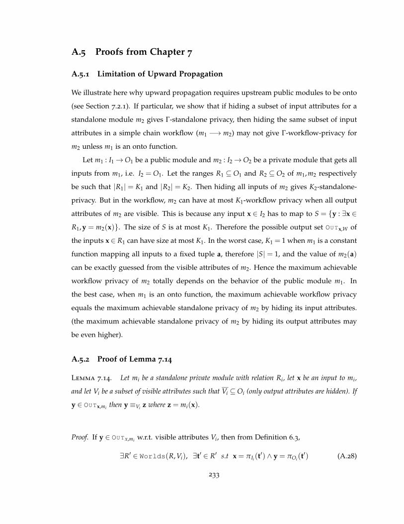
A.5 Proofs from Chapter 7

A.5.1 Limitation of Upward Propagation

We illustrate here why upward propagation requires upstream public modules to be onto

(see Section 7.2.1). If particular, we show that if hiding a subset of input attributes for a

standalone module m2 gives Γ-standalone privacy, then hiding the same subset of input

attributes in a simple chain workflow (m1 −→ m2) may not give Γ-workflow-privacy for

m2 unless m1 is an onto function.

Let m1 : I1→O1 be a public module and m2 : I2→O2 be a private module that gets all

inputs from m1, i.e. I2 = O1. Let the ranges R1 ⊆ O1 and R2 ⊆ O2 of m1,m2 respectively

be such that |R1| = K1 and |R2| = K2. Then hiding all inputs of m2 gives K2-standalone-

privacy. But in the workflow, m2 can have at most K1-workflow privacy when all output

attributes of m2 are visible. This is because any input x ∈ I2 has to map to S = y : ∃x ∈

R1,y = m2(x). The size of S is at most K1. Therefore the possible output set OUTx,W of

the inputs x ∈ R1 can have size at most K1. In the worst case, K1 = 1 when m1 is a constant

function mapping all inputs to a fixed tuple a, therefore |S| = 1, and the value of m2(a)

can be exactly guessed from the visible attributes of m2. Hence the maximum achievable

workflow privacy of m2 totally depends on the behavior of the public module m1. In

the best case, when m1 is an onto function, the maximum achievable workflow privacy

equals the maximum achievable standalone privacy of m2 by hiding its input attributes.

(the maximum achievable standalone privacy of m2 by hiding its output attributes may

be even higher).

A.5.2 Proof of Lemma 7.14

Lemma 7.14. Let mi be a standalone private module with relation Ri, let x be an input to mi,

and let Vi be a subset of visible attributes such that Vi ⊆Oi (only output attributes are hidden). If

y ∈ OUTx,mi then y ≡Vi z where z = mi(x).

Proof. If y ∈ OUTx,mi w.r.t. visible attributes Vi, then from Definition 6.3,

∃R′ ∈ Worlds(R,Vi), ∃t′ ∈ R′ s.t x = πIi(t′) ∧ y = πOi(t

′) (A.28)

233

Further, from Definition 6.1, R′ ∈ Worlds(R,Vi) only if πVi(Ri) = πVi(R′). Hence there

must exist a tuple t ∈ Ri such that

πVi(t) = πVi(t′) (A.29)

Since Vi ⊆ Oi, Ii ⊆ Vi. From (A.29), πIi(t) = πIi(t′) = x. Let z = πOi(t), i.e. z = mi(x).

From (A.29), πVi∩Oi(t) = πVi∩Oi(t′), then πVi∩Oi(z) = πVi∩Oi(y). Tuples y and z are defined

on Oi. Hence from Definition 7.5, y ≡Vi z.

Corollary A.31. For a module mi, and visible attributes Vi such that Vi ⊆ Oi, if two tuples y,z

defined on Oi are such that y ≡Vi z, then also y ≡V z where V is a subset of visible workflows in

the workflow such that V = A \ Hi, and Vi ⊆ Hi.

Proof. Since Vi = Ai \Vi = (Ii ∪Oi) \Vi ⊆Oi, and Vi ⊆ Hi,

Vi ∩Oi = Oi \Vi

⊇ Oi \ Hi

= Oi \ (A \V)

= Oi \V

= Oi ∩V

(A is the set of all attributes).

Since πVi∩Oi(y) = πVi∩Oi(z), and, Vi ∩Oi ⊇ V ∩Oi, πV∩Oi(y) = πV∩Oi(z), i.e., y ≡V

z.

Note. Lemma 7.14 does not use any property of single-predecessor workflows and

also works for general workflows. This lemma will be used again for the privacy theorem

of general workflows (Theorem A.44).

A.5.3 Proof of Lemma 7.12

Definition A.32. Given subsets of attributes P, Q ⊆ A, two tuples p,q defined on P, and a

tuple u defined on Q, FLIPp,q(u) = w is a tuple defined on Q constructed as follows: (i) if

πQ∩P(u) = πQ∩P(p), then w is such that πQ∩P(w) = πQ∩P(q) and πQ\P(w) = πQ\P(w),

234

(ii) else if πQ∩P(u) = πQ∩P(q), then w is such that πQ∩P(w) = πQ∩P(p) and πQ\P(w) =

πQ\P(w), (iii) otherwise, w = u.

The following observations capture the properties of FLIP function.

Observation A.33. 1. If FLIPp,q(u) = w, then FLIPp,q(w) = u.

2. FLIPp,q(FLIPp,q(u)) = u.

3. If P ∩Q = ∅, FLIPp,q(u) = u.

4. FLIPp,q(p) = q,FLIPp,q(q) = p.

5. If πQ∩P(p) = πQ∩P(q), then FLIPp,q(u) = u.

6. If Q = Q1 ∪Q2, where Q1 ∩Q2 = ∅, and if FLIPp,q(πQ1(u)) = w1 and

FLIPp,q(πQ2(u)) = w2, then FLIPp,q(u) = w such that πQ1(w) = w1 and πQ2(w) =

2.

The above definition of flipping will be useful when we consider the scenario where

M does not have any successor. When M has successors, we need an extended definition

of tuple flipping, denoted by EFLIP, as defined below.

Definition A.34. Given subsets of attributes P, Q, R ⊆ A, where two tuples p,q defined on

P ∪ R, a tuple u defined on Q and a tuple v defined on R, EFLIPp,q;v(u) = w is a tuple defined

on Q constructed as follows: (i) if v = πR(p), then w is such that πQ∩P(w) = πQ∩P(q) and

πQ\P(w) = πQ\P(w), (ii) else if v = πR(q), then w is such that πQ∩P(w) = πQ∩P(p) and

πQ\P(w) = πQ\P(w), (iii) otherwise, w = u.

Note that EFLIPp,q;πP∩Q(u)(u) = FLIPp,q(u), where R = P ∩Q.

Observation A.35. 1. If EFLIPp,q;v(u) = w, and u′ is a tuple defined on Q′ ⊆ Q , then

EFLIPp,q;v(u′) = πQ′(w).

Next we prove the lemma assuming the existence of a composite public module M =

C(Vi).

Lemma 7.12. Consider a single-predecessor workflow W; any private module mi in W and

any input x ∈ πIi(R); and any y ∈ OUTx,mi w.r.t. a set of visible attributes Vi. Given a set of

hidden attributes Hi ⊆ A, such that (i) the hidden attributes Vi ⊆ Hi, (ii) only output attributes

235

from Oi are included in Vi (i.e. Vi ⊆Oi), and (iii) every module mj in the public-closure C(Vi) is

UD-safe w.r.t. Aj \ Hi. Then y ∈ OUTx,W w.r.t. visible attributes V = A \ Hi.

Proof. We fix a module mi, an input x to mi and a candidate output y ∈ OUTx,mi for x

w.r.t. visible attributes Vi. Let us refer to the set of public modules in C(Vi) by simply C,

and let us consider the composite module M with the modules in C. By the properties

of single-predecessor workflows, M gets all its inputs from mi and sends its outputs to

zero or more than one private modules. By Lemma 7.16, it suffices to prove the lemma

assuming M is UD-safe w.r.t. Hi, where we denote the inputs and outputs of M by I and

O respectively. Clearly I ⊆ Oi is the subset of output attributes of mi that is input to M,

and the hidden attributes Vi ⊆ I.

However mi can also send (i) its visible outputs to other public modules (these public

modules will have mi as its only predecessor, but these public modules will not have any

public path in undirected sense to M), and it can send (ii) visible and hidden attributes

to other private modules.

We will show that y ∈ OUTx,W w.r.t. visible attributes V = A \ Hi by showing the ex-

istence of a possible world R′ ∈ Worlds(R,V), s.t. if πIi(t) = x for some t ∈ R′, then

πOi(t) = y. Since y ∈ OUTx,mi , by Lemma 7.14, y ≡Vi z where z = mi(x). We consider two

cases separately based on whether M has no successor or at least one private successors.

Case I. First consider the easier case that M does not have any successor, so all

outputs of M belong to the set of final outputs. We redefine the module mi to mi as

follows. For an input u to mi, mi(u) = FLIPy,z(mi(u)). All public modules are unchanged,

mj = mj. All private modules mj 6= mi are redefined as follows: On an input u to mj,

mj(u) = mj(FLIPy,z(u)). The required possible world R′ is obtained by taking the join of

the standalone relations of these mj-s, j ∈ [n].

First note that by the definition of mi, mi(x) = y (since mi(x) = FLIPy,z(mi(x)) =

FLIPy,z(z) = y, from Observation A.33(4)). Hence if πIi(t) = x for some t ∈ R′, then

πOi(t) = y.

Next we argue that R′ ∈ Worlds(R,V). Since R′ is the join of the standalone relations

236

for modules mj-s, R′ maintains all functional dependencies Ij → Oj. Also none of the

public modules are unchanged, hence for any public module mj and any tuple t in R′,

πOj(t) = mj(πIj(t)). So we only need to show that the projection of R and R′ on the visible

attributes are the same.

Let us assume, wlog. that the modules are numbered in topologically sorted order.

Let I0 be the initial input attributes to the workflow, and let p be a tuple defined on I0.

There are two unique tuples t ∈ R and t′ ∈ R′ such that πI1(t) = πI1(t′) = p. Since M does

not have any successor, let us assume that M = mn+1, also wlog. assume that the public

modules in C are not counted in j = 1 to n + 1 by renumbering the modules. Note that

any intermediate or final attribute a ∈ A \ I0 belongs to Oj, for a unique j ∈ [1,n] (since

for j 6= `, Oj ∩O` = φ). So it suffices to show that t, t′ projected on Oj are equivalent w.r.t.

visible attributes for all module j, j = 1 to n + 1.

Let cj,m,cj,m be the values of input attributes Ij and dj,m,dj,m be the values of output

attributes Oj of module mj, in t ∈ R and t′ ∈ R′ respectively on initial input attributes p

(i.e. cj,m = πIj(t), cj,m = πIj(t′), dj,m = πOj(t) and dj,m = πOj(t

′)). We prove by induction

on j = 1 to n that

∀j,1≤ j ≤ n,dj,m = FLIPy,z(dj,m) (A.30)

First we argue that proving (A.30) shows that the join of 〈mi〉1≤i≤n is a possible world

of R w.r.t. visible attributes V. (A) When mj is a private module, note that dj,m and

dj,m = FLIPy,z(dj,m) may differ only on attributes Oj ∩Oi But y≡Vi z, i.e. these tuples are

equivalent on the visible attributes. Hence for all private modules, the t, t′ are equivalent

w.r.t. Oj. (actually for all j 6= i, Oj ∩ Oi = ∅, so the outputs are equal and therefore

equivalent). (B) When mj is a public module, j 6= n + 1, Oj ∩Oi = ∅, hence the values of

t, t′ on Oj are the same and therefore equivalent. (C) Finally, consider M = mn+1 that is

not covered by (A.30). M gets all its inputs from mi. From (A.30),

di,m = FLIPy,z(di,m)

Since y,z,di,m,di,m are all defined on attributes Oi, and input to mn+1, In+1 ⊆Oi,

cn+1,m = FLIPy,z(cn+1,m)

237

Hence cn+1,m ≡V cn+1,m. Since these two inputs of mn+1 are equivalent w.r.t. V, by the

UD-safe property of M = mn+1, its outputs are also equivalent, i.e. dn+1,m ≡V dn+1,m.

Hence the projections of t, t′ on On+1 are also equivalent. Combining (A), (B), (C), t, t′ are

equivalent w.r.t. V.

Proof of (A.30). The base case follows for j = 1. If m1 6= mi (mj can be public or

private), then I1 ∩Oi = ∅, so for all input u,

mj(u) = mj(FLIPy,z(u)) = mj(u)

Since the inputs c1,m = c1,m (both projections of initial input p on I1), the outputs

d1,m = d1,m. This shows (A.30). If m1 = mi, the inputs are the same, and by definition of

m1,

d1,m = m1(c1,m)

= FLIPy,z(mi(c1,m))

= FLIPy,z(mi(c1,m))

= FLIPy,z(d1,m)

This shows (A.30).

Suppose the hypothesis holds until j− 1, consider mj. From the induction hypothesis,

cj,m = FLIPy,z(cj,m), hence cj,m = FLIPy,z(cj,m) (see Observation A.33 (1)).

(i) If j = i, again,

di,m = mi(ci,m)

= FLIPy,z(mi(ci,m))

= FLIPy,z(mi(FLIPy,z(ci,m)))

= FLIPy,z(mi((ci,m))

= FLIPy,z(di,m)

FLIPy,z(ci,m) = ci,m follows due to the fact that Ii ∩Oi = ∅, y,z are defined on Oi,

whereas ci,m is defined on Ii (see Observation A.33 (3)).

238

(ii) If j 6= i and mj is a private module,

dj,m = mj(cj,m)

= mj(FLIPy,z(cj,m))

= mj(cj,m)

= dj,m

= FLIPy,z(dj,m)

FLIPy,z(dj,m) = dj,m follows due to the fact that Oj ∩Oi = ∅, y,z are defined on Oi,

whereas di,m is defined on Oj (again see Observation A.33 (3)).

(iii) If mj is a public module, j ≤ n, mj = mj.

Here

dj,m = mj(cj,m)

= mj(cj,m)

= mj(FLIPy,z(cj,m))

= mj(cj,m)

= dj,m

= FLIPy,z(dj,m)

FLIPy,z(dj,m) = dj,m again follows due to the fact that Oj ∩Oi = ∅. FLIPy,z(cj,m)

= cj,m follows due to following reason. If Ij ∩Oi = ∅, i.e. if mj does not get any

input from mi, again this is true (Observation A.33(3)). If mj gets an input from mi,

i.e. Ij ∩Oi 6= ∅, since mj 6= mn+1, Ij ∩Oi does not include any hidden attributes from

Vi. But y ≡Vi z, i.e. the visible attribute values of y,z are the same. In other words,

πIj∩Oi(y) = πIj∩Oi(z), and from Observation A.33 (5), FLIPy,z(cj,m) = cj,m.

This completes the proof of the lemma for Case-I.

Case II.

Now consider the case when M has one or more private successors (note that M can-

not have any public successor by definition). Let M = mk, and assume that the modules

239

m1, · · · ,mn are sorted in topological order (again, the nodes inside M are not considered

explicitly). Hence I = Ik,O = Ok, and Ik ⊆ Oi. Let wy = M(πIk(y)), wz = M(πIk(z)). In-

stead of y,z, the flip function will be w.r.t. Y,Z, where Y is the concatenation of y and

wy (πOi(Y) = y, πOk(Y) = wy), and Z is the concatenation of z and wz. Hence Y,Z are

defined on attributes Oi ∪Ok.

We redefine the module mi to mi as follows. Note that since input to M, Ik ⊆Oi, Oi is

disjoint union of Ik and Oi \ Ik. For an input u to mi, mi(u), defined on Oi is such that

πOi\Ik(mi(u)) = FLIPY,Z(πOi\Ik

(mi(u)))

and

πIk(mi(u)) = EFLIPY,Z;M(πIk (mi(u)))(πIk(mi(u)))

For the component with EFLIP, in terms of the notations in Definition A.34, R = Ok,

P = Q = Oi. p = Y,q = Z, defined on P ∪ R = Oi ∪ Ok. v = M(πIk(mi(u))), defined

on Ok. u in Definition A.34 corresponds to mi(u). All public modules are unchanged,

mj = mj. All private modules mj 6= mi are redefined as follows: On an input u to mj,

mj(u) = mj(FLIPY,Z(u)). The required possible world R′ is obtained by taking the join of

the standalone relations of these mj-s, j ∈ [n].

First note that by the definition of mi, mi(x) = y due to the following reason:

(i) M(πIk(mi(x))) = M(πIk(z)) = wz = πOk(Z), so

πIk(mi(x)) = EFLIPY,Z;M(πIk (mi(x)))(πIk(mi(x)))

= EFLIPY,Z;M(πIk (z))(πIk(z))

= πIk(y))

(ii)

πOi\Ik(mi(x)) == FLIPY,Z(πOi\Ik

(mi(x)))

= FLIPY,Z(πOi\Ik(z))

= πOi\Ik(y)

Taking union of (i) and (ii), mi(x) = y. Hence if πIi(t) = x for some t ∈ R′, then

πOi(t) = y.

240

Again, next we argue that R′ ∈ Worlds(R,V), and it suffices to show that the projec-

tion of R and R′ on the visible attributes are the same.

Let I0 be the initial input attributes to the workflow, and let p be a tuple defined on

I0. There are two unique tuples t ∈ R and t′ ∈ R′ such that πI1(t) = πI1(t′) = p. Note that

any intermediate or final attribute a ∈ A \ I0 belongs to Oj, for a unique j ∈ [1,n] (since

for j 6= `, Oj ∩O` = φ). So it suffices to show that t, t′ projected on Oj are equivalent w.r.t.

visible attributes for all module j, j = 1 to n + 1.

Let cj,m,cj,m be the values of input attributes Ij and dj,m,dj,m be the values of output

attributes Oj of module mj, in t ∈ R and t′ ∈ R′ respectively on initial input attributes p

(i.e. cj,m = πIj(t), cj,m = πIj(t′), dj,m = πOj(t) and dj,m = πOj(t

′)). We prove by induction

on j = 1 to n that

∀j 6= i,1≤ j ≤ n,dj,m = FLIPY,Z(dj,m) (A.31)

πIk(di,m) = EFLIPY,Z;M(πIk (di,m))(πIk(di,m)) (A.32)

πOi\Ik(di,m) = FLIPY,Z(πOi\Ik

(di,m)) (A.33)

First we argue that proving (A.31), (A.32) and (A.33) shows that the join of 〈mi〉1≤i≤n

is a possible world of R w.r.t. visible attributes V.

(A) When mj is a private module, j 6= i, note that dj,m and dj,m = FLIPY,Z(dj,m) may

differ only on attributes (Ok ∪Oi)∩Oj. But for j 6= i and j 6= k (mj is private module

whereas mk is the composite public module), (Ok ∪ Oi) ∩ Oj = ∅. Hence for all

private modules other than mi, the t, t′ are equal w.r.t. Oj and therefore equivalent.

(B) For mi, from (A.32), πIk(di,m) = EFLIPY,Z;M(πIk (di,m))(πIk(di,m)). Here πIk(di,m) and

πIk(di,m) may differ on Ik only if M(πIk(di,m)) ∈ wy,wz. By Corollary cor:out-

equiv, y ≡V z, i.e. πIk(y) ≡V πIk(z). But since M is UD-safe, by the downstream-

safety property, wy≡V wz. Then by the upstream-safety property, all inputs πIk(di,m)

≡V y ≡V z such that M(πIk(di,m)) ∈ wy,wz. In particular, if M(πIk(di,m)) = wy,

then πIk(di,m) = πIk(z), and πIk(z),πIk(di,m) will be equivalent w.r.t. V. Similarly, if

M(πIk(di,m)) = wz, then πIk(di,m) = πIk(y), and πIk(y),πIk(di,m) will be equivalent

w.r.t. V. So t, t′ are equivalent w.r.t. V ∩ Ik.

241

Next we argue that t, t′ are equivalent w.r.t. V ∩ (Oi \ Ik). From (A.32),

πOi\Ik(di,m) = FLIPY,Z(πOi\Ik

(di,m))

πOi\Ik(di,m) and πOi\Ik

(di,m) differ only if πOi\Ik(di,m) = πOi\Ik

(y), then πOi\Ik(di,m) =

πOi\Ik(z), or, πOi\Ik

(di,m) = πOi\Ik(z), then πOi\Ik

(di,m) = πOi\Ik(y). But πOi\Ik

(y),

πOi\Ik(z) are equivalent w.r.t. visible attributes V. Hence πOi\Ik

(di,m) and πOi\Ik(di,m)

are equivalent w.r.t. V. Hence t, t′ are equivalent on Oi.

(C) When mj is a public module, dj,m = FLIPY,Z(dj,m). Here dj,m,dj,m can differ only on

(Ok ∪Oi)∩Oj. If j 6= k, the intersection is empty, and we are done. If j = k, dj,m,dj,m

may differ only if dj,m ∈ wy,wz. But note that y ≡Vi z, so πIk(y) ≡Vi πIk(z), and

πIk(y)≡V πIk(z). Since mk is UD-safe, for these two equivalent inputs the respective

outputs wy,wz are also equivalent. Hence in all cases the values of t, t′ on Ok are

equivalent.

Combining (A), (B), (C), the projections of t, t′ on Oj are equivalent for all 1 ≤ j ≤ n; i.e.

t, t′ are equivalent w.r.t. V.

Proof of (A.31), (A.32) and (A.33). The base case follows for j = 1. If m1 6= mi (m1 can

be public or private, but k 6= 1 since mi is its predecessor), then I1 ∩ (Oi ∪Ok) = ∅, so for

all input u, mj(u) = mj(FLIPY,Z(u)) = mj(u) (if m1 is private) and mj(u) = mj(u) (if m1 is

public). Since the inputs c1,m = c1,m (both projections of initial input p on I1), the outputs

d1,m = d1,m. This shows (A.31). If m1 = mi, the inputs are the same, and by definition of

m1,

πIk(d1,m) = πIk(m1(c1,m))

= EFLIPY,Z;M(πIk (m1(c1,m)))(πIk(m1(c1,m)))

= EFLIPY,Z;M(πIk (m1(c1,m)))(πIk(m1(c1,m)))

= EFLIPY,Z;M(πIk (d1,m))(πIk(d1,m))

This shows (A.32) for i = 1. Again, by definition of m1,

πO1\Ik(d1,m) = πO1\Ik

(m1(c1,m))

242

= FLIPY,Z(πO1\Ik(m1(c1,m))

= FLIPY,Z(πO1\Ik(m1(c1,m))

= FLIPY,Z(πO1\Ik(d1,m)

This shows (A.33).

Suppose the hypothesis holds until j− 1, consider mj. From the induction hypothesis,

if Ij ∩ Oi = ∅ (mj does not get input from mi) then cj,m = FLIPY,Z(cj,m), hence cj,m =

FLIPY,Z(cj,m) (see Observation A.33(1)).

(i) If j = i, Ii ∩Oi = ∅, hence ci,m = FLIPY,Z(ci,m) = ci,m (Ii ∩ (Oi ∪Ok) = ∅, mk is a

successor of mi, so mi cannot be successor of mk). By definition of mi,

πIk(di,m) = πIk(mi(ci,m))

= EFLIPY,Z;M(πIk (mi(ci,m)))(πIk(mi(ci,m)))

= EFLIPY,Z;M(πIk (mi(ci,m)))(πIk(mi(ci,m)))

= EFLIPY,Z;M(πIk (di,m))(πIk(di,m))

This shows (A.32).

Again,

πOi\Ik(di,m) = πOi\Ik

(mi(ci,m))

= FLIPY,Z(πOi\Ik(mi(ci,m)))

= FLIPY,Z(πOi\Ik(mi(ci,m)))

= FLIPY,Z(πOi\Ik(di,m))

This shows (A.33).

(ii) If j = k, mk gets all its inputs from mi, so πIk(di,m) = ck,m. Hence

ck,m = EFLIPY,Z;M(πIk (di,m))(ck,m)

= EFLIPY,Z;M(ck,m)(ck,m)

= EFLIPY,Z;dk,m(ck,m)

243

Therefore,

dk,m = mk(ck,m)

= mk(ck,m)

= mk(EFLIPY,Z;dk,m(ck,m))

Lets evaluate the term mk(EFLIPY,Z;dk,m(ck,m)). This says that for an input to mk is

ck,m, and its output dk,m, (a) if dk,m = wy, then

EFLIPY,Z;dk,m(ck,m) = πIk(z),

and in turn

dk,m = mk(EFLIPY,Z;dk,m(ck,m)) = wz;

(b) if dk,m = wz, then

EFLIPY,Z;dk,m(ck,m) = πIk(y),

and in turn

dk,m = mk(EFLIPY,Z;dk,m(ck,m)) = wy;

(c) otherwise

dk,m = mk(EFLIPY,Z;dk,m(ck,m))

= mk(ck,m) = dk,m

According to Definition A.32, the above implies that

dk,m = FLIPwy,wz(dk,m)

= FLIPY,Z(dk,m)

This shows (A.31).

244

(iii) If j 6= i and mj is a private module, mj can get inputs from mi. (but since there is

no data sharing Ij ∩ Ik = ∅), and other private or public modules m`,` 6= i (` can be

equal to k). Let us partition the input to mj (cj,m and cj,m defined on Ij) on attributes

Ij ∩Oi and Ij \Oi From (A.31), using the IH,

πIj\Oi(cj,m) = FLIPY,Z(πIj\Oi

(cj,m)) (A.34)

Now Ik ∩ Ij = ∅, since there is no data sharing. Hence (Ij ∩Oi) ⊆ (Oi \ Ik). From

(A.33) using Observation A.35,

πIj∩Oi(cj,m) = FLIPY,Z(πIj∩Oi(cj,m)) (A.35)

From (A.34) and (A.35), using Observation A.33 (6), and since cj,m,cj,m are defined

on Ij, so

cj,m = FLIPY,Z(cj,m) (A.36)

From (A.36),

dj,m = mj(cj,m)

= mj(FLIPY,Z(cj,m))

= mj(cj,m)

= dj,m

= FLIPY,Z(dj,m)

FLIPY,Z(dj,m) = dj,m follows due to the fact that Oj ∩ (Oi ∪Ok) = ∅ (j 6= i,k), Y,Z

are defined on Oi ∪Ok, whereas dj,m is defined on Oj (again see Observation A.33

(3)).

(iv) Finally consider mj is a public module such that j 6= k. mj can still get input from

mi, but none of the attributes in Ij ∩Oi can be hidden by the definition of mk = M =

C(Vi). Further, by the definition of M = mk, mj cannot get any input from mk (M

245

is the closure of public module); so Ij ∩Ok = ∅. Let us partition the inputs to mj

(cj,m and cj,m defined on Ij) into three two disjoint subsets: (a) Ij ∩Oi, and (b) Ij \Oi.

Since there is no data sharing Ik ∩ Ij = ∅, and we again get (A.36) that

cj,m = FLIPY,Z(cj,m)

= cj,m

FLIPy,z(cj,m) = cj,m follows due to following reason. If Ij ∩Oi = ∅, i.e. if mj does not

get any input from mi, again this is true (then Ij ∩ (Oi ∪Ok) = (Ij ∩Oi)∪ (Ij ∩Ok) =

∅). If mj gets an input from mi, i.e. Ij ∩Oi 6= ∅, since j 6= k, Ij ∩Oi does not include

any hidden attributes from Vi (mk is the closure C(Vi)). But y ≡Vi z, i.e. the visible

attribute values of y,z are the same. In other words, πIj∩Oi(y) = πIj∩Oi(z), and again

from Observation A.33 (5),

FLIPY,Z(cj,m) = FLIPy,z(cj,m) = cj,m

(again, Ij ∩Ok = ∅).

Therefore,

dj,m = mj(cj,m)

= mj(cj,m)

= mj(FLIPY,Z(cj,m))

= mj(cj,m)

= dj,m

= FLIPY,Z(dj,m)

FLIPY,Z(dj,m) = dj,m again follows due to the fact that Oj ∩ (Oi ∪Ok) = ∅, since

j /∈ i,k.

Hence all the cases for the IH hold true, and this completes the proof of the lemma for

Case-II.

246

A.5.4 Proof of Lemma 7.16

Lemma 7.16. Let M be a composite module consisting of public modules. Let H be a subset

of hidden attributes such that every public module mj in M is UD-safe w.r.t. Aj \ H. Then M is

UD-safe w.r.t. (I ∪O) \ H.

Proof. Let us assume, wlog., that the modules in M are m2, · · · ,mk where modules are

listed in topological order. For j = 2 to k, let Mj be the composite module comprising

the modules m2, · · · ,mj, and let I j,Oj be its input and output. Hence Mp = M, Ip = I and

Op = O. We prove by induction on 2≤ j ≤ p that Mj is UD-safe w.r.t. H ∩ (I j ∪Oj).

The base case directly follows for j = 2, since A2 = I2∪O2 = I2∪O2. Let the hypothesis

hold until j = j and consider j + 1. Hence Mj is UD-safe w.r.t. (I j ∪Oj) \ H. The module

mj+1 may consume some outputs of Mj (m2 to mj). Hence

I j+1 = I j ∪ Ij+1 \Oj and Oj+1 = Oj ∪Oj+1 \ Ij+1 (A.37)

First we show that for two equivalent inputs the outputs are equivalent. Consider two

inputs x1, x2 to Mj+1 (on attributes I j+1) and let y1 = Mj+1(x1) and y2 = Mj+1(x2) (on

attributes Oj+1).

Let x1 ≡V x2 w.r.t. V = (I j+1 ∪Oj+1) \H. By (A.37), x1 ≡V1 x2 where V2 = (I j ∪Oj) \H.

This is because Oj ∩ I j = ∅ and therefore I j ⊆ I j+1. Since modules are sorted in topological

order, all of the attributes in Oj+1 belong to Oj+1. Also recall that every attribute is

produced by a unique module; hence Oj ∩Oj+1 = ∅. Hence y1 can be partitioned into

y11 and y12, where y11 is defined on Oj+1 and y12 is defined on Oj; let y21,y22 be the

corresponding partitions of y2.

Similarly, let x12 be projections of x1 on I j similarly define x22 for x2. Since x1 ≡V2 x2,

x12 ≡V2 x22. Since y12 = Mj(x12) and y22 = Mj(x22), by IH

y12 ≡V2 y22 (A.38)

Let x′11 (resp. x′21) be projections of x1 (resp. x22) on Ij+1 \Oj. Hence x′11 ≡V x′21. Let

x′′11 (resp. x′′21) be projections of y12 (resp. y22) on Ij+1 ∩Oj. Since y12 ≡V2 y22, x′′11 ≡V2 x′′21.

Let x11 be concatenation of x′11, x′′11; similarly x12. Note that these are defined on Ij+1.

247

V = (I j+1 ∪Oj+1) \ H and V2 = (I j ∪Oj) \ H. Therefore x11 ≡V1 x12, where V1 = (Ij+1 ∪

Oj+1) \ H. Since mj+1 is UD-safe w.r.t. V1,

y11 ≡V1 y21 (A.39)

(note that y11 = mj+1(x11),y21 = mj+1(x21)).

V1 ∪V2 ⊇ V. Hence from (A.38) and (A.39), concatenating y11,y12 to y1 and y21,y22 to

y2,

y1 ≡V y2

This shows that for two equivalent input the outputs are equivalent. The other direction,

for two equivalent outputs all of their inputs are equivalent can be proved in similar way

by considering modules in reverse topological order from mk to m2.

A.5.5 Proof of Proposition 7.11

By Definition 7.8, a workflow W is not a single-predecessor workflow, if one of the fol-

lowing holds: (i) there is a public module mj in W that belongs to the public-closure of a

private module mi but has no directed path from mi, or, (ii) such a public module mj has

directed path from more than one private modules, or, (iii) W has data sharing.

To prove the proposition we provide three example workflows where exactly one of

the violating conditions (i), (ii), (iii) holds, and Theorem 7.10 does not hold in those

workflows.

Case (i) was shown in Section 7.3.2. To complete the proof we demonstrate here

cases (ii) and (iii). We start by considering data sharing and give an example in which

the second condition of Definition 7.8 holds, but in which the propagation only through

public modules does not suffice due to data sharing.

Multiple private predecessor. Finally we give an example where a public module

belonging to a public-closure has more than one private predecessors.

Example A.36. Consider the workflow Wb in Figure A.5a, which is a modification of Wa by

the addition of private module m0, that takes a0 as input and produces a2 = m0(a0) = a0

as output. The public module m3 is in public-closure of m1, but has directed public paths

248

a0 a1 a2 a3 a4 a5 a6

r1 0 0 0 0 0 0 0

r2 1 0 1 0 1 1 1

r3 0 0 1 0 1 1 1

r4 1 1 1 1 1 1 1

Table A.1: Relation Rb for workflow Wb given in Figure A.5a

from both m0 and m1. The relation Rb for Wb in given in Table A.1 where the hidden

attributes a2, a3, a4, a5 are colored in grey.

Now we have exactly the same problem as before: When m1 maps 0 to 1, a5 = 1

irrespective of the value of a4. In the first row a6 = 0, whereas in the second row a6 = 1.

However, whatever the new definitions of m0 are for m0 and m4 for m4, m4 cannot map 1

to both 0 and 1. Hence Γ = 1. 2

(a) m3 has paths from

m0,m1

(b) a3 is shared as in-

put to m2,m3

Figure A.5: White modules are public, Grey are private.

Example A.37. Consider the workflow, say Wd, given in Figure A.5b. All attributes take

values in 0,1. The initial inputs are a1, a2, and final outputs are a6, a7; only m4 is public.

The functionality of modules is as follows: (i) m1 takes a1, a2 as input and produces

m1(a1, a2) = (a3 = a1, a4 = a2). (ii) m2 takes a3, a4 as input and produces a5 = m2(a3, a4) =

a3 ∨ a4 (OR). (iii) m3 takes a5 as input and produces a6 = m3(a5) = a5. (iv) m4 takes a3 as

input and produces a7 = m4(a3) = a3. Note that data a3 is input to both m2,m4, hence the

249

workflow has data sharing.

Now focus on private module m1 = mi. Clearly hiding output a3 of m1 gives 2-

standalone privacy. and for hidden attribute hi = a3, the public-closure C(hi) = m2.

As given in the theorem, Hi ⊆Oi ∪⋃

m`∈M− A` = a3, a4, a5 in this case.

We claim that hiding even all of a3, a4, a5 gives only trivial 1-workflow-privacy of

m1, although the UD-safe condition is satisfied for m2 (actually hiding a3, a4 gives 4-

standalone-privacy for m1). Table A.2 gives the relation Rd, where the hidden attribute

values are in Grey.

a1 a2 a3 a4 a5 a6 a7

r1 0 0 0 0 0 0 0

r2 0 1 0 1 1 1 0

r3 1 0 1 0 1 1 1

r4 1 1 1 1 1 1 1

Table A.2: Relation Rd for workflow Wd given in Figure A.5.

When a3 (and also a4) is hidden, a possible candidate output of input tuple x = (0,0) to

m1 is (1,0). So we need to have a possible world where m1 is redefined as m1(0,0) = (1,0).

Then a5 takes value 1 in the first row, and this is the only row with visible attributes

a1 = 0, a2 = 0. So this requires that m3(a5 = 1) = (a6 = 0) and m4(a3 = 1) = (a7 = 0), to

have the same projection on visible a6, a7.

The second, third and fourth rows, r2,r3,r4, have a6 = 1, so to have the same projection,

we need a5 = 0 for these three rows, so we need m3(a5 = 0) = (a6 = 1) (since we had to

already define m3(1) = 0). When a5 is 0, since the public module m2 is an OR function, the

only possibility of the values of a3, a4 in rows r2,r3,r4 are (0,0). Now we have a conflict on

the value of the visible attribute a7, which is 0 for r2 but 1 for r3,r4, whereas for all these

rows the value of a3 is 0. m4 being a function with dependency a3→ a7, cannot map a3

to both 0 and 1. Similarly we can check that if m1(0,0) = (0,1) or m1(0,0) = (1,1) (both

a3, a4 are hidden), we will have exactly the same problem. Hence all possible worlds of

Rd with these hidden attributes must map m1(0,0) to (0,0), and therefore Γ = 1. 2

250

A.5.6 Proof of Theorem 7.18

Theorem 7.18. Given public module mi with total number of attributes k, and a subset of

attributes V, checking whether mi is UD-safe w.r.t V is coNP-hard in k.

Proof. We do a reduction from UNSAT, where given n variables x1, · · · , xn, and a Boolean

formula f (x1, · · · , xn), the goal is to check whether f is not satisfiable. In our construction,

mi has n+ 1 inputs x1, · · · , xn and y, and the output is z = mi(x1, · · · , xn,y) = f (x1, · · · , xn)∨

y (OR). The set of visible attributes is y,z; so all of x1, · · · , xn are hidden. We claim that

f is not satisfiable if and only if mi is UD-safe w.r.t. V.

Suppose f is not satisfiable, so for all assignments of x1, · · · , xn, f (x1, · · · , xn) = 0.

For output z = 0, then the visible attribute y must have 0 value in all the rows of the

relation of mi. Also for z = 1, the visible attribute y must have 1 value, since in all rows

f (x1, · · · , xn) = 0. Hence for equivalent inputs w.r.t. V, the outputs are equivalent and

vice versa. Therefore mi is UD-safe w.r.t. V.

Now suppose f is satisfiable, then there is at least one assignment of x1, · · · , xn, such

that f (x1, · · · , xn) = 1. In this row, for y = 0, z = 1. However for all assignments of

x1, · · · , xn, whenever y = 1, z = 1. So for output z = 1, all inputs producing z are not

equivalent w.r.t. the visible attribute y, therefore mi is not upstream-safe and hence not

UD-safe.

A.5.7 Communication Complexity Lower Bound for UD-safe Subsets

Given a public module mj and a subset V ⊆ Aj, in this section we give a lower bound on

the communication complexity to verify if V is a UD-safe subset for mj. This also gives a

lower bound for the optimization problem of finding the optimal UD-safe subset for mj:

assume that each attribute in V has cost > 0 whereas all other attributes have cost zero;

then the optimization problem has a solution of cost 0 if and only if V is a UD-safe subset.

If the standalone relation Rj of mj has N rows, we show that deciding whether V is

UD-safe needs Ω(N) time. The argument uses the similar ideas as given in [63] for the

standalone Secure-View problem. Note that simply reading the relation Rj as input

takes Ω(N) time. So the lower bound of Ω(N) does not make sense unless we assume

251

the presence of a data supplier which supplies the tuples of Rj on demand: Given an

assignment x of the input attributes Ij, the data supplier outputs the value y = mj(x)

of the output attributes Oj. The following theorem shows the Ω(N) communication

complexity lower bound in terms of the number of calls to the data supplier; namely, that

(up to a constant factor) one indeed needs to view the full relation.

Lemma A.38. Given module mj and a subset of attributes V, deciding whether mj is UD-safe

w.r.t V requires Ω(N) calls to the data supplier, where N is the number of tuples in the standalone

relation Rj of mj.

Proof. We prove the theorem by a communication complexity reduction from the set dis-

jointness problem: Suppose Alice and Bob own two subsets A and B of a universe U,

|U| = N. To decide whether they have a common element (i.e. A ∩ B 6= φ) takes Ω(N)

communications [115].

We construct the following relation Rj with N + 1 rows for the module mj. mj has

three input attributes: a,b, id and one output attribute y. The attributes a,b and y are

Boolean, whereas id is in the range [1, N + 1]. The input attribute id denotes the identity

of every row in R and takes value i ∈ [1, N + 1] for the i-th row. The module mj computes

the AND function of inputs a and b, i.e., y = a ∧ b.

Row i, i ∈ [1, N], corresponds to element i ∈ U. In row i, value of a is 1 iff i ∈ A;

similarly, value of b is 1 iff i ∈ B. The additional N + 1-th row has aN+1 = 1 and bN+1 = 0.

The goal is to check if visible attributes V = y (with hidden attributes V = id, a,b) is

UD-safe for mj.

Note that if there is a common element i ∈ A ∩ B, then there are two y values in the

table: in the i-th row, 1 ≤ i ≤ n, the value of y = a ∧ b will be 1, whereas, in the N + 1-

th row it is 0. Hence V = id, a,b or V = y is not UD-safe for mj – all inputs are

equivalent, but their outputs are not equivalent, so the downstream-safety property is not

maintained. If there is no such i ∈ A ∩ B, the value of y in all rows i ∈ [1, N + 1] will be

zero, and V = y will be UD-safe.

So V = y is UD-safe if and only if the input sets are not disjoint. Hence we need to

look at Ω(N) rows to decide whether V = y is UD-safe.

This proof also shows the lower bound for verifying if a subset is downstream-safe.

252

A.5.8 Upper Bound to Find All UD-safe Solutions

The lower bounds studied for the second step of the four step optimization show that

for a public module mj, it is not possible to have poly-time algorithms (in |Aj|) even to

decide if a given subset V ⊆ Aj is UD-safe, unless P = NP. Here we present Algorithm 10

that finds all UD-safe solutions of mj is time exponential in k j = |Aj|, assuming that the

maximum domain size of attributes ∆ is a constant.

Time complexity. The outer for loop runs for all possible subsets of Aj, i.e. 2k j

times. The inner for loop runs for maximum ∆|Ij∩V| times (this is the maximum num-

ber of such tuples x+), whereas the check if V is a valid downstream-safe subset takes

O(∆|Ij\V|) time. Here we ignore the time complexity to check equality of tuples which

will take only polynomial in |Ai| time and will be dominated by the exponential terms.

For the upstream-safety check, the number of 〈x+,y+〉 pairs are at most ∆|Ij∩V|, and to

compute the distinct number of x+,y+ tuples from the pairs can be done in O(∆2|Ij∩V|)

time by a naive search; the time complexity can be improved by the use of a hash function.

Hence the total time complexity is dominated by 2k j ×O(∆|Ij∩V|) ×O(∆|Ij\V| + ∆2|Ij∩V|)

= O(2k j ∆3kj) = O(24k j). By doing a tighter analysis, the multiplicative factor in the expo-

nents can be improved, however, we make the point here that the algorithm runs in time

exponential in k j = |Aj|.

Correctness. The following lemma proves the correctness of Algorithm 10.

Lemma A.39. Algorithm 10 adds V ⊆ Aj to UD− sa f ej if and only if mj is UD-safe w.r.t. V.

Proof. (if) Suppose V is a UD-safe subset for mj. Then V is downstream-safe, i.e. for

equivalent inputs w.r.t. the visible attributes Ij ∩ V, the projection of the output on the

visible attributes Oj ∩V will be the same, so V will pass the downstream-safety test.

Since V is UD-safe, V is also upstream-safe. Clearly, by definition, n1 ≥ n2. Suppose

n1 > n2. Then there are two x+1 and x+2 that pair with the same y+. By construction,

x+1 and x+2 (and all input tuples x to mj that project on these two tuples) have different

value on the visible input attributes Ij ∩ V, but they map to outputs y-s that have the

same value on visible output attributes Oj ∩ V. Then V is not upstream-safe, which is a

contradiction. Hence n1 = n2, and V will also pass the test for upstream-safety and be

253

Algorithm 10 Algorithm to find all UD-safe solutions UD− sa f ej for a public module mj

1: – Set UD− sa f ej = ∅.

2: for every subset V of Aj do

3: /* Check if V is downstream-safe */

4: for every assignment x+ of the visible input attributes in Ij ∩V do

5: –Check if for every assignment x− of the hidden input attributes in Ij \V, whether

the value of πOj∩V(mj(x)) is the same, where πIj∩V(x) = x+ and πIj\V(x) = x−

6: if not then

7: – V is not downstream-safe. Go to the next V.

8: else

9: – V is downstream-safe. Let y+ = πOj∩V(mj(x)) = projection of all such tuples

that have projection = x+ on the visible input attributes

10: – Label this set of input-output pairs (x,mj(x)) by 〈x+,y+〉.

11: end if

12: /* Check if V is upstream-safe */

13: – Consider the pairs 〈x+,y+〉 constructed above. Let n1 be the number of distinct

x+ values, and let n2 be the number of distinct y+ values

14: if n1 == n2 then

15: – V is upstream-safe. Add V to UD− sa f ej.

16: else

17: – V is not upstream-safe. Go to the next V.

18: end if

19: end for

20: end for

21: return The set of subsets UD− sa f ej.

included in UD− sa f ej.

(only if) Suppose V is not UD-safe, then it is either not upstream-safe or not downstream-

safe. Suppose it is not downstream-safe. Then for at least one assignment x+, the values

of y generated by the assignments x− will not be equivalent w.r.t. the visible output

254

attributes, and the downstream-safety test will fail.

Suppose V is downstream-safe but not upstream-safe. Then there are Then there are

two x+1 and x+2 that pair with the same y+. This makes n1 > n2, and the upstream-safety

test will fail.

A.5.9 Proof of Lemma 7.20

The following proposition will be useful to prove the lemma.

Proposition A.40. For a public module mj, for two UD-safe sets U1,U2 ⊆ Aj, if U1 ∩Oj =

U2 ∩Oj, then U1 = U2.

Proof. Assume the contradiction, and wlog. assume that there is an attribute a ∈U1 \U2.

UD-safe condition says that if the inputs to mj are equivalent then the corresponding

outputs are also equivalent w.r.t. the visible attributes and vice versa. Let U1 be the

set visible attributes. This allows us to partition the set of outputs into K equivalence

classes Y1, · · · ,YK, and the set of inputs into K equivalent classes X1, · · · , XK w.r.t. the

same projection on input attribute values, such that for all 1≤ ` ≤ K,

Y` = y = mj(x) : x ∈ X`

Again for visible attributes U2, since U1 ∩Oj = U2 ∩Oj, the set of outputs can be parti-

tioned into the same K equivalence classes Y1, · · · ,YK, and the set of inputs into K equiv-

alent classes Z1, · · · , ZK w.r.t. the same projection on input attribute values, such that for

all 1≤ ` ≤ K,

Y` = y = mj(x) : x ∈ Z`

Hence

y : ∃x ∈ X`,mj(x) = y = y : ∃x ∈ Z`,mj(x) = y

and

X` = Z`

for all 1 ≤ ` ≤ K. Suppose not, and wlog. there is a x ∈ X`, i.e. mj(x) ∈ Y`. Suppose

x /∈ Z`, i.e. mj(x) /∈ Y` which is a contradiction.

255

For all `, X` = Z`. Consider any tuple x ∈ X`. Since a ∈U1 \U2, and both U1,U2 ⊆ Aj,

a ∈U2 \U1. Consider two tuples x1,x2 ∈ Z`, such that πa(x1) 6= πa(x2). Since a is hidden

for U2, two such tuples must exist. But a is visible in U1, and for all tuples in the same

group X`, value of a must be the same (the reverse is not necessarily true). In other

words, since the value of a is different, x1,x2 must belong to different groups w.r.t. U1.

But we argued that X` = Z`, so these two tuples belong to the same group. This is a

contradiction, and therefore no such a, and U1 ⊆ U2. By the same argument, U2 ⊆ U1,

and therefore U1 = U2.

Lemma 7.20. For 1 ≤ j ≤ k, the entry Q[j,`], 1 ≤ ` ≤ pj, stores the minimum cost of the

hidden attributes ∪jx=1Ax ⊇ H j` ⊇ Si∗ such that Aj \ H j` = Uj`, and every module mx,1≤ x ≤ j

in the chain is UD-safe w.r.t. Ax \ H j`.

Proof. We prove this by induction from j = 1 to k. The base case follows by the definition

of Q[1,`], for 1 ≤ ` ≤ p1. Here the requirements are A1 ⊇ H1` ⊇ Si∗, and A1 \ H1` = U1`,

i.e. U1` = H1`. So we set the cost at Q[1,`] to c(U1`) = c(H1`), if U1` ⊇ Si∗.

Suppose the hypothesis holds until j − 1, and consider j. Let H j` be the minimum

solution s.t. Aj \ H j` = Uj` and satisfies the other conditions of the lemma.

First consider the case when there is no q such that Uj−1,q ∩Oj−1 = Uj,` ∩ Ij, where we

set the cost to be ∞. If there is no such q. i.e. for all q≤ pj−1, Uj−1,q ∩Oj−1 6= Uj,` ∩ Ij, then

clearly there cannot be any solution H j` that contains Uj,` and also guarantees UD-safe

properties of all x < j (in particular for x = j− 1). In that case the cost of the solution is

indeed ∞.

Otherwise (when such a q exists), let us divide the cost of the solution c(H j`) into two

disjoint parts:

c(H j`) = c(H j` ∩Oj) + c(H j` \Oj)

We argue that c(Oj ∩ H j`) = c(Oj ∩Uj`). Aj \ H j` = U j`. So Uj` = Aj \Uj` = Aj ∩ H j`.

Then Oj ∩Uj` = Oj ∩ Aj ∩ H j` = Oj ∩ H j`, since Oj ⊆ Aj. Hence c(Oj ∩ H j`) = c(Oj ∩Uj`).

This accounts for the cost of the first part of Q[j,`].

Next we argue that c(H j` \ Oj) = minimum cost Q[j − 1,q], 1 ≤ q ≤ pj, where the

minimum is over those those q where Uj−1,q ∩Oj−1 = Uj,` ∩ Ij. Due to the chain structure

256

of CW , Oj ∩⋃j−1

x=1 Aj = ∅, and Oj ∪⋃j−1

x=1 Ax =⋃j

x=1 Ax. Since ∪jx=1Ax ⊇ H j`, H j` \Oj =

H j` ∩⋃j−1x=1 Ax.

Consider H′ = H j` ∩ ⋃j−1x=1 Ax. By definition of H j`, H′ must satisfy the UD-safe re-

quirement of all 1≤ x ≤ j− 1. Further,⋃j−1

x=1 Ax ⊇ H′. Aj \ H j` = Uj,`, hence

Uj,` = Aj \Uj,` = Aj ∩ H j` ⊆ Hj`

We are considering the case where there is a q such that

Uj−1,q ∩Oj−1 = Uj,` ∩ Ij (A.40)

and therefore

Uj−1,q ∩Oj−1 ⊆Uj,` ⊆ H j`

We claim that if q satisfies (A.40), then Aj−1 \ H′ = Uj−1,q. Therefore, by IH, Q[j − 1,`]

stores the minimum cost solution H′ that includes Uj−1,q, and part of the the optimal

solution cost c(H j` \Oj) for mj is the minimum value of such Q[j− 1,q].

So it remains to show that Aj−1 \ H′ = Uj−1,q. Aj−1 \ H′ = Aj−1 \ H j` ∈ UD− sa f ej−1,

since H j` gives UD-safe solution for mj−1. Suppose Aj−1 \ H j` = Uj−1,y.

Next we argue that Uj−1,q = Uj−1,y, which will complete the proof. Uj−1,y ∩Oj−1 =

(Aj−1 \Uj−1,y) ∩Oj−1 = (Aj−1 ∩ H j`) ∩Oj−1 = H j`) ∩Oj−1, = H j` ∩ Ij = (Aj \Uj,`) ∩ Ij i.e.

Uj−1,y ∩Oj−1 = Uj,` ∩ Ij (A.41)

From (A.40) and (A.41),

Uj−1,q ∩Oj−1 = Uj−1,y ∩Oj−1

, since both Uj−1,q,Uj−1,y ∈ UD − sa f ej−1, from Proposition A.40, Uj−1,q = Uj−1,y. This

completes the proof of the lemma.

A.5.10 Optimal Algorithm for Tree Workflows

Theorem 7.21. The single-subset problem can be solved in PTIME (in n, |A| and L) for tree

workflows.

Proof. Similar to the proof of Theorem 7.19, to obtain an algorithm of time polynomial in

L, for a given module mi, we can go over all choices of safe subsets Si` ∈ Si of mi, compute

257

the public-closure C(Si`), and choose a minimal cost subset Hi = Hi(Si`) that satisfies the

UD-safe properties of all modules in the public-closure. Then, output, among them, a

subset having the minimum cost. Consequently, it suffices to explain how, given a safe

subset Si` ∈ Si, one can solve, in PTIME, the problem of finding a minimum cost hidden

subset Hi that satisfies the UD-safe property of all modules in a subgraph formed by a

given C(Si`).

To simplify notations, the given safe subset Si` will be denoted below by Si∗, the

closure C(Si`) will be denoted by T′, and the output hidden subset will be denoted by H.

Our PTIME algorithm uses dynamic programming to find the optimal H.

First note that since T′ is the public-closure of (some) output attributes for a tree

workflow, T′ is a collection of trees all of which are rooted at the private module mi. Let

us consider the tree T rooted at mj with the subtrees in T′, (note that mi can have private

children that are not considered in T). Let k be the number of modules in T, and the

modules in T be renumbered as mi,m1, · · · ,mk, where the private module mi is the root,

and the rest are public modules.

Now we solve the problem by dynamic programming as follows. Let Q be an k× L

two-dimensional array, where Q[j,`], 1 ≤ j ≤ k,1 ≤ ` ≤ pj denotes the cost of minimum

cost hidden subset H j` that (i) satisfies the UD-safe condition for all public modules in

the subtree of T rooted at mj, that we denote by Tj; and, (ii) Aj \ H j` = Uj`. Here Aj is the

attribute set of mj); the actual solution can be stored easily by standard argument. The

algorithm is described below.

• Initialization for leaf nodes. The initialization step handles all leaf nodes mj in T.

For a leaf node mj, 1≤ ` ≤ pj,

Q[j,`] = c(Uj,`)

• Internal nodes. The internal nodes are considered in a bottom-up fashion (by a

post-order traversal), and Q[j,`] is computed for a node mj after its children are

processed.

For an internal node mj, let mi1 , · · · ,mix be its children in T. Then for 1≤ ` ≤ pj,

1. Consider UD-safe subset Uj,`.

258

2. For y = 1 to x, let Uy = Uj,` ∩ Iiy (intersection of Uj,` with the inputs of miy ).

Since there is no data sharing, Uy-s are disjoint

3. For y = 1 to x,

ky = argminkQ[iy,k] where the minimum is over

1≤ k ≤ piy s.t. Uiy,k ∩ Iiy = Uy

= ⊥ (undefined), if there is no such k

4. Q[j,`] is computed as follows.

Q[j,`] = ∞ if ∃y,1≤ y ≤ x, ky =⊥

= c(Ij ∩Uj`) +x

∑y=1

Q[iy,ky] (otherwise)

• Final solution for Si∗. Now consider the private module mi that is the root of

T. Recall that we fixed a safe solution Si∗ for doing the analysis. Let mi1 , · · · ,mix

be the children of mi in T (which are public modules). Similar to the step before,

we consider the min-cost solutions of its children which exactly match the hidden

subset Si∗ of mi.

1. Consider safe subset Si∗ of mi.

2. For y = 1 to x, let Sy = Si∗ ∩ Iiy (intersection of Si∗ with the inputs of miy ). Since

there is no data sharing, again, Sy-s are disjoint

3. For y = 1 to x,

ky = argminkQ[iy,k] where the minimum is over

1≤ k ≤ piy s.t. Uiy,k ∩ Iiy ⊇ Sy

= ⊥ (undefined), if there is no such k

4. The cost of the optimal H (let us denote that by c∗) is computed as follows.

c∗ = ∞ if ∃y,1≤ y ≤ x, ky =⊥

=x

∑y=1

Q[iy,ky] (otherwise)

259

It is not hard to see that the trivial solution of UD-safe subsets that include all at-

tributes of the modules gives a non-infinite cost solution by the above algorithm.

The following lemma (whose proof is given later) shows that Q[j,`] correctly stores the

desired value. Then the optimal solution H has cost min1≤`≤pk Q[k,`]; the corresponding

solution H can be found by standard procedure.

Lemma A.41. For 1 ≤ j ≤ k, let Tj be the subtree rooted at mj and let Attj =⋃

mq∈TjAq the

entry Q[j,`], 1 ≤ ` ≤ pj, stores the minimum cost of the hidden attributes H j` ⊆ Attj such that

Aj \ H j` = Uj`, and every module mq ∈ Tj, is UD-safe w.r.t. Aq \ H j`.

Given this lemma, the correctness of the algorithm easily follows. For hidden subset

H ⊇ Si∗ in the closure, for every public child miy of mi, H ∩ Iiy ⊇ Si∗ ∩ Iiy = Sy. Further,

each such miy has to be UD-safe w.r.t. H j`. In other words, for each miy , H ∩ Iiy must equal

Uiy,ky for some 1≤ ky ≤ piy . The last step in our algorithm (that computes c∗) tries to find

such a ky that has the minimum cost Q[iy,ky], and the total cost c∗ of H is ∑miyQ[iy,ky]

where the sum is over all children of mi in the tree T (the trees rooted at miy are disjoint,

so the c∗ is sum of those costs).

To complete the proof of Theorem 7.21, we need to prove Lemma A.41, that we prove

the next.

Proof of Lemma A.41

Proof. We prove the lemma by an induction on all nodes at depth h = H down to 1 of the

tree T, where depth H contains all leaf nodes and depth 1 contains the children of the

root mi (which is at depth 0).

First consider any leaf node mj at height H. Then Tj contains only mj and Attj = Aj.

For any 1 ≤ ` ≤ pj, since Attj = Aj ⊇ H j` and Aj \ H j` = Uj,`. hence H j` = Uj,`. In this

case H j` is unique and Q[j,`] correctly stores c(Uj,`) = c(H j`).

Suppose the induction holds for all nodes up to height h + 1, and consider a node mj

at height h. Let mi1 , · · · ,mix be the children of mj which are at height h + 1. Let H j` be the

min-cost solution, which is partitioned into two disjoint component:

c(H j`) = c(H j` ∩ Ij) + c(H j` \ Ij)

260

First we argue that c(H j` ∩ Ij) = c(Uj,`). Aj \ H j` = U j`. So Uj` = Aj \Uj` = Aj ∩ H j`.

Then Ij ∩Uj` = Ij ∩ Aj ∩ H j` = Ij ∩ H j`, since Ij ⊆ Aj. Hence c(Ij ∩ H j`) = c(Ij ∩Uj`). This

accounts for the cost of the first part of Q[j,`].

Next we analyze the cost c(H j` \ Ij). This cost comes from the subtrees Ti1 , · · · , Tix

which are disjoint due to the tree structure and absence of data-sharing. Let us partition

the subset H j` \ Ij into disjoint parts (H j` \ Ij) ∩ Attiy , 1 ≤ y ≤ x. We claim that c((H j` \

Ij) ∩ Attiy) = Q[iy,ky], 1 ≤ y ≤ x, where ky is computed as in the algorithm. This will

complete the proof of the lemma.

Proof of claim: c((H j` \ Ij)∩ Attiy) = Q[iy,ky], 1≤ y≤ x. Let H′ = (H j` \ Ij)∩ Attiy .

Clearly, Attiy ⊇ H′. Since every mq ∈ Tj is UD-safe w.r.t. Aq \ H j`. If also mq ∈ Tiy , then

Aq \ H′ = Aq \ H j`, and therefore all mq ∈ Tiy are also UD-safe w.r.t. H′. In particular, miy

is UD-safe w.r.t. H′, and therefore Aiy \ H′ = Uiy,ky , since Uiy,ky was chosen as the UD-safe

set by our algorithm.

Finally we argue that c(H′) = c(Hiy,ky), where Hiy,ky

is the min-cost solution for miy

among all such subsets. This easily follows from our IH, since miy is a node at depth

h + 1. Therefore, c(H′) = c(Hiy,ky) = Q[iy,ky], i.e.

c((H j` \ Ij) ∩ Attiy) = Q[iy,ky]

as desired. This completes the proof of the lemma.

A.5.11 Proof of Theorem 7.22

Theorem 7.22. The problem of testing whether the single-subset problem has a solution with cost

smaller than a given bound is NP-complete when the public-closure forms an arbitrary subgraph.

This is the case even when both number of attributes and the number of safe and UD-safe subsets

of the individual modules is bounded by a (small) constant.

Proof. Given a CNF formula ψ on n variables z1, · · · ,zn and m clauses ψ1, · · · ,ψm, we

construct a graph as shown in Figure A.6. Let variable zi occurs in mi different clauses

(as positive or negative literals). In the figure, the module p0 is the single-private module

261

Figure A.6: Reduction from 3SAT. Module p0 is private, the rest are public. The narrow

dark edges (in red) denote TRUE assignment, the bold dark edges (in blue) denote FALSE

assignment.

(mi), having a single output attribute a. The rest of the modules are the public modules

in the public-closure C(a).

For every variable zi, we create mi + 2 nodes: pi,yi and xi,1, · · · , xi,mi . For every clause

ψj, we create 2 modules Cj and f j.

The edge connections are as follows:

1. p0 sends its single output a to p1.

2. For every i = 1 to n− 1, pi has two outputs; one is sent to pi+1 and the other is sent

to yi. pn sends its single output to yn.

3. Each yi, i = 1 to n, sends two outputs to xi,1. The blue outgoing edge from yi de-

notes positive assignment of the variable zi, whereas the red edge denotes negative

assignment of the variable zi.

4. Each xi,j, i = 1 to n, j = 1 to mi − 1, sends two outputs (blue and red) to xi,j+1. In

addition, if xi,j, i = 1 to n, j = 1 to mi sends a blue (resp. red) edge to clause node

Ck if the variable zi is a positive (resp. negative) in the clause Ck (and Ck is the j-th

such clause containing zi).

262

5. Each Cj, j = 1 to m, sends its single output to f j.

6. Each f j, j = 1 to m− 1, sends its single output to f j+1, fm outputs the single final

output.

The UD-safe sets are defined as follows:

1. For every i = 1 to n− 1, pi has a single UD-safe set: hide all its inputs and outputs.

2. Each yi, i = 1 to n, has three UD-safe choices: (1) hide its unique input and blue

output, (2) hide its unique input and red output, (3) hide its single input and both

blue and red outputs.

3. Each xi,j, i = 1 to n, j = 1 to mi, has three choices: (1) hide blue input and all blue

outputs, (2) hide red input and all red outputs, (3) hide all inputs and all outputs.

4. Each Cj, j = 1 to m, has choices: hide the single output and at least of the three

inputs.

5. Each f j, j = 1 to m, has the single choice: hide all its inputs and outputs.

Cost. The outputs from yi, i = 1 to n has unit cost, the cost of the other attributes is

0.

The claim is that there is a solution of single-module problem of cost = n if and

only if the 3SAT formula ψ is satisfiable.

(if) Suppose the 3SAT formula is satisfiable, so there is an assignment of the variables

zi that makes Ψ true. If zi is set to True (resp False), choose the blue (resp. red) outgoing

edge from yi. Then choose the other edges accordingly: (1) choose outgoing edge from

p0, (2) choose all input and outputs of pi, i = 1 to n; (3) if blue (resp. red) input of xi,j is

chosen, all its blue (resp. red) outputs are chosen; and, (4) all inputs and outputs of f j are

chosen. Clearly, all these are UD-safe sets by construction.

So we have to only argue about the clause nodes Cj. Since ψ is satisfied by the given

assignment, there is a literal zi ∈ Cj (positive or negative), whose assignment makes it

263

true. Hence at least one of the inputs to Cj will be chosen. So the UD-safe requirements

of all the UD-safe clauses are satisfied. The total cost of the solution is n since exactly one

output of the yi nodes, i = 1 to n, have been chosen.

(only if) Suppose there is a solution to the single-module problem of cost n. Then each

yi can choose exactly one output (at least one output has to be chosen to satisfy UD-safe

property for each yi, and more than one output cannot be chosen as the cost is n). If yi

chooses blue (resp. red) output, this forces the xi,j nodes to select the corresponding blue

(resp. red) inputs and outputs. No xi,j can choose the UD-safe option of selecting all its

inputs and outputs as in that case finally yi be forced to select both outputs which will

exceed the cost. Since Cj satisfies UD-safe condition, this in turn forces each Cj to select

the corresponding blue (resp. red) inputs.

If the blue (resp. red) output of yi is chosen, the variable is set to True (resp. False).

By the above argument, at least one such red or blue input will be chosen as input to each

Cj, that satisfies the corresponding clause ψj.

A.5.12 General Workflows

In this section we discuss the privacy theorem for general workflows as outlined in Sec-

tion 7.5.

First we define directed-path and downward-closure as follows (similar to public path

and public-closure )

Definition A.42. A module m1 has a directed path to another module m2, if there are modules

mi1 ,mi2 , · · · ,mij such that mi1 = m1, mij = m2, and for all 1≤ k < j, Oik ∩ Iik+1 6= ∅.

An attribute a ∈ A has a directed path from to module mj, if there is a module mk such that

a ∈ Ik and mk has a directed path to mj.

Definition A.43. Given a private module mi and a set of hidden output attributes hi ⊆Oi of mi,

the downward-closure of mi w.r.t. hi, denoted by D(hi), is the set of modules mj (both private

and public) such that there is a directed path from some attribute a ∈ hi to mj.

The goal of this section is to prove the following theorem:

264

Theorem A.44. (Privacy Theorem for General workflows) Let W be any workflow. For a

private module mi in W, let Vi be a safe subset for Γ-standalone-privacy s.t. only output attributes

of mi are hidden (i.e. Vi ⊆Oi). Let D(Vi) be the downward-closure of mi w.r.t. hidden attributes

Vi. Let Hi be a set of hidden attributes s.t. Vi ⊆ Hi ⊆Oi ∪⋃

k∈D(Vi)Ak and where for every module

mj ∈ D(Vi) (mj can be private or public), mj is downstream-safe (D-safe) w.r.t. Aj \ Hi. Then the

workflow W is Γ-private w.r.t the set of visible attributes V = A \ (⋃i∈M− Hi).

In the proof of Theorem 7.10 from Lemma 7.12 used the fact that for single-predecessor

workflows, for two distinct private modules mi,mk, the public-closures and the hidden

subsets Hi, Hj are disjoint. However, it is not hard to see that this is not the case for general

workflows, where the downward-closure and the subsets Hi may overlap. Further, the

D-safe property is not monotone (hiding more output attributes will maintain the D-safe

property, but hiding more input attributes may destroy the D-safe property). So we need

to argue that the D-safe property is maintained when we take union of Hi sets in the

workflow. The following proposition will be helpful to prove the privacy theorem for

general workflows.

Lemma A.45. If a module mj is D-safe w.r.t. sets V1,V2 ⊆ Aj, then mj is D-safe w.r.t. V =

V1 ∩V2.

Proof. (Sketch) Given two equivalent inputs x1 ≡V x2 w.r.t. V = V1 ∩V2, we have to show

that their outputs are equivalent: mj(x1) ≡V mj(x2). Even if x1,x2 are equivalent w.r.t. V,

they may not be equivalent w.r.t. V1 or V2. In the proof we construct a new tuple x3 such

that x1 ≡V1 x3, and x2 ≡V2 x3. Then using the D-safe properties of V1 and V2, we show that

mj(x1) ≡V mj(x3) ≡V mj(x2).

The full proof is given in Appendix A.5.13.

Along with this lemma, two other simple observations will be useful.

Observation A.46. 1. Any module mj is D-safe w.r.t. Aj (hiding nothing maintains

downstream-safety property).

2. If mj is D-safe w.r.t. V, and if V ′ is such that V ′ ⊆ V, but V ′ ∩ Ij = V ∩ Ij, then mj

is also D-safe w.r.t. V ′ (hiding more output attributes maintains downstream-safety

property).

265

Proof of Theorem A.44. Using Lemma A.47 and Lemma A.45, we present the proof of

Theorem A.44 below.

Proof. We again argue that if Hi satisfies the conditions in Theorem A.44, then H′i =⋃`∈M− H` satisfies the conditions in Lemma A.47. The first two conditions are easily

satisfied by H′i : (i) Vi ⊆ Hi ⊆⋃

`∈M− H` = H′i ; (ii) Vi ⊆Oi is unchanged.

Now we argue that (iii) every module mj in the downward-closure D(Vi) is D-safe

w.r.t. H′i . From the conditions in the theorem, each module mj ∈ D(Vi) is D-safe w.r.t.

Aj \ Hi. We show that for any other private module mk 6= mi, mj is also D-safe w.r.t.

Aj \ Hk. There may be three such cases as discussed below.

Case-I: If mj ∈ D(Vk), by the D-safe conditions in the theorem, mj is D-safe w.r.t.

Aj \ Hk.

Case-II: If mj /∈ D(Vk) and mj 6= mk, for any private module mk 6= mi, then Aj ∩

Hk = ∅ (since Hk ⊆ Ok ∪⋃

`∈D(Vk)A` from the theorem). Hence Aj \ Hk = Aj, and from

Observation A.46, mj is D-safe w.r.t. Aj \ Hk.

Case-III: If mj /∈D(Vk) but mj = mk (or j = k), then Hk ∩Aj⊆Oj (again since Hk⊆Ok ∪⋃`∈D(Vk)

A` and Ok =Oj). From Observation A.46, mj is UD-safe w.r.t. Aj, and Aj \Hk⊆ Aj

is such that Aj ∩ Ij = Ij = (Aj \ Hk)∩ Ij. Then again from the same observation, mj is UD-

safe w.r.t. Aj \ Hk.

Hence mj is D-safe w.r.t. Aj \ Hi and for all mk ∈ M−, mk 6= mi, mj is D-safe w.r.t.

Aj \ Hk. By Lemma A.45, then mj is D-safe w.r.t. (Aj \ Hi) ∩ (Aj \ Hk) = Aj \ (Hi ∪ Hk).

(this is by the simple fact that (Aj \ Hi)∩ (Aj \ Hk) = (Aj ∩ Hi)∩ (Aj ∩ Hk) = Aj ∩ Hi ∪ Hk

= Aj \ (Hi ∪ Hj)). By a simple induction on all k ∈M−, mj is D-safe w.r.t. Aj \ (⋃

k∈M−)Hk

= Aj \ H′i . Hence H′i satisfies the conditions stated in the lemma. The rest of the proof

follows by the same argument as in the proof of Theorem 7.10.

Now the proof can be completed using exactly the same argument as in Theorem 7.10.

Theorem A.44 also states that each private module mi is Γ-standalone-private w.r.t. visible

attributes Vi, i.e., |OUTx,mi | ≥ Γ for all input x to mi, for i ∈ M− (see Definition 6.3). From

Lemma 7.12, using H′i in place of Hi, this implies that for all input x to private modules

mi, |OUTx,W | ≥ Γ w.r.t V = A \ H′i = A \ ⋃`∈M− H`. From Definition 6.6, this implies that

each mi ∈ M− is Γ-workflow-private w.r.t. V = A \⋃i∈M− Hi; equivalently W is Γ-private

266

w.r.t. V.

Again, similar to Lemma 7.12, we present the following lemma that allows us to

analyze every private module separately to prove Theorem A.44.

Lemma A.47. Consider any workflow W; any private module mi in W and any input x ∈ πIi(R);

and any y ∈ OUTx,mi w.r.t. a set of visible attributes Vi. Given a set of hidden attributes Hi ⊆ A,

such that (i) the hidden attributes Vi ⊆ Hi, (ii) only output attributes from Oi are included in Vi

(i.e. Vi ⊆ Oi), and (iii) every module mj (private or public) in the downward-closure D(Vi) is

D-safe w.r.t. Aj \ Hi. Then y ∈ OUTx,W w.r.t. visible attributes V = A \ Hi.

Proof. We fix a module mi, an input x to mi and a candidate output y ∈ OUTx,mi for x w.r.t.

visible attributes Vi. for simplicity, let us refer to the set of modules in D(Vi) by D. We

will show that y ∈ OUTx,W w.r.t. visible attributes V = A \ Hi by showing the existence

of a possible world R′ ∈ Worlds(R,V), s.t. if πIi(t) = x for some t ∈ R′, then πOi(t) = y.

Since y ∈ OUTx,mi , by Lemma 7.14, y ≡Vi z where z = mi(x).

We will use the FLIP function used in the proof of Lemma 7.12 (see Appendix A.5.3).

We redefine the module mi to mi as follows. For an input u to mi, mi(u) = FLIPy,z(mi(u)).

All other public and private modules are unchanged, mj = mj. The required possible

world R′ is obtained by taking the join of the standalone relations of these mj-s, j ∈ [n].

First note that by the definition of mi, mi(x) = y (since mi(x) = FLIPy,z(mi(x)) =

FLIPy,z(z) = y, from Observation A.33). Hence if πIi(t) = x for some t ∈ R′, then πOi(t) =

y.

Next we argue that R′ ∈ Worlds(R,V). Since R′ is the join of the standalone relations

for modules mj-s, R′ maintains all functional dependencies Ij → Oj. Also none of the

public modules are unchanged, hence for any public module mj and any tuple t in R′,

πOj(t) = mj(πIj(t)). So we only need to show that the projection of R and R′ on the visible

attributes are the same.

Let us assume, wlog. that the modules are numbered in topologically sorted order.

Let I0 be the initial input attributes to the workflow, and let p be a tuple defined on I0.

There are two unique tuples t ∈ R and t′ ∈ R′ such that πI1(t) = πI1(t′) = p. Note that

any intermediate or final attribute a ∈ A \ I0 belongs to Oj, for a unique j ∈ [1,n] (since

267

for j 6= `, Oj ∩O` = φ). So it suffices to show that t, t′ projected on Oj are equivalent w.r.t.

visible attributes for all module j, j = 1 to n.

Let cj,m,cj,m be the values of input attributes Ij and dj,m,dj,m be the values of output

attributes Oj of module mj, in t ∈ R and t′ ∈ R′ respectively on initial input attributes p

(i.e. cj,m = πIj(t), cj,m = πIj(t′), dj,m = πOj(t) and dj,m = πOj(t

′)). We prove by induction

on j = 1 to n that

dj,m ≡V (dj,m) if j = i or mj ∈ D (A.42)

dj,m = dj,m otherwise (A.43)

If the above is true for all j, then πOj(t) ≡V πOj(t), along with the fact that the initial

inputs p are the same, this implies that t ≡V t′.

Proof of (A.43) and (A.43). The base case follows for j = 1. If m1 6= mi (mj can

be public or private), then I1 ∩ Oi = ∅, so for all input u, mj(u) = mj(FLIPy,z(u)) =

mj(u). Since the inputs c1,m = c1,m (both projections of initial input p on I1), the outputs

d1,m = d1,m. This shows (A.43). If m1 = mi, the inputs are the same, and by definition of

m1, d1,m = m1(c1,m) = FLIPy,z(mi(c1,m)) = FLIPy,z(mi(c1,m)) = FLIPy,z(d1,m). Since y,z

only differ in the hidden attributes, by the definition of the FLIP function d1,m ≡V d1,m.

This shows (A.43). Note that the module m1 cannot belong to D since then it will have

predecessor mi and cannot be the first module in topological order.

Suppose the hypothesis holds until j − 1, consider mj. There will be three cases to

consider.

(i) If j = i, for all predecessors mk of mi (Ok ∩ Ii 6= ∅), k 6= i and mk /∈ D, since the

workflow is a DAG. Therefore from (A.43), using the induction hypothesis, ci,m =

ci,m. Hence di,m = mi(ci,m) = FLIPy,z(mi(ci,m)) = FLIPy,z(mi(ci,m)) = FLIPy,z(di,m).

Again, y,z are equivalent w.r.t. V, so di,m ≡V di,m. This shows (A.43) in the inductive

step.

(ii) If j 6= i (mj = mj) and mj /∈D, then mj does not get any of its inputs from any module

in D, or any hidden attributes from mi (then by the definition of D, mj ∈ D). Using

IH, from (A.43) and from (A.43), using the fact that y,z are equivalent on visible

268

attributes, cj,m = cj,m. Then dj,m = mj(cj,m) = mj(cj,m) = dj,m. This shows (A.43) in

the inductive step.

(iii) If j 6= i, but mj ∈ D, mj can get all its inputs either from mi, from other modules in

D, or from modules not in D. Using the IH from (A.43) and (A.43), cj,m ≡V cj,m.

Since mj ∈ D, by the condition of the lemma, mj is D-safe w.r.t. V. Therefore

the corresponding outputs dj,m = mj(cj,m) and dj,m = mj(cj,m) are equivalent, or

dj,m ≡V dj,m. This again shows (A.43) in the inductive step.

Hence the IH holds for all j = 1 to n and this completes the proof of the lemma.

A.5.13 Proof of Lemma A.45

Lemma A.45. If a module mj is D-safe w.r.t. sets V1,V2 ⊆ Aj, then mj is D-safe w.r.t.

V = V1 ∩V2.

Proof. Let V = V1 ∩V2 = Aj \ (V1 ∪V2). Let x1 and x2 be two input tuples to mj such that

x1 ≡V x2. i.e.

πV∩Ij(x1) = πV∩Ij(x2) (A.44)

For a ∈ Ij, let x3[a] denote the value of a-th attribute of x3 (similarly x1[a], x2[a]). From

(A.44), for a ∈ V ∩ Ij, x1[a] = x2[a]. Let us define a tuple x3 as follows on four disjoint

subsets of Ij (since V = V1 ∩V2):

x3[a] = x1[a] if a ∈ Ij \ (V1 ∪V2)

= x1[a] if a ∈ Ij ∩ (V1 \V2)

= x2[a] if a ∈ Ij ∩ (V2 \V1)

= x1[a] = x2[a] if a ∈ Ij ∩V

For instance, on attribute set Ij = 〈a1, · · · , a5〉, let x1 = 〈2,3,2,6,7〉, x2 = 〈4,5,9,6,7〉, V1 =

a3, a4, a5 and V2 = a1, a4, a5, V = a4, a5 (in x1,x2, the hidden attribute values in

V = a1, a2, a3 are underlined). Then x3 = 〈4,3,2,6,7〉.

269

(1) First we claim that, x1 ≡V1 x3, or,

πV1∩Ij(x1) = πV1∩Ij(x3) (A.45)

Partition V1 ∩ Ij into two disjoint subsets, Ij ∩ (V1 \V2), and, Ij ∩ (V1 ∪V2) = Ij ∩V. From

the definition of x3, for all a ∈ Ij ∩ (V1 \ V2) and all a ∈ Ij ∩ V, x1[a] = x3[a]. This shows

(A.45).

(2) Next we claim that, x2 ≡V2 x3, or,

πV2∩Ij(x2) = πV2∩Ij(x3) (A.46)

Again partition V2 ∩ Ij into two disjoint subsets, Ij ∩ (V2 \V1), and, Ij ∩ (V1 ∪V2) = Ij ∩V.

From the definition of x3, for all a ∈ Ij ∩ (V2 \ V1) and all a ∈ Ij ∩ V, x2[a] = x3[a]. This

shows (A.46). (A.45) and (A.46) can also be verified from the above example.

(3) Now by the condition stated in the lemma, mj is D-safe w.r.t. V1 and V2. Therefore,

using (A.45) and (A.46), mj(x1) ≡V1 mj(x3) and mj(x2) ≡V2 mj(x3) or,

πV1∩Oj(m(x1)) = πV1∩Oj(mj(x3)) (A.47)

and

πV2∩Oj(m(x2)) = πV2∩Oj(mj(x3)) (A.48)

Since V ∩Oj = (V1 ∩V2) ∩Oj ⊆ V1 ∩Oj, from (A.47)

πV∩Oj(m(x1)) = πV∩Oj(mj(x3)) (A.49)

Similarly, V ∩Oj ⊆ V2 ∩Oj, from (A.48)

πV∩Oj(m(x2)) = πV∩Oj(mj(x3)) (A.50)

From (A.49) and (A.50),

πV∩Oj(m(x1)) = πV∩Oj(mj(x2)) (A.51)

In other words, the output tuples m(x1),m(x2), that are defined on attribute set Oj,

m(x1) ≡V mj(x2) (A.52)

270

Since we started with two arbitrary input tuples x1≡V x2, this shows that for all equivalent

input tuples the outputs are also equivalent. In other words, mj is D-safe w.r.t. V =

V1 ∩V2.

271

Bibliography

[1] In www.mturk.com.

[2] In www.myexperiment.org.

[3] In www.census.gov.

[4] In www.geonames.org.

[5] Automatic Content Extraction 2005 Evaluation Dataset. 2005.

[6] Charu C. Aggarwal and Philip S. Yu. Privacy-Preserving Data Mining: Models and

Algorithms. Springer, 2008.

[7] Gagan Aggarwal, Tomas Feder, Krishnaram Kenthapadi, Samir Khuller, Rina Pani-

grahy, Dilys Thomas, and An Zhu. Achieving anonymity via clustering. In PODS,

pages 153–162, 2006.

[8] Eugene Agichtein and Luis Gravano. Snowball: Extracting Relations from Large

Plain-Text Collections. In ACM DL, pages 85–94, 2000.

[9] Paola Alimonti and Viggo Kann. Some apx-completeness results for cubic graphs.

TCS, 237(1-2):123 – 134, 2000.

[10] Lyublena Antova, Thomas Jansen, Christoph Koch, and Dan Olteanu. Fast and

simple relational processing of uncertain data. In ICDE, pages 983–992, 2008.

[11] Sanjeev Arora, L Babai, Jacques Stern, and Z. Sweedyk. The hardness of approx-

imate optimia in lattices, codes, and systems of linear equations. In FOCS, pages

724–733, 1993.

272

[12] Naveen Ashish, Sharad Mehrotra, and Pouria Pirzadeh. XAR: An Integrated Frame-

work for Information Extraction. In WRI Wold Congress on Computer Science and

Information Engineering, 2009.

[13] Lars Backstrom, Cynthia Dwork, and Jon M. Kleinberg. Wherefore art thou r3579x?:

anonymized social networks, hidden patterns, and structural steganography. In

WWW, pages 181–190, 2007.

[14] Zhuowei Bao, Susan B. Davidson, Sanjeev Khanna, and Sudeepa Roy. An optimal

labeling scheme for workflow provenance using skeleton labels. In SIGMOD, pages

711–722, 2010.

[15] Zhuowei Bao, Susan B. Davidson, and Tova Milo. Labeling recursive workflow

executions on-the-fly. In SIGMOD Conference, pages 493–504, 2011.

[16] Zhuowei Bao, Susan B. Davidson, and Tova Milo. Labeling workflow views with

fine-grained dependencies. In Accepted in VLDB, 2012.

[17] Omar Benjelloun, Anish Das Sarma, Alon Halevy, and Jennifer Widom. Uldbs:

databases with uncertainty and lineage. In Proceedings of the 32nd international con-

ference on Very large data bases, VLDB ’06, pages 953–964. VLDB Endowment, 2006.

[18] Deepavali Bhagwat, Laura Chiticariu, Wang-Chiew Tan, and Gaurav Vijayvargiya.

An annotation management system for relational databases. In Proceedings of the

Thirtieth international conference on Very large data bases - Volume 30, VLDB ’04, pages

900–911. VLDB Endowment, 2004.

[19] Olivier Biton, Sarah Cohen-Boulakia, Susan Davidson, and Carmem Hara. Query-

ing and managing provenance through user views in scientific workflows. In ICDE,

2008.

[20] Olivier Biton, Susan B. Davidson, Sanjeev Khanna, and Sudeepa Roy. Optimizing

user views for workflows. In ICDT ’09: Proceedings of the 12th International Conference

on Database Theory, pages 310–323, 2009.

273

[21] Barbara T. Blaustein, Adriane Chapman, Len Seligman, M. David Allen, and Arnon

Rosenthal. Surrogate parenthood: Protected and informative graphs. PVLDB,

4(8):518–527, 2011.

[22] Bela Bollobas. Modern Graph Theory. Springer, corrected edition, July 1998.

[23] Magnus Bordewich, Martin Dyer, and Marek Karpinski. Path coupling using stop-

ping times and counting independent sets and colorings in hypergraphs. Random

Struct. Algorithms, 32:375–399, May 2008.

[24] Rajendra Bose and James Frew. Lineage retrieval for scientific data processing: a

survey. ACM Comput. Surv., 37(1):1–28, March 2005.

[25] Jihad Boulos, Nilesh N. Dalvi, Bhushan Mandhani, Shobhit Mathur, Christopher Re,

and Dan Suciu. Mystiq: a system for finding more answers by using probabilities.

In SIGMOD Conference, pages 891–893, 2005.

[26] S. Bowers and B. Ludascher. Actor-oriented design of scientific workflows. In Int.

Conf. on Concept. Modeling, pages 369–384, 2005.

[27] Shawn Bowers, Timothy M. McPhillips, and Bertram Ludascher. Provenance in

collection-oriented scientific workflows. In Concurrency and Computation: Practice

and Experience. Wiley, 2007 (in press).

[28] Uri Braun, Avraham Shinnar, and Margo Seltzer. Securing provenance. In USENIX

HotSec, pages 1–5, 2008.

[29] Anna Bretscher, Derek Corneil, Michel Habib, and Christophe Paul. A simple linear

time LexBFS cograph recognition algorithm. SIAM J. Discrete Math., 22(4):1277–1296,

2008.

[30] Randal E. Bryant. Symbolic manipulation of boolean functions using a graphical

representation. In DAC, pages 688–694, 1985.

[31] Russ Bubley and Martin Dyer. Graph orientations with no sink and an approxima-

tion for a hard case of #sat. In SODA, pages 248–257, 1997.

274

[32] Peter Buneman, Adriane Chapman, and James Cheney. Provenance management in

curated databases. In Proceedings of the 2006 ACM SIGMOD international conference

on Management of data, SIGMOD ’06, pages 539–550, New York, NY, USA, 2006.

ACM.

[33] Peter Buneman, Sanjeev Khanna, and Wang Chiew Tan. Why and where: A char-

acterization of data provenance. In Proceedings of the 8th International Conference on

Database Theory, ICDT ’01, pages 316–330, London, UK, UK, 2001. Springer-Verlag.

[34] Peter Buneman, Sanjeev Khanna, and Wang-Chiew Tan. On propagation of

deletions and annotations through views. In Proceedings of the twenty-first ACM

SIGMOD-SIGACT-SIGART symposium on Principles of database systems, PODS ’02,

pages 150–158, New York, NY, USA, 2002. ACM.

[35] Peter Buneman, Sanjeev Khanna, and Wang-Chiew Tan. On propagation of dele-

tions and annotations through views. In PODS, pages 150–158, 2002.

[36] Peter Buneman and Wang-Chiew Tan. Provenance in databases. In Proceedings of

the 2007 ACM SIGMOD international conference on Management of data, SIGMOD ’07,

pages 1171–1173, New York, NY, USA, 2007. ACM.

[37] Tyrone Cadenhead, Murat Kantarcioglu, and Bhavani M. Thuraisingham. A frame-

work for policies over provenance. In Workshop on the Theory and Practice of Prove-

nance, 2011.

[38] Tyrone Cadenhead, Vaibhav Khadilkar, Murat Kantarcioglu, and Bhavani M. Thu-

raisingham. A language for provenance access control. In CODASPY, pages 133–

144, 2011.

[39] Tyrone Cadenhead, Vaibhav Khadilkar, Murat Kantarcioglu, and Bhavani M. Thu-

raisingham. Transforming provenance using redaction. In SACMAT, pages 93–102,

2011.

[40] A. Campan and T. M. Truta. A clustering approach for data and structural

anonymity in social networks. In PinKDD’08, in Conjunction with KDD’08.

275

[41] Roger Cavallo and Michael Pittarelli. The theory of probabilistic databases. In

VLDB, pages 71–81, 1987.

[42] Artem Chebotko, Seunghan Chang, Shiyong Lu, Farshad Fotouhi, and Ping Yang.

Scientific workflow provenance querying with security views. In WAIM, pages 349–

356, 2008.

[43] James Cheney, Laura Chiticariu, and Wang Chiew Tan. Provenance in databases:

Why, how, and where. Foundations and Trends in Databases, 1(4):379–474, 2009.

[44] Wang chiew Tan. Containment of relational queries with annotation propagation.

In In Proceedings of the International Workshop on Database and Programming Languages

(DBPL, pages 37–53, 2003.

[45] L. Chiticariu, R. Krishnamurthy, Y. Li, F. Reiss, and S. Vaithyanathan. Domain

Adaptation of Rule-based Annotators for Named-Entity Recognition Tasks. In

EMNLP, 2010.

[46] Laura Chiticariu and Wang-Chiew Tan. Debugging schema mappings with routes.

In Proceedings of the 32nd international conference on Very large data bases, VLDB ’06,

pages 79–90. VLDB Endowment, 2006.

[47] D. G. Corneil, H. Lerchs, and L. Stewart Burlingham. Complement reducible

graphs. Discrete Appl. Math., 3(3):163–174, 1981.

[48] D. G. Corneil and Y. Perl. Clustering and domination in perfect graphs. Discrete

Applied Mathematics, 9(1):27 – 39, 1984.

[49] D. G. Corneil, Y. Perl, and L. K. Stewart. A linear recognition algorithm for

cographs. SIAM J. Comput., 14(4):926–934, 1985.

[50] Yingwei Cui and Jennifer Widom. Run-time translation of view tuple deletions

using data lineage. Technical Report 2001-24, Stanford InfoLab, 2001.

[51] Yingwei Cui, Jennifer Widom, and Janet L. Wiener. Tracing the lineage of view data

in a warehousing environment. ACM Trans. Database Syst., 25(2):179–227, June 2000.

276

[52] H. Cunningham. JAPE: a Java Annotation Patterns Engine. Research Memorandum

CS – 99 – 06, University of Sheffield, May 1999.

[53] Francisco Curbera, Yurdaer Doganata, Axel Martens, Nirmal K. Mukhi, and Alek-

sander Slominski. Business provenance — a technology to increase traceability of

end-to-end operations. In Proceedings of the OTM 2008 Confederated International Con-

ferences, CoopIS, DOA, GADA, IS, and ODBASE 2008. Part I on On the Move to Mean-

ingful Internet Systems:, OTM ’08, pages 100–119, Berlin, Heidelberg, 2008. Springer-

Verlag.

[54] Nilesh N. Dalvi, Karl Schnaitter, and Dan Suciu. Computing query probability with

incidence algebras. In PODS, pages 203–214, 2010.

[55] Nilesh N. Dalvi and Dan Suciu. Efficient query evaluation on probabilistic

databases. In VLDB, pages 864–875, 2004.

[56] Nilesh N. Dalvi and Dan Suciu. The dichotomy of conjunctive queries on proba-

bilistic structures. In PODS, pages 293–302, 2007.

[57] Nilesh N. Dalvi and Dan Suciu. Management of probabilistic data: foundations

and challenges. In PODS, pages 1–12, 2007.

[58] Adnan Darwiche. On the tractable counting of theory models and its application to

truth maintenance and belief revision. Journal of Applied Non-Classical Logics, 11(1-

2):11–34, 2001.

[59] Adnan Darwiche. A compiler for deterministic, decomposable negation normal

form. In AAAI, pages 627–634, 2002.

[60] Adnan Darwiche and Pierre Marquis. A knowledge compilation map. J. Artif. Intell.

Res. (JAIR), 17:229–264, 2002.

[61] Susan B. Davidson, Zhuowei Bao, and Sudeepa Roy. Hiding data and structure in

workflow provenance. In DNIS, pages 41–48, 2011.

[62] Susan B. Davidson and Juliana Freire. Provenance and scientific workflows: chal-

lenges and opportunities. In SIGMOD Conference, pages 1345–1350, 2008.

277

[63] Susan B. Davidson, Sanjeev Khanna, Tova Milo, Debmalya Panigrahi, and Sudeepa

Roy. Provenance views for module privacy. In PODS, pages 175–186, 2011.

[64] Susan B. Davidson, Sanjeev Khanna, Debmalya Panigrahi, and Sudeepa Roy. Pre-

serving module privacy in workflow provenance. CoRR, abs/1005.5543, 2010.

[65] Susan B. Davidson, Sanjeev Khanna, Sudeepa Roy, Julia Stoyanovich, Val Tannen,

Yi Chen, and Tova Milo. Enabling privacy in provenance-aware workflow systems.

In CIDR, 2011.

[66] Susan B. Davidson, Tova Milo, and Sudeepa Roy. A propagation model for prove-

nance views of public/private workflows. Manuscript, 2011.

[67] A. P. Dempster, N. M. Laird, and D. B. Rubin. Maximum likelihood from incomplete

data via the em algorithm. JOURNAL OF THE ROYAL STATISTICAL SOCIETY,

SERIES B, 39(1):1–38, 1977.

[68] Daniel Deutch, Christoph Koch, and Tova Milo. On probabilistic fixpoint and

markov chain query languages. In Proceedings of the twenty-ninth ACM SIGMOD-

SIGACT-SIGART symposium on Principles of database systems, PODS ’10, pages 215–

226, New York, NY, USA, 2010. ACM.

[69] Daniel Deutch and Tova Milo. A quest for beauty and wealth (or, business processes

for database researchers). In Proceedings of the thirtieth ACM SIGMOD-SIGACT-

SIGART symposium on Principles of database systems, PODS ’11, pages 1–12, New

York, NY, USA, 2011. ACM.

[70] Irit Dinur and Kobbi Nissim. Revealing information while preserving privacy. In

PODS, pages 202–210, 2003.

[71] Cynthia Dwork. Differential privacy: A survey of results. In TAMC, pages 1–19,

2008.

[72] Martin E. Dyer, Leslie Ann Goldberg, Catherine S. Greenhill, and Mark Jerrum. The

relative complexity of approximate counting problems. Algorithmica, 38(3):471–500,

2003.

278

[73] Hazem Elmeleegy, Jayant Madhavan, and Alon Halevy. Harvesting relational tables

from lists on the web. PVLDB, pages 1078–1089, 2009.

[74] David Eppstein and Daniel S. Hirschberg. Choosing subsets with maximum

weighted average. J. Algorithms, 24(1):177–193, 1997.

[75] Oren Etzioni, Michael Cafarella, Doug Downey, Ana-Maria Popescu, Tal Shaked,

Stephen Soderland, Daniel S. Weld, and Alexander Yates. Methods for domain-

independent information extraction from the web: an experimental comparison. In

AAAI, 2004.

[76] Uriel Feige. A threshold of ln n for approximating set cover. J. ACM, 45(4):634–652,

1998.

[77] Robert Fink, Dan Olteanu, and Swaroop Rath. Providing support for full relational

algebra in probabilistic databases. In ICDE, pages 315–326, 2011.

[78] Juliana Freire, Claudio T. Silva, Steven P. Callahan, Emanuele Santos, Carlos Ed-

uardo Scheidegger, and Huy T. Vo. Managing rapidly-evolving scientific workflows.

In IPAW, pages 10–18, 2006.

[79] Norbert Fuhr and Thomas Rolleke. A probabilistic relational algebra for the integra-

tion of information retrieval and database systems. ACM Trans. Inf. Syst., 15(1):32–

66, 1997.

[80] Michael R. Garey and David S. Johnson. Computers and Intractability: A Guide to the

Theory of NP-Completeness. 1979.

[81] Floris Geerts, Anastasios Kementsietsidis, and Diego Milano. Mondrian: Annotat-

ing and querying databases through colors and blocks. In Proceedings of the 22nd

International Conference on Data Engineering, ICDE ’06, pages 82–, Washington, DC,

USA, 2006. IEEE Computer Society.

[82] Johannes Gehrke, Edward Lui, and Rafael Pass. Towards privacy for social net-

works: A zero-knowledge based definition of privacy. In TCC, pages 432–449, 2011.

279

[83] Yolanda Gil, William K. Cheung, Varun Ratnakar, and Kai kin Chan. Privacy en-

forcement in data analysis workflows. In PEAS, 2007.

[84] Yolanda Gil and Christian Fritz. Reasoning about the appropriate use of private

data through computational workflows. In Intelligent Information Privacy Manage-

ment, pages 69–74, 2010.

[85] Martin Charles Golumbic, Aviad Mintz, and Udi Rotics. Factoring and recognition

of read-once functions using cographs and normality and the readability of func-

tions associated with partial k-trees. Discrete Appl. Math., 154(10):1465–1477, 2006.

[86] Erich Gradel, Yuri Gurevich, and Colin Hirsch. The complexity of query reliability.

In PODS, pages 227–234, 1998.

[87] Todd J. Green, Gregory Karvounarakis, and Val Tannen. Provenance semirings. In

PODS, pages 31–40, 2007.

[88] Todd J. Green, Grigoris Karvounarakis, Zachary G. Ives, and Val Tannen. Update

exchange with mappings and provenance. In VLDB, pages 675–686, 2007.

[89] Alexander J. T. Gurney, Andreas Haeberlen, Wenchao Zhou, Micah Sherr, and

Boon Thau Loo. Having your cake and eating it too: routing security with pri-

vacy protections. In Proceedings of the 10th ACM Workshop on Hot Topics in Networks,

HotNets ’11, pages 15:1–15:6, New York, NY, USA, 2011. ACM.

[90] V. A. Gurvich. Repetition-free Boolean functions. Uspehi Mat. Nauk, 32(1(193)):183–

184, 1977.

[91] Vladimir A. Gurvich. Criteria for repetition-freeness of functions in the algebra of

logic. Soviet Math. Dokl., 43(3):721–726, 1991.

[92] Michel Habib and Christophe Paul. A simple linear time algorithm for cograph

recognition. Discrete Applied Mathematics, 145(2):183 – 197, 2005.

[93] Andreas Haeberlen, Benjamin C. Pierce, and Arjun Narayan. Differential privacy

under fire. In Proceedings of the 20th USENIX conference on Security, SEC’11, pages

33–33, Berkeley, CA, USA, 2011. USENIX Association.

280

[94] Ragib Hasan, Radu Sion, and Marianne Winslett. Introducing secure provenance:

problems and challenges. In StorageSS, pages 13–18, 2007.

[95] John P. Hayes. The fanout structure of switching functions. J. Assoc. Comput. Mach.,

22(4):551–571, 1975.

[96] Thomas Heinis and Gustavo Alonso. Efficient lineage tracking for scientific work-

flows. In Proceedings of the 2008 ACM SIGMOD international conference on Manage-

ment of data, SIGMOD ’08, pages 1007–1018, New York, NY, USA, 2008. ACM.

[97] L. Hellerstein and Marek Karpinski. Learning read-once formulas using member-

ship queries. In COLT, pages 146–161, 1989.

[98] Tomasz Imielinski and Witold Lipski Jr. Incomplete information in relational

databases. J. ACM, 31(4):761–791, 1984.

[99] Zachary Ives, Nitin Khandelwal, Aneesh Kapur, and Murat Cakir. Orchestra: Rapid,

collaborative sharing of dynamic data. In In CIDR, 2005.

[100] Abhay Jha, Dan Olteanu, and Dan Suciu. Bridging the gap between intensional and

extensional query evaluation in probabilistic databases. In EDBT, pages 323–334,

2010.

[101] Abhay Jha and Dan Suciu. Knowledge compilation meets database theory: compil-

ing queries to decision diagrams. In ICDT, pages 162–173, 2011.

[102] D. Jurafsky and J.H. Martin. Speech and language processing: an introduction to natural

language processing, computational linguistics, and speech recognition. Prentice Hall

series in artificial intelligence. Pearson Prentice Hall, 2009.

[103] Mauricio Karchmer, Nathan Linial, Ilan Newman, Michael E. Saks, and Avi Wigder-

son. Combinatorial characterization of read-once formulae. Discrete Mathematics,

114(1-3):275–282, 1993.

[104] Richard M. Karp and Michael Luby. Monte-carlo algorithms for enumeration and

reliability problems. In FOCS, pages 56–64, 1983.

281

[105] Grigoris Karvounarakis, Zachary G. Ives, and Val Tannen. Querying data prove-

nance. In SIGMOD, pages 951–962, 2010.

[106] Sanjeev Khanna, Sudeepa Roy, and Val Tannen. Queries with difference on proba-

bilistic databases. PVLDB, 4(11):1051–1062, 2011.

[107] Benny Kimelfeld. A dichotomy in the complexity of deletion propagation with

functional dependencies. In PODS, pages 191–202, 2012.

[108] Benny Kimelfeld, Jan Vondrak, and Ryan Williams. Maximizing conjunctive views

in deletion propagation. In PODS, pages 187–198, 2011.

[109] Christoph Koch. Approximating predicates and expressive queries on probabilistic

databases. In PODS, pages 99–108, 2008.

[110] Christoph Koch. On query algebras for probabilistic databases. SIGMOD Rec.,

37:78–85, March 2009.

[111] Daphne Koller and Nir Friedman. Probabilistic Graphical Models: Principles and Tech-

niques. MIT Press, Cambridge, MA, 2009.

[112] Aleksandra Korolova, Rajeev Motwani, Shubha U. Nabar, and Ying Xu. Link pri-

vacy in social networks. In CIKM, pages 289–298. ACM, 2008.

[113] Zornitsa Kozareva. Bootstrapping named entity recognition with automatically

generated gazetteer lists. In EACL: Student Research Workshop, 2006.

[114] Rajasekar Krishnamurthy, Yunyao Li, Sriram Raghavan, Frederick Reiss, Shivaku-

mar Vaithyanathan, and Huaiyu Zhu. SystemT: a system for declarative information

extraction. SIGMOD Record, 37(4):7–13, 2008.

[115] Eyal Kushilevitz and Noam Nisan. Communication Complexity. Cambridge Univer-

sity Press, November 2006.

[116] Laks V. S. Lakshmanan, Nicola Leone, Robert B. Ross, and V. S. Subrahmanian.

Probview: A flexible probabilistic database system. ACM Trans. Database Syst., 22(3),

1997.

282

[117] Jian Li, Barna Saha, and Amol Deshpande. A unified approach to ranking in prob-

abilistic databases. PVLDB, 2(1):502–513, 2009.

[118] Bin Liu, Laura Chiticariu, Vivian Chu, H. V. Jagadish, and Frederick R. Reiss. Au-

tomatic Rule Refinement for Information Extraction. PVLDB, 2010.

[119] Carsten Lund and Mihalis Yannakakis. On the hardness of approximating mini-

mization problems. J. ACM, 41(5):960–981, 1994.

[120] John Lyle and Andrew Martin. Trusted computing and provenance: better together.

In TAPP, page 1, 2010.

[121] Ashwin Machanavajjhala, Johannes Gehrke, Daniel Kifer, and Muthuramakrishnan

Venkitasubramaniam. `-diversity: Privacy beyond k-anonymity. In ICDE, page 24,

2006.

[122] Mitchell P. Marcus, Beatrice Santorini, and Mary Ann Marcinkiewicz. Building a

large annotated corpus of english: The penn treebank. COMPUTATIONAL LIN-

GUISTICS, 19(2):313–330, 1993.

[123] D. Maynard, K. Bontcheva, and H. Cunningham. Towards a semantic extraction of

named entities. In Recent Advances in Natural Language Processing, 2003.

[124] Alexandra Meliou, Wolfgang Gatterbauer, Katherine F. Moore, and Dan Suciu. The

complexity of causality and responsibility for query answers and non-answers.

PVLDB, 4(1):34–45, 2010.

[125] Alexandra Meliou, Wolfgang Gatterbauer, Suman Nath, and Dan Suciu. Tracing

data errors with view-conditioned causality. In SIGMOD, 2011.

[126] Andrei Mikheev, Marc Moens, and Claire Grover. Named entity recognition with-

out gazetteers. In EACL, pages 1–8, 1999.

[127] Gerome Miklau and Dan Suciu. A formal analysis of information disclosure in data

exchange. In SIGMOD, pages 575–586, 2004.

283

[128] Simon Miles, Sylvia C. Wong, Weijian Fang, Paul Groth, Klaus peter Zauner, and

Luc Moreau. Provenance-based validation of e-science experiments. In In ISWC,

pages 801–815. Springer-Verlag, 2005.

[129] Luc Moreau, Juliana Freire, Joe Futrelle, Robert E. McGrath, Jim Myers, and Patrick

Paulson. The open provenance model: An overview. In IPAW, pages 323–326, 2008.

[130] Rajeev Motwani, Shubha U. Nabar, and Dilys Thomas. Auditing sql queries. In

ICDE, pages 287–296, 2008.

[131] Rajeev Motwani and Prabhakar Raghavan. Randomized algorithms. ACM Comput.

Surv., 28:33–37, March 1996.

[132] Rajeev Motwani and Prabhakar Raghavan. Randomized algorithms. ACM Comput.

Surv., 28(1):33–37, 1996.

[133] Shubha U. Nabar, Bhaskara Marthi, Krishnaram Kenthapadi, Nina Mishra, and

Rajeev Motwani. Towards robustness in query auditing. In VLDB, pages 151–162.

VLDB Endowment, 2006.

[134] David Nadeau, Peter D. Turney, and Stan Matwin. Unsupervised named-entity

recognition: Generating gazetteers and resolving ambiguity. In Canadian Conference

on AI, pages 266–277, 2006.

[135] Qun Ni, Shouhuai Xu, Elisa Bertino, Ravi S. Sandhu, and Weili Han. An access

control language for a general provenance model. In Secure Data Management, pages

68–88, 2009.

[136] T.M. ‘Oinn et al. Taverna: a tool for the composition and enactment of bioinformatics

workflows. Bioinformatics, 20(1):3045–3054, 2003.

[137] Dan Olteanu and Jiewen Huang. Using obdds for efficient query evaluation on

probabilistic databases. In SUM, pages 326–340, 2008.

[138] Dan Olteanu and Jiewen Huang. Secondary-storage confidence computation for

conjunctive queries with inequalities. In SIGMOD, pages 389–402, 2009.

284

[139] Dan Olteanu, Jiewen Huang, and Christoph Koch. Sprout: Lazy vs. eager query

plans for tuple-independent probabilistic databases. In ICDE, pages 640–651, 2009.

[140] Dan Olteanu, Jiewen Huang, and Christoph Koch. Approximate confidence com-

putation in probabilistic databases. In ICDE, pages 145–156, 2010.

[141] J. Peer and R Pinter. Minimal decomposition of boolean functions using non-

repeating literal trees. In IFIP Workshop on Logic and Architecture Synthesis, 1995.

[142] Vibhor Rastogi, Michael Hay, Gerome Miklau, and Dan Suciu. Relationship privacy:

output perturbation for queries with joins. In PODS, pages 107–116, 2009.

[143] Ran Raz. A parallel repetition theorem. SIAM Journal on Computing, 27:763–803,

1998.

[144] Christopher Re, Nilesh N. Dalvi, and Dan Suciu. Efficient top-k query evaluation

on probabilistic data. In ICDE, pages 886–895, 2007.

[145] Christopher Re and Dan Suciu. Efficient evaluation of having queries on a proba-

bilistic database. In DBPL, pages 186–200, 2007.

[146] Christopher Re and Dan Suciu. The trichotomy of having queries on a probabilistic

database. VLDB J., 18(5):1091–1116, 2009.

[147] Jason Reed, Adam J. Aviv, Daniel Wagner, Andreas Haeberlen, Benjamin C. Pierce,

and Jonathan M. Smith. Differential privacy for collaborative security. In Proceedings

of the Third European Workshop on System Security, EUROSEC ’10, pages 1–7, New

York, NY, USA, 2010. ACM.

[148] Frederick Reiss, Sriram Raghavan, Rajasekar Krishnamurthy, Huaiyu Zhu, and

Shivakumar Vaithyanathan. An algebraic approach to rule-based information ex-

traction. In ICDE, pages 933–942, 2008.

[149] Theodoros Rekatsinas, Amol Deshpande, and Lise Getoor. Local structure and

determinism in probabilistic databases. In Proceedings of the 2012 international con-

ference on Management of Data, SIGMOD ’12, pages 373–384, New York, NY, USA,

2012. ACM.

285

[150] E. Riloff. Automatically constructing a dictionary for information extraction tasks.

In KDD, 1993.

[151] Sudeepa Roy, Laura Chiticariu, Vitaly Feldman, Frederick R. Reiss, and Huaiyu

Zhu. Optimization problems for dictionary refinement in information extraction

(Manuscript.). http://www.cis.upenn.edu/∼sudeepa/dictionary.pdf.

[152] Sudeepa Roy, Vittorio Perduca, and Val Tannen. Faster query answering in proba-

bilistic databases using read-once functions. In ICDT, pages 232–243, 2011.

[153] Szabolcs Rozsnyai, Aleksander Slominski, and Yurdaer Doganata. Large-scale dis-

tributed storage system for business provenance. In Proceedings of the 2011 IEEE 4th

International Conference on Cloud Computing, CLOUD ’11, pages 516–524, Washing-

ton, DC, USA, 2011. IEEE Computer Society.

[154] Prithviraj Sen and Amol Deshpande. Representing and querying correlated tuples

in probabilistic databases. In ICDE, pages 596–605, 2007.

[155] Prithviraj Sen, Amol Deshpande, and Lise Getoor. Exploiting shared correlations

in probabilistic databases. PVLDB, 1(1):809–820, 2008.

[156] Prithviraj Sen, Amol Deshpande, and Lise Getoor. Read-once functions and query

evaluation in probabilistic databases. PVLDB, 3(1):1068–1079, 2010.

[157] Warren Shen, AnHai Doan, Jeffrey F. Naughton, and Raghu Ramakrishnan. Declar-

ative information extraction using datalog with embedded extraction predicates. In

VLDB, pages 1033–1044, 2007.

[158] Yogesh L. Simmhan, Beth Plale, and Dennis Gannon. A survey of data provenance

in e-science. SIGMOD Rec., 34(3):31–36, September 2005.

[159] Mohamed A. Soliman, Ihab F. Ilyas, and Shalev Ben-David. Supporting ranking

queries on uncertain and incomplete data. VLDB J., 19(4):477–501, 2010.

[160] Joshua Spiegel and Neoklis Polyzotis. Graph-based synopses for relational selec-

tivity estimation. In SIGMOD Conference, pages 205–216, 2006.

286

[161] Dan Suciu, Dan Olteanu, R. Christopher, and Christoph Koch. Probabilistic

Databases. Morgan & Claypool Publishers, 1st edition, 2011.

[162] Sudeepa Roy Susan Davidson, Sanjeev Khanna and Sarah Cohen Boulakia. Privacy

issues in scientific workflow provenance. In WANDS’10: 1st International Workshop

on Workflow Approaches to New Data-centric Science, 2010.

[163] Latanya Sweeney. k-anonymity: a model for protecting privacy. Int. J. Uncertain.

Fuzziness Knowl.-Based Syst., 10(5):557–570, 2002.

[164] Victor Tan, Paul T. Groth, Simon Miles, Sheng Jiang, Steve Munroe, Sofia Tsasakou,

and Luc Moreau. Security issues in a SOA-based provenance system. In IPAW,

pages 203–211, 2006.

[165] Val Tannen. Provenance for database transformations. In EDBT, page 1, 2010.

[166] Nicholas E. Taylor and Zachary G. Ives. Reconciling while tolerating disagreement

in collaborative data sharing. In Proceedings of the 2006 ACM SIGMOD international

conference on Management of data, SIGMOD ’06, pages 13–24, New York, NY, USA,

2006. ACM.

[167] Erik F. Tjong Kim Sang and Fien De Meulder. Introduction to the CoNLL-2003

shared task: language-independent named entity recognition. In HLT-NAACL,

2003.

[168] Salil P. Vadhan. The complexity of counting in sparse, regular, and planar graphs.

SIAM J. Comput., 31(2):398–427, 2001.

[169] L. G. Valiant. The complexity of computing the permanent. Theor. Comput. Sci.,

8(2):189 – 201, 1979.

[170] Leslie G. Valiant. A theory of the learnable. Commun. ACM, 27(11):1134–1142, 1984.

[171] C. J. van Rijsbergen. Information Retrieval. Butterworth, 1979.

[172] Vassilios S. Verykios, Elisa Bertino, Igor Nai Fovino, Loredana Parasiliti Provenza,

Yucel Saygin, and Yannis Theodoridis. State-of-the-art in privacy preserving data

mining. SIGMOD Rec., 33(1):50–57, 2004.

287

[173] Y. Richard Wang and Stuart E. Madnick. A polygon model for heterogeneous

database systems: the source tagging perspective. In Proceedings of the sixteenth

international conference on Very large databases, pages 519–533, San Francisco, CA,

USA, 1990. Morgan Kaufmann Publishers Inc.

[174] Jennifer Widom. Trio: a system for integrated management of data, accuracy, and

lineage,” presented at cidr 2005, 2005.

[175] Allison Woodruff and Michael Stonebraker. Supporting fine-grained data lineage

in a database visualization environment. In Proceedings of the Thirteenth International

Conference on Data Engineering, ICDE ’97, pages 91–102, Washington, DC, USA, 1997.

IEEE Computer Society.

[176] Mingji Xia and Wenbo Zhao. #3-regular bipartite planar vertex cover is #p-complete.

In TAMC, pages 356–364, 2006.

[177] A. Yates, M. Banko, M.Broadhead, M. J. Cafarella, O. Etzioni, and S. Soderland. Tex-

tRunner: Open Information Extraction on the Web. In HLT-NAACL (Demonstration),

pages 25–26, 2007.

[178] Esteban Zimanyi. Query evaluation in probabilistic relational databases. Theor.

Comput. Sci., 171(1-2):179–219, 1997.

288