protonradiography - nikhefuniversity of amsterdam master thesis protonradiography prototype...
TRANSCRIPT
University of AmsterdamMaster Thesis
Proton RadiographyPrototype Development Towards Clinical Application
by
M.M.A. DietzeJune 2016
Supervisor:dr. J. Visser
Examiners:prof. dr. ir. E.N. Koffeman
dr. A.P. Colijn


Abstract
Proton radiotherapy can provide an addition to cancer treatment as the delivered dose in thepatient can be deposited accurately. Since the path to the tumour is determined by ComputedTomography and Magnetic Resonance Imaging, a calibration between proton stopping powerand photon mass attenuation coefficient needs to be made. As this translation is complex dueto the difference in interaction mechanisms, it is necessary to increase the margins around thetumour location. More tissue is irradiated as a consequence, reducing the benefit of protonradiotherapy. This problem would be resolved when protons are used for imaging purposes,which introduces the field of proton radiography. As protons scatter significantly, they mustbe tracked individually before and after traversing the patient. A radiograph of the differentdensities in the body follows from the measured energy loss along the reconstructed path.The requirements of measuring the particle’s position and energy deposition lead to a distinctdetector design.
A prototype consisting of two Time Projection Chambers and a BaF2 calorimeter (ProPixI) was constructed in previous studies. The data collected in 2015 at the proton beam ofKVI, Groningen, is used to further characterise said configuration. Several improvementson the acquisition software are performed and a data analysis is presented afterwards: theenergy deposit radiograph is shown to possess a 2.5% density resolution and the scatteringradiograph is constructed for the first time. Additionally, the combination of both parametersis shown to provide an excellent method of separating materials. As ProPix I is limited in itsdata-acquisition rate, a second generation design (ProPix II) - fully based on pixel detectors- is proposed. After simulations show the promising features of said configuration, somecharacterisation is performed with a radioactive source. By the collection of results on spatialresolution, density resolution and data-acquisition rate, it is shown that the proposed designhas properties close to those required for clinical application.


Contents
1 Introduction 1
2 Particle physics in medicine 32.1 Particle interactions . . . . . . . . . . . . . . . . . . . . . . . . . . . . . . . . . 32.2 Radiotherapy and imaging . . . . . . . . . . . . . . . . . . . . . . . . . . . . . . 52.3 Proton radiography . . . . . . . . . . . . . . . . . . . . . . . . . . . . . . . . . . 72.4 Challenges and aims . . . . . . . . . . . . . . . . . . . . . . . . . . . . . . . . . 82.5 State-of-the-art prototypes . . . . . . . . . . . . . . . . . . . . . . . . . . . . . . 9
3 Detector overview 133.1 Time Projection Chamber . . . . . . . . . . . . . . . . . . . . . . . . . . . . . . 133.2 Gas Electron Multiplier . . . . . . . . . . . . . . . . . . . . . . . . . . . . . . . 153.3 Timepix3 readout chip . . . . . . . . . . . . . . . . . . . . . . . . . . . . . . . . 163.4 Calorimeter and trigger . . . . . . . . . . . . . . . . . . . . . . . . . . . . . . . 17
4 ProPix I prototype 194.1 Large clustersize . . . . . . . . . . . . . . . . . . . . . . . . . . . . . . . . . . . 194.2 Gas flow in chamber . . . . . . . . . . . . . . . . . . . . . . . . . . . . . . . . . 224.3 Electric field distortions . . . . . . . . . . . . . . . . . . . . . . . . . . . . . . . 234.4 Data preparation . . . . . . . . . . . . . . . . . . . . . . . . . . . . . . . . . . . 274.5 Phantom reconstruction . . . . . . . . . . . . . . . . . . . . . . . . . . . . . . . 30
5 ProPix II prototype 335.1 Prototype simulations . . . . . . . . . . . . . . . . . . . . . . . . . . . . . . . . 335.2 GEM voltage scan . . . . . . . . . . . . . . . . . . . . . . . . . . . . . . . . . . 405.3 Electric field distortions . . . . . . . . . . . . . . . . . . . . . . . . . . . . . . . 435.4 Choice of gas mixture . . . . . . . . . . . . . . . . . . . . . . . . . . . . . . . . 445.5 Hybrid silicon sensor . . . . . . . . . . . . . . . . . . . . . . . . . . . . . . . . . 45
6 Conclusion and outlook 47
v


1 | Introduction
Cancer is one of the main challenges faced by medicine today [1]. Sizeable progress has beenmade recent years with the improvement of treatment techniques, but a tremendous amountof effort remains necessary in order to reduce the mortality rate. Fortunately, many promisingdevelopments in research are ongoing. One of these emerging techniques is the usage of chargedions for radiation treatment. Protons can, like photons in gamma-treatment, transfer damagingenergy to the tumour cells. The main advantage of proton usage comes from the relativehigh radiation dose in targeted tissue, combined with low dose in its surroundings [2]. Forspecific cases, the optimisation of proton therapy can result in reduced harm of healthy tissue,improving the patients quality of life by side-effect reduction.
Along with the primary advantage of proton therapy, also comes the biggest risk. Since asubstantial fraction of the particle’s energy can be delivered in a precise target area, its locationneeds to be known with great accuracy. Currently, the position of the tumour is determinedby a combination of Computed Tomography (CT) and Magnetic Resonance Imaging (MRI).As the underlying mechanisms of photon attenuation length and proton stopping power arefundamentally different, a calibration between both needs to be made. Error margins on thetumour location in the order of a centimetre are induced by this translation, reducing theproton therapy benefit [3].
The calibration complication would be resolved if imaging is performed with protons corres-pondingly, so that the same physical processes occur in both scan and treatment. A radiographof this sort is made by the administration of a well-defined proton beam onto the patient, withthe particles possessing an energy capable of traversing the soft tissue. Two main parameterscan be obtained from the exiting protons: their energy loss in the material and the scatteringangle. As the obtained values are correlated with the density and type of the material theyhave traversed, the composition of the tissue can be reconstructed. The requirements oftracking the particle’s position and energy lead to a distinct detector design.
Current state-of-the-art prototypes use silicon strips or scintillating fibres as their trackingdevices. These sub-detectors have the unresolvable disadvantage of significant interferencewith the proton beam, ultimately limiting the radiograph resolution in both the spatial asthe energy domain. As a proof of principle for tracking purposes, Time Projection Chambers(TPCs) have been constructed at Nikhef, Amsterdam [4, 5]. These chambers provide numerousbenefits over other trackers, of which reduced beam interference and radiation hardness aremost relevant. This thesis will evaluate the existing TPCs and investigate the feasibilityof TPC implementation in proton radiography devices, using the measurement of densityresolution, data acquisition rate and spatial resolution as a point of reference.
1

CHAPTER 1. INTRODUCTION
Regarding the energy measurement, the most commonly used devices are range telescopesconsisting of several plastic scintillator layers. Whilst these telescopes can provide excellentenergy resolution, they possess a finite data acquisition rate as they lack the ability to processmultiple events simultaneously. Since the BaF2 calorimeter used in the previous studies islikewise limited in its rate, the performance of a fast hybrid pixel sensor construction will beinvestigated. The ability to measure position and deposited charge at the same time could bebeneficial in terms of track resolution and overall detector cost. As this combination has notbeen performed before in relation to proton radiography, it will be investigated whether theproposed design has the intrinsic properties required for clinical application.
This thesis will start with an introduction into particle physics in medicine, in which it will beshown where current challenges lie and how the two investigated prototypes can contribute.The individual components of ProPix I (consisting of two TPCs and the BaF2 calorimeter) andProPix II (consisting of one TPC and two hybrid silicon sensors) will be discussed afterwards.Using measurements on the proton beam at KVI, Groningen in 2015, the performance ofProPix I will be discussed and a data analysis is presented. The design of ProPix II is motivedwith the aid of extensive simulations and the found improvements from ProPix I, after whichsome characterisation with a radioactive source is performed. From the collected results it willbecome clear whether pixel-based detectors have a future in proton radiography.
2

2 | Particle physics in medicine
This chapter will provide some detail on the different types of particles used for radiotherapy.Several particle interactions will be discussed first, in order to get a proper insight into thephysical processes occurring in the patient. Following this, an introduction into imagingand radiation treatment is given and this chapter continues with the discussion of protonradiography. The requirements for prototype application in a clinical setting will be shownafterwards and the several efforts worldwide will be reviewed. Finally, it will be discussed inwhich way the prototype in this work can be beneficial over other devices.
2.1 Particle interactions
The particle interaction mechanisms will be discussed separately for photons (X-rays), electrons(light charged particles) and protons (heavy charged particles). The dose deposit for thesedifferent particles in water is shown, as a reference point, in Fig. 2.2. This figure shows that thedeposition as a function of distance inside the volume can be found to be distinctly differentfor every particle type. The characteristics on the shape of these graphs will be discussedbelow.
a – Photo-electric effect. b – Compton scattering. c – Pair-production.
Figure 2.1 – The different photon interactions with matter.
Photons
Photons interact with matter primarily via the photoelectric effect, Compton scattering andpair production (Fig. 2.1) [6]. In the first process, an electron is ejected from its shell (orthe lattice) by the conversion of all photon energy. Compton scattering is an event in whichthe photon scatters of an atom and loses only a fraction of its energy, by the ejection of anelectron from its orbital position. The targeted electron and photon will both travel throughthe material in this case. If the energy of a photon is larger than 1.02 MeV, pair-productioncan occur by the creation of an electron-positron pair.
3

CHAPTER 2. PARTICLE PHYSICS IN MEDICINE
Figure 2.2 – The fractional dose deposit of severaltypes of particle in a target volume consistingof water simulated in Geant4. The shape of thecurve for the different particles can be found to bedistinctly different.
Figure 2.3 – The proton stopping power (MeVcm−1) in 2.32 g/cm3 silicon absorbing materialfrom NIST. Characteristic for protons, the highestenergy deposit is found for a relatively low kineticenergy of ≈ 0.1 MeV.
The created electrons have a certain range: i.e. the energy deposit is not equal to the energyloss of the primary particle, which is why the peak in energy deposit (see Fig. 2.2) followsafter a penetration depth of few centimetres. The number of photons decreases over distance,resulting in lesser energy deposit over the penetration length.
ElectronsElectrons possessing an energy in the order of a few tens of MeV lose their energy primarilyvia bremsstrahlung and ionization [7]. Bremsstrahlung is the radiation that is produced whena charged particle is deflected by the electric field generated by a nucleus of the absorbingmaterial. The charged particle loses some kinetic energy in this case, which is converted into aphoton. Additionally, since electrons have mass, energy can be lost via elastic collisions. Alarge fraction of the electron kinetic energy can be lost via a single collision, as the incomingelectron mass is the same as that of the orbital ones. The peak of energy deposit in Fig. 2.2 isrelatively broader than in the case of incoming photons, since the path range of electrons inthe material can have large deviations [8].
ProtonsThe fractional loss of the proton energy in elastic collisions is significantly lower than the oneof electrons, as a proton is much heavier. This means that more interactions are required tomake an incoming proton come to a full stop. The interaction of protons with material can beaccurately described by the Bethe formula (Eq. 2.1) [7], which relates the stopping power tothe kinetic energy of the incoming particles. The variables of this equation are defined in Tab.2.1. ⟨
−dEdx
⟩= Kz2Z
A
1β2
[12 ln 2mec
2β2γ2WmaxI2 − β2 − δ(βγ)
2
](2.1)
The information from the Bethe formula has been verified experimentally by stopping powerexperiments. These results have been collected by National Institue of Standards and Tech-nology (NIST) [9] and are shown in Fig. 2.3. From this figure it can be found that protonsdeposit the largest fraction of their energy at a relatively low kinetic energy. The peak that isevident in Fig. 2.2 due to this behaviour is called the Bragg Peak.
4

CHAPTER 2. PARTICLE PHYSICS IN MEDICINE
Table 2.1 – Variables of the Bethe formula.
Symbol Definition Value or unitK 4πNAr
2emec
2 0.307 MeV mol−1 cm2
z Charge number of incident particle eZ Atomic number of absorber materialA Atomic mass of absorber material g mol−1
β v/cγ Lorentz factormec
2 Electron mass 0.511 MeVWmax Maximum transferred energy MeVI Mean exitation energy eVδ(βγ) Density effect correction
2.2 Radiotherapy and imaging
The majority of tumours is treated with some form of radiotherapy. One can separate betweeninternal and external radiation treatments. Internal treatment is performed via small insertedsources of radioactive material (brachytherapy), while external treatment uses a beam ofparticles targeted at the tumour (teletherapy). Several types of external radiation can beclassified [10]:
• Photons are most commonly used for treatment. Electrons are accelerated in a linearaccelerator with an energy range from 4 MeV up to around 25 MeV, after which theyare targeted onto a high-density material. The interaction with this material creates thephotons that travel onto the patient. Photons are relatively easy generated up to highenergies, which makes this method widely available.
The main drawback of MV-photons comes from the fact that the dose in the tissuecannot be localised accurately. The peak of the energy deposit as a function of distancein the body is very broad (Fig. 2.2), which means that healthy tissue can receive anundesired high radiation.
• As mentioned earlier, electrons have a relatively small range in the targeted material.Typical energies of tens of MeV are used after the acceleration stage, which translates toa range in water of up to 5 cm. As electrons can therefore not penetrate the body, theycover a specific niche of radiation treatment in the treatment of skin cancer [11].
• Although all hadronic particles can be used for radiation purposes, protons are mostcommon. They are accelerated in a either a cyclotron or synchrotron up to 250 MeV.Proton therapy can be used for almost all types of tumours, but because of the severalbody movements it is currently only issued for those which can be fixated with highprecision.
The biggest advantage of proton therapy comes from the existence of the Bragg peak,since the energy deposit is sharply peaked at a certain distance after the traversed tissue.If several beam energies are used, the entire tumour area can be covered. The tumourreceives the target dose in this case, whilst the tissue behind it is spared. As there willhowever be more transversal scattering, the tissue next to the tumour will receive moredose (see Fig. 2.4).
5
CHAPTER 2. PARTICLE PHYSICS IN MEDICINE
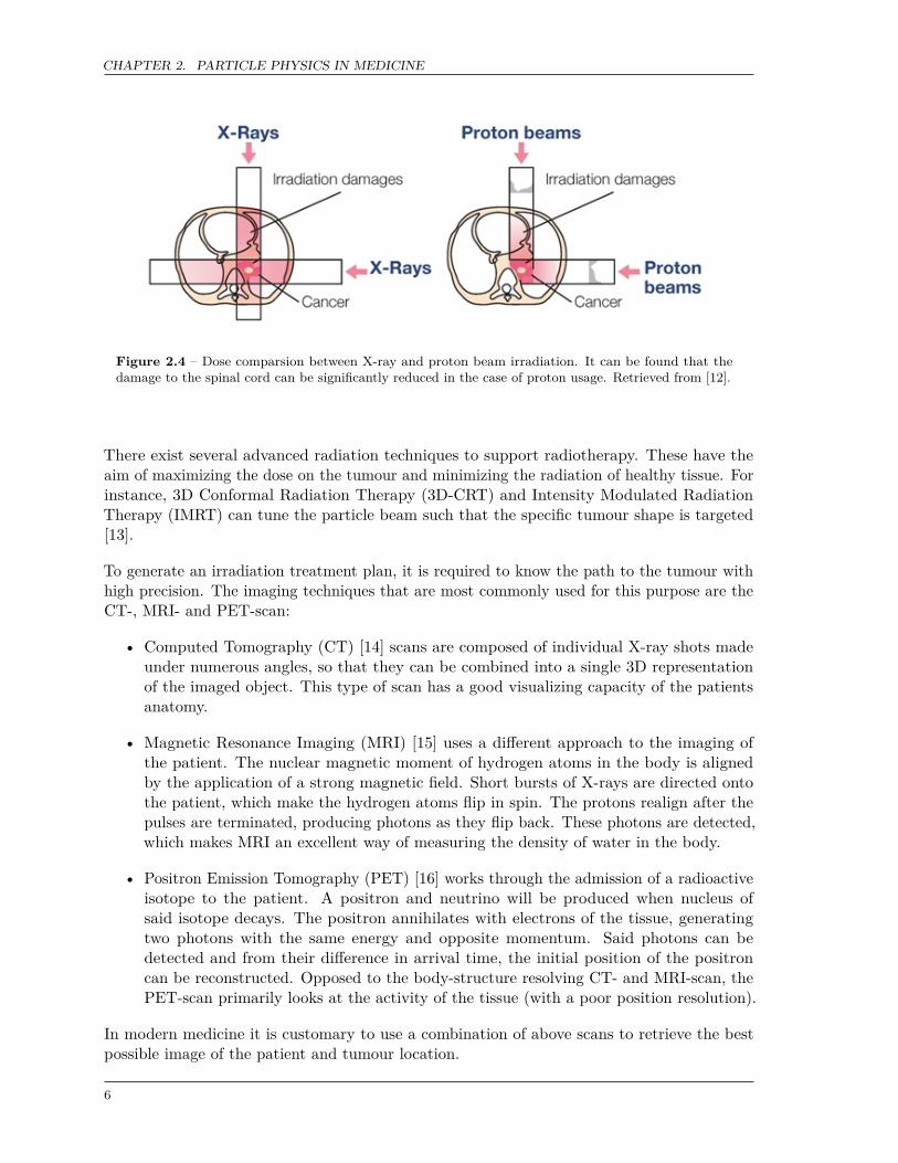
Figure 2.4 – Dose comparsion between X-ray and proton beam irradiation. It can be found that thedamage to the spinal cord can be significantly reduced in the case of proton usage. Retrieved from [12].
There exist several advanced radiation techniques to support radiotherapy. These have theaim of maximizing the dose on the tumour and minimizing the radiation of healthy tissue. Forinstance, 3D Conformal Radiation Therapy (3D-CRT) and Intensity Modulated RadiationTherapy (IMRT) can tune the particle beam such that the specific tumour shape is targeted[13].
To generate an irradiation treatment plan, it is required to know the path to the tumour withhigh precision. The imaging techniques that are most commonly used for this purpose are theCT-, MRI- and PET-scan:
• Computed Tomography (CT) [14] scans are composed of individual X-ray shots madeunder numerous angles, so that they can be combined into a single 3D representationof the imaged object. This type of scan has a good visualizing capacity of the patientsanatomy.
• Magnetic Resonance Imaging (MRI) [15] uses a different approach to the imaging ofthe patient. The nuclear magnetic moment of hydrogen atoms in the body is alignedby the application of a strong magnetic field. Short bursts of X-rays are directed ontothe patient, which make the hydrogen atoms flip in spin. The protons realign after thepulses are terminated, producing photons as they flip back. These photons are detected,which makes MRI an excellent way of measuring the density of water in the body.
• Positron Emission Tomography (PET) [16] works through the admission of a radioactiveisotope to the patient. A positron and neutrino will be produced when nucleus ofsaid isotope decays. The positron annihilates with electrons of the tissue, generatingtwo photons with the same energy and opposite momentum. Said photons can bedetected and from their difference in arrival time, the initial position of the positroncan be reconstructed. Opposed to the body-structure resolving CT- and MRI-scan, thePET-scan primarily looks at the activity of the tissue (with a poor position resolution).
In modern medicine it is customary to use a combination of above scans to retrieve the bestpossible image of the patient and tumour location.
6

CHAPTER 2. PARTICLE PHYSICS IN MEDICINE
2.3 Proton radiography
The Bragg peak of protons gives an excellent opportunity for cancer treatment. However, asthe path to the tumour is usually measured with a CT-scan (using photons), a calibrationbetween the interaction strength of protons and photons needs to be made.
The characteristic value of proton interaction - the proton stopping power (in MeV cm2 g−1) -is related (see Eq. 2.1) with absorbing material density via:⟨
−dEdx
⟩∝ Z
A(2.2)
In contrast, the photon interaction - the mass attenuation coefficient (in cm2 g−1) - is relatedby [17]:
µ ∝ Z
A
(KKN + Z1.86KSCA + Z3.62KPH
)(2.3)
with KKN the cross-section for free electrons, KSCA the cross-section for coherent scatteringand KPH the cross-section for the photoelectric effect.
A comparison between Eq. 2.2 and 2.3 shows that the underlying physical mechanisms of bothparticles are fundamentally different and a calibration will not be straightforward. Therefore,error margins are introduced on the location of the targeted material in the translation betweenboth. These margins reduce the benefit of proton therapy, as more healthy tissue will beradiated.
One method to solve this problem would be the usage of protons as imaging particles,introducing the field of proton radiography [18]. A proton beam with sufficient energy canpenetrate the body of the patient. As the particles’ energy loss in the soft tissue depends onthe type of material traversed, it is possible to construct a radiograph in this way.
In contrast to a CT-scan, where photons only scatter through the Coulomb force, the effect ofmultiple scattering of protons should be considered. The projection of the angular distributionfor the center 98% can be approximated as a Gaussian function, with the RMS given by [19]:
θ0 = 13.6MeVβcp
z√x/X0 [1 + 0.038 ln (x/X0)] (2.4)
with p the momentum, βc the velocity, z the charge number of the incident particle and x/X0the thickness of the scattering medium.
From Eq. 2.4 it can be found that highly energetic protons will exit the patient under asignificant angle (θ0 = 34 mrad for a 200 MeV proton in 10 cm of water). As the particles’energy loss depends on the traversed materials, this requires each proton to be trackedindividually. Using iterative software algorithms, the most likely path in the patient can beapproximated.
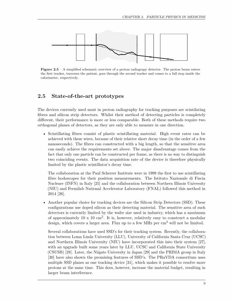
The requirement of measuring the particles’ scattering angle and energy loss lead to a distinctdetector design. The energy of the particles in the beam can be assumed to be constant, sothat the particles’ energy only needs to be measured after the patient. The general designused in proton radiography prototypes is shown in Fig. 2.5.
7
CHAPTER 2. PARTICLE PHYSICS IN MEDICINE
2.4 Challenges and aims
As proton therapy is being introduced in The Netherlands [20], the amount of effort put intoproton radiography is steadily increasing. This section lists the requirements necessary forproton radiography detectors, so that it will become clear where the current limitations lie andwhere more progress needs to be made. Before proton radiography devices can be commerciallyproduced and used in the hospital, attention to the following points must be given:
• It should initially be possible to construct radiograph of a typical organ, of which thedimensions are approximately 10 x 20 cm2. In some cases, it is possible to construct alarger area using multiple sub-detector as a larger detector. This will normally inducesome dead area in the image, which should be avoided as critical information can beeasily missed. It can additionally be taught of to combine several radiographs in orderto create a larger image. The disadvantage of this method is that a patient will move inbetween these measurements, reducing spatial resolution as a result.
• The spatial resolution is physically limited by the multiple Coulomb scattering in thepatient (see Eq. 2.4), which can be estimated to be in the order of 1 mm when advancedreconstruction algorithms are used [18]. This value is in the same order of magnitude ofthe margin in which a patient can be fixated during irradiation treatment [21]. A protonradiography detector should therefore be able to measure particles at this level.
• The density differences between types of soft tissues in the human body are in the orderof a percent [22]. As the proton source should be stable within 0.1% of its energy to allowfor proper accuracy [21], this thus will be not limiting for the detector. The differencesin density are directly related to stopping power (and thus residual energy), so a protonradiography detector should similarly be able to separate energies with a resolution lessthan 1%.
• As a patient has several movements during a radiograph (e.g. breathing, swallowing andheartbeat), the time that it takes to make a proton radiograph should be in the order ofa second. An image of 10 x 10 cm2 should be constructable with 106 proton tracks [23].A quick calculation learns that this requires the devices to run at a rate at least 1 MHz,assuming individual proton events. For eventual 3D reconstruction, a data acquisitionrate of ≥ 10 MHz is preferred [24].
• Proton radiography can be used as a quality control tool in proton therapy: a scan justbefore irradiation can provide the latest information on the tumour location. Resultsshould therefore be quickly available. A maximum processing time of around 15 minutescan be set, as this is approximately the time that it takes to remove the radiographydetector from the beam and everything is set up for irradiation.
There are other detector features that are not essential, but generally preferred. They includethe ability to track particles in 3D, in order to get more precise information on the angles ofthe proton tracks; it would be good if multiple particles can be measured at once, so that alarger read-out rate can be achieved; the detector should be as radiation hard as possible; andnot sensitive to temperature or humidity changes.
8
CHAPTER 2. PARTICLE PHYSICS IN MEDICINE
Figure 2.5 – A simplified schematic overview of a proton radiograpy detector. The proton beam entersthe first tracker, traverses the patient, goes through the second tracker and comes to a full stop inside thecalorimeter, respectively.
2.5 State-of-the-art prototypes
The devices currently used most in proton radiography for tracking purposes are scintilatingfibres and silicon strip detectors. Whilst their method of detecting particles is completelydifferent, their performance is more or less comparable. Both of these methods require twoorthogonal planes of detectors, as they are only able to measure in one direction.
• Scintillating fibres consist of plastic scintillating material. High event rates can beachieved with these wires, because of their relative short decay time (in the order of a fewnanoseconds). The fibres can constructed with a big length, so that the sensitive areacan easily achieve the requirements set above. The major disadvantage comes from thefact that only one particle can be constructed per frame, as there is no way to distinguishtwo coinciding events. The data acquisition rate of the device is therefore physicallylimited by the plastic scintillator’s decay time.
The collaboration at the Paul Scherrer Institute were in 1999 the first to use scintillatingfibre hodoscopes for their position measurements. The Istituto Nazionale di FisciaNucleare (INFN) in Italy [25] and the collaboration between Northern Illinois University(NIU) and Fermilab National Accelerator Laboratory (FNAL) followed this method in2014 [26].
• Another popular choice for tracking devices are the Silicon Strip Detectors (SSD). Theseconfigurations use doped silicon as their detecting material. The sensitive area of suchdetectors is currently limited by the wafer size used in industry, which has a maximumof approximately 10 x 10 cm2. It is, however, relatively easy to construct a modulardesign, which covers a larger area. Flux up to a few MHz per cm2 will not be limited.
Several collaborations have used SSD’s for their tracking system. Recently, the collabora-tion between Loma Linda University (LLU), University of California Santa Cruz (UCSC)and Northern Illinois University (NIU) have incorporated this into their system [27],with an upgrade built some years later by LLU, UCSC and California State University(CSUSB) [28]. Later, the Niigate University in Japan [29] and the PRIMA group in Italy[30] have also shown the promising features of SSD’s. The PRaVDA consortium usesmultiple SSD planes as one tracking device [31], which makes it possible to resolve moreprotons at the same time. This does, however, increase the material budget, resulting inlarger beam interference.
9

CHAPTER 2. PARTICLE PHYSICS IN MEDICINE
As for the measurement of the energy, two distinct ways to measure exist. One is themeasurement of a particle’s energy deposit inside detecting material, usually done usingcalorimeters; the other is to record how far a particle travels through the detecting materialuntil it comes to a full stop, as done by range telescopes. In some cases it is possible to combinethese signals, resulting in a hybrid detector.
• The kinetic energy of a particle can be recorded by getting it to a complete stop inside adetecting material and simultaneously measuring how much signal is generated. Themagnitude of this signal corresponds to particle’s kinetic energy, as shown by the Betheformula. These residual energy measurements are traditionally done with an organiccalorimeter, consisting of a crystal connected to a photomultiplier-tube. The maximumdata acquisition rate of these calorimeters is limited to a few tens of kHz, as their decaytime is rather long.
The LLU/UCSC/NIU collaboration has used CsI-crystals in their first design [27], theNiigate University uses a calorimeter of NaI [29] and the PRIMA-I collaboration used aYAG:Ce crystal [30], measuring at a rate of 10 kHz. The overall rate of these detectorscan be compensated using an array of segmented crystals, increasing the maximumreadout to 1 MHz in the PRIMA-II upgrade [32].
• A typical range telescope consists of multiple layers of sub-detectors, positioned behindone each other. When a particle traverses such a sub-detector, a signal will be generated.From the collection of signals it can be determined what the range of the incomingparticle in the detector was and the kinetic energy is reconstructed, as the relationbetween both is known to high precision.
Range telescopes can use a variety of materials, although plastic scintillators are the mostcommon because of their short decay time. Several collaborations, such as PSI (64 layersof 3mm) [33] and NIU/FNAL (96 layers of 3.2mm) [26], have used such scintillators intheir system. The INFN has used 60 layers of scintillating fibres [25] and the PRaVDAconsortium is testing the use of CMOS APS chips as a measurement device [31]. Thesechips are pixalated, which makes it possible to resolve multiple protons at the same time.All of these detectors have the capability of measuring at a rate of ≥ MHz, as requiredby proton radiography.
• A hybrid detector can measure the deposited energy of a particle in a detecting volume,without stopping it. By positioning several of these sub-detectors behind one eachother, the range of the particle can be measured in addition to its kinetic energy. Thesesignals are then combined, reducing the errors on the kinetic energy calculation. Hybriddetectors have not been used frequently up to now. Only the LLU/UCSC/CSUSBcollaboration has used a stack of five plastic scintillators in a full prototype for theirmeasurement [28].
From the collection of above designs it is clear that there is not much room for improvementin the current generation of prototypes, as multiple sub-detectors are necessary to achieve therequired performance. This work will investigate the operation of two new techniques in regardsto proton radiography, which are fundamentally different in operation: a Time ProjectionChamber for tracking purposes, which was developed in previous studies at Nikhef, Amsterdam;and hybrid silicon sensors for the combination of tracking and energy measurement.
10

CHAPTER 2. PARTICLE PHYSICS IN MEDICINE
The Time Projection Chamber investigated in this study has numerous benefits over othertracking devices. For instance, the TPC is able to track multiple particles at once, makingsure that the system is not initially limited in readout rate. Additionally, it is possible toperform 3D-reconstruction, from which more information on the incoming angle of the particlecan be retrieved than in the case of two points in tracking planes. Another major advantagecomes from the fact that the TPC is radiation hard, as there is a constant flow of ionizinggas. This makes sure that the detector will be stable over several years, necessary in aclinical environment. Most importantly, the interaction with the beam is significantly smallerin comparison with other detection methods. This will ultimately result in a better imageresolution.
The stack of hybrid silicon sensors is beneficial as they possess a high granularity. Similarto the TPC, this will allow for the processing of multiple particle as once, so that a higherparticle flux can be resolved. The combination of energy and range information should providea better energy resolution as two parameters are probed simultaneously. Additionally, theposition of entry on the chip can be used as a method of tracking. This makes a dedicatedtracker behind the patient redundant, which is beneficial in terms of detector cost and size.
11


3 | Detector overview
Previous chapter has motived the choice for a system based on a TPC as tracker and hybridsilicon sensor as deposited energy measurement device. This chapter will describe the individualcomponents of the two investigated prototypes - ProPix I and II - in more detail. Additionally,some attention will be given to the gas dynamics inside the TPC. To get an idea where theindividual components are located, the schematics of ProPix I and II are shown in Fig. 3.1and 3.2, respectively.
Figure 3.1 – ProPix I consists of a scintillator,two TPCs and a calorimeter. The scintillator isused as a timing reference when a proton entersthe detector. The two TPCs are used for track-ing purposes: one in front of the phantom, onebehind. The calorimeter consists of a BaF2 crystalconnected to a photo-multiplier tube.
Figure 3.2 – ProPix II consists of a TPC and twohybrid silicon sensors. As before, the TPC providesthe position measurement before the phantom.The silicon sensors simultaneously measure energyand position. A reference signal for the detector isnot required in this case, as this can be providedby one of the silicon sensors.
3.1 Time Projection Chamber
A Time Projection Chamber (TPC) (see Fig. 3.3) consists of a volume with a certain gas-mixture enclosed. When a charged particle travels through this chamber, ionisation of gasatoms can occur. The incoming particle loses a fraction of its kinetic energy, in turn liberatingan electron from the gas molecule. The probability in which this occurs depends on the atomselectron configuration and the energy of the incoming particle. The freed electrons are detectedindividually to allow track reconstruction.
First, a connection between a cathode at the top of the chamber and an anode at the bottomis made. The cathode is put at a relatively high voltage (in the order of several hundreds ofV/cm), so that its electric field drifts the created electrons downwards. A high drift velocity isbeneficial in terms of data-acquisition rate, a low drift velocity in terms of z-resolution.
13

CHAPTER 3. DETECTOR OVERVIEW
Figure 3.3 – A schematic overview of the processes occurring in the Time Projection Chamber, with a 1kV/cm drift field, 1280 V GEM voltage and 2 kV/cm transfer field. A particle enters from the left andionizes the gas. The freed electrons drift downwards by the electric field applied by the cathode on top.The electric field is kept homogeneous by the copper strips, decreasing in voltage every step. An electroncloud is generated by the passage of the several GEMs. Finally, the signal is collected at the chip.
Assuming that the electric field is properly configured, the x/y-position at arrival at the anodeplane should be representable of the initial electron position. The z-direction can be calculatedby measuring the time for which it takes the electron to move downwards, as the drift velocityin the gas is known. This measurement requires a reference time, which can be provided bye.g. a scintillator in the plane of the particle. From the collection of measured electrons, atrack can be constructed. More specifically, the incoming position of the particle with itscorresponding entry angles can be found.
To make sure that the correct origin of the created electrons is retrieved, the electric fieldneeds to be as homogeneous as possible. This is assured by a field cage enclosing the TPC, sothat the largest distortions in the field are cancelled. The field cage consists of a 50 µm thickcapton foil, with 0.5 mm of copper strips every mm. These strips are connected by a chain of10 MΩ resistors, dividing the voltage linearly over the active volume.
The electrons diffuse in both longitudinal and transverse direction due to interactions withthe gas. The diffusion is thus dependant on the mixture of the gas and on the voltage of thecathode; both need to be carefully tuned as a low diffusion is required for a proper functioningtracker. As the diffusion can be expected to be of Gaussian shape, the mean deviation in boththe x/y as the y/z-plane can be written as [34]:
σi = Di
√L (3.1)
with L the traversed distance and Di the diffusion coefficient.
14

CHAPTER 3. DETECTOR OVERVIEW
Figure 3.4 – The geometry of a single GEM foil.Holes of 70 µm in diameter are drilled every 140 µm.Secondary electrons are generated in the holes inthe copper-capton-copper foil. Drawing adaptedfrom [35].
Figure 3.5 – An electron avalanche is createdafter a single incoming electron passes a stack ofthree GEM foils. The voltages are tuned througha resistor circuit. Drawing adapted from [36].
3.2 Gas Electron Multiplier
Only a few tens of electrons are generated per passing particle in the TPC. These electrons donot induce enough current in a measurement device to create a signal. The current thereforeneeds to be strengthened in some way: Gas Electron Multiplier (GEM) foils [37], produced atCERN, Geneva, are used for this purpose. These foils can be put over a bare chip, withoutany need for post-processing.
The schematic of a GEM foil is shown in Fig. 3.4. The GEM used in this study is made of50 µm capton foil, with a 5 µm copper foil enclosing it on both sides. Holes with an innerdiameter of 50 µm and an outer diameter of 70 µm are drilled in the foil every 140 µm over theentire surface. The canonical shape of the holes is therefore due to the manufacturing process.Even rows have an offset in relation to the odd rows, so that more area is covered.
A relatively high voltage of ≈ 8-10 kV/mm is applied between the copper layers. These layersact as a parallel plate capacitor, as they are not physically connected. When an electron passesthrough a hole, the gas will be ionized further so that secondary electrons are produced. Thenumber of electrons produced (or gain) depends on the strength of the electric field. TheTownsend coefficient can be used to classify the gain: if a value ≥ 1 is achieved, multiplicationwill occur. A high electric field increases the probability of discharges, so the involved voltagesshould be carefully tuned.
To achieve a higher gain, it is possible to stack multiple GEM foils, as is shown in Fig. 3.5. Thesecondary electrons from the first foil will drift towards the second GEM foil, where anothermultiplication step occurs. Finally, when the third GEM foil is passed, the signal is amplifiedso much (up to a million electrons) that the induced charge can be detected in the readoutunit.
A dedicated control system has been designed to tune the voltage on each GEM. Thisadditionally makes sure that the best values for the transfer field can be chosen, so thatdiffusion is reduced to a minimum. The volume between the lowest field cage strip and theupper GEM foil must be carefully monitored, as both are supplied by a different high-voltagegenerator.
15

CHAPTER 3. DETECTOR OVERVIEW
Figure 3.6 – The timing inside of the Timepix3.The TOT is determined from the number of timesthat the internal 40 MHz clock is above thresholdlevel. The TOA is determined by the combinationof the internal 40 MHz clock and the fast 640 MHzcounter that starts running when the threshold issurpassed. Drawing adapted from [4].
Figure 3.7 – The effect of timewalk in theTimepix3. A highly-energetic particle will buildup charge faster in the pixel than a lower-energeticone, which leads to a different Time Of Arrival forboth particles. Drawing adapted from [38].
3.3 Timepix3 readout chip
The Timepix3 [40] stems from the Medipix family, which has been developed at CERN, Genevain collaboration with Nikhef, Amsterdam. The chip has 256 x 256 pixels with a size of 55 x55 µm each. It is based on 130 nm CMOS technology and can be classified as a hybrid pixeldetector.
When the collected charge passes a threshold, which can be set for every pixel individually,a 640 MHz clock will start to run until a reference point of the 40 MHz internal clock isreached. The Time Of Arrival (TOA) is determined by the combination of these two clocks.Additionally, the Time Over Threshold (TOT) is recorded as a measurement of the totalcollected charge. For a summary of this process, see Fig. 3.6.
The chip can be read out in tree distinct readout modes: collecting TOA and TOT (done inthis work), collecting only TOA, or collecting only the number of counts. The read-out can beeither frame based or data driven and there exists a zero suppressed readout. The inducedcurrent on the chip has a limited rise time. For large deposits, the rise is faster than for lowones (see Fig. 3.7). As the threshold is a fixed value, the Time Of Arrival will be differentfor the particles. This effect is called timewalk. The relation between TOT and TOA can bemeasured in order to quantify this effect and make corrections.
A dedicated chip-board for the Timepix3 chips has been designed. Both quad-boards (in a2x2 array of chips) and single-boards are available. The readout is performed by the SPIDRunit [41], which is able to send data at a frequency of 80 MHz per chip. A reference clock andindependent trigger can be used as input for the SPIDR.
Instead of gas, it is possible to connect a silicon sensor to the Timepix3. These detectors willbe referred to as hybrid pixel sensors. The configuration of a single pixel is drawn in Fig.3.8. When a charged particle traverses the silicon layer, many electron-hole pairs are created.Depending on the applied bias voltage, either holes or electrons drift towards the implants. Asufficient current is generated without any need for further amplification, in contrast to theTPC.
16

CHAPTER 3. DETECTOR OVERVIEW
Figure 3.8 – Schematic overview of the combin-ation of a silicon active layer, bump-bonded ontothe Timepix3 ASIC. Retrieved from [39].
Figure 3.9 – Schematic overview of the triggerlogic in ProPix I. Based on information from [4].
3.4 Calorimeter and trigger
The calorimeter used in ProPix I consists of a BaF2 crystal [42] combined with a photomultiplier-tube. Electrons in the crystal get exited when a charged particle enters, releasing photons asthey fall back to their ground state. The total number of photons created is proportional tothe initial kinetic energy of the incoming particle.
The scintillation light of the BaF2 crystal consists of two components: one with a decay timeof 600 ps, used for trigger purposes, and the other of 630 ns, used for the measurement of theenergy. The digitization of these analogue signals is done with a CAEN Digitizer [43]. Theentire configuration can measure at a data-acquisition rate of approximately 10 kHz.
A trigger configuration has been made in order to synchronize the multiple sub-systems inProPix I, which can be found in Fig. 3.9. The signals from both scintillator and calorimeterpass through a discriminator in order to create a digital signal. When both coincidence, atimer is started. This timer shuts the data-acquisition system for the time that it takes allgenerated electrons in the TPC to drift downwards, approximately 100 µs. Afterwards, theread-out timer is started to make sure the data-acquisition system is not overloaded withevents. When all data is written, it is reset.
17


4 | ProPix I prototype
This work continues upon the results achieved by [4], in which a set-up as is shown in Fig. 3.1has been used. A careful examination of former achieved test beam data - collected at KVI,Groningen [44] in 2015 - is made in this chapter. It will be shown that several irregularitiesare present in the data, for which, wherever possible, solutions are proposed. A complete dataanalysis is presented afterwards.
4.1 Large clustersize
One of the found deviations relates to the size of the measured signals. It is observed thatclusters of up to ten pixels in width appear in the tracks, as can be seen in a typical protonevent in Fig. 4.1. This effect would result a limited spatial resolution, as the clustersize is notconstant and edge effects occur; and a lower data acquisition rate, as the information for morepixels needs to be transmitted.
Figure 4.1 – A typical proton event registered in the TPC in front of the phantom.
The large signal size could arise from the diffusion of the electrons in the gas, as a higherdiffusion results in more spread of charge. To quantify this effect, a simulation in Garfield++[45] and Magboltz [46] of several gasses is made. The selection of gasses chosen for thesimulation is made based on the availability and frequency of usage in detector experiments[47]:
DME:CO2 (50:50) Ar:CF4:CO2 (45:40:15)Ar:CO2 (90:10) Ar:CF4:iC4H10 (95:3:2)He:iC4H10 (80:20) Ar:iC4H10 (90:10)He:CO2 (90:10) Ar:CF4:CH4 (75:20:5)
19

CHAPTER 4. PROPIX I PROTOTYPE
Figure 4.2 – A schematic overview of the diffusionof charge between the GEMs and the chip. In dark-red, the behaviour that is desired. In light-red, thebehaviour that is most probably due to diffusionof the electrons.
Figure 4.3 – The simulated gas flow inside theTPC. The background color is a measure of theabsolute velocity at this point, the arrows representthe direction of the flow. A counter-clockwise flowis observed in the drift volume.
The drift velocity, transversal and longitudinal diffusion are calculated and shown in Fig.4.3a, 4.3b and 4.3c, respectively. During the proton test beam, the gas-mixture Ar:CF4:CO2(45:40:15) was used at a transfer voltage of 3 kV/cm. This mixture was chosen because of therecommendation of the GEMPIX-collaboration [48]. From the simulation it can be found thata transversal drift is DT ≈ 100 µm/
√cm is found in this case.
Previously, the relation between the diffusion coefficient and the mean displacement was given(Eq. 3.1). For the distance between the second and third GEM (L = 2 mm), this gives: σT
= 44.7 µm. As the distance between two holes in the GEM is only 70 µm, it is evident thatelectrons can travel to other holes after a width of only ≈ 1.5σ. The resulting avalanches willtherefore spread the charge over multiple pixels (see Fig. 4.2). This behaviour is confirmed bysimulation studies [49].
The only simulated gas that has a lower diffusion than the previous mentioned gas, is theDME:CO2 (50:50) mixture. This gas needs to be operated at a higher cathode electric field inorder to retrieve the same gain. As the difference in diffusion over a few millimetre is veryminimal, it is however not expected that the clustersize would be significantly improved by achange of gas.
When the entire drift distance of the chamber is considered (500 mm) however, an improvementcan be made. It is proposed to use a 1 kV/cm field with DME:CO2 (50:50), instead of the300 V/cm field with Ar:CF4:CO2 (45:40:15) in order to reduce the amount of cluster diffusion.The results of this change will be discussed later.
Concluding, this study shows that it is possible for diffusion to be the origin of the large signalsize. A change of gas would not resolve this problem. One other possibility is that the gain ofthe GEM foils is set too high, so that more electrons are produced than necessary for detection.It will be later investigated which settings of the voltages on the GEM foils result in the bestperformance.
20

CHAPTER 4. PROPIX I PROTOTYPE
a – Drift velocity.
b – Transverse diffusion.
c – Longitudinal diffusion.
Figure 4.4 – Simulated properties of a selection of gasses. Marked are 300 V/cm (the used drift field value inProPix I) and 1000 V/cm (the proposed drift field value for ProPix II).
21

CHAPTER 4. PROPIX I PROTOTYPE
a – Row hit-distribution. b – Column hit-distribution.
Figure 4.5 – The hit distributions for both the column as the row for the TPC behind the phantom.
4.2 Gas flow in chamber
Data analysis reveals that the distribution of hits is not uniformly spread over the area of thechip, as can be seen in the column- and row distributions in Fig. 4.5. More hits are presenttowards the edges of the chamber. The flow of ionising gas inside the TPC could influence theprocesses that occur inside the TPC, as the gas density is related with the number of detectedelectrons by the amount of electron capture and number of primary ionizations.
To study the flow rate inside the chamber, the active gas volume is modelled and a two-dimensional fluid flow simulation is made in OpenFOAM [50]. The results are visualised withthe ParaFOAM plug-in, which is based on ParaView [51]. As the changes in temperature andpressure are expected to be small over time, the gas will be modelled as an incompressiblelaminar fluid. A flow of gas is launched with an arbitrary velocity from the inlet at the bottomof the chamber, and collected from the outlet on the top. For simplicity, the GEM foilsare simulated as being an open volume in which the gas can freely travel. Additionally, thediffusion from the sides of the chamber is neglected, as there is no proper way to quantify thiseffect. Iterations are performed up until a steady-state solution is found.
The results of above simulation are shown in Fig. 4.3. The arrows represent the direction ofthe flow, with their size and the background colour visualising the magnitude. It becomesclear that a relative anti-clockwise flow exists in the chamber, with the majority of the streambeing collected at the outlet.
One interesting aspect comes from the lack of flow in the center of the TPC. If air from outsideis trapped inside this area, less ionised electrons will reach the bottom due to electron capture.This means that there will be a relative stronger signal towards the edges of the collectingchips. This behaviour is in agreement with the hit distributions as found in Fig. 4.5.
It is, however, unlikely that the gas flow can have such major impact on the hit-distribution, asprocesses such as turbulence will eventually distort the steady state. Other explanations havebeen found for the unusual shape of the signal in the hit-distribution, which will be discussedbelow. Still, the relation between the shape of the signal and the elapsed time will be studiedlater to make sure no unwanted effects arise.
22

CHAPTER 4. PROPIX I PROTOTYPE
a – The TPC in front of the phantom. b – The TPC behind the phantom.
Figure 4.6 – Protons are entering the TPC from the top, for which only tracks of specific entry regionsare drawn. This results in the average path the protons travelled in the TPC, which gives a good indicationon the positions where curvature occurs.
4.3 Electric field distortions
Tracks in the chambers are found to posses a non-negligible curvature in both the x/y as thez/y-plane. These electric field distortions would result in a reduced spatial resolution, as theposition information from the tracks is less precise. Both large scale (evident in Fig. 4.6), assmaller scale (in the order of a few pixels) effects are present. Explanations for the severalphenomena are presented below.
S-like curvature x/y-plane
In the TPC behind the phantom (Fig. 4.6b) the tracks are found to have a S-like shape. Similarbehaviour is found in the TPC in front of the phantom, but in this case to a lesser extent. Itis likely that these problems arise due to a discrepancy in the homogeneity of the electric fieldinside the chamber.
As was stated before, the hit-distributions (Fig. 4.5) show an increase in the number of hitstowards the edges of the chamber. The hit-distribution of the column shows other effects aswell, which will be discussed later. The increase of the numbers of hits towards the edgescould indicate that an electric field is present in all edges, pointing towards the center of thechamber.
One possible explanation for these effects comes from the existence of a strip of insulatingmaterial inside the chamber. It could be that this strip charges up during the measurements,as the electrons have no way to escape the material. This electric field will drift the electronstowards the center of the chamber: exactly what is found in the distribution of hits. Anotheroption would be that the voltage on the field cage is not properly configured. If this voltage isset too high, electrons could similarly drift from the side of the chamber inwards.
23
CHAPTER 4. PROPIX I PROTOTYPE
a – Potential map. b – Drift lines.
Figure 4.7 – The simulated properties of the electric field in the case of an incorrectly set potential onthe field cage. Electrons curve from the edges of the TPC inwards.
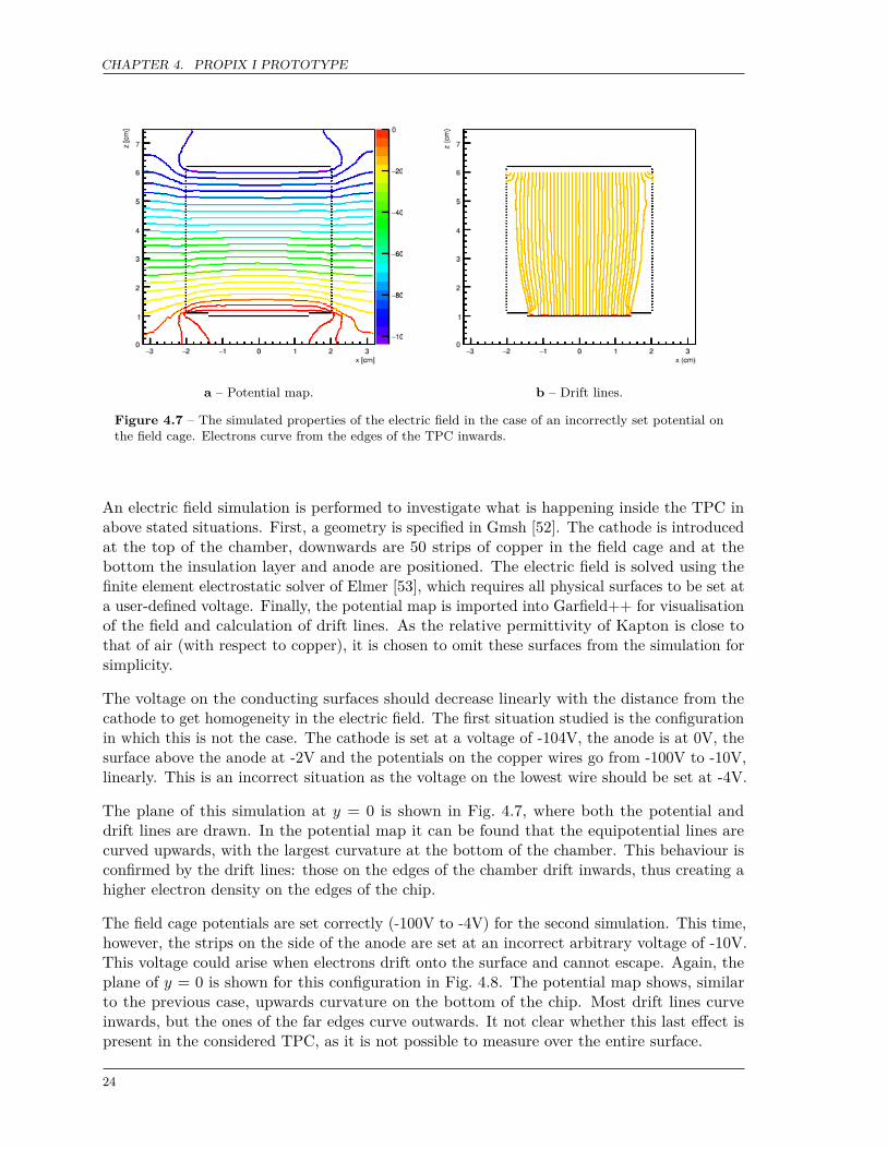
An electric field simulation is performed to investigate what is happening inside the TPC inabove stated situations. First, a geometry is specified in Gmsh [52]. The cathode is introducedat the top of the chamber, downwards are 50 strips of copper in the field cage and at thebottom the insulation layer and anode are positioned. The electric field is solved using thefinite element electrostatic solver of Elmer [53], which requires all physical surfaces to be set ata user-defined voltage. Finally, the potential map is imported into Garfield++ for visualisationof the field and calculation of drift lines. As the relative permittivity of Kapton is close tothat of air (with respect to copper), it is chosen to omit these surfaces from the simulation forsimplicity.
The voltage on the conducting surfaces should decrease linearly with the distance from thecathode to get homogeneity in the electric field. The first situation studied is the configurationin which this is not the case. The cathode is set at a voltage of -104V, the anode is at 0V, thesurface above the anode at -2V and the potentials on the copper wires go from -100V to -10V,linearly. This is an incorrect situation as the voltage on the lowest wire should be set at -4V.
The plane of this simulation at y = 0 is shown in Fig. 4.7, where both the potential anddrift lines are drawn. In the potential map it can be found that the equipotential lines arecurved upwards, with the largest curvature at the bottom of the chamber. This behaviour isconfirmed by the drift lines: those on the edges of the chamber drift inwards, thus creating ahigher electron density on the edges of the chip.
The field cage potentials are set correctly (-100V to -4V) for the second simulation. This time,however, the strips on the side of the anode are set at an incorrect arbitrary voltage of -10V.This voltage could arise when electrons drift onto the surface and cannot escape. Again, theplane of y = 0 is shown for this configuration in Fig. 4.8. The potential map shows, similarto the previous case, upwards curvature on the bottom of the chip. Most drift lines curveinwards, but the ones of the far edges curve outwards. It not clear whether this last effect ispresent in the considered TPC, as it is not possible to measure over the entire surface.
24

CHAPTER 4. PROPIX I PROTOTYPE
a – Potential map. b – Drift lines.
Figure 4.8 – The simulated properties of the electric field in the case of an charging insulating surface.Most electrons move from the edges of the TPC inwards, but a significant fraction curves towards thefield cage.
If there exists a relative electric field pointing towards the center of the chamber, the electronsgenerated by the proton track drift towards the center. As the proton enters the TPC under asmall angle, the S-shape in the x/y-plane is explained. This process is visualised schematicallyin Fig. 4.9.
To conclude, the major S-shaped curvature in the x/y-plane of the TPC is most likely due toa combination of insulating material in the field cage and not correctly set field cage voltages.The first effect can be resolved when a proper ground around the GEM foils is introduced.The second by careful tuning of the voltages involved in the field cage.
Focal point x/y-plane
In the chamber in front of the TPC (Fig. 4.6b) the tracks in the bottom-left of the chamberdeviate towards a focal point. If the geometry of the chamber is compared with the positionof this focal point, it is concluded that it is most likely that this effect is caused by the highvoltage supply towards the GEM. This supply cable is not properly shielded, which makes itpossible for electrons to drift towards this copper strip for them to be collected. This problemcan be easily resolved when some electrical tape is placed over the affected cable.
U-like curvature z/y-plane
The tracks of the protons show an U-like shaped distortion in the z/y-plane. This meansthat the reconstructed tracks curve slightly upwards towards the edges of the board. Thiseffect occurs when the Time Over Threshold value is not properly defined for the edges of thechips. It can happen that only a fraction of a signal is detected, so that the average TOT issignificantly lower than in the center of the chip. As the timewalk-correction relates the valuesof the TOT with the TOA, this will result in incorrect TOA values.
25

CHAPTER 4. PROPIX I PROTOTYPE
Figure 4.9 – Explanation of the S-like curvature x/y-plane. As the proton enters the TPC, electronsare generated over the entire surface. However, as there is a relative electric field pointing inwards, theelectrons towards the edges of the chamber are pushed inwards, resulting in the S-shaped track.
This effect would be hard to get rid of physically, as ideally the clustersize should be reduced.The best way to deal with it is to define an active area of the chip that is slightly smaller thanthe physical size. As the clusters have been observed to be up to ten pixels in width, this willbe a starting point for the decrease in active chip area from the edges.
Small deviations z/y-plane
Additionally to the U-shaped distortion in the z/y-plane, smaller deviations of the tracks overthe region of the chips are found. Again, this is a problem related to the timewalk-correction.The first generation of Timepix3 chips had a defect, which caused the threshold level not tobe constant over the entire surface of the chip [38]. More specifically, it was found that thereis a dependence on the column number. This results in a deviation in TOT values, and thus,by the timewalk correction, in TOA deviations as a function of chip column.
The newest generation of Timepix3 chips have had this defect in the chip-design resolved, butthese chips are unavailable for this research. It is therefore not possible to resolve this effectphysically. An adjustment in the data-processing software will have to be made, in order tocorrect for this effect.
Small deviations x/y-plane
Similar to the deviations in the z/y-plane, deviations of small size are found in the x/y-plane.As the average threshold is not constant over the columns (due to the error in chip design),the resulting number of hits will be different as well. This behaviour can be found in thedistribution of hits as a function of column number (Fig. 4.5) as two large maxima in additionto the bias towards the edges. If some regions produce more hits than others, the fittedtrack will be biased towards the high hit-density region. This effect is then observed as smalldeviations close to the high hit-density regions.
Above effect will be resolved in the analysis by grouping neighbouring hits together in clusterswith a single center of gravity point. As not all individual hits are used in this case, theresponse of the chip will be equal over the entire surface and the discussed effect shoulddisappear.
26
CHAPTER 4. PROPIX I PROTOTYPE
a – Raw hits. b – Clustered hits. c – Center of gravity.
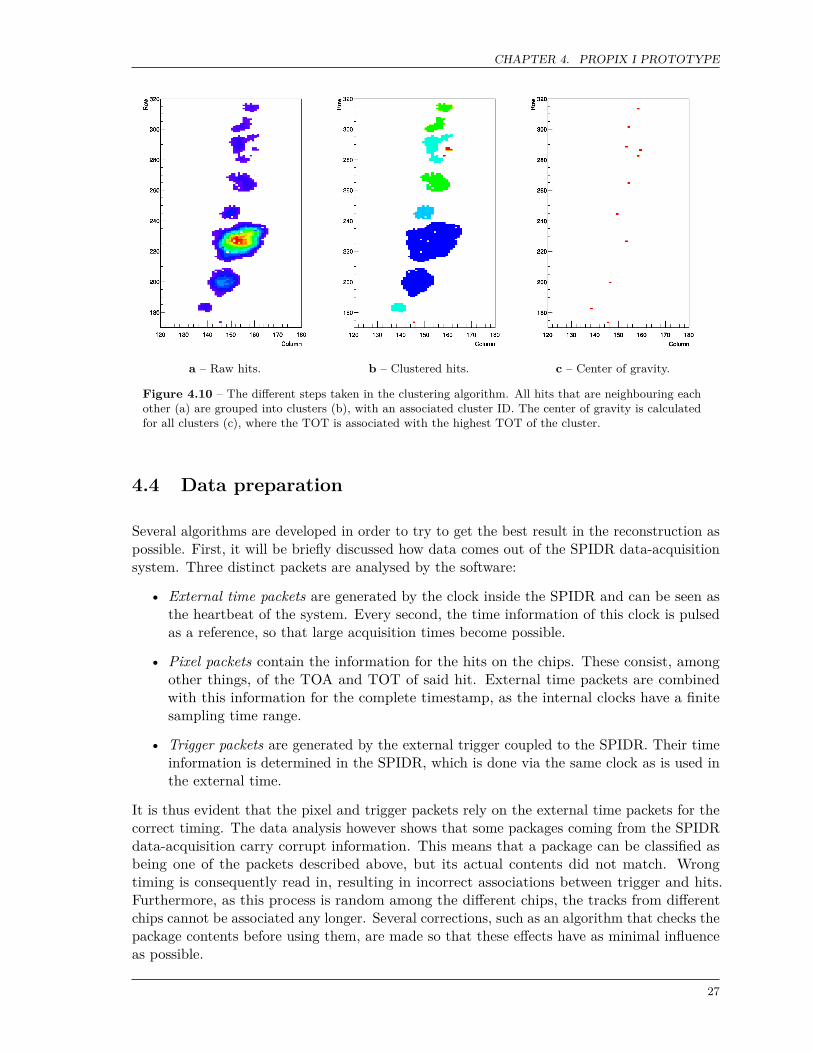
Figure 4.10 – The different steps taken in the clustering algorithm. All hits that are neighbouring eachother (a) are grouped into clusters (b), with an associated cluster ID. The center of gravity is calculatedfor all clusters (c), where the TOT is associated with the highest TOT of the cluster.
4.4 Data preparation
Several algorithms are developed in order to try to get the best result in the reconstruction aspossible. First, it will be briefly discussed how data comes out of the SPIDR data-acquisitionsystem. Three distinct packets are analysed by the software:
• External time packets are generated by the clock inside the SPIDR and can be seen asthe heartbeat of the system. Every second, the time information of this clock is pulsedas a reference, so that large acquisition times become possible.
• Pixel packets contain the information for the hits on the chips. These consist, amongother things, of the TOA and TOT of said hit. External time packets are combinedwith this information for the complete timestamp, as the internal clocks have a finitesampling time range.
• Trigger packets are generated by the external trigger coupled to the SPIDR. Their timeinformation is determined in the SPIDR, which is done via the same clock as is used inthe external time.
It is thus evident that the pixel and trigger packets rely on the external time packets for thecorrect timing. The data analysis however shows that some packages coming from the SPIDRdata-acquisition carry corrupt information. This means that a package can be classified asbeing one of the packets described above, but its actual contents did not match. Wrongtiming is consequently read in, resulting in incorrect associations between trigger and hits.Furthermore, as this process is random among the different chips, the tracks from differentchips cannot be associated any longer. Several corrections, such as an algorithm that checks thepackage contents before using them, are made so that these effects have as minimal influenceas possible.
27

CHAPTER 4. PROPIX I PROTOTYPE
a – Tracks as they are recorded. b – Tracks after the procedure.
Figure 4.11 – Overview of the straighting procedure on the tracks in the TPC before the phantom. Notethat the tracks on the edges start to approach each other.
One of the chips in the chamber before the phantom had incorrect settings applied to it, as itsthreshold-level was set too low. Concretely, this means that the chip had many more firingpixels compared the other chips in the configuration. Corrections are implemented in theentire software package, so that relative differences are used in the timing information insteadof absolute ones. The most probable track is furthermore selected using the height of the TOTvalues, resulting in an improved signal-to-noise ratio and more usable data for this specificchip.
The offset between trigger information and pixel hits is not of constant value, as the chips onthe quad-board were not reset simultaneously during the test beam. This offset is randomfor every run and involved chip. When multiple runs are combined, this would result inan undesired offset in the z-direction of the tracks and hence this should be resolved. It ischosen to make the evaluation of the integral over the correlations between pixel and triggerinformation. The retrieved offset is the mean of the found distribution, which gives a stableresults for all runs.
As was noted before, the number of pixels hit by an electron in the TPC has a major fluctuation.It is not expected that the observed width of these clusters is correlated with the physicalprocesses occurring inside the chamber, so it is decided to develop a clustering algorithm. Thiswill make sure that all data-points are treated with the same weight and hence some of theeffects described on the electric field distortions should disappear.
A simple next-neighbour design is constructed (see Fig. 4.10): all hits that are neighbouringeach other are grouped into clusters. This procedure fails when clusters are overlapping eachother, since they will be recognised as one. It is however expected that the improvement isgreater than the errors induced. As the deviations in shape, TOT values and size are toolarge to introduce pattern recognition, it is unlikely that more complex models will have anincreased positive influence on the obtained results.
28

CHAPTER 4. PROPIX I PROTOTYPE
a – The complete phantom. b – The measured area of the phantom.
Figure 4.12 – Overview of the irradiated phantom, with the measured region marked. See the text forthe material compositions. Based on information from [5].
To correct for the curvature effects, an offset algorithm is created. For every hit, the normalizeddifference between its position and the average column number is calculated in both the x/y-and x/z-plane. This offset is subtracted from the hits, so that a more straight field is found.No fitting algorithm is applied in this step as the shape of the distortions has previously beenfound to consist of several effects. The result of this procedure is found in Fig. 4.11.
Note that only curvature is adjusted in the offset procedure, not the uniformity. Unfortunately,a correction for the uniformity is not possible to be made, as the distribution of hits on thecolumns is under influence of the threshold (Fig. 4.5b). These effects are most significant onthe edges of the chamber, making it possible to have shaping effects on the borders of theradiograph. These edges are not analysed for this reason.
A number of cuts are performed on the found tracks in order to improve the signal-to-noiseratio. All hits on the far edges of the chips are first removed, as they do not carry reliabledata due to the width of the clusters. Hits with fewer than 5 TOT-counts are ignored, as theycan be expected to be noise. The tracks inside the chambers are fitted with linear functionsin both the x/y- as the x/z-plane. The reduced χ2 is tracked in order to exclude odd events(delta rays, etc.) from the data. Using the information of both chambers, the most likely pathof the proton is approximated using a simple track-fitting algorithm.
Several other additions are made to retrieve the best data quality. It is made sure that data isnot multiply assigned over events, so that no non-physical connections are made. An offsetcorrection for the different SPIDR times is made, which is due to incorrect values in the triggerpackets. New is the association between the chamber before and after the TPC, so that aninvestigation of multiple scattering becomes possible for the first time. Finally, all differentprocesses are grouped in one single analysis tool, aiding the speed of the system as well as theease of its sustain.
29
CHAPTER 4. PROPIX I PROTOTYPE
a – Deposited energy (arb. units). b – Multiple scattering magnitude (arb. units).
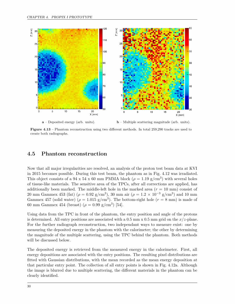
Figure 4.13 – Phantom reconstruction using two different methods. In total 259,290 tracks are used tocreate both radiographs.
4.5 Phantom reconstruction
Now that all major irregularities are resolved, an analysis of the proton test beam data at KVIin 2015 becomes possible. During this test beam, the phantom as in Fig. 4.12 was irradiated.This object consists of a 94 x 54 x 60 mm PMMA block (ρ = 1.19 g/cm3) with several holesof tissue-like materials. The sensitive area of the TPCs, after all corrections are applied, hasadditionally been marked. The middle-left hole in the marked area (r = 10 mm) consist of20 mm Gammex 453 (fat) (ρ = 0.92 g/cm3), 30 mm air (ρ = 1.2 × 10⁻³ g/cm3) and 10 mmGammex 457 (solid water) (ρ = 1.015 g/cm3). The bottom-right hole (r = 8 mm) is made of60 mm Gammex 454 (breast) (ρ = 0.99 g/cm3) [54].
Using data from the TPC in front of the phantom, the entry position and angle of the protonsis determined. All entry positions are associated with a 0.5 mm x 0.5 mm grid on the x/z-plane.For the further radiograph reconstruction, two independant ways to measure exist: one bymeasuring the deposited energy in the phantom with the calorimeter; the other by determiningthe magnitude of the multiple scattering, using the TPC behind the phantom. Both methodswill be discussed below.
The deposited energy is retrieved from the measured energy in the calorimeter. First, allenergy depositions are associated with the entry positions. The resulting pixel distributions arefitted with Gaussian distributions, with the mean recorded as the mean energy deposition atthat particular entry point. The collection of all entry points is shown in Fig. 4.12a. Althoughthe image is blurred due to multiple scattering, the different materials in the phantom can beclearly identified.
30

CHAPTER 4. PROPIX I PROTOTYPE
z (mm)0 2 4 6 8 10 12 14 16 18 20 22
Sca
led
valu
e (a
rb. u
nits
)
2−
1−
0
1
2 Energy deposition
Multiple scattering
Figure 4.14 – Section at z = 18 mm in a grid of 1 mm x 1 mm for both the energy deposition and themultiple scattering.
Similarly, a radiograph can be made by investigation of the multiple scattering magnitude. Theposition of the first TPC is again used as entry point, but now the information of the secondTPC is used instead of the calorimeter. The difference in entry and exit position is recordedfor all tracks. It is expected that the resulting distributions on every entry point follow aGaussian distribution (see Eq. 2.4). The width of said distribution is used as a measurementof the multiple scattering. A radiograph of this sort is shown in Fig. 4.12b.
Whilst the same pattern is present is this case, there is more noise. The first reason for thisbehaviour comes from the fact that more data is required to get a proper estimate of thewidth of the distribution than in the case of a measurement of the mean. More recorded trackswould solve this issue. The second reason is due to the fact that particles scatter away fromthe second TPC, which means only part of the distribution is found towards the edges. Thiscomplication could be resolved if either the TPC behind the phantom is increased in activearea, or placed closer to the phantom.
To show the transition between the different materials, the section at z = 18 mm is taken fora grid size of 1 mm x 1 mm (values as desired for clinical application) and scaled for both thedeposited energy and the multiple scattering. This slice can be found in Fig. 4.14, in whichthe errors bars are found from the errors on the fitted parameters of the distributions. Thetransition between the two materials is clear in the case of the energy deposition; for multiplescattering there is more variation.
The difference in energy deposition between the two materials is (in arbitrary units):
∆E = (1.00± 0.04)− (−1.00± 0.08) = 2.00± 0.09 (4.1)
The density resolution of the detector can be determined from this information, as the differencein density of the irradiated materials is known and (from Eq. 2.2) it is known that the energydeposition scales linearly with the density of the material. The density difference is given by:
∆ρ = 1.19−(0.92× 20mm + 1.02× 10mm
60mm
)= 0.71 g/cm3 (4.2)
31

CHAPTER 4. PROPIX I PROTOTYPE
Figure 4.15 – The correlation between deposited energy and multiple scattering.
Therefore, as it can be assumed that the uncertainty between the two measured points scaleslinearly and signals can be distinguished at a 1σ-level, the density resolution becomes:
ρres = ∆ρ× σE
∆E = 0.71× 0.092.00 = 0.03 g/cm3 ≈ 2.5% (4.3)
One way to distinguish the different materials is to make a correlation plot between the energydeposition and the multiple scattering. This correlation is shown in Fig. 4.15. Although theimage is heavily blurred due to multiple scattering, two ellipses for the different materials canbe found. As the scattering radiograph provides information on the radiotion length of thetraversed materials (see Eq. 2.4) and the deposited-energy radiograph gives information onthe density of the traversed materials (see Eq. 2.1), the combination made in Fig. 4.15 can bea powerful tool of separating different materials and deserves further investigation in futurework.
32

5 | ProPix II prototype
Through simulations it is investigated how the proposed detector layout (see Fig. 3.2) wouldperform as a proton radiography device. The interference of the trackers on the proton beam isdetermined; the study of a typical phantom is made; and the best way to measure a particle’senergy is determined. All studied simulation configurations can be found in Fig. 5.1, as areference point. Following this, the various optimisations on the hardware of ProPix II areshown using a radioactive source.
5.1 Prototype simulations
The software-framework of Geant4 [55] is used for simulation purposes, because of its capabilityof tracking particles through matter. A proper beam definition is required to start thesesimulations. It is decided to make use of 200 MeV proton beam (most proton beams used inradiotherapy can provide energies up to 250 MeV [56]) with no energy spread, so that solelythe effect of the sub-detectors can be studied.
5.1.1 Tracker
Two distinct configurations will be discussed for the choice of tracker: the TPC and two hybridsilicon sensors. The schematics of both configurations, along with ten typical proton tracks,can be found in Fig. 5.0a and 5.0b. The exact specifications are given by:
• A TPC (30 x 30 x 50 mm3) filled with a Ar:CF4:CO2 (45:40:15) gas-mixture. A designwith such dimensions and ionising gas has been used in ProPix I.
• Two 2x2 arrays of silicon Timepix3 sensors (28.16 x 28.16 x 2.80 mm3) [57]. The overallthickness of these detectors is divided into 300 µm silicon sensitive material, 500 µm ofASIC and 2000 µm of printed circuit board [58]. This configuration uses the dimensionsof a characterised Timepix3 assembly [59].
To investigate the effect of the tracking devices on the energy-spectrum, the kinetic energy ofthe particles just after the traversed detector is measured. These results are shown in Fig. 5.2.One striking observation from this figure is the clear difference between the energy-spectrumof the TPC and silicon sensors. The TPC set-up has a much lower energy fluctuation than theone of silicon detectors, due to the lower material budget protons encounter on their path.
33

CHAPTER 5. PROPIX II PROTOTYPE
a – TPC of 3x3x5 cm3 filled with a Ar:CF4:CO2(45:40:15) gas-mixture.
b – Two configurations of 2x2 hybrid silicon sensors(28.16 x 28.16 x 2.80 mm3) with a distance of 5cm.
c – A phantom with the dimensions of a typicalhead (an elliptical tube of 14 x 20 x 16 cm3) filledwith soft tissue.
d – Two configurations of 2x2 hybrid silicon sensors(28.16 x 28.16 x 2.80 mm3) with a with a distanceof 10 cm.
e – A TPC, head phantom and two hybrid sil-icon sensor layers, with a variable distance. Thedimensions and materials are as above.
f – A single configuration of 2x2 hybrid siliconsensors (28.16 x 28.16 x 2.80 mm3).
g – A stack of 16 configurations of 2x2 hybridsilicon sensors (28.16 x 28.16 x 2.80 mm3) andlead in between them.
h – A stack of 50 configurations of 2x2 hybridsilicon sensors (28.16 x 28.16 x 2.80 mm3).
Figure 5.1 – Overview of all configurations used for the simulation studies, along with ten typical protontracks.
34

CHAPTER 5. PROPIX II PROTOTYPE
Figure 5.2 – The simulated kinetic energy spec-trum of particles after traversing either the TPCfilled with a gas-mixture (µ = 199.95 MeV /FWHM = 0.01 MeV / ∆E = 0.01%), or the two2x2 arrays of Timepix3 sensors (µ = 195.59 MeV /FWHM = 0.60 MeV / ∆E = 0.30%).
Figure 5.3 – The simulated deflection in the planeof particles after traversing either the TPC filledwith a gas-mixture (FWHM = 0.05 cm), or thetwo 2x2 arrays of Timepix3 sensors (FWHM =0.42 cm).
As was noted earlier, the energy spread of the particle beam required for proton radiography isin the order of 0.10%. The simulated silicon sensors cause energy straggling up to 0.30%. Thismeans that, after particles have traversed these sensors, the energy spread will immediately bedominated by the tracker. This must be avoided, as the best image resolution is desired. Thespread caused by the TPC is with 0.01% significantly lower.
Similar to the kinetic energy, the exiting point of the particles is recorded. The scatteringangle θ0 can be calculated from the deflection in the plane via yrms [7]:
θ0 =√
3yrms (5.1)
Since the reconstruction of tracks relies heavily on the entry position in the patient, it isdesired to keep the scattering angle as small as possible. The collection of particle deflectionsin the plane is shown in Fig. 5.3. Again, the difference between TPC and silicon detectors isevident. The silicon detectors have significantly more interference with the incoming particles.
The combined results on the energy spectrum and the scattering angle show that the TPCcauses significantly less interference with the incoming particles than the silicon configurations.As the performance of both configurations can be expected to be similar, it can be concludedthat the TPC is recommended as a tracking device. Unless the overall material budget ofsilicon chips can be significantly decreased, the TPC should be considered as the best particletracker.
5.1.2 Phantom
After the incoming particles have travelled through the tracking device, they will encounterthe patient. A geometry with the dimensions of a typical head (an elliptical tube of 14 x20 x 16 cm3) [60] filled with soft tissue (≈ 63.2% O, 23.0% C, 10.5% H, and 2.3% N) [61] isconstructed to investigate what happens at this interaction. Again, both energy and positionof the particles that have traversed the phantom are recorded for different beam energies. Theschematic of the entire configuration is shown in Fig. 5.0c.
35

CHAPTER 5. PROPIX II PROTOTYPE
Figure 5.4 – Simulated energy spectrum meas-ured after the protons have traversed the phantomfor beam energies of 175 MeV (∆E = 34.5%), 185MeV (∆E = 9.9%) and 200 MeV (∆E = 5.7%).
Figure 5.5 – Simulated scattering transition meas-ured after the protons have traversed the phantomfor a 200 MeV proton beam energy (FWHM =5.73 cm).
The spectrum of the particles’ energy is shown in Fig. 5.4. It is clear that the highest energyresolution is achieved for the beam with highest energy. The fluctuation in the spectrum ofthe 200 MeV beam is in the order of 5.7%, which will be used as a reference point for theenergy measurement design. It should be noted that a significant fraction the spread is causedby the cylindrical shape of the phantom, which causes scattering particles to travel a shorterpath in the volume. However, as the situation in a clinical setting would similar, the usedapproach is justified.
As for the scattering angle, see Fig. 5.5, this is less dependant on the initial energy. Fromthe figure is it obvious that there is a significant amount of scattering after the particles havepassed the phantom. Again, the cylindrical shape of the phantom influences this result. It canbe concluded that the remaining part of the detector should be as close on the phantom aspossible in order to minimize the fractional loss of particles. It can additionally be arguedthat the tracker resolution is off lesser importance at this point, as the position spread will bedominated by the phantom. The setup with two hybrid silicon planes can therefore be used tomeasure the particles’ exit position.
5.1.3 Energy measurement
To perform a density scan of the phantom, it is required to measure the kinetic energy of thetraversing particles. In the past, this measurement was done by a BaF2 crystal combined witha photomultiplier tube. Due to the physically limited data acquisition rate (because of thedecay time of the crystal), it will be necessary to replace this device with a faster system tomove towards the 1 MHz benchmark. The success of the Timepix3 detectors has inspired thestudy of a completely pixel-detector based readout.
Detectors based on four different measurement modes are investigated: the time of flight,absolute energy deposit, penetration depth of the incoming particles and a hybrid system(combining range with energy deposit) can all be used to determine the particle’s kineticenergy. These options will be further discussed below.
36

CHAPTER 5. PROPIX II PROTOTYPE
Figure 5.6 – The simulated time of flight of in-coming 195 MeV (µ = 1.494 ns / FWHM = 0.002ns / ∆E = 0.13%) and 200 MeV (µ = 1.479 ns /FWHM = 0.001 ns ∆E = 0.07%) protons in theTimepix3 design.
Figure 5.7 – The simulated energy deposit in asingle layer of silicon sensors for a proton beamof 195 MeV (µ = 0.77 MeV/ FWHM = 0.15 MeV/ ∆E = 19.5%) and 200 MeV (µ = 0.75 MeV /FWHM = 0.15 MeV / ∆E = 20.0%).
Time of flight
Particles with higher kinetic energy, travel faster. This fact can be used to relate the timethat a measured particle is travelling to its kinetic energy. The time of flight of the particle isdefined here as the absolute time difference between the hits in the first and last silicon layer.The resulting configuration is shown in Fig. 5.0d.
It is investigated whether a set-up as configured in Fig. 5.0d would be able to resolve particlesof 195 and 200 MeV. The time of flight for particles with these energies, whilst traversing adistance of 10 cm between the layers, is shown in Fig. 5.6. It can be found that the time offlight has a relativity high resolution; the absolute differences in their ToF are however rathersmall.
To differentiate a 195 MeV proton from a 200 MeV one, a time resolution of at least 1.494 ns -1.479 ns = 0.015 ns is required. This results in a frequency in the order of 70 GHz, which isapproximately ten times larger than possible with the current generation Timepix chips. Oneway to counteract the problem of the differences in TOF being too small, would be to increasethe distance between the layers by a significant fraction. When this is done, however, moreprotons will scatter away from the detector.
To investigate the fraction of particles scattering away, a complete detector is simulated asin Fig. 5.0e. The incoming beam of 200 MeV protons travels through a TPC, followed bythe phantom and then starts the time of flight measurement with two planes, which have avariable distance. In this configuration, only 69.3% of protons found in the first plane arefound in the second plane for a distance of 5 cm, 44.0% for 20 cm and 17.4% for 50 cm. Whilethe speed of the system may now supersede that of ProPix I, significantly less particles arefound. This counteracts the purpose of the upgrade.
To conclude, the time of flight measurement will not be able to provide enough information forenergy determination at present. However, this detection method looks to be very promisingfor a next generation prototype.
37

CHAPTER 5. PROPIX II PROTOTYPE
Figure 5.8 – The simulated mean energy depositin the layers for 195 MeV (∆E = 5.9%) and 200MeV (∆E = 5.6%).
Figure 5.9 – The simulated layers in which thelast hit was found for a 195 MeV (µ = 44.6 /FWHM = 1.4 / ∆E = 3.1%) and 200 MeV (µ =46.5 / FWHM = 1.4 / ∆E = 3.0%) proton beam.Gaussian functions are fitted to the last layers.
Energy depositThe second method to be investigated is the energy deposit measurement in a single layer.The relation between deposited energy and kinetic energy is known to high precision by theBethe formula (Eq. 2.1), which can be used to calibrate this machine. To make the devicemore sensitive, the detecting silicon layer is enlarged to 1 mm thickness. This value is closeto the maximum achievable thickness at present. The rather simple configuration for thissimulation is shown in Fig. 5.0f.
The energy deposit of particles is shown in Fig. 5.7 for 195 and 200 MeV protons. It shouldbe noted that this is the most challenging case, as less energetic particles will deposit moreenergy and thus will be more easily be separated. From the figure, it can immediately be seenthat the separating power is relatively low. A single layer will only provide a resolution in theorder of 20%.
Above method can be extended by the addition of multiple layers. The spread in energy willbe reduced when multiple measurements of the energy deposit are combined. A configurationof 16 layers is simulated to further investigate this, see Fig. 5.0g.
The energy deposit for the particles is recorded in Fig. 5.8. The typical shape of a Bragg curvecan be found in the figure, where it is clear that the 195 MeV proton comes to a stop beforethe 200 MeV one. The information from the layer in which the Bragg peak occurs has notbeen used in this study, due to its complex behaviour.
The energy resolution that is retrieved in the case of 16 layers (∆E = 5.6%) is in the sameorder of magnitude of the energy spread in the proton beam after the phantom (∆E = 5.7%).The resolution of the radiograph will therefore not be limited by the detector, as desired. Thismakes this method an option worth investigating.
Particle rangeSimilar to the time of flight, each particle has a predictable range up to where it will travel asa function of its kinetic energy. This range is well defined, which makes it a good candidatefor energy calibration.
38
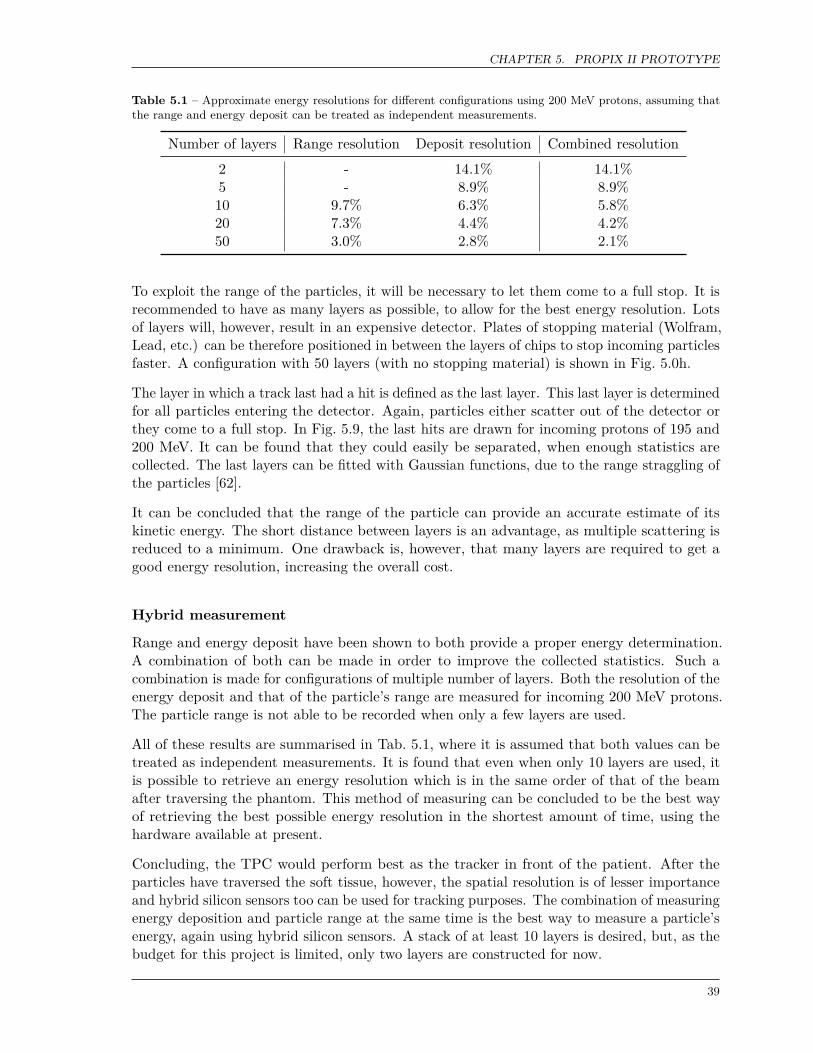
CHAPTER 5. PROPIX II PROTOTYPE
Table 5.1 – Approximate energy resolutions for different configurations using 200 MeV protons, assuming thatthe range and energy deposit can be treated as independent measurements.
Number of layers Range resolution Deposit resolution Combined resolution2 - 14.1% 14.1%5 - 8.9% 8.9%10 9.7% 6.3% 5.8%20 7.3% 4.4% 4.2%50 3.0% 2.8% 2.1%
To exploit the range of the particles, it will be necessary to let them come to a full stop. It isrecommended to have as many layers as possible, to allow for the best energy resolution. Lotsof layers will, however, result in an expensive detector. Plates of stopping material (Wolfram,Lead, etc.) can be therefore positioned in between the layers of chips to stop incoming particlesfaster. A configuration with 50 layers (with no stopping material) is shown in Fig. 5.0h.
The layer in which a track last had a hit is defined as the last layer. This last layer is determinedfor all particles entering the detector. Again, particles either scatter out of the detector orthey come to a full stop. In Fig. 5.9, the last hits are drawn for incoming protons of 195 and200 MeV. It can be found that they could easily be separated, when enough statistics arecollected. The last layers can be fitted with Gaussian functions, due to the range straggling ofthe particles [62].
It can be concluded that the range of the particle can provide an accurate estimate of itskinetic energy. The short distance between layers is an advantage, as multiple scattering isreduced to a minimum. One drawback is, however, that many layers are required to get agood energy resolution, increasing the overall cost.
Hybrid measurement
Range and energy deposit have been shown to both provide a proper energy determination.A combination of both can be made in order to improve the collected statistics. Such acombination is made for configurations of multiple number of layers. Both the resolution of theenergy deposit and that of the particle’s range are measured for incoming 200 MeV protons.The particle range is not able to be recorded when only a few layers are used.
All of these results are summarised in Tab. 5.1, where it is assumed that both values can betreated as independent measurements. It is found that even when only 10 layers are used, itis possible to retrieve an energy resolution which is in the same order of that of the beamafter traversing the phantom. This method of measuring can be concluded to be the best wayof retrieving the best possible energy resolution in the shortest amount of time, using thehardware available at present.
Concluding, the TPC would perform best as the tracker in front of the patient. After theparticles have traversed the soft tissue, however, the spatial resolution is of lesser importanceand hybrid silicon sensors too can be used for tracking purposes. The combination of measuringenergy deposition and particle range at the same time is the best way to measure a particle’senergy, again using hybrid silicon sensors. A stack of at least 10 layers is desired, but, as thebudget for this project is limited, only two layers are constructed for now.
39

CHAPTER 5. PROPIX II PROTOTYPE
Figure 5.10 – The simulated difference in numberof ionized electrons between a 200 MeV proton anda 546 keV electron.
Figure 5.11 – The simulated difference in thenumber of ionized electrons by a 200 MeV protonbetween the DME:CO2 (50:50) and Ar:CF4:CO2(45:40:15) gas mixtures.
5.2 GEM voltage scan
To arrive at an optimal detector performance, the voltages on the GEM foils are scanned toidentify the best settings. The best setting is defined here as the value in which the highestdata rate is obtained, whilst lowest amount of noise is present.
The total GEM-voltage is the sum of the three individual voltages on the GEM foils. Thesevoltages increase per foil in steps of 10 or 20V, with the highest voltage on the most upperGEM foil. This is the optimal way to run these devices according to the GEM-collaboration,as the ion back-flow is suppressed. The two used gas mixtures are Ar:CF4:CO2 (45:40:15),which is the mixture used in ProPix I, and DME:CO2 (50:50), which has been found to possesscharacteristics worth investigating. A transfer field of 2 kV/cm is used in the rest of this work.
The detector will be irradiated for ten seconds with a Sr-90 radioactive source, decaying as[63]:
9038Sr→90
39 Y + e− + νe (5.2)
To get a measure of the total number of ionised electrons, a simulation in Heed [64] is performed.Although the simulation does not predict the absolute number of electrons accurately, therelative difference can provide valuable insight into the physical possesses occurring.
The difference between ionisation by a 200 MeV proton and a 546 keV electron (from Sr-90)can be found in Fig. 5.10. It is clear that a high-energetic photon will produce more electronsthan a low-energetic electron as it traverses the chamber. The spatial resolution of tracksgenerated by a proton beam can therefore be expected to be better than tracks generated bythe radioactive source.
In Fig. 5.11, the two simulated gas-mixtures are drawn. It can be found that the differencebetween them is minimal. Both gasses can therefore be expected to perform comparable interms of spatial resolution, as they induce approximately the same number of electrons. Itshould, however, be noted that this simulation considers an ideal case in which no electroncapture is present. The individual characteristics should be carefully monitored.
40

CHAPTER 5. PROPIX II PROTOTYPE
a – The number of events with more than five clusters recorded in the detector. The distributions ofboth gasses flatten after reaching a certain value, because the gas is fully efficient.
b – The number of events with less than five clusters recorded in the detector. The distributions ofboth gasses spike after reaching a certain value, because of the GEM-discharges.
c – The signal-to-noise ratio, calculated by dividing the number of data events with the number ofnoise events. The highest values are found for VGAIN = 1280 V, for Ar:CF4:CO2 (45:40:15); andVGAIN = 1480 V, for DME:CO2 (50:50).
Figure 5.12 – Several properties for the different GEM-voltages in the Ar:CF4:CO2 (45:40:15) and DME:CO2(50:50) gas mixtures with irradiation by a Sr-90 source for 10 s.
41

CHAPTER 5. PROPIX II PROTOTYPE
Figure 5.13 – The hit distribution as a functionof the row number, for several points in time . Thet = 0 point is made at an arbitrary time of a fewminutes after starting up the configuration.
Figure 5.14 – The curvature of tracks inside thechamber. The white region is due to a malfunc-tioning area of the GEM foil.
The clustering algorithm from previous chapter is used to analyse the data. An event withmore than five clusters is treated as usable data; the rest is classified as noise. The data ofonly one chip is used, so that variations in collecting efficiency do not distort the results. Theobtained results on the data rate (Fig. 5.11a), the noise rate (Fig. 5.11b) and the resultingsignal-to-noise ratio (Fig. 5.11c) are given in their respective figures.
From the number of data events, it is evident that the detector detects more ionized electronsas the voltage on the GEMs is increased. The collection efficiency flattens when high voltagesare reached, implying that (almost) all electrons are collected. It is clear that the DME:CO2(50:50) gas-mixture requires a higher voltage to reach the same collection efficiencies. This isexpected, as the primary ionization of this mixture is lower than that of Ar:CF4:CO2 (45:40:15)[47].
When the gain-voltage is set to the lower region, it becomes more likely that an electroncoming from the source will result in less than five clusters. Thus, good events can incorrectlybe treated as noise in this case. It is however argued that no proper tracks can be constructedwith so few clusters, so the procedure can still be considered as accurate.
When the number of events with less than five clusters is concerned, jumps at approximately1300 and 1520 V are found for Ar:CF4:CO2 (45:40:15) and DME:CO2 (50:50), respectively.This increase is due to the spontaneous discharging of the GEM foil [65]. As the amplificationvoltage is turned up, more charge is collected on the isolating Kapton surface in between thecopper layers. This charge can randomly spark onto the chip, where it is detected as a signal.These sparks usually occur only once in an event, hence explaining the spike. Sparking shouldbe reduced to a minimum, as the detected charge has no physical basis and damage may occur
Combining above results, the signal-to-noise ratio can be calculated. The number of dataevents is simply divided by the number of noise events for this measurement.The highest signalsare found for VGAIN = 1280 for Ar:CF4:CO2 (45:40:15) and VGAIN = 1480 V for DME:CO2(50:50). These settings will be used in the remainder of this document.
42
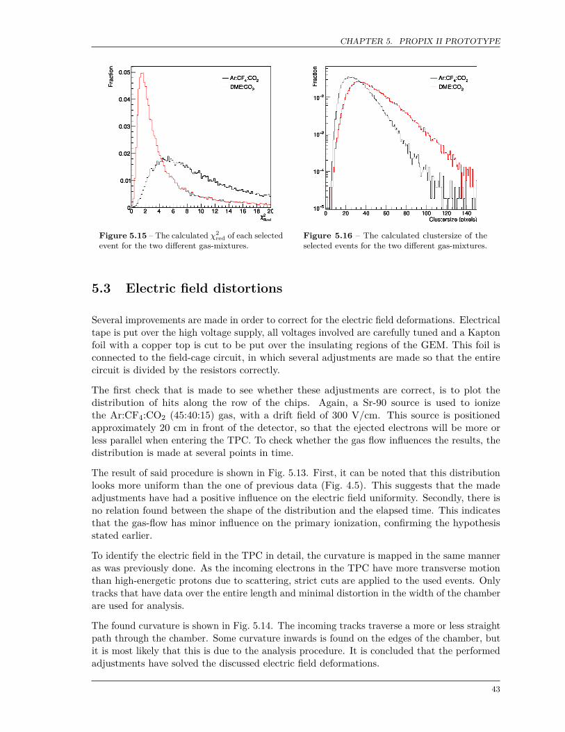
CHAPTER 5. PROPIX II PROTOTYPE
Figure 5.15 – The calculated χ2red of each selected
event for the two different gas-mixtures.Figure 5.16 – The calculated clustersize of theselected events for the two different gas-mixtures.
5.3 Electric field distortions
Several improvements are made in order to correct for the electric field deformations. Electricaltape is put over the high voltage supply, all voltages involved are carefully tuned and a Kaptonfoil with a copper top is cut to be put over the insulating regions of the GEM. This foil isconnected to the field-cage circuit, in which several adjustments are made so that the entirecircuit is divided by the resistors correctly.
The first check that is made to see whether these adjustments are correct, is to plot thedistribution of hits along the row of the chips. Again, a Sr-90 source is used to ionizethe Ar:CF4:CO2 (45:40:15) gas, with a drift field of 300 V/cm. This source is positionedapproximately 20 cm in front of the detector, so that the ejected electrons will be more orless parallel when entering the TPC. To check whether the gas flow influences the results, thedistribution is made at several points in time.
The result of said procedure is shown in Fig. 5.13. First, it can be noted that this distributionlooks more uniform than the one of previous data (Fig. 4.5). This suggests that the madeadjustments have had a positive influence on the electric field uniformity. Secondly, there isno relation found between the shape of the distribution and the elapsed time. This indicatesthat the gas-flow has minor influence on the primary ionization, confirming the hypothesisstated earlier.
To identify the electric field in the TPC in detail, the curvature is mapped in the same manneras was previously done. As the incoming electrons in the TPC have more transverse motionthan high-energetic protons due to scattering, strict cuts are applied to the used events. Onlytracks that have data over the entire length and minimal distortion in the width of the chamberare used for analysis.
The found curvature is shown in Fig. 5.14. The incoming tracks traverse a more or less straightpath through the chamber. Some curvature inwards is found on the edges of the chamber, butit is most likely that this is due to the analysis procedure. It is concluded that the performedadjustments have solved the discussed electric field deformations.
43
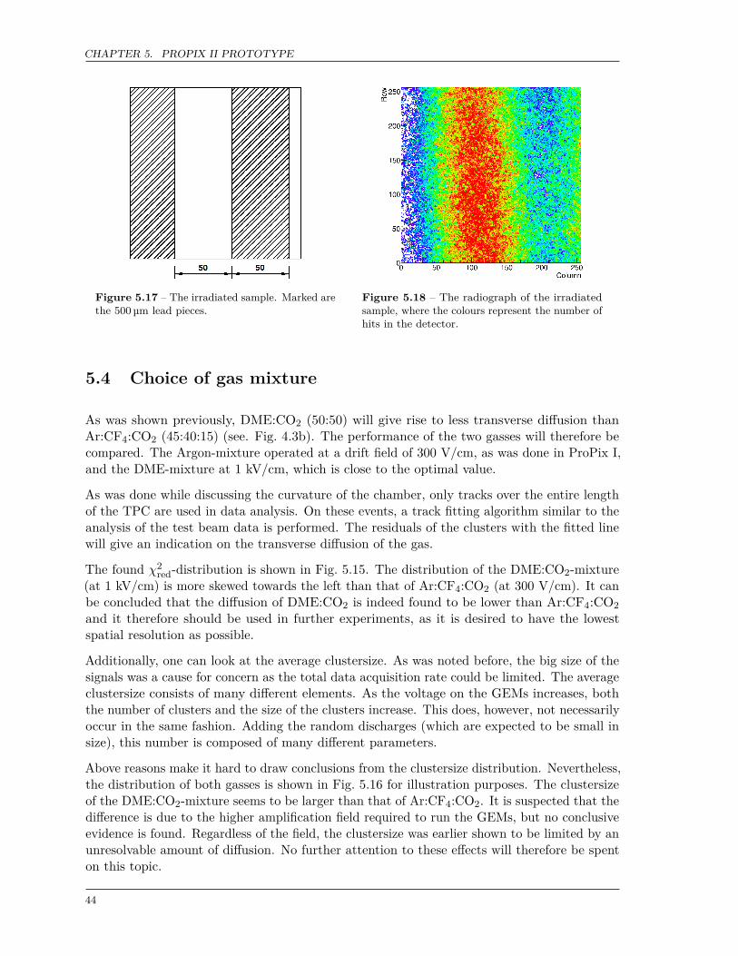
CHAPTER 5. PROPIX II PROTOTYPE
Figure 5.17 – The irradiated sample. Marked arethe 500 µm lead pieces.
Figure 5.18 – The radiograph of the irradiatedsample, where the colours represent the number ofhits in the detector.
5.4 Choice of gas mixture
As was shown previously, DME:CO2 (50:50) will give rise to less transverse diffusion thanAr:CF4:CO2 (45:40:15) (see. Fig. 4.3b). The performance of the two gasses will therefore becompared. The Argon-mixture operated at a drift field of 300 V/cm, as was done in ProPix I,and the DME-mixture at 1 kV/cm, which is close to the optimal value.
As was done while discussing the curvature of the chamber, only tracks over the entire lengthof the TPC are used in data analysis. On these events, a track fitting algorithm similar to theanalysis of the test beam data is performed. The residuals of the clusters with the fitted linewill give an indication on the transverse diffusion of the gas.
The found χ2red-distribution is shown in Fig. 5.15. The distribution of the DME:CO2-mixture
(at 1 kV/cm) is more skewed towards the left than that of Ar:CF4:CO2 (at 300 V/cm). It canbe concluded that the diffusion of DME:CO2 is indeed found to be lower than Ar:CF4:CO2and it therefore should be used in further experiments, as it is desired to have the lowestspatial resolution as possible.
Additionally, one can look at the average clustersize. As was noted before, the big size of thesignals was a cause for concern as the total data acquisition rate could be limited. The averageclustersize consists of many different elements. As the voltage on the GEMs increases, boththe number of clusters and the size of the clusters increase. This does, however, not necessarilyoccur in the same fashion. Adding the random discharges (which are expected to be small insize), this number is composed of many different parameters.
Above reasons make it hard to draw conclusions from the clustersize distribution. Nevertheless,the distribution of both gasses is shown in Fig. 5.16 for illustration purposes. The clustersizeof the DME:CO2-mixture seems to be larger than that of Ar:CF4:CO2. It is suspected that thedifference is due to the higher amplification field required to run the GEMs, but no conclusiveevidence is found. Regardless of the field, the clustersize was earlier shown to be limited by anunresolvable amount of diffusion. No further attention to these effects will therefore be spenton this topic.
44

CHAPTER 5. PROPIX II PROTOTYPE
5.5 Hybrid silicon sensor
As the material budget of the silicon sensor is relatively high, one needs a highly energeticparticle to test the performance of both. A Sr-90 electron will not be able to traverse a singlelayer. Cosmic particles could be used, but their rate is low and the entry position on thesensor not well defined. Therefore, it has not been possible to do a detailed analysis of thesensors performance.
However, in order to show that all components are behaving as expected, a simple radiographis constructed. The Sr-90 is again positioned above the sensor. Between the sensor and theradioactive source, a plate of 500 µm lead in thickness - enclosed with a few millimetre ofplastic - is placed. Holes in this plate are present in order to show the difference in materialdensity. The dimensions of said phantom can be found in Fig. 5.17.
The reaction of the hybrid silicon sensor after irradiation is shown in Fig. 5.18, where thecolours represent the number of hits in the chip. It can be found that the expected shape isretrieved with some precision. Once again, scattering of the particles reduces the image quality.For more characterisation on e.g. spatial and energy resolution, tests at a proton beam shouldbe performed.
45


6 | Conclusion and outlook
Through a literature study it was shown that the proton radiography prototypes underdevelopment by other groups have major interference with the particle beam and are physicallylimited in their data-acquisition rate. To take proton radiography to the level required forclinical application, new detector configurations must be investigated. A design consisting of asingle TPC and several hybrid silicon sensors was shown to possess the intrinsic propertiesrequired for a competitive detector and was therefore further investigated.
The study of ProPix II started with the investigation of the previously constructed design -ProPix I. Using the data collected at the proton beam at KVI, Groningen, it was first shownhow the electric field inside the TPC carried multiple deformations. Through simulations it wasfound that these problems arose due to a combination of incorrectly voltages, an unshieldedHV-supply cable and a missing guard ring. Additionally, it was shown how the diffusion ofelectrons in the gas between the GEM foils could cause the large clustersize.
Following these physical investigations, several steps in data preparation have been performed.A clustering algorithm was created in to reduce the effect of large signals and an offsetcorrection was made to retrieve more straight tracks. Radiographs using two independentreconstructions were shown afterwards: one by measuring the particles residual energy, whichwas determined to carry a density resolution in the order of 2.5%; the other by measuring themultiple scattering magnitude, which is shown for the first time with the discussed detectorand is very promising. The combination of both signals provides a proper method of separatingdifferent materials and deserves further investigation.
With all information from ProPix I collected, the ProPix II design was proposed. Extensivesimulations studies showed that a design with a TPC as tracker has significantly less beaminterference in comparison with silicon sensors. If the particles have traversed the phantom,however, the spatial resolution is of lesser importance and the silicon sensors too can be usedfor tracking purposes. Through the investigation of several measurement techniques, it wasshown that the simultaneous measurement of a particle’s energy deposit and range providesthe best energy resolution.
A configuration with two detecting planes was constructed, serving as a proof of principle forabove method. These planes remain to be fully characterised at a test beam, as the optionsfor testing at the lab are limited. The TPC was adjusted in several ways: the voltages werecarefully tuned, electric tape was placed over the HV-cable and a guard ring was designed forthe circuit. Irradiation tests with a Sr-90 source showed that these additions solved the electricfield deformations. Following this, the optimal settings for GEM voltages were determinedand the effect of gas choice on the results was shown.
47

CHAPTER 6. CONCLUSION AND OUTLOOK
Before testing the ProPix II assembly with highly energetic protons, several components shouldbe further investigated. First of all, the GEM foils should ideally be replaced by anotheramplification device. It was shown that the large clustersize cannot be resolved, as the diffusionbetween layers is limiting. Several projects in the R&D-department of Nikhef on the topicof electron multiplication are ongoing, of which GridPix [66] is the best candidate for futuredetector designs. GridPix is, however, much more sensitive to sparks, which makes the detectormore fragile.
As for the choice of gas, it was shown that DME:CO2 (50:50) gas has better performancethan Ar:CF4:CO2 (45:40:15) in terms of track resolution. Other studies have similarly shownthe great promise of said mixture, but also make notes on unwanted effects [67, 68]. Theflammability of the mixture [69], for instance, makes large experiments reluctant to use this gasin their chambers. This work similarly finds an undesired low amount of primary ionization ofthe gas. Still, it is argued that DME:CO2 (50:50) should be used in future detector experiments,as the advantages outweigh the disadvantages.
The electric field inside the TPC is not a limiting factor in terms of track resolution. TheKapton-copper foil works sufficient and can be used in further detector designs. After theelectric field was tuned through the several modifications, the major distortions are absent.Smaller distortions may easily be resolved by performing an offset procedure in the analysis.As a resolution below 1 mm is not required for a functional proton radiography device, nofurther attention needs to be spent on this topic.
The combination of measuring Time of Arrival and Time over Threshold in the Timepix3chip has been shown to work great. If one considers an active volume of approximately 3 x 3cm2, a detector built with GridPix-technology will generate approximately 100 hits [70]. Asthe SPIDR read-out system can sustain 80 x 106 hits per/s, a rate of 0.8 MHz is feasible. Aslightly smaller detector or a reduced flow of ionizing gas can push the rate over the required 1MHz for proton radiography. In later stages, the possibility of detecting multiple particles atonce can be studied.
The detector size remains an open issue. The TPC height is limited by the total time theelectrons need to drift downwards, which cannot be too large as this will limit the protonmeasurement frequency. The hybrid detecting planes are limited by the size of the chips, whichcannot be enlarged easily. Some effort needs to be spent to look into configurations whichuse several sub-detectors, whilst keeping dead area to a minimum. A change to a 1 x 4 chipdesign and making a common cathode are a few of the options available [5].
As track resolution and detector speed are close to the requirements for clinical application, itwill start to become necessary to look into material reconstruction algorithms. These processeshave been studied in depth in regard to CT-scans, but designs for proton radiography are onlystarting up [71]. Different from CT, there needs to be careful consideration on the method oftreating particles that scatter away from the detector.
Concluding, all ingredients are present in order to build a full scale detector prototype whichcan be tested in a clinical setting. The speed of the ProPix II system should pass the 1 MHzbenchmark, the spatial resolution of less than 1 mm has been achieved, the active area canbe improved by making modular designs and the density resolution is with 2.5% close tothe required 1%. ProPix II should be tested at a proton beam to make sure that all madeadjustments are fully functional, but this stage does not need to take a lot of time. Hopefully,proton radiography will soon be able to contribute in the ongoing fight against cancer.
48

Bibliography
[1] S. W. Steward and C. P. Wild. World Cancer Report 2014. WHO Press, 2014.
[2] D. Schardt, T. Elsasser, and D. Schulz-Ertner. Heavy-ion tumor therapy: Physical and radiobiolo-gical benefits. Rev. Mod. Phys., 82:383–425, Feb 2010.
[3] B. Schaffner and E. Pedroni. The precision of proton range calculations in proton radiotherapytreatment planning: experimental verification of the relation between CT-HU and proton stoppingpower. Phys. Med. Biol., 43(6):1579–1592, 1998.
[4] P. Radaelli. Proton Radiography with a Timepix3 based Gaseous Tracking Detector. Master’sthesis, VU University Amsterdam, 2015.
[5] N. Van der Weiden. Building and Testing a GEM-based Time Projection Chamber for ProtonRadiography. Master’s thesis, VU University Amsterdam, 2015.
[6] S. R. Cherry, J. A. Sorenson, and M. E. Phelps. Physics in Nuclear Medicine. Elsevier, 2003.
[7] J. Beringer et al. Passage of Particles through Matter. Phys. Rev. D86, 2013.
[8] C. Leroy and P-G. Rancoita. Principles of Radiation Interation in Matter and Detection. WorldScientific Publishing Company, 2009.
[9] M. J. Berger et al. Stopping-power and range tables for electrons, protons, and helium ions. NISTPhysics Laboratory, 1998.
[10] F. M. Khan. Khan’s the physics of radiation therapy. Lippincott Williams & Wilkins, 2014.
[11] J. Locke et al. Radiotherapy for epithelial skin cancer. International Journal of Radiation Oncology*Biology* Physics, 51(3):748–755, 2001.
[12] Sumitomo Heavy Industries. http://www.shi.co.jp/quantum/eng/product/proton/proton.html. [Accessed 1-June-2016].
[13] M. K. Bucci, A. Bevan, and M. Roach. Advances in radiation therapy: conventional to 3D, toIMRT, to 4D, and beyond. CA: a cancer journal for clinicians, 55(2):117–134, 2005.
[14] G. T. Herman. Fundamentals of computerized tomography: image reconstruction from projections.Springer Science & Business Media, 2009.
[15] R. W. Brown et al. Magnetic resonance imaging: physical principles and sequence design. JohnWiley & Sons, 2014.
[16] D. L. Bailey et al. Positron emission tomography. Springer, 2005.
[17] M. Witt et al. Optimization of the stopping-power-ratio to Hounsfield-value calibration curve inproton and heavy ion therapy. Zeitschrift für Medizinische Physik, 25(3):251–263, 2015.
49

BIBLIOGRAPHY
[18] U. Schneider and E. Pedroni. Proton radiography as a tool for quality control in proton therapy.Med. Phys., 22(4):356–363, 1995.
[19] G. R. Lynch and O. I. Dahl. Approximations to multiple Coulomb scattering. Nuclear Instrumentsand Methods in Physics Research Section B: Beam Interactions with Materials and Atoms, 58(1):6–10, 1991.
[20] Ministerie van Volksgezondheid Welzijn en Sport. Regeling protonentherapie. https://zoek.officielebekendmakingen.nl/stcrt-2013-22203. [Accessed 1-June-2016].
[21] R. Schulte et al. Conceptual design of a proton computed tomography system for applications inproton radiation therapy. IEEE Transactions on Nuclear Science, 51(3):866–872, 2004.
[22] M. A Weinstein, P. M. Duchesneau, and W. J. MacIntyre. White and Gray Matter of the BrainDifferentiated by Computed Tomography. Radiology, 122(3):699–702, 1977.
[23] U. Amaldi et al. Construction, test and operation of a proton range radiography system. NuclearInstruments and Methods in Physics Research Section A: Accelerators, Spectrometers, Detectorsand Associated Equipment, 629(1):337 – 344, 2011.
[24] G. Poludniowski, N. M. Allinson, and P. M. Evans. Proton radiography and tomography withapplication to proton therapy. The British journal of radiology, 88(1053):20150134, 2015.
[25] D. Presti et al. A real-time, large area, high space resolution particle radiography system. Journalof Instrumentation, 9(06):C06012, 2014.
[26] G. Coutrakon et al. A New Proton CT Scanner. 2014.
[27] H.F-W. Sadrozinski et al. Development of a head scanner for proton CT. Nuclear Instrumentsand Methods in Physics Research Section A: Accelerators, Spectrometers, Detectors and AssociatedEquipment, 699:205–210, 2013.
[28] R.P. Johnson et al. Results of a pre-clinical head scanner for proton CT. In IEEE Nuclear ScienceSymposion and Medical Imaging Conference, 2014.
[29] Y. Saraya et al. Study of spatial resolution of proton computed tomography using a siliconstrip detector. Nuclear Instruments and Methods in Physics Research Section A: Accelerators,Spectrometers, Detectors and Associated Equipment, 735:485–489, 2014.
[30] V. Sipala et al. PRIMA: An apparatus for medical application. Nuclear Instruments and Methodsin Physics Research Section A: Accelerators, Spectrometers, Detectors and Associated Equipment,658(1):73–77, 2011.
[31] J. T. Taylor et al. Proton tracking for medical imaging and dosimetry. Journal of Instrumentation,10(02):C02015, 2015.
[32] M. Scaringella et al. A proton Computed Tomography based medical imaging system. Journal ofInstrumentation, 9(12):C12009, 2014.
[33] P. Pemler et al. A detector system for proton radiography on the gantry of the Paul-Scherrer-Institute. Nuclear Instruments and Methods in Physics Research Section A: Accelerators, Spectro-meters, Detectors and Associated Equipment, 432(2):483–495, 1999.
[34] W. Blum, W. Riegler, and L. Rolandi. Particle detection with drift chambers. Springer Science &Business Media, 2008.
[35] C.H. Hahn et al. Apparatus for digital imaging photodetector using Gas Electron Multiplier,February 16 2010. US Patent 7,663,081.
[36] S.D. Pringle. Gas Electron Multiplier detector, October 23 2012. US Patent 8,294,088.
50

BIBLIOGRAPHY
[37] F. Sauli. GEM: A new concept for electron amplification in gas detectors. Nuclear Instrumentsand Methods in Physics Research Section A: Accelerators, Spectrometers, Detectors and AssociatedEquipment, 386(2):531–534, 1997.
[38] M. Schut. Characterisation of the Timepix3 chip using a gaseous detector. Master’s thesis,University of Amsterdam, 2015.
[39] R. Ballabriga. The Design and Implementation in 0.13µm CMOS of an Algorithm PermittingSpectroscopic Imaging with High Spatial Resolution for Hybrid Pixel Detectors. PhD thesis, CERN,2009.
[40] T. Poikela et al. Timepix3: a 65K channel hybrid pixel readout chip with simultaneous ToA/ToTand sparse readout. Journal of Instrumentation, 9(05):C05013, 2014.
[41] J. Visser et al. SPIDR: a read-out system for Medipix3 & Timepix3. Journal of Instrumentation,10(12):C12028, 2015.
[42] R. Novotny. Performance of the BaF2-calorimeter TAPS. Nuclear Physics B-Proceedings Supple-ments, 61(3):137–142, 1998.
[43] CAEN. Desktop Digitizers. http://caen.it. [Accessed 1-June-2016].
[44] E. R. Van der Graaf et al. AGORFIRM, the AGOR facility for irradiations of materials. InRadiation and Its Effects on Components and Systems (RADECS), 2009 European Conference on,pages 451–454. IEEE, 2009.
[45] R. Veenhof et al. Garfield, a drift chamber simulation program. In International Conference onProgramming and Mathematical Methods for Solving Physical Problems, Dubna, Russia, pages14–19, 1993.
[46] S. Biagi. Magboltz-transport of electrons in gas mixtures. CERN program library, 2005.
[47] A. Sharma and R. Veenhof. Properties of some gas mixtures used in tracking detectors. SLACJournal, ICFA, 16, 1998.
[48] George S.P. et al. Measurement of an accelerator based mixed field with a Timepix detector.Journal of Instrumentation, 10(03):P03005, 2015.
[49] C. Hasterok. GEM Simulation Studies, 2011. Summer Student Report.
[50] H. Jasak, A. Jemcov, and Z. Tukovic. OpenFOAM: A C++ library for complex physics simulations.In International workshop on coupled methods in numerical dynamics, volume 1000, pages 1–20,2007.
[51] J. Ahrens et al. ParaView: An End-User Tool for Large-Data Visualization, 2005.
[52] C. Geuzaine and J-F. Remacle. Gmsh: A 3-D finite element mesh generator with built-inpre-and post-processing facilities. International Journal for Numerical Methods in Engineering,79(11):1309–1331, 2009.
[53] M. Lyly, J. Ruokolainen, and E. Järvinen. ELMER - a finite element solver for multiphysics.CSC-report on scientific computing, 2000:156–159, 1999.
[54] Imaging Equipment Ltd. Tissue Equivalent Materials Gammex. http://www.imagingequipment.co.uk. [Accessed 1-June-2016].
[55] Agostinelli, S. and others. GEANT4: A Simulation toolkit. Nucl. Instrum. Meth., A506:250–303,2003.
[56] H. Paganetti. Proton therapy physics. CRC Press, 2011.
[57] V. Gromov et al. Development and applications of the Timepix3 readout chip. PoS, VER-TEX2011:046, 2011.
51
BIBLIOGRAPHY
[58] Nikhef. Timepix3 QUAD board schematics, 2014.
[59] E. Frojdh et al. Timepix3: first measurements and characterization of a hybrid-pixel detectorworking in event driven mode. Journal of Instrumentation, 10(01):C01039, 2015.
[60] S. Guatelli et al. Geant4 Anthropomorphic Phantoms. In 2006 IEEE Nuclear Science SymposiumConference Record, volume 3, pages 1359–1362, 2006.
[61] NIST. Material database. http://physics.nist.gov/cgi-bin/Star/compos.pl?matno=262.[Accessed 1-June-2016].
[62] W. Wieszczycka and W. H. Scharf. Proton radiotherapy accelerators. world scientific, 2001.
[63] E. Browne, R. B. Firestone, and V. S. Shirley. Table of radioactive isotopes. 1986.
[64] I. B. Smirnov. Heed C++. http://ismirnov.web.cern.ch/ismirnov/heed. [Accessed 1-June-2016].
[65] S. Bachmann et al. Discharge studies and prevention in the gas electron multiplier (GEM). NuclearInstruments and Methods in Physics Research Section A: Accelerators, Spectrometers, Detectorsand Associated Equipment, 479(203):294 – 308, 2002.
[66] H. Van der Graaf et al. The GridPix detector: History and perspective. Mod. Phys. Lett.,A28:1340021, 2013.
[67] W. J. C. Koppert. GridPix: development and characterisation of a gaseous tracking detector. PhDthesis, University of Amsterdam, 2015.
[68] M. Fransen. Gridpix: TPC development on the right track. The development and characterisationof a TPC with a CMOS pixel chip read out. PhD thesis, University of Amsterdam, 2012.
[69] European Biofuels Technology Platform. Dimethyl ether (DME) Fact Sheet . http://www.biofuelstp.eu/factsheets/dme-fact-sheet.html. [Accessed 1-June-2016].
[70] B. F. B. Huisman. Proton Imaging with Gridpix Detectors. Master’s thesis, University ofAmsterdam, 2012.
[71] S. N. Penfold et al. Total variation superiorization schemes in proton computed tomography imagereconstruction. Medical physics, 37(11):5887–5895, 2010.
52