Proton Radiation Belt Remediation (PRBR)

Presentation to Review Committee Dennis Papadopoulos

Tom Wallace

October 28, 2008

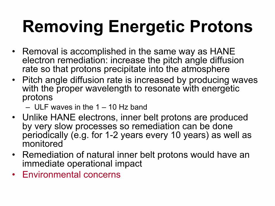
Removing Energetic Protons •  Removal is accomplished in the same way as HANE

electron remediation: increase the pitch angle diffusion rate so that protons precipitate into the atmosphere

•  Pitch angle diffusion rate is increased by producing waves with the proper wavelength to resonate with energetic protons –  ULF waves in the 1 – 10 Hz band

•  Unlike HANE electrons, inner belt protons are produced by very slow processes so remediation can be done periodically (e.g. for 1-2 years every 10 years) as well as monitored

•  Remediation of natural inner belt protons would have an immediate operational impact

•  Environmental concerns

Proton Effects on Commercial Electronics

•  Higher LEO Orbits: commercial electronics are regularly affected by proton upsets

•  Lower LEO Orbits: affected during SAA transits and at high latitudes

•  Example: IBM PowerPC 603 in Iridium (0.5 micron CMOS) – cache had to be disabled because of upsets caused by SAA

Proton Effects Scaling with Feature Size

•  As commercial feature sizes scale down, proton upsets will become much more frequent

•  Critical charge for upset scales as (feature size)2

•  For large feature sizes, protons cause upsets by hitting nuclei and releasing secondary particles that deposit charge

•  At 65 nm and smaller, a proton deposits enough charge in silicon to cause an upset directly

•  This can increase the proton SEU cross section by 2-3 orders of magnitude for deep submicron devices

•  Major issue for micro-satellites

IS PRBR A SOLUTION – ARE THERE ENVIRONMENTAL EFFECTS

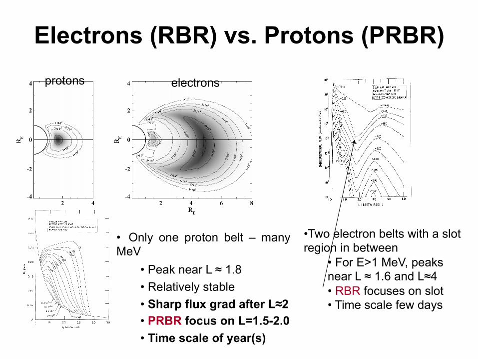
Electrons (RBR) vs. Protons (PRBR) protons electrons

•  Only one proton belt – many MeV

•  Peak near L ≈ 1.8 •  Relatively stable •  Sharp flux grad after L≈2 •  PRBR focus on L=1.5-2.0 •  Time scale of year(s)

• Two electron belts with a slot region in between

•  For E>1 MeV, peaks near L ≈ 1.6 and L≈4 •  RBR focuses on slot •  Time scale few days

Proton Lifetime in the Inner RB

26 years Steady State à Source = Loss

4 1.3 32 10 ( / ) (# / ) yearsT E MeV cm ρ≈ × < >

55 MeV

Loss à Slowing down by exciting and ionizing electrons in the thermosphere

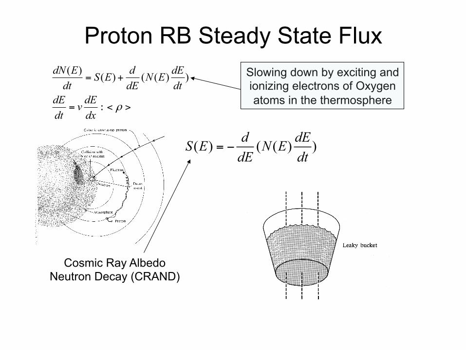
Proton RB Steady State Flux Slowing down by exciting and ionizing electrons of Oxygen atoms in the thermosphere

( ) ( ) ( ( ) )dN E d dES E N Edt dE dt

dE dEvdt dx

ρ

= +

= < >:

Cosmic Ray Albedo Neutron Decay (CRAND)

( ) ( ( ) )d dES E N EdE dt

= −

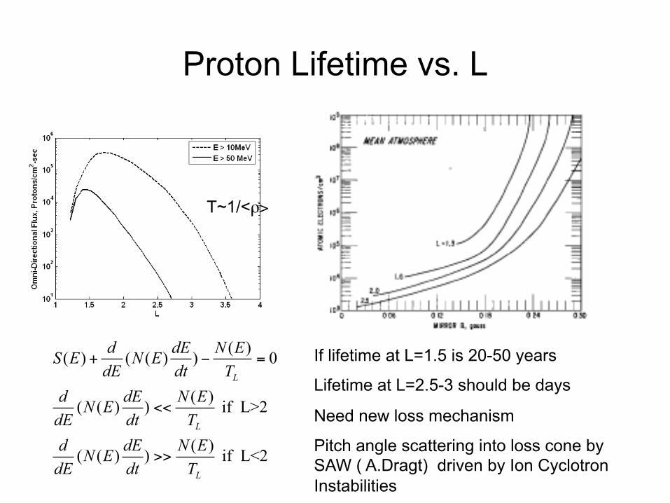
Proton Lifetime vs. L

( )( ) ( ( ) ) 0

( )( ( ) ) if L>2

( )( ( ) ) if L<2

L

L

L

d dE N ES E N EdE dt T

d dE N EN EdE dt Td dE N EN EdE dt T

+ − =

<<

>>

If lifetime at L=1.5 is 20-50 years

Lifetime at L=2.5-3 should be days

Need new loss mechanism

Pitch angle scattering into loss cone by SAW ( A.Dragt) driven by Ion Cyclotron Instabilities

T~1/<ρ>

Pitch Angle Diffusion (PAD) at high L

z z

z z

k vk vω − = ±Ω

≈ΩSAW

Enhance proton loss rate in the inner RB by PAD on artificially generated and injected SAW

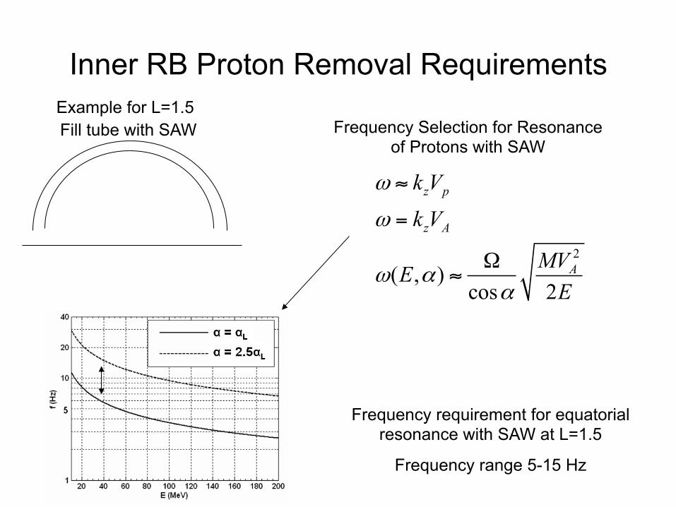
Inner RB Proton Removal Requirements Example for L=1.5

2

( , )cos 2

z p

z A

A

k Vk V

MVEE

ω

ω

ω αα

≈

=

Ω≈

Frequency Selection for Resonance of Protons with SAW

Fill tube with SAW

Frequency requirement for equatorial resonance with SAW at L=1.5

Frequency range 5-15 Hz

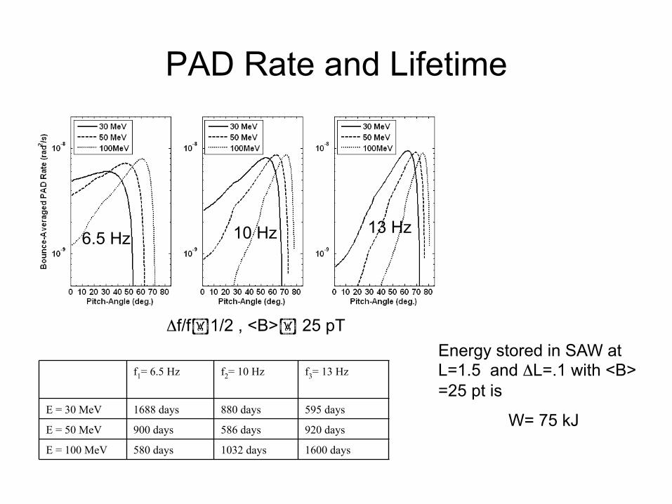
PAD Rate and Lifetime

Δf/f1/2 , <B> 25 pT

6.5 Hz 10 Hz 13 Hz

f1= 6.5 Hz f2= 10 Hz f3= 13 Hz

E = 30 MeV 1688 days 880 days 595 days E = 50 MeV 900 days 586 days 920 days E = 100 MeV 580 days 1032 days 1600 days

Energy stored in SAW at L=1.5 and ΔL=.1 with <B> =25 pt is

W= 75 kJ

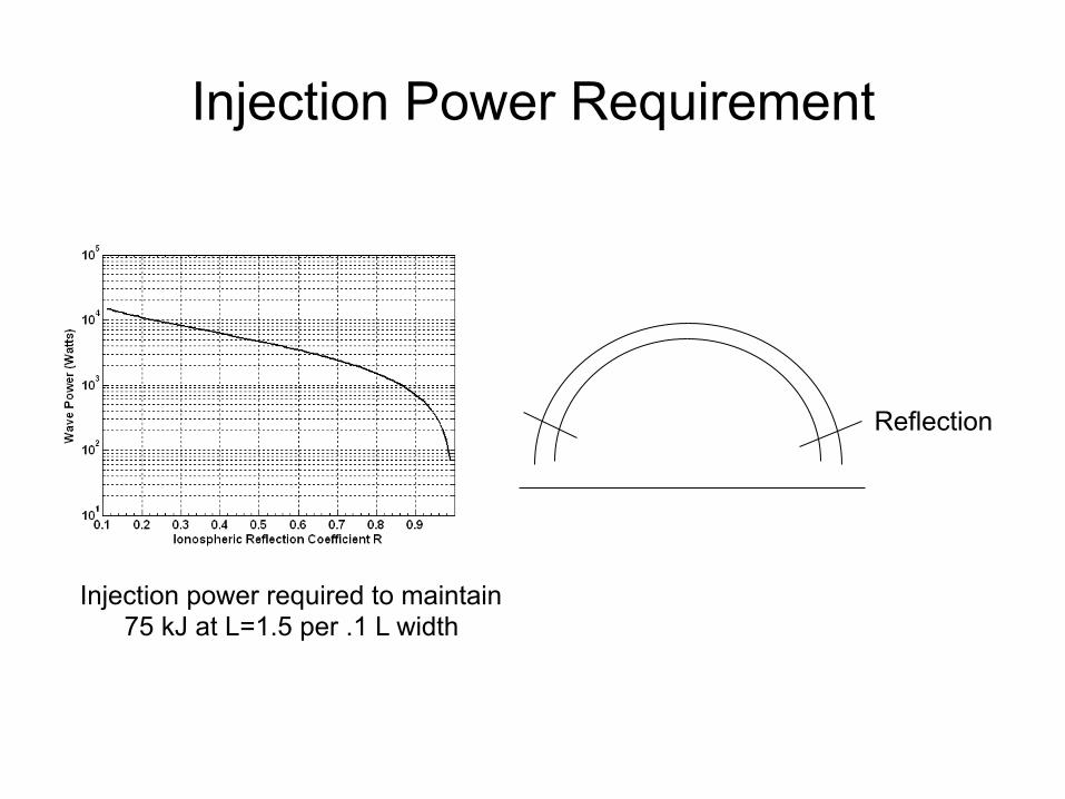
Injection Power Requirement

Reflection

Injection power required to maintain 75 kJ at L=1.5 per .1 L width

How to Get these Waves - Ground-based Transmitter Options

•  Initial estimates indicate that less than kWatt level of ULF injected into the L = 1.5-1.8 region is required to get interesting removal lifetime

•  What does it take to get it •  There are a number of potential options:

–  Conventional ULF/ELF transmitters (grounded dipoles) –  Rotating electromagnets (conventional and low and high temperature

superconducting) –  Space based rotating magnets or neutral gas injection –  Electrojet-free F-region ionospheric heating

•  Present estimates for the first two

<b> 75 km

120 km

A≈1010 m2

B p=IL

δ

R

skin depth

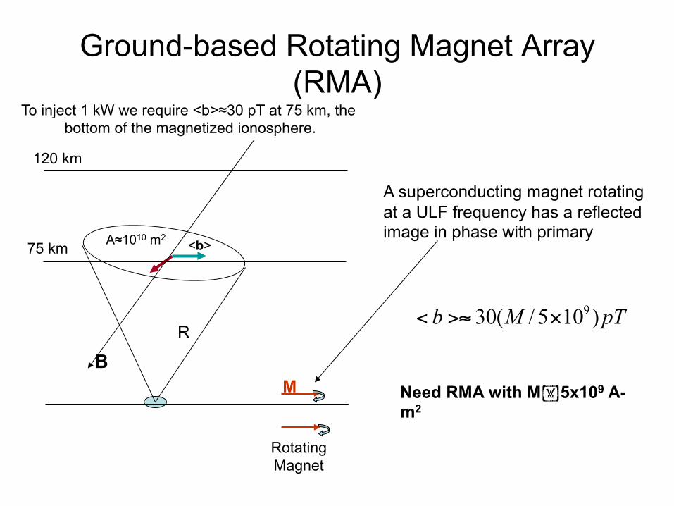
To inject 1 kW we require <b>≈30 pT at 75 km, the bottom of the magnetized ionosphere.

HMD

Ground-based Conventional Transmitter - HED

Conventional ULF/ELF sources (like Sanguine/Seafarer) are grounded wires – HED (Jason Study by Perkins et al.)

2 10 2 1060( / 2 10 )[ ] 30( / 2 10 )2( )

b IL pT IL pTLδδ

< >≈ × ≈ ×+

Need MIL2 2x1010 A-m2

Traditional HED Sources

~ Δ

Plane view of HED antenna

2

2( )effIlMlδδ

=+

3 3

12 (1 / )

effM IlBh h l

µ δµ

δ≈ ≈

+

1/ 2 2 1/ 2 1/ 2

2 10 1/ 2 2 1/ 2 5/ 2 2

3.3( / ) ( /10 ) ( / ) kAIL 2 10 ( / ) ( /10 ) ( / 2 )I P MW L km

P MW L km A mσ

σ

−

−

=

= × −

Jason study Perkins et al.

<b> 75 km

120 km

A≈1010 m2

B R

To inject 1 kW we require <b>≈30 pT at 75 km, the bottom of the magnetized ionosphere.

Ground-based Rotating Magnet Array (RMA)

A superconducting magnet rotating at a ULF frequency has a reflected image in phase with primary

930( / 5 10 )b M pT< >≈ ×

Need RMA with M5x109 A-m2

Rotating Magnet

M

Innovative Sources: Rotating Magnets

•  Rotating superconducting magnets are useful for frequencies of up to 10 Hz

•  They are compact sources of large moments and can be used in arrays

•  Example design: –  Superconducting coil 5 m high x 5 m wide x 5 m long –  25 m2 area –  100 Amps DC current –  4×104 turns –  M = 108 A-m2 per coil, meaning 50 coils are needed

•  Cost estimate: ~$1M/coil –  LTS wire at $2/kA-m: $160k/coil –  Dewar and refrigeration: $500k/coil (assuming LHe large plant shared

across dozens of coils) –  Mechanical rotation: $300k/coil (depends strongly on maximum

frequency)

Removing Energetic Protons •  Removal is accomplished in the same way as HANE

electron remediation: increase the pitch angle diffusion rate so that protons precipitate into the atmosphere

•  Pitch angle diffusion rate is increased by producing waves with the proper wavelength to resonate with energetic protons –  ULF waves in the 1 – 10 Hz band

•  Unlike HANE electrons, inner belt protons are produced by very slow processes so remediation can be done periodically (e.g. for 1-2 years every 10 years) as well as monitored

•  Remediation of natural inner belt protons would have an immediate operational impact

•  Similar ULF system could potentially be used for MeV electrons

Environmental Effects of Energetic Proton Precipitation in Middle Atmosphere

Solar Proton (SPE) Events associated with CMEs

Flux of > 10 MeV protons >104 #/cm2 sec Leads to 20% variation of Ozone in middle atmosphere (40-50 km) with recovery time of week

Jackman et al. JGR,1995

Verronen et al JGR, 2005 Noise for E>10 MeV 10 #/cm2sec

Environmental Issues – Effects in the Stratosphere – Ozone Loss

PRBR precipitation flux

L=1.5-2

Precipitation area 1017 cm2

Proton inventory 1023-1024

Assume all particles precipitate over one year

Proton flux in atmosphere

<1 #/cm2 sec

Smaller than noise

Environmental Effects - Magnetic

•  Diamagnetic current due to Inner Belt protons << Ring Current

•  Magnetic Moment of Ring Current <<Magnetic Moment of Earth (7x1021A-m2)

•  Magnetic effect from PRBR nrgligible