Proteus: agile ML elasticity through tiered reliabilityin dynamic resource markets

Aaron Harlap§ Alexey Tumanov† Andrew Chung§

Gregory R. Ganger§ Phillip B. Gibbons§

§Carnegie Mellon University †UC Berkeley

AbstractMany shared computing clusters allow users to utilize ex-

cess idle resources at lower cost or priority, with the provisothat some or all may be taken away at any time. But, exploit-ing such dynamic resource availability and the often fluc-tuating markets for them requires agile elasticity and effec-tive acquisition strategies. Proteus aggressively exploits suchtransient revocable resources to do machine learning (ML)cheaper and/or faster. Its parameter server framework, Ag-ileML, efficiently adapts to bulk additions and revocationsof transient machines, through a novel 3-stage active-backupapproach, with minimal use of more costly non-transientresources. Its BidBrain component adaptively allocates re-sources from multiple EC2 spot markets to minimize aver-age cost per work as transient resource availability and costchange over time. Our evaluations show that Proteus reducescost by 85% relative to non-transient pricing, and by 43%relative to previous approaches, while simultaneously reduc-ing runtimes by up to 37%.

1. IntroductionStatistical machine learning (ML) has become a primary

data processing activity for business, science, and onlineservices that attempt to extract insight from observation(training) data. Generally speaking, ML algorithms itera-tively process training data to determine model parametervalues that make an expert-chosen statistical model best fit it.Once fit (trained), such models can predict outcomes for newdata items based on selected characteristics (e.g., for recom-mendation systems), correlate effects with causes (e.g., forgenomic analyses of diseases), label new media files (e.g.,which ones are funny cat videos?), and so on.

ML model training is often quite resource intensive, re-quiring hours on 10s or 100s of cores to converge on a solu-tion. As such, it should exploit any available extra resourcesor cost savings. Many modern compute infrastructures offer

Permission to make digital or hard copies of all or part of this work for personal or classroom use is granted withoutfee provided that copies are not made or distributed for profit or commercial advantage and that copies bear this noticeand the full citation on the first page. Copyrights for components of this work owned by others than the author(s) mustbe honored. Abstracting with credit is permitted. To copy otherwise, or republish, to post on servers or to redistribute tolists, requires prior specific permission and/or a fee. Request permissions from permissions@acm.org.

EuroSys ’17, April 23 - 26, 2017, Belgrade, Serbia

c© 2017 Copyright held by the owner/author(s). Publication rights licensed to ACM.ISBN 978-1-4503-4938-3/17/04. . . 5.00

DOI: http://dx.doi.org/10.1145/3064176.3064182

0

20

40

60

80

100

120

Cos

t ($)

0

1

2

3

Tim

e (H

rs)

CostRunTime

All On- Demand

Standard + Checkpointing Proteus

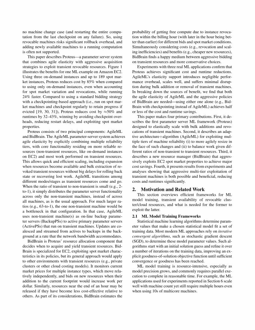
Figure 1: Cost and time benefits of Proteus. This graph showsaverage cost (left axis) and runtime (right axis) for running theMLR application (see Section 6.2) on the AWS EC2 US-EAST-1 Region. The three configurations shown are: 128 on-demandmachines, using 128 spot market machines with checkpoint/restartfor dealing with evictions and a standard strategy of bidding the on-demand price, and Proteus using 3 on-demand and up to 189 spotmarket machines. Proteus reduces cost by 85% relative to using allon-demand machines and by ≈50% relative to the checkpointing-based scheme. Full experimental details can be found in Section 6.

a great opportunity: transient availability of cheap but revo-cable resources. For example, Amazon EC2’s spot marketand Google Compute Engine’s preemptible instances oftenallow customers to use machines at a 70–80% discount [2]off the regular price, but with the risk that they can be takenaway at any time. Many cluster schedulers similarly allowlower-priority jobs to use resources provisioned but not cur-rently needed to support business-critical activities, takingthe resources away when those activities need them. MLmodel training could often be faster and/or cheaper by ag-gressively exploiting such revocable resources.

Unfortunately, efficient modern frameworks for parallelML, such as TensorFlow [6], MxNet [9], and Petuum [37],are not designed to exploit transient resources. Most usea parameter server architecture, in which parallel work-ers process training data independently and use a special-ized key-value store for shared state, offloading communi-cation and synchronization challenges from ML app writ-ers [10, 22, 25]. Like MPI-based HPC applications, theseframeworks generally assume that the set of machines isfixed, optimizing aggressively for the no machine failure and

no machine change case (and restarting the entire compu-tation from the last checkpoint on any failure). So, usingrevocable machines risks significant rollback overhead, andadding newly available machines to a running computationis often not supported.

This paper describes Proteus—a parameter server systemthat combines agile elasticity with aggressive acquisitionstrategies to exploit transient revocable resources. Figure 1illustrates the benefits for one ML example on Amazon EC2.Using three on-demand instances and up to 189 spot mar-ket instances, Proteus reduces cost by 85% when comparedto using only on-demand instances, even when accountingfor spot market variation and revocations, while running24% faster. Compared to using a standard bidding strategywith a checkpointing-based approach (i.e., run on spot mar-ket machines and checkpoint regularly to retain progress ifevicted [19, 30, 31]), Proteus reduces cost by ≈50% andruntimes by 32–43%, winning by avoiding checkpoint over-heads, reducing restart delays, and exploiting spot marketproperties.

Proteus consists of two principal components: AgileMLand BidBrain. The AgileML parameter-server system achievesagile elasticity by explicitly combining multiple reliabilitytiers, with core functionality residing on more reliable re-sources (non-transient resources, like on-demand instanceson EC2) and most work performed on transient resources.This allows quick and efficient scaling, including expansionwhen resources become available and bulk extraction of re-voked transient resources without big delays for rolling backstate or recovering lost work. AgileML transitions amongdifferent modes/stages as transient resources come and go.When the ratio of transient to non-transient is small (e.g., 2-to-1), it simply distributes the parameter server functionalityacross only the non-transient machines, instead of acrossall machines, as is the usual approach. For much larger ra-tios (e.g., 63-to-1), the one non-transient machine would bea bottleneck in that configuration. In that case, AgileMLuses non-transient machine(s) as on-line backup parame-ter servers (BackupPSs) to active primary parameter servers(ActivePSs) that run on transient machines. Updates are co-alesced and streamed from actives to backups in the back-ground at a rate that the network bandwidth accommodates.

BidBrain is Proteus’ resource allocation component thatdecides when to acquire and yield transient resources. Bid-Brain is specialized for EC2, exploiting spot market charac-teristics in its policies, but its general approach would applyto other environments with transient resources (e.g., privateclusters or other cloud costing models). It monitors currentmarket prices for multiple instance types, which move rela-tively independently, and bids on new resources when theiraddition to the current footprint would increase work perdollar. Similarly, resources near the end of an hour may bereleased if they have become less cost-effective relative toothers. As part of its considerations, BidBrain estimates the

probability of getting free compute due to instance revoca-tion within the billing hour (with later in the hour being bet-ter than earlier) for different bids and spot market conditions.Simultaneously considering costs (e.g., revocation and scal-ing inefficiencies) and benefits (e.g., cheaper new resources),BidBrain finds a happy medium between aggressive biddingon transient resources and more conservative choices.

Experiments with three real ML applications confirm thatProteus achieves significant cost and runtime reductions.AgileML’s elasticity support introduces negligible perfor-mance overhead, scales well, and suffers minimal disrup-tion during bulk addition or removal of transient machines.In breaking down the sources of benefit, we find that boththe agile elasticity of AgileML and the aggressive policiesof BidBrain are needed—using either one alone (e.g., Bid-Brain with checkpointing instead of AgileML) achieves halfor less of the cost and runtime savings.

This paper makes four primary contributions. First, it de-scribes the first parameter server ML framework (Proteus)designed to elastically scale with bulk additions and revo-cations of transient machines. Second, it describes an adap-tive architecture+algorithm (AgileML) for exploiting mul-tiple tiers of machine reliability (i) to more agilely resize inthe face of such changes and (ii) to balance work given dif-ferent ratios of non-transient to transient resources. Third, itdescribes a new resource manager (BidBrain) that aggres-sively exploits EC2 spot market properties to achieve majorcost savings. Fourth, it presents results from experiments andanalyses showing that aggressive multi-tier exploitation oftransient machines is both possible and beneficial, reducingcosts and runtimes significantly.

2. Motivation and Related WorkThis section overviews efficient frameworks for ML

model training, transient availability of revocable clus-ter/cloud resources, and what is needed for the former toexploit the latter.

2.1 ML Model Training FrameworksStatistical machine learning algorithms determine param-

eter values that make a chosen statistical model fit a set oftraining data. Most modern ML approaches rely on iterativeconvergent algorithms, such as stochastic gradient descent(SGD), to determine these model parameter values. Such al-gorithms start with an initial solution guess and refine it overa number of iterations on the training data, improving an ex-plicit goodness-of-solution objective function until sufficientconvergence or goodness has been reached.

ML model training is resource-intensive, especially asmodel precision grows, and commonly requires parallel exe-cution to complete in reasonable time. For example, the MLapplications used for experiments reported in Section 6 scalewell with machine count yet still require multiple hours evenwhen using 10s of multicore machines.

WW

WWorker

DataD

DD

Parameter Server

Worker

ParamServ

Worker

ParamServ

Worker

ParamServ

Worker

ParamServ

Worker

ParamServ

Worker

ParamServ

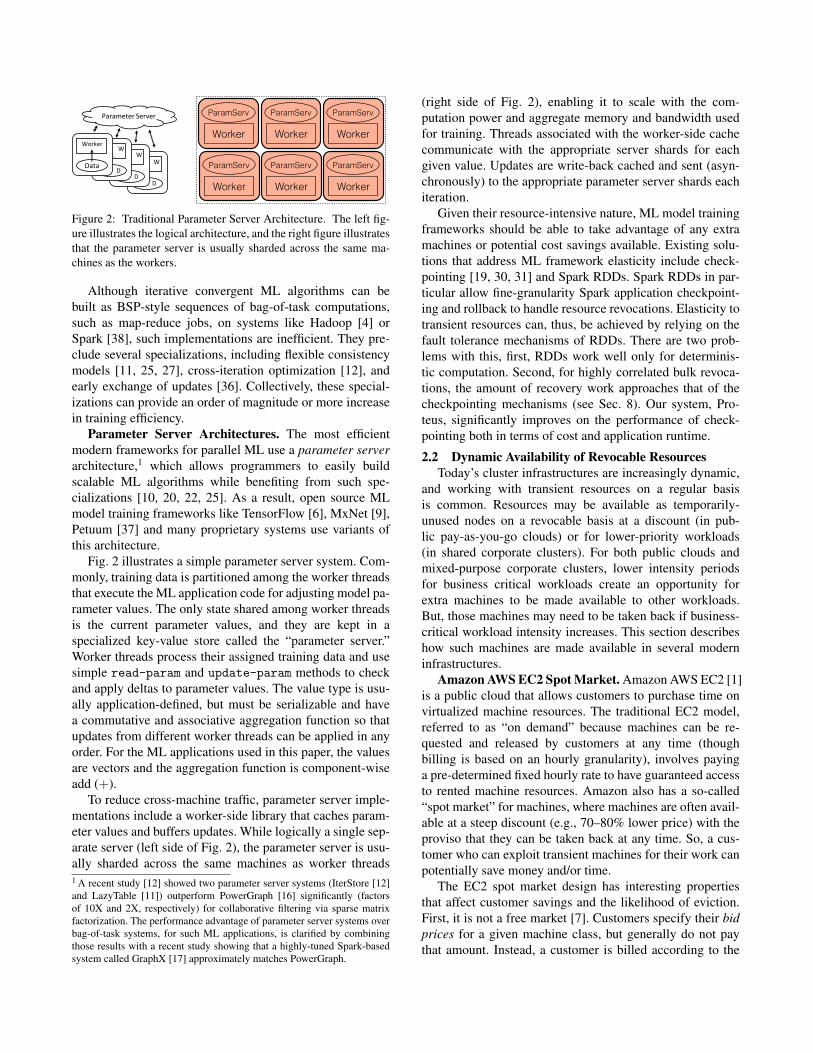
Figure 2: Traditional Parameter Server Architecture. The left fig-ure illustrates the logical architecture, and the right figure illustratesthat the parameter server is usually sharded across the same ma-chines as the workers.

Although iterative convergent ML algorithms can bebuilt as BSP-style sequences of bag-of-task computations,such as map-reduce jobs, on systems like Hadoop [4] orSpark [38], such implementations are inefficient. They pre-clude several specializations, including flexible consistencymodels [11, 25, 27], cross-iteration optimization [12], andearly exchange of updates [36]. Collectively, these special-izations can provide an order of magnitude or more increasein training efficiency.

Parameter Server Architectures. The most efficientmodern frameworks for parallel ML use a parameter serverarchitecture,1 which allows programmers to easily buildscalable ML algorithms while benefiting from such spe-cializations [10, 20, 22, 25]. As a result, open source MLmodel training frameworks like TensorFlow [6], MxNet [9],Petuum [37] and many proprietary systems use variants ofthis architecture.

Fig. 2 illustrates a simple parameter server system. Com-monly, training data is partitioned among the worker threadsthat execute the ML application code for adjusting model pa-rameter values. The only state shared among worker threadsis the current parameter values, and they are kept in aspecialized key-value store called the “parameter server.”Worker threads process their assigned training data and usesimple read-param and update-param methods to checkand apply deltas to parameter values. The value type is usu-ally application-defined, but must be serializable and havea commutative and associative aggregation function so thatupdates from different worker threads can be applied in anyorder. For the ML applications used in this paper, the valuesare vectors and the aggregation function is component-wiseadd (+).

To reduce cross-machine traffic, parameter server imple-mentations include a worker-side library that caches param-eter values and buffers updates. While logically a single sep-arate server (left side of Fig. 2), the parameter server is usu-ally sharded across the same machines as worker threads1 A recent study [12] showed two parameter server systems (IterStore [12]and LazyTable [11]) outperform PowerGraph [16] significantly (factorsof 10X and 2X, respectively) for collaborative filtering via sparse matrixfactorization. The performance advantage of parameter server systems overbag-of-task systems, for such ML applications, is clarified by combiningthose results with a recent study showing that a highly-tuned Spark-basedsystem called GraphX [17] approximately matches PowerGraph.

(right side of Fig. 2), enabling it to scale with the com-putation power and aggregate memory and bandwidth usedfor training. Threads associated with the worker-side cachecommunicate with the appropriate server shards for eachgiven value. Updates are write-back cached and sent (asyn-chronously) to the appropriate parameter server shards eachiteration.

Given their resource-intensive nature, ML model trainingframeworks should be able to take advantage of any extramachines or potential cost savings available. Existing solu-tions that address ML framework elasticity include check-pointing [19, 30, 31] and Spark RDDs. Spark RDDs in par-ticular allow fine-granularity Spark application checkpoint-ing and rollback to handle resource revocations. Elasticity totransient resources can, thus, be achieved by relying on thefault tolerance mechanisms of RDDs. There are two prob-lems with this, first, RDDs work well only for determinis-tic computation. Second, for highly correlated bulk revoca-tions, the amount of recovery work approaches that of thecheckpointing mechanisms (see Sec. 8). Our system, Pro-teus, significantly improves on the performance of check-pointing both in terms of cost and application runtime.

2.2 Dynamic Availability of Revocable ResourcesToday’s cluster infrastructures are increasingly dynamic,

and working with transient resources on a regular basisis common. Resources may be available as temporarily-unused nodes on a revocable basis at a discount (in pub-lic pay-as-you-go clouds) or for lower-priority workloads(in shared corporate clusters). For both public clouds andmixed-purpose corporate clusters, lower intensity periodsfor business critical workloads create an opportunity forextra machines to be made available to other workloads.But, those machines may need to be taken back if business-critical workload intensity increases. This section describeshow such machines are made available in several moderninfrastructures.

Amazon AWS EC2 Spot Market. Amazon AWS EC2 [1]is a public cloud that allows customers to purchase time onvirtualized machine resources. The traditional EC2 model,referred to as “on demand” because machines can be re-quested and released by customers at any time (thoughbilling is based on an hourly granularity), involves payinga pre-determined fixed hourly rate to have guaranteed accessto rented machine resources. Amazon also has a so-called“spot market” for machines, where machines are often avail-able at a steep discount (e.g., 70–80% lower price) with theproviso that they can be taken back at any time. So, a cus-tomer who can exploit transient machines for their work canpotentially save money and/or time.

The EC2 spot market design has interesting propertiesthat affect customer savings and the likelihood of eviction.First, it is not a free market [7]. Customers specify their bidprices for a given machine class, but generally do not paythat amount. Instead, a customer is billed according to the

Jan 19 Jan 20 Jan 21 Jan 22 Jan 23 Jan 240

1

2

3

4

5

Date

Price

per

Hou

r ($)

c4.2xlargec4.xlargeOn−Demand

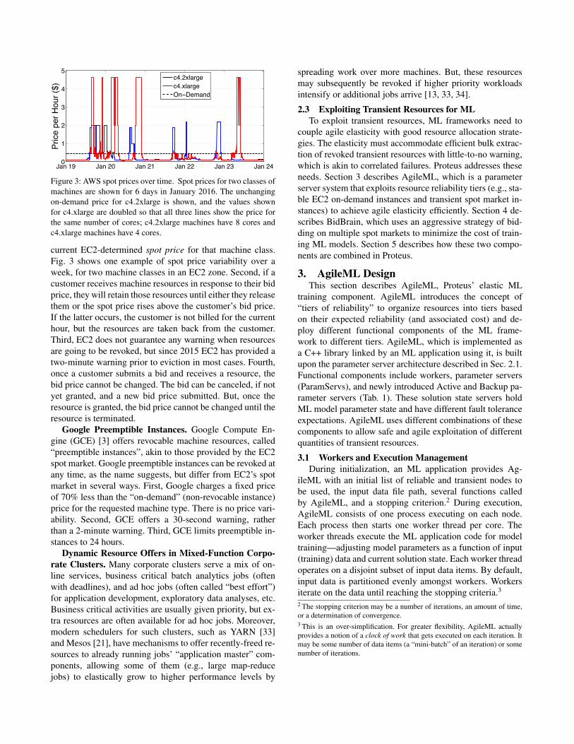
Figure 3: AWS spot prices over time. Spot prices for two classes ofmachines are shown for 6 days in January 2016. The unchangingon-demand price for c4.2xlarge is shown, and the values shownfor c4.xlarge are doubled so that all three lines show the price forthe same number of cores; c4.2xlarge machines have 8 cores andc4.xlarge machines have 4 cores.

current EC2-determined spot price for that machine class.Fig. 3 shows one example of spot price variability over aweek, for two machine classes in an EC2 zone. Second, if acustomer receives machine resources in response to their bidprice, they will retain those resources until either they releasethem or the spot price rises above the customer’s bid price.If the latter occurs, the customer is not billed for the currenthour, but the resources are taken back from the customer.Third, EC2 does not guarantee any warning when resourcesare going to be revoked, but since 2015 EC2 has provided atwo-minute warning prior to eviction in most cases. Fourth,once a customer submits a bid and receives a resource, thebid price cannot be changed. The bid can be canceled, if notyet granted, and a new bid price submitted. But, once theresource is granted, the bid price cannot be changed until theresource is terminated.

Google Preemptible Instances. Google Compute En-gine (GCE) [3] offers revocable machine resources, called“preemptible instances”, akin to those provided by the EC2spot market. Google preemptible instances can be revoked atany time, as the name suggests, but differ from EC2’s spotmarket in several ways. First, Google charges a fixed priceof 70% less than the “on-demand” (non-revocable instance)price for the requested machine type. There is no price vari-ability. Second, GCE offers a 30-second warning, ratherthan a 2-minute warning. Third, GCE limits preemptible in-stances to 24 hours.

Dynamic Resource Offers in Mixed-Function Corpo-rate Clusters. Many corporate clusters serve a mix of on-line services, business critical batch analytics jobs (oftenwith deadlines), and ad hoc jobs (often called “best effort”)for application development, exploratory data analyses, etc.Business critical activities are usually given priority, but ex-tra resources are often available for ad hoc jobs. Moreover,modern schedulers for such clusters, such as YARN [33]and Mesos [21], have mechanisms to offer recently-freed re-sources to already running jobs’ “application master” com-ponents, allowing some of them (e.g., large map-reducejobs) to elastically grow to higher performance levels by

spreading work over more machines. But, these resourcesmay subsequently be revoked if higher priority workloadsintensify or additional jobs arrive [13, 33, 34].

2.3 Exploiting Transient Resources for MLTo exploit transient resources, ML frameworks need to

couple agile elasticity with good resource allocation strate-gies. The elasticity must accommodate efficient bulk extrac-tion of revoked transient resources with little-to-no warning,which is akin to correlated failures. Proteus addresses theseneeds. Section 3 describes AgileML, which is a parameterserver system that exploits resource reliability tiers (e.g., sta-ble EC2 on-demand instances and transient spot market in-stances) to achieve agile elasticity efficiently. Section 4 de-scribes BidBrain, which uses an aggressive strategy of bid-ding on multiple spot markets to minimize the cost of train-ing ML models. Section 5 describes how these two compo-nents are combined in Proteus.

3. AgileML DesignThis section describes AgileML, Proteus’ elastic ML

training component. AgileML introduces the concept of“tiers of reliability” to organize resources into tiers basedon their expected reliability (and associated cost) and de-ploy different functional components of the ML frame-work to different tiers. AgileML, which is implemented asa C++ library linked by an ML application using it, is builtupon the parameter server architecture described in Sec. 2.1.Functional components include workers, parameter servers(ParamServs), and newly introduced Active and Backup pa-rameter servers (Tab. 1). These solution state servers holdML model parameter state and have different fault toleranceexpectations. AgileML uses different combinations of thesecomponents to allow safe and agile exploitation of differentquantities of transient resources.

3.1 Workers and Execution ManagementDuring initialization, an ML application provides Ag-

ileML with an initial list of reliable and transient nodes tobe used, the input data file path, several functions calledby AgileML, and a stopping criterion.2 During execution,AgileML consists of one process executing on each node.Each process then starts one worker thread per core. Theworker threads execute the ML application code for modeltraining—adjusting model parameters as a function of input(training) data and current solution state. Each worker threadoperates on a disjoint subset of input data items. By default,input data is partitioned evenly amongst workers. Workersiterate on the data until reaching the stopping criteria.3

2 The stopping criterion may be a number of iterations, an amount of time,or a determination of convergence.3 This is an over-simplification. For greater flexibility, AgileML actuallyprovides a notion of a clock of work that gets executed on each iteration. Itmay be some number of data items (a “mini-batch” of an iteration) or somenumber of iterations.

WorkerWorker

Spot Instances (Cheap)

Elasticity Controller

Worker Worker Worker

Worker

Worker

On-Demand Instances (Reliable)

ParamServe

Worker

ParamServe

(a) Stage 1

Worker

Worker

Spot Instances (Cheap)

On-Demand Instances (Reliable)

Elasticity Controller

Worker

ActivePS

Worker

Worker

ActivePS

Worker

Worker

ActivePS

BackupPS

Worker

BackupPS

(b) Stage 2Spot Instances (Cheap)

On-Demand Instances (Reliable)Elasticity Controller BackupPS

ActivePS

WorkerActivePS

WorkerActivePS

WorkerActivePS

WorkerActivePS

Worker

ActivePS

WorkerActivePS

WorkerActivePS

WorkerActivePS

WorkerActivePS

Worker

Worker Worker Worker Worker Worker

Worker Worker Worker Worker Worker

(c) Stage 3

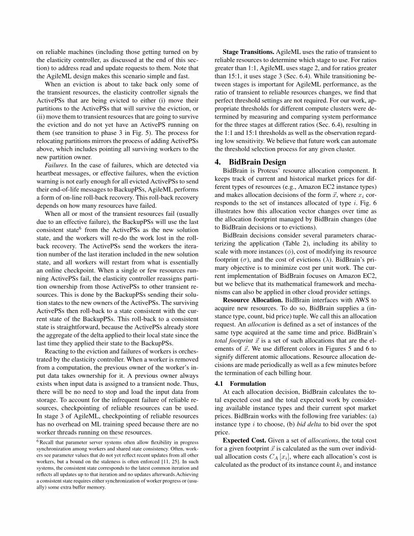
Figure 4: Three stages of AgileML architecture. Stage 1: ParamServs only on reliable machine. Stage 2: ActivePSs on transient andBackupPSs on reliable. Stage 3: No Workers on Reliable Machines.

3.2 ArchitectureThis section describes how AgileML uses reliability tiers

and the mechanism of moving between its different stagesof execution. At a high level, AgileML enables ML appli-cations to run on a dynamic mix of reliable and transientmachines, maintaining the state required for continued oper-ation on reliable machines, while taking advantage of tran-sient machine availability. AgileML uses three stages of sys-tem functionality partitioning in order to avoid bottleneck-ing the reliable nodes, as the ratio of transient to reliableresources grows.

Stage 1: Parameter Servers Only on Reliable Ma-chines. For most ML applications including K-means, DNN,Logistic Regression, Sparse Coding, as well as MF, MLR,and LDA (Sec. 6.2), the workers are stateless, while theParamServs contain the current solution state. AgileML’sfirst stage spreads the parameter server across reliable ma-chines only, using transient nodes only for workers, therebytaking advantage of these two primary levels of machine re-liability. This has the effect of removing all solution statefrom transient machines. Fig. 4a illustrates a running ex-ample of eight AWS EC2 machines with six spot instances(transient) and two on-demand instances (reliable).

Pros: By removing parameter state from transient re-sources, AgileML is able to utilize them without losingprogress when transient resources are revoked (or fail). Un-like a traditional parameter-server architecture, no check-

ParamServs Serve solution state for workers and al-ways run on reliable resources

BackupPSs Serve as a hot backup for solution stateserved by ActivePSs and always runs onreliable resources

ActivePSs Serve solution state for workers, pe-riodically pushing aggregated updatesto BackupPSs, and run on transient re-sources

Table 1: Types of solution state servers used by AgileML

pointing is required to assist with using transient resources.4

Cons: While stage 1 successfully removes state from tran-sient resources, it causes a network bottleneck (Sec. 6.4)when the ratio of transient to reliable resources grows toolarge. With 60 transient and 4 reliable machines, for ex-ample, the network bottleneck to the ParamServs slows theMF application by over 85%. Limiting this ratio is unde-sirable, as it caps achievable savings/benefits from transientresources.

Stage 2: ActivePSs on Transient Machines and Back-upPSs on Reliable Machines. For higher transient to reli-able node ratio, AgileML switches to stage 2 (Fig. 4b). Stage2 uses a primary-backup model for parameter servers, usingtransient nodes for an active server (ActivePS) and reliablenodes for the hot standby (BackupPS). This shifts the heavynetwork load from the few reliable resources to the manytransient resources. Solution state is sharded across the setof ActivePS instances. Workers send all updates and read re-quests to the ActivePSs, which update their state and pushupdates in bulk to the BackupPSs. Solution state affected bytransient node failures or evictions is recovered from Back-upPSs. Stage 2 improves on stage 1 for higher transient-to-reliable ratios (Sec. 6.4) but loses to an all-reliable baselineby 2x for ratios exceeding 63:1.

Stage 3: No Workers on Reliable Machines. Workerscolocated with BackupPSs on reliable machines were foundto cause straggler effects at transient-to-reliable ratios be-yond 15:1, causing Proteus’ performance drop relative to thePS baseline. Stage 3 simply removes these workers (Fig. 4c),allowing AgileML to match all-reliable performance levels(Sec. 6.4). The optimal ratio threshold to switch to stage 3depends on the network bandwidth, transient-to-reliable ra-tio and the size of the model.

Transitioning Between Stages. AgileML dynamicallytransitions between these stages to match the number of tran-sient nodes available. Transitioning between stages 1 and 2involves switching between a set of ParamServs and the ac-tive/backup PS pair. This process is described in Sec. 3.3.4 In AgileML, there is benefit in checkpointing the reliable resources in casethey fail, however as we show later in this section, this checkpointing hasno overhead on system performance in stages 2 and 3.

BackupPSMachine 0

ActivePSstate part1

Input 1-10

Machine 1

Input 11-20ActivePS

state part2

Input 21-30

Machine 2

Input 31-40

BackupPSMachine 0

ActivePSstate part1

Input 1-10

Machine 1

ActivePSstate part2

Input 11-20

Machine 2

Machine 3

Input 21-30

Machine 4Input 31-40

BackupPSMachine 0

ActivePSstate part1

Input 1-10

Machine 3

Input 11-20ActivePS

state part2

Input 21-30

Machine 4

Input 31-40

Add 2 more spot instances 2 instances evicted

Figure 5: AgileML component and data transitions as resources are added and evicted. In this toy example, there are 40 pieces of input data.Initially, one on-demand Machine 0 runs BackupPS, and 2 spot instances (Machine 1,2) are processing 1

2of the input data each. 2 new spot

instances (Machine 3,4) are added, at the same time, price, of the same type, and shown in the same color (we refer to these atomic sets asallocations, described in Sec. 4). Each new instance ∈ {3, 4} loads 1

2of the input data, but works only on 1

4of it. An eviction of the 2 yellow

spot instances triggers the second transition. The remaining spot instances assume ownership of the evicted input data with minimal delay.

When scaling up, workers are directed to send their requeststo ActivePSs started in the background. When scaling down,ActivePSs push their updates to BackupPSs, which becomeParamServs. The worker requests are then redirected to theParamServs. This transition is done with minimal overheadin the background. Transitioning between stages 2 and 3boils down to re-assigning work between reliable and tran-sient resources. Scaling up, work is offloaded from workerson reliable nodes to workers on transient nodes, followedby shutting down the former workers. Transitioning back tostage 2 requires reassigning input data to reliable workers.This change of assignment incurs zero run-time overhead,as it involves just a single worker notification message.5

Elasticity Controller: This component of AgileML makesdecisions to switch between stages based on the transient-to-reliable ratio and the network bandwidth. It is responsiblefor (a) tracking which resources are participating in ongoingcomputations, (b) assigning a subset of input data to eachworker, and (c) starting new ActivePSs. On eviction, it re-shards the solution state and shuts down ActivePSs usingpolicies discussed next.

3.3 Handling Elasticity: Policy and MechanismThe toy example in Fig. 5 illustrates how AgileML han-

dles adding and removing resources from an ongoing com-putation. We evaluate AgileML’s effectiveness at handlingsuch elasticity in Section 6.6.

Scaling Up. Workers. Once a node becomes available,and the appropriate software has been initialized, it contactsthe elasticity controller responsible for the job and receivesits input data assignment (see transition to phase 2 in Fig. 5).It loads the data (from S3 storage for AWS EC2) and sig-nals the elasticity controller that it’s ready. The elasticitycontroller then signals corresponding workers to update theirworking sets. ActivePS. AgileML achieves best performancewhen running ActivePSs on half of the resources (Sec. 6.4).This ratio is thus maintained when scaling the resource foot-print. When the resource footprint increases, AgileML starts5 Input data assigned to workers on reliable resources is preloaded byworkers on transient resources, simplifying the transition from stage 2 to 3.

new ActivePSs on the longest running transient resourcesthat do not yet have an ActivePS. It notifies the resource tohost the ActivePS and serve a given partition assignment. Apartition is a unique subset of the parameter state. Duringstart-up, AgileML divides the parameter state into N parti-tions, where N is the maximum number of ActivePSs thatcan exist at any one point. We found that setting N equalto half of the maximum number of resources that could beused by AgileML at any point to be effective. Each parti-tion is assigned to a ParamServ. In stage 2 and 3 each parti-tion is also assigned to an ActivePS, which is responsible forforwarding updates applied to the partition to the BackupPSthat owns it. By using partitions in this way, AgileML avoidsthe need to re-shard the parameter state when adding or re-moving servers, instead re-assigning partitions as needed.

The resource that starts the new ActivePS contacts theprevious partition owner for a copy of the partition. The orig-inal owner points all workers to the new partition owner.During ownership propagation, all partition messages areforwarded to the new ActivePS. Workers and ActivePS ad-ditions happen in the background with negligible impact onsystem performance (Sec. 6.6).

Scaling Down. AgileML differentiates between evictionsand failures based on whether it received a warning, andit handles them differently. When resources are removedfrom an ongoing computation after some warning, such asthe two-minute warning offered by AWS or the 30-secondwarning offered by GCE, we call this an eviction. Whenresources are removed without warning or with a warningdetected with insufficient lead time, we call this a failure oran effective failure, respectively.

Evictions. AgileML’s elasticity controller checks for evic-tion warnings every 5s. These warnings consist of a set ofinstances marked for eviction, if any. When this set includesall transient resources, the elasticity controller signals allActivePSs to push their most recent consistent state to theBackupPSs and cease operation. A special end-of-life flag isappended to these updates to signal the last message fromActivePS to BackupPS. When the BackupPSs receive end-of-life messages from ActivePSs, they signal any workers

on reliable machines (including those getting turned on bythe elasticity controller, as discussed at the end of this sec-tion) to address read and update requests to them. Note thatthe AgileML design makes this scenario simple and fast.

When an eviction is about to take back only some ofthe transient resources, the elasticity controller signals theActivePSs that are being evicted to either (i) move theirpartitions to the ActivePSs that will survive the eviction, or(ii) move them to transient resources that are going to survivethe eviction and do not yet have an ActivePS running onthem (see transition to phase 3 in Fig. 5). The process forrelocating partitions mirrors the process of adding ActivePSsabove, which includes pointing all surviving workers to thenew partition owner.

Failures. In the case of failures, which are detected viaheartbeat messages, or effective failures, when the evictionwarning is not early enough for all evicted ActivePSs to sendtheir end-of-life messages to BackupPSs, AgileML performsa form of on-line roll-back recovery. This roll-back recoverydepends on how many resources have failed.

When all or most of the transient resources fail (usuallydue to an effective failure), the BackupPSs will use the lastconsistent state6 from the ActivePSs as the new solutionstate, and the workers will re-do the work lost in the roll-back recovery. The ActivePSs send the workers the itera-tion number of the last iteration included in the new solutionstate, and all workers will restart from what is essentiallyan online checkpoint. When a single or few resources run-ning ActivePSs fail, the elasticity controller reassigns parti-tion ownership from those ActivePSs to other transient re-sources. This is done by the BackupPSs sending their solu-tion states to the new owners of the ActivePSs. The survivingActivePSs then roll-back to a state consistent with the cur-rent state of the BackupPSs. This roll-back to a consistentstate is straightforward, because the ActivePSs already storethe aggregate of the delta applied to their local state since thelast time they applied their state to the BackupPSs.

Reacting to the eviction and failures of workers is orches-trated by the elasticity controller. When a worker is removedfrom a computation, the previous owner of the worker’s in-put data takes ownership for it. A previous owner alwaysexists when input data is assigned to a transient node. Thus,there will be no need to stop and load the input data fromstorage. To account for the infrequent failure of reliable re-sources, checkpointing of reliable resources can be used.In stage 3 of AgileML, checkpointing of reliable resourceshas no overhead on ML training speed because there are noworker threads running on these resources.6 Recall that parameter server systems often allow flexibility in progresssynchronization among workers and shared state consistency. Often, work-ers see parameter values that do not yet reflect recent updates from all otherworkers, but a bound on the staleness is often enforced [11, 25]. In suchsystems, the consistent state corresponds to the latest common iteration andreflects all updates up to that iteration and no updates afterwards.Achievinga consistent state requires either synchronization of worker progress or (usu-ally) some extra buffer memory.

Stage Transitions. AgileML uses the ratio of transient toreliable resources to determine which stage to use. For ratiosgreater than 1:1, AgileML uses stage 2, and for ratios greaterthan 15:1, it uses stage 3 (Sec. 6.4). While transitioning be-tween stages is important for AgileML performance, as theratio of transient to reliable resources changes, we find thatperfect threshold settings are not required. For our work, ap-propriate thresholds for different compute clusters were de-termined by measuring and comparing system performancefor the three stages at different ratios (Sec. 6.4), resulting inthe 1:1 and 15:1 thresholds as well as the observation regard-ing low sensitivity. We believe that future work can automatethe threshold selection process for any given cluster.

4. BidBrain DesignBidBrain is Proteus’ resource allocation component. It

keeps track of current and historical market prices for dif-ferent types of resources (e.g., Amazon EC2 instance types)and makes allocation decisions of the form ~x, where xi cor-responds to the set of instances allocated of type i. Fig. 6illustrates how this allocation vector changes over time asthe allocation footprint managed by BidBrain changes (dueto BidBrain decisions or to evictions).

BidBrain decisions consider several parameters charac-terizing the application (Table 2), including its ability toscale with more instances (φ), cost of modifying its resourcefootprint (σ), and the cost of evictions (λ). BidBrain’s pri-mary objective is to minimize cost per unit work. The cur-rent implementation of BidBrain focuses on Amazon EC2,but we believe that its mathematical framework and mecha-nisms can also be applied in other cloud provider settings.

Resource Allocation. BidBrain interfaces with AWS toacquire new resources. To do so, BidBrain supplies a (in-stance type, count, bid price) tuple. We call this an allocationrequest. An allocation is defined as a set of instances of thesame type acquired at the same time and price. BidBrain’stotal footprint ~x is a set of such allocations that are the el-ements of ~x. We use different colors in Figures 5 and 6 tosignify different atomic allocations. Resource allocation de-cisions are made periodically as well as a few minutes beforethe termination of each billing hour.

4.1 FormulationAt each allocation decision, BidBrain calculates the to-

tal expected cost and the total expected work by consider-ing available instance types and their current spot marketprices. BidBrain works with the following free variables: (a)instance type i to choose, (b) bid delta to bid over the spotprice.

Expected Cost. Given a set of allocations, the total costfor a given footprint ~x is calculated as the sum over individ-ual allocation costs CA [xi], where each allocation’s cost iscalculated as the product of its instance count ki and instance

[0]-(k=1,c4.xlarge,$0.2,W=0)

[1]-(k=2,m4.xlarge,$0.1,W=2)

[0]-(k=1,c4.xlarge,$0.2,W=0)[1]-(k=2,m4.xlarge,$0.1,W=2)[2]-(k=2,c4.xlarge,$0.05,W=2)

[2]-(k=2,c4.xlarge,$0.05,W=2)

Add 2 Spot Instances 2 Instances Evicted

Exp.

Cos

t/(To

tal w

ork

in p

hase

)

Phase 1 Phase 2 Phase 3

[0]-(k=1,c4.xlarge,$0.2,W=0)

Exp Total: Cost: $0.3, Work: 2

Exp Total: Cost:$0.35, Work: 4

Exp Total: Cost:$0.25, Work: 2

On-DemandOn-Demand

On-Demand

Figure 6: Expected cost per unit work for the toy example transitions in Fig. 5. Each block represents an allocation (Sec. 4), described byhow many instances are in the allocation (k), instance type, the expected cost of the allocation, and the expected work produced by thisallocation. Each block’s height equates to that allocation’s relative contribution to the cost of the total work done in its phase. Combiningthe blocks’ heights in each phase equates to the total expected cost per unit work for that phase. In phase 1, BidBrain has an expensive,required on-demand allocation (red) that produces no work and a spot allocation (yellow). The on-demand instance type is pre-determined tobe c4.xlarge and is never terminated by BidBrain, even if it negatively affects cost-per-work. In phase 2, BidBrain further amortizes the costof the red allocation by adding a second spot allocation [2] (green), which lowers the total expected cost-per-work. This transition increasesits actual cost at that moment, but reduces the final cost by decreasing the amount of time for which the on-demand allocation is needed.

price Pi:

CA =

n∑i=0

CA[xi] =

n∑i=0

ki ∗ Pi

One of BidBrain’s features is to reason about the probabil-ity of free compute it can get if its instances are evictedbefore the billing hour expires. If the allocation is evicted,AWS refunds the amount charged at the beginning of thecurrent billing hour. To capture this, BidBrain calculates theexpected cost of an allocation by considering the probabilityof eviction βi for a given instance type i at a given bid delta.There are only two possibilities: an allocation can either beevicted (with probability βi) or it will reach the end of itsbilling hour in the remaining tr minutes (with probability1 − βi). The expected cost can, therefore, be written downby the definition of expectation (Eq. 1).

CA[xi] = (1− βi) ∗ Pi ∗ ki ∗ tr + βi ∗ 0 ∗ ki ∗ tr (1)

Estimating Evictions. To estimate βi in Eq. 1, BidBrainuses historical AWS spot market price data. This histori-cal data is gathered individually for each instance type ineach availability zone and indicates the price at each instantin time. Combining such data with knowledge that spot in-stances are evicted when the price rises above the bid, Bid-Brain computes the historical probability of being evictedwithin the hour and the median time to eviction for a given

β Probability that allocation is evicted (0-1)φ How efficiently application scales (0-1)σ Overhead of adding/removing resources (min)λ Overhead of evicting resource (min)ν Work produced by instance typeωi Max compute time remaining in allocation i

CA Expected cost of a set of allocations ($)WA Expected work of a set of allocationsEA Expected cost per work of a set of allocations

Table 2: Summary of parameters used by BidBrain

bid delta. The bid delta is the difference between the bidprice and the market price. Using the AWS spot market tracefrom March to June of 2016, we ran simulations with a widerange of bid deltas [$0.00001,$0.4] and recorded the proba-bility of getting evicted within the hour, β, and the mediantime to eviction. Using this information, BidBrain estimatesthe probability of eviction for any allocation.

Expected Work. BidBrain explicitly reasons about theexpected amount of work each allocation is expected toproduce. To capture this, BidBrain computes the expecteduseful compute time ∆ti for each allocation by consideringfactors such as eviction overhead, overhead for resourceaddition, and scalability of the application.

The maximum useful compute time of any allocation isthe time remaining in the current billing hour ωi. If Bid-Brain expects the allocation to be evicted prior to the endof the billing hour, it reduces ωi accordingly. The evictionof any allocation reduces the useful compute of each allo-cation xi by the eviction overhead λ of the application. Theprobability of an eviction for a set of allocations is computedas: 1 −

∏nj=0(1 − βj), where βj is the probability of evic-

tion for allocation j. When considering removing or addingresources, BidBrain subtracts this overhead σ from the ex-pected compute time for each allocation (Eq. 2).

The expected work for an allocation is the product ofits resources ki, expected useful compute time ∆ti and thework produced per time by that instance type ν.7 BidBrainexpresses the expected work for a set of allocations as thesum of each allocation’s expected work reduced by the scal-ability overhead φ of the application (Eq. 3).

∆ti = ωi − (1−n∏

j=0

(1− βj)) ∗ λ− σ (2)

WA = (

n∑i=0

ki ∗∆ti ∗ ν) ∗ φ (3)

7 For ML workloads performed by AgileML, work produced is propor-tional to the number of cores on an instance. For example, ν of a c4.2xlargeinstance (8 cores) is equivalent to 2 * ν of a c4.xlarge instance (4 cores).

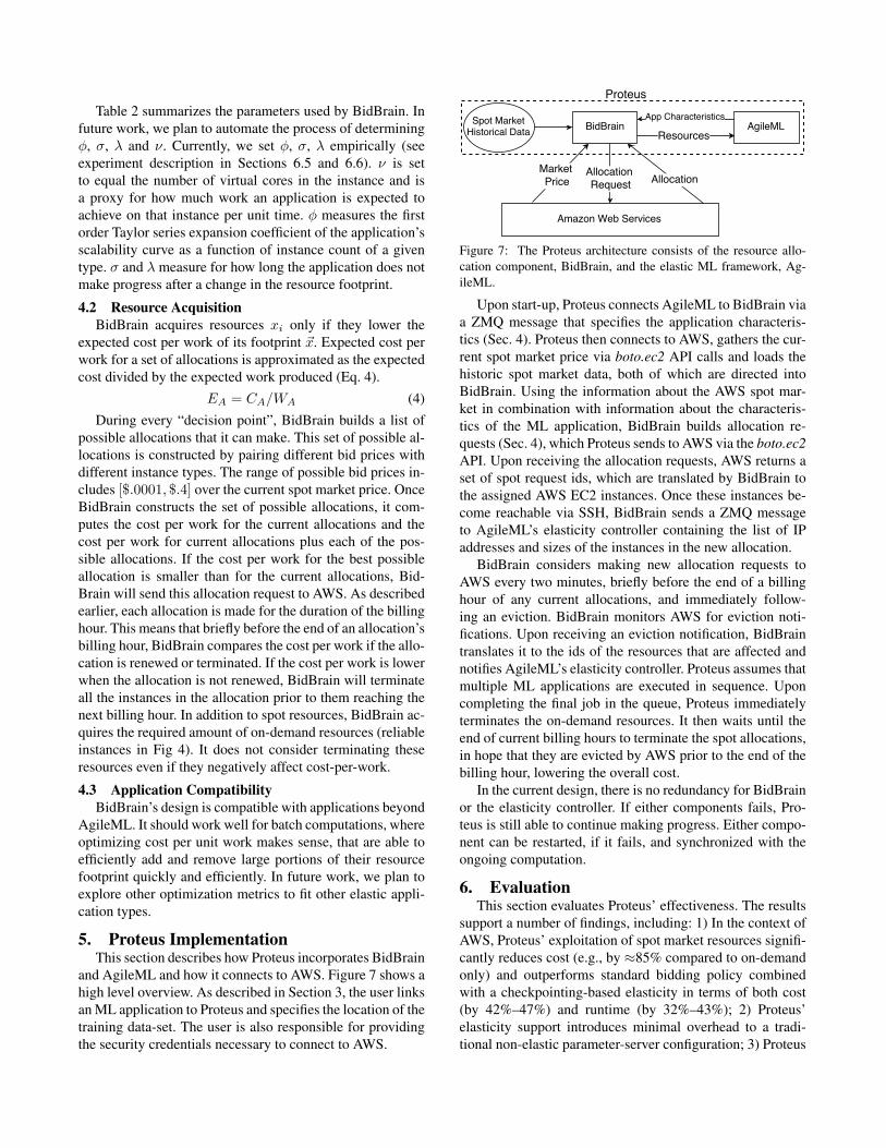
Table 2 summarizes the parameters used by BidBrain. Infuture work, we plan to automate the process of determiningφ, σ, λ and ν. Currently, we set φ, σ, λ empirically (seeexperiment description in Sections 6.5 and 6.6). ν is setto equal the number of virtual cores in the instance and isa proxy for how much work an application is expected toachieve on that instance per unit time. φ measures the firstorder Taylor series expansion coefficient of the application’sscalability curve as a function of instance count of a giventype. σ and λ measure for how long the application does notmake progress after a change in the resource footprint.

4.2 Resource AcquisitionBidBrain acquires resources xi only if they lower the

expected cost per work of its footprint ~x. Expected cost perwork for a set of allocations is approximated as the expectedcost divided by the expected work produced (Eq. 4).

EA = CA/WA (4)During every “decision point”, BidBrain builds a list of

possible allocations that it can make. This set of possible al-locations is constructed by pairing different bid prices withdifferent instance types. The range of possible bid prices in-cludes [$.0001, $.4] over the current spot market price. OnceBidBrain constructs the set of possible allocations, it com-putes the cost per work for the current allocations and thecost per work for current allocations plus each of the pos-sible allocations. If the cost per work for the best possibleallocation is smaller than for the current allocations, Bid-Brain will send this allocation request to AWS. As describedearlier, each allocation is made for the duration of the billinghour. This means that briefly before the end of an allocation’sbilling hour, BidBrain compares the cost per work if the allo-cation is renewed or terminated. If the cost per work is lowerwhen the allocation is not renewed, BidBrain will terminateall the instances in the allocation prior to them reaching thenext billing hour. In addition to spot resources, BidBrain ac-quires the required amount of on-demand resources (reliableinstances in Fig 4). It does not consider terminating theseresources even if they negatively affect cost-per-work.

4.3 Application CompatibilityBidBrain’s design is compatible with applications beyond

AgileML. It should work well for batch computations, whereoptimizing cost per unit work makes sense, that are able toefficiently add and remove large portions of their resourcefootprint quickly and efficiently. In future work, we plan toexplore other optimization metrics to fit other elastic appli-cation types.

5. Proteus ImplementationThis section describes how Proteus incorporates BidBrain

and AgileML and how it connects to AWS. Figure 7 shows ahigh level overview. As described in Section 3, the user linksan ML application to Proteus and specifies the location of thetraining data-set. The user is also responsible for providingthe security credentials necessary to connect to AWS.

Figure 7: The Proteus architecture consists of the resource allo-cation component, BidBrain, and the elastic ML framework, Ag-ileML.

Upon start-up, Proteus connects AgileML to BidBrain viaa ZMQ message that specifies the application characteris-tics (Sec. 4). Proteus then connects to AWS, gathers the cur-rent spot market price via boto.ec2 API calls and loads thehistoric spot market data, both of which are directed intoBidBrain. Using the information about the AWS spot mar-ket in combination with information about the characteris-tics of the ML application, BidBrain builds allocation re-quests (Sec. 4), which Proteus sends to AWS via the boto.ec2API. Upon receiving the allocation requests, AWS returns aset of spot request ids, which are translated by BidBrain tothe assigned AWS EC2 instances. Once these instances be-come reachable via SSH, BidBrain sends a ZMQ messageto AgileML’s elasticity controller containing the list of IPaddresses and sizes of the instances in the new allocation.

BidBrain considers making new allocation requests toAWS every two minutes, briefly before the end of a billinghour of any current allocations, and immediately follow-ing an eviction. BidBrain monitors AWS for eviction noti-fications. Upon receiving an eviction notification, BidBraintranslates it to the ids of the resources that are affected andnotifies AgileML’s elasticity controller. Proteus assumes thatmultiple ML applications are executed in sequence. Uponcompleting the final job in the queue, Proteus immediatelyterminates the on-demand resources. It then waits until theend of current billing hours to terminate the spot allocations,in hope that they are evicted by AWS prior to the end of thebilling hour, lowering the overall cost.

In the current design, there is no redundancy for BidBrainor the elasticity controller. If either components fails, Pro-teus is still able to continue making progress. Either compo-nent can be restarted, if it fails, and synchronized with theongoing computation.

6. EvaluationThis section evaluates Proteus’ effectiveness. The results

support a number of findings, including: 1) In the context ofAWS, Proteus’ exploitation of spot market resources signifi-cantly reduces cost (e.g., by ≈85% compared to on-demandonly) and outperforms standard bidding policy combinedwith a checkpointing-based elasticity in terms of both cost(by 42%–47%) and runtime (by 32%–43%); 2) Proteus’elasticity support introduces minimal overhead to a tradi-tional non-elastic parameter-server configuration; 3) Proteus

enacts bulk machine additions and revocations with minimaldisruption, performing most setup actions in the background.

6.1 Experimental SetupExperimental Platforms. We report results for experi-

ments on two virtual cluster configurations on AWS. Cluster-A is a cluster of 64 Amazon EC2 c4.2xlarge instances. Eachinstance has 8 vCPUs and 15 GB memory, running 64-bitUbuntu Server 14.04 LTS (HVM). Cluster-B is a cluster of128 Amazon EC2 c4.xlarge instances. Each instance has 4vCPUs and 7.5 GB memory, running 64-bit Ubuntu Server14.04 LTS (HVM). From our testing using iperf, we ob-serve a bandwidth of 1 Gbps between each pair of EC2instances.

6.2 Application BenchmarksWe use three popular iterative ML applications.Matrix Factorization (MF) is a technique (a.k.a. col-

laborative filtering) commonly used in recommendation sys-tems, such as recommending movies to users on Netflix. Thegoal is to discover latent interactions between the two enti-ties (e.g., users and movies). Given a partially filled matrixX (e.g., a matrix where entry (i, j) is user i’s rating of moviej), MF factorizes X into factor matrices L and R such thattheir product approximates X (i.e., X ≈ LR). Like oth-ers [11, 14, 24], our MF implementation uses the stochasticgradient descent (SGD) algorithm. Each worker is assigned asubset of the observed entries in X; in every iteration, eachworker processes every element of its assigned subset andupdates the corresponding row of L and column of R basedon the gradient. L and R are stored in the parameter server.

Our MF experiments use the Netflix dataset, which is a480k-by-18k sparse matrix with 100m known elements, andfactor it into two matrices with rank 1000. We also use asynthetically enlarged version of the Netflix dataset that is256 times the original. It is a 7683k-by-284k sparse matrixwith 4.24 billion known elements with rank 100.

Multinomial Logistic Regression (MLR) is a popu-lar model for multi-way classification, often used in thelast layer of deep learning models for image classifica-tion [23] or text classification [26]. In MLR, the likelihoodthat each (d-dimensional) observation x ∈ Rd belongs toeach of the K classes is modeled by softmax transformationp(class=k|x) =

exp(wTk x)∑

j exp(wTj x)

, where {wj}Kj=1 are the linear(d-dimensional) weights associated with each class and areconsidered the model parameters. The weight vectors arestored in the parameter server, and we train the MLR modelusing SGD, where each gradient updates the full model [8].

Our MLR experiments use the ImageNet dataset [29] withLLC features [35], containing 64k observations with a fea-ture dimension of 21,504 and 1000 classes.

Latent Dirichlet Allocation (LDA) is an unsupervisedmethod for discovering hidden semantic structures (topics)in an unstructured collection of documents, each consist-ing of a bag (multi-set) of words. LDA discovers the top-

ics via word co-occurrence. For example, “Sanders” is morelikely to co-occur with “Senate” than “super-nova”, and thus“Sanders” and “Senate” are categorized to the same topicassociated with political terms, and “super-nova” to anothertopic associated with scientific terms. Further, a documentwith many instances of “Sanders” would be assigned a topicdistribution that peaks for the politics topics. LDA learns thehidden topics and the documents’ associations with thosetopics jointly. It is used for news categorization, visual pat-tern discovery in images, ancestral grouping from genet-ics data, community detection in social networks, and othersuch applications.

Our LDA solver implements collapsed Gibbs sampling [18].In every iteration, each worker goes through its assigneddocuments and makes adjustments to the topic assignmentof the documents and the words. The LDA experiments usethe Nytimes dataset [5], containing 100m words in 300k doc-uments with a vocabulary size of 100k. They are configuredto classify words and documents into 1000 topics.

6.3 Cost Savings with ProteusProteus enables significant cost reductions on infrastruc-

tures that offer inexpensive transient machines. Fig. 1 sum-marizes the cost and time savings using BidBrain and Ag-ileML for the MLR application. This section drills down fur-ther by evaluating Proteus’ ability to reduce cost on EC2,relative to using only reliable on-demand machines, by ana-lyzing the AWS Spot Market Traces from June 11, 2016 toAugust 14, 2016 for the US-EAST-1 region (all 4 zones).8

We also compare the cost savings achieved by Proteus tothose from existing approaches (see Section 8), which com-bine a checkpointing-based scheme for exploiting spot mar-ket machines with a standard spot market bidding strategy.

We perform cost savings analysis with long-term AWStraces, rather than experiments on EC2 for several reasons.Simulations on long-term AWS traces let us experiment withdifferent approaches applied to the same market data, allow-ing for fair comparisons. Using AWS traces also allows usto gather data points across many months to get a fullerpicture of expected behavior than our budget-limited ex-periments could otherwise provide. For each scheme andbidding model considered, we present the average cost (rel-ative to full on-demand price) across 1000 randomly chosenday/time starting points in each zone. We perform experi-ments on durations with length of 2 and 20 hours, whichis representative of long-running ML experiments (e.g.,4 hours for MLR) as well as the common practice of per-forming sequences of ML jobs for hyperparameter explo-rations.

We present cost results as average cost per job, so foraccounting purposes we do not charge a given job for anyminutes that remained in a job’s final billing hours (e.g., if20 minutes left, the job is charged for only 2/3 of the cost of8 We used AWS Spot Market Traces from March 14, 2016 to Jun 10, 2016to train the β parameter used in BidBrain.

0

5

10

15

20

25

30

35Co

st(%

) Nor

mal

ized

to O

n−De

man

d

Standard+CheckpointStandard+AgileMLProteus

(a) Cost Savings0

0.5

1

1.5

Run−

Tim

e (H

rs)

Standard+CheckpointStandard+AgileMLProteus

(b) Run-timeFigure 8: 2hr Job Duration

05

10152025303540

Cost

(%) N

orm

alize

d to

On−

Dem

and

Standard+CheckpointStandard+AgileMLProteus

(a) Cost Savings02468

101214

Run−

Tim

e (H

rs)

Standard+CheckpointStandard+AgileMLProteus

(b) Run-timeFigure 9: 20hr Job Duration

the hour). We did this because the left over time is used bythe following job in a sequence. This accounting was donethe same way for all experiments, providing no benefit toProteus.

Checkpointing-Based Scheme. As a comparison pointfor AgileML, we consider a scheme that tries to run entirelyon spot market machines, using checkpointing to recoverfrom evictions. We assume an MTTF-based checkpointingfrequency, like that used in Flint [30]. We observe a resultingaverage checkpointing overhead of 17% for MF on bothCluster-A and Cluster-B (Sec. 6.3) when bidding the on-demand price, from the combined overheads of producinga consistent checkpoint state (recall that bounded stalenessis allowed during ML application execution) and storing it.These overhead values are consistent with those reported byothers [30].

Standard Bidding Strategy. As a comparison point forBidBrain, we consider an oft-used bidding strategy that se-lects the resource type with the lowest current market priceand bids the on-demand price. It uses these resources untilthey are evicted, at which point it again selects the resourceswith the lowest current market price and bids the on-demandprice. This is the default bidding policy used by Spot FleetEC2, a service provided by AWS for users to acquire alloca-tions of spot resources.

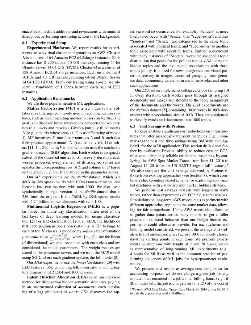
Cost Savings Results. Figure 8 and 9 show the costsavings and run-time for three different configurations forjobs of 2 hours and 20 hours, respectively, relative to run-ning on 64 on-demand machines from Cluster-A: (1) thestandard bidding strategy combined with the checkpointing-based scheme (blue). (2) the standard bidding strategy com-bined with AgileML, allowing evaluation of the incremen-tal benefit of AgileML over the checkpointing-based scheme(green). (3) Proteus which combines BidBrain and AgileML(red). Comparing Proteus to the second configuration al-lows evaluation of the additional benefit of BidBrain overthe standard bidding strategy.

The results demonstrate that Proteus significantly reducesboth cost and run-times. On average, Proteus reduces cost by83%–85% compared to traditional execution on on-demandmachines and by 42%–47% compared to the state-of-the-art approach (Standard+Checkpoint). In addition to signif-icantly lowering costs, Proteus also reduces run-times by32%–43%. The results also show that each of BidBrain andAgileML contribute significantly to Proteus’ overall cost andruntime improvements.

Attribution of Benefits. Proteus’ superior performancearises from several factors. AgileML’s ability to performagile elasticity, ability to efficiently handle evictions, andlack of run-time overhead reduces the cost by 18%–20%compared to the checkpointing-based scheme (see blueand green bars in Figure 8 and 9). Similar benefits areseen when evaluating AgileML vs. the checkpointing-basedscheme combined with BidBrain. The remaining improve-ments come from BidBrain’s ability to effectively exploitthe spot market. BidBrain reduces cost and run-time by pro-viding opportunities for free computing and projecting howresource allocations impact work throughput.

0

40

80

120

160M

achi

ne H

ours

On−DemandSpotFree

Standard + Checkpointing

ProteusOn-Demand

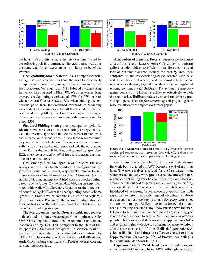
Figure 10: Breakdown of machine hours (for 2-hour jobs) amongon-demand resources, spot resources (not evicted), and free re-sources (spot resources evicted prior to end of billing hour).

Free computing occurs when an allocation produces use-ful work but is evicted by AWS before the end of a billinghour. The user receives a refund for the last partial hour,which means that any work produced by the allocation dur-ing the current billing hour has no cost to the user. Users in-crease their likelihood of getting free computing by biddingcloser to the current spot market price, which increases thelikelihood of evictions. When executing applications withsignificant eviction overheads, regularly bidding just abovethe current market price hoping to gain free computing is notan effective strategy. BidBrain accounts for eviction over-heads in making decisions about how much above the mar-ket price to bid. We experimented with always bidding justabove the market price to acquire free computing as often aspossible, but it increased the run-time of applications (3-4x)and resulted higher cost due to suffering too many evictionsafter too short a period of time. BidBrain’s predictions ofeviction likelihood and times are effective enough to find ahappy medium. On average, 32% of Proteus’ computing isfree computing, as shown in Fig. 10.

Experiments in the Wild. In addition to simulations, weran a number of Proteus jobs on AWS. Although the results

0

5

10

15

20

25Ti

me

per i

tera

tion

(sec

)

4 ParamServs16 ParamServs32 ParamServsTraditional (High Cost)

Figure 11: AgileML stage 1 with 4–32 re-liable machines out of 64 total compared totraditional (all 64 reliable; cyan), for MF.

0

5

10

15

20

25

Tim

e pe

r ite

ratio

n (s

ec)

4 ParamServs16 ActivePS32 ActivePS48 ActivePSTraditional (High Cost)

Figure 12: AgileML stage 2 with 4 reliableand 60 transient compared to stage 1 (sameratio; magenta) and traditional (64 reliable).

01234567

Tim

e pe

r ite

ratio

n (s

ec)

Workers on ReliableNo workers on ReliableTraditional (High Cost)

Figure 13: AgileML stage 3 (red) with 1reliable and 63 transient compared to stage 2(same ratio; blue) and traditional.

cover a much smaller sample size than our simulations, theobserved behavior is consistent with the simulation results.

6.4 Efficiency with AgileML TieringAgileML enables execution on a mix of reliable and tran-

sient machines, and efficient scale-up and scale-down, whilealways maintaining state required for continued operation onreliable machines. To avoid the reliable machines becominga bottleneck, AgileML uses three stages of functionality par-titioning (see Section 3.2), decreasing reliance on reliablemachines as the ratio of transient to reliable increases. (Ofcourse, higher ratios are better from a cost standpoint, be-cause transient machines are often 70–80% cheaper.) Thissection evaluates AgileML’s performance relative to the tra-ditional parameter-server architecture run entirely on high-cost reliable machines, in which all functionality (workerand parameter server) is partitioned among all machines,showing that AgileML avoids performance loss at least toa ratio of 63 transient machines to 1 reliable machine. Allresults in this section are for the MF application with theNetflix data set on Cluster-A, but results for the other appli-cations and Cluster-B are consistent and omitted only due tospace constraints.

Stage 1: Parameter Servers only on Reliable Ma-chines. The first stage spreads the parameter server acrossthe reliable machines, rather than all machines, using tran-sient machines only for worker processes.

Figure 11 shows the time-per-iteration for different num-bers of machines running parameter server shards (Param-Servs) in a 64-machine Cluster-A, representing different ra-tios of transient to reliable machines under the stage 1 con-figuration. All 64 machines run workers. The 64 Param-Serv case, which is labeled “Traditional” in the graph, rep-resents the traditional parameter server architecture in whichall machines are reliable and run both worker and parameterserver processes. The results show that stage 1 has negligi-ble slowdown for a small ratio (e.g., 1:1, represented by “32ParamServ”) of transient to reliable machines, but introducessignificant slowdown as the ratio increases. The slowdownis caused by network bottlenecks caused by many workerscommunicating with a relatively smaller number of Param-Servs.

Stage 2: ActivePSs on Transient Machines and Back-upPSs on Reliable Machines. To avoid the network bottle-neck for higher ratios, stage 2 switches to a tiered primary-backup model, using reliable machines for continuity but

not requiring them to serve as active parameter servers fora much larger number of workers.

Figure 12 shows the time-per-iteration for different con-figurations in a 64-machine Cluster-A that consists of 4 re-liable machines and 60 transient machines. The “4 Param-Servs” and “Traditional” bars described above for Figure 11are included as well, for comparison. The other three barsrepresent running ActivePSs on different numbers of tran-sient machines, together with BackupPSs on the 4 reliablemachines. All 64 machines run worker processes, in eachcase. The results show that the ActivePS-based architecturewith 32 ActivePSs introduces ≈18% slowdown comparedto the traditional parameter-server architecture, when usinga 15:1 ratio of transient to reliable machines. This slowdowndoes not occur at 7:1 and represents the beginning of thestraggler problem addressed by stage 3.

Stage 3: No Workers on Reliable Machines. When theratio of transient to reliable machines increases beyond 15:1,we observe even larger slowdowns for AgileML stage 2 rel-ative to the traditional parameter-server architecture. Thisslowdown is caused by the workers running on reliable ma-chines becoming stragglers; the network load of runningBackupPSs for a much larger number of ActivePSs inter-feres with worker communication. To solve this problem,stage 3 does not run workers on the reliable machines whenthe ratio is very high. While this reduces aggregate workercomputation power, stage 3 is only used when the reductionis small because the fraction of reliable machines is low.

Fig. 13 shows time-per-iteration with and without work-ers on the one reliable machine in a 64-machine Cluster-A that consists of 1 reliable machine and 63 transient ma-chines. The one reliable machine runs only a BackupPS. The“Traditional” bar is again shown for comparison. The resultsshow that, by shutting down reliable machine workers oncethey become stragglers, AgileML is able to match the per-formance of the traditional parameter-server architecture ata 63:1 ratio of transient to reliable machines.

Stage 3 provides the best performance only as the ratioof transient vs. reliable machines increases. Thus, all threestages are needed for AgileML to achieve high performanceacross a range of possible ratios. To illustrate, Fig. 14 com-pares time-per-iteration attained with the same footprint (8reliable + 8 transient machines), but in two different modal-ities: stage 2 and stage 3. Stage 2 is clearly best for this 1:1ratio, unlike Fig. 13, where the ratio was 63:1.

0

10

20

30

40Ti

me

per i

tera

tion

(sec

)

Stage 2Stage 3

Figure 14: AgileML running on 8 reliable and 8 transient machinesin stage 2 and stage 3 mode. Stage 2 is better for lower transient-to-reliable ratios.

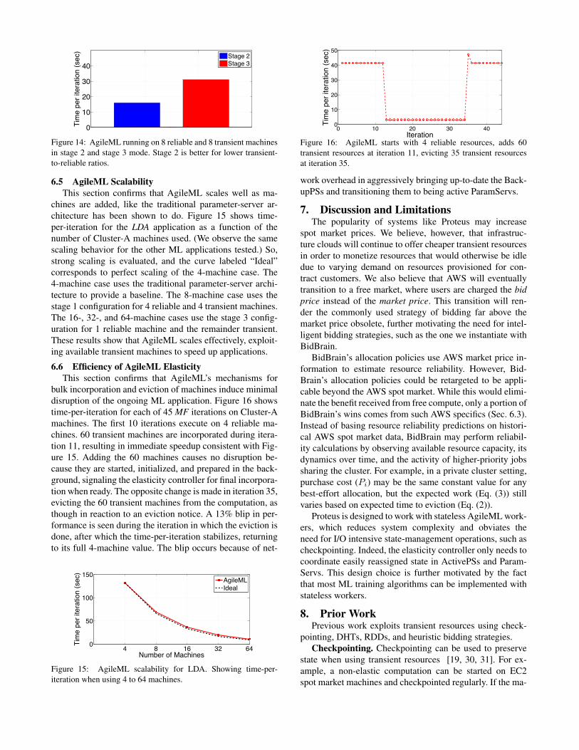
6.5 AgileML ScalabilityThis section confirms that AgileML scales well as ma-

chines are added, like the traditional parameter-server ar-chitecture has been shown to do. Figure 15 shows time-per-iteration for the LDA application as a function of thenumber of Cluster-A machines used. (We observe the samescaling behavior for the other ML applications tested.) So,strong scaling is evaluated, and the curve labeled “Ideal”corresponds to perfect scaling of the 4-machine case. The4-machine case uses the traditional parameter-server archi-tecture to provide a baseline. The 8-machine case uses thestage 1 configuration for 4 reliable and 4 transient machines.The 16-, 32-, and 64-machine cases use the stage 3 config-uration for 1 reliable machine and the remainder transient.These results show that AgileML scales effectively, exploit-ing available transient machines to speed up applications.

6.6 Efficiency of AgileML ElasticityThis section confirms that AgileML’s mechanisms for

bulk incorporation and eviction of machines induce minimaldisruption of the ongoing ML application. Figure 16 showstime-per-iteration for each of 45 MF iterations on Cluster-Amachines. The first 10 iterations execute on 4 reliable ma-chines. 60 transient machines are incorporated during itera-tion 11, resulting in immediate speedup consistent with Fig-ure 15. Adding the 60 machines causes no disruption be-cause they are started, initialized, and prepared in the back-ground, signaling the elasticity controller for final incorpora-tion when ready. The opposite change is made in iteration 35,evicting the 60 transient machines from the computation, asthough in reaction to an eviction notice. A 13% blip in per-formance is seen during the iteration in which the eviction isdone, after which the time-per-iteration stabilizes, returningto its full 4-machine value. The blip occurs because of net-

4 8 16 32 640

50

100

150

Number of Machines

Tim

e pe

r ite

ratio

n (s

ec)

AgileMLIdeal

Figure 15: AgileML scalability for LDA. Showing time-per-iteration when using 4 to 64 machines.

0 10 20 30 400

10

20

30

40

50

Iteration

Tim

e pe

r ite

ratio

n (s

ec)

Figure 16: AgileML starts with 4 reliable resources, adds 60transient resources at iteration 11, evicting 35 transient resourcesat iteration 35.

work overhead in aggressively bringing up-to-date the Back-upPSs and transitioning them to being active ParamServs.

7. Discussion and LimitationsThe popularity of systems like Proteus may increase

spot market prices. We believe, however, that infrastruc-ture clouds will continue to offer cheaper transient resourcesin order to monetize resources that would otherwise be idledue to varying demand on resources provisioned for con-tract customers. We also believe that AWS will eventuallytransition to a free market, where users are charged the bidprice instead of the market price. This transition will ren-der the commonly used strategy of bidding far above themarket price obsolete, further motivating the need for intel-ligent bidding strategies, such as the one we instantiate withBidBrain.

BidBrain’s allocation policies use AWS market price in-formation to estimate resource reliability. However, Bid-Brain’s allocation policies could be retargeted to be appli-cable beyond the AWS spot market. While this would elimi-nate the benefit received from free compute, only a portion ofBidBrain’s wins comes from such AWS specifics (Sec. 6.3).Instead of basing resource reliability predictions on histori-cal AWS spot market data, BidBrain may perform reliabil-ity calculations by observing available resource capacity, itsdynamics over time, and the activity of higher-priority jobssharing the cluster. For example, in a private cluster setting,purchase cost (Pi) may be the same constant value for anybest-effort allocation, but the expected work (Eq. (3)) stillvaries based on expected time to eviction (Eq. (2)).

Proteus is designed to work with stateless AgileML work-ers, which reduces system complexity and obviates theneed for I/O intensive state-management operations, such ascheckpointing. Indeed, the elasticity controller only needs tocoordinate easily reassigned state in ActivePSs and Param-Servs. This design choice is further motivated by the factthat most ML training algorithms can be implemented withstateless workers.

8. Prior WorkPrevious work exploits transient resources using check-

pointing, DHTs, RDDs, and heuristic bidding strategies.Checkpointing. Checkpointing can be used to preserve

state when using transient resources [19, 30, 31]. For ex-ample, a non-elastic computation can be started on EC2spot market machines and checkpointed regularly. If the ma-

chines are revoked, the computation can be restarted on an-other set of machines from the last completed checkpoint.Gupta et al. [19] propose this approach for scientific com-putations. Parameter server architectures such as Tensor-Flow [6], MxNet [9], Petuum [37], LazyTables [11], andIterStore [12] provide no explicit mechanism for exploitingtransient resources, and hence would likewise rely on check-pointing. A single machine failure causes most of these sys-tems to restart an ongoing computation from the most re-cent checkpoint.9 Although this is reasonable in small-to-medium clusters under traditional failure models, it can incurhigh overheads in elastic settings due to the frequency of re-vocations (e.g., all the spikes in Figure 3). Moreover, dynam-ically adding machines to running ML applications is notsupported by these frameworks. To do so would seem to re-quire stopping the computation in a consistent state, addingthe resources, adjusting the mapping of computation tasksto machines and copying any needed state accordingly, andthen restarting. (Section 3.3 describes AgileML’s alternative,efficient approach.) We hope this work will motivate otherML frameworks to become agile elastic, and when they do,we believe they will integrate well with BidBrain and pro-vide a great comparison for AgileML. In our experimentalstudy, we compare Proteus’ explicit elasticity support to thischeckpointing-based approach.

Distributed Hash Tables (DHTs). The parameter serversystem described by Li et al. [25] includes support for addingand removing machines during execution. To realize this fea-ture, the system uses a direct-mapped DHT design based onconsistent hashing, wherein each parameter server process isresponsible for a particular key range, and parameter valuereplication. Protocols for adding and removing machines aredescribed. While DHTs are effective for adding or removingresources one-at-a-time, we believe that Proteus’ approachto elasticity is better suited to the bulk addition and removalof nodes that characterize the transient resource availabil-ity discussed above. Li et al. did not evaluate the speed ofnode set changes, but we expect that it would be insufficientto address revocation of a sizable subset of cheap machineswithin the limited warning period provided. The replicationmechanism also would not solve this issue, because bulk re-vocation is akin to correlated failure of many nodes, whilethe mechanism is designed for independent failures.

Spark and RDDs. Spark achieves fault tolerance withRDDs, storing deterministic transformations for subsequentreplay on recovery from checkpoint. Flint [30], concurrentlywith our work, proposed a system for running Spark appli-cations on transient machines. Unlike our tiered approachleveraging a mix of transient and non-transient machinessimultaneously, Flint runs ML workloads entirely on tran-sient nodes,10 like the checkpointing approach above. RDDs9 Tensorflow has a mechanism for handling single machine failures via itsstraggler mitigation mechanism.10 or entirely on non-transient nodes in the rare cases when they are cheaper

reduce the cost of checkpointing/recovery for Spark appli-cations by selectively choosing the set of RDDs needed.Whereas Flint relies heavily on the Spark’s computing modelin exploiting transient machines, AgileML enables exploita-tion of such resources for parameter server systems, whichare different and much more efficient for iterative conver-gent ML (Sec. 2.1). Furthermore, Proteus’ aggressive allo-cation strategy on the spot market provides significant sav-ings, including 32% free computing on average. In contrast,Flint only considers switching when current resources arerevoked and only bids the on-demand price, correspondingto Standard+AgileML in our graphs.

Bidding Strategies. Bidding strategies for EC2 spot in-stances have been studied [7, 32, 39]. Agmon et al. [7] showminimal correlation between near term AWS spot prices andspot instance availability. Marathe et al. [28] propose us-ing redundancy across AWS zones for HPC computationson EC2. For interactive workloads, Flint [30] seeks to di-versify across zones and machine classes to minimize revo-cation probability. Spot Fleet EC2, an AWS service, allowsusers to specify a resource capacity target and automaticallymaintain that target, replacing evicted instances. It is appli-cation agnostic, however, and does not take into account anyapplication-level concerns, such as maximizing performanceper unit cost. By default, Spot Fleet follows the same config-ured strategy as the standard bidding policy, bidding the on-demand price on the currently cheapest available resource(Sec. 6.3). We show significant improvements over such abidding strategy.

9. SummaryProteus aggressively exploits transient revocable ma-

chines to complete ML model training faster and cheaper.For example, Proteus can exploit EC2’s spot market to save≈85% compared to using only on-demand machines. Bycombining non-transient (e.g., on-demand) and transient(spot) machines, Proteus can rapidly and efficiently incor-porate transient resources and deal with revocations, whichcombines with its aggressive allocation strategy to save≈50% compared to a state-of-the-art checkpointing-basedapproach using a standard spot market bidding strategy.

AcknowledgmentsWe thank Steven Hand for shepherding this paper, and we thank

the members and companies of the PDL Consortium: Broadcom,Citadel, Dell EMC, Google, HP Labs, Hitachi, Intel, Microsoft Re-search, MongoDB, NetApp, Oracle, Samsung, Seagate Technol-ogy, Tintri, Two Sigma, Uber, Veritas and Western Digital for theirinterest, insights, feedback, and support. This research is supportedin part by Intel as part of the Intel Science and Technology Cen-ter for Visual Cloud Systems (ISTC-VCS), National Science Foun-dation under awards CNS-1042537, CCF-1533858, CNS-1042543(PRObE [15]) and DARPA Grant FA87501220324.

References[1] AWS EC2. http://aws.amazon.com/ec2/.

[2] Spot Bid Advisor. https://aws.amazon.com/ec2/spot/

bid-advisor/.

[3] Google Compute Engine. https://cloud.google.com/

compute/.

[4] Apache Hadoop. http://hadoop.apache.org/.

[5] New York Times dataset. http://www.ldc.upenn.edu/.

[6] M. Abadi, P. Barham, J. Chen, Z. Chen, A. Davis, J. Dean,M. Devin, S. Ghemawat, G. Irving, M. Isard, M. Kudlur,J. Levenberg, R. Monga, S. Moore, D. G. Murray, B. Steiner,P. Tucker, V. Vasudevan, P. Warden, M. Wicke, Y. Yu, andX. Zheng. Tensorflow: A system for large-scale machinelearning. In Proceedings of the 12th USENIX Conference onOperating Systems Design and Implementation (OSDI 16).

[7] O. Agmon Ben-Yehuda, M. Ben-Yehuda, A. Schuster, andD. Tsafrir. Deconstructing Amazon EC2 spot instance pricing.ACM Transactions on Economics and Computation, 1(3):16,2013.

[8] C. M. Bishop. Pattern Recognition and Machine Learning(Information Science and Statistics). Springer-Verlag NewYork, Inc., Secaucus, NJ, USA, 2006. ISBN 0387310738.

[9] T. Chen, M. Li, Y. Li, M. Lin, N. Wang, M. Wang, T. Xiao,B. Xu, C. Zhang, and Z. Zhang. MXNet: A flexible and ef-ficient machine learning library for heterogeneous distributedsystems. arXiv preprint arXiv:1512.01274, 2015.

[10] T. Chilimbi, Y. Suzue, J. Apacible, and K. Kalyanaraman.Project Adam: Building an efficient and scalable deep learn-ing training system. In Proceedings of the 11th USENIXConference on Operating Systems Design and Implementation(OSDI 14), pages 571–582, 2014.

[11] H. Cui, J. Cipar, Q. Ho, J. K. Kim, S. Lee, A. Kumar, J. Wei,W. Dai, G. R. Ganger, P. B. Gibbons, G. A. Gibson, andE. P. Xing. Exploiting bounded staleness to speed up bigdata analytics. In Proceedings of the 2014 USENIX AnnualTechnical Conference (USENIX ATC 14), pages 37–48, 2014.

[12] H. Cui, A. Tumanov, J. Wei, L. Xu, W. Dai, J. Haber-Kucharsky, Q. Ho, G. R. Ganger, P. B. Gibbons, G. A. Gib-son, and E. P. Xing. Exploiting iterative-ness for parallel MLcomputations. In Proceedings of the 5th ACM Symposium onCloud Computing (SoCC 14), pages 1–14. ACM, 2014.

[13] C. Curino, D. E. Difallah, C. Douglas, S. Krishnan, R. Ra-makrishnan, and S. Rao. Reservation-based scheduling: Ifyou’re late don’t blame us! In Proceedings of the 5th ACMSymposium on Cloud Computing (SoCC 14), pages 1–14.ACM, 2014.

[14] R. Gemulla, E. Nijkamp, P. J. Haas, and Y. Sismanis. Large-scale matrix factorization with distributed stochastic gradientdescent. In Proceedings of the 17th Conference on KnowledgeDiscovery and Data Mining (KDD 11), 2011.

[15] G. Gibson, G. Grider, A. Jacobson, and W. Lloyd. Probe:A thousand-node experimental cluster for computer systemsresearch. USENIX, 38(3), 2013.

[16] J. E. Gonzalez, Y. Low, H. Gu, D. Bickson, and C. Guestrin.PowerGraph: Distributed graph-parallel computation on nat-

ural graphs. In Proceedings of the 10th USENIX Symposiumon Operating Systems Design and Implementation (OSDI 12),2012.

[17] J. E. Gonzalez, R. S. Xin, A. Dave, D. Crankshaw, M. J.Franklin, and I. Stoica. GraphX: Graph processing in a dis-tributed dataflow framework. In Proceedings of the 11thUSENIX Symposium on Operating Systems Design and Im-plementation (OSDI 14), pages 599–613, 2014.

[18] T. L. Griffiths and M. Steyvers. Finding scientific topics. Pro-ceedings of the National Academy of Sciences of the UnitedStates of America, 2004.

[19] A. Gupta, B. Acun, O. Sarood, and L. V. Kale. Towardsrealizing the potential of malleable jobs. In Proceedingsof the 21st International Conference on High PerformanceComputing (HiPC 14), pages 1–10. IEEE, 2014.

[20] A. Harlap, H. Cui, W. Dai, J. Wei, G. R. Ganger, P. B. Gib-bons, G. A. Gibson, and E. P. Xing. Addressing the stragglerproblem for iterative convergent parallel ml. In Proceedingsof the 7th ACM Symposium on Cloud Computing (SoCC 16),pages 98–111. ACM, 2016.

[21] B. Hindman, A. Konwinski, M. Zaharia, A. Ghodsi, A. D.Joseph, R. H. Katz, S. Shenker, and I. Stoica. Mesos: Aplatform for fine-grained resource sharing in the data center.In Proceedings of the 8th USENIX Symposium on NetworkedSystems Design and Implementation (NSDI 11), volume 11,pages 22–22, 2011.

[22] Q. Ho, J. Cipar, H. Cui, S. Lee, J. K. Kim, P. B. Gibbons,G. A. Gibson, G. R. Ganger, and E. P. Xing. More effectivedistributed ML via a Stale Synchronous Parallel parameterserver. In Proceedings of the Advances in Neural InformationProcessing Systems (NIPS 13), 2013.

[23] A. Krizhevsky, I. Sutskever, and G. E. Hinton. Imagenetclassification with deep convolutional neural networks. InAdvances in neural information processing systems, pages1097–1105, 2012.

[24] J. Langford, A. J. Smola, and M. Zinkevich. Slow learners arefast. In Proceedings of the 23rd Annual Conference on NeuralInformation Processing Systems (NIPS 09), 2009.

[25] M. Li, D. G. Andersen, J. W. Park, A. J. Smola, A. Ahmed,V. Josifovski, J. Long, E. J. Shekita, and B.-Y. Su. Scalingdistributed machine learning with the parameter server. InProceedings of the 11th USENIX Symposium on OperatingSystems Design and Implementation (OSDI 14), pages 583–598, 2014.

[26] J. Liu, J. Chen, and J. Ye. Large-scale sparse logistic regres-sion. In Proceedings of the 15th ACM SIGKDD internationalconference on Knowledge discovery and data mining, pages547–556. ACM, 2009.

[27] Y. Low, J. Gonzalez, A. Kyrola, D. Bickson, C. Guestrin,and J. M. Hellerstein. GraphLab: A new parallel frameworkfor machine learning. In Proceedings of the Conference onUncertainty in Artificial Intelligence (UAI), 2010.

[28] A. Marathe, R. Harris, D. Lowenthal, B. R. De Supinski,B. Rountree, and M. Schulz. Exploiting redundancy for cost-effective, time-constrained execution of HPC applications onAmazon EC2. In Proceedings of the 23rd international sym-

posium on High-performance parallel and distributed com-puting, pages 279–290. ACM, 2014.

[29] O. Russakovsky, J. Deng, H. Su, J. Krause, S. Satheesh, S. Ma,Z. Huang, A. Karpathy, A. Khosla, M. Bernstein, A. C. Berg,and L. Fei-Fei. ImageNet Large Scale Visual RecognitionChallenge, 2014.

[30] P. Sharma, T. Guo, X. He, D. Irwin, and P. Shenoy.Flint: Batch-interactive data-intensive processing on transientservers. In Proceedings of the 11th European Conference onComputer Systems (EuroSys 16), page 6. ACM, 2016.

[31] S. Subramanya, T. Guo, P. Sharma, D. Irwin, and P. Shenoy.Spoton: a batch computing service for the spot market. In Pro-ceedings of the Sixth ACM Symposium on Cloud Computing(SoCC 15), pages 329–341. ACM, 2015.

[32] S. Tang, J. Yuan, and X.-Y. Li. Towards optimal bidding strat-egy for Amazon EC2 cloud spot instance. In Proceedingsof the 5th IEEE International Conference on Cloud Comput-ing(CLOUD 12), pages 91–98. IEEE, 2012.

[33] V. K. Vavilapalli, A. C. Murthy, C. Douglas, S. Agarwal,M. Konar, R. Evans, T. Graves, J. Lowe, H. Shah, S. Seth,, B. Saha, C. Curino, O. O’Malley, S. Radia, B. Reed, andE. Baldeschwieler. Apache hadoop yarn: Yet another resourcenegotiator. In Proceedings of the 4th Annual Symposium onCloud Computing (SoCC 13), page 5. ACM, 2013.

[34] A. Verma, L. Pedrosa, M. Korupolu, D. Oppenheimer,E. Tune, and J. Wilkes. Large-scale cluster management atGoogle with Borg. In Proceedings of the 10th European Con-ference on Computer Systems (EuroSys 15), page 18. ACM,2015.

[35] J. Wang, J. Yang, K. Yu, F. Lv, T. Huang, and Y. Gong.Locality-constrained linear coding for image classification. InProceedings of the Computer Vision and Pattern Recognition(CVPR), 2010 IEEE Conference on, pages 3360–3367. IEEE,2010.

[36] J. Wei, W. Dai, A. Qiao, Q. Ho, H. Cui, G. R. Ganger, P. B.Gibbons, G. A. Gibson, and E. P. Xing. Managed communi-cation and consistency for fast data-parallel iterative analytics.In Proceedings of the 6th ACM Symposium on Cloud Comput-ing (SoCC 15), pages 381–394. ACM, 2015.

[37] E. P. Xing, Q. Ho, W. Dai, J. K. Kim, J. Wei, S. Lee, X. Zheng,P. Xie, A. Kumar, and Y. Yu. Petuum: A new platform fordistributed machine learning on big data. In Proceedingsof the 22th Conference on Knowledge Discovery and DataMining (KDD 15), pages 1335–1344. ACM, 2015.

[38] M. Zaharia, M. Chowdhury, M. J. Franklin, S. Shenker, andI. Stoica. Spark: Cluster computing with working sets. Pro-ceedings of the 2nd USENIX Workshop on Hot Topics in CloudComputing (HotCloud 10), 10:10–10, 2010.

[39] L. Zheng, C. Joe-Wong, C. W. Tan, M. Chiang, and X. Wang.How to bid the cloud. In Proceedings of the 2015 ACM Con-ference on Special Interest Group on Data Communication,pages 71–84. ACM, 2015.