protein function prediction with semi-supervised...
TRANSCRIPT

Protein function prediction with
semi-supervised classification based on
evolutionary multi-objective optimization
Jorge Alberto Jaramillo Garzón
Advisors
César Germán Castellanos Domínguez, PhD.
Alexandre Perera i Lluna, PhD.
Doctoral Program on Engineering - Automatics
Universidad Nacional de Colombia sede Manizales
This document is presented in partial fulfillment of the requirements for the
degree of
Doctor of Philosophy
2013

Predicción de funciones de proteínas
usando clasificación semi-supervisada
basada en técnicas de optimización
multi-objetivo
Jorge Alberto Jaramillo Garzón
Directores
César Germán Castellanos Domínguez, PhD.
Alexandre Perera i Lluna, PhD.
Doctorado en Ingeniería - Linea Automática
Universidad Nacional de Colombia sede Manizales
Este documento se presenta como requisito parcial para obtener el grado de
Doctor en filosofía
2013

This Thesis was typeset by the author using LATEX2ε.
Copyright c©2013 by Universidad Nacional de Colombia. All rights reserved.
No part of this publication may be reproduced or transmitted in any form or
by any means, electronic or mechanical, including photocopy, recording, or any
information storage and retrieval system, without permission in writing from the
author.
Department: Ingeniería Eléctrica, Electrónica y ComputaciónUniversidad Nacional de Colombia sede Manizales, Colombia.
PhD Thesis: Protein function prediction with semi-supervisedclassification based on multi-objective optimization
Author: Jorge Alberto Jaramillo GarzónElectronic Engineer and Master in Engineering- Industrial Automation
Advisor: Germán Castellanos Domínguez, PhD.Universidad Nacional de Colombia sede Manizales
Co-advisor Alexandre Perera i LlunaUniversitat Politècnica de Catalunya
Year: 2013
Committe: Carolina Ruiz Carrizosa, PhD.Worcester Polytechnic Institute, United States of America.
Claudia Consuelo Rubiano Castellanos, PhD.Universidad Nacional de Colombia, Colombia.
Andrés Mauricio Pinzón Velasco, PhD.Centro de Bioinformática y Biología Computacional, Colombia.
After the defense of the PhD dissertation at Universidad Nacional
de Colombia, sede Manizales, the jury agrees to grant the following
qualification:
Manizales, November 25th, 2013.
Carolina RuizCarrizosa
Claudia Consuelo RubianoCastellanos
Andrés Mauricio PinzónVelasco

This work was partially supported by the Spanish Ministerio de Ed-
ucación y Ciencia under the Ramón y Cajal Program and the grants
TEC2010-20886-C02-02 and TEC2010-20886-C02-01, by Centro de
Investigación Biomédica en Red en Bioingeniería, Biomateriales y
Nanomedicina (CIBER-BBN), by Dirección de Investigaciones de Man-
izales (DIMA) from Universidad Nacional de Colombia through the
Convocatoria nacional de investigación 2009, modalidad apoyo a Tesis
de postgrado and by the Colombian National Research Institute (COL-
CIENCIAS) under grant 111952128388.

Aknowledgements
First, I would like to thank Professor Alexandre Perera i Lluna , who was co-
director of this work and who introduced me to the area of bioinformatics, for all
the support he gave me, for his teachings and because his spirit and disposition
towards his students have been a great example for me. His ideas and knowledge
set the course of this work and therefore my academic life in the past years
through its development, and most likely his influence will be also reflected in the
coming years. For all these things and for his friendship, thank you very much.
I also want to thank Professor César Germán Castellanos Domínguez, co-
director of this work and who has been my mentor for more than eight years
ago. His influence on me and on all the people who in one way or another have
made the Group of Control and Digital Signal Processing, has set a precedent
and strengthened the research in Colombia. I really appreciate all his teachings
and every opportunity he has given me over the years.
I also thank my colleagues in the Grupo de Control y Procesamiento Digital
de Señales at Universidad Nacional de Colombia, sede Manizales, who accom-
panied me during this time. I especially want to thank my great friend Julián
David Arias Londoño, companion of many battles throughout the years we have
shared together and who until the end of this work remained selfless giving me
encouragement and help. I should also mention Mauricio Orozco Alzate, who
gave me the first contacts and ideas to start with the topic of this work and
therefore had a great influence on his development. Also, I want to immensely
thank Andrés Felipe Giraldo Forero, who became my right hand in the the devel-
opment of this work in the recent years and who I would predict a bright future in
research. Also, thanks to Gustavo Alonso Arango Argoty and Sebastián García
iii
López, their contributions were very important and I appreciate the dedication
that each one had in their work.
I thank the members of the group of Biomedical Signals and Systems at the
Universidad Politécnica de Cataluña, particularly in the group g-SISBIO, whose
contributions and discussions were of great help to me. I especially thank Joan
Josep Gallardo Chacón, Andrey Ziyatdinov, Helena Brunel Montaner, Raimon
Massanet Vila and Joan Maynou Fernández. I also want to thank Professor
Montserrat Vallverdú Ferrer for her support and concern during my visits to the
UPC, as well as for being the mediator so that I could make contact with Professor
Alexandre Perera and his group.
On the other hand , I want to thank my mom, María del Rocío Garzón
Hernández, who has been my main example throughout my life and who with his
care and affection has made me everything I am. Each one of my achievements
is also hers.
I also thank Clara Sofía Obando Alzate , with whom I have shared my life for
the past thirteen years and which love and support has helped me to continue
during this time. She has been the person who has more closely followed (and
suffered) this work with me. For all these things, for each of the moments we
have shared and each of absences she has tolerated me, thank you very much.
I especially want to mention several of my friends, who encouraged me and
accompanied me throughout the development of this work: Julián Andrés Largo
Trejos, César Johny Rugeles Mosquera, Carlos Guillermo Caicedo Erazo (and the
little pig R.I.P.), Luis Bernardo Monroy Jaramillo, Jorge Iván Montes Monsalve,
Julián David Santa González and John Eder Cuitiva Sánchez. His words of
encouragement and his company were of great importance in many moments.
Finally, I thank my current colleagues at Instituto Tecnológico Metropoli-
tano, who have also contributed with their support and motivation to the com-
pletion of this work. Special thanks to Edilson Delgado Trejos, francisco Eugenio
López Giraldo, Leonardo Duque Muñoz, Delio Augusto Aristizábal Martínez, Al-
fredo Ocampo Hurtado, Norma Patricia Guarnizo Cutiva, Germán David Góez
Sánchez, Hermes Alexánder Fandiño Toro , Fredy Andrés Torres Muñoz, Juan
Carlos Rodríguez Gamboa and Eva Susana Albarracín Estrada.
iv

To all of them and all the people that influenced the development of this work
in one way or another, ¡thank you!.
Jorge Alberto Jaramillo Garzón
November 2013
v

vi

Agradecimientos
En primer lugar quisiera agradecerle al profesor Alexandre Perera i Lluna, quien
fue co-director de este trabajo y quien me introdujo en el área de la bioinformática,
por todo el apoyo que me brindó, por sus enseñanzas y porque su espíritu y
disposición para con sus estudiantes han sido un gran ejemplo para mí. Sus ideas
y su conocimiento trazaron el rumbo de este trabajo y por lo tanto encaminaron
mi vida académica durante los años transcurridos en el desarrollo de éste y muy
seguramente esa influencia se reflejará también en los años venideros. Por todo
esto y por su amistad, muchas gracias.
También quiero agradecer al profesor César Germán Castellanos Domínguez,
co-director de este trabajo y quien ha sido mi tutor desde hace más de ocho años.
Su influencia sobre mí, y sobre todas las personas que de una u otra forma hemos
hecho parte del Grupo de Control y Procesamiento Digital de Señales, ha marcado
un precedente y ha fortalecido la investigación en Colombia. Le agradezco mucho
todas sus enseñanzas y todas las oportunidades que me ha brindado durante estos
años.
Agradezco también a mis compañeros del Grupo de Control y Procesamiento
Digital de Señales de la Universidad Nacional de Colombia, sede Manizales,
quienes me acompañaron durante todo este tiempo. Especialmente, quiero agrade-
cer a mi gran amigo Julián David Arias Londoño, compañero de muchas batallas
durante todos los años que hemos compartido juntos y quien hasta el final de
este trabajo permaneció brindándome su aliento y ayuda desinteresada. Quiero
mencionar también a Mauricio Orozco Alzate, quien me proporcionó los primeros
contactos e ideas para comenzar con el tema de este trabajo y por lo tanto tuvo
una gran influencia sobre su desarrollo. Además, quiero agradecer inmensamente
vii

a Andrés Felipe Giraldo Forero, quien se convirtió en mi mano derecha en los últi-
mos años del desarrollo de este trabajo y a quien le auguro un futuro brillante en
la investigación. Igualmente a Gustavo Alonso Arango Argoty y Sebastián García
López, sus aportes fueron de gran importancia y les agradezco la dedicación que
cada uno tuvo en su trabajo.
Le agradezco a las personas del grupo de Señales y Sistemas Biomédicos de
la Universidad Politécnica de Cataluña, particularmente a los integrantes del
grupo g-SISBIO, cuyos aportes y discusiones fueron de gran ayuda para mí.
Le agradezco especialmente a Joan Josep Gallardo Chacón, Andrey Ziyatdinov,
Helena Brunel Montaner, Raimon Massanet Vila y Joan Maynou Fernández.
Además quiero agradecerle a la profesora Montserrat Vallverdú Ferrer por su
apoyo y preocupación durante mis visitas a la UPC, así como por haber sido la
mediadora para que yo pudiera establecer el contacto con el profesor Alexandre
Perera y su grupo.
Por otro lado, quiero agradecerle a mi mamá, María del Rocío Garzón Hernán-
dez, quien ha sido mi principal ejemplo durante toda mi vida y quien con sus
cuidados y su cariño ha hecho de mí todo lo que soy. Cada uno de mis logros es
también suyo.
Agradezco además a Clara Sofía Obando Alzate, con quien he compartido mi
vida durante los últimos trece años y que con su amor y su apoyo me ha ayudado
a continuar durante todo este tiempo. Ella ha sido la persona que ha seguido
(y sufrido) más de cerca este trabajo conmigo. Por todo esto, por cada uno de
los momentos que hemos compartido y por cada una de las ausencias que me ha
tolerado, muchas gracias.
Quiero mencionar especialmente a varios de mis amigos, quienes me alentaron
y acompañaron durante todo el desarrollo de este trabajo: Julián Andrés Largo
Trejos, César Johny Rugeles Mosquera, Carlos Guillermo Caicedo Erazo (y al
marranito Q.E.P.D.), Luis Bernardo Monroy Jaramillo, Jorge Iván Montes Mon-
salve, Julián David Santa González y Jhon Eder Cuitiva Sánchez. Sus palabras
de aliento y su compañía fueron de gran importancia en muchos momentos.
Finalmente, le agradezco a mis actuales compañeros del Instituto Tecnológico
Metropolitano, quienes también han contribuído con su apoyo, su motivación y
viii
ayuda a la finalización de este trabajo. Agradezco especialmente a Edilson Del-
gado Trejos, Francisco Eugenio López Giraldo, Leonardo Duque Muñoz, Delio Au-
gusto Aristizábal Martínez, Alfredo Ocampo Hurtado, Norma Patricia Guarnizo
Cutiva, Germán David Góez Sánchez, Hermes Alexánder Fandiño Toro, Fredy
Andrés Torres Muñoz, Juan Carlos Rodríguez Gamboa y Eva Susana Albarracín
Estrada.
A todos ellos y a todas las personas que influyeron de una u otra manera en
el desarrollo de este trabajo, ¡muchísimas gracias!.
Jorge Alberto Jaramillo Garzón
Noviembre de 2013
ix

x

Contents
Aknowledgements (+Agradecimientos) iii
List of Tables xv
List of Figures xx
Abstract (+Resumen) xxi
Introduction 1
Justification . . . . . . . . . . . . . . . . . . . . . . . . . . . . . . . . . 1
Problem statement . . . . . . . . . . . . . . . . . . . . . . . . . . . . . 2
Hypothesis . . . . . . . . . . . . . . . . . . . . . . . . . . . . . . . . . 4
Objectives . . . . . . . . . . . . . . . . . . . . . . . . . . . . . . . . . . 4
1 Preliminary concepts 7
1.1 Functionality of proteins and their structure levels . . . . . . . . . 7
1.2 Gene ontology . . . . . . . . . . . . . . . . . . . . . . . . . . . . . 9
1.3 Paradigms in machine learning . . . . . . . . . . . . . . . . . . . . 11
1.3.1 Supervised and unsupervised learning . . . . . . . . . . . . 11
1.3.2 Transductive, semi-unsupervised and semi-supervised learn-
ing . . . . . . . . . . . . . . . . . . . . . . . . . . . . . . . 13
1.3.3 Remarks on the application of machine learning methods
for protein function prediction . . . . . . . . . . . . . . . . 16
1.4 Single-objective and multi-objective optimization for machine learn-
ing methods . . . . . . . . . . . . . . . . . . . . . . . . . . . . . . 17
xi

Contents
2 Supervised Gene Ontology prediction for Embryophyta organ-
isms 23
2.1 Gene Ontology predictors . . . . . . . . . . . . . . . . . . . . . . 24
2.2 Proposed methodology: prediction of GO terms in Embryophyta
organisms with pattern recognition techniques . . . . . . . . . . . 26
2.2.1 Database . . . . . . . . . . . . . . . . . . . . . . . . . . . 27
2.2.2 Definition of classes . . . . . . . . . . . . . . . . . . . . . . 28
2.2.3 Characterization of protein sequences . . . . . . . . . . . . 29
2.2.4 Feature clusters . . . . . . . . . . . . . . . . . . . . . . . . 32
2.2.5 Feature selection strategy . . . . . . . . . . . . . . . . . . 32
2.2.6 Decision making . . . . . . . . . . . . . . . . . . . . . . . . 33
2.3 Results and Discussion . . . . . . . . . . . . . . . . . . . . . . . . 35
2.3.1 Analysis of predictability with individual feature clusters . 35
2.3.2 Analysis of predictability with the full set of features . . . 39
2.4 Concluding remarks . . . . . . . . . . . . . . . . . . . . . . . . . . 43
3 Semi-supervised Gene Ontology prediction for Embryophyta or-
ganisms 47
3.1 State of the art in semi-supervised classification . . . . . . . . . . 48
3.1.1 Generative methods . . . . . . . . . . . . . . . . . . . . . . 50
3.1.2 Density-based methods . . . . . . . . . . . . . . . . . . . . 51
3.1.3 Graph-based methods . . . . . . . . . . . . . . . . . . . . 53
3.1.4 Applicatons of semi-supervised learning for protein func-
tion prediction . . . . . . . . . . . . . . . . . . . . . . . . 55
3.2 Proposed methodology: semi-supervised learning for predicting
gene ontology terms in Embryophyta plants . . . . . . . . . . . . . 56
3.2.1 Selected semi-supervised algorithms . . . . . . . . . . . . . 56
3.2.2 Databases . . . . . . . . . . . . . . . . . . . . . . . . . . . 59
3.2.3 Decision making . . . . . . . . . . . . . . . . . . . . . . . . 61
3.3 Results and discussion . . . . . . . . . . . . . . . . . . . . . . . . 61
3.3.1 Analysis of benchmark datasets . . . . . . . . . . . . . . . 61
3.3.2 Analysis of GO prediction in Embryophyta plants . . . . . 62
3.4 Concluding remarks . . . . . . . . . . . . . . . . . . . . . . . . . . 69
xii

Contents
4 Semi-supervised learning with multi-objective optimization 71
4.1 Proposed method . . . . . . . . . . . . . . . . . . . . . . . . . . . 72
4.1.1 Objective functions . . . . . . . . . . . . . . . . . . . . . . 74
4.1.2 Non-linear mapping . . . . . . . . . . . . . . . . . . . . . . 75
4.2 Proposed method: multi-objective semi-supervised learning for
predicting GO terms in Embryophyta plants . . . . . . . . . . . . 76
4.2.1 Selected multi-objective strategy: cuckoo search . . . . . . 76
4.2.2 Decision making . . . . . . . . . . . . . . . . . . . . . . . . 80
4.3 Results and discussion . . . . . . . . . . . . . . . . . . . . . . . . 80
4.3.1 Analysis with the benchmark datasets . . . . . . . . . . . 81
4.3.2 Analysis of GO prediction in Embryophyta plants . . . . . 84
4.4 Concluding remarks . . . . . . . . . . . . . . . . . . . . . . . . . . 85
5 Conclusions 89
5.1 Main contributions . . . . . . . . . . . . . . . . . . . . . . . . . . 89
5.2 Future research directions . . . . . . . . . . . . . . . . . . . . . . 92
References 95
xiii


List of Tables
1.1 Examples of loss functions and the optimization methods used in
several supervised machine learning algorithms . . . . . . . . . . . 18
2.1 Definition and size of the classes. The list of GO terms covered
by this analysis is intended to provide a complete landscape of
GO predictability at the three levels of protein functionality in
Embryophyta plants. For classification purposes, classes marked
with an asterisk (*) were redefined. The number of samples in
those categories corresponds to the sequences associated to that
class and none of its also listed descendants. . . . . . . . . . . . . 30
2.2 Initial set of features extracted from amino acid sequences. Fea-
tures are divided into three broad categories: physical-chemical
features, primary structure composition statistics and secondary
structure composition statistics. . . . . . . . . . . . . . . . . . . . 31
2.3 Description of the clusters of features with similar information con-
tent . . . . . . . . . . . . . . . . . . . . . . . . . . . . . . . . . . 32
3.1 Performance over the three benchmark sets. Each position shows
“mean± standard deviation” and the corresponding p-value. High-
lighted values are significantly better than the supervised SVM. . 62
4.1 Performance over the three benchmark sets for several solutions
from the Pareto fronts. Each position shows “mean ± standard
deviation”. Highlighted values on the right are the highest among
the three individual objectives. . . . . . . . . . . . . . . . . . . . 84
xv

List of Figures
1.1 Levels of protein structure . . . . . . . . . . . . . . . . . . . . . . 9
1.2 Molecular Function ontology from the plants GO-slim. The list of
acronyms can be found in table 2.1 . . . . . . . . . . . . . . . . . 10
1.3 Example of unsupervised learning . . . . . . . . . . . . . . . . . . 12
1.4 Example of supervised learning . . . . . . . . . . . . . . . . . . . 14
1.5 Example of a Pareto front . . . . . . . . . . . . . . . . . . . . . . 20
2.1 Prediction performance with different feature clusters. Rows rep-
resent classes in Table 2.1 while columns represent feature groups
in Table 2.3. For each ontology, best predicted categories are or-
dered from top to bottom while most discriminant feature groups
are ordered from left to right. . . . . . . . . . . . . . . . . . . . . 36
2.2 Performance variation in function of the identity cutoff. Green and
blue plots show the variation of the general prediction performance
for SVM and BLASTP, respectively, according to the identity per-
centage cutoff used in the dataset. Boxplots show the dispersion
throughout the 75 GO terms. . . . . . . . . . . . . . . . . . . . . 40
2.3 Prediction performance with the complete set of features. Bars in
the left plots show sensitivity and specificity of SVMs. Lines depict
geometric mean as a global performance measure for SVM (green)
and BLASTP (blue). Right plots depict the p-values obtained by
paired t-tests at a 95% significance level. For each ontology, the
best predicted categories are ordered from top to bottom. . . . . . 42
xvii

List of Figures
2.4 Propagated prediction performance. Prediction performance when
propagating predictions of children nodes to their parents. Note
that asterisks in the category names have been removed since cat-
egories include all their member now. . . . . . . . . . . . . . . . . 44
3.1 Two-dimensional projections of the benchmark datasets. Filled cir-
cles represent labeled data while empty circles represent unlabeled
data. . . . . . . . . . . . . . . . . . . . . . . . . . . . . . . . . . . 60
3.2 Example instance from the Digit1 dataset (taken from Chapelle
and Schölkopf (2006)) . . . . . . . . . . . . . . . . . . . . . . . . 61
3.3 Comparisson between the S3VM method and the supervised SVM.
Bars in the left plots show sensitivity and specificity of the S3VM
and lines depict geometric mean for S3VM (orange) and the clas-
sical supervised SVM (green). Right plots depict the p-values ob-
tained by paired t-tests at a 95% significance level. For each on-
tology, the best predicted categories are ordered from top to bottom. 64
3.4 Comparisson between BLASTp and the S3VM method. Bars in the
left plots show sensitivity and specificity of the S3VM and lines
depict geometric mean for S3VM (orange) and BLASTp (blue).
Right plots depict the p-values obtained by paired t-tests at a 95%
significance level. For each ontology, the best predicted categories
are ordered from top to bottom. . . . . . . . . . . . . . . . . . . . 65
3.5 Comparison between the Lap-SVM method and the supervised
SVM. Bars in the left plots show sensitivity and specificity of the
Lap-SVM and lines depict geometric mean for Lap-SVM (orange)
and the classical supervised SVM (green). Right plots depict the
p-values obtained by paired t-tests at a 95% significance level. For
each ontology, the best predicted categories are ordered from top
to bottom. . . . . . . . . . . . . . . . . . . . . . . . . . . . . . . . 67
xviii

List of Figures
3.6 Comparison between BLASTp and the Lap-SVM method. Bars in
the left plots show sensitivity and specificity of the Lap-SVM and
lines depict geometric mean for Lap-SVM (orange) and BLASTp
(blue). Right plots depict the p-values obtained by paired t-tests
at a 95% significance level. For each ontology, the best predicted
categories are ordered from top to bottom. . . . . . . . . . . . . . 68
4.1 Example of three Lévy flights of length 100 starting from the origin 78
4.2 Flow diagram of the proposed methodology. The green area high-
lights the training process . . . . . . . . . . . . . . . . . . . . . . 81
4.3 Pareto front for the g241n benchmark dataset. The yellow, orange
and green dots depict the minima for the the manifold, cluster
and supervised objectives, respectively. The red dot depicts the
most feasible solution according to the class labels, found by the
cross-validation procedure. . . . . . . . . . . . . . . . . . . . . . . 82
4.4 Pareto front for the g241c benchmark dataset. The yellow, orange
and green dots depict the minima for the the manifold, cluster
and supervised objectives, respectively. The red dot depicts the
most feasible solution according to the class labels, found by the
cross-validation procedure. . . . . . . . . . . . . . . . . . . . . . . 82
4.5 Pareto front for the Digit1 benchmark dataset. The yellow, orange
and green dots depict the minima for the the manifold, cluster and
supervised objectives, respectively. The red dot depicts the most
feasible solution according to the class labels, found by the cross-
validation procedure. . . . . . . . . . . . . . . . . . . . . . . . . . 83
4.6 Comparisson between the proposed multi-objective S3VM method
and the supervised SVM. Bars in the left plots show sensitivity
and specificity of the proposed method and lines depict geometric
mean for it (orange) and the classical supervised SVM (green).
Right plots depict the p-values obtained by paired t-tests at a 95%
significance level. For each ontology, the best predicted categories
are ordered from top to bottom. . . . . . . . . . . . . . . . . . . . 86
xix

List of Figures
4.7 Comparison between the proposed multi-objective S3VM method
and BLASTp. Bars in the left plots show sensitivity and speci-
ficity of the proposed method and lines depict geometric mean for
it (orange) and BLASTp (blue). Right plots depict the p-values
obtained by paired t-tests at a 95% significance level. For each
ontology, the best predicted categories are ordered from top to
bottom. . . . . . . . . . . . . . . . . . . . . . . . . . . . . . . . . 87
xx

Abstract
Proteins are the key elements on the path from genetic information to the devel-
opment of life. The roles played by the different proteins are difficult to uncover
experimentally as this process involves complex procedures such as genetic modifi-
cations, injection of fluorescent proteins, gene knock-out methods and others. The
knowledge learned from each protein is usually annotated in databases through
different methods such as the proposed by The Gene Ontology (GO) consortium.
Different methods have been proposed in order to predict GO terms from pri-
mary structure information, but very few are available for large-scale functional
annotation of plants, and reported success rates are much less than the reported
by other non-plant predictors.
The most common approach to perform this task is by using strategies based
on annotation transfer from homologues. The annotation process centers on the
search for similar sequences in databases of previously annotated proteins, by
using sequence alignment tools such as BLASTp. However, high similarity does
not necessarily implies homology, and there could be homologues with very low
similarity. As an alternative to alignment-based tools, more recent methods have
used machine learning techniques trained over feature spaces of physical-chemical,
statistical or locally-based attributes, in order to design tools that can be able of
achieving high prediction performance when classical tools would certainly fail.
The present work lies on the framework of machine learning applied to protein
function prediction, through the use of a modern paradigm called semi-supervised
learning. This paradigm is motivated on the fact that in many real-world prob-
lems, acquiring a large amount of labeled training data is expensive and time-
consuming. Because obtaining unlabeled data requires less human effort, it is of
great interest to include it in the learning process both in theory and in practice.
xxi
List of Figures
A high number of semi-supervised methods have been recently proposed and have
demonstrated to improve the accuracy of classical supervised approaches in a vast
number of real-world applications.
Nevertheless, the successfulness of semi-supervised approaches greatly de-
pends on prior assumptions they have to make about the data. When such
assumptions does not hold, the inclusion of unlabeled data can be harmful to
the predictor. Here, the main approaches to perform semi-supervised learning
were analyzed on the problem of protein function prediction, and their underly-
ing assumptions were identified and combined in a multi-objective optimization
framework, in order to obtain a novel learning model that is less dependent on
the nature of the data.
All the experiments and analyses were focused on land plants (Embryophyta),
which constitutes an important part of the national biodiversity of Colombia,
including most agricultural products.
Keywords: Bioinformatics, Gene Ontology, Semi-supervised Learning, Multi-
objective optimization, Cuckoo search.
xxii

Resumen
Las proteínas son los elementos clave en el camino desde la información genética
hasta el desarrollo de la vida. Las funciones desempeñadas por las diferentes
proteínas son difíciles de detectar experimentalmente ya que este proceso im-
plica procedimientos complejos, como las modificaciones genéticas, la inyección de
proteínas fluorescentes, métodos de knock-out de genes y otros. El conocimiento
aprendido de cada proteína es generalmente anotado en bases de datos a través
de diferentes métodos como el propuesto por la Ontología Genética (GO). Se han
propuesto diferentes métodos para predecir términos GO a partir de la informa-
ción contenida en la estructura primaria, pero muy pocos están disponibles para
la anotación funcional a gran escala de plantas, y las tasas de acierto reportadas
son mucho menores que los reportados por otros predictores sobre especies no
vegetales.
El enfoque más común para llevar a cabo esta tarea es mediante el uso de
estrategias basadas en la anotación basada en transferencia de homólogos . El
proceso de anotación se centra en la búsqueda de secuencias similares en bases
de datos de proteínas anotadas anteriormente, mediante el uso de herramientas
de alineación de secuencias como BLASTp. Sin embargo, una alta similitud
no implica necesariamente una homología, y podría haber homólogos con una
escasa similitud. Como alternativa a las herramientas de anotación basadas en
alineamientos, los métodos más recientes han utilizado técnicas de aprendizaje
de máquina entrenados sobre espacios de características físico-químicas o estadí-
sticas, a fin de diseñar herramientas que pueden ser capaces de lograr un alto
rendimiento de predicción cuando las herramientas clásicas sin duda fracasarían.
El presente trabajo se encuentra en el marco del aprendizaje de máquina apli-
cado a la predicción de funciones de proteínas, a través del uso de un paradigma
xxiii

List of Figures
moderno llamado aprendizaje sem-supervisado. Este paradigma está motivada en
el hecho de que en muchos problemas del mundo real, la adquisición de una gran
cantidad de muestras de entrenamiento etiquetadas es cara y consume mucho
tiempo. Debido a que la obtención de datos sin etiqueta requiere menos esfuerzo
humano, es de gran interés para incluirlo en el proceso de aprendizaje, tanto en la
teoría como en la práctica. Un gran número de métodos semi-supervisados se han
propuesto recientemente y han demostrado mejorar la precisión de los enfoques
clásicos supervisadas en un gran número de aplicaciones del mundo real.
Sin embargo, el éxito de los enfoques semi-supervisados depende en gran me-
dida de las suposiciones previas que se tienen que hacer sobre los datos. Cuando
estas suposiciones no se cumplen, la inclusión de datos sin etiqueta puede ser
perjudicial para el predictor. En este trabajo, se analizan los principales enfo-
ques para llevar a cabo el aprendizaje semi-supervisado sobre el problema de la
predicción de funcionesde proteínas, y sus suposiciones subyacentes se identifican
y se combinan en un marco de optimización multi-objetivo, con el fin de obtener
un nuevo modelo de aprendizaje que sea menos dependiente de las la naturaleza
de los datos .
Todos los experimentos y los análisis se centran en las plantas terrestres (Em-
bryophyta), que constituyen una parte importante de la biodiversidad nacional
de Colombia, incluyendo la mayoría de los productos agrícolas.
Palabras clave: Bioinformática, Ontología Genética, Aprendizaje Semi-supervisado,
Otimización multi-objetivo, Búsqueda Cucú.
xxiv

Introduction
This chapter presents the background, problem statement, hypothesis and ob-
jectives of this work. Many of the concepts introduced in this chapter will be
discussed in more detail in subsequent chapters, but they are presented here in
order to establish the motivation and the context for the rest of the document.
Background
Proteins are versatile macromolecules with a huge diversity of biological functions.
They are responsible for most of the biochemical functions of the organelles and,
consequently, they are directly involved in all chemical reactions occurring in
cells. However, in spite of the wide variety of functions they perform, all proteins
share a common basic configuration: a linear polypeptide chain composed by
different combinations and repetitions of the twenty amino acids encoded by
genes. Although there are almost 8 million sequences in non-redundant databases,
for most, we know just that amino acid sequence deduced from the DNA chain
(Levitt, 2009), and thus, the development of methods for determining protein
functions from its primary structure becomes an important priority for current
science. Since the experimental assessment of protein functions requires, in most
cases, to be focused on specific proteins or functions, besides requiring either
cloned DNA or protein samples from the genes of interest, some authors have
concluded that the only effective route towards the elucidation of the function of
some proteins may be by computational analysis (Baldi and Brunak, 2001).
Many computational resources have been developed in order to predict pro-
tein functions (full surveys are presented in (Friedberg, 2006; Pandey et al., 2006;
Zhao et al., 2008c)). Nevertheless, very few resources are available for large-scale

2 Introduction
functional annotation of non-model species (Conesa and Götz, 2008) and, in par-
ticular, just a handful of methods have been recently proposed for predicting
protein functions on vegetative species. This is a crucial issue for our country,
since the potential development of Colombia through the explotation of its bio-
diversity is one of the highest in the world (Cerón et al., 2009). The National
Policy for the Promotion of Research and Innovation points out the importance
of several research groups and centers that work on the improvement of key
agricultural products, highlighting that those are also part of biodiversity in its
interaction with human communities (COLCIENCIAS,1995). Most of that agri-
cultural products are land plants (Embryophyta), and thus, new methodologies
and algorithms able to accurately predict protein functions over such organisms
are strongly needed.
Problem statement
Machine learning methods are widely applied to the extraction of biological knowl-
edge from proteins, in order to obtain models to both represent biological knowl-
edge and to predict their functionality. This field has traditionally been divided
into two sub-fields: unsupervised learning, in which the system observes an unla-
beled set of items represented by their features and has to discover its underlying
distribution in order to group them into clusters; and supervised learning, where
the system observes a labeled training set and the objective is to predict the label
y for any new input object. Among the unsupervised methods, the most com-
mon algorithm for protein function prediction is the Markov clustering algorithm,
which has been mainly used for detecting remote protein families (Chen et al.,
2007, 2006). However, as it is only a clustering tool, it is not actually predicting
the functions of proteins but merely grouping them into sets whose potential use-
fulness for protein function prediction has to be elucidated in a posterior stage.
Regarding supervised methods, the most prominent example are support vector
machines, which have achieved high success in computational biology in general
(Vert, 2005) and protein function prediction in particular (Bi et al., 2007; Cai,
2003; Jung et al., 2010). Nevertheless, it is a known fact that only a small number
of proteins have actually been annotated for certain functions. Therefore, it is
Introduction 3
difficult to obtain sufficient training data for the supervised learning algorithms
and, consequently, the tools for protein function prediction have very limited
scopes (Zhao et al., 2008c).
Under such circumstances, semi-supervised learning methods provide an al-
ternative approach to protein annotation (Zhao et al., 2008c). Semi-supervised
learning (SSL) is halfway between supervised and unsupervised learning: in addi-
tion to labeled data, the algorithm is provided with an amount of unlabeled data
that can be used to improve the estimations about the data. While labeled in-
stances (annotated proteins) are often difficult, expensive and time consuming to
obtain (as they require the efforts of experienced human annotators), unlabeled
data is relatively easy to collect in most protein databases.
In order to deal with labeled and unlabeled data, current semi-supervised
algorithms have to make strong assumptions about the underlying joint proba-
bility of the data. There are several different semi-supervised learning methods,
and each one makes different assumptions, but they can be summarized in the
following two:
Cluster assumption: If points are in the same cluster, they are likely to be
of the same class. Or equivalently: the decision boundary should lie in a
low-density region.
Manifold assumption: The (high-dimensional) data lie (roughly) on a low-
dimensional manifold. If the data happen to lie on a low-dimensional mani-
fold, however, then the learning algorithm can essentially operate in a space
of corresponding dimension, thus avoiding the curse of dimensionality.
There is, however, a strong drawback in semi-supervised algorithms. Since
semi-supervised learning is possible only due to the special form of the data
distribution that correlates the label of a data point with its location within the
distribution, a bad matching of problem structure with model assumption can
lead to degradation in classifier performance and, as a result, the inclusion of
unlabeled data will degrade prediction accuracy (Chapelle and Schölkopf, 2006;
Zhu, 2007).

4 Introduction
Hypothesis
Most semi-supervised strategies implement the assumptions about data by in-
troducing regularization terms in the solution of the optimization problem. It
is quite straightforward to notice that regularization can be viewed as a special
case of a multi-objective optimization problem, where several objective functions
are being linearly combined by the introduction of linear weights (regularization
constants).
Solving the regularized optimization problem for a unique combination of
weights yields a solution that focuses on the objective functions with the highest
weights. A more flexible solution can be obtained by directly applying a multi-
objective optimization algorithm that deals with all the objective functions at
the same time. In this setting, the optimization algorithm does not searches for
a unique solution, but for the set of all Pareto-optimal solutions with non-convex
trade-off surfaces. The use of Pareto optimization provides the means to avoid
the need for hard constraints and for a fixed weighting between unsupervised
and supervised objectives. Consequently, one would expect a multi-objective
approach to semi-supervised classification to perform more consistently across
different data sets, and to be less affected by model assumptions.
We propose the hypothesis that tackling the semi-supervised classification
problem within the framework of multi-objective optimization, will provide a
more flexible framework for the integration of both unsupervised and supervised
components and, consequently, it will provide an efficient method for automatic
protein function prediction, outperforming supervised methods by exploting the
labeled and unlabeled data that is currently present in protein databases.
Objectives
General objective
Develop a semi-supervised classification strategy based on multi-objective opti-
mization techniques oriented towards the protein function prediction problem.

Introduction 5
Specific objectives
1. Select two or more objective functions that adequately reflect the underlying
structure of the data for accomplishing semi-supervised assumptions.
2. Develop a multi-objective optimization methodology that finds a set of
Pareto-optimal solutions according to the defined objective functions.
3. Develop a strategy for selecting the most biologically feasible solutions
among the initial set of Pareto-optimal solutions.
4. Validate the proposed method on the particular case of protein function
prediction.
All simulations were implemented on the R environment for statistical com-
puting (R Core Team, 2012). Additional tools were mainly provided by Bio-
conductor (Gentleman et al., 2004), and the seqinR package (Charif and Lobry,
2007), all of them freely distributed under the GNU General Public License.


Chapter 1
Preliminary concepts
This chapter provides the fundamental concepts behind this work. First, an
introduction to protein functionality and structures is given in order to provide
1.1 Functionality of proteins and their structure
levels
Proteins are essential macromolecules in life. Their importance for living organ-
isms is straightforward, not only for representing the second largest component
in cells after water, but also, and more importantly, for the diversity of biochem-
ical functions they are responsible for. For instance, binding proteins are capable
of conforming a wide variety of structurally and chemically different surfaces,
allowing themselves for “recognizing” other highly specific molecules in order to
perform transport, reception and regulation functions; enzymes use binding plus
specific chemical reactivity for speeding up molecular reactions; structural pro-
teins constitute some of the main morphological components of living organisms,
being the building blocks of many resistant structures and sources of biomaterials.
And such examples just depicts the basis of protein functions universe, because
they are only considering their functionality at molecular level. Going further,
the scope of protein functions comprises not only the biochemical functions of
isolated molecules, but also cellular functions they perform in conjunction with
other molecules and even the phenotype they produce in the cell or organism

8 Chapter 1. Preliminary concepts
(Petsko and Ringe, 2004). At cellular level, proteins perform most functions of
organelles. Among other tasks, structural proteins in the cytoskeleton are respon-
sible for maintaining the shape of the cell and keeping organelles in place; in the
endoplasmatic reticulum, binding proteins transport other molecules between and
within cells; in the lysosome, catalytic proteins break large molecules into small
ones for carrying out digestion (for a deeper description of subcellular locations of
proteins, see (Chou and Shen, 2007)). Phenotypical roles of proteins are harder
to determine, since phenotype is the result of many cellular function assemblies
and its integration with environmental stimuli. However, by the comparison of
genes descended from the same ancestor across many different organisms, or by
studying the effects of modifying individual genes in model organisms, several
thousands of gene products have been associated with phenotypes (Benfey and
Mitchell-Olds, 2008), and specifically, with affected processes like cell growth or
regulation of immune system processes, where proteins have fundamental roles.
Interestingly, a key fact about proteins is that no matter this enormous variety
of functions, they all share a common basic conformation: a linear polypeptide
chain known as the “primary structure” of the protein. Such a chain is composed
by different combinations and repetitions of the twenty amino acids encoded by
genes, which in turn determines how the protein folds into higher-level structures.
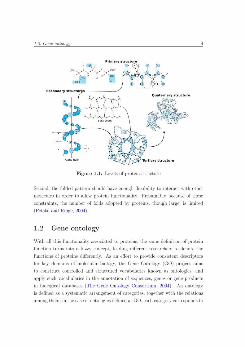
Figure 1.1 depicts the different levels of protein structures.
The secondary structure of the protein can take the form either of alpha helices
or of beta sheets, formed through regular hydrogen-bonding interactions between
molecules in the main amine and carboxyl groups of amino acids, that is, in the
invariant backbone of the chain. In the globular form of the protein, elements of
either alpha helix, or beta sheet, or both, as well as loops and links that have
no secondary structure, are folded into a tertiary structure. Many proteins are
formed by association of the folded chains of more than one polypeptide; this
constitutes the quaternary structure of a protein.
The huge variety of functions that can be performed by proteins comes from
the large number of three dimensional folding patterns resulting from interactions
among the side chains of these amino acids. However, it is important to point out
that there are two constraints for a polypeptide to be a protein. First, it must be
able to form a stable tertiary structure (or fold) under physiological conditions.
1.2. Gene ontology 9
Estructura primaria
Estructurassecundarias
Hélice alfa
Hoja beta
Estructuraterciaria
Estructuracuaternaria
0.54 nm
Primary structure
Secondary structures
Tertiary structure
Quaternary structure
Alpha helix
Beta sheet
Figure 1.1: Levels of protein structure
Second, the folded pattern should have enough flexibility to interact with other
molecules in order to allow protein functionality. Presumably because of these
constraints, the number of folds adopted by proteins, though large, is limited
(Petsko and Ringe, 2004).
1.2 Gene ontology
With all this functionality associated to proteins, the same definition of protein
function turns into a fuzzy concept, leading different researchers to denote the
functions of proteins differently. As an effort to provide consistent descriptors
for key domains of molecular biology, the Gene Ontology (GO) project aims
to construct controlled and structured vocabularies known as ontologies, and
apply such vocabularies in the annotation of sequences, genes or gene products
in biological databases (The Gene Ontology Consortium, 2004). An ontology
is defined as a systematic arrangement of categories, together with the relations
among them; in the case of ontologies defined at GO, each category corresponds to

10 Chapter 1. Preliminary concepts
a functional label or “GO term”, related with other terms through “is-a” or “part-
of” relationships. Structurally, these ontologies could be modeled hierarchically
as directed acyclic graphs, which means that every child node may have more
than one parent node.
There are three ontologies in GO, defined to describe three non-overlapping
domains of molecular biology: molecular function, cellular component and biolog-
ical process. Molecular function (MF) refers to biochemical activities at molecular
level, no matter what entities are in charge of accomplishing that function or the
context where it takes place; examples of molecular functions are “enzyme regula-
tor activity”, “binding activity” or “transport activity”. Cellular component (CC)
refers to the specific sub-cellular location where a gene product is active, describ-
ing different parts of the eukaryotic cell; cellular components include “ribosome”,
“cytoplasm” or “Golgi apparatus”. Biological process (BP) refers to a series of
events or molecular functions, with a defined beginning and end, to which the
gene or gene product contributes; examples are “reproduction”, “protein metabolic
process” or “cell death”.
Bind
MF
NaBind HydrolProtBind
RnaBind
Transf
Catal
NtBind
DnaBind
ChromBind
TranscFact
Motor Nase
SigTransd Receptor
RecBind
StructMol Transp
TranslFact
LipBind
Kinase
OxBind
EnzReg
ChBind
TranslReg
Figure 1.2: Molecular Function ontology from the plants GO-slim. The list ofacronyms can be found in table 2.1
Currently, as of February 2013 there are 38137 defined GO terms, distributed
over 9467 molecular functions, 3050 cellular components and 23928 biological

1.3. Paradigms in machine learning 11
processes. However, it is often useful to have a less detailed set of categories to
produce a high-level overview of functions distribution. For this reason, a number
of custom datasets, named GO slims, are also maintained by The Gene Ontol-
ogy Consortium. In those versions, more specific terms have been collapsed up
into more general parent terms, and they are particularly useful for analyzing
just a subsection of the GO in order to study a particular field or for a gen-
eral genome-wide analysis. In particular, species-specific slims are maintained
for plants (Berardini et al., 2004), Candida Albicans (Costanzo et al., 2006),
Schizosaccharomyces Pombe (Aslett and Wood, 2006) and Saccharomyces Cere-
visiae (Hirschman et al., 2006). As an example, figure 1.2 shows the GO-terms
in the Molecular Function ontology for the plants GO slim.
1.3 Paradigms in machine learning
Machine learning provides the tools for constructing models that represent biolog-
ical knowledge and use it to predict biological outcomes. In particular, this work
is focused on semi-supervised learning methods for predicting protein function-
ality. However, in order to understand the nature of semi-supervised learning, it
will be useful to first define classical supervised and unsupervised learning frame-
works. Then, semi-supervised and semi-unsupervised learning will be properly
defined.
1.3.1 Supervised and unsupervised learning
The field of machine learning has traditionally been divided into two sub-fields:
unsupervised learning and supervised learning. In unsupervised learning, the sys-
tem observes an unlabeled set of items represented by their D-dimensional feature
vectors {xi}Ni=1, xi ∈ RD, drawn from a feature space X. The main objective is
to discover its underlying distribution in order to group them into K clusters. In
this setting, there is no “right” answer, since there is not a prior knowledge about
the correct membership of the samples (which is why this paradigm is termed as
unsupervised).

12 Chapter 1. Preliminary concepts
−20 −10 0 10 20
−4
−2
02
4
x1
x 1
(a) Unclusterd data
−20 −10 0 10 20
−4
−2
02
4
x1
x 1
(b) Clustered data with K=2
−20 −10 0 10 20
−4
−2
02
4
x1
x 1
(c) Clustered data with K=3
Figure 1.3: Example of unsupervised learning
1.3. Paradigms in machine learning 13
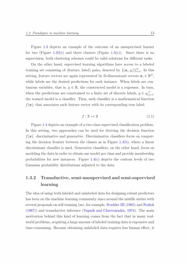
Figure 1.3 depicts an example of the outcome of an unsupervised learner
for two (Figure 1.3(b)) and three clusters (Figure 1.3(c)). Since there is no
supervision, both clustering schemes could be valid solutions for different tasks.
On the other hand, supervised learning algorithms have access to a labeled
training set consisting of (feature, label) pairs, denoted by {(xi, yi)}Ni=1. In this
setting, feature vectors are again represented by D-dimensional vectors xi ∈ RD,
while labels are the desired predictions for each instance. When labels are con-
tinuous variables, that is, y ∈ R, the constructed model is a regressor. In turn,
when the predictions are constrained to a finite set of discrete labels, y ∈ yjCj=1,
the trained model is a classifier. Then, such classifier is a mathematical function
f(x), that associates each feature vector with its corresponding true label:
f : X 7→ Y (1.1)
Figure 1.4 depicts an example of a two-class supervised classification problem.
In this setting, two approaches can be used for deriving the decision function
f(x): discriminative and generative. Discriminative classifiers focus on comput-
ing the decision frontier between the classes as in Figure 1.4(b), where a linear
discriminant classifier is used. Generative classifiers, on the other hand, focus on
modeling the data in order to obtain one model per class and provide membership
probabilities for new instances. Figure 1.4(c) depicts the contour levels of two
Gaussian probability distributions adjusted to the data.
1.3.2 Transductive, semi-unsupervised and semi-supervised
learning
The idea of using both labeled and unlabeled data for designing robust predictors
has been on the machine learning community since around the middle sixties with
several proposals on self-training (see, for example, Scudder III (1965) and Fralick
(1967)) and transductive inference (Vapnik and Chervonenkis, 1974). The main
motivation behind this kind of learning comes from the fact that in many real-
world problems, acquiring a large amount of labeled training data is expensive and
time-consuming. Because obtaining unlabeled data requires less human effort, it

14 Chapter 1. Preliminary concepts
−15 −10 −5 0 5 10 15
−3.
0−
2.5
−2.
0−
1.5
−1.
0−
0.5
0.0
x1
x 1
o
o
o
o
o oo
oo
oo
o
o
o
o
o
o
o
o
o
o
o
oo
o
o
o
o
o
o
o
o
oo
o
o
o
o
o
oo
o
oo
o
oo
oo
o
x
x xx
x
x
x
x
x
x
x
x
x
x xx
x
xxx
x
x
x
x
xx
xxx
x
x
x
x
x
x
xxx
x
x
x
x
x
x
x
x
x
x
x
x
(a) Data
−15 −10 −5 0 5 10 15
−3.
0−
2.5
−2.
0−
1.5
−1.
0−
0.5
0.0
x1
x 1
o
o
o
o
o oo
oo
oo
o
o
o
o
o
o
o
o
o
o
o
oo
o
o
o
o
o
o
o
o
oo
o
o
o
o
o
oo
o
oo
o
oo
oo
o
x
x xx
x
x
x
x
x
x
x
x
x
x xx
x
xxx
x
x
x
x
xx
xxx
x
x
x
x
x
x
xxx
x
x
x
x
x
x
x
x
x
x
x
x
(b) Discriminant classifier
−15 −10 −5 0 5 10 15
−3.
0−
2.5
−2.
0−
1.5
−1.
0−
0.5
0.0
x1
x 1
o
o
o
o
o oo
oo
oo
o
o
o
o
o
o
o
o
o
o
o
oo
o
o
o
o
o
o
o
o
oo
o
o
o
o
o
oo
o
oo
o
oo
oo
o
x
x xx
x
x
x
x
x
x
x
x
x
x xx
x
xxx
x
x
x
x
xx
xxx
x
x
x
x
x
x
xxx
x
x
x
x
x
x
x
x
x
x
x
x
(c) Generative classifier
Figure 1.4: Example of supervised learning

1.3. Paradigms in machine learning 15
is of great interest to include it in the learning process both in theory and in
practice.
There are several ways of combinig those two sources of data, given rise to
different paradigms in machine learning. Consider a system that can observe two
sources of data: the points XL = {xi}Li=1 for which labels {yi}Li=1 are provided,
and the points XU = {xi}L+Ui=L+1 the labels of which are not known. “Transductive”
learning is only interested on predicting the labels of the unlabeled data in the
training dataset, that is, in learning a function of the form:
f : XU 7→ YU (1.2)
here, f is expected to be a good predictor on the unlabeled data and is defined
only on the given training sample, and is not required to make predictions outside.
On the other hand, “inductive semi-supervised” learning is interested on designing
a function able to predict the labels on future test data. That is:
f : X 7→ Y (1.3)
here, f is expected to be a good predictor over the whole feature space and,
implicitly, it is expected to be better than the supervised classifier trained on
the labeled data alone. Like in supervised learning, a common estimation of the
performance of the system with future data can be obtained by using a separate
test sample, which is not available during training. This setting is sometimes
simply called semi-supervised classification and constitutes the main subject of
the present work.
An interesting analogy presented in (Zhu and Goldberg, 2009), proposes that
semi-supervised learning is like an in-class exam, where the questions are not
known in advance, and a student needs to prepare for all possible questions; in
contrast, transductive learning is like a take-home exam, where the student knows
the exam questions and needs not prepare beyond those.
Finally, other forms of partial supervision are also possible. Constrained clus-
tering is an extension to conventional unsupervised clustering which, in addition
to the unlabeled data, is fed with some supervised information about the clus-
ters. Such information is commonly provided in the form of “must-link” and
16 Chapter 1. Preliminary concepts
“cannot link” constraints, imposing restrictions over pairs of instances that must
be or cannot be in the same cluster. Seeger (2006) defines this category of algo-
rithms as “semi-unsupervised learning”, since their main objective is to estimate
the probability distribution of the data as in unsupervised learning methods.
1.3.3 Remarks on the application of machine learning meth-
ods for protein function prediction
Following the notation of (King and Guda, 2008), let P be the protein space (the
set of all possible protein sequences). Labeled data will be noted as PL while
unlabeled data will be noted by PU . Then, we have:
P = PL ∪ PU (1.4)
First, let X be the feature space generated from a characterization function
ζ : P 7→ X. This function accepts as input a protein sequence and returns a
feature vector x ∈ RD, with D physical-chemical and/or statistical attributes of
the protein sequence (this will be explained in more detail in the next chapter).
In general terms, the function ζ is neither injective nor surjective, that means
that several elements in P can be mapped into the same element of X. Besides,
there may be some feature vectors in X for which no instance in P could possibly
exist in nature (King and Guda, 2008).
Let Y be the label set, with all the discrete labels that can be assigned to a
given protein. This set corresponds to all the functional annotations that can
be associated to proteins (the set of GO terms). It is necessary to have into
account that those labels are not mutually exclusive as in traditional supervised
classification, that is, one protein can be associated to more than one GO term
at the same time. Then, each labeled instance will be associated not only to a
single label y but to a set of Q labels that is a subset of the whole set of possible
labels y ⊆ Y.
This gives raise to a multi-label learning problem, a branch of machine learn-
ing where multiple target labels must be assigned to each instance. Multi-label
learning methods can be transformed into one or more single-label classification
problems by employing several topologies Tsoumakas and Katakis (2007). In this

1.4. Single-objective and multi-objective optimization for machine learning methods 17
regard, a recent paper by Giraldo-Forero et al. (2013), empirically demonstrated
that the performance of the “binary relevance” topology, together with a technique
of class balance, remains above several recently proposed techniques for the prob-
lem of predicting protein functions. Binary relevance decomposes the multi-label
decision function f : X 7→ YQ, into Q binary classifiers f q : X 7→ {+1,−1}, where
each binary classifier decides whether or not a given instance should be associated
to the q−th class. This approach is also known as “one against all”, and will be
used for all the experiments in this work. Therefore, the labels will be assumed
to be binary throughout the rest of the document.
Having defined X and Y, it is now possible to apply any machine learning
algorithm (supervised or unsupervised) to the prediction of protein functions.
1.4 Single-objective and multi-objective optimiza-
tion for machine learning methods
The training of most machine learning method comprise of two steps: selecting
a candidate model (that in general terms is a parametric function) and then,
estimating the parameters of the model using an optimization algorithm and
available data. Therefore, all learning problems can be considered as optimization
problems (Jin and Sendhoff, 2008).
For the particular case of protein function prediction, let xi ∈ X be the feature
vector representing the protein pi ∈ P, and let yi ∈ Y be the label assigned to
that element. The predictor function f should satisfy f(xi) = yi, i = 1, 2, . . . , N .
In general terms, this function can belong to a family of parametric functions
with parameters θ:
f ∈ {fθ}θ∈T (1.5)
where T is the space of all the vectors of parameters. Learning the predictor
is achieved by the correct selection of the vector of parameters θ, and such ad-
justment can be understood as an optimization process depending on the labeled
data (for the supervised case) or both the labeled and unlabeled data (for the
semi-supervised case).

18 Chapter 1. Preliminary concepts
Table 1.1: Examples of loss functions and the optimization methods used inseveral supervised machine learning algorithms
Method Loss functionOptimization
algorithm
Least squaresclassifier
(yi − fθ(xi))2 Analytical solution
Multilayerperceptron − (fθ(xi)yi)H (fθ(xi)yi)
†Backpropagation(gradient descent)
Support vectormachine
max(0, 1− yif(xi))Quadratic
programming† H() stands for the Heaviside step function.
In order to perform the estimation of parameters, it is first necessary to define
one or multiple optimization criteria. The most common criterion for supervised
and (inductive) semi-supervised learning is to define an objective function that
reflects the quality of the adjusted model, by minimizing the prediction error over
the training set:
oerr(θ) =
N∑
i=1
ℓ (fθ(xi), yi) (1.6)
where ℓ is some loss function that depends on the desired labels yi and the pre-
dicted labels fθ(xi) of the training set. Table 1.1 shows several examples of the
loss functions used in common machine learning algorithms. The optimization
process must find the optimal vector of parameters θ∗ such that:
θ∗ = argminθ∈T
oerr(θ) (1.7)
However, minimizing the training error is not the only objective to be con-
sidered, since this may result in over-fitting the training data and consequently
obtaining poor performance on unseen data. To avoid this problem, the complex-
ity of the model must be also controlled. This is usually expressed by defining

1.4. Single-objective and multi-objective optimization for machine learning methods 19
another objective fuction in terms of the norm of fθ:
ocomp(θ) = ‖fθ‖ (1.8)
The most common approach for including this new objective in the training
process, is by aggregating the two objectives into a scalar objective function. This
process is known as “regularization”:
θ∗ = argminθ∈T
{oerr(θ) + λocomp(θ)} (1.9)
where λ is a positive scalar constant defined by the user, and the correct deter-
mination of this parameter is not a trivial task. The work by Marler and Arora
(2009) provides an analysis that reveals several fundamental deficiencies of the
scalarization of multi-objective optimization problems, showing that although the
weighted sum method is easy to use, it provides only a linear approximation of
the preference function.
In fact, almost every real-world problem involves simultaneous optimization of
several incommensurable and often competing objectives (Zitzler, 1999). A more
flexible approach to deal with this kind of problems comes from the Pareto-based
optimization strategies. In this setting, the objective function does not provide a
scalar output, but a vector with the evaluation of all the objectives considered:
o(θ) = [o1(θ), o2(θ), . . . , oM(θ)] (1.10)
where M is the number of objectives. It is rarely the case that there is a single
solution that optimizes all the objectives at the same time. Therefore, instead of
a single solution, a set of trade-off solutions must be returned by the optimization
algorithm. Here, it is necessary to modify the notion of optimality. The most
commonly adopted notion is the generalized by Pareto (1896), called “Pareto
optimality”. in a minimization multi-objective problem, a solution θ∗ is said to
be Pareto-optimal if there is no other feasible solution θ ∈ T which would decrease
one of the objective functions without causing a simultaneous increase in at least
one other objective function. A formal definition can be established by first
20 Chapter 1. Preliminary concepts
0 1 2 3 4
0.0
0.5
1.0
1.5
2.0
o1 = ∑i=1
2θi
2
o 2=
∑ i=12(θ
i−0.
5)2
Dominated objectivesPareto front
(a) Objective functions space
−1.0 −0.5 0.0 0.5 1.0
−1.
0−
0.5
0.0
0.5
1.0
θ1θ 2
Dominated solutionsNon−dominated solutions
(b) Search space
Figure 1.5: Example of a Pareto front
defining the notion of Pareto-dominance (Zitzler, 1999) between two solutions θ
and φ:
θ � φ (θ weakly dominates φ) ⇐⇒ ∀i ∈ {1, 2, . . . ,M} : oi(θ) ≤ oi(φ) (1.11)
θ ≺ φ (θ dominates φ) ⇐⇒ θ � φ ∧ o(θ) 6= o(φ) (1.12)
then, a solution θ∗ is said to be Pareto-optimal if and only if:
∄θ ∈ T : θ ≺ θ∗ (1.13)
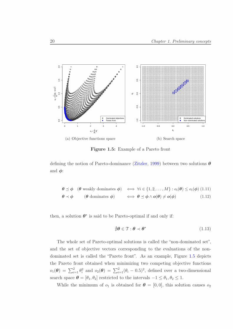
The whole set of Pareto-optimal solutions is called the “non-dominated set”,
and the set of objective vectors corresponding to the evaluations of the non-
dominated set is called the “Pareto front”. As an example, Figure 1.5 depicts
the Pareto front obtained when minimizing two competing objective functions
o1(θ) =∑2
i=1 θ2i and o2(θ) =
∑2i=1(θi − 0.5)2, defined over a two-dimensional
search space θ = [θ1, θ2] restricted to the intervals −1 ≤ θ1, θ2 ≤ 1.
While the minimum of o1 is obtained for θ = [0, 0], this solution causes o2
1.4. Single-objective and multi-objective optimization for machine learning methods 21
to produce an output of 0.5. In turn, the minimum value of o2 is reached for
θ = [0.5, 0.5], causing o1 to produce an output of 0.5. These two points correspond
to the ends of the Pareto font in Figure 1.5(a), while all the intermediate points
lying on the Pareto front are also good trade-off solutions for the multi-objective
problem: in the absence of preference information, none of the corresponding
trade-offs can be said to be better than the others. Figure 1.5(b), depicts the
location of the non-dominated solutions in the original search space.


Chapter 2
Supervised Gene Ontology
prediction for Embryophyta
organisms
Currently, there are almost 8 million sequences in non-redundant databases, in-
cluding the complete genomes of ≈ 1, 800 different species. However, for most of
them, we know just their primary structure: the linear amino acid sequence de-
duced from the DNA chain (Levitt, 2009). Assessment of protein functions needs
in most cases of experimental approaches carried out in the lab. Such approaches
require either cloned DNA or protein samples from the genes of interest. Ex-
perimental procedures for probing protein function includes DNA micro-arrays
for providing expression patterns of genes; two dimensional gel electrophoresis
which can separate complex protein mixtures into their components for being
identified by mass spectrometry; gene knockout experiments for studying phe-
notypical effects of inactivating determined gene products and experiments with
green fluorescent protein for determining gene products locations.
Unfortunately, this procedures must be usually focused on specific proteins or
functions, and the current dimensions of data bases makes of manual annotation
a difficult and almost intractable problem. Additionally, experimental determi-
nation of the function of many proteins is very likely to be hard, because the
function may be related specifically to the native environment in which a par-

24 Chapter 2. Supervised Gene Ontology prediction for Embryophyta organisms
ticular organism lives. Such perspective has lead some authors to conclude that
the only effective route toward the elucidation of the function of some proteins
may be computational analysis and prediction from amino acid sequences, obtain-
ing a first hint toward functionality that later can be subjected to experimental
verification (Baldi and Brunak, 2001, chapter 1).
2.1 Gene Ontology predictors
Many approaches have been developed in this matter (for full surveys, see (Fried-
berg, 2006; Pandey et al., 2006; Zhao et al., 2008c)). One of the earliest appli-
cations, yet still one of the more popular bioinformatics tools is the Basic Local
Alignment Search Tool for proteins (BLASTP) (Altschul et al., 1997) which has
been applied for obtaining annotation transfers based on sequence alignments.
Also, a high number of methods (GOblet (Groth et al., 2004), OntoBlast (Ze-
hetner, 2003), GOFigure (Khan, 2003) and GOtcha (Martin et al., 2004)) are
based on the idea of refining and improving initial results from classic align-
ment tools such as BLASTp, by performing mappings and weightings of GO
terms associated to BLASTP predictions. However, in such methods, the fail-
ure of conventional alignment tools to adequately identify homologous proteins
at significant E-values is not considered (Hawkins et al., 2009). The same ap-
plies for some more recent methods that have improved specific points of this
methodology such as speeding up the procedure through decision rules ((Jones
et al., 2008)), including additional functionality for visualization and data mining
((Conesa and Götz, 2008)) or also including some statistics of GO terms to refine
selection ((Vinayagam et al., 2006)). In order to avoid the dependency to BLAST
alignments in the cases where the alignment-based annotation transfer approach
is not so effective, more recent methods have used machine learning techniques
trained over feature spaces of physical-chemical, statistical or locally-based at-
tributes. Those methods employ techniques such as neural networks (ProtFun
(Jensen et al., 2003)), Bayesian multi-label classifiers ((Jung and Thon, 2008))
and support vector machines (SVM-Prot (Cai, 2003), GOKey (Bi et al., 2007),
PoGO (Jung et al., 2010)), obtaining high performance results in their own re-
2.1. Gene Ontology predictors 25
spective databases, mostly composed by model organisms such as bacteria and a
few high order species.
There are, however, several aspects that must be discussed about current
performance in prediction of GO terms, when applied to non-model organisms
such as land plants (Embryophyta). First, from the previously described methods,
only Blast2GO (Conesa and Götz, 2008) was specialized for predicting GO terms
in plant proteins. In fact, as it is pointed out by the authors of Blast2GO, very few
resources are available for large-scale functional annotation of non-model species.
Some methods specialized on vegetative species have been proposed recently, but
they are only intended for performing cellular component predictions (Predotar
(Small et al., 2004), TargetP (Emanuelsson et al., 2000), Plant-mPloc (Chou
and Shen, 2010)). Moreover, Predotar and TargetP can discriminate among only
three or four cellular location sites. Plant-mPloc, in turn, covers twelve different
location sites and it was rigorously tested over a set of proteins with less than
25% of identity among them, where homologue-based tools like BLASTP would
certainly fail. For such dataset, they obtained an overall success rate of 63.7%,
much less than reported by other cellular location predictors tested over non-plant
datasets. Second, none of the existing methods can be used to deal with plant
proteins that can simultaneously exist or move between two or more different
location sites (Chou and Shen, 2010), or belong to multiple functional classes at
the same time (Briesemeister et al., 2010).
In order to improve the performance of current GO term predictors for land
plants, it would be useful to have a better understanding of the underlying rela-
tionships between primary structure information and protein functionality. How-
ever, the structure of the machine learning models behind high-accuracy predic-
tors often makes difficult to understand why a particular prediction was made
(Briesemeister et al., 2010). In this sense, a recent method called Yloc (Briese-
meister et al., 2010) was proposed for analyzing what specific features are respon-
sible for given predictions. This method, nevertheless, is not intended to predict
GO terms, but instead, it uses annotation information from PROSITE (Sigrist
et al., 2010) and GO as inputs to the predictor. Additionally, their study is only
focused on predicting protein locations in the cell.

26 Chapter 2. Supervised Gene Ontology prediction for Embryophyta organisms
Since most of the current GO prediction methods are limited to a few arbi-
trary functional classes and single ontologies, they cannot provide any information
about relationships on the predictability at the various levels of protein function-
ality (molecular, cellular, biological), which could be another key element for
determining how the information of the primary structure is related to protein
function.
2.2 Proposed methodology: prediction of GO terms
in Embryophyta organisms with pattern recog-
nition techniques
This section presents an analysis on the predictability of GO terms over the
Embryophyta group of organisms, which is composed by the most familiar group
of plants including trees, flowers, ferns, mosses, and various other green land
plants. The analysis provides the following key elements: predictions are made
by using features extracted solely from primary structure information; analysis
comprises most of the available organisms belonging to the Embryophyta group;
biases due to protein families are avoided by considering only proteins with low
similarity among them and a strong evidence of existence; predictions and analysis
are made over a set of categories belonging to the three ontologies; proteins are
allowed to be associated to several GO terms simultaneously.
Results from this chapter answer whether it is possible to predict most GO-
slim terms from primary structure information, what categories are more suscep-
tible to be predicted, which ontology is most related to the information contained
in the primary structure and what relationships among ontologies could be influ-
encing the predictability at different levels of protein functionality in land plants.
The implemented methodology for assessing predictability of GO terms in
Embryophyta proteins comprises the following parts: (i) selection of the pro-
tein sequences conforming the database in order to cover the highest number of
available plant proteins, while ensuring high confidence annotations and avoiding
possible biases; (ii) categories describing positive and negative samples associated
to each GO term are determined in order to minimize the impact of hierarchical

2.2. Proposed methodology: prediction of GO terms in Embryophyta organisms with
pattern recognition techniques 27
relationships; (ii) protein sequences are mapped into feature vectors that encode
a number of attributes of varied nature; (iii) computed features are clustered into
groups of similar information content; (iv) one binary classifier is learned for each
GO term and each feature cluster in order to evaluate the prediction power of
individual clusters, and finally (v) one binary classifier is learned for each GO
term using the whole set of features in conjunction with an automatic feature se-
lection strategy in order to determine the global predictability of each GO term.
The following subsections describe the methods employed for each part of the
methodology.
2.2.1 Database
The database comprises all the available Embryophyta proteins at UniProtKB/Swiss-
Prot database (Jain et al., 2009, file version: 10/01/2013), with at least one an-
notation in the Gene Ontology Annotation (GOA) project (Barrell et al., 2008,
file version: 7/01/2013). The resulting set comprises proteins from 189 different
land plants.
In order to avoid the presence of protein families that could bias the results,
the dataset was filtered at several levels of sequence identity using the Cd-Hit
software (Li and Godzik, 2006). The main results are reported for the lowest
identity cutoff (30%). However, additional analyses at 40%, 50%, 60%, 70% and
80% were also performed in order to provide further information on the robustness
of the method. It is important to mention that, according to (Petsko and Ringe,
2004)[chapter 4], function can be inferred from homology based transfer methods
in cases where a protein has more than about 40% sequence identity to another
protein whose biochemical function is known, and if the functionally important
residues are conserved between the two sequences. Identities under 40% do not
allow to make function prediction with high confidence when using the classical
methods.
The main set comprises a total of 3368 protein sequences, from which 1973
sequences are annotated with molecular functions, 2210 with cellular compo-
nents and 2798 with biological processes. Finally, it is also important to clar-
ify that, although computational and indirectly derived annotations increase

28 Chapter 2. Supervised Gene Ontology prediction for Embryophyta organisms
coverage significantly, they probably contain a higher portion of false positives
(Rhee et al., 2008). Consequently, annotations associated to evidence codes from
automatically-assigned annotations were not included in the analyses.
2.2.2 Definition of classes
Although, in principle, the method can be trained to predict any GO term for
which there are enough training sequences, all tests were performed over the
set of categories defined by the plants GO slim developed by The Arabidopsis
Information Resource - TAIR (Berardini et al., 2004, file version: 14/03/2012).
This choice was made because GO includes a large number of categories that
do not occur in plants, due to its broad size. In turn, slims are smaller, more-
manageable sub-sets of GO, that focus on terms relevant to a specific problem
or data set (Davis et al., 2010), thus allowing to generate higher-level annotation
more robust to tests of statistical significance (Rhee et al., 2008).
Positive and negative samples associated to each GO term are selected by
considering the propagation principle of GO in order to avoid hierarchical rela-
tionships. Otherwise, as members of child categories are also included on parent
categories, classes would be totally overlapped and no standard classification tool
could be successful. If a protein is predicted to be associated to any given GO
term, it must be automatically associated to all the ancestors of that category
and thus, it is enough to predict only the lowest level entries. Consequently, for
each GO term, positive samples are all those proteins that have been annotated
with this term or any of its descendants, excepting those descendants that are also
included as categories. All the remaining samples in the database are selected
as negative samples for that GO term. It is very important to keep in mind the
interpretability implications of this procedure, in order to correctly understand
posterior results. As said before, GO slims are reduced versions of GO, where
more specific terms have been collapsed up into parent terms. For instance, the
term “nucleic acid binding” has five children in the original GO molecular func-
tion ontology, while it only has three children in the plants GO slim, what means
that the remaining two children were merged up into the parent. After removing
2.2. Proposed methodology: prediction of GO terms in Embryophyta organisms with
pattern recognition techniques 29
redundant entries, sequences remaining in “nucleic acid binding” category are pre-
cisely the ones associated to that two merged categories, as well as to every other
function not explicitly listed in GO. For that reason, a correct interpretation of
this category should be now “other members of nucleic acid binding”, clarifying
the disruption with the three explicit children. For avoiding possible confusions,
redefined classes are marked with an asterisk throughout the document.
After defining the membership of the sequences, categories with less than 30
proteins were discarded because they did not have enough samples to train a
statistically reliable classifier. The final set is thus comprised by 14 GO terms in
the molecular function ontology, 20 GO terms in the cellular component ontology
and 41 GO terms in the biological process ontology. Table 2.1 shows the final list
of categories, as well as the acronyms used to cite them throughout this paper
and the number of samples in each one for the 30% identity cutoff.
2.2.3 Characterization of protein sequences
Protein sequences were mapped into feature vectors by extracting three types of
attributes: physical-chemical features, primary structure composition statistics
and secondary structure composition statistics (see Table 2.2).
The first group is intended to provide information directly related with bio-
chemistry of the molecule and is constituted by six properties related to basic
physical-chemical attributes of amino acids. Weight of the sequence is influenced
by the size of the constituent amino acids; polarity of amino acid side chains
determines the percentage of positively and negatively charged residues in the
sequence; acidic or basic nature of amino acids determines the isoelectric point
of the sequence and grand average of hydropaticity index (GRAVY) measures
whether the protein is hydrophobic (positive GRAVY) or hydrophilic (negative
GRAVY).
The second group of features is based on the increasing use of document classi-
fication techniques for protein sequence classification (Cheng et al., 2005; Ganap-
athiraju et al., 2005), where characterization is done by counting the occurrences
of all possible subsequences of a fixed length n, called n-grams or n-mers, over
the primary structure of the protein. In this work, only features corresponding

30 Chapter 2. Supervised Gene Ontology prediction for Embryophyta organisms
Table 2.1: Definition and size of the classes. The list of GO terms covered bythis analysis is intended to provide a complete landscape of GO predictability atthe three levels of protein functionality in Embryophyta plants. For classificationpurposes, classes marked with an asterisk (*) were redefined. The number ofsamples in those categories corresponds to the sequences associated to that classand none of its also listed descendants.
Class Acronym Size Class Acronym Size
Molecular Function Biological Process
Nucleotide binding Ntbind 47 Reproduction* Reprod* 337
Molecular function* MF* 268 Carbohydrate metabolic process ChMet 315
DNA binding DnaBind 107 Generation of precursor metabolitesMetEn 150
Transcription factor activity TranscFact 307 and energyRNA binding RnaBind 43 Nucleobase, nucleoside, nucleotide,
NaMet* 712Catalytic activity* Catal* 334 nucleic acid metabolic process*Receptor binding RecBind 38 DNA metabolic process DnaMet 191
Transporter activity Transp 125 Translation Transl 82
Binding* Bind* 173 Protein modification process ProtMod 391
Protein binding* ProtBind* 630 Lipid metabolic process LipMet 324
Kinase activity Kinase 68 Transport Transport 531
Transferase activity* Transf* 173 Response to stress StressResp 790
Hydrolase activity Hydrol 190 Cell cycle CellCycle 234
Enzyme regulator activity EnzReg 41 Cell communication* CellComm* 66
Signal transduction SigTransd 305
Cell-cell signaling Cell-cell 53
Cellular Component Multicellular organismal development* MultDev* 490
Cellular component* CC* 234 Biological process* BP* 879
Extracellular region ExtcellReg 109 Metabolic process* Met* 279
Cell wall CellWall 77 Cell death CellDeath 95
Intracellular* Intracell* 167 Catabolic process Catabolic 479
Nucleus* Nucleus* 421 Biosynthetic process* Biosint* 1125
Nucleoplasm NuclPlasm 51 Response to external stimulus* ExtResp* 65
Nucleolus Nucleolus 84 Tropism Tropism 36
Cytoplasm* CitPlasm* 168 Response to biotic stimulus BioResp 275
Mitochondrion Mitochond 244 Response to abiotic stimulus AbioResp 642
Endosome Endosome 58 Anatomical structure morphogenesis StrMorph 366
Vacuole Vacuole 171 Response to endogenous stimulus EndoResp 332
Peroxisome Peroxisome 32 Embryonic development EmbDev 139
Endoplasmatic reticulum EndRet 109 Post-embryonic development* PostDev* 375
Golgi apparatus GolgiApp 100 Pollination Poll 43
Cytosol Cytosol 389 Flower development FlowerDev 228
Ribosome Ribosome 98 Cellular process* CP* 1486
Plasma membrane PlasmMb 353 Response to extracellular stimulus ExtcellResp 59
Plastid Plastid 696 Photosyntesis Photosyn 102
Thylakoid Thylk 147 Cellular component organization CellOrg 757
Membrane* Mb* 472 Cell growth CellGrowth 133
Protein metabolic process* ProtMet* 187
Cellular homeostasis CellHom 53
Secondary metabolic process SecMet 164
Cell differentiation CellDiff 267
Growth* Growth* 64
Regulation of gene expression,RGE 103
epigenetic

2.2. Proposed methodology: prediction of GO terms in Embryophyta organisms with
pattern recognition techniques 31
Table 2.2: Initial set of features extracted from amino acid sequences. Fea-tures are divided into three broad categories: physical-chemical features, primarystructure composition statistics and secondary structure composition statistics.
Nature Description Number
Physical-chemical
Sequence length 1Molecular weight 1Positively charged residues (%) 1Negatively charged residues (%) 1Isoelectric point 1GRAVY 1
Primary structure statisticsAmino acid frequencies 20Amino acid dimer frequencies 400
Secondary structure statisticsStructure frequencies 3Structural dimer frequencies 9
Total 438
to n = {1, 2} are employed, provided that the size of the feature space grows
exponentially with n. Simple countings were converted to relative frequencies
(summing to one) in order to obtain information relative to the sequence compo-
sition more than simple presence statistics.
The third group is analog to the second one, but applying the n-gram charac-
terization to the predicted secondary structure of the protein. Predictions were
calculated by employing the Predator 2.1 software (Frishman and Argos, 1997),
whose output is a linear sequence with three structural domains: alpha helices,
beta sheets and coils. It is worthy to note that even though this group of features
were computed over secondary structure information, they must be still consid-
ered as derived from primary structure because there is no full certainty about
correctness of the secondary structure prediction.
It is important to point out that in the case of ambiguity characters in the se-
quence, that is, characters used to denote lack of information at certain positions
(B for asparagine or aspartic acid, J for isoleucine or leucine, Z for glutamine or
glutamic acid, X for any amino acid), each feature was computed as its statistical
expected value with natural abundance percentages of amino acids as their prior
probabilities (Buxbaum, 2007, chapter 1). Additionally, since different groups of
features are very heterogeneously scaled (for instance, sequence length is ranged
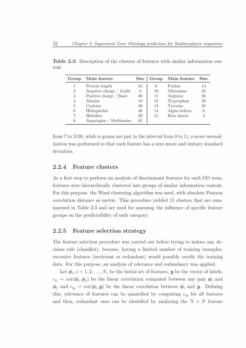
32 Chapter 2. Supervised Gene Ontology prediction for Embryophyta organisms
Table 2.3: Description of the clusters of features with similar information con-tent
Group Main feature Size Group Main feature Size
1 Protein length 34 9 Proline 142 Negative charge / Acidic 8 10 Glutamine 353 Positive charge / Basic 30 11 Arginine 264 Alanine 10 12 Tryptophan 385 Cysteine 38 13 Tyrosine 356 Hidrophobic 46 14 Alpha helices 67 Histidine 29 15 Beta sheets 48 Asparagine / Methionine 85
from 7 to 5138, while n-grams are just in the interval from 0 to 1), z-score normal-
ization was performed so that each feature has a zero mean and unitary standard
deviation.
2.2.4 Feature clusters
As a first step to perform an analysis of discriminant features for each GO term,
features were hierarchically clustered into groups of similar information content.
For this purpose, the Ward clustering algorithm was used, with absolute Pearson
correlation distance as metric. This procedure yielded 15 clusters that are sum-
marized in Table 2.3 and are used for assessing the influence of specific feature
groups on the predictability of each category.
2.2.5 Feature selection strategy
The feature selection procedure was carried out before trying to induce any de-
cision rule (classifier), because, having a limited number of training examples,
excessive features (irrelevant or redundant) would possibly overfit the training
data. For this purpose, an analysis of relevance and redundancy was applied.
Let φi, i = 1, 2, . . . , N , be the initial set of features, y be the vector of labels,
cij = cor(φi,φj) be the linear correlation computed between any pair φi and
φj and ciy = cor(φi,y) be the linear correlation between φi and y. Defining
this, relevance of features can be quantified by computing ciy for all features
and then, redundant ones can be identified by analyzing the N × N feature

2.2. Proposed methodology: prediction of GO terms in Embryophyta organisms with
pattern recognition techniques 33
correlation matrix. In order to speed up the calculus, an algorithm based on the
Fast Correlation-Based Filter of (Yu and Liu, 2004) was used.
First, an initial feature subset is selected based on a predefined threshold on
ciy. Then, the concept of approximate Markov blanket is used to select predomi-
nant features from this relevant set. As defined by (Yu and Liu, 2004), the feature
φi forms an approximate Markov blanket for φj, (i 6= j) if and only if ciy ≥ cjy
and cij ≥ cjy. This principle states that if the information shared between any
pair of features is less or equal than information shared between one of them and
the class labels, the one with lesser information could be discarded. Since the
feature with highest correlation with the class labels does not have any approxi-
mate Markov blanket, it must be one of the predominant features and is taken as
reference. The algorithm proceeds to compute correlation between the reference
and all the remaining features by decreasing order of relevance; if the reference
happens to form an approximate Markov blanket for some feature φi, the last is
removed from the relevant features set. After one round of filtering features based
on the first relevant one, the algorithm will take the remaining feature right next
to it as the new reference to repeat the filtering process. The algorithm stops
when no more predominant features can be selected.
2.2.6 Decision making
Support vector machines (SVM) were chosen as base classifiers for running all
the supervised tests. SVMs are powerful tools for solving classification problems,
designed over a strong theoretical background based on the idea of minimizing
the structural risk (Vapnik, 1998). For a linear SVM, the objective is to find a
classification function of the form:
f(w,b)(x) = 〈w,x〉+ b (2.1)
where 〈·, ·〉 represents the dot product. Following the notation in section 1.4, a
vector of parameters can be defined as θ = [w, b], and the optimization problem

34 Chapter 2. Supervised Gene Ontology prediction for Embryophyta organisms
can be stated as follows:
θ∗ = argminθ∈T
{1
2||θ||2 + C
L∑
i=1
ℓ (fθ(xi)yi)
}(2.2)
where ℓ(t) = max(0, 1−t) is the hinge loss function and C is a trade-off parameter
regulating the complexity of the model. For the non-linear case, the data are first
mapped in a high dimensional Hilbert space H through a mapping Φ : X 7→ H,
and then a linear decision boundary is constructed in that space. The mapping Φ
can be explicitly computed or only implicitly through the use of a kernel function
K such that K(x1,x2) = 〈Φ(x1),Φ(x2)〉. The Representer Theorem can be used
to show that the solution function has the form:
fθ∗(x) =L∑
i=1
αiK(x,xi) (2.3)
where the coefficients αi can be found with a conventional quadratic optimiza-
tion algorithm. The Gaussian kernel is the most commonly used because of its
attractive features such as structure preservation (Liu et al., 2012). This kernel
is computed by:
K(x1,x2) = e−‖x1−x2‖
2σ
2
(2.4)
where σ is the dispersion parameter that must be properly chosen by the user. In
this work, the SVM is trained with the ’kernlab’ package, available in R-CRAN
(Karatzoglou et al., 2004). Dispersion of the kernel and trade-off penalization
parameter of the SVM are tuned for each test with a particle swarm optimization
meta-heuristic, a bio-inspired optimization method that has been used in multiple
applications in the past years (Kennedy and Eberhart, 1995).
In order to allow samples to be associated to multiple categories, decision
making was implemented following the one-against-all strategy. The method
produced a strong class imbalance since it trains a number of binary classifiers,
each one intended to recognize samples from one class out of the whole training
set. In other words, since all the proteins outside of the target GO term are
seen as negative samples and there are only a relatively small number of proteins

2.3. Results and Discussion 35
annotated with the function, the number of negative samples may be hundreds
and even thousands times the one of positive samples. Therefore, the classifier
may be degraded by the false negative samples or imbalanced data (Zhao et al.,
2008d). To overcome the problems that imbalanced classes commonly produce in
pattern recognition techniques, the Synthetic Minority Over-sampling Technique
(SMOTE) was employed (Chawla et al., 2002).
In order to estimate the performance of the predictive model, a 5-fold cross-
validation strategy is implemented. In such strategy, the test procedure is re-
peated five times, and each time an 80% of the data is used for adjusting the
SVM parameters and training the model, while the remaining 20% is used as
testing samples. This strategy also allows providing an estimation of the relia-
bility of the model by computing the variability of the results through the five
repetitions.
2.3 Results and Discussion
2.3.1 Analysis of predictability with individual feature clus-
ters
Classification results with individual feature clusters, for an identity cutoff of 30%,
are condensed in Figure 2.1. The square root of the product between sensitivity
and specificity (geometric mean), is depicted as global performance measure and
the color scale has been adjusted to highlight the highest (green) and the lowest
(blue) performance. Note that the rows and columns have been ordered to ex-
plicitly locate best predicted GO terms on top and most discriminant groups to
the left.
Figure 2.1(a) shows the analysis for the molecular function ontology. For
all feature groups, Receptor binding achieved the highest classification scores.
This category is intended to comprise proteins that interact selectively and non-
covalently with one or more specific sites on a receptor molecule. About 63%
of the proteins associated to this category in the database are proteins involved
with binding of serine/threonine kinase receptors, which turned out to be easily
predicted from most of the defined features.

36 Chapter 2. Supervised Gene Ontology prediction for Embryophyta organisms
3 1 6 15 8 7 2 14 10 4 11 13 5 12 9
MF*
Bind*
EnzReg
RnaBind
NtBind
Catal*
ProtBind*
Hydrol
Transf*
DnaBind
Kinase
Transp
TranscFact
RecBind
Feature sets
(a) Molecular function
1 3 6 9 8 2 11 14 10 4 7 5 15 13 12
CC*
Mb*
Mitochond
Perixosome
Endosome
Vacuole
PlasmMb
Intracell*
Plastid
Cytosol
CellWall
GolgiApp
EndRet
CytPlasm*
ExtcellReg
NuclPlasm
Nucleolus
Thylk
Nucleus*
Ribosome
Feature sets
(b) Cellular component
1 6 8 4 3 9 10 11 13 7 15 5 2 12 14
BP*StressRespExtcellResp
Met*CP*
CellComm*Growth*
CellDeathBioResp
PollProtMet*
CellDiffTransport
ChMetBiosint*
EndoRespCellGrowth
TranslCatabolicAbioResp
LipMetCellHom
StrMorphSigTransd
CellOrgSecMet
EmbDevExtResp*PostDev*
MetEnNaMet*
ProtModReprod*
MultDev*FlowerDev
PhotosynCell−cellDnaMet
CellCycleTropism
RGE
Feature sets
< 0.2
0.3
0.4
0.5
0.6
0.7
> 0.8
Per
form
ance
(G
eom
etric
mea
n)
(c) Biological process
Figure 2.1: Prediction performance with different feature clusters. Rows repre-sent classes in Table 2.1 while columns represent feature groups in Table 2.3. Foreach ontology, best predicted categories are ordered from top to bottom whilemost discriminant feature groups are ordered from left to right.
2.3. Results and Discussion 37
Transcription factor activity achieved was easily predicted from the feature
groups 1, 3, 6, 8 and 14. Not so surprising is the fact that DNA binding also
presents a similar behavior since most transcription factors must interact with
DNA molecules and consequently they are also included in this category. However
it is worthy to note that several other proteins also perform DNA cleavage, such
as polymerases, nucleases and histones, and they were also well predicted from the
same feature groups. The conclusion from these results becomes more evident
by observing the results of the DNA metabolic process in Figure 2.1(c), which
confirm the high predictability of all proteins involved with transcription when
using the mentioned features groups. A similar behavior is also observed for
nucleus* in Figure 2.1(b), supported by the fact that the transcription process is
mostly carried out in that sub-cellular location.
Transporter activity refers to proteins that enable the directed movement of
substances into, out of, within or between cells. Most of them are integral trans-
membrane proteins, that are distinguished by their high content of hydrophobic
residues (Whitford, 2005). In fact, some of the highest performance of transporter
activity were reached with the groups 3 and 6, which include GRAVY index as
well as monomer and dimer frequencies of three out of the four most hydropho-
bic residues: leucine, isoleucine and phenylalanine. Additionally, predictability
of this molecular function is reflected, while in a minor degree, on the transport
biological process, which reaches its highest values for the same feature groups
(see Figure 2.1(c)). The main difference between those GO terms lies in that
transport is a broader category, including external agents such as oxygen carriers
and lipoproteins that perform transport within multicellular organisms.
On the other hand, the root node of the molecular function ontology was
GO terms with the lowest average prediction performance. Remember that the
root node contains the proteins that do not belong to any of its descendant
categories, so it keeps a small set of sequences of a sparse nature, which explains
the impossibility to model and predict them as a group. It is interesting to note
that the same behavior is observer for the other two ontologies (figures 2.1(b)
and 2.1(c)).
Concerning the cellular component ontology, it can be observed in Figure
2.1(b) that ribosome category has reached the highest classification accuracies,

38 Chapter 2. Supervised Gene Ontology prediction for Embryophyta organisms
specially with groups 1, 2, 3 and 11. Such groups mainly consist of the four
charged residues: lysine, arginine, glutamic acid and aspartic acid. This can
be explained since ribosomal proteins must interact with the negatively charged
phosphodiester bonds in the RNA backbone, so they are expected to have a
high percentage of positively charged residues to neutralize such charge repulsion.
In agreement with this, (Whitford, 2005) describes the composition of isolated
ribosomal proteins as showing a high percentage of lysine and arginine residues
and a low aromatic content. Hence, there is enough evidence to establish that
ribosomal proteins are another highly predictable category from primary structure
information.
As explained before, nucleus* becomes easily predicted from the same fea-
ture groups that have shown high discriminant capabilities for transcription re-
lated proteins. A similar behavior is also observed for proteins belonging to the
nucleolus component, which encompasses proteins including RNA polymerases,
transcription factors, processing enzymes and ribosomal proteins among others,
which must interact with nucleic acids and have shown low isoelectric points in
comparison to the remaining proteins in the database.
Thylakoid proteins also presented high prediction performance with several
feature groups. Further studies would be required to explain this results.
Broad categories such as membrane* showed poor performance with most
feature groups, presumably due to its high diversity. However, some rather well-
defined categories such as mitochondrion and perixosome were also ranked in the
lowest places in figure 2.1(b), simply proving to be poorly predictable from the
extracted feature groups.
Concerning figure 2.1(c), the biological process that was better predicted for
most group features is regulation of gene expression, epigenetic. This GO term
encloses proteins involved in modulating the frequency, rate or extent of gene
expression and is highly composed by histones. In fact, since histones are highly
alkaline proteins, it is consistent to observe that this category became particularly
well predicted from groups 3, 6 and 7, which are mainly conformed by frequencies
of phenylalanine, leucine, isoleucine, lysine and histidine residues. Also, cysteine
related frequencies were highly discriminant for regulation of gene expression,
epigenetic (group 5 which can be explained by the fact that altering the redox

2.3. Results and Discussion 39
state of cysteines serves for modulating protein activity, and several transcription
factors become activated by the oxidation of cysteines that form disulfide bonds
(Arrigo, 1999).
Tropism and Cell Cycle also appeared near the top of figure 2.1(c), just before
DNA metabolic process which was already discussed.
2.3.2 Analysis of predictability with the full set of features
Analyses in the previous section were done after discarding sequences with iden-
tities superior to 30%. Otherwise, the predictability of certain terms could be
enhanced from the fact that many proteins in training and testing sets are copies
(or close relatives) from another, rather than from predictive value of certain
sequence-derived features. However, in order to provide further information on
the robustness of the proposed methodology when the identity cutoff changes,
Figure 2.2 presents an analysis of predictability with the full feature set (al-
though applying the feature selection procedure described in the methods sec-
tion), while varying the identity cutoff. For comparison purposes, results achieved
by BLASTP are depicted in blue, while results of the proposed methodology are
depicted in green. The first thing that can be noted from Figure 2.2 is the fact
that alignment-based predictions are more sensitive to the variation of the identity
percentage than the proposed methodology. It can be clearly seen that BLASTP
suffers a strong performance degradation as the identity filter is more stringent,
while the performance of the proposed methodology remains more stable. More-
over, although in Figure 2.2(a) it can be seen that, when predicting molecular
functions, BLASTP is superior than the proposed methodology for high iden-
tity cutoffs, the difference at 30% is not statistically significant. Conversely, the
proposed methodology clearly outperforms BLASTP for low identity percentages
when predicting cellular components and biological processes (figures 2.2(b) and
2.2(c)).
Figure 2.3 depicts detailed results of predicting each class with the full feature
set for an identity cutoff of 30%. Left plots show sensitivity, specificity and geo-
metric mean (green line) achieved with the five-fold cross-validation procedure, as
well as the performance of the BLASTP algorithm for comparison purposes (blue

40 Chapter 2. Supervised Gene Ontology prediction for Embryophyta organisms
Identity percentage
Geom
etr
ic m
ean
30 40 50 60 70 80
0.4
0.5
0.6
0.7
0.8
0.9
SVM
BLASTp
(a) Molecular function
Identity percentage
Geom
etr
ic m
ean
30 40 50 60 70 80
0.2
0.3
0.4
0.5
0.6
0.7
0.8
SVM
BLASTp
(b) Cellular component
Identity percentage
Geom
etr
ic m
ean
30 40 50 60 70 80
0.1
0.2
0.3
0.4
0.5
0.6
0.7
0.8
SVM
BLASTp
(c) Biological process
Figure 2.2: Performance variation in function of the identity cutoff. Green andblue plots show the variation of the general prediction performance for SVM andBLASTP, respectively, according to the identity percentage cutoff used in thedataset. Boxplots show the dispersion throughout the 75 GO terms.
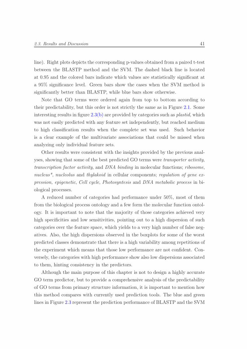
2.3. Results and Discussion 41
line). Right plots depicts the corresponding p-values obtained from a paired t-test
between the BLASTP method and the SVM. The dashed black line is located
at 0.95 and the colored bars indicate which values are statistically significant at
a 95% significance level. Green bars show the cases when the SVM method is
significantly better than BLASTP, while blue bars show otherwise.
Note that GO terms were ordered again from top to bottom according to
their predictability, but this order is not strictly the same as in Figure 2.1. Some
interesting results in figure 2.3(b) are provided by categories such as plastid, which
was not easily predicted with any feature set independently, but reached medium
to high classification results when the complete set was used. Such behavior
is a clear example of the multivariate associations that could be missed when
analyzing only individual feature sets.
Other results were consistent with the insights provided by the previous anal-
yses, showing that some of the best predicted GO terms were transporter activity,
transcription factor activity, and DNA binding in molecular functions; ribosome,
nucleus*, nucleolus and thylakoid in cellular components; regulation of gene ex-
pression, epigenetic, Cell cycle, Photosyntesis and DNA metabolic process in bi-
ological processes.
A reduced number of categories had performance under 50%, most of them
from the biological process ontology and a few form the molecular function ontol-
ogy. It is important to note that the majority of those categories achieved very
high specificities and low sensitivities, pointing out to a high dispersion of such
categories over the feature space, which yields to a very high number of false neg-
atives. Also, the high dispersions observed in the boxplots for some of the worst
predicted classes demonstrate that there is a high variability among repetitions of
the experiment which means that those low performance are not confident. Con-
versely, the categories with high performance show also low dispersions associated
to them, hinting consistency in the predictors.
Although the main purpose of this chapter is not to design a highly accurate
GO term predictor, but to provide a comprehensive analysis of the predictability
of GO terms from primary structure information, it is important to mention how
this method compares with currently used prediction tools. The blue and green
lines in Figure 2.3 represent the prediction performance of BLASTP and the SVM

42 Chapter 2. Supervised Gene Ontology prediction for Embryophyta organisms
EnzReg
NtBind
MF*
Bind*
Kinase
ProtBind*
Transf*
Catal*
RnaBind
Hydrol*
RecBind
DnaBind
Transp
TranscFact
0.0 0.2 0.4 0.6 0.8
Sensitivity
Specificity
SVM
BLASTp
Performance
0.0 0.2 0.4 0.6 0.8
1 - (p-value)
0.14
0.77
0.92
0.62
0.76
0.87
0.72
0.07
(a) Molecular function
Perixosome
PlasmMb
CC*
Intracell*
NuclPlasm
GolgiApp
Vacuole
ExtcellReg
Mb*
Mitochond
Endosome
CellWall
Cytosol
EndRet
CytPlasm*
Plastid
Nucleolus
Nucleus*
Thylk
Ribosome
0.0 0.2 0.4 0.6 0.8
Sensitivity
Specificity
SVM
BLASTp
Performance
0.0 0.2 0.4 0.6 0.8
1 - (p-value)
0.09
0.68
0.19
0.40
0.63
0.56
0.33
(b) Cellular component
CP*CellComm
StressRespExtResp*
Growth*BP*
SigTransdAbioResp
CellDiffBiosint*
EmbDevPoll
BioRespExtcellResp
Cell-cellNaMet*CellOrg
Met*EndoRespCellDeathCatabolicMultDev*
ChMetCellGrowth
PostDev*StrMorphProtMet*SecMetLipMet
TransportTransl
FlowerDevProtModCellHomReprod*
MetEnDnaMetTropism
PhotosynCellCycle
RGE
0.0 0.2 0.4 0.6 0.8
Sensitivity
Specificity
SVM
BLASTp
Performance
0.0 0.2 0.4 0.6 0.8
1 - (p-value)
0.93
0.89
0.80
0.31
0.16
0.15
0.87
0.91
0.93
0.77
0.71
0.94
0.41
0.81
0.23
0.86
(c) Biological process
Figure 2.3: Prediction performance with the complete set of features. Bars inthe left plots show sensitivity and specificity of SVMs. Lines depict geometricmean as a global performance measure for SVM (green) and BLASTP (blue).Right plots depict the p-values obtained by paired t-tests at a 95% significancelevel. For each ontology, the best predicted categories are ordered from top tobottom.

2.4. Concluding remarks 43
based predictor used in this work, respectively. Both methods were tested over the
same database described in the methods section. From Figure 2.3(a) it is possible
to conclude that the two methods provide similar prediction capabilities for the
molecular function ontology at this identity cutoff, with the SVM significantly
outperforming BLASTP only for two molecular functions, while the opposite
case occurs for three cases. In eight out of fourteen molecular functions, there is
no statistically significant difference between the methods. On the other hand,
figures 2.3(b) and 2.3(c) show that the SVM out-performed BLASTP for most
cellular components and biological processes, with only a few exceptions. It is
also important to point out that the results achieved here are competitive with
those reported by (Chou and Shen, 2010), which is one of the more recent and
effective predictors dedicated to plant proteins.
Finally, Figure 2.4 depicts the accuracy obtained in each category, when pre-
dictions of inferior GO terms were propagated up to their parents. Observe that
asterisks have been removed to point out that GO terms are now including all
their descendants.
It is notable how categories with the major number of descendants have been
negatively affected by their false positives. This is especially observed in Figure
2.4(b) for cytoplasm, and intracellular, and Figure 2.4(c) for cellular process and
metabolic process. Conversely, a few classes that were lacking sensitivity were
favored by the contributions of their descendants, as it is the case of the root
nodes of the ontologies.
2.4 Concluding remarks
An analysis of GO terms predictability in land plants proteins was carried out in
order to determine single categories or groups of related functions that are more
related with primary structure information. For this purpose, pattern recogni-
tion techniques were employed over a feature set of physical-chemical and sta-
tistical attributes computed over the primary structure of the proteins. High
predictability of several GO terms was observed in the three ontologies. Proteins
associated to transport activities showed high correct prediction rates when using
hydropathicity related features. Also, proteins involved with transcription (and
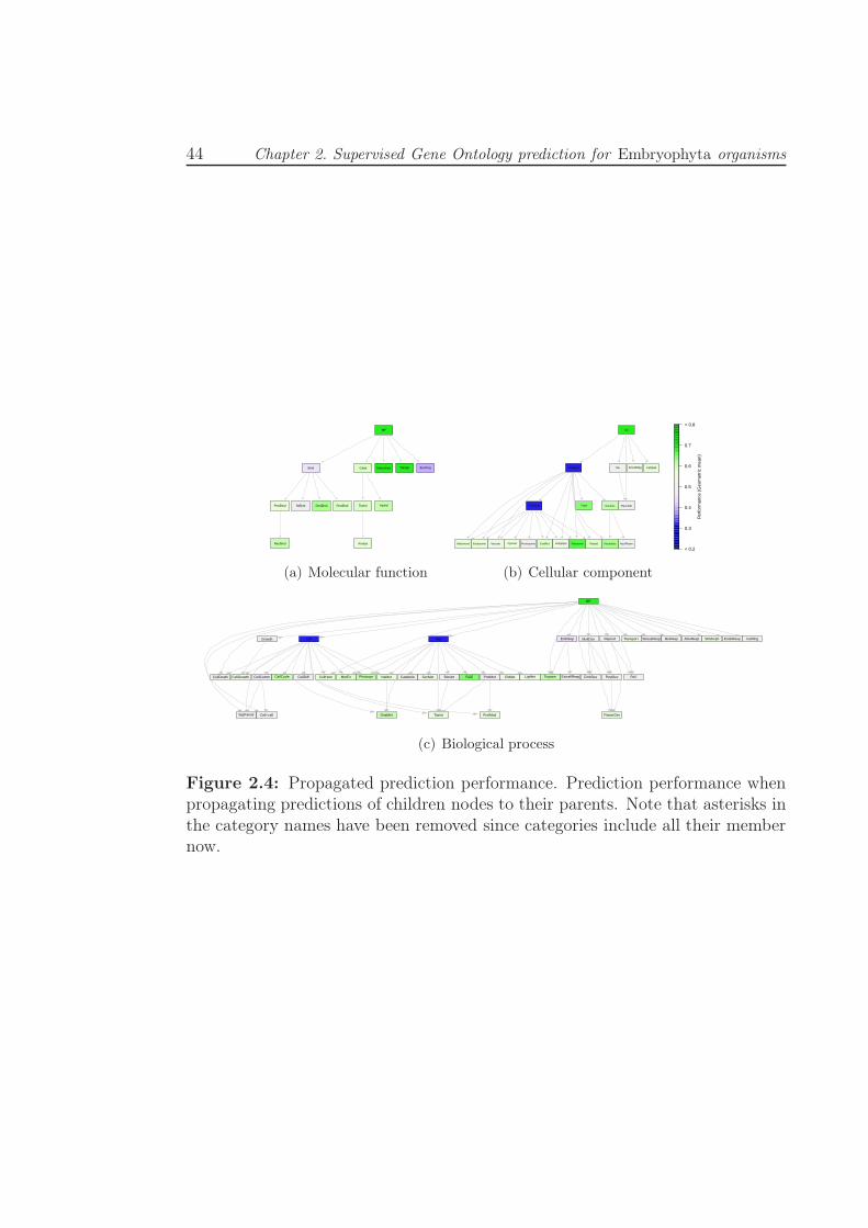
44 Chapter 2. Supervised Gene Ontology prediction for Embryophyta organisms
Bind
MF
ProtBind Transf
Catal
NtBind DnaBind
TranscFact
RnaBind
RecBind
Transp
Kinase
Hydrol
EnzReg
(a) Molecular function
CC
Intracell
NucleusCytPlasm
Mb ExtcellReg CellWall
NuclPlasmNucleolusMitochond Endosome Vacuole Perixosome EndRet GolgiAppCytosol Ribosome
PlasmMb
Plastid
Thylk
< 0.2
0.3
0.4
0.5
0.6
0.7
> 0.8
Per
form
ance
(G
eom
etric
mea
n)
(b) Cellular component
BP
MetCP
NaMet Biosint ProtMetCellComm
ExtResp MultDev Reprod
PostDev
Growth
ChMetMetEn
DnaMet Transl ProtMod
LipMet
Transport StressResp
CellCycle
SigTransd Cell−cell
CellDeath Catabolic Tropism
BioResp AbioResp StrMorph EndoResp
EmbDev Poll
FlowerDev
ExtcellRespPhotosyn
CellOrg
CellGrowth CellHom SecMetCellDiff RGE
(c) Biological process
Figure 2.4: Propagated prediction performance. Prediction performance whenpropagating predictions of children nodes to their parents. Note that asterisks inthe category names have been removed since categories include all their membernow.
2.4. Concluding remarks 45
therefore associated to the nucleus) presented high discriminability from the ex-
tracted features. Ribosomal and other proteins involved with translation, proved
to be highly predictable from features related to electric charges of the amino acid
sequence. At the biological process level, proteins related to regulation of gene
expression and nucleic acid metabolic process were easily predicted, while some
other biological processes showed low predictability from the extracted primary
structure features.

Chapter 3
Semi-supervised Gene Ontology
prediction for Embryophyta
organisms
Supervised machine learning uses a labeled set of instances to train the classifier.
Labeled instances, however, are often difficult, expensive, or time consuming to
obtain, as they require the efforts of experienced human annotators. Meanwhile
unlabeled data may be relatively easy to collect, but there has been few ways to
use them (Zhu, 2007).
In the particular case of protein function prediction, it is a known fact that
only a small number of proteins have actually been annotated for certain func-
tions. Therefore, it is difficult to obtain sufficient training data for the supervised
learning algorithms and, consequently, the tools for protein function prediction
have very limited scopes (Zhao et al., 2008c). Besides, it is particularly hard to
find the representative negative samples because the available information in the
annotation databases, such as Gene Ontology (GO) (The Gene Ontology Con-
sortium, 2004), only provides information about which protein belongs to which
functional class but there is no certainty about which protein does not belong to
the class (Zhao et al., 2008a). To see this, consider the functional path of a GO
term as the path on the ontology from the root to the node representing that GO
term. Since the current functional annotation might be incomplete, it is hard to
48 Chapter 3. Semi-supervised Gene Ontology prediction for Embryophyta organisms
justify whether or not the proteins annotated with the nodes on the functional
paths of a GO node (the ancestors of the term) would belong to this GO node if
a deeper study was performed. Therefore these proteins must only be considered
as unlabeled samples regarding that GO term (Bi et al., 2007).
Under such circumstances, semi-supervised learning methods provide an al-
ternative approach to protein annotation (Zhao et al., 2008c). Semi-supervised
learning (SSL) is halfway between supervised and unsupervised learning: in ad-
dition to labeled data, the algorithm is provided with an amount of unlabeled
data that can be used to improve the estimations about the data. This chap-
ter presents an analysis of the predictability of GO terms with semi-supervised
learning methods, also providing an analysis of the assumptions that the different
methods do, in order to understand their successfulness.
3.1 State of the art in semi-supervised classifica-
tion
The idea of using both labeled and unlabeled data for designing robust predic-
tors has been on the machine learning community since around the middle sixties
with several proposals on self-training, where a supervised learning method is
iteratively re-trained with its own predictions over a set of unlabeled data for
successively refining the final output (see, for example, Scudder III (1965) and
Fralick (1967)). Later, the work in semi-supervised learning moved to the gen-
erative models, considering that each class has a Gaussian distribution. This is
equivalent to assuming that the complete data comes from a mixture model and,
with large amount of unlabeled data, the mixture components can be identified
with the expectation-maximization (EM) algorithm (McLachlan and Krishnan,
2007; Miller and Uyar, 1996). The interest in semi-supervised learning increased
in the nineties, mostly due to applications in natural language problems and text
classification (Blum and Mitchell, 1998; Joachims, 1999). According to Chapelle
and Schölkopf (2006), the work by Merz et al. (1992) was the first to use the
term “semi-supervised” for classification with both labeled and unlabeled data.

3.1. State of the art in semi-supervised classification 49
A more complete historical perspective of semi-supervised learning can be found
on (Chapelle and Schölkopf, 2006, chapter 1).
One significant difference between supervised and semi-supervised methods is
that, unlike supervised learning, in which a good generic learning algorithm can
perform well on a lot of real-world data sets without specific domain knowledge,
in semi-supervised learning there is commonly accepted that there is no “black
box” solution and a good understanding of the nature of the data is required to
achieve successful performance (Chapelle and Schölkopf, 2006, Chapter 21). This
is mainly due to the fact that, in order to deal with labeled and unlabeled data,
current semi-supervised algorithms have to make strong assumptions about the
underlying joint probability measure P (X,Y) e.g. a relation of the probability
of the feature space P (X) and the joint probability of the feature space and the
label set P (Y,X). There are several different semi-supervised learning methods,
and each one makes different assumptions about this link. These methods include
generative models, graph-based models, semi-supervised support vector machines,
and so on (Zhu and Goldberg, 2009).
The main assumption made by semi-supervised learning algorithms is the
“semi-supervised smoothness assumption” (Chapelle and Schölkopf, 2006, chapter
1):
Semi-supervised smoothness assumption: If two points x1, and x2 in a
high-density region are close, then so should be their corresponding label
sets y1, y2. Note that by transitivity, this assumption implies that if two
points are linked by a path of high density (e.g., if they belong to the same
cluster), then their outputs are likely to be close. If, on the other hand,
they are separated by a low-density region, then their outputs need not be
close.
Such assumption originates the two common assumptions used in semi-supervised
learning:
Cluster assumption: If points are in the same cluster, they are likely to be
of the same class. This assumption does not imply that each class forms
a single, compact cluster, it only means that thera are no instances of

50 Chapter 3. Semi-supervised Gene Ontology prediction for Embryophyta organisms
two distinct classes in the same cluster. The cluster assumption can be
formulated in an equivalent way:
Low density separation: The decision boundary should lie in a low-density
region.
Manifold assumption: The (high-dimensional) data lie (roughly) on a low-
dimensional manifold. Instances that are close according to the manifold
geodesic distance are likely to be of the same class.
According to each assumption, there are three main families of semi-supervised
methods: generative methods (cluster assumption), density-based methods (low
density separation), and graph-based methods (manifold assumption). In the
following sub-sections each family of methods will be reviewed, emphasizing on
the assumptions made by each one. It should be pointed out that, since semi-
supervised learning is a rapidly evolving field, the review is necessarily incomplete.
A wider review in this matter can also be found on (Zhu and Goldberg, 2009).
3.1.1 Generative methods
Generative methods follow a common strategy of augmenting the set of labeled
samples with a large set of unlabeled data and combining the two sets with
the Expectation-Maximization algorithm, in order to improve the parameter es-
timates Cozman et al. (2003). They assume a probabilistic model p(x, y) =
p(y)p(x|y), where p(x|y) is an identifiable mixture distribution. The most com-
monly employed distributions are the Gaussian Mixture Models:
p(x|y) =K∑
k=1
πkN(x|θ) (3.1)
where N(x|θ) is the gaussian distribution with parameters θ = [µk,Σk], being µk
the mean vector and Σk the covariance matrix of the k−th Gaussian component,
and πk the mixing components such that∑K
k=1 πk = 1 for k = 1, 2, . . . , K.
Ideally only one labeled example per component is needed to fully determine
the mixture distribution. In this setting, any additional information on p(x)

3.1. State of the art in semi-supervised classification 51
is useful and the EM algorithm can be used for estimating θ. A strength of
the generative approach is that knowledge of the structure of the problem or the
data can naturally be incorporated by modeling it (Chapelle and Schölkopf, 2006,
chapter 1). However, generative techniques provide an estimate of p(x) along the
way, although this is not required for classification, and in general this proves
wasteful given limited data. For example, maximizing the joint likelihood of a
finite sample need not lead to a small classification error, because depending on
the model it may be possible to increase the likelihood more by improving the fit
of p(x) than the fit of p(y|x) (Chapelle and Schölkopf, 2006, chapter 2).
The aforementioned works of Miller and Uyar (1996) and McLachlan and
Krishnan (2007), among others, shown to be strong methods for classifying text
data. Also, Nigam et al. (2000) have applied the EM algorithm on mixture of
multinomial for the task of text classification, showing better performance than
those trained only from the supervised set. Fujino et al. (2005) extend generative
mixture models by including a “bias correction” term and discriminative training
using the maximum entropy principle. However, anecdotal evidence is that many
more studies were not published because they obtained negative results, showing
that learning a mixture model will often degrade the performance of a model fit
using only the labeled data (Zhu and Lafferty, 2005); one published study with
these conclusions is Cozman et al. (2003). This is due to the strong assumption
done by generative methods: that the data actually comes from the mixture
model, where the number of components, prior p(y), and conditional p(x|y) are
all correct (Zhu and Goldberg, 2009).
3.1.2 Density-based methods
With the rising popularity of support vector machines (SVMs), Semi-Supervised
SVMs (S3VMs) emerged as an extension to standard SVMs for semi-supervised
learning. S3VMs find a labeling for all the unlabeled data, and a separating
hyperplane, such that maximum margin is achieved on both the labeled data and
the (now labeled) unlabeled data. As a result, unlabeled data guides the decision
boundary away from dense regions. The assumption of S3VMs is that the classes
are well-separated, such that the decision boundary falls into a low density region

52 Chapter 3. Semi-supervised Gene Ontology prediction for Embryophyta organisms
in the feature space, and does not cut through dense unlabeled data (Zhu and
Goldberg, 2009, chapter 6).
In a similar way than the conventional SVMs described in section 4.1.2, the
optimization problem for an S3VMs can be stated as follows:
θ∗ = argminθ∈T
{1
2||θ||2 + C
L∑
i=1
ℓ (fθ(xi)yi) + λL+U∑
i=L+1
ℓ (|fθ(xi)|)
}(3.2)
where ℓ(t) = max(0, 1− t) is the hinge loss function, C is the trade-off parameter
and λ is a new regularization parameter. The first two terms in the above equation
correspond to the traditional solution for the standard supervised SVM shown in
equation (2.2), while the last term puts fθ(xi) of the unlabeled points xi away
from 0 (thereby implementing the low density assumption) (Chapelle et al., 2006).
Again, as in the supervised case, the kernel trick can be used for constructing
non-linear S3VMs. While the optimization in SVM is convex and can be solved
with QP-hard complexity, optimization in S3VM is a non-convex combinatorial
task with NP-Hard complexity. Most of the recent work in S3VM has been fo-
cused on the optimization procedure (a full survey in this matter can be found in
(Chapelle et al., 2008)). Among the proposed methods for solving the non-convex
optimization problem associated with S3VMs, one of the first implementations is
the S3VMlight by (Joachims, 1999), which is based on local combinatorial search
guided by a label switching procedure. Chapelle and Zien (2005) presented a
method based on gradient descent on the primal, that performs significantly bet-
ter than the optimization strategy pursued in S3VMlight; the work by Chapelle
et al. (2006) proposes the use of a global optimization technique known as “con-
tinuation”, often leading to lower test errors than other optimization algorithms;
Collobert et al. (2006) uses the Concave-Convex procedure, providing a highly
scalable algorithm in the nonlinear case.
Other recent proposals include (Li et al., 2010) which focuses on the class-
imbalance problem and proposes a cost-sensitive S3VM; Qi et al. (2012) which
describes laplacian twin support vector machines; and several approaches to adap-
tive regularizations like (Xu et al., 2009) and (Wang et al., 2011).

3.1. State of the art in semi-supervised classification 53
3.1.3 Graph-based methods
Graph-based methods start with a graph where the nodes are the labeled and
unlabeled data points, and (weighted) edges reflect the similarity of nodes. The
assumption is that nodes connected by a large-weight edge tend to have the same
label, and labels can propagate throughout the graph. In other words, graph-
based methods do the assumption that labels are “smooth” with respect to the
graph, such that they vary slowly on the graph. That is, if two instances are
connected by a strong edge, their labels tend to be the same (Zhu and Goldberg,
2009, chapter 5).
This family of methods enjoy nice properties from spectral graph theory. They
commonly use an energy function as objective in the optimization problem, en-
suring that the labels will change slowly through the graph (consequently im-
plementing the manifold assumption) (Hein et al., 2005). Some common graphs
include the following (Zhu and Goldberg, 2009, chapter 5):
Fully connected graphs: The graph needs to be weighted so that similar nodes
have large edge weight between them. The disadvantage is in computational
cost as the graph is dense. A common choice in this case is the “exp-weighted
graph” where the weights between instances xi and xj are defined as:
Wij = exp(−‖xi − xj‖
2
2α) (3.3)
where α is a bandwidth hyperparameter that controls the decay rate.
Sparse graphs: In this kind of graphs each node connects to only a few nodes,
making them computationally fast. They also tend to enjoy good empirical
performance. There are two common choices: k−NN graphs and ǫ−NN
graphs. In the former, instances xi and xj are connected by an edge if
any of them are included into the k nearest neighbors of the other. k is a
hyperparameter that controls the density of the graph. Small k may result
in disconnected graphs. For ǫ−NN graphs, xi and xj are connected by
an edge, if the distance ‖xi − xj‖ ≤ ǫ. The hyperparameter ǫ controls
neighborhood radius.

54 Chapter 3. Semi-supervised Gene Ontology prediction for Embryophyta organisms
A graph is represented by the (L+U)× (L+U) weight matrix W , Wij = 0 if
there is no edge between instances xi and xj. Once the graph has been defined,
a real function over the nodes can be defined fθ : X → R. In order to achieve
that unlabeled points that are similar (as determined by the edges of the graph)
to have similar labels, the quadratic energy function can be used as objective:
θ∗ = argminθ∈T
{1
2
∑
ij
Wij(fθ(xi)− fθ(xj))2
}(3.4)
Since this objective function is minimized by constant functions, it is necessary
to constrain fθ to take values fθ(xi) = yi, for all the labeled data xi ∈ XL. Finally,
let D be the diagonal degree matrix, where Dii =∑
j Wij is the degree of node
xi. The combinatorial Laplacian ∆ is defined as:
∆ ≡D −W (3.5)
and it is easy to verify that:
θ∗ = argminθ∈T
{fTθ∆fθ
}(3.6)
There are many related methods that exploit the idea of obtaining a target
function being smooth on the graph. Such methods include, among others, the
Mincut (Blum and Chawla), which partitiones the graph for minimizing the num-
ber of pairs of linked instances with different labels; graph random walks (Azran,
2007); harmonic functions (Zhu and Lafferty, 2005); local and global consistency
(Zhou et al., 2004) and manifold regularization (Belkin et al., 2006; Sindhwani
et al., 2006). Some more recent proposals have focused on the problem of large
graph construction, like Liu et al. (2010) and Lin (2012).
Most graph-based methods are inherently transductive, giving predictions for
only those points in the unlabeled set, and not for an arbitrary test point. The
simplest strategy for extending the method for unseen data is by dividing the
input space into Voronoi cells centered on the labeled instances. From an algo-
rithmic point of view, this strategy is equal to classify instances by its 1-nearest-
neighbor. Zhu and Lafferty (2005) proposed an approach that combines genera-
tive mixture models and discriminative regularization using the graph Laplacian
3.1. State of the art in semi-supervised classification 55
in order to provide an inductive model. Laplacian SVMs, proposed by Belkin
et al. (2006), provides a natural inductive algorithm since it uses a modified SVM
for classification. The optimization problem in this case is regularized by the
introduction of a term for controlling the complexity of the model according to
equation (3.6):
θ∗ = argminθ∈T
{∑
i
ℓ (fθ(xi)yi) + λ∑
ij
Wij (fθ(xi)− fθ(xj))2
}(3.7)
where Wij is the weight between the i−th and j−th instances in the graph and λ is
again a regularization parameter. A lot of experiments show that Laplacian SVM
achieves state of the art performance in graph-based semi-supervised classification
Qi et al. (2012).
3.1.4 Applicatons of semi-supervised learning for protein
function prediction
A few semi-supervised methods have been applied for both gene function predic-
tion (over the DNA sequence) and protein function prediction (over the amino
acids sequence). Kasabov and Pang (2003) used a S3VMs for promoter recogni-
tion, improving predictive performance by 55% over the standard inductive SVM
results. Li et al. (2003) used a “co-updating” schema of two SVMs, each one
trained over a different source of data, for discriminating among five functional
classes in the yeast genome. For the problem of predicting the functional proper-
ties of proteins, Krogel and Scheffer (2004) conducted an extensive study on the
caveats of incorporating semi-supervised learning and transduction for predict-
ing various functional properties of proteins corresponding to genes in the yeast
genome, founding that S3VMs significantly decrease performance compared to in-
ductive SVMs. Shin and Tsuda (2006) used graph-based semi-supervised learning
for functional class prediction of yeast proteins, using protein interaction networks
for obtaining the graphs.
More recently, King and Guda (2008) proposes a generative semi-supervised
method for protein functional classification and provide experimental results of

56 Chapter 3. Semi-supervised Gene Ontology prediction for Embryophyta organisms
classifying a set of eukaryotic proteins into seven subcellular locations from the
Cellular Component ontology of GO. Zhao et al. (2008b) proposed a new algo-
rithm to define the negative samples in protein function prediction. In detail,
the one-class SVMs and two-class SVMs are used as the core learning algorithm
in order to identify the representative negative samples so that the positive sam-
ples hidden in the unlabeled data can be recovered. Shin et al. (2009) propose
a method for integrating multiple graphs within a framework of semi-supervised
learning and apply the method to the task of protein functional class predic-
tion in yeast. The proposed method performs significantly better than the same
algorithm trained on any single graph.
3.2 Proposed methodology: semi-supervised learn-
ing for predicting gene ontology terms in Em-
bryophyta plants
3.2.1 Selected semi-supervised algorithms
In order to test the efficiency of semi-supervised learning in the task of predicting
protein functions, two state of the art methods were chosen, each one imple-
menting a different semi-supervised assumption: S3VM following the concave-
convex optimization procedure (CCP) (Collobert et al., 2006) (implementing the
low-density separation assumption and consequently the cluster assumption) and
Laplacian-SVM Belkin et al. (2006) (implementing the manifold assumption).
CCP S3VM: The S3VM proposed by (Collobert et al., 2006; Sinz et al., 2007)
was chosen since it provides high scalability in the nonlinear case, making
it the most suitable choice for the amounts of Embryophyta proteins in the
databases used in this work. Consider the set of labeled points XL = {xi}Li=1
for which labels {yi}Li=1 are provided, and the points XU = {xi}L+Ui=L+1 the
labels of which are not known. The objective function to be optimized in

3.2. Proposed methodology: semi-supervised learning for predicting gene ontology terms
in Embryophyta plants 57
this case, corresponds to:
JS3VM(θ) =1
2||θ||2 + C
L∑
i=1
ℓ (fθ(xi)yi) + λL+U∑
i=L+1
ℓ (|fθ(xi)|) (3.8)
where the function ℓ(t) = max(0, 1 − |t|) is the hinge loss function. The
main problem with this objective function, in contrast to the classical SVM
objective, is that the additional term is non-convex and gives rise to local
minima. Additionally, it has been experimentally observed that the objec-
tive function tends to give unbalanced solutions, classifying all the unlabeled
points in the same class. A constraint should be imposed on the data to
avoid this problem (Chapelle and Zien, 2005):
1
L
L∑
i=1
yi =1
U
L+U∑
i=L+1
fθ(xi) (3.9)
which ensures that the number of unlabeled samples assigned to each class
will be the same fraction as in the labeled data. CCP decomposes a non-
convex function J into a convex component Jvex and a concave component
Jcave. At each iteration, the concave part is replaced by the tangential
approximation at the current point and the sum of this linear function and
the convex part is minimized to get the next iterate. The first two terms
in equation (3.8) are convex, while the third term can be decomposed into
the sum of a convex function plus a concave one:
Jvex = max(0, 1− |t|) + 2|t| (3.10)
Jcave = −2|t| (3.11)
If an unlabeled point is currently classified positive, then at the next itera-
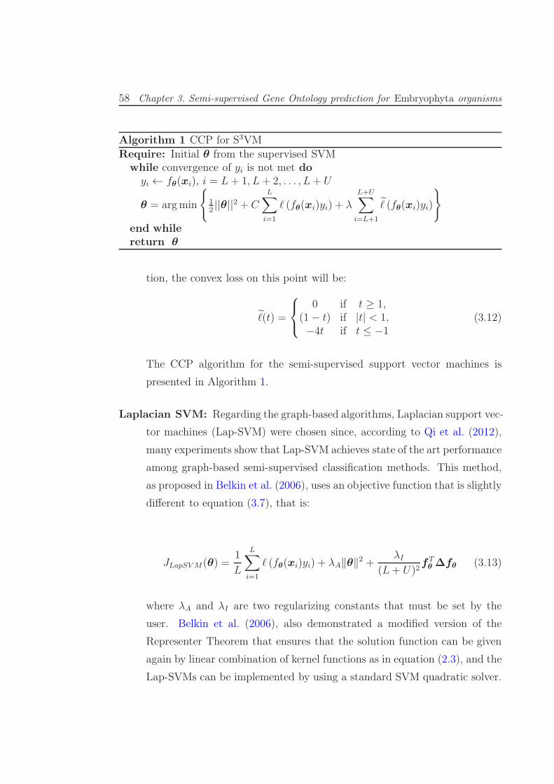
58 Chapter 3. Semi-supervised Gene Ontology prediction for Embryophyta organisms
Algorithm 1 CCP for S3VMRequire: Initial θ from the supervised SVM
while convergence of yi is not met doyi ← fθ(xi), i = L+ 1, L+ 2, . . . , L+ U
θ = argmin
{12||θ||2 + C
L∑
i=1
ℓ (fθ(xi)yi) + λL+U∑
i=L+1
ℓ̃ (fθ(xi)yi)
}
end whilereturn θ
tion, the convex loss on this point will be:
ℓ̃(t) =
0 if t ≥ 1,(1− t) if |t| < 1,−4t if t ≤ −1
(3.12)
The CCP algorithm for the semi-supervised support vector machines is
presented in Algorithm 1.
Laplacian SVM: Regarding the graph-based algorithms, Laplacian support vec-
tor machines (Lap-SVM) were chosen since, according to Qi et al. (2012),
many experiments show that Lap-SVM achieves state of the art performance
among graph-based semi-supervised classification methods. This method,
as proposed in Belkin et al. (2006), uses an objective function that is slightly
different to equation (3.7), that is:
JLapSVM(θ) =1
L
L∑
i=1
ℓ (fθ(xi)yi) + λA‖θ‖2 +
λI
(L+ U)2fTθ∆fθ (3.13)
where λA and λI are two regularizing constants that must be set by the
user. Belkin et al. (2006), also demonstrated a modified version of the
Representer Theorem that ensures that the solution function can be given
again by linear combination of kernel functions as in equation (2.3), and the
Lap-SVMs can be implemented by using a standard SVM quadratic solver.

3.2. Proposed methodology: semi-supervised learning for predicting gene ontology terms
in Embryophyta plants 59
3.2.2 Databases
Before proceeding with the prediction of protein functions, a set of three bench-
mark problems constructed by Chapelle and Schölkopf (2006) was used to test the
algorithms in order to provide an analysis of the relation between the performance
of the semi-supervised learning methods and the different dataset structures. The
benchmark were artificially created in order to create situations that correspond
to certain assumptions. The three datasets have 750 instances, from wich 100 are
labeled while the remaining are unlabeled.
g241n This data set was constructed to have potentially misleading cluster struc-
ture, and no manifold structure. It has 375 points drawn from each of two
unit-variance isotropic Gaussians, the centers of which have a distance of
6 in a random direction; these points form the positive class. Then the
centers of two further Gaussians for the negative class were fixed by moving
from each of the former centers a distance of 2.5 in a random direction. The
identity matrix was used as covariance matrix, and 375 points were sam-
pled from each new Gaussian. A two-dimensional projection of the resulting
data is shown on Figure 3.1(a).
g241c This data set accomplishes the cluster assumption, that is, the classes
correspond to clusters but the manifold assumption does not hold. It has
750 points drawn from each of two unit-variance isotropic Gaussians, the
centers of which had a distance of 2.5 in a random direction. The class
label of a point represents the Gaussian it was drawn from. All dimensions
are standardized (shifted and rescaled to zero-mean and unit variance). A
two-dimensional projection of the resulting data is shown on Figure 3.1(b).
Digit1 This data set was designed to consist of points close to a low-dimensional
manifold embedded into a high-dimensional space, but not to show a pro-
nounced cluster structure. It comes from a system that generates artificial
writings (images) of the digit “1” (Hein and Audibert, 2005). The numbers
are generated from a function with five degrees of freedom and a sequence
of transformations is later applied to introduce noise and different biases

60 Chapter 3. Semi-supervised Gene Ontology prediction for Embryophyta organisms
−6 −4 −2 0 2 4 6
−4
−2
02
4
x1
x 2
(a) g241n
−4 −2 0 2 4
−4
−2
02
4
x1
x 2(b) g241c
Figure 3.1: Two-dimensional projections of the benchmark datasets. Filledcircles represent labeled data while empty circles represent unlabeled data.
to the images. The data will therefore lie close to a five-dimensional man-
ifold. Figure 3.2(b), taken from Chapelle and Schölkopf (2006), shows one
of the original images in the dataset (Figure 3.2(a)) and the transformed
one (Figure 3.2)
For the protein function prediction task, the database described in section
2.2.1 was used as the set of labeled instances. Then, all the available Em-
bryophyta proteins at UniProtKB/Swiss-Prot database that has no entries in
the GOA project were added as the core set of unlabeled instances. As discussed
in the introduction to this chapter, the proteins associated to the nodes in the
functional path of a GO term, were also left as unlabeled instances regarding that
classifier. Finally, 30000 unlabeled instances were randomly chosen in order to
accomplish an approximate relation of ten unlabeled instances per each labeled
one (remember from section 2.2.1 that the set of labeled protein sequences com-
prises 3368 instances). All the unalebeled sequences were characterized according
to the procedure described in section 2.2.3 and the same feature selection strategy
from section 2.2.5.
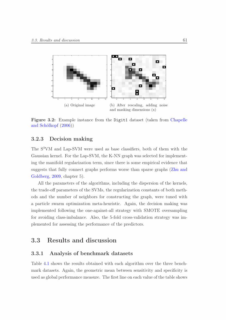
3.3. Results and discussion 61
(a) Original image (b) After rescaling, adding noiseand masking dimensions (x)
Figure 3.2: Example instance from the Digit1 dataset (taken from Chapelleand Schölkopf (2006))
3.2.3 Decision making
The S3VM and Lap-SVM were used as base classifiers, both of them with the
Gaussian kernel. For the Lap-SVM, the K-NN graph was selected for implement-
ing the manifold regularization term, since there is some empirical evidence that
suggests that fully connect graphs performs worse than sparse graphs (Zhu and
Goldberg, 2009, chapter 5).
All the parameters of the algorithms, including the dispersion of the kernels,
the trade-off parameters of the SVMs, the regularization constants of both meth-
ods and the number of neighbors for constructing the graph, were tuned with
a particle swarm optimization meta-heuristic. Again, the decision making was
implemented following the one-against-all strategy with SMOTE oversampling
for avoiding class-imbalance. Also, the 5-fold cross-validation strategy was im-
plemented for assessing the performance of the predictors.
3.3 Results and discussion
3.3.1 Analysis of benchmark datasets
Table 4.1 shows the results obtained with each algorithm over the three bench-
mark datasets. Again, the geometric mean between sensitivity and specificity is
used as global performance measure. The first line on each value of the table shows

62 Chapter 3. Semi-supervised Gene Ontology prediction for Embryophyta organisms
Table 3.1: Performance over the three benchmark sets. Each position shows“mean ± standard deviation” and the corresponding p-value. Highlighted valuesare significantly better than the supervised SVM.
Dataset SVM S3VM Lap-SVM
g241n0.76± 0.11 0.80± 0.12 0.80± 0.07
– 0.43 0.34
g241c0.61± 0.07 0.76± 0.13 0.58± 0.16
– 0.03 0.70
Digit10.85± 0.10 0.87± 0.13 0.92± 0.06
– 0.69 0.09
“mean ± standard deviation” across the five repetitions of the cross-validation
procedure. The second line shows the corresponding p-value for a paired t-test
between the semi-supervised methods and the supervised SVM. Bold face val-
ues indicate which values are significantly better than the supervised SVM for a
paired t-test at 90% significance level.
As expected, S3VM shows a superior performance for the dataset implement-
ing the cluster assumption, while Lap-SVM outperforms the supervised SVM
in the dataset that implements the manifold assumption. None of the semi-
supervised methods is able to outperform the supervised algorithm when none of
the semi-supervised assumptions holds. This is perhaps the most important issue
when dealing with semi-supervised learning: previous knowledge of the nature of
the data is required to select the appropriate learning model.
3.3.2 Analysis of GO prediction in Embryophyta plants
Figure 3.3 shows a comparison between the results with the S3VM (orange line)
and the SVM method presented in chapter 2 (green line). The results with the su-
pervised SVM are the same as in Figure 2.3, but the classes are ordered this time
according to the performance of the SS3VM method. Again, left plots show sensi-
tivity, specificity and geometric mean achieved with the five-fold cross-validation
procedure, while right plots depicts the corresponding p-values obtained from a
paired t-test at a 95% significance level. Orange bars show the cases when the
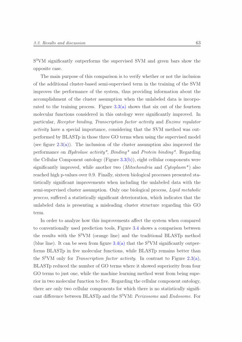
3.3. Results and discussion 63
S3VM significantly outperforms the supervised SVM and green bars show the
opposite case.
The main purpose of this comparison is to verify whether or not the inclusion
of the additional cluster-based semi-supervised term in the training of the SVM
improves the performance of the system, thus providing information about the
accomplishment of the cluster assumption when the unlabeled data is incorpo-
rated to the training process. Figure 3.3(a) shows that six out of the fourteen
molecular functions considered in this ontology were significantly improved. In
particular, Receptor binding, Transcription factor activity and Enzime regulator
activity have a special importance, considering that the SVM method was out-
performed by BLASTp in those three GO terms when using the supervised model
(see figure 2.3(a)). The inclussion of the cluster assumption also improved the
performance on Hydrolase activity*, Binding* and Protein binding*. Regarding
the Cellular Component ontology (Figure 3.3(b)), eight cellular components were
significantly improved, while another two (Mitochondria and Cytoplasm* ) also
reached high p-values over 0.9. Finally, sixteen biological processes presented sta-
tistically significant improvements when including the unlabeled data with the
semi-supervised cluster assumption. Only one biological process, Lipid metabolic
process, suffered a statistically significant deterioration, which indicates that the
unlabeled data is presenting a misleading cluster structure regarding this GO
term.
In order to analyze how this improvements affect the system when compared
to conventionally used prediction tools, Figure 3.4 shows a comparison between
the results with the S3VM (orange line) and the traditional BLASTp method
(blue line). It can be seen from figure 3.4(a) that the S3VM significantly outper-
forms BLASTp in five molecular functions, while BLASTp remains better than
the S3VM only for Transcription factor activity. In contrast to Figure 2.3(a),
BLASTp reduced the number of GO terms where it showed superiority from four
GO terms to just one, while the machine learning method went from being supe-
rior in two molecular function to five. Regarding the cellular component ontology,
there are only two cellular components for which there is no statistically signifi-
cant difference between BLASTp and the S3VM: Perixosome and Endosome. For

64 Chapter 3. Semi-supervised Gene Ontology prediction for Embryophyta organisms
NtBind
EnzReg
Catal*
DnaBind
ProtBind*
Bind*
Kinase
RnaBind
MF*
Transf*
Hydrol*
Transp
TranscFact
RecBind
0.0 0.2 0.4 0.6 0.8 1.0
Sensitivity
Specificity
S3VM
SVM
Performance
0.0 0.2 0.4 0.6 0.8
1 - (p-value)
0.91
0.93
0.73
0.84
0.63
0.89
0.86
0.86
(a) Molecular function
Endosome
PlasmMb
Intracell*
CC*
Mitochond
Perixosome
NuclPlasm
Vacuole
Mb*
CytPlasm*
GolgiApp
CellWall
Cytosol
ExtcellReg
EndRet
Plastid
Nucleus*
Thylk
Nucleolus
Ribosome
0.0 0.2 0.4 0.6 0.8
Sensitivity
Specificity
S3VM
SVM
Performance
0.0 0.2 0.4 0.6 0.8
1 - (p-value)
0.64
0.88
0.87
0.94
0.71
0.93
0.87
0.85
0.89
0.74
0.87
0.86
(b) Cellular component
LipMetTransportBioResp
Met*BP*CP*
CellDeathBiosint*
StressRespExtResp*
CellDiffPoll
EndoRespGrowth*
AbioRespSigTransdStrMorph
ExtcellRespCellComm
NaMet*MultDev*ProtMet*CellOrg
CatabolicChMet
CellGrowthSecMet
PostDev*ProtModEmbDevCellHomReprod*
CellCycleTransl
FlowerDevDnaMetTropism
RGEMetEn
Cell-cellPhotosyn
0.0 0.2 0.4 0.6 0.8
Sensitivity
Specificity
S3VM
SVM
Performance
0.0 0.2 0.4 0.6 0.8
1 - (p-value)
0.68
0.57
0.82
0.92
0.86
0.88
0.92
0.75
0.60
0.80
0.89
0.76
0.90
0.81
0.94
0.88
0.79
0.94
0.75
0.17
0.92
0.88
0.58
0.55
(c) Biological process
Figure 3.3: Comparisson between the S3VM method and the supervised SVM.Bars in the left plots show sensitivity and specificity of the S3VM and lines depictgeometric mean for S3VM (orange) and the classical supervised SVM (green).Right plots depict the p-values obtained by paired t-tests at a 95% significancelevel. For each ontology, the best predicted categories are ordered from top tobottom.
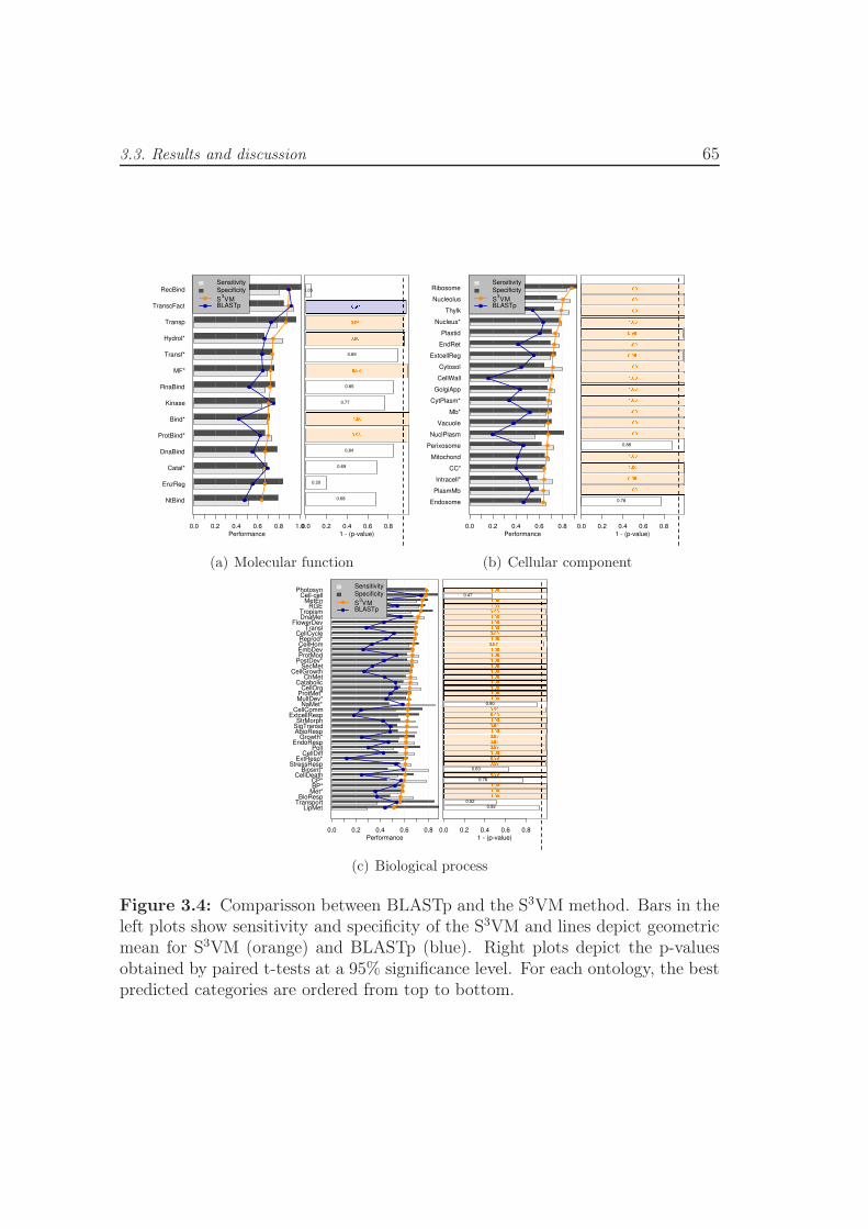
3.3. Results and discussion 65
NtBind
EnzReg
Catal*
DnaBind
ProtBind*
Bind*
Kinase
RnaBind
MF*
Transf*
Hydrol*
Transp
TranscFact
RecBind
0.0 0.2 0.4 0.6 0.8 1.0
Sensitivity
Specificity
S3VM
BLASTp
Performance
0.0 0.2 0.4 0.6 0.8
1 - (p-value)
0.68
0.20
0.69
0.84
0.77
0.85
0.89
0.05
(a) Molecular function
Endosome
PlasmMb
Intracell*
CC*
Mitochond
Perixosome
NuclPlasm
Vacuole
Mb*
CytPlasm*
GolgiApp
CellWall
Cytosol
ExtcellReg
EndRet
Plastid
Nucleus*
Thylk
Nucleolus
Ribosome
0.0 0.2 0.4 0.6 0.8
Sensitivity
Specificity
S3VM
BLASTp
Performance
0.0 0.2 0.4 0.6 0.8
1 - (p-value)
0.78
0.88
(b) Cellular component
LipMetTransportBioResp
Met*BP*CP*
CellDeathBiosint*
StressRespExtResp*
CellDiffPoll
EndoRespGrowth*
AbioRespSigTransdStrMorph
ExtcellRespCellComm
NaMet*MultDev*ProtMet*CellOrg
CatabolicChMet
CellGrowthSecMet
PostDev*ProtModEmbDevCellHomReprod*
CellCycleTransl
FlowerDevDnaMetTropism
RGEMetEn
Cell-cellPhotosyn
0.0 0.2 0.4 0.6 0.8
Sensitivity
Specificity
S3VM
BLASTp
Performance
0.0 0.2 0.4 0.6 0.8
1 - (p-value)
0.92
0.52
0.76
0.63
0.90
0.47
(c) Biological process
Figure 3.4: Comparisson between BLASTp and the S3VM method. Bars in theleft plots show sensitivity and specificity of the S3VM and lines depict geometricmean for S3VM (orange) and BLASTp (blue). Right plots depict the p-valuesobtained by paired t-tests at a 95% significance level. For each ontology, the bestpredicted categories are ordered from top to bottom.

66 Chapter 3. Semi-supervised Gene Ontology prediction for Embryophyta organisms
all the remaining eighteen cellular components, the semi-supervised method ob-
tained superior performance. A similar behavior is shown at figure 3.4(c), where
the S3VM significantly outperforms BLASTp in 35 out of the 41 biological pro-
cesses, while the remaining six process showed no statistical difference between
the methods.
On the other hand, Figure 3.5 shows the comparison between the supervised
SVM and the Laplacian-SVM. This analysis provides information about the im-
pact of incorporating unlabeled data on the training set but, this time, by im-
plementing the semi-supervised manifold assumption. This time, it is possible
to see that there are less GO terms that have been improved by the inclusion
of the unlabeled data. For the molecular function ontology (Figure 3.5(a)), only
the Nucleotide binding and Enzyme regulator activity GO terms were signifi-
cantly improved respecting the supervised SVM; in turn the implementation of
the manifold assumption significantly degraded the performance for the GO term
Transcription factor activity. Regarding the cellular component ontology (Figure
3.5(b)), improvements are present for Perixosome, Vacuole and the root node of
the ontology, while a decrease is evinced for the Nucleus* GO term. As for the bi-
ological process ontology, seven GO terms enhaced their prediction performance (
Embryonic development, Response to extracellular stimulus, Response to external
stimulus*, Metabolic process*, Response to biotic stimulus, Cell communication
and the root node of the ontology), while another two were worsened (Cell cycle
and DNA metabolic process).
Figure 3.6 depicts a comparison between the results obtained with BLASTp
and the Lap-SVM method. The first important result that can be inferred from
the present analyses is that, in general terms, for the problem of protein function
prediction, the semi-supervised cluster assumption holds for many more cases
than the semi-supervised manifold assumption. However, the most important
aspect to be analyzed here, is how the results in Figure 3.6 complement the
results from Figure 3.4. Only two molecular functions presented an statistically
significant superior performance with the Lap-SVM over BLASTp. One of them,
RNA binding, did not show statistical significance when comparing BLASTp and
S3VM. The same behavior is present for the Perixosome cellular component and
for the biological processes Transport and Lipid metabolic process. This results

3.3. Results and discussion 67
EnzReg
Bind*
ProtBind*
MF*
RecBind
Catal*
DnaBind
Hydrol*
Transf*
NtBind
RnaBind
Kinase
TranscFact
Transp
0.0 0.2 0.4 0.6 0.8 1.0
Sensitivity
Specificity
Lap-SVM
SVM
Performance
0.0 0.2 0.4 0.6 0.8
1 - (p-value)
0.43
0.57
0.65
0.89
0.50
0.91
0.21
0.78
0.71
0.83
0.08
(a) Molecular function
Endosome
Intracell*
Mb*
Nucleus*
GolgiApp
CC*
Mitochond
PlasmMb
Cytosol
Plastid
CytPlasm*
Vacuole
EndRet
NuclPlasm
ExtcellReg
CellWall
Perixosome
Nucleolus
Thylk
Ribosome
0.0 0.2 0.4 0.6 0.8
Sensitivity
Specificity
Lap-SVM
SVM
Performance
0.0 0.2 0.4 0.6 0.8
1 - (p-value)
0.51
0.47
0.73
0.66
0.19
0.83
0.34
0.38
0.42
0.41
0.78
0.90
0.91
0.76
0.43
0.35
(b) Cellular component
CellDiffStressResp
AbioRespCellDeath
EndoRespSecMet
PollDnaMet
CellCommGrowth*
BP*LipMet
SigTransdCP*
CellOrgTransportProtMet*ProtMod
CellCycleBioResp
ChMetMultDev*
CellGrowthCatabolic
Cell-cellBiosint*
StrMorphNaMet*
Met*PostDev*ExtResp*
ExtcellRespMetEn
FlowerDevReprod*
TranslEmbDevCellHom
PhotosynTropism
RGE
0.0 0.2 0.4 0.6 0.8
Sensitivity
Specificity
Lap-SVM
SVM
Performance
0.0 0.2 0.4 0.6 0.8 1.0
1 - (p-value)
0.48
0.85
0.67
0.44
0.25
0.10
0.38
0.73
0.77
0.72
0.91
0.83
0.66
0.66
0.51
0.77
0.82
0.90
0.72
0.82
0.90
0.83
0.77
0.94
0.15
0.83
0.59
0.42
0.69
0.05
0.67
0.85
(c) Biological process
Figure 3.5: Comparison between the Lap-SVM method and the supervisedSVM. Bars in the left plots show sensitivity and specificity of the Lap-SVM andlines depict geometric mean for Lap-SVM (orange) and the classical supervisedSVM (green). Right plots depict the p-values obtained by paired t-tests at a 95%significance level. For each ontology, the best predicted categories are orderedfrom top to bottom.

68 Chapter 3. Semi-supervised Gene Ontology prediction for Embryophyta organisms
EnzReg
Bind*
ProtBind*
MF*
RecBind
Catal*
DnaBind
Hydrol*
Transf*
NtBind
RnaBind
Kinase
TranscFact
Transp
0.0 0.2 0.4 0.6 0.8 1.0
Sensitivity
Specificity
Lap-SVM
BLASTp
Performance
0.0 0.2 0.4 0.6 0.8
1 - (p-value)
0.60
0.81
0.90
0.92
0.20
0.17
0.82
0.78
0.01
(a) Molecular function
Endosome
Intracell*
Mb*
Nucleus*
GolgiApp
CC*
Mitochond
PlasmMb
Cytosol
Plastid
CytPlasm*
Vacuole
EndRet
NuclPlasm
ExtcellReg
CellWall
Perixosome
Nucleolus
Thylk
Ribosome
0.0 0.2 0.4 0.6 0.8
Sensitivity
Specificity
Lap-SVM
BLASTp
Performance
0.0 0.2 0.4 0.6 0.8
1 - (p-value)
0.25
0.85
0.27
0.94
0.93
(b) Cellular component
CellDiffStressResp
AbioRespCellDeath
EndoRespSecMet
PollDnaMet
CellCommGrowth*
BP*LipMet
SigTransdCP*
CellOrgTransportProtMet*ProtMod
CellCycleBioResp
ChMetMultDev*
CellGrowthCatabolic
Cell-cellBiosint*
StrMorphNaMet*
Met*PostDev*ExtResp*
ExtcellRespMetEn
FlowerDevReprod*
TranslEmbDevCellHom
PhotosynTropism
RGE
0.0 0.2 0.4 0.6 0.8
Sensitivity
Specificity
Lap-SVM
BLASTp
Performance
0.0 0.2 0.4 0.6 0.8
1 - (p-value)
0.40
0.94
0.93
0.04
0.37
0.92
0.92
0.68
0.59
(c) Biological process
Figure 3.6: Comparison between BLASTp and the Lap-SVM method. Bars inthe left plots show sensitivity and specificity of the Lap-SVM and lines depictgeometric mean for Lap-SVM (orange) and BLASTp (blue). Right plots depictthe p-values obtained by paired t-tests at a 95% significance level. For eachontology, the best predicted categories are ordered from top to bottom.

3.4. Concluding remarks 69
indicate that the manifold assumption is best suited than the cluster assumption
for this particular GO terms. A few GO terms were not improved by any of the
assumptions.
3.4 Concluding remarks
In this chapter, an analysis of the suitability of semi-supervised methods for the
prediction of protein functions in Embryophyta plants was performed. A review
of the state of the art of semi-supervised classifiers was presented, highlighting
the different assumptions that each method does about the underlying distribu-
tion of the data. Two semi-supervised methods were chosen to perform the tests,
each representing one of the main semi-supervised assumptions: cluster assump-
tion and manifold assumption. The results show that semi-supervised learning
applied to the prediction of GO terms in Embryophyta organisms, significantly
outperforms the supervised learning approach, at the same time outperform-
ing the commonly used sequence alignment strategy in most cases. In general
terms, the highest performance were reached when applying the cluster assump-
tion. However, several GO terms that were not significantly improved with the
cluster assumption, achieved higher performance with the manifold based semi-
supervised method, demonstrating that a single assumption is not enough for
improving the learning process by the exploitation of the additional unlabeled
data.


Chapter 4
Semi-supervised learning with
multi-objective optimization
Semi-supervised learning uses unlabeled data to improve the estimation of the
predictor function fθ. However, there are two main concerns in order to correctly
explode the information contained in the unlabeled data. First, as mentioned in
the preceding chapter, each model has to make some specific assumption about
the underlying structure of the data. Then, it turns evident that blindly selecting
a semi-supervised learning method for a specific task will not necessarily improve
performance over supervised learning. In fact, unlabeled data can lead to worse
performance with the wrong assumption (Zhu and Goldberg, 2009, chapter 2).
Second, when integrating unsupervised and supervised information by means of
an objective function, it is not usually clear what the best weighting between
these components will be, and it is possible that the weighting chosen may have
a significant effect on the final outcome (Handl and Knowles, 2006).
In this scenario, managing semi-supervised learning within the framework of
multi-objective optimization, may provide a more flexible tool for the integration
of both unsupervised and supervised components. Specifically, the use of Pareto
optimization provides the means to avoid the need for hard constraints and for
a fixed weighting between unsupervised and supervised objectives (Handl, 2006).
Additionally, since multi-objective optimization allows the integration of multi-
ple individual objectives, it would be possible to integrate several semi-supervised

72 Chapter 4. Semi-supervised learning with multi-objective optimization
assumptions within the same learning process, thus allowing for a wider applica-
bility of the method.
In this chapter, a new method for semi-supervised learning within the frame-
work of multi-objective optimization is proposed. This method combines su-
pervised learning with the semi-supervised cluster and manifold assumptions,
obtaining a flexible strategy that with low dependency on the data distribution.
The efficiency of the method is tested over several toy problems and is finally
employed on the prediction of GO terms for protein function prediction in Em-
bryophyta plants.
4.1 Proposed method
Most density-based methods and graph-based methods reviewed in sections 3.1.2
and 3.1.3, respectively follow a common principle in order to incorporate the
unlabeled samples into a supervised learner: they include an additional regularizer
term into the optimization problem. As shown in equation (3.8), S3VM defines a
regularization term which penalizes functions which vary in high-density regions:
JS3VM(θ) =1
2||θ||2 + C
L∑
i=1
ℓ (fθ(xi)yi) + λ
L+U∑
i=L+1
ℓ (|fθ(xi)|)
where λ is a regularization coefficient that must be set by the user. In the
same way, the optimization criterion defined on equation (3.13) by the Lap-SVM
method, uses a regularizer which prefers functions which vary smoothly along the
manifold:
JLapSVM(θ) =1
L
L∑
i=1
ℓ (fθ(xi)yi) + λA‖θ‖2 +
λI
(L+ U)2fTθ∆fθ
where λA and λI are again two regularization constants that must be fixed by the
user. It is quite straightforward to notice that regularization can be viewed as
a special case of a multi-objective optimization problem, where several objective
functions are being linearly combined by the introduction of linear weights (reg-
ularization constants). The aforementioned equations can be viewed as a special

4.1. Proposed method 73
case of a multi-objective optimization problem where there are a number of pos-
sibly conflicting objective functions {Ji(θ)}Mi=1, and they are linearly combined in
a unique objective function by the introduction of linear weights:
J(θ) = λ1J1(θ) + . . .+ λMJM(θ) (4.1)
Solving the regularized optimization problem for a unique combination of
weights λi, yields to a solution that focuses on the objective functions with the
highest weights. Many authors have demonstrated the inability of the method
to capture Pareto optimal points that lie on non-convex portions of the Pareto
optimal curve (Chen, 1998; Huang et al., 2007). Besides, it is well known that the
method does not provide an even distribution of points in the Pareto optimal set,
but only a linear approximation of the preference function (Marler and Arora,
2009).
A more flexible solution can be obtained by managing the optimization prob-
lem as a multi-objective optimization task, where the objective function produces
a vectorial output of length M :
J(θ) = {J1(θ), . . . , JM(θ)} (4.2)
In this setting, the optimization algorithm does not searches for a unique so-
lution, but for the set of all Pareto-optimal solutions with non-convex trade-off
surfaces. Tackling the semi-supervised classification problem within the frame-
work of multi-objective optimization provide a more flexible framework for the
integration of both unsupervised and supervised components. Specifically, the use
of Pareto optimization provides the means to avoid the need for hard constraints
and for a fixed weighting between unsupervised and supervised objectives. Con-
sequently, one would expect a multi-objective approach to semi-supervised clas-
sification to perform more consistently across different data sets, and to be less
affected by model assumptions.
74 Chapter 4. Semi-supervised learning with multi-objective optimization
4.1.1 Objective functions
Once again, consider a set of labeled instances XL = {xi}Li=1 for which labels
{yi}Li=1 are provided, and a set of unlabeled instances XU = {xi}
L+Ui=L+1 the labels
of which are not known. In principle, a linear decision function will be considered:
fθ(x) = 〈θ,x〉 (4.3)
Three objective functions are proposed in a multi-objective minimization
framework. One for reflecting the error achieved in the classification of the la-
beled training data, and the other two for exploiting the information contained on
the unlabeled samples. A separate objective is defined for each semi-supervised
assumption: low density assumption (and implicitly the cluster assumption) and
the manifold assumption, covering the complete landscape of semi-supervised
assumptions. The proposed objectives are:
Jsup(θ) =1
2||θ||2 + C
L∑
i=1
ℓ (fθ(xi)yi) (4.4)
Jclus(θ) =L+U∑
i=L+1
ℓ (|fθ(xi)|) (4.5)
Jman(θ) =∑
ij
Wij(fθ(xi)− fθ(xj))2 (4.6)
where ℓ(t) = max(0, 1−t) is the hinge loss function, C is a trade-off parameter for
regulating the complexity of the model and Wij is the graph weight connecting
the i−th and j−th instances. The first objective function, Jsup, is the standard
SVM objective function that is minimized when the decision boundary maximizes
the margin between the classes in the labeled instances. The second objective,
Jclus, is minimized when the evaluations fθ(xi) of the unlabeled points xi are
away from 0, that is, when the decision boundary is away from the unlabeled
instances. This ensures the accomplishment of the low density assumption and,
consequently, the cluster assumption. Finally, the third objective function, Jman,
is an energy function that is minimized when the labels change slowly through
4.1. Proposed method 75
the graph, which accomplishes the manifold assumption.
Since these three objectives are not necessarily minimized for the same vector
of parameters θ simultaneously, it is necessary to provide a Pareto optimal set of
solutions {θ∗i}Pi=1 reflecting the trade-offs among the objectives. Then, a single
solution can be selected according to its coherence with the application at hand.
4.1.2 Non-linear mapping
Traditional supervised SVMs can be extended to the non-linear case by using the
kernel trick described in section . This procedure implies mapping the data into a
high dimensional Hilbert space H through a mapping Φ : X 7→ H, where a linear
decision boundary is able to correctly assign the class labels. The mapping Φ can
be explicitly computed or only implicitly through the use of a kernel function K
such that K(x1,x2) = 〈Φ(x1),Φ(x2)〉. A square kernel matrix K can thus be
computed, which elements are given by Kij = K(xi,xj).
However, since the inclusion of the additional objectives does not allow to
express the whole optimization problem in terms of dot products, the optimization
must be performed directly on the feature space. For this purpose is necessary
to consider that, even in the case of a high dimensional feature space H, a finite
training set of size N (for the semi-supervised setting N = L+U), when mapped
to this feature space, spans a vectorial subspace E ⊂ H whose dimension is at
most N (Belkin et al., 2006).
Let {vi}Ni=1 be an orthonormal basis of E, where the p−th vector vp can be
expressed as:
vp =
N∑
i=1
AipΦ(xi) (4.7)
where A is a matrix that necessarily has to satisfy ATKA = I. A possible
solution (among several choices) can be obtained by the eigendecomposition of
K as K = UTΛU , which provides A = UΛ
−1/2. Then, a mapping Ψ : X 7→ RN

76 Chapter 4. Semi-supervised learning with multi-objective optimization
can be computed as:
Ψp(x) =
L∑
i=1
AipK(x,xi), p = 1, 2, . . . , N (4.8)
This mapping satisfies the relation 〈Ψ(xi),Ψ(xj)〉 = K(xi,xj) and can be
used for obtaining a feature space where the linear function fθ provides a non-
linear decision boundary in the original space X.
4.2 Proposed method: multi-objective semi-supervised
learning for predicting GO terms in Embryophyta
plants
4.2.1 Selected multi-objective strategy: cuckoo search
Due to their population-based nature, meta-heuristic algorithms are able to ap-
proximate the whole Pareto front of a multi-objective optimization problem in
a single run. Nowadays, real world applications of large scale multi-objective
optimization are feasible thanks to the developments of this kind of algorithms,
and several review papers and books have been recently published in this matter
(Talbi, 2009; Yang, 2010; Zhou et al., 2011).
Recently, a new meta-heuristic search algorithm called Cuckoo Search (CS)
has been developed by Yang and Deb (2009), and its multi-objective extension,
Multi-Objective Cuckoo Search (MOCS) was lately proposed (Yang and Deb,
2011). MOCS has been tested against a subset of well-chosen test functions, and
have been applied to solve design optimization benchmarks in structural engi-
neering showing a clear superiority in comparison with other algorithms (Yang
and Deb, 2013). This superiority can be attributed to the fact that cuckoo search
uses a combination of vectorized mutation, crossover by permutation and Lévy
flights and selective elitism among the best solutions. In addition, the not-so-good
solutions can be replaced systematically by new solutions, and new solutions are
often generated by preferring quality solutions in the solution sets. Thus, the
mechanism of the overall search moves is more subtle and balanced, compared

4.2. Proposed method: multi-objective semi-supervised learning for predicting GO
terms in Embryophyta plants 77
with the simple mechanism used by other meta-heuristics such as particle swarm
optimization or genetic algorithms.
Cuckoo Search is based on the parasitic behavior exposed by some species of
Cuckoo birds. Its natural strategy consists on leaving eggs in host nests created
by other birds. This eggs presents the particularity to have a big similitude with
host eggs, the more similar they are, the greater is its chance of survival. Based
on this statement, Cuckoo Search uses three idealized rules (Yang and Deb, 2009):
1. Each cuckoo lays one egg at a time, and dumps it in a randomly chosen
nest.
2. The best nests with high quality of eggs (solutions) will carry over to the
next generations.
3. The number of available host nests is fixed, and a host can discover an alien
egg with a probability pa ∈ [0, 1]. In this case, the host bird can either
throw the egg away or abandon the nest so as to build a completely new
nest in a new location.
The fisrt assumption can be achieved by the generation of new random so-
lutions from the existing ones. Such procedure is driven by Lévy flights of the
form:
θ(t+1)i = θ
(t)i + α⊕ Lévy(γ) (4.9)
where α is the step size and the random step is drawn from a Lévy distribution:
Lévy ∼ u = t−γ , (1 < γ ≤ 3) (4.10)
which has an infinite variance with an infinite mean. The steps form a random
walk with a power-law step-length distribution with a heavy tail. Figure 4.1
shows an example of three Lévy flights generated from the same starting point
at (0, 0).
On the other hand, the last assumption can be approximated by replacing
a fraction pa of the Q nests by new nests (with new random solutions at new
locations). Parameters pa and α are directly concerned with the efficiency of

78 Chapter 4. Semi-supervised learning with multi-objective optimization
−2 −1 0 1 2
−2
−1
01
2
θ1
θ 2
Figure 4.1: Example of three Lévy flights of length 100 starting from the origin
the search, allowing to find globally and locally improved solutions, respectively.
Additionally, these parameters directly influence the convergence rate of the op-
timization algorithm. For instance, if the value of pa tends to be small and α
value is large, the algorithm will increment the number of iterations to converge
to an optimal value. On the other hand, if the value of pa is large and α is
small, the convergence speed of the algorithm tends to be very high but it is
more likely to converge to a local optimum. Valian et al. (2011) proposed an
improvement which consists on using a range of pa and α to change dynamically
in each iteration,following the equations:
pa(t) = pmax −t
T(pmax − pmin) (4.11)
α(t) = αmaxe(cT ) (4.12)

4.2. Proposed method: multi-objective semi-supervised learning for predicting GO
terms in Embryophyta plants 79
Algorithm 2 Multi-objective Cuckoo SearchRequire: Objective function J(θ) = [J1(θ), J2(θ), . . . , JM(θ)]Require: Initial population of P host nests {θi}
Pi=1, each one with M eggs
Require: Maximal number of iterations TInitialize the iterations counter t = 0Initialize an empty set of Pareto-optimal solutions P(0) = ∅while (|P| < P ) ∨ (t < T ) do
Get a cuckoo randomly (say i) by Lévy flightsEvaluate and check if the solution is Pareto optimalChoose a nest among P (say j) randomlyEvaluate M solutions for nest jif New solutions of nest j dominate those of nest i then
Replace nest i by the new solution of nest jend ifAbandon a fraction pa of worst nestsSort and find the current Pareto optimal solutions {θ∗}(t) and update theset of global Pareto optimal solutions P(t+1) = P(t) ∪ {θ∗}(t)
end whilereturn P
where t is current iteration, T is the maximum number of iterations, and c is a
constant given by:
c =1
Tlog
(αmin
αmax
)(4.13)
The MOCS algorithm is summarized in Algorithm 2. Notice that the only
free parameters that must be directly chosen by the user are the size of the
population and the maximal number of iterations. While the latter is not of
significant importance as it only provides an “emergency stop” in the cases when
the algorithm does not converge, the former is directly linked to the number
of points in the Pareto front that will be obtained. In order to obtain a good
resolution and maximizing the precision on the estimation of the Pareto front, this
number must be as high as possible. However, it will increase the computational
time for the training. This parameter was empirically fixed to P = 1000 for all
the analysis in this chapter.

80 Chapter 4. Semi-supervised learning with multi-objective optimization
4.2.2 Decision making
As in the previous analyses, the Gaussian kernel and the K-NN graph were se-
lected as base tools for implementing the objective functions. There are only three
free parameters to be tuned this time: the dispersion of the kernel, the trade-off
parameter of the SVM in the supervised objective and the number of nearest
neighbors for constructing the graph in the manifold-based objective. Such pa-
rameters were, once again, tuned the particle swarm optimization strategy. It
is important to remark that, unlike the analyses in the previous chapter, all the
regularization parameters are unnecessary here.
Again, the decision making was implemented following the one-against-all
strategy with SMOTE oversampling for avoiding class-imbalance and 5-fold cross-
validation was implemented for assessing the performance of the predictors. How-
ever, there is one additional step that is necessary for the multi-objective strategy:
selecting the most appropriate solution among the set of Pareto-optimal trade-
offs. This task is usually left to be carried out by a human expert, depending
on his knowledge of the application at hand. In the case of protein functional
prediction, the chosen solution must reflect the biological knowledge about the
problem, which is contained in the set of GO terms associated to each sequence.
To this end, an additional cross-validation step is performed, in order to select
the solution with the highest prediction accuracy, which in turn constitutes the
most biologically feasible solution. Figure 4.2 depicts the complete methodology
for estimating the performance of the proposed method. Every 80/20 split rep-
resents a cross-validation procedure (80/20 is the partitioning for a single fold in
a 5-fold cross-validation schema).
4.3 Results and discussion
In this section, the same datasets described in the preceding chapter (section
3.2.2) are used for obtaining an estimation of the performance of the proposed
method. In order to provide a more detailed analysis on the interpretation of
the Pareto-optimal sets that are obtained from the multi-objective strategy, sev-
eral solution points from the same Pareto front are analyzed in the case of the
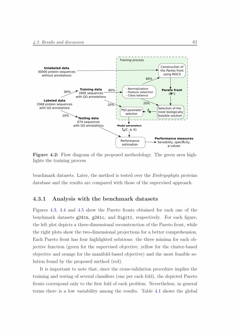
4.3. Results and discussion 81
Labeled data
3368 protein sequences
with GO annotations
Training process
- Normalization
- Feature selection
- Class balance
Training data
2695 sequences
with GO annotations
Testing data
674 sequences
with GO annotations
Construction of
the Pareto front
using MOCS
Selection of the
most biologically
feasible solution
PSO parameter
selection
Performance
estimation
Unlabeled data
30000 protein sequences
without annotations
f
80%
80%
Pareto front
{ *}
80%
20%20%
Model parameters
f�(C, , K)
20%
Performance measures
Sensibility, speci city,
p-values
Figure 4.2: Flow diagram of the proposed methodology. The green area high-lights the training process
benchmark datasets. Later, the method is tested over the Embryophyta proteins
database and the results are compared with those of the supervised approach.
4.3.1 Analysis with the benchmark datasets
Figures 4.3, 4.4 and 4.5 show the Pareto fronts obtained for each one of the
benchmark datasets g241n, g241c, and Digit1, respectively. For each figure,
the left plot depicts a three-dimensional reconstruction of the Pareto front, while
the right plots show the two-dimensional projections for a better comprehension.
Each Pareto front has four highlighted solutions: the three minima for each ob-
jective function (green for the supervised objective, yellow for the cluster-based
objective and orange for the manifold-based objective) and the most feasible so-
lution found by the proposed method (red).
It is important to note that, since the cross-validation procedure implies the
training and testing of several classifiers (one per each fold), the depicted Pareto
fronts correspond only to the first fold of each problem. Nevertheless, in general
terms there is a low variability among the results. Table 4.1 shows the global
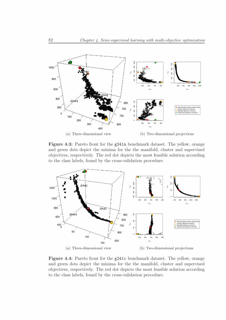
82 Chapter 4. Semi-supervised learning with multi-objective optimization
(a) Three-dimensional view
650 700 750 800
200
400
600
800
1000
Jman
J clu
s
650 700 750 800
010
020
030
040
0
Jman
J sup
200 400 600 800 1000
010
020
030
040
0
Jclus
J sup
Most feasible solution determinedCluster objective minimumManifold objective minimumSupervised objective minimum
(b) Two-dimensional projections
Figure 4.3: Pareto front for the g241n benchmark dataset. The yellow, orangeand green dots depict the minima for the the manifold, cluster and supervisedobjectives, respectively. The red dot depicts the most feasible solution accordingto the class labels, found by the cross-validation procedure.
(a) Three-dimensional view
500 600 700 800 900
400
600
800
1000
Jman
J clu
s
500 600 700 800 900
050
100
150
Jman
J sup
400 600 800 1000 1200
050
100
150
Jclus
J sup
Most feasible solution determinedCluster objective minimumManifold objective minimumSupervised objective minimum
(b) Two-dimensional projections
Figure 4.4: Pareto front for the g241c benchmark dataset. The yellow, orangeand green dots depict the minima for the the manifold, cluster and supervisedobjectives, respectively. The red dot depicts the most feasible solution accordingto the class labels, found by the cross-validation procedure.

4.3. Results and discussion 83
(a) Three-dimensional view
250 300 350 400
200
400
600
800
Jman
J clu
s
250 300 350 400
050
100
150
200
250
Jman
J sup
200 400 600 800 1000
050
100
150
200
250
Jclus
J sup
Most feasible solution determinedCluster objective minimumManifold objective minimumSupervised objective minimum
(b) Two-dimensional projections
Figure 4.5: Pareto front for the Digit1 benchmark dataset. The yellow, orangeand green dots depict the minima for the the manifold, cluster and supervisedobjectives, respectively. The red dot depicts the most feasible solution accordingto the class labels, found by the cross-validation procedure.
performance results for the three benchmark problems, with each one of the
highlighted solutions. Each position in the table shows the mean and standard
deviation across the ten folds of the cross-validation procedure.
There are several interesting results to observe from Table 4.1. First of all,
it must be noted that the proposed method is able to automatically select the
best solution on the Pareto front, implicitly assigning a different weight to each
objective, that is consistent with the nature of the problem. Remember from
section 3.2.2 that the g241n dataset has a misleading structure where unlabeled
data are neither organized on well defined clusters nor on an underlying manifold
structure. In this case, it is possible to observe (see Figure 4.3) that the best
solution found (the red one) is closer to the minimum of the supervised objective
(green dot) than to any other minima. That means that the method assigned a
higher importance to the supervised objective than to the other two. Regarding
the g241c dataset, which has a well defined cluster structure, the best solution
found is consistently closer to the yellow dot (see Figure 4.4) that represents
the minimum of the cluster-based objective. The proper observed on Figure 4.5,

84 Chapter 4. Semi-supervised learning with multi-objective optimization
Table 4.1: Performance over the three benchmark sets for several solutions fromthe Pareto fronts. Each position shows “mean ± standard deviation”. Highlightedvalues on the right are the highest among the three individual objectives.
Dataset Proposed solution Supervised Cluster Manifold
g241n 0.63± 0.008 0.60± 0.031 0.45± 0.068 0.56± 0.014
g241c 0.725± 0.002 0.56± 0.256 0.67± 0.033 0.15± 0.198
Digit1 0.93± 0.005 0.71± 0.264 0.70± 0.159 0.92± 0.011
where the best solution found is very close to the minimum of the manifold-based
objective (orange dot). This is consistent with the nature of the Digit1 dataset
which was designed to have an underlying manifold structure.
The second aspect that must be noted here is that minimizing one single
objective is not enough to achieve the best performance results on any problem.
On all cases,the best results were achieved for a solution on the Pareto front, that
does not exactly matches any of the single-objective minima. Even in the case
of the Digit1 dataset (Figure 4.5), where the best found solution (red) is very
close to the minimum of the manifold-based objective (orange), there is a slight
difference between those solutions that is reflected in the performance on Table
4.1.
Finally, it is worth to note the low standard deviation values achieved by the
proposed method, which demonstrates the reliability of the method in spite of
the random component of the underlying optimization strategy employed.
4.3.2 Analysis of GO prediction in Embryophyta plants
Figure 4.6 shows a comparison between the results with the proposed method
(orange line) and the classical supervised SVM method presented in chapter 2
(green line). Again, left plots show sensitivity, specificity and geometric mean
achieved with the five-fold cross-validation procedure, while right plots depicts
the corresponding p-values obtained from a paired t-test at a 95% significance
level. Orange bars show the cases when the proposed multi-objective method
significantly outperforms the supervised SVM and green bars show the oppo-
site case. This time, Figure 4.6(a) shows that nine molecular functions reached
4.4. Concluding remarks 85
significantly better prediction performance with the proposed method over the
supervised SVM. Also, on the five remaining molecular functions, both methods
achieved statistically similar results, presumably since the unlabeled data is not
contributing to improve the predictions, but in no case the inclusion of this data
degraded the performance of the predictor as it happened with the Lap-SVM in
the preceding chapter (Figure 3.5). A similar behavior was also obtained for the
Cellular Component ontology in Figure 4.6(b), were fifteen out of the 21 con-
sidered cellular components were statistically better predicted by the proposed
method. The same happened also for the Biological Process ontology (Figure
4.6(c)) where only nine out of the whole set of 41 biological processes did not
show an statistically significant improvement.
Finally, Figure 4.7 shows a comparison between the proposed method and
BLASTp. From the whole set of 75 GO terms included in the database, only
Transcription Factor Activity showed an statistically better prediction perfor-
mance with BLASTp. This can be due to the characterization step and could be
the subject of future studies.
4.4 Concluding remarks
In this chapter, a multi-objective optimization-based method for performing semi-
supervised prediction of protein functions in Embryophyta plants was proposed.
The method includes three independent objectives covering the main assumptions
made by most semi-supervised methods in the literature, and combines them on a
multi-objective optimization framework. This framework provides a set of trade-
off solutions that can be analyzed to select the most feasible from the biological
perspective, by applying a cross-validation strategy. The results show that this
method is able to retrieve a prediction model that achieves equal or in most
cases performance than the classical supervised SVM. Also, it outperforms the
predictions of the commonly used BLASTp method for most of the GO terms
analyzed in Embryophyta proteins.

86 Chapter 4. Semi-supervised learning with multi-objective optimization
ProtBind*
Bind*
Catal*
Hydrol*
DnaBind
MF*
Transf*
Kinase
RnaBind
NtBind
EnzReg
TranscFact
Transp
RecBind
0.0 0.2 0.4 0.6 0.8 1.0
Sensitivity
Specificity
MO − S3VM
SVM
Performance
0.0 0.2 0.4 0.6 0.8
1 - (p-value)
0.77
0.89
0.91
0.92
0.94
(a) Molecular function
Mitochond
CC*
Nucleus*
PlasmMb
Intracell*
Mb*
Vacuole
Cytosol
Plastid
CellWall
CytPlasm*
Endosome
GolgiApp
NuclPlasm
EndRet
Perixosome
ExtcellReg
Nucleolus
Thylk
Ribosome
0.0 0.2 0.4 0.6 0.8
Sensitivity
Specificity
MO − S3VM
SVM
Performance
0.0 0.2 0.4 0.6 0.8
1 - (p-value)
0.60
0.91
0.67
0.93
0.94
(b) Cellular component
Met*Biosint*
BP*StressResp
CP*BioRespCellOrg
AbioRespEndoRespPostDev*
ChMetMultDev*StrMorphCatabolic
LipMetCellDiff
TransportNaMet*
SigTransdCellComm
ProtMet*Reprod*Growth*SecMet
ExtResp*ExtcellRespCellGrowthFlowerDev
EmbDevProtModCellHom
CellDeathCellCycle
TranslPoll
DnaMetMetEn
Cell-cellPhotosyn
RGETropism
0.0 0.2 0.4 0.6 0.8
Sensitivity
Specificity
MO − S3VM
SVM
Performance
0.0 0.2 0.4 0.6 0.8
1 - (p-value)
0.82
0.89
0.93
0.89
0.93
0.86
0.88
0.90
0.91
0.85
(c) Biological process
Figure 4.6: Comparisson between the proposed multi-objective S3VM methodand the supervised SVM. Bars in the left plots show sensitivity and specificityof the proposed method and lines depict geometric mean for it (orange) and theclassical supervised SVM (green). Right plots depict the p-values obtained bypaired t-tests at a 95% significance level. For each ontology, the best predictedcategories are ordered from top to bottom.

4.4. Concluding remarks 87
ProtBind*
Bind*
Catal*
Hydrol*
DnaBind
MF*
Transf*
Kinase
RnaBind
NtBind
EnzReg
TranscFact
Transp
RecBind
0.0 0.2 0.4 0.6 0.8 1.0
Sensitivity
Specificity
MO − S3VM
BLASTp
Performance
0.0 0.2 0.4 0.6 0.8
1 - (p-value)
0.94
0.33
0.91
0.12
0.94
0.84
0.91
(a) Molecular function
Mitochond
CC*
Nucleus*
PlasmMb
Intracell*
Mb*
Vacuole
Cytosol
Plastid
CellWall
CytPlasm*
Endosome
GolgiApp
NuclPlasm
EndRet
Perixosome
ExtcellReg
Nucleolus
Thylk
Ribosome
0.0 0.2 0.4 0.6 0.8
Sensitivity
Specificity
MO − S3VM
BLASTp
Performance
0.0 0.2 0.4 0.6 0.8
1 - (p-value)
0.67
(b) Cellular component
Met*Biosint*
BP*StressResp
CP*BioRespCellOrg
AbioRespEndoRespPostDev*
ChMetMultDev*StrMorphCatabolic
LipMetCellDiff
TransportNaMet*
SigTransdCellComm
ProtMet*Reprod*Growth*SecMet
ExtResp*ExtcellRespCellGrowthFlowerDev
EmbDevProtModCellHom
CellDeathCellCycle
TranslPoll
DnaMetMetEn
Cell-cellPhotosyn
RGETropism
0.0 0.2 0.4 0.6 0.8
Sensitivity
Specificity
MO − S3VM
BLASTp
Performance
0.0 0.2 0.4 0.6 0.8
1 - (p-value)
0.74
0.60
(c) Biological process
Figure 4.7: Comparison between the proposed multi-objective S3VM methodand BLASTp. Bars in the left plots show sensitivity and specificity of the pro-posed method and lines depict geometric mean for it (orange) and BLASTp (blue).Right plots depict the p-values obtained by paired t-tests at a 95% significancelevel. For each ontology, the best predicted categories are ordered from top tobottom.

88 Chapter 4. Semi-supervised learning with multi-objective optimization

Chapter 5
Conclusions
5.1 Main contributions
Protein function prediction is one of the most important challenges in bioinfor-
matics. The most common approach to perform this task is by using strategies
based on annotation transfer from homologues. The annotation process centers
on the search for similar sequences in databases of previously annotated proteins,
by using sequence alignment tools such as BLASTp. However, high similarity does
not necessarily implies homology, and there could be homologues with very low
similarity. As an alternative to alignment-based tools, more recent methods have
used machine learning techniques trained over feature spaces of physical-chemical,
statistical or locally-based attributes, in order to design tools that can be able of
achieving high prediction performance when classical tools would certainly fail.
The present work lies on the framework of machine learning applied to protein
function prediction, through the use of a modern paradigm called semi-supervised
learning. This paradigm is motivated on the fact that in many real-world prob-
lems, acquiring a large amount of labeled training data is expensive and time-
consuming. Because obtaining unlabeled data requires less human effort, it is of
great interest to include it in the learning process both in theory and in practice.
A high number of semi-supervised methods have been recently proposed and have
demonstrated to improve the accuracy of classical supervised approaches in a vast
number of real-world applications.

90 Chapter 5. Conclusions
Nevertheless, the successfulness of semi-supervised approaches greatly de-
pends on prior assumptions they have to make about the data. When such
assumptions does not hold, the inclusion of unlabeled data can be harmful to
the predictor. Here, the main approaches to perform semi-supervised learning
were analyzed on the problem of protein function prediction, and their underly-
ing assumptions were identified and combined in a multi-objective optimization
framework, in order to obtain a novel learning model that is less dependent on
the nature of the data.
All the experiments and analyses were focused on land plants (Embryophyta),
which constitutes an important part of the national biodiversity of Colombia,
including most agricultural products. Consequently, the Gene Ontology slim for
plants was used to define the target functions to be predicted. However, it is very
important to clarify that the methods and analyses performed in this thesis can
be replicated without major concerns over other target groups of study as far as
there is enough data to train the learning models.
Listed below are the main original contributions of this thesis:
– Construction of a comprehensive database comprising all the available Em-
bryophyta protein sequences with at least one annotation in the Gene On-
tology Annotation project (GOA). The dataset includes 3368 protein se-
quences from 189 different land plants and, for each sequence, a set of 438
physical-chemical and statistical attributes was computed. This database
does not include annotations associated to evidence codes from automatically-
assigned annotations and all the sequences belong to the reviewed part of
Uniprot. The database is publicly available at:
http://www.biomedcentral.com/1471-2105/14/68/.
– Definition of a full methodology for training machine learning models in the
prediction of Gene Ontology terms from the information contained in the
primary structure of proteins. Unless most published studies, this method-
ology carefully describes of all the necessary steps from the conformation of
the database, filtering, characterization, normalization, class balance, fea-
ture selection, and decision making, in order to obtain unbiased estimations
of predictability.
5.1. Main contributions 91
– To the best of our knowledge, this thesis contains the most complete anal-
ysis on the predictability of GO terms from primary sequence information
in land plants. While most analyses in the state of the art comprise only
a few selected terms and single ontologies, the analysis presented in this
thesis includes 75 GO terms covering molecular functions, cellular compo-
nents and biological processes. This analysis provides a valuable guide for
researchers interested on further advances in protein function prediction on
Embryophyta plants.
– A complete analysis on the applicability of semi-supervised learning meth-
ods to the problem of protein function prediction over Embryophyta organ-
isms. This analysis is focused on the successfulness achieved by the different
assumptions made by the most common semi-supervised algorithms. It re-
vealed that the cluster assumption is, in general terms, the most suitable
for the problem at hand. However, it was also found that the manifold as-
sumption is more successful on the prediction of some GO terms, showing
that the assumptions can be regarded as complimentary to each other.
– Development of a novel method for semi-supervised learning that incorpo-
rates three independent objectives in a multi-objective optimization frame-
work. This approach provides less dependence on the assumptions to be
made about the data, which is the main drawback of the current semi-
supervised methods. The multi-objective optimization strategy generates
a set of trade-off solutions regarding the three proposed objectives and the
most biologically feasible solution can be chosen through its coherence with
the information contained on the GO labels. The results show that this
method achieves comparable and in most cases superior prediction perfor-
mance than both machine learning-based and alignment-based methods for
protein function prediction.
Additionally, several works were derived from the ideas on this thesis, originat-
ing three master thesis that are being developed under the co-supervision of the
author of this work. These three works are mainly focused on expanding machine
learning approaches in several dimensions for dealing with GO term prediction
from protein sequences:
92 Chapter 5. Conclusions
– Methodology for multi-class classification applied to bioinformatics in the
prediction of protein functions in plants by Andrés Felipe Giraldo Forero.
– Methodology for the characterization and classification of proteins using
wavelet-based approaches and dissimilarity learning by Gustavo Alonso Arango
Argoty.
– Class-balance methodology for the prediction of protein functions oriented
towards the automation of protein annotation process by Sebastián García
L’opez.
As a side result, this line of works have constituted the main core of the
bioinformatics research at Universidad Nacional de Colombia, sede Manizales,
leading to the development of the project “Predicción de términos de la On-
tología Genética a partir de métodos de caracterización dinámica y clasificación
semi-supervisada de secuencias de aminoácidos, aplicada a la clasificación fun-
cional de proteínas de café (Coffea arábica)”, jointly with the Centro Nacional
de Investigaciones en Café (CENICAFÉ), and currently founded by COLCIEN-
CIAS. Besides, this line of work has also contributed to the creation of a masters
program on bioinformatics at Universidad Nacional de Colombia, sede Manizales,
and has generated a high number of papers and conference proceedings.
5.2 Future research directions
In spite of the good results achieved in this thesis, there are several subjects that
can be further explored. Although there can be a vast number of them, there
are four main subjects that we identify as the most important future research
directions:
– Along this thesis, machine learning methods were considered as an alter-
native to traditional alignment-based method. However, the information
derived from this study could be used to get further improvement in predic-
tion performance by combining machine learning classifiers with annotation
transfer methods.

5.2. Future research directions 93
– Classification performance are strongly influenced by the initial characteri-
zation stage that extracts numerical attributes from the protein sequences
and converts them into feature vectors. In this thesis, the influence of a
vast number of features was analyzed and automatic feature selection al-
gorithms were used in order to select the most discriminant features for
each GO term. However, as this work only considered global features of the
whole sequence, future research directions may be focused on the dynamic
characterization of the sequence in order to better explode the information
of the primary structure.
– The Cuckoo Search meta-heuristic employed in this work, can be subjected
to several improvements in the selection of its hyper-parameters and stop
conditions. Any improvement in this sense can contribute to a most efficient
implementation of the proposed method.
– Finally, the most recent semi-supervised algorithms are being focused on
changing the data representation instead of using accurate assumptions
about the actual distribution of it. Another future line of research can
be focused on the proposal of novel kernels that accomplish several semi-
supervised assumptions at once, in order to modify the feature space.

94 Chapter 5. Conclusions
Bibliography
S.F. Altschul, T.L. Madden, A.A. Schäffer, J. Zhang, Z. Zhang, W. Miller, and
D.J. Lipman. Gapped BLAST and PSI-BLAST: a new generation of protein
database search programs. Nucleic Acids Research, 25(17):3390, 1997. 24
A.P. Arrigo. Gene expression and the thiol redox state. Free Radical Biology
and Medicine, 27(9-10):936–944, 1999. 39
M. Aslett and V. Wood. Gene Ontology annotation status of the fission yeast
genome: preliminary coverage approaches 100%. Yeast, 23(13):913–919, 2006.
11
Arik Azran. The rendezvous algorithm: Multiclass semi-supervised learning
with markov random walks. In Proceedings of the 24th international conference
on Machine learning, pages 49–56. ACM, 2007. 54
P. Baldi and S. Brunak. Bioinformatics: the machine learning approach. The
MIT Press, 2001. 1, 24
D. Barrell, E. Dimmer, R.P. Huntley, D. Binns, C. O’Donovan, and R. Apweiler.
The GOA database in 2009–an integrated Gene Ontology Annotation resource.
Nucleic Acids Research, 2008. 27
Mikhail Belkin, Partha Niyogi, and Vikas Sindhwani. Manifold regularization:
A geometric framework for learning from labeled and unlabeled examples. The
Journal of Machine Learning . . . , 7:2399–2434, 2006. 54, 55, 56, 58, 75
P.N. Benfey and T. Mitchell-Olds. From Genotype to Phenotype: Systems
Biology Meets Natural Variation. Science, 320(5875):495, 2008. 8

96 Bibliography
T.Z. Berardini, S. Mundodi, L. Reiser, E. Huala, M. Garcia-Hernandez,
P. Zhang, L.A. Mueller, J. Yoon, A. Doyle, G. Lander, et al. Functional annota-
tion of the Arabidopsis genome using controlled vocabularies. Plant Physiology,
135(2):745, 2004. 11, 28
R. Bi, Y. Zhou, F. Lu, and W. Wang. Predicting Gene Ontology functions based
on support vector machines and statistical significance estimation. Neurocom-
puting, 70(4-6):718–725, 2007. 2, 24, 48
Avrim Blum and Shuchi Chawla. Learning from labeled and unlabeled data
using graph mincuts. Computer Science Department. 54
Avrim Blum and Tom Mitchell. Combining labeled and unlabeled data with
co-training. In Proceedings of the eleventh annual conference on Computational
learning theory, pages 92–100. ACM, 1998. 48
Sebastian Briesemeister, Jörg Rahnenführer, and Oliver Kohlbacher. Going from
where to why–interpretable prediction of protein subcellular localization. Bioin-
formatics (Oxford, England), 26(9):1232–1238, May 2010. ISSN 1367-4811. doi:
10.1093/bioinformatics/btq115. 25
Engelbert Buxbaum. Fundamentals of protein structure and function. Springer,
2007. 31
C Z Cai. SVM-Prot: web-based support vector machine software for functional
classification of a protein from its primary sequence. Nucleic Acids Research, 31
(13):3692–3697, 2003. ISSN 1362-4962. doi: 10.1093/nar/gkg600. 2, 24
A Cerón, M Leal, and F Nassar. ¿ Hay futuro para la economía colombiana en
la biodiversidad? Revista EAN, (62):107–124, 2009. 2
Olivier Chapelle and Bernhard Schölkopf. Semi-supervised learning. Entropy,
2006. xviii, 3, 48, 49, 51, 59, 60, 61
Olivier Chapelle and Alexander Zien. Semi-supervised classification by low den-
sity separation. Proceedings of the tenth international workshop on, 2005. 52,
57

Bibliography 97
Olivier Chapelle, Mingmin Chi, and Alexander Zien. A continuation method
for semi-supervised SVMs. Proceedings of the 23rd international conference on
Machine learning - ICML ’06, pages 185–192, 2006. 52
Olivier Chapelle, V Sindhwani, and S S Keerthi. Optimization techniques for
semi-supervised support vector machines. The Journal of Machine Learning
Research, 9:203–233, 2008. 52
D. Charif and J.R. Lobry. SeqinR 1.0-2: a contributed package to the R project
for statistical computing devoted to biological sequences retrieval and analysis.
In H.E. Roman U. Bastolla, M. Porto and M. Vendruscolo, editors, Structural
approaches to sequence evolution: Molecules, networks, populations, Biological
and Medical Physics, Biomedical Engineering, pages 207–232. Springer Verlag,
New York, 2007. 5
N.V. Chawla, K.W. Bowyer, L.O. Hall, and W.P. Kegelmeyer. SMOTE: syn-
thetic minority over-sampling technique. Journal of Artificial Intelligence Re-
search, 16(3):321–357, 2002. 35
F. Chen, A.J. Mackey, J.K. Vermunt, and D.S. Roos. Assessing performance of
orthology detection strategies applied to eukaryotic genomes. PLoS ONE, 2(4):
e383, 2007. 2
Feng Chen, Aaron J. Mackey, Christian J. Stoeckert Jr., and David S. Roos.
OrthoMCL-DB: querying a comprehensive multi-species collection of ortholog
groups. Nucleic Acids Research, 34(Database-Issue):363–368, 2006. 2
Wei Chen. Quality utility–a compromise programming approach to robust design.
PhD thesis, University of Illinois, 1998. 73
B.Y.M. Cheng, J.G. Carbonell, and J. Klein-Seetharaman. Protein classification
based on text document classification techniques. Proteins: Structure, Function
and Bioinformatics, 58(4):955–970, 2005. 29
K.C. Chou and H.B. Shen. Recent progress in protein subcellular location pre-
diction. Analytical Biochemistry, 370(1):1–16, 2007. 8

98 Bibliography
Kuo-Chen Chou and Hong-Bin Shen. Plant-mPLoc: a top-down strategy to
augment the power for predicting plant protein subcellular localization. PloS
one, 5(6):e11335, January 2010. ISSN 1932-6203. doi: 10.1371/journal.pone.
0011335. 25, 43
Ronan Collobert, Fabian Sinz, Jason Weston, and L Bottou. Large scale trans-
ductive SVMs. The Journal of Machine . . . , 1:1687–1712, 2006. 52, 56
Ana Conesa and Stefan Götz. Blast2GO: A Comprehensive Suite for Functional
Analysis in Plant Genomics. International journal of plant genomics, 2008:
619832, 2008. ISSN 1687-5370. doi: 10.1155/2008/619832. 2, 24, 25
M.C. Costanzo, M.B. Arnaud, M.S. Skrzypek, G. Binkley, C. Lane, S.R.
Miyasato, and G. Sherlock. The Candida Genome Database: facilitating re-
search on Candida albicans molecular biology. FEMS yeast research, 6(5):671–
684, 2006. 11
FG Cozman, Ira Cohen, and MC Cirelo. Semi-supervised learning of mixture
models. 2003. 50, 51
Melissa J Davis, Muhammad Shoaib B Sehgal, and Mark a Ragan. Automatic,
context-specific generation of Gene Ontology slims. BMC bioinformatics, 11:
498, 2010. ISSN 1471-2105. doi: 10.1186/1471-2105-11-498. 28
O. Emanuelsson, H. Nielsen, S. Brunak, and G. von Heijne. Predicting sub-
cellular localization of proteins based on their n-terminal amino acid sequence.
Journal of molecular biology, 300(4):1005–1016, 2000. 25
S Fralick. Learning to recognize patterns without a teacher. Information Theory,
IEEE Transactions on, 13(1):57–64, 1967. 13, 48
I. Friedberg. Automated protein function prediction–the genomic challenge.
Briefings in Bioinformatics, 7(3):225, 2006. 1, 24
D. Frishman and P. Argos. Seventy-five percent accuracy in protein secondary
structure prediction. Proteins Structure Function and Genetics, 27(3):329–335,
1997. 31
Bibliography 99
Akinori Fujino, Naonori Ueda, and Kazumi Saito. A hybrid genera-
tive/discriminative approach to semi-supervised classifier design. PROCEED-
INGS OF THE NATIONAL . . . , pages 764–769, 2005. 51
M. Ganapathiraju, N. Balakrishnan, R. Reddy, and J. Klein-Seetharaman. Com-
putational biology and language. Ambient Intelligence for Scientific Discovery,
LNAI, 3345(1):25–47, 2005. 29
Robert C Gentleman, Vincent J. Carey, Douglas M. Bates, et al. Bioconduc-
tor: Open software development for computational biology and bioinformatics.
Genome Biology, 5:R80, 2004. 5
A. F. Giraldo-Forero, J. A. Jaramillo-Garzón, and C. G. Castellanos-Domínguez.
A comparison of multi-label techniques based on problem transformation for pro-
tein functional prediction. Proceedings of the 35th Annual International Con-
ference of the IEEE EMBS, pages 2688–2691, 2013. 17
Detlef Groth, Hans Lehrach, and Steffen Hennig. GOblet: a platform for Gene
Ontology annotation of anonymous sequence data. Nucleic acids research, 32
(Web Server issue):W313—-7, 2004. ISSN 1362-4962. doi: 10.1093/nar/gkh406.
24
J. Handl and J. Knowles. On semi-supervised clustering via multiobjective opti-
mization. Proceedings of the 8th annual conference on Genetic and evolutionary
computation, pages 1465–1472, 2006. 71
Julia Karena Handl. Multiobjective approaches to the data-driven analysis of
biological systems. PhD thesis, the University of Manchester, 2006. 71
Troy Hawkins, Meghana Chitale, Stanislav Luban, and Daisuke Kihara. PFP:
Automated prediction of gene ontology functional annotations with confidence
scores using protein sequence data. Proteins, 74(3):566–582, 2009. ISSN 1097-
0134. doi: 10.1002/prot.22172. 24
Matthias Hein and Jean-Yves Audibert. Intrinsic dimensionality estimation of
submanifolds in Rd. In Proceedings of the 22nd international conference on
Machine learning, pages 289–296. ACM, 2005. 59

100 Bibliography
Matthias Hein, JY Audibert, and U Von Luxburg. From graphs to manifolds-
weak and strong pointwise consistency of graph Laplacians. Learning theory,
pages 1–15, 2005. 53
J.E. Hirschman, R. Balakrishnan, K.R. Christie, M.C. Costanzo, S.S. Dwight,
S.R. Engel, D.G. Fisk, E.L. Hong, M.S. Livstone, R. Nash, et al. Genome Snap-
shot: a new resource at the Saccharomyces Genome Database (SGD) presenting
an overview of the Saccharomyces cerevisiae genome. Nucleic acids research, 34
(Database Issue):D442, 2006. 11
Chen-Hung Huang, Jessica Galuski, and Christina L Bloebaum. Multi-objective
pareto concurrent subspace optimization for multidisciplinary design. Journal
of The American Institute of Aeronautics and Astronautics, 45(8):1894–1906,
2007. 73
E. Jain, A. Bairoch, S. Duvaud, I. Phan, N. Redaschi, B.E. Suzek, M.J. Martin,
P. McGarvey, and E. Gasteiger. Infrastructure for the life sciences: design and
implementation of the UniProt website. BMC bioinformatics, 10(1):136, 2009.
27
LJ Jensen, R. Gupta, H.H. Staerfeldt, and S. Brunak. Prediction of human
protein function according to Gene Ontology categories, 2003. 24
Y Jin and B. Sendhoff. Pareto-based multiobjective machine learning: An
overview and case studies. Systems, Man, and Cybernetics, Part C: . . . , 38
(3):397–415, May 2008. ISSN 1094-6977. doi: 10.1109/TSMCC.2008.919172. 17
Thorsten Joachims. Transductive inference for text classification using support
vector machines. In ICML, volume 99, pages 200–209, 1999. 48, 52
Craig E Jones, Julian Schwerdt, Tessa Arwen Bretag, Ute Baumann, and Al-
fred L Brown. GOSLING: a rule-based protein annotator using BLAST and
GO. Bioinformatics (Oxford, England), 24(22):2628–2629, 2008. ISSN 1367-
4811. doi: 10.1093/bioinformatics/btn486. 24

Bibliography 101
Jaehee Jung and Michael R Thon. Gene function prediction using protein do-
main probability and hierarchical Gene Ontology information. 2008 19th Inter-
national Conference on Pattern Recognition, pages 1–4, 2008. ISSN 1051-4651.
doi: 10.1109/ICPR.2008.4761737. 24
Jaehee Jung, Gangman Yi, Serenella a Sukno, and Michael R Thon. PoGO:
Prediction of Gene Ontology terms for fungal proteins. BMC bioinformatics,
11:215, 2010. ISSN 1471-2105. doi: 10.1186/1471-2105-11-215. 2, 24
Alexandros Karatzoglou, Alex Smola, Kurt Hornik, and Achim Zeileis. kernlab
– an S4 package for kernel methods in R. Journal of Statistical Software, 11(9):
1–20, 2004. 34
Nikola Kasabov and Shaoning Pang. Transductive support vector machines
and applications in bioinformatics for promoter recognition. In Neural networks
and signal processing, 2003. proceedings of the 2003 international conference on,
volume 1, pages 1–6. IEEE, 2003. 55
J. Kennedy and R. Eberhart. Particle swarm optimization. Proceedings of
ICNN’95 - International Conference on Neural Networks, 4:1942–1948, 1995.
doi: 10.1109/ICNN.1995.488968. 34
S Khan. GoFigure: Automated Gene OntologyTM annotation. Bioinformatics,
19(18):2484–2485, 2003. ISSN 1460-2059. doi: 10.1093/bioinformatics/btg338.
24
B.R. King and C. Guda. Semi-supervised learning for classification of protein
sequence data. Scientific Programming, 16(1):5–29, 2008. 16, 55
Mark-A Krogel and Tobias Scheffer. Multi-relational learning, text mining, and
semi-supervised learning for functional genomics. Machine Learning, 57(1-2):
61–81, 2004. 55
M. Levitt. Nature of the protein universe. Proceedings of the National Academy
of Sciences, 106(27):11079, 2009. 1, 23
102 Bibliography
T Li, Shenghuo Zhu, Qi Li, and Mitsunori Ogihara. Gene functional classification
by semi-supervised learning from heterogeneous data. In Proceedings of the 2003
ACM symposium on Applied computing, pages 78–82. ACM, 2003. 55
W Li and A Godzik. Cd-hit: a fast program for clustering and comparing large
sets of protein or nucleotide sequences. Bioinformatics, 22(13):1658–1659, 2006.
27
YF Li, JT Kwok, and Zhi-hua Zhou. Cost-Sensitive Semi-Supervised Support
Vector Machine. AAAI, pages 500–505, 2010. 52
Frank Lin. Scalable methods for graph-based unsupervised and semi-supervised
learning. 2012. 54
Wei Liu, Junfeng He, and SF Chang. Large graph construction for scalable
semi-supervised learning. . . . Conference on Machine Learning, 2010. 54
Zhiliang Liu, Ming J. Zuo, and Hongbing Xu. Parameter selection for Gaussian
radial basis function in support vector machine classification. 2012 International
Conference on Quality, Reliability, Risk, Maintenance, and Safety Engineering,
pages 576–581, June 2012. 34
R. Timothy Marler and Jasbir S. Arora. The weighted sum method for multi-
objective optimization: new insights. Structural and Multidisciplinary Opti-
mization, 41(6):853–862, December 2009. ISSN 1615-147X. doi: 10.1007/
s00158-009-0460-7. 19, 73
David M a Martin, Matthew Berriman, and Geoffrey J Barton. GOtcha: a new
method for prediction of protein function assessed by the annotation of seven
genomes. BMC bioinformatics, 5:178, 2004. ISSN 1471-2105. doi: 10.1186/
1471-2105-5-178. 24
Geoffrey McLachlan and Thriyambakam Krishnan. The EM algorithm and ex-
tensions, volume 382. John Wiley & Sons, 2007. 48, 51
Christopher J Merz, Daniel C St Clair, and William E Bond. Semi-supervised
adaptive resonance theory (smart2). In Neural Networks, 1992. IJCNN., Inter-
national Joint Conference on, volume 3, pages 851–856. IEEE, 1992. 48

Bibliography 103
DJ Miller and Hasan Uyar. A generalized gaussian mixture classifier with learn-
ing based on both labelled and unlabelled data. In Proceedings of the 1996
Conference on Information Science and Systems, 1996. 48, 51
K Nigam, AK McCallum, Sebastian Thrun, and T Mitchell. Text classification
from labeled and unlabeled documents using EM. Machine learning, pages 103–
134, 2000. 51
Gaurav Pandey, Vipin Kumar, and Michael Steinbach. Computational ap-
proaches for protein function prediction: A survey. Technical Report 06-028,
Department of Computer Science and Engineering, University of Minnesota,
Twin Cities, 2006. 1, 24
Instituto Colombiano para el desarrollo de la ciencia y la tecnología Francisco
José de Caldas COLCIENCIAS. Colombia construye y siembra futuro: Política
nacional de fomento a la investigación y la innovación. documento para discusión,
2008. 2
Vilfredo Pareto. Cours d\’economie politique. 1896. 19
G.A. Petsko and D. Ringe. Protein structure and function. Blackwell Pub, 2004.
8, 9, 27
Zhiquan Qi, Yingjie Tian, and Yong Shi. Laplacian twin support vector machine
for semi-supervised classification. Neural networks : the official journal of the
International Neural Network Society, 35:46–53, November 2012. 52, 55, 58
R Core Team. R: A Language and Environment for Statistical Comput-
ing. R Foundation for Statistical Computing, Vienna, Austria, 2012. URL
http://www.R-project.org/. ISBN 3-900051-07-0. 5
Seung Yon Rhee, Valerie Wood, Kara Dolinski, and Sorin Draghici. Use and
misuse of the gene ontology annotations. Nature reviews. Genetics, 9(7):509–515,
2008. ISSN 1471-0064. doi: 10.1038/nrg2363. 28
H Scudder III. Probability of error of some adaptive pattern-recognition ma-
chines. Information Theory, IEEE Transactions on, 11(3):363–371, 1965. 13,
48
104 Bibliography
Matthias Seeger. A taxonomy of semi-supervised learning methods. Entropy,
2006. 16
Hyunjung Shin and Koji Tsuda. Prediction of protein function from networks,
pages 339–352. 2006. 55
Hyunjung Shin, Koji Tsuda, Bernhard Schölkopf, and B Scholkopf. Protein func-
tional class prediction with a combined graph. Expert Systems with Applications,
36(2):3284–3292, March 2009. 56
Christian J a Sigrist, Lorenzo Cerutti, Edouard de Castro, Petra S Langendijk-
Genevaux, Virginie Bulliard, Amos Bairoch, and Nicolas Hulo. PROSITE, a
protein domain database for functional characterization and annotation. Nucleic
acids research, 38(Database issue):D161–6, 2010. ISSN 1362-4962. 25
Vikas Sindhwani, Mikhail Belkin, and Partha Niyogi. The geometric basis of
semi-supervised learning, pages 209–226. 2006. 54
Fabian Sinz, Olivier Chapelle, Alekh Agarwal, and Bernhard Schölkopf. An
analysis of inference with the universum. Advances in Neural . . . , pages 1–8,
2007. 56
I. Small, N. Peeters, F. Legeai, and C. Lurin. Predotar: A tool for rapidly
screening proteomes for n-terminal targeting sequences. Proteomics, 4(6):1581–
1590, 2004. 25
El-Ghazali Talbi. Metaheuristics: from design to implementation, volume 74.
John Wiley & Sons, 2009. 76
The Gene Ontology Consortium. The gene ontology (go) database and infor-
matics resource. Nucleic Acids Res, 32:258–261, 2004. 9, 47
Grigorios Tsoumakas and Ioannis Katakis. Multi-label classification: An
overview. International Journal of Data Warehousing and Mining, 3(3):1–13,
2007. 16
Bibliography 105
Ehsan Valian, E Mohanna, Saeed Tavakoli, and Shahram Mohanna. Improved
cuckoo search algorithm for global optimization. Int. J. Communications and
. . . , 1(1):31–44, 2011. 78
Vladimir N Vapnik and A Ja Chervonenkis. Theory of pattern recognition. 1974.
13
V.N. Vapnik. Statistical learning theory. Wiley New York, 1998. 33
J.P. Vert. Kernel methods in genomics and computational biology. Arxiv preprint
q-bio.QM/0510032, 2005. 2
Arunachalam Vinayagam, Coral del Val, Falk Schubert, Roland Eils, Karl-Heinz
Glatting, Sándor Suhai, and Rainer König. GOPET: a tool for automated pre-
dictions of Gene Ontology terms. BMC bioinformatics, 7:161, 2006. ISSN 1471-
2105. doi: 10.1186/1471-2105-7-161. 24
Zheng Wang, Shuicheng Yan, and Changshui Zhang. Active learning with adap-
tive regularization. Pattern Recognition, 44(10-11):2375–2383, October 2011.
52
David Whitford. Proteins: Structure and Function. Wiley, 1 edition, May 2005.
ISBN 0471498947. 37, 38
Z Xu, Rong Jin, Jianke Zhu, and Irwin King. Adaptive regularization for trans-
ductive support vector machine. Advances in Neural . . . , 2009. 52
X S Yang and S Deb. Cuckoo search via Lévy flights. In Nature & Biologically
Inspired Computing, 2009. NaBIC 2009. World Congress on, pages 210–214.
IEEE, 2009. 76, 77
Xin-She Yang. Nature-inspired metaheuristic algorithms. Luniver Press, 2010.
76
Xin-She Yang and Suash Deb. Multiobjective cuckoo search for design optimiza-
tion. Computers & Operations Research, (2009):1–9, October 2011. 76
106 Bibliography
Xin-She Yang and Suash Deb. Cuckoo search: recent advances and appli-
cations. Neural Computing and Applications, March 2013. doi: 10.1007/
s00521-013-1367-1. 76
L. Yu and H. Liu. Efficient feature selection via analysis of relevance and redun-
dancy. The Journal of Machine Learning Research, 5:1205–1224, 2004. 33
G Zehetner. OntoBlast function: from sequence similarities directly to potential
functional annotations by ontology terms. Nucleic Acids Research, 31(13):3799–
3803, 2003. ISSN 1362-4962. doi: 10.1093/nar/gkg555. 24
Xing-Ming Zhao, Yong Wang, Luonan Chen, and Kazuyuki Aihara. Gene func-
tion prediction using labeled and unlabeled data. BMC bioinformatics, 9:57,
January 2008a. ISSN 1471-2105. 47
Xing-Ming Zhao, Yong Wang, Luonan Chen, and Kazuyuki Aihara. Gene func-
tion prediction using labeled and unlabeled data. BMC bioinformatics, 9:57,
January 2008b. 56
X.M. Zhao, L. Chen, and K. Aihara. Protein function prediction with high-
throughput data. Amino Acids, 35(3):517–530, 2008c. 1, 3, 24, 47, 48
XM Zhao, X Li, L Chen, and K Aihara. Protein classification with imbal-
anced data. Proteins: Structure, function, and Bioinformatics, pages 1125–1132,
2008d. 35
Aimin Zhou, Bo-Yang Qu, Hui Li, Shi-Zheng Zhao, Ponnuthurai Nagaratnam
Suganthan, and Qingfu Zhang. Multiobjective evolutionary algorithms: A sur-
vey of the state of the art. Swarm and Evolutionary Computation, 1(1):32–49,
March 2011. 76
Dengyong Zhou, Olivier Bousquet, T N Lal, Jason Weston, and B Schölkopf.
Learning with local and global consistency. Advances in neural information
processing systems, 16:321–328, 2004. 54
Xiaojin Zhu. Semi-Supervised Learning Literature Survey. Sciences-New York,
2007. 3, 47

Bibliography 107
Xiaojin Zhu and Andrew B Goldberg. Introduction to semi-supervised learning.
Synthesis lectures on artificial intelligence and machine learning, 3(1):1–130,
2009. 15, 49, 50, 51, 52, 53, 61, 71
Xiaojin Zhu and John Lafferty. Harmonic mixtures: combining mixture models
and graph-based methods for inductive and scalable semi-supervised learning.
. . . 22nd international conference on Machine learning, 2005. 51, 54
Eckart Zitzler. Evolutionary algorithms for multiobjective optimization: Meth-
ods and applications. Berichte aus der Informatik, Shaker Verlag, Aachen-
Maastricht, (30), 1999. 19, 20