protein alignment algorithms with an efficient backtracking routine on multiple gpus

SOFTWARE Open Access

Protein alignment algorithms with an efficientbacktracking routine on multiple GPUsJacek Blazewicz1,2, Wojciech Frohmberg1, Michal Kierzynka1,4, Erwin Pesch3 and Pawel Wojciechowski1*

Abstract

Background: Pairwise sequence alignment methods are widely used in biological research. The increasing numberof sequences is perceived as one of the upcoming challenges for sequence alignment methods in the nearestfuture. To overcome this challenge several GPU (Graphics Processing Unit) computing approaches have beenproposed lately. These solutions show a great potential of a GPU platform but in most cases address the problemof sequence database scanning and computing only the alignment score whereas the alignment itself is omitted.Thus, the need arose to implement the global and semiglobal Needleman-Wunsch, and Smith-Watermanalgorithms with a backtracking procedure which is needed to construct the alignment.

Results: In this paper we present the solution that performs the alignment of every given sequence pair, which isa required step for progressive multiple sequence alignment methods, as well as for DNA recognition at the DNAassembly stage. Performed tests show that the implementation, with performance up to 6.3 GCUPS on a singleGPU for affine gap penalties, is very efficient in comparison to other CPU and GPU-based solutions. Moreover,multiple GPUs support with load balancing makes the application very scalable.

Conclusions: The article shows that the backtracking procedure of the sequence alignment algorithms may bedesigned to fit in with the GPU architecture. Therefore, our algorithm, apart from scores, is able to computepairwise alignments. This opens a wide range of new possibilities, allowing other methods from the area ofmolecular biology to take advantage of the new computational architecture. Performed tests show that theefficiency of the implementation is excellent. Moreover, the speed of our GPU-based algorithms can be almostlinearly increased when using more than one graphics card.

BackgroundThe most important and the most frequently used algo-rithms in computational biology are probably the Needle-man-Wunsch [1] and the Smith-Waterman [2] algorithmsfor global and local pairwise alignments of DNA (and pro-tein) sequences, respectively. These algorithms are basedon dynamic programming. As a result, one gets an optimalalignment, but the approach requires a lot of time andmemory. The problem becomes more serious when pair-wise alignments have to be computed for a set of thou-sands of sequences (a common case at the assembly stageof DNA recognition [3-5]). A natural extension of thepairwise alignment is a multiple sequence alignment(MSA) problem, which is much more complex. Theoreti-cally, the MSA problem can be also solved by dynamic

programming, but it was proved that for a Sum-of-Pairs score this problem is NP-hard [6]. Thus, heuristicapproaches are frequently used (see review [7]). The mostcommon ones, based on the so called progressive algo-rithm, require the alignment of every input sequence pair.Sometimes, such pairwise alignments are performed withhighly specialized methods like in case of [8,9], but often itis the Needleman-Wunsch or Smith-Waterman algorithm[10,11] resulting in time-consuming methods. Hence, theincreasing number of sequences is perceived as one of theupcoming challenges for the MSA problem in the nearestfuture [12].Recently, modern graphics processing units (GPUs) have

been widely exploited for solving many bioinformatic pro-blems. An example may be the problem of scanning data-bases for sequences similar to a given query sequence. Afew efficient implementations addressing this problem havebeen developed (see [13-16]). However, it should be

* Correspondence: [email protected]ń University of Technology, Poznań, PolandFull list of author information is available at the end of the article

Blazewicz et al. BMC Bioinformatics 2011, 12:181http://www.biomedcentral.com/1471-2105/12/181

© 2011 Blazewicz et al; licensee BioMed Central Ltd. This is an Open Access article distributed under the terms of the CreativeCommons Attribution License (http://creativecommons.org/licenses/by/2.0), which permits unrestricted use, distribution, andreproduction in any medium, provided the original work is properly cited.

mailto:[email protected]

http://creativecommons.org/licenses/by/2.0

stressed that scanning a database is considerably differentfrom aligning every possible pair of sequences from a giveninput set. Both problems, seemingly the same, vary in manyaspects, especially in case of low-level GPU optimizations.Moreover, it is worth noting that all the methods men-tioned above compute only the alignment score, not thealignment itself. Yet, many real-life applications require alsothe alignment to be computed. One of the knownapproaches, by Khajeh-Saeed A. et al. [17], partially solvesthis problem but the application has been designed for avery specific benchmark. Additionally, the method adoptedfor backtracking procedure is not clear and not very effi-cient either. Hence, the software is not applicable in prac-tice, e.g. to the MSA or the DNA assembly problem.However, the idea presented by Liu Y. et al. [18] seems tobe a quite successful approach to the former of these twoproblems. The proposed solution uses the Myers-Milleralgorithm [19] to compute the alignment. The main advan-tage of this algorithm is the possibility of aligning very longsequences as the backtracking procedure works in linearspace. The main drawback, on the other hand, is the neces-sity of conducting additional computations - the backtrack-ing routine has quadratic computational complexity here.But yet, many practical applications require dealing with alarge number of short sequences, e.g. [20]. In these pro-blems a special emphasis should be put on efficient proces-sing without any redundant or repeated computations andnot necessarily on saving memory.The main goal of this work derives from the discussion

above. It is a construction of GPU-based dynamic pro-graming algorithms for pairwise alignment. One differencebetween our approach and the previous ones is that wehave optimized the algorithm for aligning every sequencewith each other from a given input set. The second differ-ence is that our method, unlike others, performs the back-tracking procedure in linear time. Although special datastructures are used here, no redundant computations areneeded. In contrast to the Myers-Miller algorithm, it wasdesigned for the GPU architecture. Moreover, the threebasic pairwise alignment algorithms, i.e. local, global andsemiglobal, differ only in details, so all of them have beenimplemented. As a result we got a valuable tool for multi-sequence pairwise alignments which is fast and can be runon a common personal computer equipped with NVIDIAGPU (G80, GT200 or Fermi). Extensive computationaltests show its advantage over CPU-based solutions like theEmboss package or the highly optimized Farrar’s imple-mentation. Moreover, our task manager is able to usemore than one GPU. Performed tests show that the multi-GPU support influences the execution time considerably.

GPGPU and the CUDA programming modelThere are a few substantial differences between CPU andGPU architectures that make a GPU a more powerful

tool for some applications. The same differences causesome difficulties in programming of graphics cards.Firstly, GPUs have many more cores, which are the maincomputational units, e.g. NVIDIA GeForce 280 has 240cores. Secondly, there is much less cache memory avail-able on the GPU. Moreover, the cache memory on thegraphics card is not managed automatically, but by aprogrammer.Such an architecture gives opportunities to utilize the

hardware more efficiently. On the other hand, writingparallel algorithms on GPU is more time-consuming,because it requires in-depth knowledge and understandingof the hardware. As a result the algorithm can be muchfaster than its CPU version. Although there are a fewGPGPU (general-purpose computing on graphics proces-sing units) technologies like ATI Stream [21] or OpenCL[22] on the market, one of them - CUDA [23], is a bitmore established than others. Our implementation ofalignment algorithms was done using this technology. TheCUDA environment is an extension of C/C++ program-ming languages which enables programmers to access theresources of the GPU.To understand the essentials of CUDA, one has to be

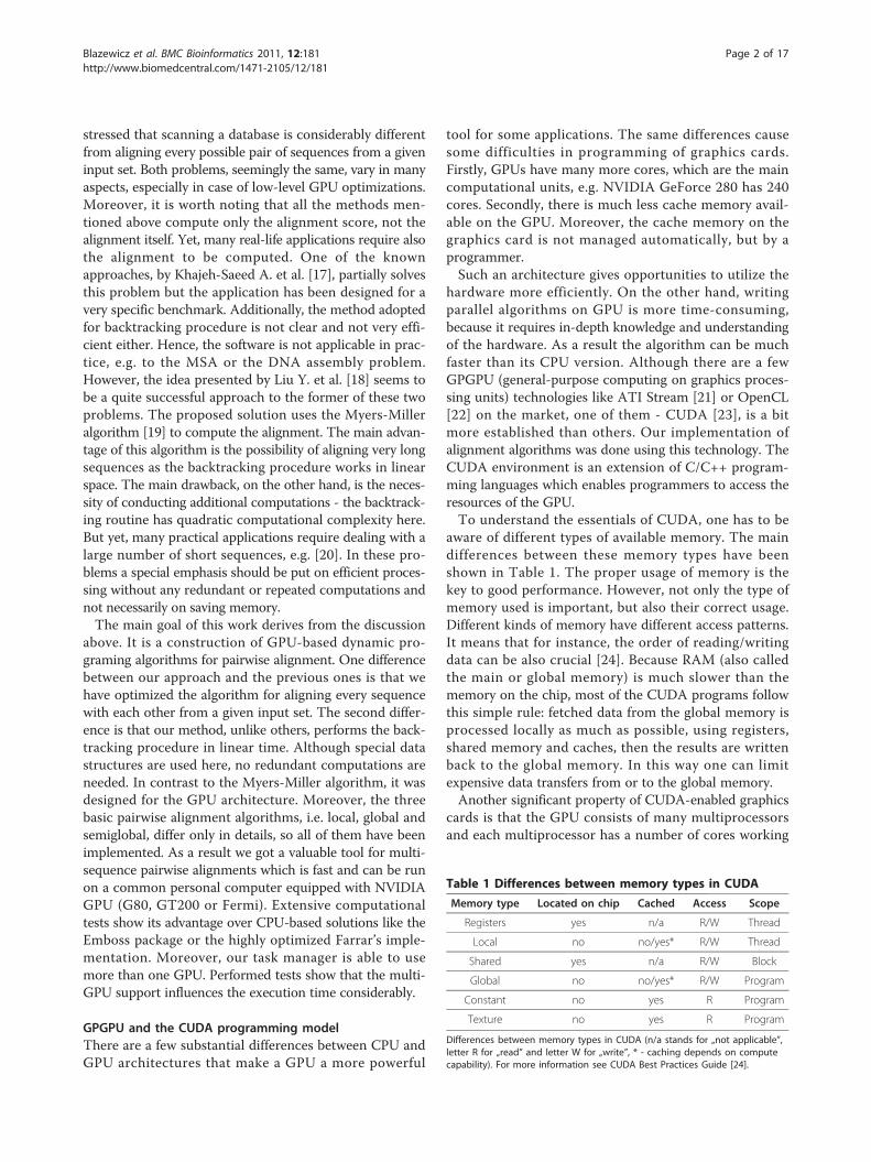
aware of different types of available memory. The maindifferences between these memory types have beenshown in Table 1. The proper usage of memory is thekey to good performance. However, not only the type ofmemory used is important, but also their correct usage.Different kinds of memory have different access patterns.It means that for instance, the order of reading/writingdata can be also crucial [24]. Because RAM (also calledthe main or global memory) is much slower than thememory on the chip, most of the CUDA programs followthis simple rule: fetched data from the global memory isprocessed locally as much as possible, using registers,shared memory and caches, then the results are writtenback to the global memory. In this way one can limitexpensive data transfers from or to the global memory.Another significant property of CUDA-enabled graphics

cards is that the GPU consists of many multiprocessorsand each multiprocessor has a number of cores working

Table 1 Differences between memory types in CUDA

Memory type Located on chip Cached Access Scope

Registers yes n/a R/W Thread

Local no no/yes* R/W Thread

Shared yes n/a R/W Block

Global no no/yes* R/W Program

Constant no yes R Program

Texture no yes R Program

Differences between memory types in CUDA (n/a stands for „not applicable”,letter R for „read” and letter W for „write”, * - caching depends on computecapability). For more information see CUDA Best Practices Guide [24].


of 17

as one or more SIMT (single instruction multiple thread)units. One such unit is able to execute one and only oneinstruction at the same time, but in many threads and onvarious parts of data. As a result, during the process ofdesigning an algorithm, one must take this intoconsideration.Being conscious of the architecture described briefly

above, one can design and implement alignment algo-rithms efficiently.

Algorithms for pairwise sequence alignmentThere are three basic algorithms for performing pairwisesequence alignment: Needleman-Wunsch [1] for com-puting global alignment, its modification for semiglobalalignment and Smith-Waterman [2] for computing localalignment. All these algorithms are based on the idea ofdynamic programming and to some extent work analo-gically. Taking into consideration Gotoh’s enhancement[25], the algorithms are described briefly below.Let us define:

• A - a set of characters of nucleic acids or proteins,• si - the i-th sequence,• si(k) Î A - k-th character of the i-th sequence,• SM - substitution matrix,• SM(ci Î A, cj Î A) - substitution score for ci and cjpair,• Gopen - penalty for opening a gap,• Gext - penalty for extending a gap,• H - a matrix with partial alignment scores,• E - a matrix with partial alignment scores indicat-ing vertical gap continuation,• F - a matrix with partial alignment scores indicat-ing horizontal gap continuation,

Needleman-Wunsch algorithmTo compute the alignment of two sequences, the algo-rithm (called later NW algorithm) has to fill the matrixH according to the similarity function. The similarityfunction determines a score of substitution between tworesidues. This relation is given in a substitution matrix,like one from BLOSUM [26] or PAM [27] families. Thematrix H also takes gap penalties into account,described by Gopen and Gext. The size of the matrix H is(n + 1) × (m + 1), where n is the number of residues inthe first sequence s1 and m - in the second sequence s2.The matrix H is filled using the following formulae:

Hi,j = max

⎧⎪⎨⎪⎩

Ei,j

Fi,j

Hi−1,j−1 + SM(s1(i), s2(j))

⎫⎪⎬⎪⎭ (1)

Ei,j = max{

Ei,j−1 − Gext

Hi,j−1 − Gopen

}(2)

Fi,j = max{

Fi−1,j − Gext

Hi−1,j − Gopen

}(3)

where i = 1...n and j = 1...m.The first row and the first column are filled according

to the following formulae:

Hi,0 = −i · Gext − Gopen (4)

H0,j = −j · Gext − Gopen (5)

Moreover, the E and F matrices are initialized by put-ting -∞ value into the first row and column. The resultfor this part of the algorithm is the value of similarity,so called score. Let us denote the coordinates of the cellwith the similarity score by (i*, j*). In case of the NWalgorithm, this value can be found in the H(n, m) cell ofthe matrix H.The goal of the second stage - backtracking, is to

retrieve the final alignment of two sequences. The ideaof backtracking is that the algorithm performs backwardmoves starting from the (i*, j*) cell in the matrix H untilit reaches the (0, 0) cell. Every time when the algorithmmoves to the upper cell, a gap character is inserted intothe sequence s1 in the final alignment. If the algorithmmoves left, a gap is added analogically to the sequences2, and finally the diagonal move means that the corre-sponding residues are aligned. The backtracking proce-dure is deeply analyzed in Section “The idea ofbacktracking procedure and GPU limitations”.The semiglobal pairwise alignmentA semiglobal version of dynamic programming for pair-wise alignment differs from the previous one in threepoints. The first one is the way how the matrix H isinitialized. For semiglobal alignment the formulae (4)and (5) should be replaced respectively by:

Hi,0 = 0 (6)

H0,j = 0 (7)

The second difference concerns the coordinates of thecell where the similarity score can be found in thematrix H. For semiglobal alignment this cell is the onewith the highest value from the last row or column ofthe matrix H.The last difference involves the stop criterion for the

backtracking procedure. In this case backtracking is fin-ished when the cell (k, 0) or (0, l) is reached, where k =0, ..., n and l = 0, ..., m.Smith-Waterman algorithm for the local pairwise alignmentThe Smith-Waterman algorithm (called later SW algo-rithm) also differs from the Needleman-Wunsch algo-rithm in three points. The first one is again the way ofinitializing the matrix H. The initializing values should


of 17

be the same as in the semiglobal version of thealgorithm.The second difference concerns the formulae describ-

ing the process of filling the matrix H. The formula (1)should be replaced by the following one:

Hi,j = max

⎧⎪⎪⎨⎪⎪⎩

0Ei,j

Fi,j

Hi−1,j−1 + SM(s1(i), s2(j))

⎫⎪⎪⎬⎪⎪⎭ (8)

where i = 1...n and j = 1...m.The next difference covers the coordinates of the cell

with the final score for the local alignment. In this casethe (i*, j*) cell is the one with the highest value withinthe entire matrix H.The last difference concerns the stop criterion of the

backtracking procedure. The Smith-Waterman algo-rithm is finished when a cell with zero value is reached.

ImplementationThe idea of backtracking procedure and GPU limitationsTo obtain the alignment efficiently four booleanmatrices have been defined in our approach, each ofsize (n + 1) × (m + 1). The purpose of these matrices isto indicate the proper direction of backward moves forthe algorithm being at a certain position during the pro-cess of backtracking. Although their memory usage isquadratic, the advantage is that they enable to performthe backtracking procedure in a linear time, in contrastto the Mayers and Miller’s idea.The backtracking matrices are defined as follows:

• Cup - indicates whether the algorithm should con-tinue moving up,• Cleft - indicates whether the algorithm should con-tinue moving left,• Bup - indicates whether the algorithm should moveup, if it does not continue its way up or left,• Bleft - indicates whether the algorithm should moveleft, if it does not continue its way up or left.

Two special cases should be stressed:

• if Cup = false, Cleft = false, Bup = true and Bleft =true then the algorithm should move to the diagonalcell in the up left direction,• if Cup, Cleft, Bup and Bleft have logical value falsethen the backtracking procedure is finished.

In the case of global and semiglobal alignment algo-rithms, the matrices are filled according to the followingformulae:

Cupi,j =

{true if Ei,j = Ei,j−1 − Gext

false else(9)

Clefti,j =

{true if Fi,j = Fi−1,j − Gext

false else(10)

Bupi,j =

⎧⎨⎩

true if Hi,j = Ei,j orHi,j = SM(s1(i), s2(j)) + Hi−1,j−1

false else(11)

Blefti,j =

⎧⎨⎩

true if (Hi,j = Fi,j and Hi,j �= Ei,j) orHi,j = SM(s1(i), s2(j)) + Hi−1,j−1

false else(12)

The additional condition of Hi,j ≠ Ei,j in the formula(12), as compared to the formula (11), prevents the algo-rithm from an ambiguous situation, when both direc-tions, up and left, are equally good. In this case, toavoid non-deterministic behavior, the algorithm shouldprefer only one, predefined direction.For the local alignment algorithm, the Cup and Cleft

matrices are filled according to formulae (9) and (10),respectively. However, the Bup and Bleft matrices arefilled using the following formulae:

Bupi,j =

⎧⎪⎪⎨⎪⎪⎩

true if(Hi,j = Ei,j orHi,j = SM(s1(i), s2(j)) + Hi−1,j−1) andHi,j > 0

false else

(13)

Blefti,j =

⎧⎪⎪⎨⎪⎪⎩

true if((Hi,j = Fi,j and Hi,j �= Ei,j) orHi,j = SM(s1(i), s2(j)) + Hi−1,j−1) and

Hi,j > 0false else

(14)

An important issue, one should take into considera-tion, is that during the process of filling the matrix Hany cell value can be computed only if the values of theleft, above and diagonal cells are known. It means thatonly these cells that are on the same anti-diagonal canbe processed simultaneously. As a result, there is notmuch to parallelize (in the context of massively parallelGPU architecture) in a single run of NW or SW algo-rithm. However, progressive multiple sequence align-ment algorithms require aligning of many sequences(every sequence with each other). Our idea was todesign an algorithm for efficient execution of many pair-wise alignment instances running concurrently. To uti-lize the GPU resources properly one has to load it witha sufficient amount of work. To fulfill this requirementat least 80 × 80 NW/SW instances should be computedconcurrently (this number will be explained in Section“Implementation of the algorithms”). The problem to


of 17

overcome was that the amount of available RAM ongraphics cards was, for this purpose, relatively small (e.g.the GeForce GTX 280 usually has 1 GB of RAM). Infact, the H, E and F matrices do not have to be keptentirely in RAM (see Section “Implementation of thealgorithms”). However, the backtracking tables (Cup,Cleft, Bup, Bleft) must be kept in the global memory.Hence, they would take a lot of memory space if theywere held in normal C/C++ boolean arrays, e.g. forsequences with lengths of 500 residues one would need80 × 80 × 5002 × 4 bytes i.e. 6103.5 MB only for back-tracking arrays. Thus, a special emphasis has been putto make this figure smaller, so that the algorithm can berun on any CUDA-capable device.

Implementation of the algorithmsAll the algorithms in our implementation, namely theNW algorithm, its semiglobal version and the SW algo-rithm, have a few input parameters such as a substitu-tion matrix, Gopen and Gext values, a file in fasta formatwith sequences to be aligned, etc. When the algorithmis launched, it performs an alignment of every givensequence with each other. The result of the algorithmconsists of the score and the alignment for each pair ofsequences.Let S be the set of input sequences. The total number

N of sequences’ pairs to be aligned is given by the fol-lowing formula:

N =| S |(| S | − 1)

2(15)

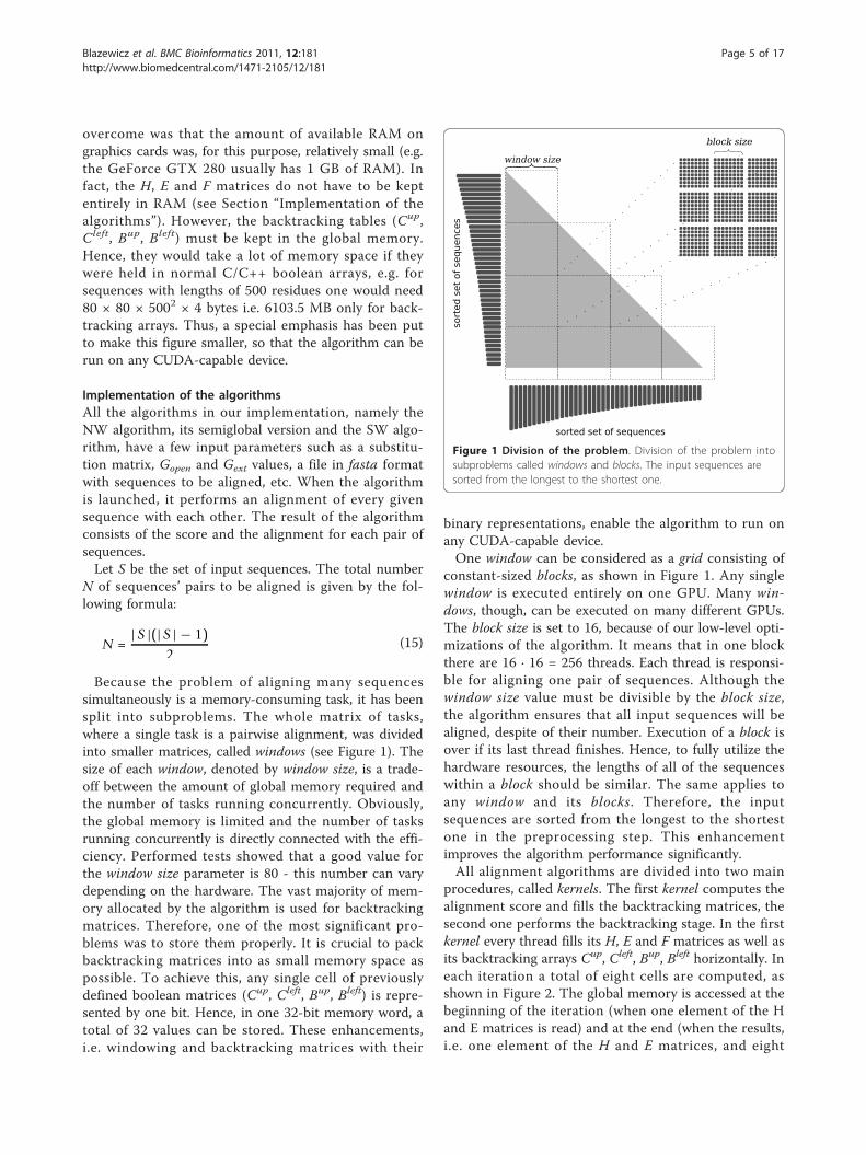
Because the problem of aligning many sequencessimultaneously is a memory-consuming task, it has beensplit into subproblems. The whole matrix of tasks,where a single task is a pairwise alignment, was dividedinto smaller matrices, called windows (see Figure 1). Thesize of each window, denoted by window size, is a trade-off between the amount of global memory required andthe number of tasks running concurrently. Obviously,the global memory is limited and the number of tasksrunning concurrently is directly connected with the effi-ciency. Performed tests showed that a good value forthe window size parameter is 80 - this number can varydepending on the hardware. The vast majority of mem-ory allocated by the algorithm is used for backtrackingmatrices. Therefore, one of the most significant pro-blems was to store them properly. It is crucial to packbacktracking matrices into as small memory space aspossible. To achieve this, any single cell of previouslydefined boolean matrices (Cup, Cleft, Bup, Bleft) is repre-sented by one bit. Hence, in one 32-bit memory word, atotal of 32 values can be stored. These enhancements,i.e. windowing and backtracking matrices with their

binary representations, enable the algorithm to run onany CUDA-capable device.One window can be considered as a grid consisting of

constant-sized blocks, as shown in Figure 1. Any singlewindow is executed entirely on one GPU. Many win-dows, though, can be executed on many different GPUs.The block size is set to 16, because of our low-level opti-mizations of the algorithm. It means that in one blockthere are 16 · 16 = 256 threads. Each thread is responsi-ble for aligning one pair of sequences. Although thewindow size value must be divisible by the block size,the algorithm ensures that all input sequences will bealigned, despite of their number. Execution of a block isover if its last thread finishes. Hence, to fully utilize thehardware resources, the lengths of all of the sequenceswithin a block should be similar. The same applies toany window and its blocks. Therefore, the inputsequences are sorted from the longest to the shortestone in the preprocessing step. This enhancementimproves the algorithm performance significantly.All alignment algorithms are divided into two main

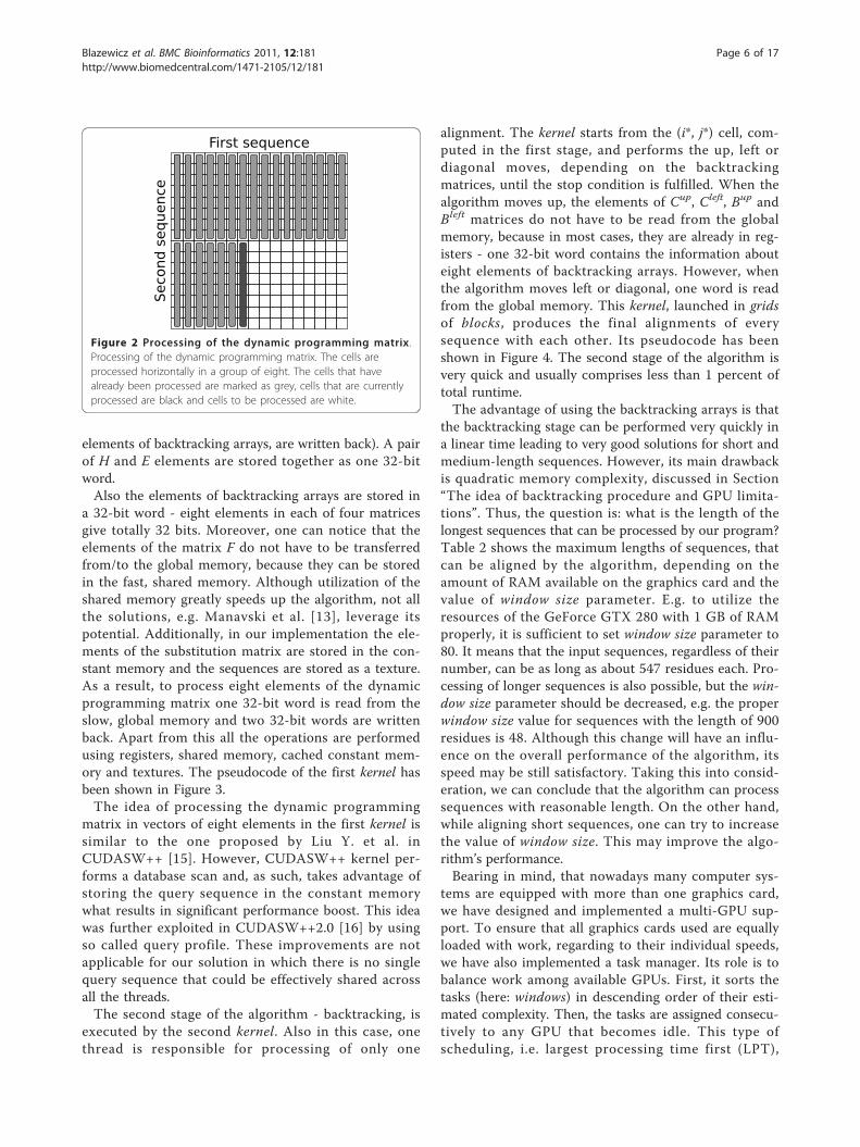
procedures, called kernels. The first kernel computes thealignment score and fills the backtracking matrices, thesecond one performs the backtracking stage. In the firstkernel every thread fills its H, E and F matrices as well asits backtracking arrays Cup, Cleft, Bup, Bleft horizontally. Ineach iteration a total of eight cells are computed, asshown in Figure 2. The global memory is accessed at thebeginning of the iteration (when one element of the Hand E matrices is read) and at the end (when the results,i.e. one element of the H and E matrices, and eight

Figure 1 Division of the problem. Division of the problem intosubproblems called windows and blocks. The input sequences aresorted from the longest to the shortest one.


of 17

elements of backtracking arrays, are written back). A pairof H and E elements are stored together as one 32-bitword.Also the elements of backtracking arrays are stored in

a 32-bit word - eight elements in each of four matricesgive totally 32 bits. Moreover, one can notice that theelements of the matrix F do not have to be transferredfrom/to the global memory, because they can be storedin the fast, shared memory. Although utilization of theshared memory greatly speeds up the algorithm, not allthe solutions, e.g. Manavski et al. [13], leverage itspotential. Additionally, in our implementation the ele-ments of the substitution matrix are stored in the con-stant memory and the sequences are stored as a texture.As a result, to process eight elements of the dynamicprogramming matrix one 32-bit word is read from theslow, global memory and two 32-bit words are writtenback. Apart from this all the operations are performedusing registers, shared memory, cached constant mem-ory and textures. The pseudocode of the first kernel hasbeen shown in Figure 3.The idea of processing the dynamic programming

matrix in vectors of eight elements in the first kernel issimilar to the one proposed by Liu Y. et al. inCUDASW++ [15]. However, CUDASW++ kernel per-forms a database scan and, as such, takes advantage ofstoring the query sequence in the constant memorywhat results in significant performance boost. This ideawas further exploited in CUDASW++2.0 [16] by usingso called query profile. These improvements are notapplicable for our solution in which there is no singlequery sequence that could be effectively shared acrossall the threads.The second stage of the algorithm - backtracking, is

executed by the second kernel. Also in this case, onethread is responsible for processing of only one

alignment. The kernel starts from the (i*, j*) cell, com-puted in the first stage, and performs the up, left ordiagonal moves, depending on the backtrackingmatrices, until the stop condition is fulfilled. When thealgorithm moves up, the elements of Cup, Cleft, Bup andBleft matrices do not have to be read from the globalmemory, because in most cases, they are already in reg-isters - one 32-bit word contains the information abouteight elements of backtracking arrays. However, whenthe algorithm moves left or diagonal, one word is readfrom the global memory. This kernel, launched in gridsof blocks, produces the final alignments of everysequence with each other. Its pseudocode has beenshown in Figure 4. The second stage of the algorithm isvery quick and usually comprises less than 1 percent oftotal runtime.The advantage of using the backtracking arrays is that

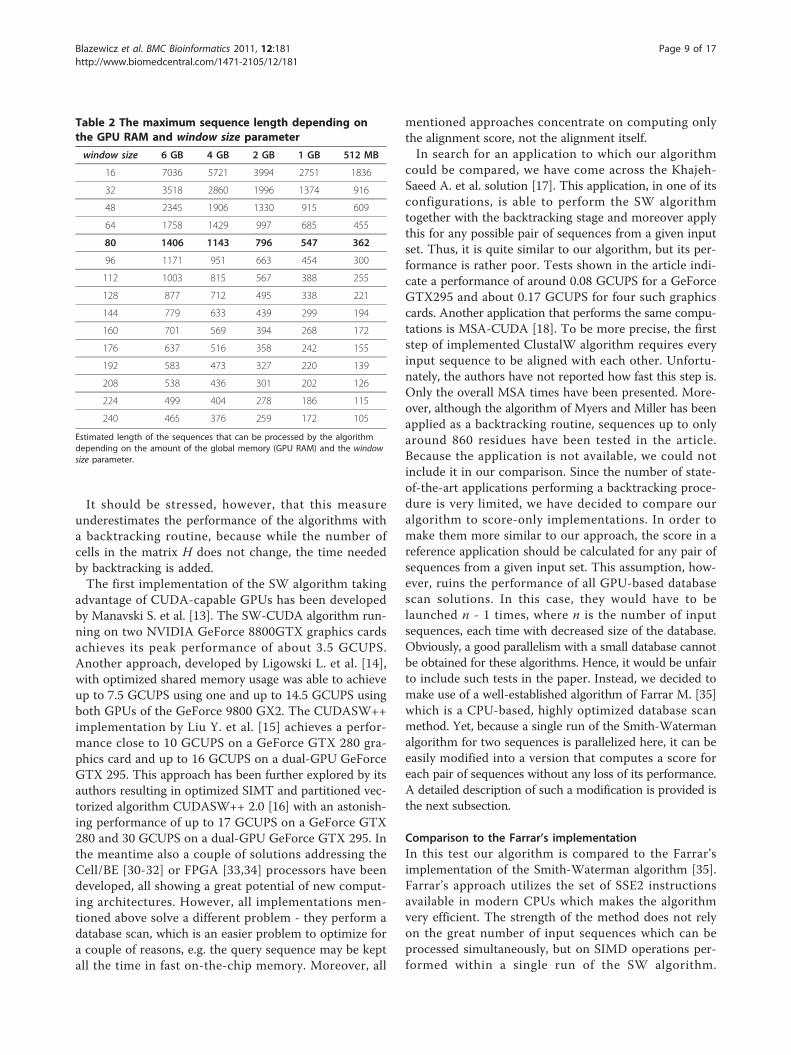
the backtracking stage can be performed very quickly ina linear time leading to very good solutions for short andmedium-length sequences. However, its main drawbackis quadratic memory complexity, discussed in Section“The idea of backtracking procedure and GPU limita-tions”. Thus, the question is: what is the length of thelongest sequences that can be processed by our program?Table 2 shows the maximum lengths of sequences, thatcan be aligned by the algorithm, depending on theamount of RAM available on the graphics card and thevalue of window size parameter. E.g. to utilize theresources of the GeForce GTX 280 with 1 GB of RAMproperly, it is sufficient to set window size parameter to80. It means that the input sequences, regardless of theirnumber, can be as long as about 547 residues each. Pro-cessing of longer sequences is also possible, but the win-dow size parameter should be decreased, e.g. the properwindow size value for sequences with the length of 900residues is 48. Although this change will have an influ-ence on the overall performance of the algorithm, itsspeed may be still satisfactory. Taking this into consid-eration, we can conclude that the algorithm can processsequences with reasonable length. On the other hand,while aligning short sequences, one can try to increasethe value of window size. This may improve the algo-rithm’s performance.Bearing in mind, that nowadays many computer sys-

tems are equipped with more than one graphics card,we have designed and implemented a multi-GPU sup-port. To ensure that all graphics cards used are equallyloaded with work, regarding to their individual speeds,we have also implemented a task manager. Its role is tobalance work among available GPUs. First, it sorts thetasks (here: windows) in descending order of their esti-mated complexity. Then, the tasks are assigned consecu-tively to any GPU that becomes idle. This type ofscheduling, i.e. largest processing time first (LPT),

Figure 2 Processing of the dynamic programming matrix.Processing of the dynamic programming matrix. The cells areprocessed horizontally in a group of eight. The cells that havealready been processed are marked as grey, cells that are currentlyprocessed are black and cells to be processed are white.


of 17

although not optimal, ensures that the upper bound of

execution time is equal to (43

− 13m

) · topt, where topt is

the optimal execution time and m - number of proces-sing units [28,29]. In practice, applying LPT rule resultsin very good run times.

ResultsThe main goal of this section is to compare the perfor-mance of the algorithm to other state-of-the-artapproaches. However, before proceeding to the actualtests, the measure of cell updates per second (CUPS)should be well understood. The measure represents the

//--->

for (x = 0; x < sequenceX.length; x++)

{H up = readFromGlobal(x); F up = readFromGlobal(x);

sequenceXElement = readFromTexture(x);

H upleft = H init; H init = H up;

unsigned int back = 0;

// |

// V

for(i = 0; i < 8; i++)

{H left = readFromShared(i); E left = readFromShared(i);

sequenceYElement = readFromShared(i);

//reading value of substitution matrix from constant memory

similarity = readFromConstant(sequenceXElement, sequenceYElement);

E current = max(E left - gapEx, H left - gapOp);

F current = max(F up - gapEx, H up - gapOp);

H current = max(E current, F current);

H current = max(H current, H upleft + similarity);

//backtracking arrays

back <<= 1;

back |= (H_current == F current) ||

(H_current == H upleft + similarity); //if go up

back <<= 1;

back |= (H_current == E current) &&

(H_current != F current) ||

(H_current == H upleft + similarity); //if go left

back <<= 1;

back |= F_current == F up - gapEx; //if continue up

back <<= 1;

back |= E_current == E left - gapEx; //if continue left

//initialize variables for next iteration

writeToShared(H current, i); writeToShared(E current, i);

H upleft = H left; H up = H current; F up = F current;

}writeToGlobal(H up,x); writeToGlobal(F up,x); writeToGlobal(back,x,y);

}Figure 3 Pseudocode of the first kernel. Pseudocode of the inner loops in the first kernel. The H matrix is filled in a way specific to the NWalgorithm.


of 17

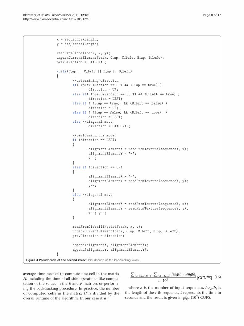
average time needed to compute one cell in the matrixH, including the time of all side operations like compu-tation of the values in the E and F matrices or perform-ing the backtracking procedure. In practice, the numberof computed cells in the matrix H is divided by theoverall runtime of the algorithm. In our case it is:

∑i∈{1,2,...,n−1}

∑j∈{1,2,...,i} lengthi · lengthj

t · 109 [GCUPS] (16)

where n is the number of input sequences, lengthi isthe length of the i-th sequence, t represents the time inseconds and the result is given in giga (109) CUPS.

x = sequecnceXLength;

y = sequecnceYLength;

readFromGlobal(back, x, y);

unpackCurrentElement(back, C up, C left, B up, B left);

prevDirection = DIAGONAL;

while(C up || C left || B up || B left)

{//determining direction

if( (prevDirection == UP) && (C up == true) )

direction = UP;

else if( (prevDirection == LEFT) && (C left == true) )

direction = LEFT;

else if ( (B up == true) && (B left == false) )

direction = UP;

else if ( (B up == false) && (B left == true) )

direction = LEFT;

else //diagonal move

direction = DIAGONAL;

//performing the move

if (direction == LEFT)

{alignmentElementX = readFromTexture(sequenceX, x);

alignmentElementY = ’-’;

x--;

}else if (direction == UP)

{alignmentElementX = ’-’;

alignmentElementY = readFromTexture(sequenceY, y);

y--;

}else //diagonal move

{alignmentElementX = readFromTexture(sequenceX, x);

alignmentElementY = readFromTexture(sequenceY, y);

x--; y--;

}

readFromGlobalIfNeeded(back, x, y);

unpackCurrentElement(back, C up, C left, B up, B left);

prevDirection = direction;

append(alignmentX, alignmentElementX);

append(alignmentY, alignmentElementY);

}Figure 4 Pseudocode of the second kernel. Pseudocode of the backtracking kernel.


of 17

It should be stressed, however, that this measureunderestimates the performance of the algorithms witha backtracking routine, because while the number ofcells in the matrix H does not change, the time neededby backtracking is added.The first implementation of the SW algorithm taking

advantage of CUDA-capable GPUs has been developedby Manavski S. et al. [13]. The SW-CUDA algorithm run-ning on two NVIDIA GeForce 8800GTX graphics cardsachieves its peak performance of about 3.5 GCUPS.Another approach, developed by Ligowski L. et al. [14],with optimized shared memory usage was able to achieveup to 7.5 GCUPS using one and up to 14.5 GCUPS usingboth GPUs of the GeForce 9800 GX2. The CUDASW++implementation by Liu Y. et al. [15] achieves a perfor-mance close to 10 GCUPS on a GeForce GTX 280 gra-phics card and up to 16 GCUPS on a dual-GPU GeForceGTX 295. This approach has been further explored by itsauthors resulting in optimized SIMT and partitioned vec-torized algorithm CUDASW++ 2.0 [16] with an astonish-ing performance of up to 17 GCUPS on a GeForce GTX280 and 30 GCUPS on a dual-GPU GeForce GTX 295. Inthe meantime also a couple of solutions addressing theCell/BE [30-32] or FPGA [33,34] processors have beendeveloped, all showing a great potential of new comput-ing architectures. However, all implementations men-tioned above solve a different problem - they perform adatabase scan, which is an easier problem to optimize fora couple of reasons, e.g. the query sequence may be keptall the time in fast on-the-chip memory. Moreover, all

mentioned approaches concentrate on computing onlythe alignment score, not the alignment itself.In search for an application to which our algorithm

could be compared, we have come across the Khajeh-Saeed A. et al. solution [17]. This application, in one of itsconfigurations, is able to perform the SW algorithmtogether with the backtracking stage and moreover applythis for any possible pair of sequences from a given inputset. Thus, it is quite similar to our algorithm, but its per-formance is rather poor. Tests shown in the article indi-cate a performance of around 0.08 GCUPS for a GeForceGTX295 and about 0.17 GCUPS for four such graphicscards. Another application that performs the same compu-tations is MSA-CUDA [18]. To be more precise, the firststep of implemented ClustalW algorithm requires everyinput sequence to be aligned with each other. Unfortu-nately, the authors have not reported how fast this step is.Only the overall MSA times have been presented. More-over, although the algorithm of Myers and Miller has beenapplied as a backtracking routine, sequences up to onlyaround 860 residues have been tested in the article.Because the application is not available, we could notinclude it in our comparison. Since the number of state-of-the-art applications performing a backtracking proce-dure is very limited, we have decided to compare ouralgorithm to score-only implementations. In order tomake them more similar to our approach, the score in areference application should be calculated for any pair ofsequences from a given input set. This assumption, how-ever, ruins the performance of all GPU-based databasescan solutions. In this case, they would have to belaunched n - 1 times, where n is the number of inputsequences, each time with decreased size of the database.Obviously, a good parallelism with a small database cannotbe obtained for these algorithms. Hence, it would be unfairto include such tests in the paper. Instead, we decided tomake use of a well-established algorithm of Farrar M. [35]which is a CPU-based, highly optimized database scanmethod. Yet, because a single run of the Smith-Watermanalgorithm for two sequences is parallelized here, it can beeasily modified into a version that computes a score foreach pair of sequences without any loss of its performance.A detailed description of such a modification is provided isthe next subsection.

Comparison to the Farrar’s implementationIn this test our algorithm is compared to the Farrar’simplementation of the Smith-Waterman algorithm [35].Farrar’s approach utilizes the set of SSE2 instructionsavailable in modern CPUs which makes the algorithmvery efficient. The strength of the method does not relyon the great number of input sequences which can beprocessed simultaneously, but on SIMD operations per-formed within a single run of the SW algorithm.

Table 2 The maximum sequence length depending onthe GPU RAM and window size parameter

window size 6 GB 4 GB 2 GB 1 GB 512 MB

16 7036 5721 3994 2751 1836

32 3518 2860 1996 1374 916

48 2345 1906 1330 915 609

64 1758 1429 997 685 455

80 1406 1143 796 547 362

96 1171 951 663 454 300

112 1003 815 567 388 255

128 877 712 495 338 221

144 779 633 439 299 194

160 701 569 394 268 172

176 637 516 358 242 155

192 583 473 327 220 139

208 538 436 301 202 126

224 499 404 278 186 115

240 465 376 259 172 105

Estimated length of the sequences that can be processed by the algorithmdepending on the amount of the global memory (GPU RAM) and the windowsize parameter.


of 17

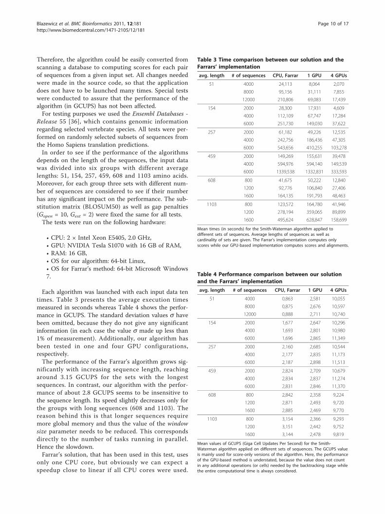
Therefore, the algorithm could be easily converted fromscanning a database to computing scores for each pairof sequences from a given input set. All changes neededwere made in the source code, so that the applicationdoes not have to be launched many times. Special testswere conducted to assure that the performance of thealgorithm (in GCUPS) has not been affected.For testing purposes we used the Ensembl Databases -

Release 55 [36], which contains genomic informationregarding selected vertebrate species. All tests were per-formed on randomly selected subsets of sequences fromthe Homo Sapiens translation predictions.In order to see if the performance of the algorithms

depends on the length of the sequences, the input datawas divided into six groups with different averagelengths: 51, 154, 257, 459, 608 and 1103 amino acids.Moreover, for each group three sets with different num-ber of sequences are considered to see if their numberhas any significant impact on the performance. The sub-stitution matrix (BLOSUM50) as well as gap penalties(Gopen = 10, Gext = 2) were fixed the same for all tests.The tests were run on the following hardware:

• CPU: 2 × Intel Xeon E5405, 2.0 GHz,• GPU: NVIDIA Tesla S1070 with 16 GB of RAM,• RAM: 16 GB,• OS for our algorithm: 64-bit Linux,• OS for Farrar’s method: 64-bit Microsoft Windows7.

Each algorithm was launched with each input data tentimes. Table 3 presents the average execution timesmeasured in seconds whereas Table 4 shows the perfor-mance in GCUPS. The standard deviation values s havebeen omitted, because they do not give any significantinformation (in each case the value s made up less than1% of measurement). Additionally, our algorithm hasbeen tested in one and four GPU configurations,respectively.The performance of the Farrar’s algorithm grows sig-

nificantly with increasing sequence length, reachingaround 3.15 GCUPS for the sets with the longestsequences. In contrast, our algorithm with the perfor-mance of about 2.8 GCUPS seems to be insensitive tothe sequence length. Its speed slightly decreases only forthe groups with long sequences (608 and 1103). Thereason behind this is that longer sequences requiremore global memory and thus the value of the windowsize parameter needs to be reduced. This correspondsdirectly to the number of tasks running in parallel.Hence the slowdown.Farrar’s solution, that has been used in this test, uses

only one CPU core, but obviously we can expect aspeedup close to linear if all CPU cores were used.

Table 3 Time comparison between our solution and theFarrars’ implementation

avg. length # of sequences CPU, Farrar 1 GPU 4 GPUs

51 4000 24,113 8,064 2,070

8000 95,156 31,111 7,855

12000 210,806 69,083 17,439

154 2000 28,300 17,931 4,609

4000 112,109 67,747 17,284

6000 251,730 149,030 37,622

257 2000 61,182 49,226 12,535

4000 242,756 186,436 47,305

6000 543,656 410,255 103,278

459 2000 149,269 155,631 39,478

4000 594,976 594,140 149,539

6000 1339,538 1332,831 333,593

608 800 41,675 50,222 12,840

1200 92,776 106,840 27,406

1600 164,135 191,793 48,463

1103 800 123,572 164,780 41,946

1200 278,194 359,065 89,899

1600 495,624 628,847 158,699

Mean times (in seconds) for the Smith-Waterman algorithm applied todifferent sets of sequences. Average lengths of sequences as well ascardinality of sets are given. The Farrar’s implementation computes onlyscores while our GPU-based implementation computes scores and alignments.

Table 4 Performance comparison between our solutionand the Farrars’ implementation

avg. length # of sequences CPU, Farrar 1 GPU 4 GPUs

51 4000 0,863 2,581 10,055

8000 0,875 2,676 10,597

12000 0,888 2,711 10,740

154 2000 1,677 2,647 10,296

4000 1,693 2,801 10,980

6000 1,696 2,865 11,349

257 2000 2,160 2,685 10,544

4000 2,177 2,835 11,173

6000 2,187 2,898 11,513

459 2000 2,824 2,709 10,679

4000 2,834 2,837 11,274

6000 2,831 2,846 11,370

608 800 2,842 2,358 9,224

1200 2,871 2,493 9,720

1600 2,885 2,469 9,770

1103 800 3,154 2,366 9,293

1200 3,151 2,442 9,752

1600 3,144 2,478 9,819

Mean values of GCUPS (Giga Cell Updates Per Second) for the Smith-Waterman algorithm applied on different sets of sequences. The GCUPS valueis mainly used for score-only versions of the algorithm. Here, the performanceof the GPU-based method is understated, because the value does not countin any additional operations (or cells) needed by the backtracking stage whilethe entire computational time is always considered.


of 17

However, our approach is also scalable - the executiontimes drop by a factor of nearly four when all fourGPUs are used and the algorithm reaches up to 11.5GCUPS. The number of input sequences does not affectthe performance of Farrar’s approach and it was highenough to have no influence on the performance of ouralgorithm. We can conclude that for sequences of aver-age length (459) both implementations run comparablyfast, but the GPU-based algorithm tends to be much fas-ter when short sequences are processed. Moreover, it isworth noting that our algorithm additionally performsthe backtracking step and computes the actual align-ments of the sequences.The speedup is much higher if the algorithm is com-

pared to the one presented by Khajeh-Saeed A. et al. in[17]. Up to our knowledge this is the only GPU-basedsolution addressing the same problem where the perfor-mance is reported. Our approach is about 35 and 68times faster for one and four graphics cards, respectively.

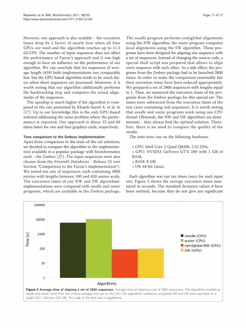
Time comparison to the Emboss implementationApart from comparison to the state-of-the-art solutions,we decided to compare the algorithm to the implementa-tion available in a popular package with bioinformaticstools - the Emboss [37]. The input sequences were alsochosen from the Ensembl Databases - Release 55 (seeSection “Comparison to the Farrar’s implementation”).We tested ten sets of sequences, each containing 2800entries with lengths between 100 and 420 amino acids.The execution times of our NW and SW algorithms’implementations were compared with needle and waterprograms, which are available in the Emboss package.

The needle program performs semiglobal alignmentsusing the NW algorithm, the water program computeslocal alignments using the SW algorithm. These pro-grams have been designed for aligning one sequence witha set of sequences. Instead of changing the source code, aspecial shell script was prepared that allows to alignevery sequence with each other. As a side effect, the pro-grams from the Emboss package had to be launched 2800times. In order to make the comparison reasonably fairtheir execution times have been reduced appropriately.We prepared a set of 2800 sequences with lengths equalto 1. Then, we measured the execution times of the pro-grams from the Emboss package for this special set. Thetimes were subtracted from the execution times of thetest cases containing real sequences. It is worth notingthat needle and water programs work using one CPUthread. Obviously, the NW and SW algorithms are deter-ministic - they always find the optimal solution. There-fore, there is no need to compare the quality of theresults.The tests were run on the following hardware:

• CPU: Intel Core 2 Quad Q8200, 2.33 GHz,• GPU: NVIDIA GeForce GTX 280 with 1 GB ofRAM,• RAM: 8 GB,• OS: 64-bit Linux.

Each algorithm was run ten times (once for each inputset). Figure 5 shows the average execution times mea-sured in seconds. The standard deviation values s havebeen omitted, because they do not give any significant

Figure 5 Average time of aligning a set of 2800 sequences. Average time of aligning a set of 2800 sequences. The algorithms marked asneedle and water come from the Emboss package and ran on the CPU. The algorithms marked as semiglobal NW and SW were launched on asingle GPU - GeForce GTX 280. The scale of the time axis is logarithmic.


of 17

information (in each case the value s comprised lessthan 1% of the measure).The average times of computation for the needle and

water programs were 6157 and 10957 seconds respec-tively (about 102 and 182 minutes), whereas the timesfor our implementation were as follows: 89.7 secondsfor the NW and 100.8 seconds for the SW algorithm.Thus, the GPU implementation of the semiglobal ver-sion of NW was about 68 times faster than the CPU-based needle. In case of the SW algorithm the differencewas even higher: the GPU version was about 108 timesfaster. To show this relationship properly, the scale ofthe time axis in Figure 5 is logarithmic.

Multi-GPU testThe multi-GPU test was performed to see how the timeof the computations depends on the number of graphicscards used. The sets of input sequences were the sameas in the case of the test from Section “Comparison tothe Farrar’s implementation”.The tests were run on the following hardware:

• CPU: 2 × Intel Xeon E5405, 2.0 GHz,• GPU: NVIDIA Tesla S1070 with 16 GB of RAM,• RAM: 16 GB,• OS: 64-bit Linux.

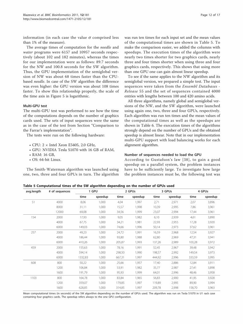
The Smith-Waterman algorithm was launched usingone, two, three and four GPUs in turn. The algorithm

was run ten times for each input set and the mean valuesof the computational times are shown in Table 5. Tomake the comparison easier, we added the columns withspeedups. The execution times of the algorithm werenearly two times shorter for two graphics cards, nearlythree and four times shorter when using three and fourgraphics cards, respectively. This shows that using morethan one GPU one can gain almost linear speedup.To see if the same applies to the NW algorithm and its

semiglobal version, we prepared a simple test. The inputsequences were taken from the Ensembl Databases -Release 55 and the set of sequences contained 4000entries with lengths between 100 and 420 amino acids.All three algorithms, namely global and semiglobal ver-

sions of the NW, and the SW algorithm, were launchedusing again one, two, three and four GPUs, respectively.Each algorithm was run ten times and the mean values ofthe computational times as well as the speedups areshown in Table 6. The execution times of the algorithmsstrongly depend on the number of GPUs and the obtainedspeedup is almost linear. Note that in our implementationmulti-GPU support with load balancing works for eachalignment algorithm.

Number of sequences needed to load the GPUAccording to Gustafson ’s law [38], to gain a goodspeedup on a parallel system, the problem instanceshave to be sufficiently large. To investigate how largethe problem instances must be, the following test was

Table 5 Computational times of the SW algorithm depending on the number of GPUs used

avg.length # of sequences 1 GPU 2 GPUs 3 GPUs 4 GPUs

time speedup time speedup time speedup time speedup

51 4000 8,06 1,000 4,04 1,997 2,71 2,971 2,07 3,896

8000 31,11 1,000 15,57 1,998 10,39 2,995 7,86 3,961

12000 69,08 1,000 34,56 1,999 23,07 2,994 17,44 3,961

154 2000 17,93 1,000 9,05 1,982 6,10 2,939 4,61 3,890

4000 67,75 1,000 34,21 1,981 22,93 2,955 17,28 3,920

6000 149,03 1,000 74,66 1,996 50,14 2,973 37,62 3,961

257 2000 49,23 1,000 24,72 1,991 16,59 2,968 12,54 3,927

4000 186,44 1,000 93,80 1,988 62,80 2,969 47,31 3,941

6000 410,26 1,000 205,87 1,993 137,26 2,989 103,28 3,972

459 2000 155,63 1,000 78,16 1,991 52,45 2,967 39,48 3,942

4000 594,14 1,000 298,50 1,990 198,57 2,992 149,54 3,973

6000 1332,83 1,000 667,31 1,997 444,92 2,996 333,59 3,995

608 800 50,22 1,000 25,66 1,957 17,40 2,886 12,84 3,911

1200 106,84 1,000 53,91 1,982 35,77 2,987 27,41 3,898

1600 191,79 1,000 95,93 1,999 64,01 2,996 48,46 3,958

1103 800 164,78 1,000 83,84 1,965 56,83 2,900 41,95 3,928

1200 359,07 1,000 179,85 1,997 119,89 2,995 89,90 3,994

1600 628,85 1,000 314,85 1,997 209,78 2,998 158,70 3,963

Mean computational times (in seconds) of the SW algorithm depending on the number of GPUs used. The algorithm was run on Tesla S1070 in U1 rack casecontaining four graphics cards. The speedup refers always to the one GPU configuration.


of 17

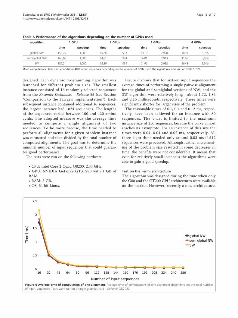
designed. Each dynamic programming algorithm waslaunched for different problem sizes. The smallestinstance consisted of 16 randomly selected sequencesfrom the Ensembl Databases - Release 55 (see Section“Comparison to the Farrar’s implementation”). Eachsubsequent instance contained additional 16 sequences,the largest instance had 1024 sequences. The lengthsof the sequences varied between 100 and 420 aminoacids. The adopted measure was the average timeneeded to compute a single alignment of twosequences. To be more precise, the time needed toperform all alignments for a given problem instancewas measured and then divided by the total number ofcomputed alignments. The goal was to determine theminimal number of input sequences that could guaran-tee good performance.The tests were run on the following hardware:

• CPU: Intel Core 2 Quad Q8200, 2.33 GHz,• GPU: NVIDIA GeForce GTX 280 with 1 GB ofRAM,• RAM: 8 GB,• OS: 64-bit Linux.

Figure 6 shows that for sixteen input sequences theaverage times of performing a single pairwise alignmentfor the global and semiglobal versions of NW, and theSW algorithm were relatively long - about 1.72, 1.84and 2.15 milliseconds, respectively. These times weresignificantly shorter for larger sizes of the problem.The reasonable times of 0.1, 0.1 and 0.12 ms, respec-

tively, have been achieved for an instance with 80sequences. The chart is limited to the maximuminstance size of 256 sequences, because the curve almostreaches its asymptote. For an instance of this size thetimes were 0.04, 0.04 and 0.05 ms, respectively. Allthree algorithms needed only around 0.03 ms if 512sequences were processed. Although further increment-ing of the problem size resulted in some decreases intime, the benefits were not considerable. It means thateven for relatively small instances the algorithms wereable to gain a good speedup.

Test on the Fermi architectureThe algorithm was designed during the time when onlythe G80 and the GT200 GPU architectures were availableon the market. However, recently a new architecture,

Table 6 Performance of the algorithms depending on the number of GPUs used

algorithm 1 GPU 2 GPUs 3 GPUs 4 GPUs

time speedup time speedup time speedup time speedup

global NW 158,25 1,000 81,86 1,933 54,19 2,920 40,41 3,916

semiglobal NW 163,16 1,000 84,81 1,924 56,01 2,913 41,69 3,914

SW 182,01 1,000 93,89 1,939 61,96 2,938 46,48 3,916

Mean computational times (in seconds) for 4000 input sequences depending on the number of GPUs used. The algorithms were run on Tesla S1070.

Figure 6 Average time of computation of one alignment. Average time of computations of one alignment depending on the total numberof input sequences. Tests were run on a single graphics card - GeForce GTX 280.


of 17

called Fermi [39], has come along. Hence, we set out tocheck if the application can benefit from a doubled num-ber of CUDA cores that are on the new chips.The sets of input sequences were the same as in the case

of the test from Section “Comparison to the Farrar’simplementation”. Only the longest sequences wereexcluded, because of more limited memory on the gra-phics cards.The tests were run on the following hardware:

• CPU: Intel Core i7 950, 3.06 GHz,• GPU: 2× NVIDIA GeForce GTX 480 with 1.5 GBof RAM,• RAM: 8 GB,• OS: 64-bit Linux.

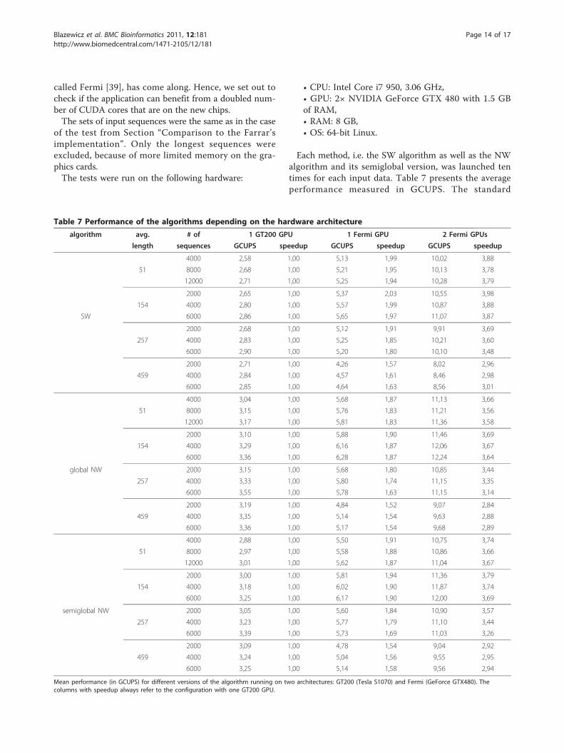
Each method, i.e. the SW algorithm as well as the NWalgorithm and its semiglobal version, was launched tentimes for each input data. Table 7 presents the averageperformance measured in GCUPS. The standard

Table 7 Performance of the algorithms depending on the hardware architecture

algorithm avg. # of 1 GT200 GPU 1 Fermi GPU 2 Fermi GPUs

length sequences GCUPS speedup GCUPS speedup GCUPS speedup

4000 2,58 1,00 5,13 1,99 10,02 3,88

51 8000 2,68 1,00 5,21 1,95 10,13 3,78

12000 2,71 1,00 5,25 1,94 10,28 3,79

2000 2,65 1,00 5,37 2,03 10,55 3,98

154 4000 2,80 1,00 5,57 1,99 10,87 3,88

SW 6000 2,86 1,00 5,65 1,97 11,07 3,87

2000 2,68 1,00 5,12 1,91 9,91 3,69

257 4000 2,83 1,00 5,25 1,85 10,21 3,60

6000 2,90 1,00 5,20 1,80 10,10 3,48

2000 2,71 1,00 4,26 1,57 8,02 2,96

459 4000 2,84 1,00 4,57 1,61 8,46 2,98

6000 2,85 1,00 4,64 1,63 8,56 3,01

4000 3,04 1,00 5,68 1,87 11,13 3,66

51 8000 3,15 1,00 5,76 1,83 11,21 3,56

12000 3,17 1,00 5,81 1,83 11,36 3,58

2000 3,10 1,00 5,88 1,90 11,46 3,69

154 4000 3,29 1,00 6,16 1,87 12,06 3,67

6000 3,36 1,00 6,28 1,87 12,24 3,64

global NW 2000 3,15 1,00 5,68 1,80 10,85 3,44

257 4000 3,33 1,00 5,80 1,74 11,15 3,35

6000 3,55 1,00 5,78 1,63 11,15 3,14

2000 3,19 1,00 4,84 1,52 9,07 2,84

459 4000 3,35 1,00 5,14 1,54 9,63 2,88

6000 3,36 1,00 5,17 1,54 9,68 2,89

4000 2,88 1,00 5,50 1,91 10,75 3,74

51 8000 2,97 1,00 5,58 1,88 10,86 3,66

12000 3,01 1,00 5,62 1,87 11,04 3,67

2000 3,00 1,00 5,81 1,94 11,36 3,79

154 4000 3,18 1,00 6,02 1,90 11,87 3,74

6000 3,25 1,00 6,17 1,90 12,00 3,69

semiglobal NW 2000 3,05 1,00 5,60 1,84 10,90 3,57

257 4000 3,23 1,00 5,77 1,79 11,10 3,44

6000 3,39 1,00 5,73 1,69 11,03 3,26

2000 3,09 1,00 4,78 1,54 9,04 2,92

459 4000 3,24 1,00 5,04 1,56 9,55 2,95

6000 3,25 1,00 5,14 1,58 9,56 2,94

Mean performance (in GCUPS) for different versions of the algorithm running on two architectures: GT200 (Tesla S1070) and Fermi (GeForce GTX480). Thecolumns with speedup always refer to the configuration with one GT200 GPU.


of 17

deviation values s were insignificant (less than 1% ofmeasurement) and hence omitted. Additionally, thetable includes the performance of the previous genera-tion architecture - GT200, represented here by oneGPU from the Tesla S1070 (see Section “Comparison tothe Farrar’s implementation”).The test shows that with the Fermi architecture the

performance of the algorithms increases by a factor ofnearly two, especially for short sequences. In case oflonger sequences this dominance is slightly reduced,because only 1.5 GB of RAM was available on ourFermi graphics card whereas one Tesla has 4 GB.Obviously, Fermi GPU with 3 or 6 GB of memory maysolve this performance issue. However, one shouldremember that the solution aims to process mainlyshort and medium-length sequences.

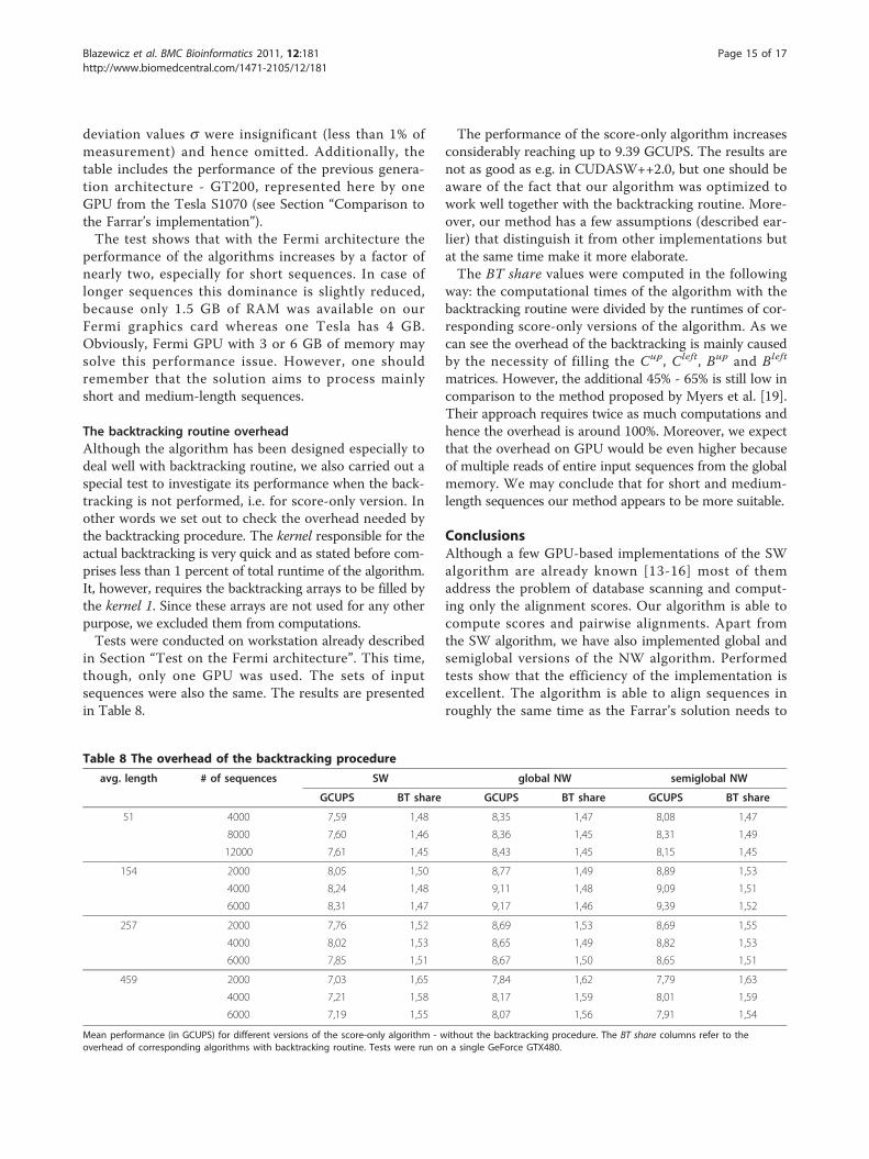
The backtracking routine overheadAlthough the algorithm has been designed especially todeal well with backtracking routine, we also carried out aspecial test to investigate its performance when the back-tracking is not performed, i.e. for score-only version. Inother words we set out to check the overhead needed bythe backtracking procedure. The kernel responsible for theactual backtracking is very quick and as stated before com-prises less than 1 percent of total runtime of the algorithm.It, however, requires the backtracking arrays to be filled bythe kernel 1. Since these arrays are not used for any otherpurpose, we excluded them from computations.Tests were conducted on workstation already described

in Section “Test on the Fermi architecture”. This time,though, only one GPU was used. The sets of inputsequences were also the same. The results are presentedin Table 8.

The performance of the score-only algorithm increasesconsiderably reaching up to 9.39 GCUPS. The results arenot as good as e.g. in CUDASW++2.0, but one should beaware of the fact that our algorithm was optimized towork well together with the backtracking routine. More-over, our method has a few assumptions (described ear-lier) that distinguish it from other implementations butat the same time make it more elaborate.The BT share values were computed in the following

way: the computational times of the algorithm with thebacktracking routine were divided by the runtimes of cor-responding score-only versions of the algorithm. As wecan see the overhead of the backtracking is mainly causedby the necessity of filling the Cup, Cleft, Bup and Bleft

matrices. However, the additional 45% - 65% is still low incomparison to the method proposed by Myers et al. [19].Their approach requires twice as much computations andhence the overhead is around 100%. Moreover, we expectthat the overhead on GPU would be even higher becauseof multiple reads of entire input sequences from the globalmemory. We may conclude that for short and medium-length sequences our method appears to be more suitable.

ConclusionsAlthough a few GPU-based implementations of the SWalgorithm are already known [13-16] most of themaddress the problem of database scanning and comput-ing only the alignment scores. Our algorithm is able tocompute scores and pairwise alignments. Apart fromthe SW algorithm, we have also implemented global andsemiglobal versions of the NW algorithm. Performedtests show that the efficiency of the implementation isexcellent. The algorithm is able to align sequences inroughly the same time as the Farrar’s solution needs to

Table 8 The overhead of the backtracking procedure

avg. length # of sequences SW global NW semiglobal NW

GCUPS BT share GCUPS BT share GCUPS BT share

51 4000 7,59 1,48 8,35 1,47 8,08 1,47

8000 7,60 1,46 8,36 1,45 8,31 1,49

12000 7,61 1,45 8,43 1,45 8,15 1,45

154 2000 8,05 1,50 8,77 1,49 8,89 1,53

4000 8,24 1,48 9,11 1,48 9,09 1,51

6000 8,31 1,47 9,17 1,46 9,39 1,52

257 2000 7,76 1,52 8,69 1,53 8,69 1,55

4000 8,02 1,53 8,65 1,49 8,82 1,53

6000 7,85 1,51 8,67 1,50 8,65 1,51

459 2000 7,03 1,65 7,84 1,62 7,79 1,63

4000 7,21 1,58 8,17 1,59 8,01 1,59

6000 7,19 1,55 8,07 1,56 7,91 1,54

Mean performance (in GCUPS) for different versions of the score-only algorithm - without the backtracking procedure. The BT share columns refer to theoverhead of corresponding algorithms with backtracking routine. Tests were run on a single GeForce GTX480.


of 17

compute only scores. Yet, its real dominance revealswhile short sequences are processed with no perfor-mance loss. Moreover, the speed of our GPU-basedalgorithms can be almost linearly increased when usingmore than one graphics card. We have also checkedwhat is a minimum reasonable number of inputsequences. Performed tests show, that even for about 80sequences our algorithms are able to gain a goodspeedup. What is worth noting, all the tests were per-formed using real sequences.The NW and SW algorithms with a backtracking rou-

tine may have a lot of applications. They can be used as arobust method for multi-pairwise sequence comparisonsperformed during the first step in all of the multiplesequence alignment methods based on the progressiveapproach. Another area of interest can be the usage of aGPU-based semiglobal alignment procedure as a part ofthe algorithm for the DNA assembly problem, being oneof the most challenging problem in current biological stu-dies. It has already been shown that in this case a parallelsolution can be successfully applied [20]. Using GPU-based approaches we expect that its execution time wouldbe even shorter, because the large number of shortsequences is perfectly in line with the benefits of ouralgorithm.

Availability and requirements• Project name: gpu-pairAlign• Project home page: http://gpualign.cs.put.poznan.pl• Operating system: Linux• Programming language: C/C++• Other requirements: CUDA 2.0 or higher, CUDAcompliant GPU, make, g++• License: GNU GPLv3• Any restrictions to use by non-academics: none

AbbreviationsNW: the Needleman-Wunsch algorithm; SW: the Smith-Waterman algorithm;CPU: central processing unit; GPU: graphics processing unit; GPGPU: general-purpose computing on graphics processing units; CUDA: Compute UnifiedDevice Architecture; RAM: random access memory; OS: operating system.

AcknowledgementsThis research has been partially supported by the Polish Ministry of Scienceand Higher Education under Grant No. N N519 314635.

Author details1Poznań University of Technology, Poznań, Poland. 2Institute of BioorganicChemistry PAS, Poznań, Poland. 3University of Siegen, Siegen, Germany.4Poznań Supercomputing and Networking Center, Poznań, Poland.

Authors’ contributionsWF, MK and PW conceived of the study and participated in its design. WFproposed the idea of backtracking arrays. WF and MK contributed equally toalgorithm design and implementation. MK carried out computational tests.JB and EP participated in the coordination of the project. All authors wereinvolved in writing the manuscript and all of them read and approved itsfinal version.

Received: 30 December 2010 Accepted: 20 May 2011Published: 20 May 2011

References1. Needlemana S, Wunsch C: A general method applicable to the search for

similarities in the amino acid sequence of two proteins. J Mol Biol 1970,48(3):443-3, 48: 443-53.

2. Smith T, Waterman M: Identification of Common MolecularSubsequences. Journal of Molecular Biology 1981, 147:195-97.

3. Deonier R, Tavare C, Waterman M: Computational Genome Analysis. Springer2005.

4. Pevzner P: Computational Molecular Biology: An Algorithmic Approach. TheMIT Press 2000.

5. Blazewicz J, Bryja M, Figlerowicz M, Gawron P, Kasprzak M, Kirton E, Platt D,Przybytek J, Swiercz A, Szajkowski L: Whole genome assembly from 454sequencing output via modified DNA graph concept. ComputationalBiology and Chemistry 2009, 33:224-230.

6. Wang L, Jiang T: On the complexity of multiple sequence alignment.J Comput Biol 1994, 1(4):337-348.

7. Pei J: Multiple protein sequence alignment. Current Opinion in StructuralBiology 2008, 18(3):382-386.

8. Do CB, Mahabhashyam MS, Brudno M, Batzoglou S: ProbCons: Probabilisticconsistency-based multiple sequence alignment. Genome Res 2005,15(2):330-340.

9. Lassmann T, Sonnhammer EL: Kalign - an accurate and fast multiplesequence alignment algorithm. BMC Bioinformatics 2005, 6:298 [http://www.biomedcentral.com/1471-2105/6/298].

10. Thompson J, Higgins D, Gibson T: CLUSTAL W: improving the sensitivityof progressivemultiple sequence alignment through sequenceweighting, position-specific gap penalties and weight matrix choice.Nucleic Acids Research 1994, 22:4673-4680.

11. Notredame C, Higgins D, Heringa J: T-Coffee: A novel method for multiplesequence alignments. Journal of Molecular Biology 2000, 302:205-217.

12. Kemena C, Notredame C: Upcoming challenges for multiple sequencealignment methods in the high-throughput era. Bioinformatics 2009,25(19):2455-2465.

13. Manavski S, Valle G: CUDA compatible GPU cards as efficient hardwareaccelerators for Smith-Waterman sequence alignment. BMC Bioinformatics2008, 9.

14. Ligowski L, Rudnicki W: An efficient implementation of Smith Watermanalgorithm on GPU using CUDA, for massively parallel scanning ofsequence databases. IPDPS 2009, 1-9.

15. Liu Y, Maskell DL, Schmidt B: CUDASW++: optimizing Smith-Watermansequence database searches for CUDA-enabled graphics processingunits. BMC Research Notes 2009, 2.

16. Liu Y, Maskell DL, Schmidt B: CUDASW++2.0: enhanced Smith-Watermanprotein database search on CUDA-enabled GPUs based on SIMT andvirtualized SIMD abstractions. BMC Research Notes 2010, 3.

17. Khajeh-Saeed A, Poole S, Perot J: Acceleration of the Smith-Watermanalgorithm using single and multiple graphics processors. Journal ofComputational Physics 2010, 229:4247-4258.

18. Liu Y, Maskell DL, Schmidt B: MSA-CUDA: Multiple Sequence Alignmenton Graphics Processing Units with CUDA. 20th IEEE InternationalConference on Application-specific Systems, Architectures and Processors 2009.

19. Myers EW, Miller W: Optimal alignments in linear space. Comput ApplBiosci 1988, 4:11-17.

20. Blazewicz J, Kasprzak M, Swiercz A, Figlerowicz M, Gawron P, Platt D,Szajkowski L: Parallel Implementation of the Novel Approach to GenomeAssembly. Proc SNPD 2008, IEEE Computer Society 2008, 732-737.

21. ATI Stream. [http://www.amd.com/stream].22. OpenCL. [http://www.khronos.org/opencl].23. NVIDIA CUDA. [http://www.nvidia.com/object/cuda_home.html].24. NVIDIA CUDA C Programming Best Practices Guide. [http://www.nvidia.

com/object/cuda_develop.html].25. Gotoh O: An Improved Algorithm for Matching Biological Sequences.

Journal of Molecular Biology 1981, 162:705-708.26. Henikoff S, Henikoff J: Amino Acid Substitution Matrices from Protein

Blocks. PNAS 1992, 89:10915-10919.27. Dayhoff M, Schwartz R, Orcutt B: A model of Evolutionary Change in

Proteins. Atlas of protein sequence and structure, Nat Biomed Res Found1978, 5(supp 3):345-58.


of 17

http://gpualign.cs.put.poznan.pl

http://www.ncbi.nlm.nih.gov/pubmed/5420325?dopt=Abstract












http://www.biomedcentral.com/1471-2105/6/298

http://www.biomedcentral.com/1471-2105/6/298









http://www.amd.com/stream

http://www.khronos.org/opencl

http://www.nvidia.com/object/cuda_home.html

http://www.nvidia.com/object/cuda_develop.html

http://www.nvidia.com/object/cuda_develop.html



28. Graham RL: Bounds on multiprocessing timing anomalies. SIAM J ApplMath 1969, 17(2):416-429.

29. Blazewicz J, Ecker K, Pesch E, Schmidt G, Weglarz J: Handbook onScheduling: From Theory to Applications. Springer 2007.

30. Szalkowski A, Ledergerber C, Krahenbuhl P, C D: SWPS3 - fast multi-threaded vectorized Smith-Waterman for IBM Cell/B.E. and x86/SSE2.BMC Research Notes 2008, 107.

31. Farrar M: Optimizing Smith-Waterman for the Cell Broad-band Engine.[http://farrar.michael.googlepages.com/SW-CellBE.pdf].

32. Wirawan A, Kwoh C, Hieu N, Schmidt B: CBESW: Sequence Alignment onPlaystation 3. BMC Bioinformatics 2008, 9:377.

33. Oliver T, Schmidt B, DL M: Reconfigurable architectures for bio-sequencedatabase scanning on FPGAs. IEEE Trans Circuit Syst II 2005, 52:851-55.

34. Li T, Shum W, Truong K: 160-fold acceleration of the Smith-Watermanalgorithm using a field programmable gate array (FPGA). BMCBioinformatics 2007, 8:185.

35. Farrar M: Striped Smith-Waterman speeds database searches six timesover other SIMD implementations. Bioinformatics 2007, 23(2):156-161.

36. Ensembl Databases - Release 55. [ftp://ftp.ensembl.org/pub/release-55].37. Rice P, Longden I, Bleasby A: EMBOSS: The European Molecular Biology

Open Software Suite. Trends in Genetics 2000, 16:276-77.38. Gustafson J: Reevaluating Amdahl’s Law. Communications of the ACM

1988, 31:532-533.39. NVIDIA Fermi Architecture. [http://www.nvidia.com/object/

Fermi_architecture.html].

doi:10.1186/1471-2105-12-181Cite this article as: Blazewicz et al.: Protein alignment algorithms withan efficient backtracking routine on multiple GPUs. BMC Bioinformatics2011 12:181.

Submit your next manuscript to BioMed Centraland take full advantage of:

• Convenient online submission

• Thorough peer review

• No space constraints or color figure charges

• Immediate publication on acceptance

• Inclusion in PubMed, CAS, Scopus and Google Scholar

• Research which is freely available for redistribution

Submit your manuscript at www.biomedcentral.com/submit


of 17

http://farrar.michael.googlepages.com/SW-CellBE.pdf







ftp://ftp.ensembl.org/pub/release-55



http://www.nvidia.com/object/Fermi_architecture.html

http://www.nvidia.com/object/Fermi_architecture.html

protein alignment algorithms with an efficient backtracking routine on multiple gpus

Documents