protection technolo protective systems for high-voltage

Protection Technology"Protective systems for high-voltage transmission lines"

Equipment Description Part Number

Adjustable Three-Phase Power Supply

(0 - 400V/2A, 72PU)

3301-3ZT

(ST8008-4S7)

Three Phase Power Quality Meter with display and long-term memory CO5127-1S

Circuit breaker

(Power-Switch Module)CO3301-5P

Transmission line model CO3301-3A

Resistive load CO3301-3F

Equipmentnt

Overcurrent time protection relay CO3301-4J

Multimeter

Protective device in a branch

Background/Introduction

Public electricity networks place very high demands on the protection technology needed to guarantee secure and uninterrupted energy supply. Protective mechanisms are needed to monitor electrical networks and equipment. Electrical faults must be quickly identified and treated to minimize damage to equipment. A protective device's relay evaluates the measurement variables comprising current and voltage as well as their combinations, and disconnects the affected line section by means of a circuit breaker in the event of a malfunction. As an example, for a protective relay to come into action, it must be energized (excited) beforehand. The excitation modes can comprise overcurrent, undervoltage, or impedance. The measured variables are supplied to the protective relay via transformers. A protective device accordingly encompasses the associated protective relay as well as the equipment necessary for measuring and switching. Low-maintenance systems with high selectivity, speed and interrupting capacity are required to perform the tasks above, so that the fusible cut-outs normally found in low-voltage systems no longer prove practical. The selectivity just mentioned is achieved, for example, via a measurement variable, time grading or a reference measurement, so that only the affected network section is identified and deactivated in the event of a malfunction.

As mentioned above, a protective relay is only one part of a protective device, whose main elements can be exemplified by a branch (Figure 1). The sequence here ranges from the busbar (1) through elements like the circuit breaker (3) to the outgoing feeder (7). Two disconnectors (2) enclose the circuit breaker to establish a visible isolating distance for maintenance tasks or coupling procedures. The earthing switch (5) is used to connect the outgoing feeder (7) in the released state to an earth potential so as not to endanger maintenance personnel. Branches can be realized as feed couplers or outgoing feeders.

1. Busbar2. Disconnector3. Circuit breaker4. Current transformer5. Earthing switch6. Voltage transformer7. Outgoing feeder

Figure 1:Branch

The busbars, branches, switching devices and measuring elements together make up the switchgear, whose definition is as follows: Switchgear is the combination of switching devices, associated closed/open-loop control, measurement and protective mechanisms, assembly groups comprising such devices and mechanisms; as well as the related connections, accessories, enclosures and supporting structures. In the broadest sense, the purpose of switchgear is to connect, interrupt and disconnect current paths. This permits measures such as dependable control of electrical energy flows, quickest possible remedy of malfunctions, as well as maintenance and repair services.

In the case of switchgear, a distinction is always made between primary and secondary systems. Elements such as busbars, isolators, circuit breakers and outgoing feeders form part of the primary system. This is accompanied by secondary systems comprising all auxiliary equipment such as those required for measurement, remote control, monitoring and protection. The main components are described further below:

Disconnectors

Disconnectors (off-load switch) serve for visible isolation of current paths. They are often installed before and behind a circuit breaker to ensure, for example, clearly identifiable separation through visual contact for maintenance purposes. Disconnectors must only be operated off-load, and are therefore mechanically interlocked in switchgear, hence only operable once the associated circuit breaker has been tripped (disconnectors are not included in the experiment setup).

Circuit Breakers

Circuit breakers are used to energize and de-energize electrical equipment, consumers, or even entire segments of a facility. In addition to switching operating currents, circuit breakers are able to switch high powers such as those occurring during short circuits. Circuit breakers in medium and high voltage networks differ in terms of their quenching principle according to the voltage levels involved, and in terms of their insulation medium. In the medium-voltage range, vacuum is finding increasingly widespread use as the quenching agent. Sulphur hexafluoride (SF6) is also used as a quenching agent, but more commonly in the high-voltage range. The insulation medium is the surrounding area between the switch and the outer housing. Air or sulphur hexafluoride (SF6) again is commonly used here, depending on requirements.

Transformers

Depending on requirements, switchgear also contains current and voltage transformers. If non-directional overcurrent time protection has been realized in the system, for instance, a use of current transformers normally proves sufficient. If distance protection has been realized, voltage transformers are needed additionally to calculate impedance. Transformers are used to adjust operating voltages and currents to manageable levels so that they are useful for measurement devices without damaging them. A distinction is made here between instrument transformers and protective transformers. The instrument ones have a high accuracy in the nominal operating range but cannot withstand short-circuit currents. In contrast, protective transformers can withstand high short circuit currents, but are less inaccurate. Transformers operate on the principle of induction and capacitive decoupling.

Earthing Switches

Earthing switches are integrated into certain segments of a facility to ensure that these segments remain de-energized following disconnection of the supply voltage. The induced voltages often occurring in an absence of such switches can be hazardous, especially for people (earthing switches are not included in the experiment setup).

Choice of protective device

The total duration of a switch-off operation starting with fault occurrence and ending with fault remedy followed by restoration of the protective device to operational readiness comprises a number of individual phases which represented as shown below (Figure 2).

After an operating time starting on occurrence of a fault, the relay is energized. A trip command is issued after the command time. The circuit breaker is then tripped. However, the relay contact opens mechanically only after an opening time has elapsed. If the short-circuit involves the occurrence of an electric arc, the short circuit ends on electrical opening of the contact following quenching. The excitation drops off and the relay returns to its initial state.

Figure 2: Time phases of Switching Operation

1. Overcurrent Time Protection.2. Directional Overcurrent Time Protection.3. Overvoltage and Undervoltage Protection.4. Directional Power Protection.5. Earth Fault Protection.6. Parallel Line Protection.7. High Speed Distance Protection.

The type of protection depends on the voltage level, networks nature and neutral point handling. Also of relevance to protection of lines (underground cables / overhead lines) are the transmission distance and type. In high voltage networks with low resistance, neutral-point earthing, single-pole and three-pole short circuits are detected and shut off by the same protective device. In medium voltage, short range networks, use is made of an isolated neutral point. Single-pole short circuits here are usually self-extinguishing. In this case, the protective device should only detect long-term earth faults, e.g.. using a related protective mechanism. Multi-pole short circuits require very short switch-off times in all cases.

Overcurrent time protection is adequate for simple radial networks operating at medium-voltages. Directional overcurrent protection, distance protection or differential protection are needed for fulfilling higher protection requirements or for ring networks. Distance protection and differential protection are used to ensure selectivity in meshed networks operating at high and ultra-high voltages. Protective relays are equipped with specific protection techniques depending on the involved application (like generator, transformer, or line protection). Commonly used techniques include:

1.Overcurrent Time Protection

Overcurrent time protection (non-directional overcurrent protection) is a selective type of overload and short-circuit protection used mainly in radial networks with single-ended feed (Figure 3) as found in medium-voltage systems.

Figure 3: Radial network

Most protective devices of this kind also serve as a backup measure for differential and distance protection in the case of transformers, machines and transmission lines. The protective device is energized (excited) by a short circuit current IK or an overcurrent I> which significantly exceeds the operating current IN. To obtain an adequate measurement variable for the protective device, the current is coupled via a current transformer and measured. If the current exceeds the set threshold, this is considered as the start command for the relay's preset time delay. If the excitation is still present after the time delay, the protective device performs the desired action: The output relay is actuated, thereby triggering the circuit breaker. Otherwise, the action is canceled. The reset value at which the protective relay returns to its initial position must be higher than the operating current. This results in a hysteresis defined by the reset ratio R (ratio of release and response values). In modern protective relays, this ratio is approximately R = 0.95 for overcurrent activation. A reset ratio of R = 1 would pose a risk of chatter (uncontrolled engagement and release by the protective device).

Figure 4:

Simple trip characteristic of non-directional, maximum-overcurrent time protection

A disadvantage of the simple trip characteristic is that the delay time is always the same, regardless of the fault current amperage. An excessively long delay time in the event of a fault can result in considerable damage to components. For this reason, most protective devices provide a choice of two or more tripping ranges. Figure 5 shows a distinction between the "overload" and "short circuit" ranges. If the excitation level lies between currents I> and I>>, tripping takes place at instant t> (overload stage). At very high currents beyond I>>, such as those occurring during short circuits, tripping takes place sooner at instant t>> (short-circuit stage).

Simple overcurrent protection is non-directional, i.e. its decision criteria only include the measured current and length of the energized phase. For overcurrent to result in activation, the threshold value must lie below the minimum short-circuit current occurring in the system. Overcurrent time protection can have a directional or non-directional trip characteristic. The single-stage trip characteristic of non-directional, maximum-overcurrent time protection is shown in Figure 4 and functions as described above.

Figure 5:Trip characteristic of two-stage, non-directional, maximum-overcurrent time protection

If several protective devices are connected in series across the network, this leads to a graded curve (Figure 6), the nearest protective relay being tripped in the event of a fault. If a protective relay fails, the previous one acts as a backup with a longer tripping time.

Figure 6: Network map with non-directional, maximum-overcurrent time protection relay

The disadvantage here is that a fault in the vicinity of the feed point, where the tripping time t> is longest, results in the highest current. Consequently, additional protective measures are needed here.

2.Direccional Overcurrent Time Protectionn

Basically, directional overcurrent works like non-directional overcurrent protection. The difference lies in the added ability to detect the direction of energy flow, which permits use in networks with double-ended feed or ring networks (Figure 7). Needed additionally for this purpose is a voltage transformer to determine the phase angle between the current and voltage. Though technically more complex and expensive than radial networks, such systems also guarantee more dependable supply. If a fault occurs in outgoing feeder B, for example, the two surrounding protective devices (marked blue) can isolate this section while all other feeders remain supplied.

Figure 7: Ring Network

A short circuit can result in voltage dips, preventing correct voltage measurements. Serving as help in this case is a reference voltage formed from the two fault-free phases and lagging exactly 90° behind the voltage of the faulty phase. Figure 8 illustrates this with the reference voltage U23 for phase L1.

Figure 8:Response adjustment range

The relay characteristic angle (RCA) can be used to set the direction recognition boundary (blue vector). This angle can be set between 15° and 83° in relation to the reference voltage. If the RCA = 49° (standard setting), a phase angle of -41° (lag) to 139° (lead) between the current and voltage is the decision criterion for the forward direction, any other angle is the decision criterion for the reverse direction.

An overcurrent protection relay can be provided either with a non-directional overcurrent characteristic like the one used in section 1, or a directional characteristic.

Directional, maximum-overcurrent time protection follows a continuous time function t(I) in dependence on the fault current (Figure 9). Every overcurrent value is associated with a fixed delay time. The relay stores several characteristics which can be set via the delay time tI> serving as a multiplier in the case of directional, maximum-overcurrent time protection's trip characteristic. Apart from different time ranges, it is possible to choose between three different characteristics (normal, strong and extremely inverse). Areas of application mainly include overload protection for motors and transformers.

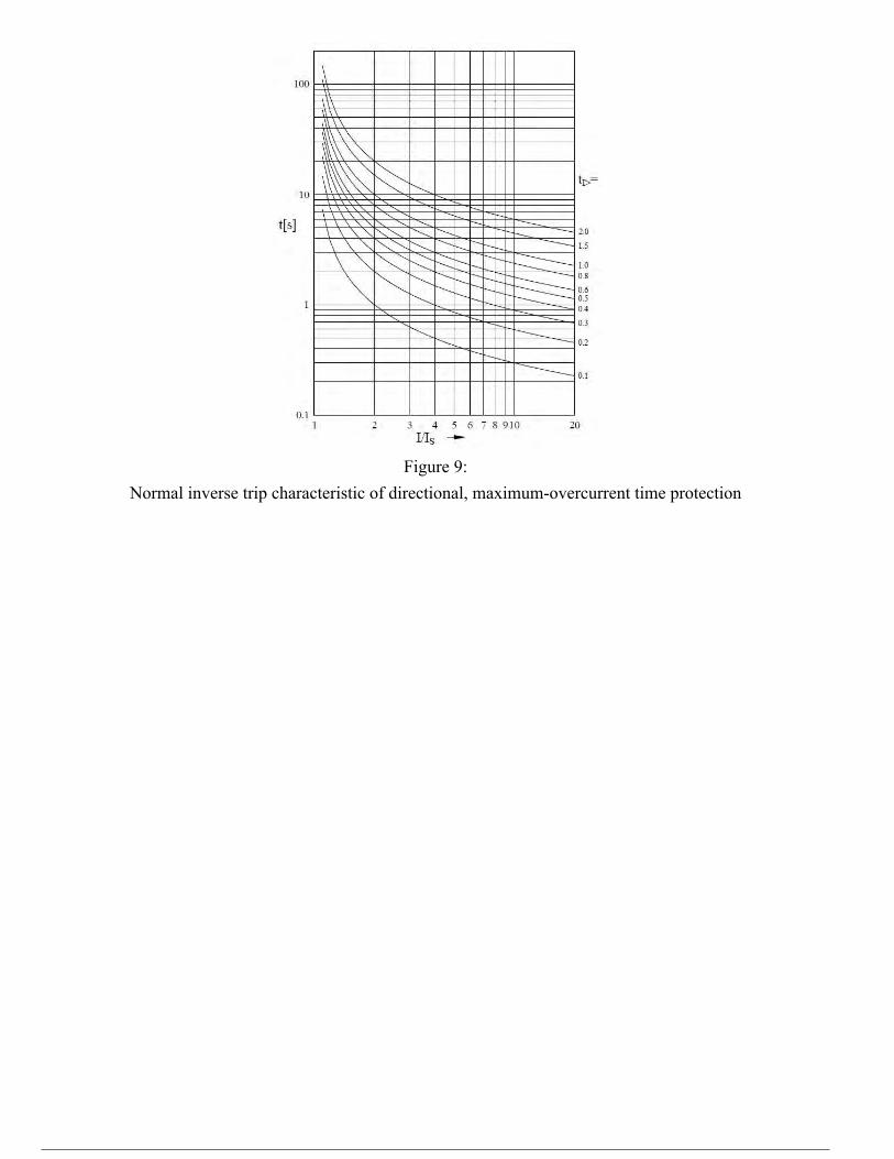
Figure 9:Normal inverse trip characteristic of directional, maximum-overcurrent time protection

3.Overvoltage and Undervoltage Protection

Overvoltage / undervoltage relays - also simply known as voltage relays - are used to monitor the operating voltage of power grids. The voltage is monitored for transgression of certain upper and lower limits. This provides general protection for electricity consumers and generators and as well as other equipment forming part of power transmission systems.

1. Generator2. Protective relay, e.g.. for de-energizing a generatorand/or shutting off a turbine's steam supply.3. Transformer4. Busbar5. Protective relay for disconnecting the motor from thepower grid via a circuit breaker6. Circuit breaker7. Motor

Figure 10:Generator / motor feeder

Unless stated otherwise, the following text uses Figure 10 as orientation and is intended to explain the possible applications of voltage protection relays.

Overvoltage relays (2) are used to protect generators (1) or other equipment such as capacitors. As the load on a generator decreases, its speed and, consequently, voltage increase. Depend on voltage levels, electrical equipment has a certain isolation limit, sometimes defined as the "maximum permissible voltage for equipment" and designated Vm. This voltage is 10 - 15% higher than the nominal or operating voltage (VN). The rated voltage Vr is the voltage corresponding to the equipment's maximum power without any risk of damage during continuous operation.Voltage surge are therefore usually above the rated voltage but not necessarily above the equipment's maximum permissible voltage. The hysteresis here should be less than 20%. This means that after the excitation voltage has dropped off, i.e. the voltage has decreased, the protective relay remains energized by no more than 20% of the excitation voltage before releasing. Figure 11 clarifies this pattern.

Figure 11:

Characteristic with hysteresis

Undervoltage monitoring (5) is performed almost exclusively for motors (7), as they undergo high stresses when their supply voltage is interrupted. In this situation, the motor is disconnected from the power grid network by means of a circuit breaker (6). The pick-up value is about 80% of the nominal voltage. The hysteresis setting for undervoltage should not exceed 17%.

4.Directional Power Protection

Power protection is intended primarily to detect reverse power arising on turbines. During parallel operation of a generator with a network or another generator, it is necessary to monitor the direction of current flow. If the drive turbine fails, the generator operating as a synchronous motor starts to drive the turbine. The protective relay recognizes the reversal of power, immediately after which the generator is disconnected from the power grid network by a circuit breaker. If the fault persists for too long, the drive unit may get damaged. Depending on the fault and the drive unit, switch-off is performed after a delay time of 0 - 30 seconds. If a steam turbine is being used, for instance, action must be taken at an early stage (fast response), only a small percentage of own active power capable of being absorbed. Moreover, a lack of steam causes the turbine to become impermissible hot. The slow response can be set to 10 seconds or longer in the case of fluctuations attributable, for instance, to boiler malfunctions. These protective devices usually have a relatively long release time (e.g.. 500 ms) in order to detect an occurrence of peaks. These peaks are added together during the release time. If the delay time is exceeded within the release time tDO, the device trips again.

Typical settings::

Pick-up values::

Steam turbines:: 1% - 4%

Gas turbines:: 4% - 6%

Diesel generator sets:: 5% - 8%Fast trip stage (e.g.. in the case of load disconnection) 0 s - 3 s

Slow trip stage (e.g.. in the case of boiler malfunction)

10 s - 15 s

In a real application, the relay detects a flow of energy in the forward direction (the current flows from the generator into the line) and the generator is switched off after the trip set time. Likewise when the relay detects reverse power (energy flows to the generator), it's energized and trips immediately. One example of reverse power is failure of a turbine, which would then need to be switched off as soon as possible. In this case, the generator operates as a motor and would damage the turbine. Another characteristic of directional power protection relays is hysteresis (reset ratio) which should be independent from the current tripping value. The minimum hysteresis between the pick-up and release values prevents chatter and ensures a stable response. The average measured release time is the time period meant to intercept any peaks (fluctuations) which might occur. If the peaks added together within a release time exceed the trip delay, the relay trips again. Otherwise, it returns to its initial state.

5.Earth Fault Protection

An earth fault relay is used to detect earth faults in grids with disabled neutral point handling (isolation or compensation). The measurement criterion here is the displacement voltage which can be measured via the voltage transformer's open e-n coil - three series-connected secondary windings. The transformation ratio is to .

Figure 12:Auxiliary winding e-n; no fault on left; earth fault on right

In an absence of faults, all three voltages of the auxiliary winding cancel each other out, so that Uen ≈ 0 (Figure 12, left). The neutral point is located at the center (Figure 13, left). On the occurrence of an earth fault, e.g.. in phase L3, the voltage in the intact conductors L1 and L2 rises by √3, and the neutral point is displaced (Figure 13, right). The displacement voltage Uen rises to the defined value of 100 V (Figure 12, right).

Figure 13:Neutral point displacement; no fault on left; earth fault in L3 on right

The excitation voltage is typically about 25% of the nominal voltage to avoid tripping in the event of an unbalanced load. To determine the earth fault's direction, the zero-sum current voltage can also be measured (Watt metric method).

The displacement voltage occurs throughout the grid, so that the protective relay can be installed anywhere. The disadvantage here is that only a purely general detection of faults can occur. Additional measurements are needed to determine the affected conductor. Earth faults are usually single-pole and comprise a transient, i.e. non-volatile process, due to the grid's capacitances and inductances. The process can be divided into three steps::

1.Discharging processAfter the fault occurs, the voltage at the fault's location breaks down and the line's capacitancedischarges.

2.Charging processA voltage surge occurs in the intact conductors, thereby charging the capacitances hereadditionally via the transformer.

3.CompensationIf an earth fault coil is in use, a transition to the steady state takes place at the power gridfrequency.

In a fully functional transmission system, it does not matter if the neutral point is earthed in solid, isolated or compensated mode. Only on occurrence of a single-pole or two-pole fault with earth contact (unbalanced fault) does the neutral-point handling mechanism determine the grid's behavior.

Solid neutral-point earthing Solid earthing is used in high voltage grids. All fault types are disconnected immediately in this case. If a fault occurs, the related protective relay is activated and the affected line section disconnected from the grid. In the event of an earth fault, the fault current flows back through the rigid earthing mechanism (Figure 14).

Isolated neutral point / resonant neutral-point earthing

Isolated neutral-point earthing is used in small-scale, medium-voltage grids. The fault current (earth fault current or residual current in the case of compensation) is lower than the operating current and of a capacitive nature, because it flows via the earth capacitances which also define its current (Figure 15, left). If the fault current through the grid's structure is higher, the grid can also be operated in compensated mode (Petersen coil). In this case, the capacitive current is compensated by an inductance, thereby avoiding insulation failures due to heating by the increased current. However, a certain residual current which cannot be compensated remains (Figure 15, blue arrow on the right). Because the fault current is usually low and the voltage in the intact conductors remains present, the fault can be sustained for an extended period without required to disconnect the affected line section. However, a disadvantage here is that the phase voltage in the intact conductors rises to the line-to-line voltage. For this reason, this type of neutral earthing is not used in high-voltage grids, as the insulation stress would be too high.

Figure 15:Earth fault; isolated neutral point (left); compensated grid (right)

Figure 14:Single-pole Short Circuit

6.Protection of Parallel Transmission Lines

Large power plants are usually located at a long distance from load clusters. A widespread supply of electricity thus entails the presence of a line network comprising several voltage levels, depending on the transmission distances. Familiar network types include the radial and ring networks, as well as the more complex mesh network already mentioned in sections 1 (overcurrent time protection) and 2 (directional overcurrent time protection).

The radial network is the simplest and cheapest way of supplying customers. However, a failure of a single line here affects all the loads connected downstream from it. Better performance is delivered by ring networks, in which each consumer is supplied from two sides. In the event of a fault, the network protection mechanisms disconnect only the affected line, so that the customers continue to be supplied. For this, however, the transmission lines must provide a sufficient capacity. More convenient yet is the mesh network, in which each consumer can be reached via several paths. If a power plant fails in a properly designed network of this kind, the remaining feed units can step in as replacements.

As the mesh becomes denser, however, the required investment rises sharply and the necessary protective facilities become increasingly complex. Networks operating at high and ultra-high voltages (integrated power grids) are usually planned and operated on the n-to-1 principle, according to which any one of a total of n items of equipment in a network may fail without disrupting normal operations. Only the occurrence of a second fault can disrupt the power supply to individual customers or overload equipment, which must then be disconnected. However, experience has shown that the probability of two faults occurring simultaneously is extremely low. Elaborate calculations are needed to determine a network's optimal topology (i.e. type and number of line connections between the individual facilities). Load flow calculations clarify the cross-sections necessary to transmit the specified power levels at minimal loss. Short-circuit calculations are used to determine which currents would flow in the event of a failure, and which protective devices could serve to minimize the duration and extent of the failures.

Even complex network structures can be traced back to simple, basic circuits whose behavior must be known to the planner. The experiments here are meant to examine a parallel connection of two line models and the protective equipment necessary for this configuration.

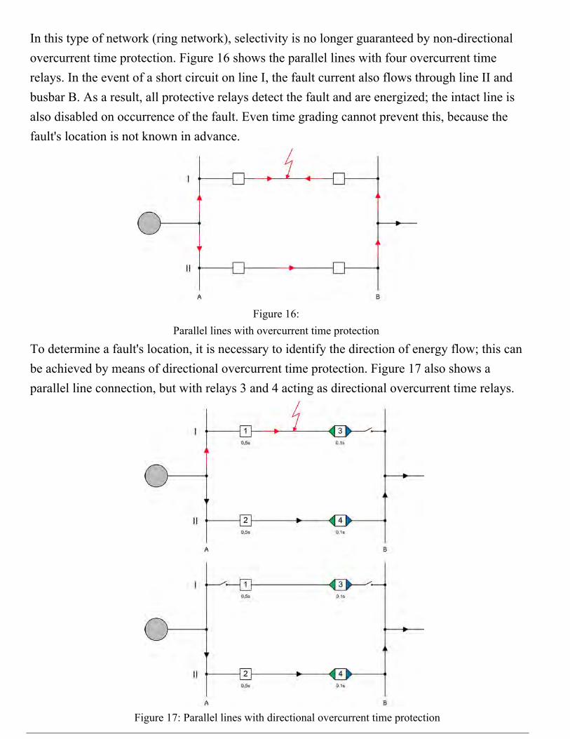
Figure 16:Parallel lines with overcurrent time protection

To determine a fault's location, it is necessary to identify the direction of energy flow; this can be achieved by means of directional overcurrent time protection. Figure 17 also shows a parallel line connection, but with relays 3 and 4 acting as directional overcurrent time relays.

Figure 17: Parallel lines with directional overcurrent time protection

In this type of network (ring network), selectivity is no longer guaranteed by non-directional overcurrent time protection. Figure 16 shows the parallel lines with four overcurrent time relays. In the event of a short circuit on line I, the fault current also flows through line II and busbar B. As a result, all protective relays detect the fault and are energized; the intact line is also disabled on occurrence of the fault. Even time grading cannot prevent this, because the fault's location is not known in advance.

On occurrence of a fault (e.g. on line I), all four protective relays respond again. The two non-directional overcurrent time relays 1 and 2 only detect an overcurrent. Of the two directional overcurrent time relays 3 and 4, relay 3 measures the fault current flowing in the reverse direction (green arrow) and trips after a short time span (Figure 17, left). Relay 4 measures the fault current flowing in the forward direction (blue arrow). This relay either remains inactive or serves as backup protection for line I and trips after a delay time if relay 3 has failed to trip.

Once relay 3 has tripped, no short-circuit current flows any longer through line II or busbar B, so that relay 2 is de-energized. In contrast to the directional overcurrent time devices, relays 1 and 2 are time-graded to provide time for direction recognition.

After a certain time delay, the already energized relay 1 trips. Line I is completely disconnected from the power grid, and intact line II remains serviceable but must now conduct the entire operating current (Figure 17, right). The excitation current chosen for the relays must prevent them from being energized once again in such situations.

INmax = INI + INIIII

INmax = Maximum operating current

INII == Operating current in line I

INIII = Operating current in line IIII

However, the maximum pick-up value must be low enough to make sure sufficient protection at the minimum fault current (at the end of the line).IKmin > IIANN==1.2*INmax > INmax

A Good guideline here is 1.2 times the maximum operating current. As made evident by the equation above, this value is higher than the maximum operating current and lower than the minimum fault current.

To set up direction recognition, protective relays can be individually set in terms of delay times for a variety of fault situations such as short circuit and overload, for enhancing selectivity, or for backup protection. Direction recognition additionally permits fault localization. This guarantee high selectivity and, therefore, reliable supply (n - 1 criterion).

First is defined the direction (forward or reverse) in which the relay will trip to provide primary protection. After the directions have been defined, the relays' time sequence must be set. Action is needed as soon as the direction of energy flow has been recognized following occurrence of a fault. The relays should only respond to energy flow in the set direction. To avoid false tripping, a delay time is set for the two non-directional relays. For a better understanding of the chronological sequences involved here, the tripping times are to be extended.

7.High Speed Distance Protection

Distance protection is a technique which, due to its higher selectivity, is applied particularly in meshed networks operating at high and extra-high voltages. As in the case of other protective techniques, distance protection devices must be energized in order to come into action. Typical excitation criteria here are overcurrent, undervoltage, earthing and underimpedance. It is important for the excitation value to lie above the maximum overload current so that the protective device does not respond to non-critical overloads. A good guideline for the pick-up value is 1.2 times the load current.

Distance protection is based on determination of impedance from current and voltage; the distance to the line fault as well as direction of energy flow can be discovered in this process. The measurement variables are coupled out via current and voltage transformers (Figure 18).

Figure 18:Current and voltage transformers

If the set pickup value is exceeded, the device determines the impedance (Figure 19) and then acts as required. The impedance is proportional to the distance between the fault and the protective device, thereby permitting this distance to be calculated. Directly at the fault's location, the voltage drops as far as 0 V and a short-circuit current IK flows. The current depends on the line's length. The calculated impedance is proportional to the length of the line if it exhibits a high degree of similarity. Figure 19 shows how the voltage increases with the distance to the fault.

Figure 19:Voltage dip at the fault's location

Depending on the length of the line, several distance protection devices are usually distributed along the line, hence dividing it into sections. The protective devices are normally combined with substations or switchgear stations such as those shown in Figure 19 (A, B, etc.). Each protective device acts as a primary protector for a dedicated line segment, general (backup) protection also being possible. This series-connection results in staggered (stepped) characteristics such as those indicated in Figure 20. The advantage of this staggering are the short tripping times in each section and the back-up protection available in case a device in a different section fails.

Figure 20:Single stepped characteristic

Figure 20 shows a typical stepped characteristic of a distance protection facility. The impedance values are assigned zones (Z) and tripping times (t). The zones are directional; it is also possible to set non-directional backup times to ultimately retain a capability to recognize faults in both directions.

Figure 21:

Swaggered stepped characteristics

Measuring the current and voltage additionally makes it possible to determine the direction of energy flow (directional zones). Energy flow's forward direction is defined as entering the protected line, reverse as leaving it. In Figure 21, this has the following implication::

Protective device B detects a forward flow of energy in the line section leading to device C, and a reverse flow of energy in the line section leading to device A.

The direction is chosen on the basis of the phase angle between the current and voltage. Figure 22 explain this principle. It shows that a current lag/lead of -22°< phi < +120° with respect to the voltage serves to define the forward direction, all other angles serving to define the reverse direction.

The first stage should be fast-acting (approximately 100 ms - inherent component time) and cover about 85% of the line's length. This prevents fast disconnection of faults right behind the next protective relay. Faults occurring over the remaining 15% of the line are shut off by the next stage (after about 400 ms). The remaining stages function accordingly (Figure 21).

Figure 22:Determining the phase angle

The distance protection devices can be set to provide a variety of trip characteristics, including circular and polygonal. In the case of the circular characteristic (Figure 23), an appropriate zone is selected in dependence on the impedance's value, and the tripping time assigned to this zone in the device is then applied. The phase angle determines the direction of energy flow.

Figure 23:Circular trip characteristic

The fault resistance (R) and fault reactance (X) are compared in the case of the polygon characteristic. The calculated values are compared with the reference levels, and the appropriate zone selected. Figure 24 shows the structure of this characteristic.

Figure 24:Polygonal trip characteristic

The polygonal characteristic is used to separately set the zone ranges in the R- or X-direction, for example, to better account for the influence of an arc fault or contact resistance in the event of a short circuit. Moreover, the polygons can be tilted to adapt to the line path. It is common practice to match the line path's and polygon's angles. The special advantages of distance protection are the short trip times and the absence of the control and communication cables which would otherwise be required for signal comparison. Direction identification additionally permits deployment in the case of double-ended feed and ring networks.

Bellow is a graphic example with steps and calculation to set up a distance protection relay:

First, we will determine the impedance zones with the help of the line impedances. For this purpose, let us take a look at Figure 25. In this model, the segment between stations A and B, for instance, involves a combination of two lines each 300 km (186,4 miles) long. To calculate impedance zones, imagine a further line segment (B - C) 600 km (372,8 miles) long enabling a definition of zones beyond the line to be protected by relay A. The reactance of the respective line segment is decisive for the range of each distance zone. As already familiar from the theoretical section, the first zone with impedance ZAB on line segment A - B is set to 85% of the distance and a delay time T1 of 0.00 seconds. The fault is thus isolated within the components' inherent time.

The other stages are determined according to the specifications in Figure 25. Zones 1 and 2 should each respond in the forward direction. Zone 3 should serve as non-directional, backup protection.

Figure 25: Network plan

With the help of the line impedances and Figure 25, zones 1 to 3 can be determined. Figure 26 shows the matching stepped characteristic.

Note: The indicated values correspond to the transformers' primary sides.

R /Ω R' /' L /mH

300 Km 7,2 0,024 230 86.7

600 Km 14,4 0,024 460 173.41

Calculation of the impedances ZAB and ZBC (600 Km line) ZAB = ZBC = (R + jX) = (14,4Ω + j173.41) Zone settings for selective steppingPrimary Values

Formula Results

Zone 1 0,85*ZAB (12.24 Ω + j147.39 Ω)

Zone 2 0,85*(ZAB + 0,85*ZBC ) (22.64 Ω + j272.68 Ω)

Zone 3 (ZAB ++ZBC) (28.8 Ω + j 346.82 Ω)

X=ω*L/Ω

Figure 26: Grading scheme

Secondary ValuesDuring set up of the protective device, some of the values need to be specified for the secondary side of voltage and current transformers and must therefore be converted beforehand. When calculating voltages and currents, this conversion is performed via the transformation ratios. For impedance calculation:

Formula

Zone 1 Transformation ratio * ZZone 1 (Primary)



Characteristic DataTrippingtime

Z1 - t1 Z2 - t2 Z3 - t3

0.00 s 5.00 s 10.00 s

Phase angle = for Im{Z} > 0 and any Re{Z}

With the help of the impedance zones determined for the secondary side, the full polygonal characteristic can be constructed. For this purpose you draw the line path first and then align the polygon with it. As seen it in Figure 27:

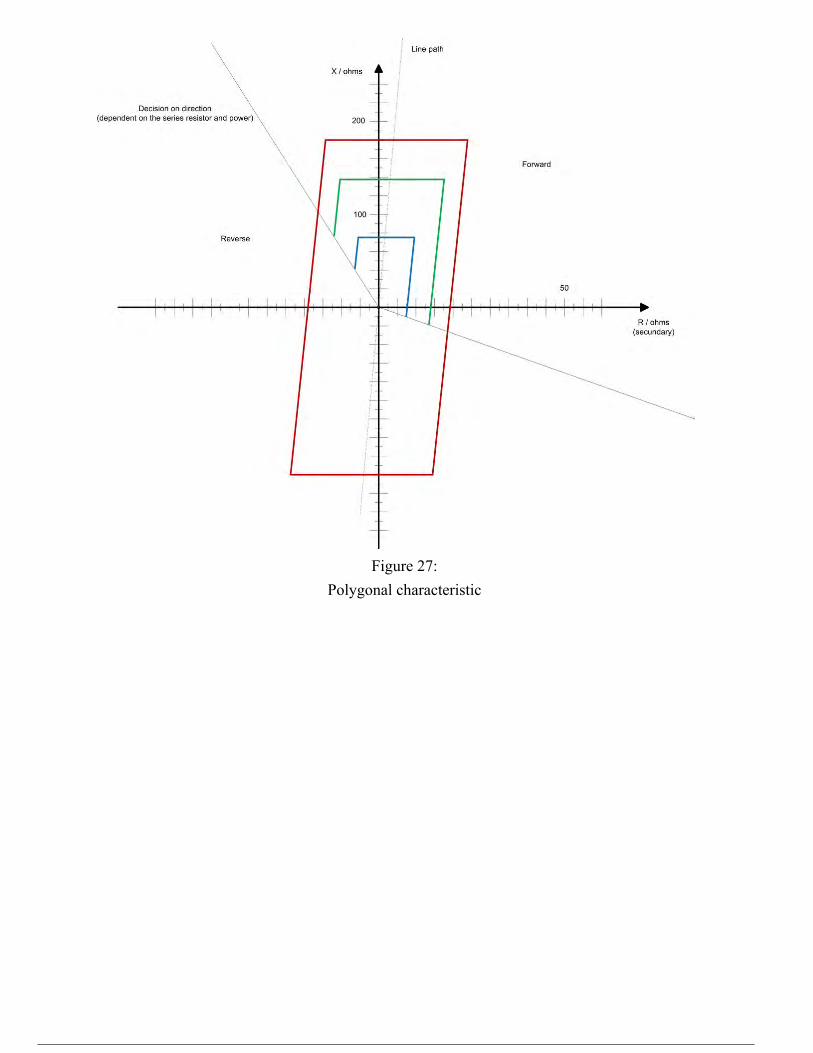
Figure 27:Polygonal characteristic

Objectives

Introduction to protection technology with theoretical and practical investigation of overcurrent time protection using the related software provided (SCADA). The resources necessary to protect lines and associated fault types are introduced and explained. Determination of reset ratios (hysteresis) to analyze the operating principles and accuracy of digital protective relays. Setting options and overcurrent time protection characteristics are demonstrated in a subsequent test of trip response.

1. Theoretical principles of protection technology and overcurrent time protection.2. Establish reset ratio in the case of single, two and three pole short circuit.3. Testing a circuit breaker's trip characteristic in the event of a fault.

Overcurrent Time Protection

Assembly Instructions

Make sure that the transmission line model is not covered with the template to 150 km (93,2 miles) through the sensors unless explicitly specified.

The overhead transmission line receives a three-phase power supply and is loaded symmetrically at its end. Located before the transmission line is a circuit breaker (power-switch module) to disconnect the line from the power supply in the event of a fault. The time overcurrent relay measures the current in each phase via a current transformer.

Set up the experiment as shown in the circuit diagram (Figure 28) and layout plan (Figure 29) below.

1. 3-phase power supply2. Power-switch module3. Current transformer4. Transmission Line model5. Load6. Time overcurrent relay

Figure 28: Circuit diagram

Figure 29:Layout plan

Configuration of the SCADA interface:

1. Save the linked file: ELP1.pvc2. Open the "Lucas-Nülle SCADA Viewer" and select/open the file you saved in step 1.3. Click or go to "Diagnostics" → "Device Manager..." and configure all the equipment

in SCADA as specified in the section "Configuring SCADA for PowerLab".

Procedure

1. Determining Reset Ratios

During these experiments, you will need to increase the voltage gradually. Perform such increases slowly while observing the resultant reading on the ammeter. The potentiometers should be adjusted precisely and the switching times should be

measured. Use the supplied SCADA file interface ELP1.pvc. Instructions for the necessary

operating elements can be found in section "Configuring SCADA for PowerLab →Connection via RS485 → Configuration of protective equipment".

Set the resistive load CO3301-3F to 750 Ω. Set the relay's DIP switches as indicated in the table below. (active setting = yellow

background)

Function Trip Trip Trip Block I>

Block I>> f t I> t I>

DIP switch 1 2 3 4 5 6 7 8

ON Inverse Strong i.

Extreme i. Yes Yes 60 Hz x 10 s x 100 s

OFF DEFT DEFT DEFT No No 50 Hz x 1 s x 1 s

RivasHV

Highlight

RivasHV

Highlight

RivasHV

Highlight

RivasHV

Highlight

RivasHV

Highlight

RivasHV

Highlight

RivasHV

Highlight

RivasHV

Highlight

Case 1: Symmetric, Three-pole Short Circuit

1. Connect the power-switch module 2 as shown in Figure 30 so that the right-hand side isbridged, and the left-hand side connected to all three phases at the overhead line's end.

2. On relay CO3301-4J (XI1-I), set the overcurrent level I> to 0.5 A and all otherpotentiometers to 0. See Figure 31.

3. Make sure that the source voltage is 0 V.4. Turn on both power switches modules.5. Turn on the three- phase power supply and slowly increase the voltage until the relay is

energized (red upper LED comes on).6. Read the current on the three-phase meter and record the pickup value IPU in the Table 1.7. Slowly reduce the voltage on the three-phase power supply until the relay is de-energized

again (red upper LED goes off).8. Read the current on the three-phase meter and record the release value IRe in the Table 1

below.9. Calculate the reset ratio R from the pickup value IPU and release value IRe (R = IRe / IPU).

Record this value in Table 1.10.Open power switches modules 1 and 2 (OFF buttons), turn the source voltage back to 0

V, and power off the three-phase power supply.11.Repeat this procedure at overcurrent (I>) levels 0.8 A, 1.0 A and 1.2 A, following Steps

2-10 above.

Table 1: Three-pole short circuit

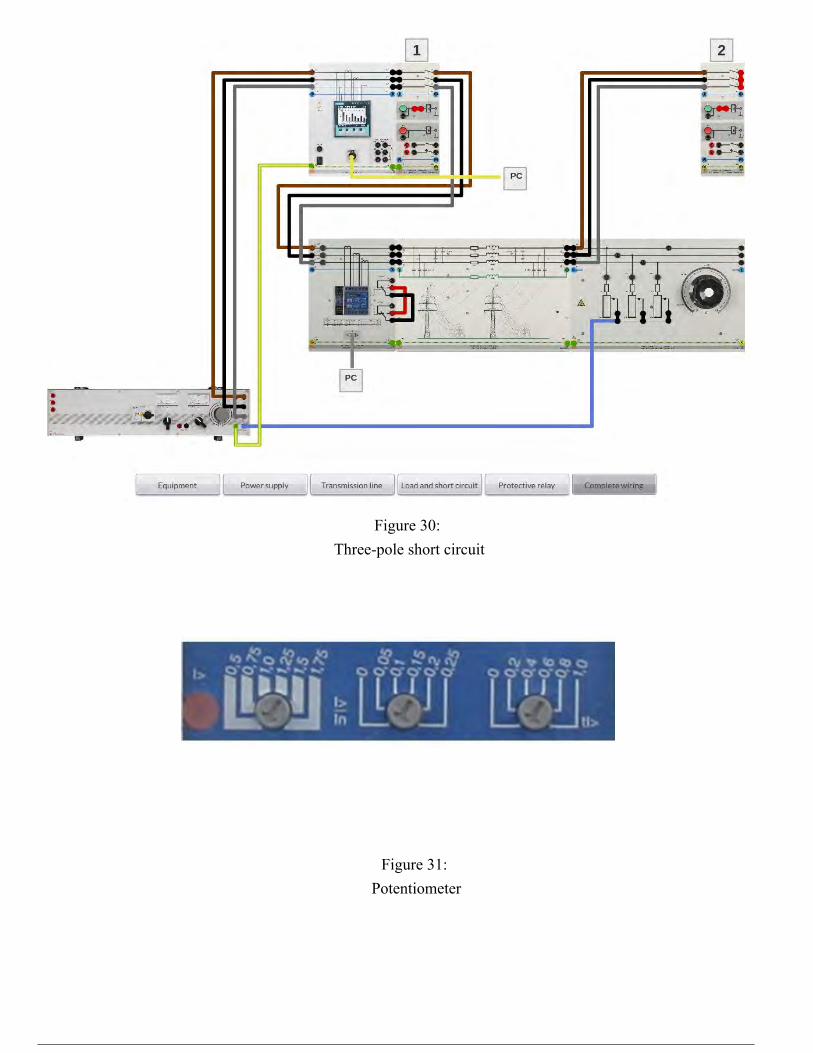
Figure 30: Three-pole short circuit

Figure 31: Potentiometer

Case 2: Two-pole Short Circuit

1. Connect the power-switch module 2 as show Figure 32 so that the right-hand side isbridged, and the left-hand side connected to two phases at the overhead line's end.








2-10 above.

Table 2: Two-pole short circuit

Figure 32:Two-pole short circuit


Case 3: Single-pole Short Circuit

1. Connect the power-switch module 2 as show Figure 34 so that the right-hand side isbridged, and the left-hand side connected to one phases and the N-Conductor.








2-10 above.

Table 3: Single-pole short circuit

Figure 34: Single-pole short circuit


2. Testing Trip Levels

Set up the experiment as shown in Figure 36. Establish the connection between theOFF button and the 24 VDC power supply of power switch module 1 as well asrelay outputs 24/21 and 14/11.

For relay CO3301-4J (XI1-I), configure the current overload trip threshold I> to 0.5A, I>/In to 0 and tl> to 0.5. As seen in Figure 37.

Use the supplied SCADA file interface ELP1.pvc. Instructions for the necessaryoperating elements can be found in section "Configuring SCADA for PowerLab→ Connection via RS485 → Configuration of protective equipment".

Set the relay's DIP switches as indicated in the table below. (active setting = yellowbackground)

Function Trip Trip Trip Block I>

Block I>> f t I> t I>

DIP switch 1 2 3 4 5 6 7 8

ON Inverse Strong i.

Extreme i. Yes Yes 60 Hz x 10 s x 100 s

OFF DEFT DEFT DEFT No No 50 Hz x 1 s x 1 s


RivasHV

Highlight

RivasHV

Highlight

RivasHV

Highlight

RivasHV

Highlight

RivasHV

Highlight

RivasHV

Highlight

RivasHV

Highlight

RivasHV

Highlight

Figure 36:Layout plan

Case 1: Test of the Short Circuit Level

1. Make sure that power switch module 2 is open (OFF button).2. Check the potentiometer settings once again.3. Turn the resistive load CO3301-3F control up to 500 Ω, so that the white arrow points at

the according mark.4. Power on the three-phase power supply and set the line-to-line voltage VL-L = 220 V.5. Turn on power switch module 1 (ON button).

The configuration is now in its normal operating mode.6. Check the connections for power switch 2. Three phases at the end of the line must be

linked together.7. Produce a three-pole short circuit by closing power switch 2 (ON button).8. Mark in Table 4 the correct active stage and trip delay time occurring due to previous

Step 7.9. Open power switch modules 1 and 2 (OFF Buttons), turn the source voltage back to 0 V,

and power off the three-phase power supply.

Table 4: Short-Circuit Level

Case 2: Test of the Overload Level

1. Make sure that power switch module 2 is open (OFF button).2. Check the potentiometer settings once again.3. Turn the resistive load CO3301-3F control up to 500 Ω, so that the white arrow points at

the according mark. (Load Setting Unchanged).4. Power on the three-phase power supply and set the line-to-line voltage VL-L = 220 V.5. Turn on power switch module 1 (ON button).

The configuration is back in its normal operating mode.

6. We will now simulate an overload. For this purpose, decrease the load resistanceslowly until the relay responds.

7. Mark in Table 5 the correct active stage and trip delay time occurring due to previous

Step 6.8. Open power switch modules 1 and 2 (OFF Buttons), turn the source voltage back to 0 V,

and power off the three-phase power supply.

Table 5:Overload Level

Report Questions1. Where is the overcurrent time protection normally used and what are its disadvantages?2. Name the fast tripping stage in overcurrent time protection.3. What is the average reset ratio R (Hysteresis) among the three cases of determinig the reset

ratio in overcurrent time protection? Why does it deviate from 1?4. Plot IPU and IRE vs I> for Tables 1 - 3.5. Name the two magnitudes of relevance in directional overcurrent protection and how it

calculates energy's flow direction.6. What are the trip characteristic of directional overcurrent protection?.7. Which equipments use overvoltage protection relays and which ones use undervoltage

protection relays?8. Where is the directional power protection mainly used?.9. What is the fast response range of directional power protection and why its release time so

long?10.During parallel operation of two power generators, what happens if one of the generator

turbines fails?11.Which grids apply earth fault monitoring?12.Name the magnitude measurement criteria used during earth fault protection and how much

is its value.13.Specify the correct sequence of earth faults in the grid due to the grid's capacitances and

inductances.14.What is the n-1 principle?15.How the directional overcurrent time relays increase selectivity in protection of parallel

transmission lines?16.How must be defined the configuration of directional overcurrent time relays in protection

of parallel transmission lines, in terms of excitation and maximum operating current?

ReferencesNils Gilleßen, Protective Systems for High-voltage Transmission Lines, Lucas-Nülle GmbH, 2019.

protection technolo protective systems for high-voltage

Documents