EUROPEAN ORGANIZATION FOR NUCLEAR RESEARCH

CERN-SPSC/99-35SPSC/P315

15 November, 1999

Proposalto study hadron production

for the neutrino factory and forthe atmospheric neutrino flux

ii

M.G. Catanesi, M.T. Muciaccia, E. Radicioni, P. Righini, S. SimoneUniversita degli Studi e Sezione INFN, Bari, Italy

I. Boyko, S. Bunyatov, G. Chelkov, D. Dedovitch, P. Evtoukovitch, L. Gongadze, G. Glonti,M. Gostkin, S. Kotov, D. Kharchenko, O. Klimov, Z. Kroumchtein, Y. Nefedov, M. Nikolenko,

B. Popov, I. Potrap, A. Rudenko, E. Tskhadadze, V. Serdiouk, V. Zhuravlov.Joint Institute for Nuclear Research, JINR Dubna, Russian Federation

M. Doucet, F. Dydak∗, J-P. Fabre, A. Grant, L. Linssen, J. Panman, I.M. Papadopoulos,F.J.P. Soler, P. Zucchelli

CERN, Geneva, Switzerland

R. EdgecockRutherford Appleton Laboratory, Chilton, Didcot, UK

A. Blondel1

Section de Physique, Universite de Geneve, Switzerland

U. GastaldiLaboratori Nazionali di Legnaro dell’INFN, Legnaro, Italy

G. GregoireUCL, Louvain-la-Neuve, Belgium

M. Bonesini, M. Calvi, S. Gilardoni, M. Paganoni, A. PulliaUniversita degli Studi e Sezione INFN, Milano, Italy

S. Gninenko, M. Kirsanov, Yu. Musienko, A. Poljarush, A. ToropinInstitute for Nuclear Research, Moscow, Russia

V. PalladinoUniversita “Federico II” e Sezione INFN, Napoli, Italy

M. Baldo Ceolin, F. Bobisut, D. Gibin, A. Guglielmi, M. Laveder, M. MezzettoUniversita degli Studi e Sezione INFN, Padova, Italy

J. Dumarchez, F. VannucciUniversite de Paris VI et VII, Paris, France

U. DoreUniversita “La Sapienza” e Sezione INFN, Roma, Italy

M. Chizhov, D. Kolev, R. TsenovFaculty of Physics, St. Kliment Ohridski University, Sofia, Bulgaria

G. Giannini, G. SantinUniversita di Trieste e Sezione INFN, Trieste, Italy

A. Cervera-Villanueva, J. Diaz, A. Faus-Golfe, J.J. Gomez-Cadenas, M.C. Gonzalez-Garcia,J. Velasco

University of Valencia, Valencia, Spain

P. GruberInstitut fur Kernphysik, Technische Universitat, Wien, Austria

∗contact-person1now at Ecole Polytechnique, Palaiseau, France

iii

iv

Contents

1 Introduction and summary 1

2 Physics motivation and goals 2

2.1 Neutrino factory . . . . . . . . . . . . . . . . . . . . . . . . . . . . . . . . . . . . 2

2.1.1 Pion production in a neutrino factory . . . . . . . . . . . . . . . . . . . . 2

2.1.2 Parameters . . . . . . . . . . . . . . . . . . . . . . . . . . . . . . . . . . . 3

2.1.3 Desired experimental data . . . . . . . . . . . . . . . . . . . . . . . . . . . 4

2.2 Atmospheric neutrino flux . . . . . . . . . . . . . . . . . . . . . . . . . . . . . . . 5

2.3 Scope of the experiment . . . . . . . . . . . . . . . . . . . . . . . . . . . . . . . . 7

2.3.1 What is required? . . . . . . . . . . . . . . . . . . . . . . . . . . . . . . . 7

2.3.2 What is experimentally possible? . . . . . . . . . . . . . . . . . . . . . . . 8

2.3.3 Precision requirements . . . . . . . . . . . . . . . . . . . . . . . . . . . . . 8

2.4 Particle identification . . . . . . . . . . . . . . . . . . . . . . . . . . . . . . . . . . 8

3 Experimental setup 11

3.1 Beam and experimental area . . . . . . . . . . . . . . . . . . . . . . . . . . . . . 11

3.2 Overview of the spectrometer . . . . . . . . . . . . . . . . . . . . . . . . . . . . . 13

3.3 Targets . . . . . . . . . . . . . . . . . . . . . . . . . . . . . . . . . . . . . . . . . 15

3.4 Time projection chamber . . . . . . . . . . . . . . . . . . . . . . . . . . . . . . . 16

3.4.1 The ALEPH TPC90 . . . . . . . . . . . . . . . . . . . . . . . . . . . . . . 16

3.4.2 The solenoidal magnet . . . . . . . . . . . . . . . . . . . . . . . . . . . . . 17

3.4.3 The TPC mechanics . . . . . . . . . . . . . . . . . . . . . . . . . . . . . . 18

3.4.4 TPC performance . . . . . . . . . . . . . . . . . . . . . . . . . . . . . . . 18

3.4.5 The TPC electronics . . . . . . . . . . . . . . . . . . . . . . . . . . . . . . 19

3.5 Spectrometer magnet . . . . . . . . . . . . . . . . . . . . . . . . . . . . . . . . . . 19

3.6 NOMAD drift chambers . . . . . . . . . . . . . . . . . . . . . . . . . . . . . . . . 20

3.7 Gas Cherenkov detector . . . . . . . . . . . . . . . . . . . . . . . . . . . . . . . . 21

3.8 Time-of-flight wall . . . . . . . . . . . . . . . . . . . . . . . . . . . . . . . . . . . 23

3.9 Muon identifier . . . . . . . . . . . . . . . . . . . . . . . . . . . . . . . . . . . . . 24

4 Trigger 25

v

4.1 Running conditions . . . . . . . . . . . . . . . . . . . . . . . . . . . . . . . . . . . 26

4.2 Trigger layout . . . . . . . . . . . . . . . . . . . . . . . . . . . . . . . . . . . . . . 27

4.3 Trigger conditions . . . . . . . . . . . . . . . . . . . . . . . . . . . . . . . . . . . 28

5 Data acquisition and computing 29

5.1 Introduction . . . . . . . . . . . . . . . . . . . . . . . . . . . . . . . . . . . . . . . 29

5.2 Readout and data volumes . . . . . . . . . . . . . . . . . . . . . . . . . . . . . . . 29

5.3 Network topology . . . . . . . . . . . . . . . . . . . . . . . . . . . . . . . . . . . . 31

6 Performance of the spectrometer 31

6.1 Momentum measurement . . . . . . . . . . . . . . . . . . . . . . . . . . . . . . . 33

6.2 Particle Identification . . . . . . . . . . . . . . . . . . . . . . . . . . . . . . . . . 33

6.3 Results of the simulation . . . . . . . . . . . . . . . . . . . . . . . . . . . . . . . . 34

6.3.1 Geometrical acceptance . . . . . . . . . . . . . . . . . . . . . . . . . . . . 34

6.3.2 Particle identification efficiency . . . . . . . . . . . . . . . . . . . . . . . . 35

6.3.3 Combined Acceptance and efficiency . . . . . . . . . . . . . . . . . . . . . 36

7 Cost estimate 37

8 Schedule 38

vi

1 Introduction and summary

It is proposed to carry out at the CERN PS a programme of measurements of secondary hadrons,over the full solid angle, produced on thin and thick nuclear targets by beams of protons andpions with momentum in the range 2 to 15 GeV/c.

The main motivation is twofold: to acquire adequate knowledge of pion yields for an optimaldesign of the recently proposed intense neutrino source based on muon decay in a muon storagering (neutrino factory); and to improve substantially the calculation of the atmospheric neutrinoflux which is needed for a refined interpretation of the evidence for neutrino oscillation from thestudy of atmospheric neutrinos in present and forthcoming experiments.

Additional motivations are: a measurement of the yield of low-momentum backward-going pionswhich could be used for a high-intensity stopped-muon source as a by-product of the neutrinofactory; and a better precision of the fluxes in conventional neutrino beams such as at theKEK 12 GeV/c proton-synchrotron, important for the K2K experiment, and at the low-energy(8 GeV/c) booster at Fermilab, used for the MiniBooNe experiment.

A neutrino factory requires a sophisticated front-end: the proton target, pion capture, pionphase rotation, pion decay, muon capture, and muon cooling. Existing data on the overall yieldand distribution in phase space of pions produced in low-energy proton–nucleus collisions arenot adequate for a quantitative and optimized design. For the proton source, several optionsas diverse as a 2 GeV/c proton linac and a 16 GeV/c rapid-cycling synchrotron are underdiscussion. Deuterons, which provide more symmetric yields of positive and negative pions thanprotons, are discussed as an alternative to protons. As in the case of a 2 GeV/c proton linac thelargest pion yield is expected for pions with momentum ∼ 200 MeV/c, the proposed experimentaims at the identification and measurement of pions down to momenta well below 100 MeV/c.

The existing ∼ 30% uncertainty in the calculation of absolute atmospheric neutrino fluxes andthe ∼ 7% uncertainty in the ratio of neutrino flavours could be substantially reduced by measur-ing the spectrum of positive and negative pions produced by protons in the full range of PS beammomenta. This is relevant for the interpretation of current results from SuperKamiokande [1, 2]and even more so for future atmospheric neutrino experiments which are expected to make useof atmospheric neutrinos down to an energy of 100 MeV. Also, pion production by helium nu-clei is important, as helium nuclei constitute ∼ 10% of the primary charged-particle cosmic-rayflux. Existing data are mostly from single-arm hadron production experiments [3, 4] which werecarried out in the seventies. Present models and computer generators of hadron production inproton–nucleus collisions in the atmosphere have been tuned to describe these data. However,the scale error in these experiments was estimated at 15% or more, mostly arising from accep-tance uncertainties. In addition, at low momenta where different models for pion production onnuclei make very different predictions of atmospheric neutrino fluxes, experiments either did notprovide any data at all or lacked particle identification capable of separating pions from protons.

The E910 experiment at BNL [5] took data in 1996 which will be relevant to some of the issuesmentioned above. The experiment’s goal was the study of strange matter production by protonson nuclei, with a view to making a comparison with nucleus–nucleus collisions. First papers on‘centrality’ measurements were published recently [6]. There is overlap between E910 and theproposed experiment at high proton momenta, as E910 took data at proton momenta of 6, 12and 18 GeV/c. The 6 GeV/c data have low statistics. No data were taken with thick targets.

The proposed experiment comprises a large-acceptance charged-particle magnetic spectrometerof conventional design, located in the East Hall of the CERN PS and using the T9 tagged

1

charged-particle beam. It will re-use existing equipment as much as possible, notably fromthe NOMAD [7] and CHORUS [8] experiments. Of particular importance is the re-use of theALEPH prototype TPC [9], albeit with substantial modifications. The only major piece to benewly built is a threshold Cherenkov detector with gas at atmospheric pressure.

It is planned to have a technical run in the end of 2000, and the physics run in 2001. For theyear 2002, a second phase of the experiment is under discussion [10] with a view to removingthe primary proton target and sending deuterium and helium nuclei directly to the target of theexperiment.

Although the dominant uncertainties in the atmospheric neutrino fluxes will be removed by theproposed experiment, an extension to higher beammomenta in a third phase, up to∼ 100 GeV/c,could be contemplated, including running with helium ions. Such a program would not onlyextend reliable calculations of atmospheric neutrino fluxes into the 100 GeV/c region, but alsocontribute to solving the puzzle of the ‘knee’ of the charged-particle cosmic-ray spectrum around3 × 1015 eV. Progress in this area is hampered no longer by the lack of availability of gooddata, but by their interpretation in terms of atmospheric shower models. Such models not onlyneed better experimental input on the interaction of the very high-energy primaries, but also onthe interactions of lower-energy secondaries with oxygen and nitrogen. It is with respect to thelatter aspect that this experiment can provide useful input.

Certain measurements with higher beammomenta are within reach of the COMPASS experimentat the SPS.

2 Physics motivation and goals

2.1 Neutrino factory

A neutrino factory is a complex machine to produce neutrinos from circulating muons decayingin a storage ring [11]. Controlling the muon-beam characteristics will allow a well collimatedν beam of high intensity and high energy to be obtained. The aim is to achieve intensities of1020 to 1022 µ per year in the decay ring. The highest conventional neutrino flux is currentlyplanned for the MINOS near detector with 1018 νµ and 5 × 1015 νe per year [12].

The generic layout of a neutrino factory (see Fig. 1) consists of a proton accelerator, a target anda muon storage ring [13]. A high power (4 MW) proton beam impinges on a target producingpions which are collected with a high magnetic field. In a drift space, they decay into a muonand a muon neutrino that is lost (π+ → µ+ + νµ). After this, the muon phase space is reducedwith ionization cooling, the muons are accelerated to energies of up to 50 GeV and fed into adecay ring where they decay into an electron/positron and two neutrinos (µ+ → e+ + νe + νµ).The muons decaying in the straight sections of this ring produce a high intensity neutrino beamthat points towards a neutrino detector, allowing neutrino oscillation experiments with highprecision. By changing the sign of the charge of the collected pions it is possible to get the twoconjugated neutrinos, νe + νµ.

2.1.1 Pion production in a neutrino factory

In this context, accurate pion production yields are very important to achieve the desired neu-trino fluxes and to design a cost-effective machine [14]. The design goal is to maximize the figure

2

Figure 1: Generic Layout of a Neutrino Factory.

of merit, which is the number of accelerated muons in the decay ring of each sign. The time formeasuring a certain number of events in an oscillation experiment should be minimized, thusthe goal is to maximize both pion production rates. With the pion production rate per protonper unit of energy rπ = nπ/(np ·GeV) we get the expression to be minimized:

1rπ+

+1

rπ−. (1)

Current simulations of the pion yield with FLUKA and MARS show a 30%–100% discrepancyin the pion production [15]. It is reasonable to assume a similar uncertainty for the momentumdistribution. The reason for this uncertainty is the small amount of underlying experimentaldata for the simulation programs. A high-precision pion production experiment would thus bea requirement for the simulation of a neutrino factory.

2.1.2 Parameters

The variables affecting the pion production are proton energy, target material and target geom-etry (diameter and length). The total proton-beam power is only a scaling parameter. A pionproduction experiment should give the set of data necessary to optimize both proton energyand target material in order to achieve the highest number of potentially collected pions of bothcharge signs per unit of energy.

3

Table 1: Proposed proton drivers [13].CERN CERN FNAL JHF

BNLLinac + Synch. Synch. Synch.

AccumulatorProton momentum GeV/c 2 24 16 50Repetition Rate Hz 50 5 15 2.5Proton beam Power MW 4 4 4 4Number of protons per pulse 1014 1.3–2.6 2 1 2

Table 2: Desired parameters of the experiment.Parameter RangeProton momentum 2–24 GeV/c; 1–2 GeV/c stepsAngular acceptance 4πTarget thickness thin, 1 and 2 interaction lengthsTarget materials Li, Be, C, Al, Ni, Cu, liq. Ga-Sn, W, liq. Hg

A list of proton drivers under consideration in different laboratories is given in Table 1. Theyare all based on upgrades of existing machines, except the CERN scenario of a 2 GeV/c linacthat could be based on super-conducting LEP cavities.

Several target materials have been proposed, starting from low-Z materials such as Be and Liover C to high-Z materials such as Ni, Cu, liquid Hg, or W. In addition, deuterium has beenproposed as target material for a recirculating proton scheme [16]. Apart from efficient pionproduction, cooling the target is a major concern in choosing the right material. Estimatesshow that, depending on the proton energy, up to 30% of the proton power is dissipated in thetarget and has to be cooled. Even though the proposed experiment is a low-intensity one, hintson the energy deposition in the target can give valuable information to design the target-coolingsubsystem. A list of the desired experimental parameters is shown in Table 2.

2.1.3 Desired experimental data

The data taken in the experiment will be used to validate the design of the neutrino factorydownstream the target. The transverse capture and the first phase rotation are strongly depen-dent on the pion production data. The transverse momentum distribution of the pions mustbe known to a high precision as it affects the efficiency of transverse capture. At first sight thelongitudinal momenta are not required to be known with such an accuracy, as a wide range ofthem will be captured. Although this argument is valid for capture, this is not the case forthe first phase rotation where the pion beam is nearly mono-energetic (in order to distinguishbetween forward- and backward-decaying pions for enhanced polarization of the muon beam).A high precision on the longitudinal momentum is therefore also necessary.

The overall pion yield per incident proton will be a scaling parameter for the figure of merit ofthe neutrino factory. A precision of 5% in the pion yield will be sufficient. The same accuracyis required for the ratio of π+ to π−, as the particle with lower production yield determinesthe proton-beam power needed. The desired data to be taken in the experiment are shown in

4

Table 3: Desired data.Parameter Range Precisionπ longitudinal momentum 100–700 MeV/c < 25 MeV/cπ transverse momentum 0–250 MeV/c < 25 MeV/cNumber of secondary π/proton 5%π+/π− ratio 5%

Table 3.

2.2 Atmospheric neutrino flux

The SuperKamiokande collaboration has presented evidence for neutrino oscillation based on ahigh-statistics sample of atmospheric neutrino interactions [1, 2]. The detailed interpretation ofthese data, as well as the comparison with measurements at different locations and with differenttechniques, requires reliable calculations of fluxes of atmospheric neutrinos.

Several one-dimensional calculations of the flux of atmospheric neutrinos have been published [17,18, 19, 20]. Recently, more sophisticated three-dimensional calculations have become avail-able [21, 22]. However, it has been claimed by Battistoni et al. [21] that for practical purposesthe one-dimensional calculations give adequate results. Therefore, it makes sense to includeboth one- and three-dimensional calculations in the comparison of the results of different calcu-lations. The various calculations quote large errors and differ significantly in their results. Thesedifferences have attracted quite some attention and have been extensively analyzed [23, 24, 25].The dominant sources of discrepancies were found in

• the assumed energy spectrum and the chemical composition of the primary cosmic rays;and

• the representation of pion production in collisions of the primaries with nitrogen andoxygen nuclei.

Next in the order of uncertainties is the neutrino-nucleon cross-section, which is surprisinglyuncertain at low energy. Ultimately, measurements in so-called ‘near’ detectors at the neutrinofactory will entirely eliminate this latter source of error.

There used to be sizeable (up to 30%) differences between measurements of the primary flux;however thanks to several new measurements [26, 27, 28] there is a tendency toward convergence,and hopes are that with a new round of long-duration balloon flights this uncertainty will bereduced and will become insignificant within a few years. This leaves the representation of pionproduction on light nuclei as the only remaining major obstacle to a precise (i.e. few per cent)calculation of the atmospheric neutrino flux in contrast to its current uncertainty of ∼ 30% forneutrino energies Eν < 10 GeV.

For lower-energy neutrino events such as the ‘sub-GeV’ sample of SuperKamiokande, the parentcosmic-ray primaries have energies in the range 5–100 GeV as shown in Fig. 2 taken fromRef. [29].

For the atmospheric neutrino flux, the overall yield of pions is all-important, integrated overthe full phase space. The value of measurements therefore depends on the overall normalization

5

Res

pons

e fo

r su

b-G

eV n

eutr

ino

inte

ract

ions

0 .5 1 1.5 2 2.50

.1

.2

.3

Figure 2: Response for ‘sub-GeV’ neutrino events in Su-perKamiokande to the en-ergy of cosmic-ray primaries.Curve A: no geomagneticcut-off; Curve B: events frombelow; Curve C: events fromabove. Each pair of curvesgives the range of solar activ-ity between minimum (solid)and maximum (dotted).

precision of the experiment, and on its phase-space coverage.

To illustrate the problem, Fig. 3 taken from Ref. [29] shows the fraction of the phase spacewhich falls inside the acceptance of various experiments measuring pion production by protonson beryllium [3, 4, 30]. The unmeasured regions have to be covered by extrapolation guided bymodels of pion production.

0

0.2

0.4

0.6

0.8

1

0 0.2 0.4 0.6 0.8 1

mea

sure

d fr

actio

n of

cro

ss s

ectio

n

xlab

Eichten et al., π+

Allaby et al., π+

Abbott et al., π+

Figure 3: Fraction of pionproduction cross-section cov-ered by different pion pro-duction experiments in p–Beinteractions.

To the uncertainty in this extrapolation other sources of uncertainty have to be added. Theoverall normalization error of the experiments was typically 15%. The lack of data on nitrogen-like nuclei makes necessary yet another extrapolation from beryllium data. Finally, it is to

6

be recalled that ∼ 15% of the primary cosmic-ray nucleons are bound in helium nuclei andmeasurements of production yields from their interactions with oxygen and nitrogen nuclei arenot available.

The conclusion from the above discussion is that a single high-precision large-acceptance pro-duction experiment is needed which measures pion production by protons and helium nuclei onnitrogen and oxygen targets. With these data in hand, in a few years time, the event rate fromatmospheric neutrinos will be calculable with a few per-cent precision.

2.3 Scope of the experiment

2.3.1 What is required?

The design considerations of the neutrino factory require the following measurements:

• Proton beam with momentum between 2 and 24 GeV/c.

• Thick high-Z targets. However, since the proton target of the neutrino factory is in avery high magnetic field, its final efficiency for pion production will be determined froma combination of thin- and thick-target measurements, and calculations. The calculatedthick-target yield in a non-magnetic environment is checked by measurement.

• Secondary pion yield over the phase space: 100 MeV/c < pL < 700MeV/c and pT <250MeV/c; secondary proton yield to assess problems of induced radiation.

• Deuterium beams with momentum of 1 GeV/c per nucleon to assess its usefulness for abetter π+ /π− ratio than obtained with a proton beam.

• Yield of backward-going pions to assess its usefulness for a high-intensity stopped-muonsource.

For a reliable calculation of the atmospheric neutrino flux down to 100 MeV energy, the followingmeasurements are needed:

• Proton and pion beam with momentum between 1 and 100 GeV/c.

• Targets of oxygen and nitrogen nuclei.

• Secondary π+, π−, K+, K− and proton yields over the full phase space, with particleenergy as the kinematical quantity of primary interest. The precision requirement is a fewper cent for π+, π− and proton, and ∼ 10% for kaons.

• Helium ions with momentum between 0.5 and 50 GeV/c per nucleon to complement theproton data.

In the context of atmospheric neutrinos, it should be recalled that the measurement precision ofthe π0/e ratio in SuperKamiokande, which is relevant for the question whether a sterile neutrinois required, depends on the precision of the measurement of the π0 production via neutralcurrents in the K2K experiment at KEK. This experiment is in turn limited by the knowledge ofpions and kaons produced by 12 GeV/c protons on a thick Al target. The results of the proposedexperiment would be instrumental in achieving a better precision on this important cross-section.

7

The MiniBooNe experiment at Fermilab would also benefit from precision measurements of8 GeV/c protons on a thick Al target. This experiment aims to refute or confirm the LSNDneutrino oscillation claim.

2.3.2 What is experimentally possible?

The two main constraints of the proposed experiment are the available beam momenta of theT9 beam line in the East Hall, which is limited to 15 GeV/c and the need to re-use existingequipment as much as possible, with a view to gaining time and minimizing capital expenditure.

Altogether, the following scenario emerges:

• Stage 1: T9 beam in the East Hall with proton and pion beams in the range 2–15 GeV/c;several thin targets spanning the full range between Be and W nuclei; a selection of thicktargets.

• Stage 2: T9 beam line in the East Hall, with the primary proton target removed, anddedicated PS running with deuterium and helium beams at selected momenta. Additionaltargets.

• Stage 3: An experiment at the SPS with a secondary beam momentum between 15 and100 GeV/c as well as with deuterium and helium beams at selected momenta. It is expectedthat COMPASS has the potential to perform some of these measurements.

At this point in time, approval is sought for Stage 1 only.

2.3.3 Precision requirements

Both for the neutrino factory and for the atmospheric neutrino flux, an overall precision of 2%for the inclusive cross-section of secondary particles is the primary aim. This is motivated by thewish to obtain 5% precision both on the production of accepted muons in the neutrino factory’sfront stage, and on the atmospheric neutrino flux. Either prediction will involve uncertaintiesbeyond those of the results of the proposed experiment.

A 2% overall accuracy requires some 104 events for each measured point, of which there aremany. It will take several months of running time to achieve sufficient statistical precision (seesection 4).

Acceptance calculations are potentially more precise with modern simulation tools than previ-ously, when typically a 10% precision was considered satisfactory. The largest challenge comesfrom understanding efficiencies with an error of order 1%. This calls for as much redundancyas can be afforded, with a view to cross-calibrating efficiencies. For example, pion/proton iden-tification is provided by dE/dx in a Time Projection Chamber (TPC), by time of flight (TOF),and by a threshold gas Cherenkov detector. Overlap in certain kinematical domains will help tounderstand absolute efficiencies.

2.4 Particle identification

At different energies, the purity of the pion sample is affected by different backgrounds, as canbe seen in the following two extreme conditions:

8

Momentum (GeV)

Par

ticle

/15

GeV

pro

ton(

0.02

lam

bda

Be)

10-7

10-6

10-5

10-4

10-3

10-2

10-1

0 2 4 6 8 10 12 14

Figure 4: Kaon, pionand proton spectra for a15 GeV/c proton incidentbeam on a 2% interactionlength Be target. Elasticproton scattering is notincluded. Vertical lines in-dicate Cherenkov thresholdvalues for pions and kaonswith different gases.

• At 2 GeV/c incident proton momenta, no kaons can be produced. However, the scatteredproton flux has been estimated (GFLUKA) to be about 4.7 times larger than the π+ rate(thin targets) when integrated over all possible momenta. Despite the differences in thepT–pL distribution, the pion identification requires a powerful proton rejection bigger thana factor ∼ 100.

• With a 15 GeV/c proton beam, the integrated p/π+ ratio is about 1.4, and the samequantity for K/π+ is ∼ 1.1 × 10−2. As shown in figure 4, both values are larger in thehigh energy region, and for example amount to p/π+ ∼ 4 and K+/π+ ∼ 0.1 at 10 GeV/c.Therefore the measurement of the π+ flux with the required accuracy implies a particleidentification capable of a large proton suppression as at 2 GeV/c and in addition a ∼ 2σrejection of the kaon component.

The experiment plans to exploit three different methods of particle identification: for low mo-menta by dE/dx in the TPC, complemented by TOF measurement; for high momenta by athreshold Cherenkov counter filled with C4F10 at atmospheric pressure complemented by dE/dxin the TPC in the relativistic rise region.

The TPC drifts the charge deposited by ionizing tracks in the Ar–CH4 gas volume towards amulti-anode proportional-wire plane and measures the charges induced on pads located 4 mmfrom the anode wires. With a 5 MHz clock frequency and a drift velocity of 5 cm per µs,the deposited primary charge is sampled every cm parallel to the TPC axis. Since the targetis located at a depth of 50 cm from the upstream end of the TPC, the maximum number ofsamplings for small-angle tracks is 90. For large-angle (90o) tracks, the number of samplingsis limited by the number of concentric pad rings, which is 21. The dE/dx measurement in theTPC is expected to have a resolution of ∼ 6%.

9

Energy Loss of different particles in ArgonEnergy Loss of different particles in ArgonMomentum (GeV/c)

dE/d

x (K

eV/c

m)

Energy Loss of different particles in ArgonEnergy Loss of different particles in Argon

1

10

10 2

10-1

1

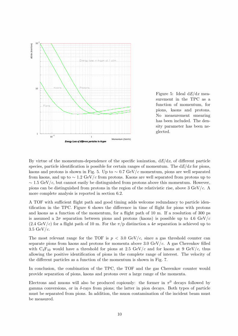
Figure 5: Ideal dE/dx mea-surement in the TPC as afunction of momentum, forpions, kaons and protons.No measurement smearinghas been included. The den-sity parameter has been ne-glected.

By virtue of the momentum-dependence of the specific ionization, dE/dx, of different particlespecies, particle identification is possible for certain ranges of momentum. The dE/dx for pions,kaons and protons is shown in Fig. 5. Up to ∼ 0.7 GeV/c momentum, pions are well separatedfrom kaons, and up to ∼ 1.2 GeV/c from protons. Kaons are well separated from protons up to∼ 1.5 GeV/c, but cannot easily be distinguished from protons above this momentum. However,pions can be distinguished from protons in the region of the relativistic rise, above 3 GeV/c. Amore complete analysis is reported in section 6.2.

A TOF with sufficient flight path and good timing adds welcome redundancy to particle iden-tification in the TPC. Figure 6 shows the difference in time of flight for pions with protonsand kaons as a function of the momentum, for a flight path of 10 m. If a resolution of 300 psis assumed a 2σ separation between pions and protons (kaons) is possible up to 4.6 GeV/c(2.4 GeV/c) for a flight path of 10 m. For the π/p distinction a 4σ separation is achieved up to3.5 GeV/c.

The most relevant range for the TOF is p < 3.0 GeV/c, since a gas threshold counter canseparate pions from kaons and protons for momenta above 3.0 GeV/c. A gas Cherenkov filledwith C4F10 would have a threshold for pions at 2.5 GeV/c and for kaons at 9 GeV/c, thusallowing the positive identification of pions in the complete range of interest. The velocity ofthe different particles as a function of the momentum is shown in Fig. 7.

In conclusion, the combination of the TPC, the TOF and the gas Cherenkov counter wouldprovide separation of pions, kaons and protons over a large range of the momenta.

Electrons and muons will also be produced copiously: the former in π0 decays followed bygamma conversions, or in δ-rays from pions; the latter in pion decays. Both types of particlemust be separated from pions. In addition, the muon contamination of the incident beam mustbe measured.

10

Pion Identification by TOFPion Identification by TOFPion Identification by TOFMomentum (GeV)

Tim

e of

Flig

ht D

iffer

ence

(ns

)

10-1

1

10

0 1 2 3 4 5 6 7 8 9 10

Figure 6: Time of flight dif-ference for pions/kaons andpions/protons as a functionof momentum for a flightpath of 10 m.

To minimize δ-rays from pions, the amount of material upstream of the gas Cherenkov countermust be kept small.

Genuine high-momentum electrons will be flagged also by 10 X0 of a lead–scintillating fibre wallfar downstream.

Muons will be identified with a sandwich of four times 10 cm of iron, interleaved with scintillatingfibres embedded in lead (75% lead) and drift chambers. Muons will thus be flagged by non-interaction in 3.4 λI.

3 Experimental setup

3.1 Beam and experimental area

It is proposed to mount the hadron production experiment in the East Hall of the PS in theT9 beam line. This beam will provide charged particles with a good momentum resolution,down to ∼ 0.24%, in the range 1.0 to 15.0 GeV/c. No particle separation is possible. Asshown in Fig. 8 there is adequate space for an experimental area of 15 × 20 m2 behind theATLAS/CMS test area. It seems desirable to be downstream of this area, because with amobile beam stopper installed at the end of the test area and in front of our system we willhave the maximum flexibility for installation and test of the experimental equipment. Therewill be no major requests from ATLAS and only a few small-scale beam tests from CMS during2000 and 2001. During 2002 there may well be requests for the assembly-area floor space forcalorimeter assembly and tests; this will need to be resolved.

Apart from the limited maximum momenta of the T9 beam, because of the magnet in the main

11

Cherenkov thresholdCherenkov thresholdMomentum (GeV)

Vel

ocity

(c

units

)

Cherenkov thresholdCherenkov threshold

0.99

0.991

0.992

0.993

0.994

0.995

0.996

0.997

0.998

0.999

1

0 1 2 3 4 5 6 7 8 9 10

Figure 7: Particle velocitiesas a function of the parti-cle momentum in the rangep GeV/c < 10 GeV/c, to-gether with the threshold forCherenkov light in C4F10.

horizontal bend, it is quite suitable for our requirements. The beam length from primary targetto the reference focus in the test area is 55.81 m. The flux of protons and pions of a few 105

per spill of 2 × 1011 protons on the primary target is adequate. The flux of low-energy kaonsis very low due to decays in this long beam line. The typical spill structure of the beam willbe a single 400 ms burst each 14.4 s cycle. The horizontal dispersion of the beam is corrected,and a typical momentum bite is 1% for a momentum collimator setting of 4 mm. The verticaldispersion is not corrected and will give some increased size to the beam spot in the target. Theextra height of the beam, 2.5 m, is also an advantage for the proposed large detector.

There are two Cherenkov counters in the beam: one 5 m long, permanently installed in the finalquadrupole doublet before the reference focus; and another, 3 m long, which can be installed infront of the focus. The Cherenkov counters are not very useful at low energies, because of thelarge multiple scattering, hence below 2 GeV/c TOF should be used instead.

Some small modifications are required to make a second focus in our area: a doublet of 1.5 mquadrupoles is placed at the end of the test area, with a new evacuated beam pipe and amodified beam stopper which can be quickly removed by the overhead crane. The spot size atour target could be of the order of 5× 5 mm2, but there are still many possibilities for furtheroptimization. The quadrupoles and power supplies are available, the other requirements aresmall. The design and construction of our target, and the final beam monitoring and triggerwill be the responsibility of the collaboration.

The power and water cooling for the TPC and spectrometer magnets are available in the EastHall. There is a single counting room available of about 30 m2. This is insufficient for theproposed experiment and an additional hut will need to be installed.

12

Figure 8: Location of the experiment in the CERN PS East Hall. The proposed experiment islocated downstream of the ATLAS/CMS area in the T9 beam line.

3.2 Overview of the spectrometer

Figure 9 shows the plan and elevation views of the experiment. Table 4 lists the various detectorsof the spectrometer. The table also summarizes the geometric envelopes of each detector alongthe beam axis (z-axis). The x-axis is defined to be horizontal, pointing to the right; the y-axis isvertical, pointing downwards. The direction of the incoming particles upstream of the target ismeasured by two small wire chambers with x and y readout planes. Several scintillation countersfor TOF and trigger purposes are placed in the beam line.

The target itself is placed in an insert at a distance of 0.5 m downstream, inside the TPC (seesection 3.4. The TPC provides dE/dx and momentum measurements of the outgoing particles.It is a 1.5 m long cylinder of 0.9 m diameter surrounded by a 1.5 T solenoid. Trigger counterssurround the TPC.

The momentum measurement of the outgoing particles is completed by the downstream spec-trometer. It comprises a quadruplet of NOMAD drift chambers before and one such quadrupletafter a large-aperture spectrometer magnet with a field strength of 1.0 Tm. All drift chambersmeasure triplets; they are described in Section 3.6. The spectrometer magnet is described inSection 3.5.

The drift chambers after the magnet are followed by a C4F10 threshold Cherenkov counter, usedto provide pion/kaon separation above 2.5–3 GeV/c (see Section 3.7).

Further drift-chamber stacks are followed by a TOF-scintillator double wall placed 10 m from thetarget (see Section 3.8). The TOF wall provides particle identification below about 4–5 GeV/c.

The TOF wall is followed by a 10.7 X0 deep electromagnetic calorimeter comprising ‘electro-magnetic’ CHORUS Pb–scintillating fibre modules [31], suitable for the rejection of electrons.

13

Table 4: Layout of the experiment; +z denotes the downstream direction; distances in metres.

From Until 〈z〉 Detector9.4 11.6 TPC solenoid flux return.9.5 10.9 TPC active volume.

10.0 Target centre (on beam axis, inside the TPC).The TPC is rotationally symmetric.Diameter 90 cm. Solenoidal field of 1.5 T.Measures r–φ and z coordinates. Particle identification by dE/dx.

11.9 12.4 12.15 Quadruplet of NOMAD drift chambers #1.12.8 14.8 13.8 ‘Orsay’ spectrometer magnet. with vertical dipole field.

The Orsay spectrometer magnet has external dimensions3.2 m hor. × 2.2 m vert. × 1.7 m depth.The magnetic gap has at present dimensions2.2 m hor. × 0.7 m vert. × 1.7 m depth.Field integral after reconfiguration 1.0 Tm.

15.3 15.8 15.55 Quadruplet of NOMAD drift chambers #2.16.0 18.5 Gas Cherenkov 2.8 m hor. × 1 m vert. entrance window18.7 19.2 18.95 Quadruplet of NOMAD drift chambers #3 and #4.19.2 19.7 19.45 Quadruplet of NOMAD drift chambers #5.

The NOMAD drift chambers #3 and #4 are arranged as a pair(side by side, although separated by a gap of 1.5 m).Drift chamber #5 is centred. The wire directionsare vertical, and +5o and −5o from vertical.

19.9 20.5 20.2 TOF walls.The TOF counter is a double-wall of scintillators of two sizes:210 × 21× 2 cm3 and 300 × 21× 2 cm3.The central area covered is 460× 300 cm2

(long counters) with two lateral pieces 140x210 cm2 (short counters) tothe left and right of the central piece. The two walls are staggered by10 cm with respect to each other to avoid loss of geometric efficiency.

20.7 23.1 21.9 Calorimeter = muon identifier.The calorimeter first consists of two layers of‘electromagnetic’ CHORUS Pb-fibre modules. Each layer has anarea of 4.96 m hor. × 3.4 m vert.Then follow four layers of 10 cm of Fe,each followed alternately with a pair of quadruplets ofNOMAD drift chambers, located side by side,and a wall of ‘hadronic’ CHORUS Pb–fibre modules.The NOMAD drift chambers cover an area of 6 m hor. × 3 m vert.The CHORUS Pb–fibre modules cover an area of8 m hor. × 3.6 m vert.The electromagnetic part comprises 6 cm of Pb (= 10.7 X0),good enough for vetoing electrons. The total number ofinteraction lengths of the calorimeter is 18 cm Pb + 40 cm Fe= 3.4 λI, suitable for muon identification.The calorimeter modules are all vertical. They are readout on either side, the vertical position is derived fromthe NOMAD drift chambers.

14

Figure 9: Plan and elevation views of the experiment. The target was arbitrarily placed atz = 10 m.

Then follow four layers of iron, each 10 cm thick. Each layer is followed alternately by a pairof quadruplets of NOMAD drift chambers, located side by side, or a plane of ‘hadronic’ CHO-RUS Pb–fibre modules. The total number of interaction lengths in both calorimeters is 3.4 λI,suitable for muon identification (see Section 3.9).

3.3 Targets

A series of target materials will be used to cover a large range of elements. The choice of thetarget materials is influenced by practical considerations. Easily machined materials in solidform have the preference.

The primary set of measurements will be performed with ‘thin’ targets. Their thickness will be2% of an interaction length. This value is chosen to minimize re-interactions in the target itself,while keeping a reasonable interaction rate. A list of target materials is given in Table 5. Thethin targets have the shape of a disc with a diameter of 30 mm and a thickness between 8.1 and1.9 mm.

A number of thick targets will be used with the primary aim of checking the simulation of re-interactions. The thickness of these targets will be of the order of one or two interaction lengths.The thickness for a one interaction length target is given in the third column of the table. Thethick targets will look like rods with up to 407 mm length. It is expected that for the thicktargets a smaller subset of materials will be used, e.g. C, Al, Cu and Pb.

15

Table 5: Set of envisaged targets. The second and third columns give the thickness of the 2%interaction length ‘thin’ version and the one interaction length ‘thick’ version respectively.

Material thin target (cm) thick target (cm)SolidBe 0.81 40.70C 0.76 38.00Al 0.79 39.44Cu 0.30 15.00Sn 0.45 22.36W 0.19 9.58Pb 0.34 17.05Cryogenic (optional)H2 14.36D2 6.76N2 2.18O2 1.59

The set of target materials can be modified to include Li, Ni, and Hg.

In a later stage, also cryogenic targets can be used, such as hydrogen, deuterium, oxygen andnitrogen. The construction of the target station with these target materials is much morecomplicated, and no design is yet available. The hydrogen target is useful to compare the resultswith earlier work. The use of the oxygen and nitrogen targets enables the direct measurement ofproduction cross-sections needed for calculations of atmospheric neutrino fluxes. A deuteriumtarget has been discussed in the framework of a recirculating proton scheme for the neutrinofactory.

3.4 Time projection chamber

The TPC has a double role in this experiment. It is used to determine the momentum of tracksgenerated by charged particles over nearly the full solid angle, with emphasis on large-angle(including the backward-going) tracks. It serves also to identify pions, kaons and protons atlow momenta. It is planned to re-utilize and suitably modify the ALEPH prototype TPC, theso-called TPC90, for the purposes of this experiment.

3.4.1 The ALEPH TPC90

The ALEPH TPC90 [9, 32] consisted of a solenoid magnet providing in pulsed mode (peakpower consumption 1.2 MW) a uniform field of 1.2 T in a volume with 90 cm diameter and1.75 m length; and of a cylindrical field cage closed with a high-voltage membrane on one side,and with a pad readout plane on the other. It was successfully operated for several years andlaid the foundations for the design and construction of the large TPC which is ALEPH’s centraldetector.

In order to re-utilize the TPC90, three major modifications are unavoidable: removing thedownstream iron end-cap of the flux return while retaining the necessary homogeneity of the

16

Figure 10: Side view of the TPC, the solenoidal magnet and the layout of the trigger detectorswith the most downstream counters in the beam. The size of the active volume of the TPC isindicated in mm. Indicated are TC-T, the target defining scintillator; FW-S and FW-C, theforward scintillator and Cherenkov counters, respectively, and BW-S and BA-S, the backwardand barrel scintillator planes, respectively. In the beam line the TOF counter BT-TOF andthe beam defining scintillator BT-B are shown. BC-D is the most downstream beam chamber.TC-T defines the effective size of the target. The beam direction is from left to right.

solenoidal field inside the TPC volume; constructing a new readout plane with circular padgeometry; and adding a small cylindrical field cage which surrounds the target inside the TPC.Since building a field cage is now a well-understood technique at CERN, rebuilding the outerfield cage is also envisaged. This would maximize the radius of the active TPC volume.

3.4.2 The solenoidal magnet

Simply removing the downstream iron end-cap of the flux return would lead to unacceptableradial field components and, as a consequence, distortions in the drift path of the charge towardsthe TPC end-plate (for optimal drifting, the electric and magnetic field vectors are parallelto each other). Therefore, the solenoidal coil as well as the cylindrical part of the iron fluxreturn must be extended at the downstream end. A programme of mapping the field in thepresent magnet configuration, and of designing the new configuration with a view to minimizingradial field inhomogeneity, has been launched. The current overall layout of the experimentassumes that a protrusion of 60 cm beyond the TPC end-plate is adequate. CERN is expectedto co-ordinate the modifications of the solenoidal magnet as well as to provide the field mapmeasurements.

The upstream end of the solenoid magnet remains unchanged.

The coil has been routinely operated in pulsed mode at 1.2 T. Given the 400 ms spill of theCERN PS and a cycle time of 14.4 s, it is quite possible that the coil can be operated in pulsed

17

mode at 1.5 T. Tests will be performed to ascertain the feasibility of this goal, taking intoaccount the limitations both from power dissipation and from magnetic field inhomogeneitiesdue to saturation in the iron flux return.

3.4.3 The TPC mechanics

The new layout of the TPC is shown in Fig. 10. The active volume is a cylinder with 42 cmradius and 140 cm length, defined by the outer field cage. The drift field is parallel to thecylinder axis, and extends from a thin membrane at the downstream end of the TPC, heldat −30 kV, to the read-out chamber which operates at ground potential. The upstream driftdirection is motivated by minimizing the material which is in the way of secondary particlesemanating from the target.

The target is located inside the TPC, 50 cm downstream of the read-out chamber, and held inposition by a suitably designed insert which can be exchanged when a new target is installed.The insert fits into the inner field cage which has a radius of 5 cm. Thus the TPC is blind toforward track segments inside a 5 cm radius.

Between the outer field cage and the solenoidal coil is a radial space of 25 mm that is used bya cylindrical array of scintillators, which permits triggering on large-angle charged particles.

The design of the pad readout is guided by the knowledge gained with the ALEPH TPC:

• A pad plane with 6 mm (azimuthally) × 15 mm (radially) pads arranged in concentriccircles between 7 cm and 40 cm radius, giving a total of ∼ 5000 pads. The pads areconnected to preamplifiers (NA49 design) which are located as close as possible to thepads.

• A sense-wire/field-wire plane with octagonal symmetry 4 mm downstream of the pad plane.The wires are not read out.

3.4.4 TPC performance

The TPC is filled with 90% Argon and 10% methane. The drift velocity is saturated at 5 cmper µs, giving a TPC cycle time of 30 µs. It is therefore the slowest detector and limits themaximum rate of the incident beam, see section 4.

An 8-bit dynamic range of the pad readout is ample.

The pad design should comfortably permit an r–φ resolution of 300 µm per pad ring. TheGluckstern formula gives, with a magnetic field of 1.5 T and 21 samplings, a pT resolution of

∆pT/pT = 0.033 pT

Along the drift direction, a sampling every cm (corresponding to a 5 MHz clock frequency) issufficient.

The greatest danger to the precision of measuring the momentum of tracks comes from residualinhomogeneities of the magnetic field. The safest way to control such problems is by using lasertracks, which have the added advantage that they not only calibrate the straightness of tracksbut also permit the linearity of the analog pad readout to be ascertained.

18

Figure 11: Top view and side view of the spectrometer magnet. All sizes are in mm.

It is envisaged that outside of run periods, the target insert will be replaced by an optical insertwhich brings in a laser beam and directs it into the active TPC volume by means of a set ofprisms which sample different polar and, by rotation, different azimuthal angles. This calls forthe optical transparency of the inner field cage at certain positions.

3.4.5 The TPC electronics

The TPC electronics is the single most demanding readout element. Every 200 ns a total of5000 analog signals must be digitized into 8-bit words and preprocessed, over 30 µs, 1000 timesper 400 ms spill, giving a raw data volume of 0.75 Gbyte. Zero suppression, which will reducethe instantaneous data volume by a factor of ∼ 100, appears mandatory.

Although very demanding and at the forefront of technology, such readout problems have beensolved already, notably by designs for the NA48 and ALICE experiments. Although the worktoward a concrete design of this experiment’s TPC readout is not finished, there is confidencethat the problem can be solved within realistic time and cost limits.

3.5 Spectrometer magnet

The track momentum measurement in the TPC is complemented by the measurement in thedownstream spectrometer. While the TPC magnet is mainly devoted to low-momentum andlarge-angle tracks, the downstream spectrometer measures high-momentum small-angle tracks.

The spectrometer magnet that we plan to use was built about 30 years ago at the Orsay labo-ratory and was previously used in PS and SPS hyperon experiments. It has a variable numberof horizontal race-track coils providing a vertical field of up to 1.5 T over a gap of 0.7 m. Thepole pieces measure 0.9 m × 1.4 m. For its previous high-momentum applications, the longerside (1.4 m) of the pole pieces was oriented parallel to the particle direction. For the proposedexperiment a large angular acceptance is of prime importance, whereas a field integral of around1 Tm is adequate. Therefore the orientation of the magnet will be changed. This orientation wasalready foreseen as an option at the time of construction of the magnet. It implies displacing the

19

vertical return yoke elements. In addition the water connections have to be renewed. Dependingon the outcome of the magnetic field calculations, a number of coils will be removed, resultingin a larger vertical gap. It is estimated that four man-months of work will be needed for thesemodifications. CERN is expected to co-ordinate the modifications of the spectrometer magnetas well as to provide the detailed field-map measurements.

Figure 11 shows the spectrometer magnet as it will be used in the experiment. The gap heightmight be further increased by removing some of the coils. The total gap width is 2.2 m. The fieldis homogeneous within 10% over a total width of 1.8 m, dropping quickly towards the sides. Thetotal depth of the magnet structure is 1.7 m. We plan to operate it at a field of 0.75 T, providinga field integral of 1.0 Tm. This gives a deflection angle of 60 mrad for 5 GeV/c particles. Theoperating values are 1600 A for a total power of 0.32 MW.

3.6 NOMAD drift chambers

The drift chambers were the active target of the NOMAD experiment and as such were more‘massive’ than ordinary drift chambers. Each chamber consists of three gas gaps (8 mm) sep-arated by 1.5 cm honeycomb-structured panels representing 2% of a radiation length for acomplete chamber. The wire orientation in NOMAD was +5◦, 0◦ and −5◦ with respect to thehorizontal direction and the cell size is ± 3.2 cm. The field shaping was designed to allow easyswitching from operation in a magnetic field (NOMAD conditions) to no magnetic field (thisexperiment). The gas mixture chosen in NOMAD was 60% ethane and 40% argon. To avoid themandatory safety aspects related to this flammable gas mixture the chambers will be operatedin a 90% argon – 5%CO2 – 5%CH4 gas mixture pending operational tests. The wire signals arefed to a preamplifier and a fast discriminator and then to a LeCroy 1876 TDC.

The typical efficiency of the chambers is 97%, most of the loss being due to the supportingrods used to maintain the 3 m long wires at the center of the gas gap. The number of deadchannels (preamplifiers or HV problems) was less than 1% in NOMAD. The average spaceresolution reached 150 µm for normally incident particles, degrading to 700 µm for 45◦ tracks.The minimum track separation is around 1 mm. More details can be found in [7]. Thesechambers are available including preamplifiers, cables and TDCs. Parts of the gas distributionsystem will have to be reconstructed.

For this experiment the NOMAD chambers have to undergo only slight mechanical modifica-tions. The small stereo angle (5◦) was chosen with respect to the magnetic field direction. Inthis experiment the chambers should be turned by 90◦ to orientate the wires vertically. The me-chanical structure used in NOMAD grouped four chambers (a module) together to ensure planarrigidity. This structure can easily be modified to provide suspension of the same four cham-bers with vertically oriented wires. These 12 active planes will then give good redundancy fortracking measurements just upstream and downstream of the spectrometer magnet. Concerningthe chambers positioned between the Cherenkov and the TOF, the three modules staggered asin Fig. 9 are designed both to cover the whole TOF acceptance (> 5 m horizontally) and toincrease redundancy in the extreme parts of the central module.

The good resolution in NOMAD came as a result of a lengthy procedure of ‘alignment’ of the6000 wires, making full use of the muon halo of the neutrino beam, thanks to the TDC ‘memory’of 64 µs. The same should be possible with the muon halo of the hadron beam, thus requiringno special trigger.

20

Acceptance region

part

icle

/pro

ton

0.02

lam

bda

Be

Acceptance region

pipl

us/k

plus

rat

io

10-7

10-6

10-5

10-4

10-3

10-2

10-1

-1 0 1 2 3 4 5

1

10

10 2

-1 0 1 2 3 4 5

Figure 12: K+ (closed cir-cles) and π+ (open circles)yields (top), and their ratio(bottom) for different angu-lar acceptance regions.

3.7 Gas Cherenkov detector

At large incident proton energy, the secondary meson and proton momenta unavoidably increase,and the particle identification capabilities of the TOF and TPC have to be supplemented byanother technique (Fig. 4). In addition to the proton/pion separation issue, the strange-particlecontamination of the pion sample also increases. By simulation, the kaon contamination is moresevere at large momenta of the secondaries, i.e. in the forward region, where the ratio K+/π+ isestimated to be about 5% (Fig. 12). In the same way, we can predict (Fig. 13) that 95% of thepions above 3 GeV/c are concentrated in the polar angle region θ < 200 mrad, and therefore the‘large momentum’ particle identification can be restricted to this domain: one obvious solutionconsists of using a gas Cherenkov detector of about 2.8 m width positioned downstream of thebending magnet. The vertical acceptance is nevertheless limited by the aperture of the magneticelement (70 cm).

A suitable gas for the radiator is C4F10 (see Table 6): It is environmentally safe, non-flammable,has a low boiling point (room-temperature operation) and has well-understood behaviour fromprevious experiments. Its high refraction index allows the radiator to be operated at atmosphericpressure and in threshold mode.

With respect to a ring imaging detector, a threshold Cherenkov detector allows for a simplerdesign and construction: fewer photo-detector channels, no need of chromatic aberration control,larger tolerances for the optical system. The light collection can be implemented by using thewell-known scheme of Al reflective mirrors: as reference, we will use the TASSO [33] design. Inthis set-up, a ‘quality factor’ of N0 = 110 cm−1 has been reached with ordinary photomultipliersand Al mirrors (no coating) in Freon 1141.

1Chlorofluorocarbons can no longer be used, and have to be substituted by equivalent perfluorocarbons.

21

Polar angle distribution of pions above 3 GeVpolar angle (rad)

a.u.

Integral Polar angle distribution of pions above 3 GeVpolar angle (rad)

a.u.

0

250

500

750

1000

1250

1500

1750

2000

-0.1 0 0.1 0.2 0.3 0.4 0.5 0.6 0.7 0.8

0

0.2

0.4

0.6

0.8

1

-0.1 0 0.1 0.2 0.3 0.4 0.5 0.6 0.7 0.8

Figure 13: Angular dis-tribution of positive pionswith momentum larger than3 GeV/c (top). The integraldistribution is shown below.

Table 6: C4F10 chemical/physical characteristics

Boiling point (◦C) −2Molecular weight (g/mol) 238.0(n − 1)× 106 1415γthr 18.8Pion threshold (GeV/c) 2.6Kaon threshold (GeV/c) 9.3Proton threshold (GeV/c) 17.6θmaxc (mrad) 53d2N/dxdE (photons/cm/eV) 1.04

The subdetector could be made by 16 identical modules with an input window of 35 × 50cm2, positioned symmetrically with respect to the horizontal plane to cover a surface of 280 ×100 cm2 (Fig. 14). Each module contains a single mirror and a 5” photomultiplier. The mirrorhas an ellipsoidal shape with the photomultiplier and the target at focal points. Clearly, themagnetic fields will introduce distortions in the particle trajectories, resulting in a larger angulardistribution of the particles entering one Cherenkov module. The actual angular acceptance ofthe single module (10◦ in the horizontal plane for the TASSO design) has to be optimized by aMonte Carlo study of the magnetic fields vs. mirror focal length. It has to be noted, however,that a larger angular acceptance can be reached by using 20” photomultipliers (commerciallyavailable) that have a photo-cathode surface 16 times larger. A minimum radiator depth of about150 cm allows the detector to be operated in safe conditions, since about 40 photoelectrons canbe expected for a relativistic particle (Fig. 15). The large photostatistics also allows pions and

22

Figure 14: Sketch of a sin-gle Cherenkov detector mod-ule (left), and top and lateralview of the complete detec-tor (right).

C4F10 emissionMomentum (GeV)

Exp

ecte

d ph

otoe

lect

rons

/cm

C4F10 emission

0

0.05

0.1

0.15

0.2

0.25

0 2 4 6 8 10 12 14 16 18 20

Figure 15: Photoelectronyield on photomultipliermeasured in the TASSOCherenkov detector nor-malized to 1 cm of radiatorlength. Both pion andkaon momentum curves arereported.

kaons to be discriminated above 9 GeV/c, by selecting on the intensity of the signals accordingto the momentum of the particle.

3.8 Time-of-flight wall

In the proposed design of a time-of-flight (TOF) system it is envisaged to use the scintillatorsthat were used for the TOF system [34] of the Grenoble n–n experiment [35]. Part of these

23

Figure 16: Conceptual lay-out in plan view of the muonidentifier. Sizes are indicatedin m.

scintillators were subsequently re-used in the NOMAD veto system [36].

The plastic scintillator used is NE110 manufactured by the former Nuclear Enterprise, UK.There are two types of counters: 28 slabs of 210× 21× 2 cm3 and 46 slabs of 300× 21× 2 cm3,all equipped with light guides and Philips XP2020 photomultipliers at both ends. The slabs arewrapped in a thin aluminum sheet and in black plastic. A small prism is glued to the centreof each scintillator. It allows connection to an optical fiber that can be used for an externaltiming monitoring system. Such a monitoring system, needed for this experiment, is no longeravailable and must be rebuilt. A specially designed mean-timer [37] can be used to build triggersignals for the experiment.

The time resolutions of the scintillator counters [34] were 270 and 320 ps, on average, forthe 2.1 and 3.0 m long counters, respectively. The attenuation length was ∼ 350 cm. Theseperformances were obtained with cosmic-ray measurements. Leading-edge discriminators wereused and no correction for time walk effect was applied.

With these scintillation counters two walls of 20 m2 can be equipped. The expected time resolu-tion is already suitable to separate with 4σ pions from protons up to 3.5 GeV/c on the basis of10 m flight path. We expect to improve the original resolution by using the amplitude measuredby ADCs and combining the signals of the two consecutive planes. Also constant-fraction dis-criminators can be used. These techniques can help to improve the pion/kaon separation in the1.5–3.0 GeV/c range and provide a useful overlap with the other particle identification methods.

3.9 Muon identifier

At low energies of the secondary pions and kaons the decay-in-flight probability will be important(∼ 5% for pions and ∼ 40% for kaons of 2 GeV/c momentum).

24

Table 7: Parameter list of the beam and DAQ

Parameter Estimated valueEvent readout time 300 µsLength of PS spill 400 msMaximum number of events per spill 1334Length of super-cycle 14.4 sNumber of spills per day 6000Maximum beam intensity (protons/spill) 3× 105

Worst case π/beam particle 2× 10−3

Required statistics per setting 5× 106

Number of settings ≈ 140

The decay of these particles produces the following effects:

• wrong pL and pT assigment;

• the decay of a pion in the Cherenkov detector will increase the TOF so producing a possiblepion/kaon confusion.

Although these effects can be corrected on a statistical basis, muon identification on an event-by-event basis would be helpful also for solving problems of pattern recognition.

The quantitative importance of the above-mentioned effects is under study, as is the design ofan efficient muon identifier. It must be recalled that the pion/muon separation is non-trivial astowards low-momentum pions increasingly look like muons in the passage through matter.

A possible design is shown in Fig. 16. The design is largely driven by the re-use of existingequipment. After a double-wall of the 4 cm thick CHORUS Pb–scintillating fibre modules(10 X0) [31] that will also act as veto for electrons, a structure consisting of four times 10 cmFe, interspersed alternately with a quadruplet of NOMAD drift chambers (side by side) and awall of 8 cm thick CHORUS Pb–scintillating-fibre modules will permit hadrons to be separatedfrom muons at the ∼ 90% level.

The central part of the muon identifier is needed to detect muons in the incident beam. Thesehave higher momenta than the particles produced in the interactions in the target. An extensionof the muon identifier with a limited lateral size is envisaged making use of existing scintillatorplanes and iron pieces.

4 Trigger

The design of the trigger is driven by the capabilities of the data-acquisition system (DAQ), theperformance and properties of the beam, the main features of the interactions to be studied andthe required precision of the measurement envisaged. We will first make a rough survey of theconditions under which the trigger operates.

25

4.1 Running conditions

A list of parameters defining the running conditions is given in Table 7.

The secondary beam from the PS has a spill length of 400 ms with a repetition rate of onespill every super-cycle of 14.4 s. The intensity of the secondary beam varies depending on themomentum setting of the secondary beam line. By adjusting the collimators in the line andvarying the production targets it will be possible to obtain particle rates of 105 to 3 × 105 forall energies. The beam on the target of the experiment will be focused to contain at least 90%of the intensity within a spot size of 10 mm diameter.

The optimum intensity of the secondary beam is limited by the occupancy of tracks in the TPC.The maximum drift time of the electrons in the TPC is 30 µs. The through-going beam particlestraverse a dead zone in the TPC volume which is shadowed by the target cylinder. If the beamintensity is adjusted to give a maximum of 6000 interactions per spill (2% interaction lengthwith 3 ×105 intensity), the overlap probability in the TPC is 0.6. It is expected that constraintson the interaction point provided by the beam chambers and combination with faster detectorsdownstream can resolve the ambiguities. In other detectors, the time windows are considerablysmaller and the occupancy is negligible, except for the region traversed by the incident beam.

The number of random coincidences in the trigger should be kept at a reasonable level. Withan intensity of 3 × 105 protons in a 4 × 102 ms spill time the random coincidence rate in a10 ns trigger time window is less than 1%.

Acceptance region

part

icle

/pro

ton

0.02

lam

bda

Be

Acceptance region

prot

on/p

iplu

s ra

tio

10-4

10-3

10-2

10-1

-1 0 1 2 3 4 5

10-1

1

10

-1 0 1 2 3 4 5

Figure 17: π+ (open circles)and proton (closed circles)yields (top), and their ratio(bottom) at 2 GeV/c inci-dent momentum for differentangular acceptance regions.

The characteristics of the interactions vary greatly over the energy range of the experiment. Athigh energy, pion and proton production rates are roughly equal. Since both measurements arerequired, no selection on particle type will be needed in the trigger. At low-momentum settings

26

(below 4 GeV/c) the proton production dominates (Fig. 17). This effect is most marked in anangular range between 5 and 30 degrees. Therefore an additional trigger condition is requiredin this angular range to enrich the data with pion production.

To explore the two-dimensional phase space in transverse and longitudinal momentum with astatistical accuracy of 1% in the relevant area, 5 ×106 events are required for each of the roughly140 different settings (targets and momenta). To limit the measurement time to one year, oneshould aim at obtaining the statistics for each setting within one day, perhaps with the exceptionof the most difficult low-energy settings.

At low energy, the number of interaction triggers is low compared to the number of incomingbeam particles. A decision dead time of 60 ns seems achievable, and gives a loss of 5% for 3 ×105

incoming beam particles in a 400 ms spill.

The performance of the DAQ can only be determined with precision once a full design of allconversion electronics is available. It is estimated to be around 300 µs. Its effect on the numberof events recorded is shown in Fig. 18.

1

10

10 2

10 3

1 10 102

103

104

105

106

Interaction rate [events / spill]

Eve

nts

rec

ord

ed

100 µs

200 µs

300 µs

Interaction rate [events / spill]

Fra

ctio

n o

f ev

ents

rec

ord

ed

10-2

10-1

1

1 10 102

103

104

105

106

Figure 18: The effect of theread out time on the num-ber of recorded events perspill (left) and the numberof ‘effectively used’ triggers(right). The calculation isdone for three values of theread out time (100, 200 and300 µs). The spill durationis 400 ms.

4.2 Trigger layout

The trigger counters can be separated in three groups: the counters in the secondary beam line,near the TPC and downstream of the dipole magnet.

A large angular acceptance is achieved by combining a barrel-shaped system around the TPCvolume with a planar system in the forward and backward direction. The various systemswill have overlapping acceptances to allow a cross-check of the trigger efficiencies. The planardetectors have holes at the position of the beam spot to avoid triggering on non-interacting

27

beam particles. In low-energy incident beams up to 4 GeV/c it is important to distinguish pionsfrom low-energy protons at the trigger level. Such suppression of proton triggers is only neededin a limited angular region (5 to 30 degrees). The use of a solid radiator such as quartz orlucite ensures the suppression of these protons. A thickness of 10 mm of quartz with a standardcollection efficiency gives a comfortable number of 30 detected photoelectrons [38].

A series of scintillation counters is placed in the incident beam line (Fig. 10). A scintillationcounter is used to give a precise timing for the TOF system BT-TOF. It has to be rather thick(∑

20 mm) for good timing resolution, and is therefore positioned far upstream of the targetto avoid secondary particles faking a good trigger. A beam-defining scintillator is closer to thetarget. This counter is thin and has a circular shape of the size of the cylindrical free spacearound the target BT-B.

Beam chambers (BC-U, BC-D) are placed upstream and downstream of the scintillation coun-ters, with the aim to measure the direction of the incoming beam within 1 mrad. The positionresolution is about 1 mm projected onto the target. The precision of these detectors will makeit possible to disentangle overlay beam tracks from the interacting beam particle.

A number of trigger elements are positioned inside the TPC magnet. These detectors are shownin Fig. 10.

The main trigger elements inside the TPC magnet are the scintillator layers BA-S and BW-S.The barrel shaped BA-S covers the large-angle region, partly including backward particles. It isread out with light-guides in the downstream direction. It gives a simple large-angle interactiontrigger. The planar system of scintillators, BW-S, is fixed upstream of the TPC inside theMagnet yoke. The light is transported out of the barrel through the slits in the yoke withlight-guides. A hole in this plane allows the beam to pass.

To trigger on forward produced particles, planar detectors are used immediately downstream ofthe magnet return yoke. A set of solid Cherenkov counters (FW-C) and scintillation counters(FW-S) is used. They cover at least the 90 cm diameter end-face of the TPC. The non-interacting beam particles pass through a ∼ 120 mm diameter hole in the middle of thedetectors. A side view is given in Fig. 10. Light-guides carry the light sideways out of the fringefield of the solenoid. The Cherenkov has the function to discriminate protons from pions upto about 800 MeV/c, and is made of 10 mm quartz or lucite plate. It is only needed at lowenergies, and can be removed in higher-energy runs.

An array of planar scintillation detectors (SA-S) downstream of the dipole magnet definestriggers by detecting small-angle particles. These counters are located close to the TOF detectorsshown in Fig. 9. They cover the diameter of the hole in the forward planar detectors withconsiderable overlap to allow for the effect of the bending field of the dipole magnet. Dependingon the beam setting, a counter in the middle of the array is hit by the non-interacting beamparticles and is not used in the coincidence. A selection of the TOF counters can be used forthis function, perhaps complemented by a number of horizontal scintillator strips to improvethe geometrical coverage at the centre, where the beam spot has to be blanked out.

4.3 Trigger conditions

In runs with thin targets the trigger requires a beam particle (BT-TOF × BT-B × TC-T) anda positive indication of an interaction, by defining an off-axis hit in any of the other scintillatorplanes. At low-energy running an additional Cherenkov signal is required in the forward region.

28

Table 8: Preliminary cost estimate of the data acquisition (in kCHF)

Item Quantity Unit price TOTALSVME crates 11 10 110VME/PCI interfaces 11 5 55DAQ-PCs 11 3 33Local disk buffer 1 15 15EVB/database PCs 5 3 15Number crunching PCs 5 3 15Control PCs 5 2 10Monitoring PCs 5 2 10Monitors 12 2 24Network switches 2 4 8Console switch 1 5 5

TOTAL 300

During data-taking with thick targets, most beam particles interact. It is not necessary to definesophisticated triggers, and a simple incoming beam trigger suffices. Also during operation withthin targets, it is important to have triggers defined with low-bias conditions. It is alwaysforeseen to have a down-scaled incoming beam trigger and to have a trigger without the solidCherenkov conditions with a lower down-scale factor. In the high-energy incoming beam settings,triggers without Cherenkov thresholds applied will be used without down-scaling.

5 Data acquisition and computing

5.1 Introduction

The data-acquisition system (DAQ) will read out the digitized signals from the ADCs and theTDCs. The DAQ will also take care of storage of the data in the proper sequence and format, thecalibration of the detector and of the electronic readout chain, and the overall synchronization ofthe readout processes. It will also include slow control and data quality monitoring. The designaim for the DAQ is to keep the total dead time below 300 µs. A preliminary cost estimate isgiven in Table 8.

5.2 Readout and data volumes

An overview of the readout configuration is shown in Fig. 19. VME crates will be used whereverpossible. The only exception to this rule will be the readout of the NOMAD drift chambers.The existing electronics in the FASTBUS standard will be re-used; in this case the FASTBUScrates will be interfaced to VME. Each VME crate will be connected to a readout PC via aVME–PCI interface.

64 channel ADC and TDC 9U VME modules will be used to read out the TOF system, thetrigger system, the beam chambers and the gas Cherenkov detectors; these modules cannot be

29

FRONT-END ELECTRONICS

VME/PCI

CA

LIB

RE

CO

NS

SWITCH

SWITCHFASTETHERNET

MONITORING WORKSTATIONS

REMOTE DATA RECORDINGTO DB SERVERS OR

EV

B

DIS

PAT

CH

ER

S

ADCs TDCs

DAQ-PCs

MAIN

VME BUS

CONTROL ROOM

CERN-WIDE NETWORK

Figure 19: Schematic layout of dataacquisition and networking.

recuperated from previous experiments and must be purchased.

All the necessary 96 channel FASTBUS TDC modules (LeCroy model 1876) needed for theNOMAD drift chambers are still available. These modules are equipped with an on-board64 kB buffer memory and on-the-fly zero suppression [7].

A special case is the readout of the TPC, where we will use custom-made ADC modules developedin the framework of the ALICE TPC R&D programme. Up to 48 input channels per board maybe sampled in parallel at 10 MHz with on-the-fly zero suppression and storage in a memorybuffer [39]. We will operate these at 5 MHz. Approximately 100 modules will be needed to readout the TPC; of these, approximately 30 are already in existence and enquiries are being madeto explore the possibility to borrow them, while the others have to be produced.

All the ADC and TDC modules will provide one data word per channel. All the data wordswill be 4 bytes long. Present tests of VME-PCI links show that the bandwidth in block transfermode exceeds 10 Mbytes/s; conservatively assuming this data rate, keeping the readout timebelow 250 µs requires that no more than ∼ 620 words per VME crate have to be read out perevent. These parameters have been used to determine the number of crates and DAQ-PCs thatare necessary to build the DAQ system fulfilling the dead-time requirements.

The drift chamber system will be read out following the scheme already used in NOMAD: Ateach incoming trigger the zero suppression is performed by the TDC modules and the survivinghits stored in their memory buffer, which is then read out after the end of the spill. This ensuresan almost dead-timeless operation of the drift chambers. The data volume produced by the TPC

30

is huge. Before any zero suppression, the TPC produces 150 samples per channel, correspondingto a total of 0.75 million samples. However, since the events have a low multiplicity, a largezero suppression factor can be achieved (a few 102) and a fast event-by-event readout (in lessthat ∼ 250 µs) will be possible. All the remaining detectors will be read out for each eventwithout applying any zero suppression. All the data read out during the spill will be stored inthe DAQ-PCs memory.

At the end of the spill all the data will be transferred in parallel to a dispatcher PC throughEthernet links. The dispatcher concept has already been successfully used by the CHORUScollaboration for DAQ environments, both inside and outside CERN [40]. The bandwidth offast-Ethernet (100 Mbit/s) switches ensures that the data from the whole experiment (∼ 26Mbyte) will be transferred in ∼ 3 s. The spare time will be used by the DAQ-PCs to acquirecalibration events.

Assuming 100% efficiency and 200 days running, the total yearly data volume would be approx-imately 30 Tbyte. Central recording at the computer centre of these data will be required. Adisk buffer will be used to store the data of about four days running locally. Disk space fortemporary data storage is also needed at the computer centre.

5.3 Network topology

The network will be organized around two Ethernet switches as in Fig. 19. The driving idea isto have a switched fast-Ethernet (100 Mbit/s) backbone dedicated to the critical tasks, and toscreen anything else behind a second switch.

The readout PCs will be connected to the main switches to take advantage of the fastest possiblenetwork speed.

Direct connection on the main backbone is foreseen for all the PCs that require the highestpossible throughput and the minimum possible latency. These machines will most likely be thereadout processors, the dispatcher, the event builder (EVB), the calibration processors, the runcontroller and the file/database server.

To isolate the DAQ traffic which has the highest priority, the monitoring tasks will be run onworkstations connected to the backbone via a fast-Ethernet switch. The link to the CERN-widenetwork will also be connected to the switches. Unnecessary traffic from the outside will haveto be screened at the switch.

6 Performance of the spectrometer

AMonte Carlo simulation of the proposed experiment has been carried out using the GEANT [41]package, with the FLUKA [42] interface for the hadronic interactions. As examples of the ex-pected performance, data with 2 GeV/c and 15 GeV/c protons impinging on a beryllium targetwith 2% λI thickness have been simulated.

The geometry and positioning of each of the subdetectors in the simulation is as described inTable 4 and as shown in Fig. 9. In a first stage of the simulation, tracking of all particlesis carried out in each of the subdetectors with the position, momenta and identity of all theparticles recorded. In a second stage, all particle detection effects such as momentum smearingand particle identification are simulated.

31

pion distribution for 2 GeV protons on beryllium target (GFLUKA)pion distribution for 2 GeV protons on beryllium target (GFLUKA)Longitudinal Momentum (GeV/c)

Tra

nsve

rse

Mom

entu

m (

GeV

/c)

0

0.1

0.2

0.3

0.4

0.5

0.6

0.7

0.8

-0.5 -0.25 0 0.25 0.5 0.75 1 1.25 1.5 1.75 2

proton distribution for 2 GeV protons on beryllium target (GFLUKA)proton distribution for 2 GeV protons on beryllium target (GFLUKA)Longitudinal Momentum (GeV/c)

Tra

nsve

rse

Mom

entu

m (

GeV

/c)

0

0.1

0.2

0.3

0.4

0.5

0.6

0.7

0.8

-0.5 -0.25 0 0.25 0.5 0.75 1 1.25 1.5 1.75 2

Figure 20: Production spectrum (by GEANT+FLUKA) d2N/dpT dpL of (left) secondary pionsand (right) secondary protons produced in collisions of protons of 2 GeV/c with a thin berylliumtarget. Superimposed are the areas of phase space expected to be covered by the π/p particleidentification of the TPC and the TOF (at the 4σ level) in a simplified treatment.

pion distribution for 15 GeV protons on beryllium target (GFLUKA)pion distribution for 15 GeV protons on beryllium target (GFLUKA)Longitudinal Momentum (GeV/c)

Tra

nsve

rse

Mom

entu

m (

GeV

/c)

0

0.1

0.2

0.3

0.4

0.5

0.6

0.7

0.8

0.9

1

0 1 2 3 4 5 6

proton distribution for 15 GeV protons on beryllium target (GFLUKA)proton distribution for 15 GeV protons on beryllium target (GFLUKA)Longitudinal Momentum (GeV/c)

Tra

nsve

rse

Mom

entu

m (

GeV

/c)

0

0.1

0.2

0.3

0.4

0.5

0.6

0.7

0.8

0.9

1

0 2 4 6 8 10 12 14

Figure 21: Production spectrum (by GEANT+FLUKA) d2N/dpT dpL of (left) secondary pionsand (right) secondary protons produced in collisions of protons of 15 GeV/c with a thin berylliumtarget. Superimposed are the areas of phase space expected to be covered by the π/p particleidentification of the TPC and the TOF (at the 4σ level) in a simplified treatment. The combinedanalysis explained in the text gives better results.

32

Figure 22: Truncated mean(40%) of the ionization loss(in arbitrary scale) of pi-ons, kaons and protons in theTPC from 15 GeV/c protonson a Be target.

6.1 Momentum measurement

The momentum smearing inside the TPC is applied with the resolution given by the Glucksternformula. The resolution of every r–φ measurement is assumed to be 300 µm, and the magneticfield is 1.2 T. A track is considered measured in the TPC when its projection onto the end-platehas a length greater than 15 cm.

For the momentum measurement in the spectrometer magnet, we use a quadruplet of NOMADdrift chambers before and after the magnetic volume. These drift chambers have a resolution ofbetter than 250 µm, but they add 8% of a radiation length. In this case, the multiple scatteringerror dominates.

6.2 Particle Identification

To understand the particle identification capabilities of the TPC we assume a measurement ofthe ionization every cm. For the purpose of the simulation it is sufficient to assume that thegas is pure argon. To compute the ionization loss I = dE/dx for each track we determine thetruncated mean (at 40%) of the measurements. Fig. 22 shows the truncated mean (at 40 %) ofthe computed ionization loss I = dE/dx for each track of the measurements.

The time of flight of a particle is calculated from the physical track length of a particle. It hasbeen shown that a π/p separation can be achieved up to about 3.5 GeV/c at the 4σ level and aπ/K separation up to about 2.5 GeV (at 2σ). The effective time resolution of the measurementof the TOF was assumed to be ∼ 300 ps.

We assume a very similar performance for the threshold Cherenkov counter to the performanceof the TASSO Cherenkov detector [33]. The pion identification efficiency drops rapidly below3 GeV/c towards the threshold at 2.5 GeV/c. Above 3 GeV/c, pions are identified with anefficiency close to 100%.

33

Figure 23: Acceptance of the detector for pions produced by a proton beam of 15 GeV/c incidentmomentum on Be measured in (left) the TPC and (right) the magnetic spectrometer.

Figure 24: Combined accep-tance for pions produced bya proton beam of 15 GeV/cincident momentum on Bemeasured either by the TPCor the magnetic spectrome-ter.

6.3 Results of the simulation

6.3.1 Geometrical acceptance

Figs. 20 and 21 show the distribution of events in the transverse–longitudinal momentum plane(d2N/dpT dpL) for the secondary pions and protons produced in the interactions with a thinberyllium target of 2 GeV/c and 15 GeV/c protons, respectively.

Overlayed on those plots one can see the approximate regions of parameter space covered bythe π/p identification capabilities of the TPC and the TOF. At 2 GeV/c there is total particle

34

Figure 25: Combined accep-tance for pions produced bya proton beam of 2 GeV/cincident momentum on Bemeasured either by the TPCor the magnetic spectrome-ter.

identification coverage for all pions and nearly all the protons.

At 15 GeV/c the π/p separation can also be achieved unambiguously for most of the phase space.Here a simplified particle identification in the TPC was assumed, limited to the momentumregion below the crossing points of the ionization curves (Fig. 5). As will be demonstrated insection 6.3.3 good identification of pions can also be achieved with the dE/dx in this region. Atthis momentum there seems to be a small area between 2.5 and 3 GeV/c where π/K separationcannot be achieved unambiguously when one uses a particle identification in the TPC limited tothe momentum region below the crossing points of the ionization curves. Sufficient identificationcan be achieved in this region on a statistical basis (section 6.3.3).

Fig. 23(left) shows a three-dimensional plot of the pL–pT-plane in which the third coordinate isthe acceptance of the TPC for pions produced by 15 GeV/c incident protons. This is defined,for each event, as the number of pions which are triggered (that is, they hit at least one of thetrigger scintillators) and tracked by the TPC (the projected length in the TPC end-plate mustbe longer than 15 cm), divided by the total number of produced pions. Fig. 23(right) shows thesame plot for the magnetic spectrometer, while Fig. 24 shows the combined acceptance. Thisacceptance is purely geometrical. The acceptance of pions over the full phase space is almost100%.

Similarly, one can show in Fig. 25 the same geometrical acceptance plot for pions from protons of2 GeV/c. The geometrical coverage between the TPC and the rest of the magnetic spectrometeris nearly complete.

6.3.2 Particle identification efficiency

For each of the subdetectors with particle identification characteristics, we compute the proba-bility that a particle is a pion, kaon and proton. For example, the probability that a particle is apion in the TPC, P π

TPC(I, p), is a function of the measured ionization and its momentum. We alsodefine the pion identification efficiency as the number of correctly identified pions divided by theinitial number of pions tracked by the TPC (so that we deconvolute the identification efficiencyfrom the geometrical acceptance). We also calculate the kaon (proton) relative misidentification

35

Figure 26: (left) Combined pion identification and geometrical acceptance of the detector and(right) global pion misidentification probability in bins of pL, pT from interactions of 15 GeV/cprotons.

probabilities, as the number of kaons (protons) wrongly identified as pions divided by the initialnumber of kaons (protons) tracked by the TPC. Finally, we compute an absolute misidentifica-tion probability as the number of kaons plus the number of protons wrongly identified as pionsdivided by the initial number of pions. This latter quantity is a direct measure of the backgroundin our sample of pions.

With a choice of P πTPC(I, p) > 0.6, one keeps a pion identification efficiency of 92%, while

reducing the absolute misidentification probability to about 0.4%.

Also defined is the probability that a particle is a pion, P πTOF(t, p), which depends on the time of

flight (in ns) and its momentum. We repeat the same likelihood analysis with the TOF and witha choice of P π

TOF(t, p) > 0.5, one keeps a pion identification efficiency of 79%, while reducing theabsolute misidentification probability to about 0.6%.

6.3.3 Combined Acceptance and efficiency

The combination of the geometrical acceptance and the particle identification efficiencies of theTPC, TOF and Cherenkov yields the combined acceptance. At this stage, we have applied verysimple criteria, which we summarize as follows:

1. If the particle has p > 3 GeV/c and the track length in the Cherenkov is longer than1 m we assume it can be identified in the Cherenkov with 100% efficiency. This is a goodapproximation of the efficiency of a threshold Cherenkov detector.

2. If the particle has p < 3 GeV/c and reaches the TOF, then it is identified as a pion ifP π

TOF(t, p) > 0.5.

3. Else, if the particle has been tracked by the TPC, then it is identified as a pion if

36

Figure 27: Combined pionidentification and geometri-cal acceptance of the detec-tor in bins of pL, pT frominteractions of 2 GeV/c pro-tons.

P πTPC(t, p) > 0.6.

Fig. 26 shows the combined pion acceptance plus identification efficiency as a function of pL, pT

and the pion misidentification probability as a function of the same variables from 15 GeV/cprotons. The identification and measurement of pions is achieved with a high efficiency (90%)while maintaining the contamination from other particle types as low as 0.2 %.

For completeness we also show in Fig. 27 the combined pion acceptance plus identificationefficiency as a function of pL, pT for 2 GeV/c protons. The misidentification probability istotally negligible while the pion acceptance is very close to 100%.

To illustrate the performance of the apparatus we show in Fig. 28(a) the momentum distributionfor pions (solid), protons (dashed) and kaons (dotted), produced by 15 GeV/c protons (i.e, the‘true’ Monte Carlo distribution). The effect of the acceptance in these distributions can be seenin Fig. 28(b) while the effect of particle identification is shown in Fig. 28(c). The efficiency forsignal and background is shown in Fig. 28(d). Coverage down to very low momenta is clearlyobtained with the proposed apparatus. Even though the identification efficiency is somewhatreduced in the 1–3 GeV/c region, it is still possible to separate pions from other particles witha low background of misidentified particles.

As expected at 2 GeV/c incident proton momentum, the same analysis confirms that the effi-ciency for measurement and identification is practically 100%

7 Cost estimate

The estimated cost of constructing, installing and commissioning the experiment is given inTable 9. The cost of digitization electronics (ADCs and TDCs) and of cabling are reportedseparately. Some items can be reduced if more existing equipment can be re-used.

37

Figure 28: Momentum distribution for pions (solid line), kaons (dashed line) and protons (dottedline) produced in p–Be collisions at 15 GeV/c. (a) ‘True’ distribution, without convoluting withthe geometrical acceptance and the particle identification; (b) the same distribution when thegeometrical acceptance is included; (c) the same including the effect of particle identification(the background due to misidentified protons and kaons is shown with dotted and dashed linesrespectively); and (d) final efficiency (acceptance and particle identification).

8 Schedule

From the point of view of the knowledge of the atmospheric flux, there is no specific timetableimposed, except that sooner is better than later.

From the point of view of the neutrino factory, there is an important choice to be made inthe not–too–distant future. The two proposed extremes are a superconducting proton linac

38

Table 9: Cost estimate of the experiment construction (in kCHF)

Item Cost Digitization CablesSecondary beam upstream of the experiment’s target 50(beam focus, particle id., T9 beam stopper)Beam chambers (mechanics, electronics) 10 24 4Targets and associated mechanics support 50Trigger counters 150 12 10(including support structures, logic, distribution)TPC field cages, pad readout chamber 300TPC readout (preamplifiers) 100 300 100TPC solenoid magnet 100(coil extension, reshaping of flux return, installation)Spectrometer magnet 60(modification and installation)NOMAD drift chambers 150(mechanical supports, refurbishing)Gas distribution systems 100(for TPC and drift chambers)Gas Cherenkov 350 2(mechanical structure, mirrors, PMs, gas system)TOF walls 160 30 10(construction, mechanical supports, calibration system)Muon identifier/ calorimeter 100 90 30(mechanical supports, installation)Data acquisition 300(crates, processors, servers, work stations, slow control)Network connections 40Offline analysis infrastructure 50Experimental area 50(installation of infrastructure, access ways, cable trays, etc.)Experimental huts 100(installation incl. electronics racks and cooling)Electrical power distribution 50Safety equipment 100Installation manpower 300(three man-years, including a designer for six months)Subtotals 2670 458 154Total 3282

producing 2 GeV/c protons, or else a rapid-cycling synchrotron producing 16 GeV/c protons. Ifthe decision is to be taken on the basis of measured data, they should become available as soonas possible.

Another constraint is the availability of the East Hall of the CERN PS for a large experiment,since the room is dedicated for later use by LHC experiments.

Therefore, the plan is to install and commission the experiment as rapidly as possible, with a

39

view to having a technical run in late 2000. The main data-taking period would be 2001. Theoption of a second data-taking period in 2002, with deuterium and helium running, should bekept open.

Acknowledgements

The authors wish to express their sincere thanks to all members of the Neutrino Factory Work-ing Group for their advice and assistance: in particular to B. Autin, H. Haseroth, E. Keil andE.J.N. Wilson; and to R. Engel, T.K. Gaisser, J. Knapp, P. Lipari and A.A. Watson for valuablediscussions on charged-particle cosmic rays. We are indebted to W. Blum for sharing his exper-tise of the TPC and to G. Mallot for the information on COMPASS. We greatly acknowledgethe contributions from the staff of the PS division concerning information on the T9 beam pa-rameters and infrastructure. We warmly thank the technical staff of the collaborating instituteswho have contributed to the preparation of the proposal.

References

[1] Y. Fukuda et al. (SuperKamiokande Collaboration), Phys. Lett. B433 (1998) 9;Phys. Rev. Lett. 81 (1998) 1562.

[2] T. Kajita, Nucl. Phys. B77 (1999) 123.

[3] J.V. Allaby et al., CERN report 70–12 (1970).

[4] T. Eichten et al., Nucl. Phys. B44, (1972) 333.

[5] B. Cole et al., BNL Proposal 910 (1994), AGS propsal: “A Facility to Study Proton-nucleusand Heavy Ion Collisions using a Large Acceptance Detector with Particle IdentificationCapabilities.”

[6] I. Chemakin et al., preprints nucl–ex/9902003 and nucl–ex/9902009 (1999).

[7] J. Altegoer et al. (NOMAD Collaboration), Nucl. Instrum. Meth. A404 (1998) 96.

[8] E. Eskut et al. (CHORUS Collaboration), Nucl. Instrum. Meth. A401 (1997) 7.

[9] S.R. Amendolia et al., Nucl. Instrum. Meth. A252 (1986) 392.

[10] J.P. Riunaud, private communication.

[11] B. Autin et al., Prospective study of muon storage rings at CERN, CERN 99-02 (1999).

[12] D. Harris et al., Summary of detector/neutrino beam parameters. talk at Nufact’99 in Lyon,to be published in Nucl. Instrum. Meth.

[13] R. Palmer et al., Draft parameters of a neutrino factory, Muon Collider Note 46.

[14] R. Palmer, C. Johnson and E. Keil, A cost effective design for a neutrino factory. talk atNufact’99 in Lyon, to be published in Nucl. Instrum. Meth.

[15] J. Collot et al., Particle production comparisons between MARS, FLUKA and E910, talkat Nufact’99 in Lyon, to be published in Nucl. Instrum. Meth.

40

[16] A. Blondel et al., A thin target scheme for the muon source, talk at Nufact’99 in Lyon, tobe published in Nucl. Instrum. Meth.

[17] V. Agrawal et al. (Bartol group), Phys. Rev. D53 (1996) 1314.

[18] M. Honda et al. (HKKM group), Phys. Rev. D52 (1995) 4985.

[19] E.V. Bugaev and V.A. Naumov (BN group), Phys. Lett. B232 (1989) 391.

[20] D. Perkins, Astrop. Phys. 2 (1994) 249.

[21] G. Battistoni et al., preprint hep–ph/9907408 (1999), to appear in Astrop. Phys.

[22] Y. Tserkovnyak et al., preprint hep–ph/9907450 (1999).

[23] T.K. Gaisser et al., Phys. Rev. D54 (1996) 5578.

[24] T.K. Gaisser, talk given at the TAUP’99 Conference, Paris (France), September 1999.

[25] M. Honda, Nucl. Phys. B77 (1999) 140.

[26] R. Bellotti et al. (MASS Collaboration), Phys. Rev. D53 (1996) 35; R. Bellotti et al. (WiZ-ard/MASS2 Collaboration), Phys. Rev. D60 (1999) 052002.

[27] M. Boezio et al. (CAPRICE Collaboration), Ap. J. 518 (1999) 457.

[28] T. Sanuki et al. (BESS Collaboration), Proc. 26th Int. Conf. on Cosmic Rays, Salt LakeCity (USA, August 1999), Vol. 3 (1999) 93.

[29] R. Engel, T.K. Gaisser and T. Stanev, Bartol preprint BA–99–73 (1999).

[30] T. Abbott et al., Phys. Rev. D45 (1992) 3906.

[31] E. Di Capua et al., Nucl. Instrum. Meth. A378 (1996) 221.

[32] W. Blum and L. Rolandi, Particle detection with drift chambers, Springer-Verlag.

[33] H. Burkhardt et al., (TASSO Collaboration), Nucl. Instrum. Meth. 184 (1981) 319.

[34] M. Baldo Ceolin et al., Nuovo Cim. 105A (1992) 1679-1692.

[35] M. Baldo Ceolin et al., Z. Phys. C63 (1994) 409-416.

[36] J. Altegoer et al. (NOMAD Collaboration), Nucl. Instrum. Meth. A428 (1999) 299.

[37] A. Cavestro et al., Nucl. Instrum. Meth. A305 (1991) 488-491.

[38] BaBar Collaboration, report SLAC–PUB–7428.

[39] J. Baechler et al., “Front-end electronics for the ALICE TPC detector”, 4th Workshopon electronics for LHC experiments LEB98, INFN Rome, 21–25 September 1998; CERN–LHCC–98–36 (1998).

[40] R. Gurin and A. Maslennikov,http://www-hep.fzu.cz/computing/HEPiX/HEPiX95/Overhead.htmlCASPUR Consortium c/o Universita “la Sapienza”, Rome, Italy.

[41] GEANT 3.21, CERN Program Library, Long Writeup W5013.

[42] A Fasso et al., FLUKA 92, Proc. Workshop on Simulating Accelerator Radiation Environ-ments, Santa Fe, 11-15 January 1993.

41