prophet inequalities for cost of observation stopping problems

JOURNAL OF MULTIVARIATE ANALYSIS 34, 238-253 (1990)

Prophet Inequalities for Cost of Observation Stopping Problems

MARTIN JONES

College of Charleston

Communicated by the Editors

Comparisons are made between the expected gain of a prophet (an observer with complete foresight) and the maximal expected gain of a gambler (using only non-anticipating stopping times) observing a sequence of independent, uniformly bounded random variables where a non-negative fixed cost is charged for each observation. Sharp universal bounds are obtained under various restrictions on the cost and the length of the sequence. For example, it is shown for X,, X,, . . . independent, [0, I]-valued random variables that for all c > 0 and all n b 1 that E(max,.j~.(x,-jc))-SuP,,,” E(X, - rc) < l/e, where T,, is the collection of all stopping times I which are less than or equal to n almost surely. 0 1990 Academic

Press, Inc.

1. INTRODUCTION

Let X,, X,, X3, . . . be a sequence of independent random variables defined on a probability space (Q, 9, P) and taking values in the interval [0, 11. Hill and Kertz [4] proved that

E(supX,)-supEX,& n>l lET

(1)

where T is the collection of all stopping times t which are finite almost surely. Moreover, for n > 2, they showed that this bound was sharp. Inequalities such as (1) have been called “prophet inequalities” due to the natural interpretation of E(sup, a I X,) as the expected gain of a “prophet” or player with complete foresight observing the sequence X1, X,, . . . . and supt E T EX, as the maximum expected gain of an ordinary player (a gambler) having no knowledge of the future, observing the same sequence.

Received January 24, 1990. AMS 1980 subject classifications: primary 6OG4O; secondary 62LlS. Key Words and Phrases: optimal stopping, prophet inequalities, stochastic processes with

a cost of observation.

238 0047-259X/90 $3.00 Copyright 0 1990 by Academic Press, Inc. All rights 01 reproduction in any form reserved.

COSTOFOBSERVATIONSTOPPING PROBLEMS 239

In this paper, a fixed cost c > 0 will be charged for each observation and thus the observer stopping at time j will receive Xj -jc for each j> 1. Problems involving a cost of observation have been studied by MacQueen and Miller [7] and Chow and Robbins [ 11, where c was interpreted as a cost per “search.”

The main results of this paper are the following theorems, Theorem A (where [l/c J = the greatest integer less than l/c), and Theorem B.

THEOREM A. Let X,, X,, . . . be independent, [O, 1 ]-valued random variables. Then for c > 0 fixed and all n > 1,

C( 1 - C)cl'cl, (2)

for n 2 1 fixed and all c 3 0,

andfor all ~20 and aN n> 1,

E( max l<jgn

(Xi -jc))- sup E(X, - tc) <i. IE T.

Moreover, all three bounds are sharp.

These inequalities each have a gambling interpretation, for example, (4) states that if the prophet makes a side payment of 1/2e to the gambler that play becomes at least fair for the gambler. A similar interpretation can be made for (2) and (3). Notice also that by a suitable resealing, the interval [0, 1] may be replaced with a closed interval of the form [a, b]. For example, (4) would become E(max, c j,n(Xj - jc)) - suprc Tn E(X, - tc) G (l/e)@ - 4.

The proof of Theorem A depends on a more general base theorem, Theorem B.

THEOREM B. For each n = 1, 2, . . . . and c > 0,

SUP{E(,~:~ (Xi -jc)) - sup EfX, - tc): (Xl, . . . . X,) e C(n)> = k(n, c), (5) . . fe T,

where C(n) := {(A’,, . . . . X,): X1, . . . . X,, are independent, [0, 1 ]-valued r.v.‘s on (52,9,P)),k(l,c)=O, andforna2,

240 MARTIN JONES

1 (l-c)“-2(1+(n-2)C)2

k(n’ ‘I= 4

if O<c<l/n

(n- 1) ~(1 -~)~--l if l/n<c<l/(n-1) k(n - 1, c) if l/(n- l)<c.

Moreover, k(n, c) is a non-decreasing function of n for each c 2 0.

In the piecewise definition of k(n, c) above note that the three functions agree at the endpoints of the intervals of definition. Also, by a suitable resealing the interval [0, l] may be replaced by any closed [a, b]. Note that trivially the left side of (5) is zero when c > 1 so that the case of interest is when c E [0, 1).

The prophet inequality, (i), due to Hill and Kertz [S] (Theorem A) is an immediate corollary to Theorem B and is stated formally below.

COROLLARY 1.1. Let Xl,..., X,, be independent, [0, I]-valued random variables. Then

E( max Xi) - sup EX, < +, l$jGn [ET”

and this bound is sharp for n 2 2.

Proof. By Theorem B with c =0 it follows that k(n, 0) = a for all n>2. 1

The structure of the paper will be as follows. In Section 2 some preliminary ideas will be introduced, then in Section 3 Theorems A and B will be proved. In Section 4 some examples will be given to show that the bounds in Theorem A are sharp and to show that the conclusions of Theorems A and B may fail if the hypotheses are weakened. Finally, in Section 5 some concluding remarks will be given.

2. PRELIMINARIES

A “stopping time” (or stop rule) t is a random variable taking values in { 1, 2, . '., +co} with P(t< +oo)=l andsatisfying (~~52: t(w)=n}EFn= 4x1, ..., X,). It is possible to consider “randomized stopping times,” where additional information independent of future observations may be used to aid the observer in deciding when to stop. It has been shown (see Shiryayev [S]) that randomization does not increase the expected rewards when the objective is to maximize the expected value of the stopped process, therefore all stopping times in this paper will be non-randomized.

To simplify some of the expressions involving the expected rewards of

COST OF OBSERVATION STOPPING PROBLEMS 241

the gambler and the prophet the following functionals are defined below. In each case Z1, Zz, . . . is a sequence of integrable random variables defined on (52,9, P). Define

M(Z1, Z,, . . . . Z,) := E(max{Z,, Z2, . . . . Z,)),

qz, 3 z,, . . . . Z,) := sup EZ,, [ET”

where T, is the set of stopping times t < n almost surely. The functional V is sometimes referred to as the “value” of the sequence. Two measures of comparison between the expected gains of the gambler and the prophet are defined in terms of M and V as

mz1, z,, es., Z,) := Me-,, z,, --., Z,) - vz, , z,, . . . . Z,),

R(Z,, z,, . ..) Z,) := WZ,, z,, --*, zr) V(Z, 3 z,, ..-, Z,) ’

provided the denominator is non-zero. Now suppose that Z,, Z,, . . . . Z, are integrable random variables and

define successively random variables y, , y2, . . . . ytl as

Y,=zz; and for j = 1, 2, . . . . n - 1, Yj =maxIZp E(Y~+ I I?)>. (6)

Notice for each j= 1, 2, . . . . n that yj is measurable with respect to 5. Proposition 2.1 below is a fundamental result in optimal stopping theory (cf. Chow et al. [2]).

PROPOSITION 2.1. For integrable random variables Z,, Zz, . . . . Z, and yj, j= 1, 2, . . . . n defined as in (6), define t * = mini j: Zj = yj}. Then t* is an optimal stopping time for the sequence Z,, Z,, . . . . Z,. That is,

sup EZ, = V(Z,, Z2, . . . . Z,) = EZ,. = Ey,.

Notice that if Z,, . . . . Z, are independent, then, since yj depends only on zj, zj+ 19 a’.? Z,, it follows for all j = 2, 3, . . . . n that E(yj ( + 1) = E(yi). A consequence of independence and Proposition 2.1 is given as Corollary 2.2.

COROLLARY 2.2. tit zI, . . . . Z,, be independent random variables. Then

V(Zj, . . . . Z,) = E(max{Zi, V(Zj+ 1, . . . . Z,)})

= V(Zj+ 1, .e*) zn) + E(Zj - vCZj+ 17 ..*> Zn))‘,

foraIlj=1,2 ,..., n-l.

242 MARTIN JONES

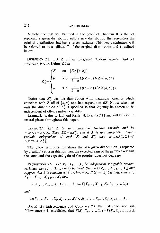
A technique that will be used in the proof of Theorem B is that of replacing a given distribution with a new distribution that resembles the original distribution, but has a larger variance. This new distribution will be referred to as a “dilation” of the original distribution and is defined below.

DEFINITION 2.3. Let Z be an integrable random variable and let - co<a<b<oo. Define Zi as

P on {Z# Ca;bl)

i

b z;=

W.P. &Et@-a)I{ZECa,bl))

a w.p. & E((b - Z) Z{ZE [a, b]}).

Notice that Z”, has the distribution with maximum variance which coincides with Z off of [a, b] and has expectation EZ. Notice also that only the distribution of Z 5: is specified so that Zt may be chosen to be independent of other random variables.

Lemma 2.4 is due to Hill and Kertz [4, Lemma 2.23 and will be used in several places throughout this paper.

LEMMA 2.4. Let Z be any integrable random variable and let -CO <a < b < a~. Then EZ= EZ:, and if X is any integrable random variable independent of both Z and Zt then E(max{X, Z})< E(max{X, Zi>).

The following proposition shows that if a given distribution is replaced by a suitably chosen dilation then the expected gain of the gambler remains the same and the expected gain of the prophet does not decrease.

PROPOSITION 2.5. Let X,, X,, . . . . X, be independent integrable random variables. Let j E ( 1, 2, . . . . n- 1) be fixed. Set v= V(Xj+l, Xj+z, .,.,X,) and suppose that b is constant with v < b < + co. Zf Zj = (X,)! is independent of X 1, . . . . Xjvl, Xj+l, ..,, X, then

VW, 7 **., xj- IT xj, xj+ 1) ...9 Xn) = v/(X1 3 ..-3 Xj- 19 zj, xj+ 13 ...9 xn)

and

Proof. By independence and Corollary 2.2, the first conclusion will follow once it is established that V(Z,, Xi+ I, . . . . X,) = V(Xj, Xi+ 1, . . . . X,).


This follows from easy calculations using Corollary 2.2 and Definition 2.3. That M(Xi, . ..) Xi-1, Xj, Xj+l, . ..y X,)GM(X,, . . . . Xj-1, Zj, X’+i, . . . . X,) follows from repeated application of Lemma 2.4. 1

3. PROOFS OF THEOREMS A AND B

Theorem B can now be used to establish the main result, Theorem A. To simplify expressions, the V, M, and D notation of Section 2 will be used throughout the rest of the paper.

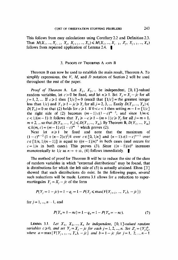
Proof of Theorem A. Let Xi, X,, . . . be independent, [IO, l]-valued random variables, let c > 0 be fixed, and let n > 1. Set Yi = Xj - jc for all j= 1, 2, . . . . If c > 1 then [l/c] = 0 (recall that [l/c] = the greatest integer less than l/c) and Y1 > 1 -jc > Yj for all j= 2, 3, . . . . Easily D( Y,, . . . . Y,,) < D( Y,) = 0 so that (2) holds for c > 1. If 0 <c < 1 then setting m - 1 = [l/c] the right side of (2) becomes (m - 1) c(1 - c)~- ‘, and since l/m < c<l/(m-1) it follows that Y,a--c>l-(m+l)caYjfor allj=m+l, m + 2, . . . so that D( Y,, . . . . . Y,) < D( Yi, . . . . Y,). By Theorem B, D( Y,, . . . . Y,,,) < k(m, c) = (m - 1) c( 1 - c)“-I which proves (2).

Next let n 2 1 be fixed and note that the maximum of (l-~)“-~(l+(n-2)~)*/4 over CE[O, l/n] and (n-l)c(l-CC)“-’ over c E [l/n, l/(n - l)] is equal to ((n - 1)/n)” in both cases (and occurs for c= l/n in both cases). This proves (3). Since ((n- 1)/n)” increases monotonically to l/e as n + + co, (4) follows immediately. 1

The method of proof for Theorem B will be to reduce the size of the class of random variables in which “extremal distributions” may be found, that is distributions for which the left side of (5) is actually attained. Elton [3] showed that such distributions do exist. In the following pages, several such reductions will be made. Lemma 3.1 allows for a reduction to super- martingales Yj = Xj - jc of the form

P(Yj=l-jC)=l-qj=l-P(Yj<maX(V(~.+,,..., Y,), -jC})

for j= 1, . . . . n - 1, and

P(Y,=l-nc)=l-q,=l-P(Y,=-nc). (7)

LEMMA 3.1. Let X,, X2, . . . . X, be independent, [O, 1 ]-valued random variables c 2 0, and set Yj = Xj - jc for each j= 1,2, . . . . n. Set Zj = ( Yj),“, where a = max{ V( Yj+ 1, . . . . Y,), -jc} and b=l-jc for j=l, 2 ,..., n-l

244 MARTIN JONES

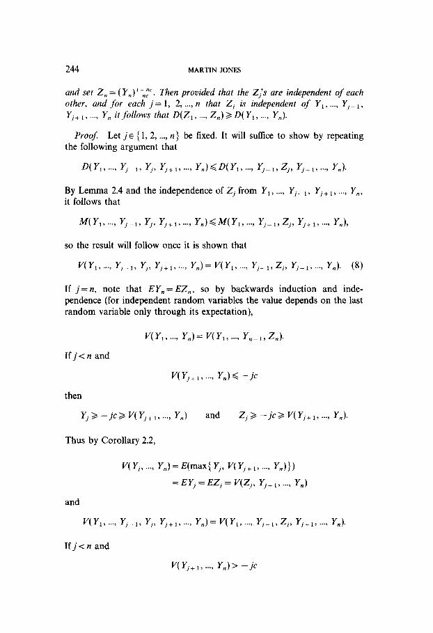
and set Z, = ( Y,,)\J,~?. Then provided that the Zj’s are independent of each other, and for each j= 1, 2, . . . . n that Z, is independent of Y,, . . . . Yj- 1, yj+l, ..,> Y,, it follows that D(ZI, . . . . Z,) 3 D( YI, . . . . Y,,).

Proof: Let jE { 1, 2, . . . . n} be fixed. It will suffice to show by repeating the following argument that

D(y,? ...Y yj-l, Yj, Yj+l, . ..> yn)<D(Y,, .**) Yj-1, Zj, yj+ly ...) Y”).

By Lemma 2.4 and the independence of Zj from Y, , . . . . Yj_ i, Yj+ i, .,., Y,,, it follows that

WY,, ‘.., yj-l, yj, yj+l, ...9 Yn)<M(Y,, ...) yj-,, Zj, Yj+l, ...3 Yn),

so the result will follow once it is shown that

v y, 7 .‘., Yj-1, Yj, yj+l,..., Yn)=v(yl,..., yj-l,zj3 yj+l,..., yH). t8)

If j = n, note that EY, = EZ,, so by backwards induction and independence (for independent random variables the value depends on the last random variable only through its expectation),

V(Y 1, . . . . Y,)= V(Y,, . . . . Y,-1, Z,).

If j<n and

V(yj+~, . . . . Y,)d - jc

then

Yj>-jc>V(Yj+l,..., Y,) and Zj>/-jc2V(Yj+1,..., Y,).

Thus by Corollary 2.2,

V( Yj, . ..) Y,)=E(maX(Yj, v(yj+l, -, Y,)})

= EY, = EZj = V(Zj, Yj+ ,, . . . . Y,,)

and

I/(y 1, ...? Yj- 1, Yj, yj+ 1, ...) Y”) = V( Y,, ...) Yj- 1) Zj, Yj+ 1, .**) Y,).

If j<n and

V(Yj+,,..., Y,)> -jc


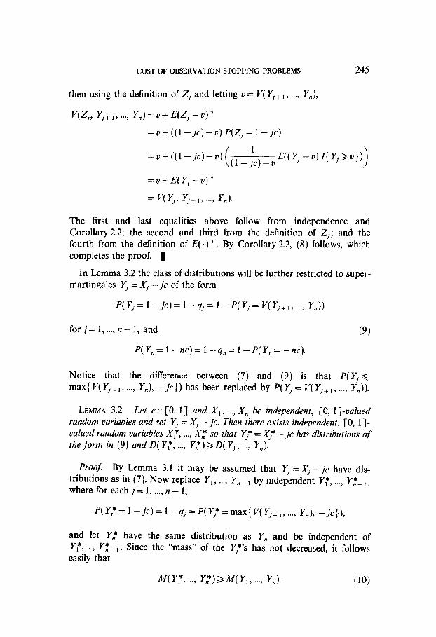
then using the definition of Zj and letting u = V( Yj+ , , . . . . Y,,),

vCzj, yj+ 13 -2 Y,) = II + E(Z, - u) +

=u+((l-jc)-u)P(zj=l-jc)

=u+((l-jc)-u) (

1

(1- jc)-v E((y~-u)z{yj~u})

1

=u+E(Y,-u)+

= V( Yj, Yj+ 1) ..a) Y,).

The first and last equalities above follow from independence and Corollary 2.2; the second and third from the definition of Zj; and the fourth from the definition of E( .) +. By Corollary 2.2, (8) follows, which completes the proof. fl

In Lemma 3.2 the class of distributions will be further restricted to super- martingales Y, = Xj - jc of the form

P(yj=l-jc)=I-qj=l-P(Yi=V(Yj+,,..., Y,))

for j= 1, . . . . n - 1, and

P(Y,=l-nc)=l-qq,=l-P(Y,=-nc).

(9)

Notice that the difference between (7) and (9) is that p( Y, < maxi V( Yj+ i, . . . . Y,), -jc}) has been replaced by P( Yj = V( Y,+ i, . . . . Y,)).

LEMMA 3.2. Let c E [O, 1 ] and X,, . . . . X, be independent, [0, 1 ]-valued random variables and set Yj = Xj - jc. Then there exists independent, [0, I]- ualued random variables X:, . . . . X,* so that Yj* = X3* - jc has distributions of the form in (9) and D(Y:, . . . . Y,*) 3 D( Y,, . . . . Y,).

Proof By Lemma 3.1 it may be assumed that Yj = Xj - jc have distributions as in (7). Now replace Y,, . . . . Y,- i by independent Y:, . . . . YX- L, where for each j= 1, . . . . n - 1,

P(Yj*=l-jc)=l-qj=P(Y:=max{V(Yjtl,..., Y,), -jc]),

and let Y,* have the same distribution as Y, and be independent of Yf, . ..) r;-, . easily that

Since the “mass” of the Y;C’s has not decreased, it follows

M( Y:, .-., Y,*) 2 M( Y1 ) . ..) Y,). (10)

246 MARTIN JONES

Also, an easy calculation of V( Y:, . . . . Y,*) using Corollary 2.2 and noting that YF, . . . . Y,* is a supermartingale yields that V( Yj*, . . . . Y,*) = V( Y,, . ..) Y,) for all j= 1, . . . . II and, in particular,

V( rp, . ..) Y,*) = V( Y1) . . . . Y,). (11)

Now if V( Yj + I, . . . . Y,) = max{ V( Yj+ 1, . . . . Y,), - jc} for each j = 1, . . . . n - 1 then the lemma is proved. Otherwise it must be shown that by decreasing some of the qj’s it is possible to obtain V( Yj+ 1, . . . . Y,) = maxi V( Yj+ 1, . . . . Y,), -jc} and still have (10) and (11) satisfied. Since Y: is a supermartingale V( Yj*, . . . . Y,*) = EY,* for all j= 1, . . . . n and if EY,*, r < -jc for some j = 1, . . . . n - 1 then q,+ r > 0. This follows from the fact that for c~[O,l], if qj+l=O then EYF+,=l-(j+l)c>-jc. Thus qj+ , may be reduced until EYi*, I = -jc. Check that (10) and (11) still hold. 1

Lemma 3.3 is a slight generalization of a result from Hill and Kertz [4] ((2) in Lemma 3.1) to general integrable random variables, from which it follows that for any extremal distribution, X, may be assumed to be constant.

LEMMA 3.3. Let Z,, . . . . Z, be independent integrable random variables and let p= V(Zz, . . . . Z,). Then D(p, Z,, . . . . Z,)2D(Z,, Z,, . . . . Z,).

Lemma 3.4 is a maximization result which is non-probabilistic in nature and serves as the main analytic component in the proof of Theorem B.

LEMMA 3.4. Given a a positive constant and 0 < qi 6 1 for i = 2, 3, . . . . n then the maximum of the function f: R”- ’ -+ R given by f (q2, q3, . . . . q,,) = a n;=, qj subject to the constraints

qn<l-c,

4j(qj+1(..'(4n-1(4n+C)+C)'.')+C)~l-C, for j = n - 1, . . . . 3,

42(4~(.-.(4n-l(qn+C)+C)...)+C)=l-C-~ (12)

where CE (0, 1) and r] E [0, l-S], is attained with q2 = 1 -c-q and q3 = q4 = . . = q” = 1 - c. Moreover, f (1 - c - q, 1 - c, . . . . 1 - c) = a(l-c-q)(1-c)“-2.

Proof: It is first shown that if (q:, q:, . . . . q,*) is a solution to the above constrained maximization problem then q,* = 1 -c. Suppose by way of


contradiction that q,* < 1 -c, and choose 0 < 8 < 1 -c-q;. Let $, = qz+8 and

$ n 1

= 4n*- 1(4n* + cl = 4n*- 1(4n* + c) _ ti,+c q,*+e+c.

Note that $,- l(+n + c) = qz- l(qz + c) so that the constraints in (14) are all satisfied when qx- 1 and qX are replaced by $,-, and $,, respectively. Check also that tin- 1 and +, are in the interval [O, 11. Now

= s,*- ,(d(qn* + 0 + c) + 4 q,+o+c

= sx- 1 qn*(d + 8 + c) + ceq,*- 1 q,*+e+c

=qn*-14n*+ ceq,*- 1 q,*+e+c > 4n*- 14:.

The last inequality will be strict since 8 > 0, c > 0 and it may be assumed that qz- I z=- 0 (since otherwise f = 0). Therefore, f(q:, q:, . . . . qz-*, t,b,- 1,

$,)>f(q2*, q:, .**3 qz), contradicting the optimality of the q*'s. Thus qn*=l-c.

Next suppose that for some 0 <k < n - 3 it has been shown that qtpk = 4:-k+,= ..* = q,* = 1 - c. It will be shown that qzek+, = 1 - c. Under the assumption that qz- k = qz- k + 1 = . . . = qz = 1 -c the constraints in (12) become

qn- k+l<l-C;

s”-k-i(4n-k-i+l(...(4”-k-2(q”-k+,+C)+C)...)+C)

<l--c, for j=2,...,n-k-3, (13) q2(q3(‘.‘(qn-k-2(qn-k-1+C)+C)...)+C=1-C-fl.

Repeating the previous argument under the assumption that q:- k + 1 < 1 - c

shows that f(qz*,qL.yqL+-2, l-~,...,l--)>f(q2*,q:,~~qn*-~-~, 1 - c, . ..) 1 - c) and thus qzpk- 1 = 1 - c. Therefore, by induction, q: = q4*= ,.. = q,* k 1 - c. Substituting 1 - c into (13) for q3, .,., qn yields q2 = 1 - c - q. Finally, direct evaluation gives

f(1 -c--q 1 -c, . ..) 1 -c)=a(l -c-?/)(1 -c)“-2,

as desired. 1

248 MARTIN JONES

The tools to prove Theorem B have now been developed.

Proof of Theorem B. Define for each n = 1, 2, . . . and each c > 0, fi(n, c) := sup{&max l<i<n(xj-jc)) - SUPteT,E(Xt-tc): WI5 ...9 Xn)E C(n)). It will be shown by induction on n that &n, c) = k(n, c) for all n = 1, 2, . . . and all c 3 0. The conclusion is trivial for n = 1 and all c > 0, so suppose that the conclusion holds for n = 1, . . . . m - 1, and all c 2 0. Let tx; 3 . ..> X,) be in C(m), c > 0 and set Yj =X, - jc for j= 1, . . . . m. If c b l/(m - 1) then it follows that D( Y,, Yz, . . . . Y,,,) f D( Y, , Yz, . . . . Y,,- i), so that f(m, c) d R(m - 1, c). Since easily f(m, c) 2 k(m - 1, c), it follows from the inductive hypothesis that &m, c) = k(m - 1, c).

For the remainder of the proof assume that c E [O, l/(m - 1 )] and let (Xl 3 ..., X,,,) E C(m) be such that D(X, - c, . . . . X, - mc) = &m, c) (recall that by Elton [3] such distributions do exist). Again letting Yj = Xj -jc for j= 1, . . . . m, it follows from Lemma 3.2 that Y,, . . . . Y,,, may be assumed to have distributions as in (9). By Lemma 3.3 it may be further assumed that Y, = V( Y,, . . . . Y,). Now if V( Y,, . . . . Y,) > 1 - mc then

my,, y*,-9 Y,)<D(Y,, Y2,.-, Y,-1) < &(m - 1, c) = k(m - 1, c) < k(m, c),

where the equality follows from the inductive hypothesis. Therefore it will be assumed that V( Y,, . . . . Y,) d 1 - mc.

Now using the optimal stopping time t* = (min j: Yj < V( Yj+ i, . . . . Y,) if such j exists and equals n otherwise}, V( Y,, . . . . Y,) can be calculated and

V( y, 9 .**, Y,)=(l-2c)(l-q,)+(l-3c)q,(l-q,)+ ...

+(I -(n- l)c)q,...q,-2(l -CL-1)

+(l-q,-nc)q,...q,. (14)

Also, letting y = V( Y,, . . . . Y,) and noting that y > V( Yj+ ,, . . . . Y,) for all j= 2, 3, . . . . n, it follows that

M( Y, 3 . . . . Y,) = (1 - 2c)( 1 - q2) + (1 - 3c) q2( 1 - q3) + . ‘.

+ (1 -nc)q,... 4n-l(l-qn)+Y fi 4i. (15) i=2

Subtracting (14) from (15) yields D( Yi, . . . . Y,) = (y + nc) nl=, qi. There- fore

D( y, 7 -.*, YJ=(.Y+nc) fi qi, i=2


where Y,, . . . . Y,, satisfy the following constraints,

v( yj, ..a) Y,)> -(j- l)c,

for j = 3, . . . . n, and

V( y,, .-., Y,)=ye[-c, l-nc].

Writing the constraints in terms of the qi)s, the following form can be obtained:

qn<l-c

qn-l(qn+c)G 1 --c

(16)

q3(q4( . . . (qn- ,(%I + c) + c) . . . ) < 1 - c 92(q3(...(4n-1(qn+C)+C)...)+C)=1-C-(y+C).

Suppressing the role of the random variables Y, , . . . . Y, and writing D for D( y, 7 --*, Y,), the objective is now to maximize

D=(y+nc) fi qi i=2

(17)

as a function of the 4;s subject to the’ constraints in (16) and the earlier assumption that CE [0, l&z-- l)]. The claim is that the form of the solution to this maximization problem is given by

D=(y+nc)(l-c)“-2(1--c-y). (18)

To see this, note first that if c =0 then the last constraint in (16) reads n;= 2 qi = 1 - y which when substituted into (17) yields D = y( 1 - JJ). This agrees with (18) in the case that c=O. If CE (0, l/(n- l)] then apply Lemma 3.4 with a = y + nc and q = y + c, which yields an extremal distribution for Y,, . . . . Y, with q2=1-2c-y and q3=q4= ... =qn=l-c. Substitution of these 4;s into (17) yields (18), which proves the claim.

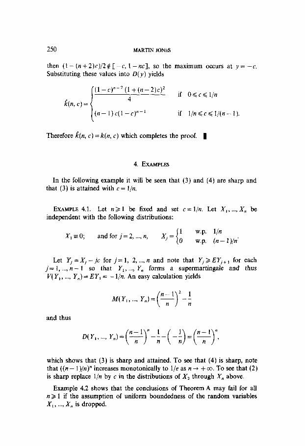
Now for c E [O, l/(n- l)] fixed, D(y) = D = (y + nc)(l - c)~-~ (1 - 2c - JJ) is maximized over y E C-c, 1 - nc]. It follows from D’(y)=(1-~)“-~(1-2y-(n+2)c) that D'(y)=0 if and only if y = (1 - (n + 2)c)/2. If c E CO, l/n] then, since D(y) is negative quadratic in y, there will be a maximum at y = (1 - (n + 2)c)/2. If c E (l/n, l/(n - l)]

250 MARTIN JONES

then (1 - (n + 2)c)/2 $ C-c, 1 -nc], so the maximum occurs at y = -c. Substituting these values into D(y) yields

1 (l-c)n-*(l+(n-2)c)2

4 if O<c< l/n

f(n, c) = (n-l)c(l-CC)“-’ if l/n < c ,< l/(n - 1).

Therefore &(n, c) = k(n, c) which completes the proof. 1

4. EXAMPLES

In the following example it will be seen that (3) and (4) are sharp and that (3) is attained with c= l/n.

EXAMPLE 4.1. Let n > 1 be fixed and set c = l/n. Let X,, . . . . X, be independent with the following distributions:

X,=00; and for j = 2, . . . . n, xj = 1 w.p. I/n 0 w.p. (n - 1 )/n’

Let Yj = Xi - jc for j= 1, 2, . . . . n and note that Yj > EY,, 1 for each j= 1, . . . . n - 1 so that Y,, . . . . Y, forms a supermartingale and thus V( y, , .**, Y,) = EY, = - l/n. An easy calculation yields

n-l* 1 M(Yl, .,.) Y,)= - --

( ) n n

and thus

which shows that (3) is sharp and attained. To see that (4) is sharp, note that ((n - 1)/n)” increases monotonically to l/e as n + + co. To see that (2) is sharp replace l/n by c in the distributions of X2 through X,, above.

Example 4.2 shows that the conclusions of Theorem A may fail for all n 2 1 if the assumption of uniform boundedness of the random variables x 1, . . . . X, is dropped.

COSTOFOBSERVATIONSTOPPINGPROBLEMS 251

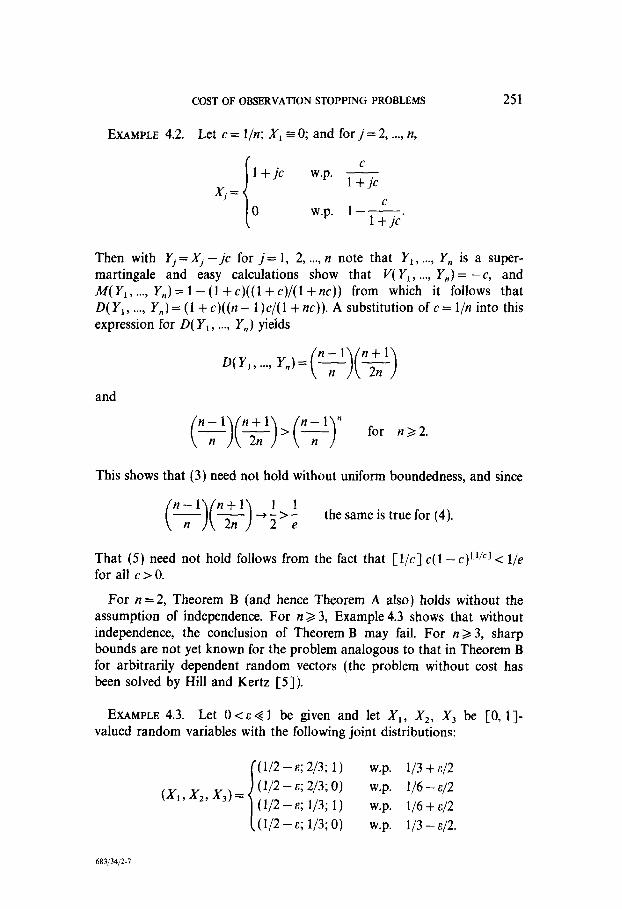
EXAMPLE 4.2. Let c = l/n; XI = 0; and for j = 2, . . . . n,

1 l+jc c

w.p. - Xi=

l+jc

0 w.p. 1 -A l+jc’

Then with Yj = Xj - jc for j= 1, 2, . . . . n note that Y,, . . . . Y, is a supermartingale and easy calculations show that V( Y,, . . . . Y,) = -c, and MY,, ***, Y,,) = 1 - (1 + c)((l + c)/(l + nc)) from which it follows that D( y,, . . . . Y,) = (1 + c)((n - l)c/( 1 + nc)). A substitution of c = l/n into this expression for D( Y,, . . . . Y,,) yields

w y1, . ..> Y”)+yfg)

and

(+)(T)>(y)” for n>2.

This shows that (3) need not hold without uniform boundedness, and since

(9)(G)+:>: thesameistruefor(4).

That (5) need not hold follows from the fact that [l/c] c(1 - c)~“” < l/e for all c > 0.

For n=2, Theorem B (and hence Theorem A also) holds without the assumption of independence. For n> 3, Example 4.3 shows that without independence, the conclusion of Theorem B may fail. For n > 3, sharp bounds are not yet known for the problem analogous to that in Theorem B for arbitrarily dependent random vectors (the problem without cost has been solved by Hill and Kertz [S]).

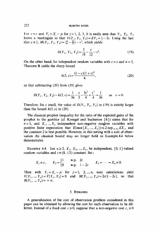
EXAMPLE 4.3. Let 0 <E << 1 be given and let X,, X,, X, be [0, I)- valued random variables with the following joint distributions:

(l/2 - E; 2/3; 1) w.p. l/3 + E/2 (l/2 - E; 2/3; 0)

(x1p *zy*3)= (1/2-c; f/3; 1)

i

w.p. l/6 - &/2 w.p. l/6 + E/2

(l/2 - E; l/3; 0) w.p. l/3 - E/2.

683/34/2-l

252 MARTIN JONES

For c = E and Yj = Xi - j.s for j= 1, 2, 3, it is easily seen that Yi, Y2, Y, forms a martingale so that V( Y,, Y,, Y,) = EY, = 4- 2s. Using the fact that ~61, M(Y,, Y?, Y,)=g-Es-s’, which yields

D(Y,, Y2, Y,)=~+. (19)

On the other hand, for independent random variables with c = E and n = 3, Theorem B yields the sharp bound

q3 7

E)= (1 --EN1 +sj2 4 ’ (20)

so that subtracting (20) from (19) gives

Therefore, for E small, the value of D( Y,, Y2, Y3) in (19) is strictly larger than the bound k(3, E) in (20).

The classical prophet inequality for the ratio of the expected gains of the prophet to the gambler (cf. Krengel and Sucheston [6]) states that for n > 1, and X1, . . . . X, independent non-negative random variables with positive finite expectation that ‘E(max (Xi, . . . . X, 1) < 2 SUP,~ r, EX,, and the constant 2 is best possible. However, in this setting with a cost of observation the classical bound may no longer hold as Example 4.4 below demonstrates.

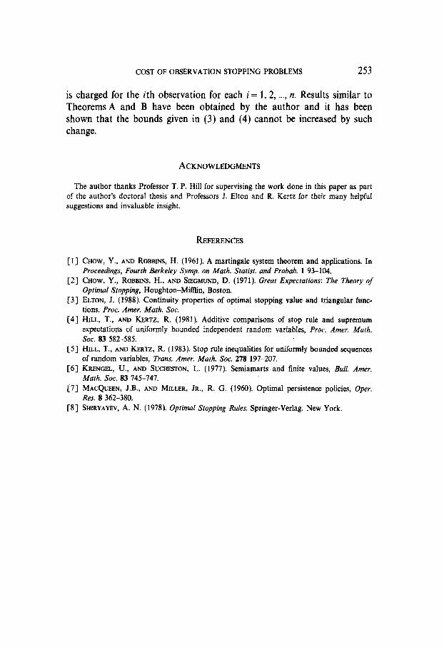
EXAMPLE 4.4. Let n 3 2, Xi, X2, . . . . X,, be independent, [0, I]-valued random variables and c E (0, l/2) constant. Seti

x1=c, x2 = i

1 w.p. 2c 0 w.p. l-2c

x3 = . . . =x, E 0.

Then with Yj = Xj - jc for j = 1, 2, . . . . n, easy calculations yield V(Y Ir . . . . Y,) = V( Y,, Y,) = 0 and M( Y,, . . . . Y,) = 2c(l- 2c), so that R( Y1, . . . . Y,)= +co.

5. REMARKS

A generalization of the cost of observation problem considered in this paper can be obtained by allowing the cost for each observation to be dif- ferent. Instead of a fixed cost c 2 0, suppose that a non-negative cost ci 2 0


is charged for the ith observation for each i= 1,2, . . . . n. Results similar to Theorems A and B have been obtained by the author and it has been shown that the bounds given in (3) and (4) cannot be increased by such change.

ACKNOWLEDGMENTS

The author thanks Professor T. P. Hill for supervising the work done in this paper as part of the author’s doctoral thesis and Professors J. Elton and R. Kertz for their many helpful suggestions and invaluable insight.

REFERENCES

[l] CHOW, Y., AND ROBBINS, H. (1961). A martingale system theorem and applications. In Proceedings, Fourth Berkeley Symp. on Math. Statist. and Probab. 1 93-104.

[Z] CHOW, Y., ROBBINS, H., AND SIEGMUND, D. (1971). Great Expectations: The Theory of Optimal Stopping, Houghton-Mifflin, Boston.

[3 J ELTON, J. (1988). Continuity properties of optimal stopping value and triangular functions. Proc. Amer. Math. Sot.

[4] HILL, T., AND HERTZ, R. (1981). Additive comparisons of stop rule and supremum expectations of uniformly bounded independent random variables, Proc. Amer. Math. sot. a3 582-585.

[S] HILL, T., AND RnaTZ, R. (1983). Stop rule inequalities for uniformly bounded sequences of random variables, Trans. Amer. Math. Sot. 278 197-207.

[6] KRENGEL, U., AND SUCIESTON, L. (1977). Semiamarts and finite values, Bull. Amer. Math. Sot. 83 745-747.

[7] MACQLJEEN, J.B., AND MILLER, JR., R. G. (1960). Optimal persistence policies, Oper. Rex 8 362-380.

[S] SHIRYAYEV, A. N. (1978). Optimal Stopping Rules. Springer-Verlag, New York.

prophet inequalities for cost of observation stopping problems

Documents