Property Tax Incidence on Cropland Cash Rent

Robert Dinterman∗

Ani Katchova†

2019-02-20

Forthcoming: Dinterman, R. and A.L. Katchova. “Property Tax Incidence on Cropland Cash Rent.” Applied

Economic Perspectives and Policy, 2019. https://doi.org/10.1093/aepp/ppz004

Abstract

We estimate the property tax incidence on rented cropland, defined as the extent to which landowners

can increase cash rental rates to shift the tax burden of property tax to renters. Using the Ohio’s Current

Agricultural Use Value (CAUV) Program, we are able to avoid issues where the market value of farmland

determines the property tax as CAUV assesses farmland in Ohio based on a use-value formula with

historical and state-wide prices, yields, and costs of corn, soybeans, and wheat. Our results indicate that

cash rental rates in Ohio from 2008 through 2017 increased between $0.31 to $0.40 for each additional

dollar of property tax levied on cropland in the short run. Further specifications taking into account

lagged effects of property tax indicates a higher incidence of $0.61 higher cash rent for each additional

dollar of property tax, although this is dispersed over a 3 year time period.

Keywords: agricultural land, Current Agricultural Use Value Program, tax incidence, rental rates

JEL Codes: Q14, Q15, Q18

∗The Ohio State University†The Ohio State University

1

Introduction

Almost 40 percent of all farmland in the US is operated by someone other than the landowner according to

the Tenure, Ownership, and Transition of Agricultural Land (TOTAL) survey administered by the United

States Department of Agriculture (USDA) in 2014 (Bigelow, Borchers, and Hubbs 2016). Landowners that

rent their land to other farmers are apt to do so for a multitude of reasons. Broadly speaking, landowners

may operate all or a portion of their land, may have retired from farm operations but continue to own their

land, and others may only hold land because of speculative or investment purposes or may have limited

knowledge of farming operations as approximately 30% of all farmland is owned by non-operators. On the

opposite side of the same coin are the renters of farmland – with only 10% of all farmland being operated by

a farmer who does not own any land. Farmers that rent typically operate smaller farm businesses and are

more likely to be younger or beginning farmers (Mishra, Wilson, and Williams 2009).1

One reason farmers may decide to rent land is because they lack access to capital to finance the purchase of

land. These types of renters would represent a disadvantaged group and may need farm policy programs to

aid in land acquisition. Other farmers may seek additional rented land as a way to scale up their current

operation without making a long-term commitment or because land prices do not justify purchasing versus

renting. Another group may find that both owning and renting land is a risk-reducing measure in a farm’s

portfolio to changing land values (Kaplan 1985; Katchova, Sherrick, and Barry 2002). Others, especially young

and beginning farmers, may both purchase and lease farmland to start their businesses and typically double

their land ownership and leasing within a decade to expand their operations (Katchova and Ahearn 2016).

Whatever the reason, renters represent a large segment of the farming population and have heterogeneous

preferences and characteristics which affect their relationship with landowners.

Understanding the relationship between landowners and renters can help shape policies that are intended

to affect production decisions for farmers. If the burden of property tax is fully passed from a landowner

to a renter, then its effects may deter production or change the riskiness of the planting decisions for the1While most of farmland that is rented goes to larger farms, the typical farmer that rents land differs because larger farms

are apt to rent larger amounts.

2

renter. As an example of the relationship between production practices and cash rents, Allen and Borchers

(2016) find that the increased prevalence of cash rent contracts, as opposed to crop share rental contracts,

has been the result of no-till cultivation practices which have reduced the the ability of a renter to exploit

landowner’s soil. However, if none of the tax is passed onto the renter and is fully paid by the landowner, then

taxing of agricultural land would be decoupled from the farming decisions of the operators. Increasing tax

on agricultural land would deter agricultural related investment on the land, shift ownership more towards

operators, and suppress land values. The focus of our paper is to leverage knowledge of Ohio’s property tax

program on farmland to estimate the degree to which property tax increases lead to higher cash rents.

Public displeasure of increasing farmland taxes in Ohio began around 2010 where the Norwalk Reflector ran

an article indicating that farmers across the county were both angered and confused with their tax bill after

meeting with the Ohio Farm Bureau (Seitz 2010). The reason for the revision in 2006 stemmed from concerns

surrounding school funding sources in counties where residential taxpayers were paying a substantially larger

share compared to farmers – which disproportionately affected rural counties where more agricultural land is

located (Sutherly 2006).2 The revision resulted in an increase in the property tax bill for Ohio farmers due to

changes in the valuation formula and because of rising crop prices and declining interest rates – which are

the components in the formula. Across the largest newspapers in the Ohio, there were multiple instances

of farmers writing letters to editors to try and address the issue of rising taxes on farmland of which the

Springfield News-Sun interviewed farmland owners in September 2010 to address how farm leases have been

amended in response to increased property taxes (Writer 2010). In 2014, The Columbus Dispatch ran a story

highlighting the rising CAUV values with an interview of Bill Cox – an 81 year old farmer who received an

increase in his tax bill on 105 acres of land from $2,446 the previous three years to $5,412 as his county

received a reappraisal. Bill summed up a large portion of Ohio farmer’s sentiments towards the rising property

taxes with his thoughts: “The money we get for our crops this year pays for our taxes next year; If they’ve

got a formula, they’ve probably got some third-grader working on it” (Narciso 2014). The fever pitch of2In an interview in November 26, 2006, the Ohio Farm Bureau Federation predicted that CAUV values could as much as

double in a couple of years but would still be less than the value assigned for a decade ago (assuredly in real terms). The averagevalue in 2006 tax year was $177 per acre which did not more than double until 2011 with $700 per acre on average. However,the high prior to 2005 in real 2016 dollars was 1999 at around $360 per acre. Since 2009, there has not been a single year below$504 per acre in real 2016 dollars for CAUV values.

3

farmer complaints ended in 2017 when legislation was passed to combat issues with the capitalization rate

that will reduce CAUV values in the six following years through a phase-in period.

Existing literature of property tax incidence on agricultural land has mostly dealt with the value of the

agricultural land with both theory and empirics indicating that increases in property tax negatively affect

the value of agricultural land. Pasour Jr (1975) evaluates the per acre value of farm real estate due to a

change in the effective property tax rate with a cross section of states in 1969. An increase in the effective

tax rate of one mill ($1 per $1,000 of assessed value) results in a decrease of $6.37 per acre in farm real estate

price. Chicoine, Sonka, and Doty (1982) provides a simulation of the Ohio use-value assessment program in

1980 and estimate that the distributional effects of use-value assessments are to immediately increase the

land value and improve the landowner’s equity positions. John E Anderson and Bunch (1989) evaluate the

implementation of use-value assessment to show an immediate effect of increasing farmland values through

the channel of reducing the tax burden. The literature is consistent in its findings that decreases in property

tax increase farmland value and there is shifting of the tax burdens due to use-value assessment programs.

However, the literature has yet to address the landowner-operator relationship and how cash rents may be

affected by changes in property taxes.

There is another substantial body of research which addresses the incidence rate of agricultural policies

between landowner and land operator as it relates to who effectively captures various agricultural subsidies.

This literature has focused on farm rental rates as the main mechanism for landowners to extract agricultural

subsidies from farm operators and finds that landowners capture subsidies from renters estimates ranging

from as low as $0.13 to upwards of $0.60 per dollar of subsidies going to landowners (Alston 2010). Roberts,

Kirwan, and Hopkins (2003) finds an incidence of government payments on land rents between $0.34 and

$0.41 for each government payment dollar using farm level data from the 1997 Census of Agriculture. In a

follow-up by Kirwan (2009) which links the 1992 and 1997 Censuses of Agriculture for repeated farm level

observations, they find a smaller incidence of $0.25 for each additional dollar in government payments. Using

pooled cross-sections of ARMS from 1998 to 2005, Goodwin, Mishra, and Ortalo-Magné (2011) finds an

incidence rate of around $0.32 per dollar of subsidies. Hendricks, Janzen, and Dhuyvetter (2012) estimate the

4

incidence rate using a panel of Kansas farmers from 1990 to 2009 and find that landowners capture $0.12 for

each additional dollar in government subsidies in the short-run and provide a long-run estimate of $0.37 per

dollar. Kirwan and Roberts (2016), using field level data from ARMS Phase 2, find a lower incidence rate as

between $0.20 to $0.28 for each government payment is being captured by the landowner which is a much

lower rate than the $0.42 to $0.49 per dollar from their farm-level analysis of the same data. Within the

government program incidence rate literature, the level of dis-aggregation for the data and ability to track

observations over longer periods of time appear to indicate smaller incidence rates.

To our knowledge, this is the first study to address how property taxes on agricultural land are passed from

landowners onto renters in the form of higher cash rents and further bridges a gap in the incidence rate

literature as it relates to taxes instead of subsidies. Our study analyzes the property tax incidence rate of

shifting the property tax burden from landowners to renters in the form of higher cash rents using changes in

the Current Agricultural Use Value Program (CAUV) of Ohio which are exogenous to the rental market.

The program provides differential property tax treatment for agricultural land – based solely on the soil type

of the land – by valuing agricultural land at its use-value for assessment purposes as opposed to its market

value that all other types of property in Ohio are assessed at. As farmland property taxes are independent of

market forces, as further explained in CAUV Overview section, endogeneity concerns between property taxes

and cash rents in Ohio are largely alleviated.

Our study’s objective is to provide an estimate for the tax incidence rate – the increase in the cash rental rate

per acre of farmland due to a change in the property tax paid per acre of farmland. Ohio provides a unique

policy for taxing farmland that allows for estimating tax incidence due to its differential tax treatment of

agricultural land that explicitly does not depend on cash rents within the county or state, whereas surrounding

states like Indiana uses data on cash rents to form their assessed value of farmland (DeBoer 2008). Our

estimation procedure involves panel data estimation of county level cash rents on property tax which allows

us to control for factors affecting both. Our results indicate an additional $1 of property tax levied on an

acre of rented land leads to a $0.31 to $0.40 increase in the cash rental rate. These estimates control for

agricultural factors, temporal trends, and county characteristics across Ohio that are related to both the cash

5

rental rate and property tax payments, although longer run estimates indicate a higher incidence ($0.61) as

land owners appear to increase cash rents over a longer period of time to recoup increased property taxes.

These estimates indicate a higher rate of incidence for landowners than what previous studies have established

for incidence rates of landowners capturing subsidy payments, part of which may be due to the simplicity

and transparency of a property tax versus government payments.

The paper proceeds by first introducing CAUV and its changes in both calculation and values over the years

of interest. Next, conceptual issues for estimating tax incidence are addressed with emphasis on how CAUV

mitigates these concerns due to its design in the CAUV Overview section. Then, the regression framework is

described in Conceptual Issues section followed by a description of the data in the Data section. Results are

presented and interpreted followed by a discussion between shorter and longer run effects of the property

tax changes in the Results section. Finally, the paper concludes with a discussion on the policy implications

which can be inferred from the results along with avenues of future research in the Conclusions section.

CAUV Overview

In 1974, Ohio enacted the Current Agricultural Use Value Program (CAUV) as a tax incentive for farmers to

continue agricultural production on their land instead of developing it due to urbanization pressure. CAUV

provides an appraisal method for valuing agricultural land by using only agricultural inputs rather than the

market value of land (Jeffers and Libby 1999). Throughout the 1970s, other states adopted similar programs

of differential appraisal methods of agricultural land in the same vein and, as of 2014, all 50 states within

the US provide some sort of differential tax treatment of agricultural land to tax at less than market value

(Sherrick and Kuethe 2014). While each state has its impetus for enacting preferential tax treatment and its

particular calculation, the intent behind differential taxation is generally understood as applying a net present

valuation of agricultural production that is not tied to potential urbanization development pressures (John E

Anderson 2012). Ohio is no different and has developed its own calculation method that depends on soil type,

crop yields/prices/rotation, operational costs, and capitalization rate. The basic premise has been in place

since the late 1970s although the program has become more sophisticated and received substantial updates in

6

1984, 2006, 2015, and most recently in 2017 that have affected the calculation of CAUV (Shaudys 1980).

The Ohio Department of Taxation (ODT) determines the use-value for agricultural land based on recommen-

dations from the Ohio Farm Bureau who periodically set the formula which uses values related to Ohio’s

agricultural economy. The calculation of CAUV values involves the past 5 to 10 years worth of state-level

data on yields, prices, costs, and interest rates in deriving a property’s taxable value. CAUV values inherently

reflect past market conditions and do not account for the net present value of future market returns to land

like a market assessment would. CAUV calculations are also independent of actual planting decisions of

farmers, which implies a farmer growing corn and a farmer growing soybeans with identical soil types would

have the same CAUV value even if the expected revenues of corn and soybean production substantially differ.3

Effectively, every soil type throughout Ohio is assigned a CAUV value each year that depends on state-wide

average costs/revenues for corn, soybeans, and wheat over the previous 7 to 10 years. For a given parcel, its

total CAUV value will depend on the acreage of each soil type within the parcel. Soil types that have higher

productive capacity – based on 1984 values from the most recent comprehensive soil survey in the state – will

have higher CAUV values than those with lower productive capacity.4 Zobeck, Gerken, and Powell (1983)

provides a comprehensive soil productivity index for every soil type in Ohio based upon relative yields of

corn, soybeans, wheat, oats, and hay across the state of Ohio. The index ranges from 0 to 100 and provides a

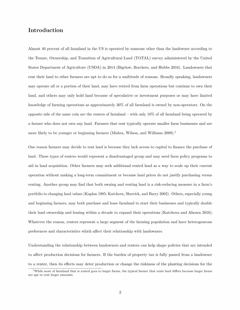
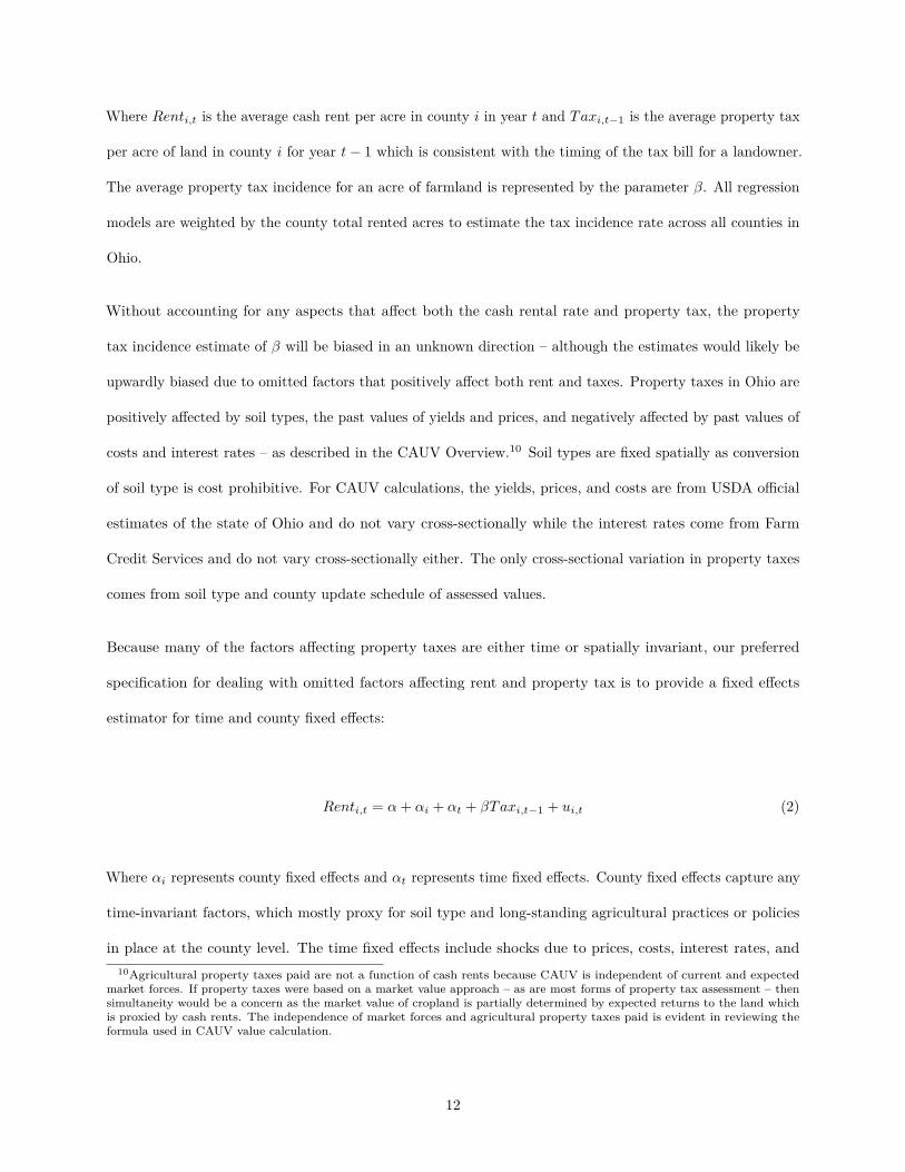
barometer for how productive soil types across the state are. Figure 1 places soil types in bins according to

their productivity index and plots the average CAUV value since 1991 to provide a range of CAUV values.

ODT provides an additional mandate for a minimum CAUV value. Prior to 2009, this was $100 but the value

subsequently rose to $170, $200, $300, and finally $350 in 2012. More detail on the calculation of CAUV

values can be found in the appendix.

The only factor that varies spatially in CAUV calculations is the soil types across Ohio and the reappraisal

schedule for a county. Soil types do not change over time, therefore much of the effect of soil type on

property taxes is fixed cross-sectionally. To the degree that land enrolled or taken out of CAUV changes the3CAUV is also independent of the agricultural activity the land is used for – for example, livestock and aquatics both receive

the preferential tax treatment from CAUV and their property tax is based off of soil type of the land.4However, some soil types are relatively more productive with respect to one crop than the others; there is not a monotonic

relationship across soil types ranking of CAUV values.

7

composition of soil types for a county, this is not an empirical concern. Since 1990, total acreage enrolled in

CAUV has been fairly stable although there have been some small declines in enrolled CAUV acreage for

counties under urbanization pressure as farmland is converted to residential or commercial purposes.5 For

agricultural land to be eligible for CAUV, it must either be at least 10 acres devoted exclusively to commercial

agricultural use or be able to produce more than $2,500 in average gross income. The overwhelming majority

of farmland in Ohio is enrolled in CAUV and it is likely the case that more land is enrolled in CAUV than

farmable according to Prindle (2014).

For both agricultural and residential properties, a full property re-assessment occurs once every six years

with an adjustment occurring three years prior to the full re-assessment based upon sales data of similar

properties and provides for a market-based valuation procedure. Adjustment schedules vary by county while

each county has been on the same schedule since the 1970s.6 The adjustment is a percentage change based

on similar properties sales transaction data in that county. CAUV values adjust once every three years but

always in conjunction with a re-assessment or adjustment for a county. After CAUV values change for a

county, landowners know their CAUV values for the current and following two years but the CAUV value is

not known until after the taxable year because of the backwards nature of CAUV calculations.7 Tax bills for

a given calendar year are fully paid by the landowner around the middle of the next calendar year.

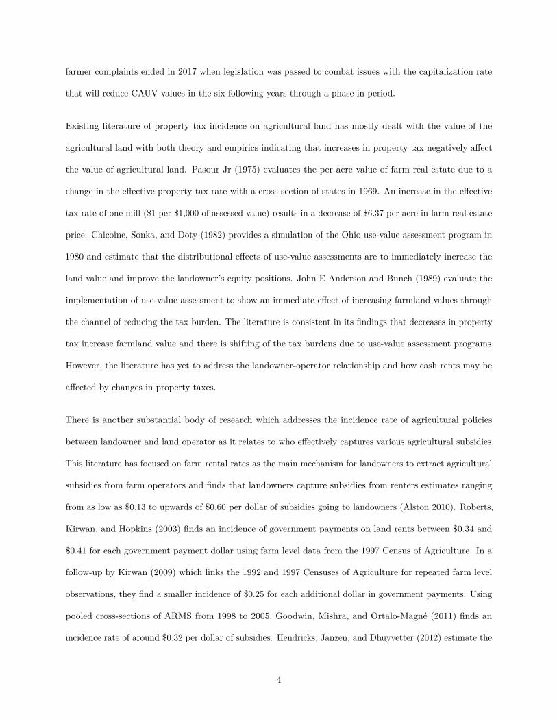
In spite of the trend of increasing agricultural land values in the state of Ohio since the mid-1980s, its

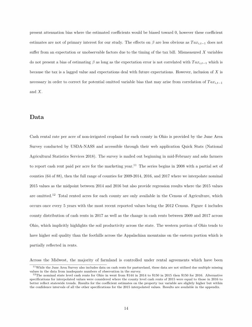
cropland cash rental rates in real terms stagnated from 1994 until 2005. Figure 2 displays a time series of the

Ohio’s average rental price for an acre of cropland and the average amount of property tax paid per acre

of agricultural land in 2016 dollars. In 1994, property tax represented 8.50% of the cash rental rate and

increased to 20.1% in 2017 throughout this time, representing a substantial increase in property taxes relative

to cash rental rate. ODT announced a revision to their valuation procedure of agricultural land for tax

purposes in 2005 which would first apply to the counties receiving updates to the property tax assessments in5When a landowner decides to unenroll from CAUV for this purpose, they must pay a recoupment penalty that is equal to

the CAUV tax savings for the previous 3 tax years – i.e. the difference between market value and CAUV. Prindle (2014) notesthat it is not clear if ODT has maintained consistent data recording of recoupment penalties in order to assess the extent towhich land has been taken out of CAUV.

6In 2017, half of the counties received updated CAUV values while in both 2016 and 2015 a quarter of the counties receivedupdated CAUV values.

7The 2014 TOTAL Survey reports that almost 74% of rental agreements are up for renewal annually, less than 4% arebiannually, and less than 10% are on a 3 year schedule. The remainder are on a renewal term of 4 years or greater.

8

the 2006 tax year (by 2008 tax year, all counties had received CAUV values from the updated formula).

John Edwin Anderson and England (2014) provides an overview of various state programs for preferential

taxation of farmland across the United States. Overall, there are three main forms of preferential tax

treatment: 1) a percentage reduction from fair market value (e.g., Georgia, Minnesota, and Mississippi), 2)

capitalization of average cash rental rate (e.g., California, Tennessee, and Virginia), and 3) capitalization of

net income approach (e.g., Illinois, Iowa, and Pennsylvania) although some states combine the capitalization

of average cash rental rate and net income approach (e.g., Kentucky, Indiana, and North Carolina). The first

two forms of preferential tax treatment pose obvious endogeneity problems as property tax is determined

from cash rental rates as property values inherently include the net present value of expected future income

from the land (i.e. rents).8 Ohio exclusively uses the third method, the dominant form across the United

States, at the soil type level. Ohio’s formula uses state-level values for costs, prices, and yields which provides

a substantial amount of variation across farms but not so fine-scaled so as to completely proxy local cash

rents. States surrounding Ohio typically do not have as fine scaled of valuation procedure at the soil level

while also not completely proxying local cash rents. Illinois provides valuation at the soil type level but uses

county yields as an adjustment. Indiana groups soil types together in their net income approach but this

is averaged with surveyed cash rents for a county. In Iowa, the net income valuation is consistent across a

county by using county level data on yields. Ohio eschews much of the endogeneity concerns in estimating a

relationship between cash rents and property taxes but there are still some concerns which we elaborate on in

the next section.

Conceptual Issues

The taxable value of property in Ohio is 35% of its assessed value for all property except agricultural land,

which uses CAUV in place of assessed value. The property tax due is based on the taxable value as well

as the millage rate for the taxing districts that the land is located in. Counties, municipalities, and school8All states use at least one year lagged values of data, but the typical time frame is the past 10-years worth of data. No state

uses any forward looking measure of property values, expected cash rents, or future costs/revenues.

9

districts all have varying degrees of taxation powers within Ohio which creates an element of spatial variation

for property tax payments. Millage rates will vary based on locations and how many taxing districts are

present in an area. Millage rates for individual counties are fairly stable over time but there is a substantial

amount of variation in millage rates across Ohio mostly based on the population density of a county as they

are typically higher near urban centers which typically demand more services from governments.

The predetermined and backward looking nature of changes in assessed values is the main crux for identification

of tax incidence for renters. Although landowners and renters can anticipate when they will receive new

CAUV values, they are unlikely to accurately anticipate what the actual change in the CAUV value will

be based on the complexity of the formula and the legislative uncertainty at the time which led to various

changes in the formula. This layer of uncertainty and its delayed payment helps in identifying tax incidence

on renters.

Farmland property tax incidence is measured as the additional amount paid by the renter/operator for one

more dollar of property tax levied on the landowner. For an owner who is also the operator, all of the

additional tax is paid by the operator. However, if a landowner rents out their land, they can potentially

raise the rent to offset property tax increases. If the landowner pays 100% of the additional tax, then the tax

incidence for a renter/operator is 0 and would represent a situation where land supply is perfectly inelastic or

demand is perfectly elastic. Vice-versa, a renter pays 100% of the additional tax when demand for rented

cropland is perfectly inelastic or supply is perfectly elastic.

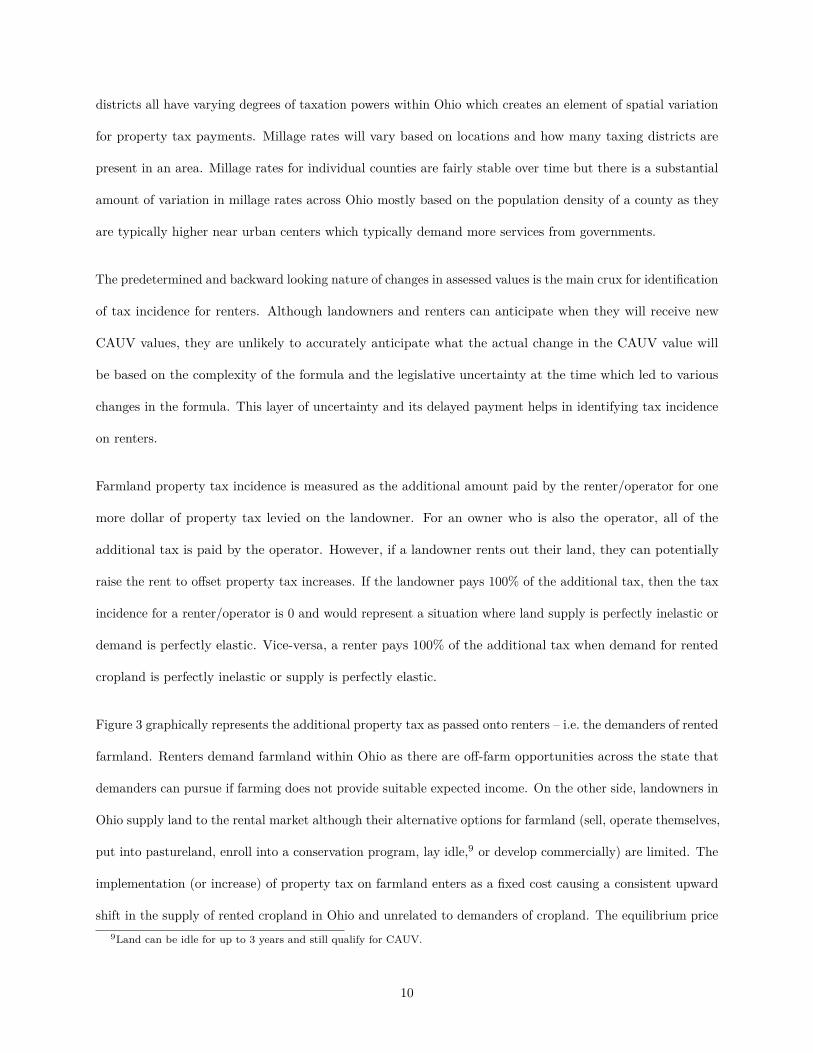
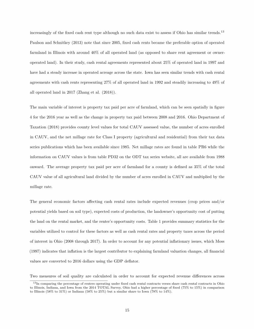
Figure 3 graphically represents the additional property tax as passed onto renters – i.e. the demanders of rented

farmland. Renters demand farmland within Ohio as there are off-farm opportunities across the state that

demanders can pursue if farming does not provide suitable expected income. On the other side, landowners in

Ohio supply land to the rental market although their alternative options for farmland (sell, operate themselves,

put into pastureland, enroll into a conservation program, lay idle,9 or develop commercially) are limited. The

implementation (or increase) of property tax on farmland enters as a fixed cost causing a consistent upward

shift in the supply of rented cropland in Ohio and unrelated to demanders of cropland. The equilibrium price9Land can be idle for up to 3 years and still qualify for CAUV.

10

in the rental market rises and lends to a shared burden between the renters (the dotted-shaded region in

figure 3) versus the owners (the non-dotted shaded region).

The relative elasticities of the demand and supply of farmland in the rental market will dictate the pass-

through rate – i.e. how much of the additional dollar of property tax on farmland can be passed onto renters

in the form of higher cash rents. Renters comprise the set of demanders in the market and the relative

elasticity of demand will be directly related to the off-farm activities that a renter can undertake in order to

reduce their proportion of the property tax paid. On the other hand, relatively limited off-farm activities

that renters can undertake will lead to more inelastic demand and thus push up the proportion of property

tax paid by renters. Similarly, on the supply side of the market, landowners with relatively more options

for their land use would result in a more elastic supply of farmland and increase the proportion of property

tax that a renter will pay. Practically, the farmland market in Ohio is relatively inelastic as there is limited

amount of land which has gone into and out of CAUV since the early 1990s – typically 16 million acres are

enrolled in the program each year. However, there is fluctuation in the rental market as Ohio has had 6.75

million acres rented in 1997, 6.47 million acres rented in 2002, 6.33 million acres rented in 2007, and 6.19

million acres rented in 2012. Land leaving the rental market – as opposed to the CAUV program – is the

anticipated mechanism causing the rise in cash rent prices due to the rapid increase in property taxes in

Ohio, however the particular burden that renters bear in each additional tax dollar is the main contribution

of this paper to the literature.

Regression Framework

We start with a naive estimate of cash rental rates against property tax for all counties in Ohio for non-irrigated

cropland – the dominant rental market of farmland in Ohio:

Renti,t = α+ βTaxi,t−1 + ui,t (1)

11

Where Renti,t is the average cash rent per acre in county i in year t and Taxi,t−1 is the average property tax

per acre of land in county i for year t− 1 which is consistent with the timing of the tax bill for a landowner.

The average property tax incidence for an acre of farmland is represented by the parameter β. All regression

models are weighted by the county total rented acres to estimate the tax incidence rate across all counties in

Ohio.

Without accounting for any aspects that affect both the cash rental rate and property tax, the property

tax incidence estimate of β will be biased in an unknown direction – although the estimates would likely be

upwardly biased due to omitted factors that positively affect both rent and taxes. Property taxes in Ohio are

positively affected by soil types, the past values of yields and prices, and negatively affected by past values of

costs and interest rates – as described in the CAUV Overview.10 Soil types are fixed spatially as conversion

of soil type is cost prohibitive. For CAUV calculations, the yields, prices, and costs are from USDA official

estimates of the state of Ohio and do not vary cross-sectionally while the interest rates come from Farm

Credit Services and do not vary cross-sectionally either. The only cross-sectional variation in property taxes

comes from soil type and county update schedule of assessed values.

Because many of the factors affecting property taxes are either time or spatially invariant, our preferred

specification for dealing with omitted factors affecting rent and property tax is to provide a fixed effects

estimator for time and county fixed effects:

Renti,t = α+ αi + αt + βTaxi,t−1 + ui,t (2)

Where αi represents county fixed effects and αt represents time fixed effects. County fixed effects capture any

time-invariant factors, which mostly proxy for soil type and long-standing agricultural practices or policies

in place at the county level. The time fixed effects include shocks due to prices, costs, interest rates, and10Agricultural property taxes paid are not a function of cash rents because CAUV is independent of current and expected

market forces. If property taxes were based on a market value approach – as are most forms of property tax assessment – thensimultaneity would be a concern as the market value of cropland is partially determined by expected returns to the land whichis proxied by cash rents. The independence of market forces and agricultural property taxes paid is evident in reviewing theformula used in CAUV value calculation.

12

weather events.

If there are factors which vary across time and space that affect both cash rental rate and the property tax

paid on farmland, then equation 2 does not provide a consistent estimate of the property tax incidence rate,

β, due to omitted variable bias. However, many of these factors will be captured within the county and time

fixed effects as the variation in CAUV values are either time-invariant (soil type) or cross-sectionally invariant

(prices, yields, costs, and interest rates). While it is clear that counties across Ohio will have variation in their

crop mixture, yields, and prices received that affects cash rental rates at the county level, CAUV calculation

only uses the state level value for these factors. If each county used their own yields/price/costs for corn,

wheat, and soybeans then it would be a concern to control for each of these factors as variation in property

tax would be based on local factors which vary from year to year. However, these factors are captured in

either county or time fixed effects based on the CAUV calculations.

While data on agricultural and economic factors affecting rental rates and property taxes have limitations –

described in the following data section – inclusion of relevant economic factors can be incorporated into the

estimation procedure as a robustness check of estimated property tax incidence and alleviate concerns of

an omitted variable bias. Inclusion of these agricultural and economic factors in a matrix, X, of covariates

provides an equation of the form:

Renti,t = α+ αi + αt + βTaxi,t−1 + γXi,t−1 + ui,t (3)

A concern with including agricultural and economic factors is the timing lag of negotiated rental rates and

these factors. Rental contracts are typically negotiated prior to the planting season based on expectation

of the agricultural and economic factors that farmers will face during harvest when they receive revenues

from their crops. As such, the lagged agricultural and economic values provide a more accurate proxy of the

expectations of what a farmer will receive in harvest as opposed to the observed harvest conditions. These

expectations are unobservable to the econometrician and may pose an errors-in-variables problem if these

unobservable factors are correlated with ui,t. The errors-in-variables problem will affect γ estimates and

13

present attenuation bias where the estimated coefficients would be biased toward 0, however these coefficient

estimates are not of primary interest for our study. The effects on β are less obvious as Taxi,t−1 does not

suffer from an expectation or unobservable factors due to the timing of the tax bill. Mismeasured X variables

do not present a bias of estimating β as long as the expectation error is not correlated with Taxi,t−1 which is

because the tax is a lagged value and expectations deal with future expectations. However, inclusion of X is

necessary in order to correct for potential omitted variable bias that may arise from correlation of Taxi,t−1

and X.

Data

Cash rental rate per acre of non-irrigated cropland for each county in Ohio is provided by the June Area

Survey conducted by USDA-NASS and accessible through their web application Quick Stats (National

Agricultural Statistics Services 2018). The survey is mailed out beginning in mid-February and asks farmers

to report cash rent paid per acre for the marketing year.11 The series begins in 2008 with a partial set of

counties (64 of 88), then the full range of counties for 2009-2014, 2016, and 2017 where we interpolate nominal

2015 values as the midpoint between 2014 and 2016 but also provide regression results where the 2015 values

are omitted.12 Total rented acres for each county are only available in the Census of Agriculture, which

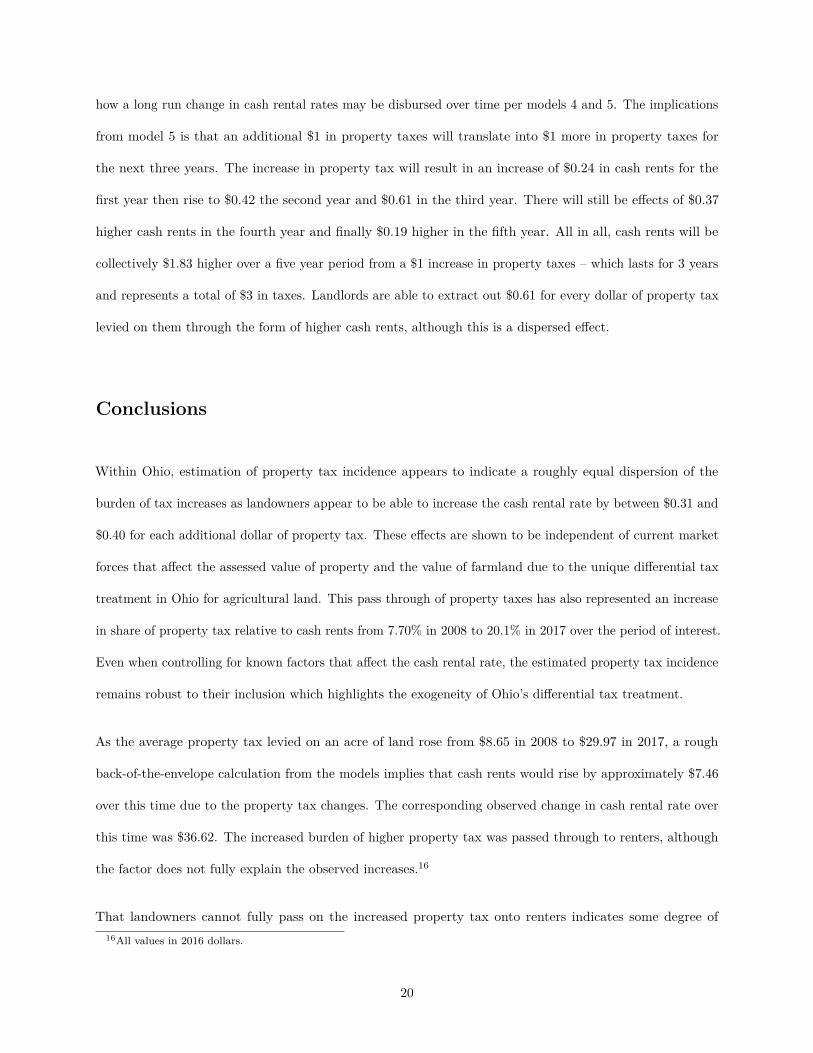
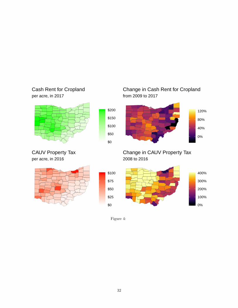
occurs once every 5 years with the most recent reported values being the 2012 Census. Figure 4 includes

county distribution of cash rents in 2017 as well as the change in cash rents between 2009 and 2017 across

Ohio, which implicitly highlights the soil productivity across the state. The western portion of Ohio tends to

have higher soil quality than the foothills across the Appalachian mountains on the eastern portion which is

partially reflected in rents.

Across the Midwest, the majority of farmland is controlled under rental agreements which have been11While the June Area Survey also includes data on cash rents for pastureland, these data are not utilized due multiple missing

values in the data from inadequate numbers of observation in the survey.12The nominal state level cash rents for Ohio in went from $144 in 2014 to $150 in 2015 then $150 for 2016. Alternative

specifications for interpolated values were considered where the county level cash rents of 2015 were equal to those in 2016 tobetter reflect statewide trends. Results for the coefficient estimates on the property tax variable are slightly higher but withinthe confidence intervals of all the other specifications for the 2015 interpolated values. Results are available in the appendix.

14

increasingly of the fixed cash rent type although no such data exist to assess if Ohio has similar trends.13

Paulson and Schnitkey (2013) note that since 2005, fixed cash rents became the preferable option of operated

farmland in Illinois with around 40% of all operated land (as opposed to share rent agreement or owner-

operated land). In their study, cash rental agreements represented about 25% of operated land in 1997 and

have had a steady increase in operated acreage across the state. Iowa has seen similar trends with cash rental

agreements with cash rents representing 27% of all operated land in 1992 and steadily increasing to 49% of

all operated land in 2017 (Zhang et al. (2018)).

The main variable of interest is property tax paid per acre of farmland, which can be seen spatially in figure

4 for the 2016 year as well as the change in property tax paid between 2008 and 2016. Ohio Department of

Taxation (2018) provides county level values for total CAUV assessed value, the number of acres enrolled

in CAUV, and the net millage rate for Class I property (agricultural and residential) from their tax data

series publications which has been available since 1985. Net millage rates are found in table PR6 while the

information on CAUV values is from table PD32 on the ODT tax series website, all are available from 1988

onward. The average property tax paid per acre of farmland for a county is defined as 35% of the total

CAUV value of all agricultural land divided by the number of acres enrolled in CAUV and multiplied by the

millage rate.

The general economic factors affecting cash rental rates include expected revenues (crop prices and/or

potential yields based on soil type), expected costs of production, the landowner’s opportunity cost of putting

the land on the rental market, and the renter’s opportunity costs. Table 1 provides summary statistics for the

variables utilized to control for these factors as well as cash rental rates and property taxes across the period

of interest in Ohio (2008 through 2017). In order to account for any potential inflationary issues, which Moss

(1997) indicates that inflation is the largest contributor to explaining farmland valuation changes, all financial

values are converted to 2016 dollars using the GDP deflator.

Two measures of soil quality are calculated in order to account for expected revenue differences across13In comparing the percentage of renters operating under fixed cash rental contracts verses share cash rental contracts in Ohio

to Illinois, Indiana, and Iowa from the 2014 TOTAL Survey, Ohio had a higher percentage of fixed (75% to 15%) in comparisonto Illinois (58% to 31%) or Indiana (58% to 25%) but a similar share to Iowa (78% to 14%).

15

counties since crop price data across Ohio are only available at the state level.14 USDA’s Natural Resources

Conservation Service (2018) provides data on county level acreage of soil type and each soil type’s National

Commodity Crop Productivity Index (NCCPI) – a productivity index of soil types which ranges from 0 to

100. Both of these variables are time-invariant, which would be captured by county fixed effects and thus not

identified when county fixed effects are present. As an alternative for a variable related to soil quality that

varies over time, an effective productivity index is constructed with knowledge of the total planted acreage

of crops for a county in Ohio. To construct this index, first soil types in a county are arranged in order of

their productivity index from highest to lowest. Then, the county’s total planted acreage for a year is used to

determine all of the soil types in use for a county with the assumption that the highest productivity soils are

first used. And finally, the weighted average of the productivity for soil types in use is calculated with the

acreage of each soil type for the county as the weight. The time variation in planted acreage for counties

creates a time-varying component that can be utilized in a county fixed effects context. When fewer (more)

acres are planted in a county, the lower quality soils drop out of (add to) the weighted average and increase

(decrease) the effective soil productivity index.

Another potential source of revenues includes government payments on cropland, data on which are provided

by the Farm Subsidy Database from Environment Working Group (2018) at the county level from 1995

through 2016. Government programs that made payments from 2008 to 2016 are grouped in terms of

commodity, conservation, crop insurance, and disaster subsidies. The total government payments less

conservation payments are aggregated at the county level and divided by total acreage to provide an estimate

for government payment per acre of agricultural land. Conservation payments – largely from the Conservation

Reserve Program (CRP) – are not included in government payments because land placed in a conservation

program cannot be farmed and thus is not in the rental market. However, CRP has an indirect effect on the

rental market because land in the conservation reserve program is taken off the market for 10 to 15 years at a

time. For land to qualify for CRP, the land must be environmentally sensitive which generally implies land of

lower soil productivity. Enrollment into CRP is optional and induced by payments for removing cropland

from production. Total acreage enrolled affects the available land in the rental market and the total acreage14Historical elevator grain cash bid prices in Ohio are not readily available. It is also not clear how a county level price index

would be calculated from elevator grain prices across the state.

16

is influenced by the payment rate for CRP enrollment – although the CRP payment rate is determined by a

county’s average cash rental rate which would be endogenous to the cash rental rates. Therefore, acreage

enrolled in CRP divided by total farmable acreage in a county is included because it affects both cash rental

rates and average CAUV value in a county.

In addition to CRP and government payments, another concern for a potential variable related to cash rents

and CAUV is the development of shale gas and other mineral rights particularly in the eastern portion of

Ohio. While mineral rights do not directly affect cash rental rates and cannot be included within the CAUV

program due to mineral rights not fitting the criteria of commercial agriculture, land may be taken in and

out of the farmland rental market due to development related to mineral rights. In order to control for this,

ODT provides the taxable value of mineral rights for each county in their PD31 table along with the total

taxable value of real property in the county. We construct the share of mineral rights as a percentage of total

taxable value in a county.

A particular concern here is the ethanol boom during the period of study as Zhang and Nickerson (2015)

finds that farmland in Ohio which is closer to ethanol plants receive a higher premium in sales. To control for

this aspect, we control for the statewide share of planted corn acreage for each county. Our measure uses each

county’s value of planted acreage for corn and divides it by the state acreage to account for statewide changes

towards corn, which would be captured in time fixed effects, yet allows for variation across counties in Ohio.

Expected costs of production at the county level is estimated using regional data from the Bureau of Economic

Analysis (2018). Total production expense data are available for each county across Ohio from 1969 through

2016 in “Farm Income and Expenses” (table CA45) and this component includes costs associated with feed,

livestock, seed, fertilizer and lime, petroleum products, hired labor, and other costs (depreciation, interest,

rent, and taxes). To accurately reflect the costs associated with the average rented acre of cropland that are

associated with crop production we include total seed, fertilizer, and lime costs for each county and divide

this amount by total cropland acreage for the county.

And finally, urbanization pressure affects the landowner decision to use their land for agricultural production

17

by farming it, offering it on the farmland rental market or potentially converting the land to commercial or

residential development. Zhang and Nickerson (2015) notes urban premium which exists across Ohio and are

reflected in farmland prices from 2000 to 2010, although their analysis is at a much finer scale with the use of

parcel level farm sales data. Urbanization effects are proxied with the unemployment rate and population.

The Bureau of Labor Statistics (2018) provides annual data on county level unemployment rates – which

largely reflect the profitability of non-agricultural economy. We use Internal Revenue Services (2018) tax

return data for annual county level values of population and divide by the land area of the county, which are

available from 1989 through 2016. Population density provides a continuous measure related to urbanization

pressures and are preferable to alternative options such as urban-rural dummy variables. Urbanization

pressures induce land to leave the agricultural rental market, which puts upward pressure on cash rental rates

and increases the average CAUV value for a county since marginal land is more susceptible to conversion.

Results

Table 2 displays five panel data models based on equations 1 and 2 involving cash rental rate regressed on

property tax with varying level of fixed effects – all of which have Huber-White standard errors to correct

for heteroskedasticity and any potential serial correlation. Model 1 is a pooled regression, model 2 contains

year fixed effects, model 3 contains county fixed effects, and model 4 contains both year and county fixed

effects – which is our baseline and preferred estimate for property tax incidence. Across the 9-10 years of

observations, depending on whether or not the county was a part of the original 2008 survey of cash rental

rates, the model fit is substantially improved in the case with both year and county fixed effects as evidenced

by adjusted R squared as well as economic intuition on the coefficient of interest – a $1 increase in property

tax should not lead to more than $1 increase in cash rent as suggested by model 1 and 2 unless there are

some omitted variables confounding estimation.

To address concerns of potential omitted variable bias to the best of our ability, model 5 includes the additional

covariates described in the data section. The mineral’s share of taxable values, share enrolled in CRP, state

18

share of planted corn, nonland costs, and unemployment rate are all significant predictors in the regression.

The similarity of the effect of property tax on cash rental rates from model 4 to 5 and the modest gains from

the adjusted R squared between the models alleviate the concern of omitted variable bias. The preferred

specification is the parsimonious version with only year and county fixed effects, which provide an estimate of

a $0.40 increase in cash rent for each additional dollar of property tax. However, if the set of counties used

in the analysis is subset by only counties which were surveyed in 2008 then the estimate is reduced to an

increase of $0.31 in cash rent for each additional dollar in property tax.15

A concern with the structure of property tax assessment procedure in Ohio is that the rotating 3 year nature

of CAUV values may introduce some lags related to how a landowner may phase in increases to property tax

over time. Property assessments cycle over 3 years in Ohio which leads to the natural result that property

taxes will be approximately the same for the 2 years proceeding a property re-assessment – barring any new

levies which are mostly related to school district issues. We further estimate the potential effects of lags in

property taxes through different lagging structures in table 3 with only year and county fixed effects to stay

consistent with our preferred specifications.

Models 1, 2 and 3 include lags in the property tax which range from 1, 2, and 3 years from the current cash

rental rate for a county respectively. The estimated coefficients are consistently similar to each other and

hover around 0.39. However, the inclusion of multiple lags within a model, which models 4 and 5 include

increasing lags of property tax, provide a slightly different interpretation. With a one year and two year lag,

the coefficient associated with the one year lag drops from 0.395 to 0.282 while the inclusion of the previous

three years lag in model 5 drops the coefficient further to 0.239. These results provide evidence of smoothed

increases in cash rents due property taxes, however the mechanism is not clear and is left for future research.

The longer term results are difficult to interpret as the independent variable, property tax, does not have

annual but triennial changes. Once a farmland’s CAUV value changes according to the county update

schedule, it is known to be the same for the following two years which causes complications for calculating15Results related to subset of counties in analysis can be found in the appendix. The appendix provides additional robustness

checks in relation to excluding the interpolated 2015 cash rent rates, differing time periods of analysis, and providing time trendresults in addition to time fixed effects.

19

how a long run change in cash rental rates may be disbursed over time per models 4 and 5. The implications

from model 5 is that an additional $1 in property taxes will translate into $1 more in property taxes for

the next three years. The increase in property tax will result in an increase of $0.24 in cash rents for the

first year then rise to $0.42 the second year and $0.61 in the third year. There will still be effects of $0.37

higher cash rents in the fourth year and finally $0.19 higher in the fifth year. All in all, cash rents will be

collectively $1.83 higher over a five year period from a $1 increase in property taxes – which lasts for 3 years

and represents a total of $3 in taxes. Landlords are able to extract out $0.61 for every dollar of property tax

levied on them through the form of higher cash rents, although this is a dispersed effect.

Conclusions

Within Ohio, estimation of property tax incidence appears to indicate a roughly equal dispersion of the

burden of tax increases as landowners appear to be able to increase the cash rental rate by between $0.31 and

$0.40 for each additional dollar of property tax. These effects are shown to be independent of current market

forces that affect the assessed value of property and the value of farmland due to the unique differential tax

treatment in Ohio for agricultural land. This pass through of property taxes has also represented an increase

in share of property tax relative to cash rents from 7.70% in 2008 to 20.1% in 2017 over the period of interest.

Even when controlling for known factors that affect the cash rental rate, the estimated property tax incidence

remains robust to their inclusion which highlights the exogeneity of Ohio’s differential tax treatment.

As the average property tax levied on an acre of land rose from $8.65 in 2008 to $29.97 in 2017, a rough

back-of-the-envelope calculation from the models implies that cash rents would rise by approximately $7.46

over this time due to the property tax changes. The corresponding observed change in cash rental rate over

this time was $36.62. The increased burden of higher property tax was passed through to renters, although

the factor does not fully explain the observed increases.16

That landowners cannot fully pass on the increased property tax onto renters indicates some degree of16All values in 2016 dollars.

20

bargaining power of renters. Renters have multiple options for either operating land or other opportunities

outside of farming that affords renters some leverage in negotiations of cash rent terms. However, the

individual relationship of renters and landowners cannot be adequately addressed within this study. While

the macro effects of bargaining power for a renter exists across Ohio, this is an average effect and the cause

cannot be addressed without an analysis of micro level data on renting relationships.

The recent 2017 changes in CAUV calculation will have the effect of reducing assessed values for agricultural

land and reduce the tax burden of landowners and renters. This change in calculation is slated to be phased

in over a 6 year period, which will mostly ensure the reduction in property tax paid on farmland will continue

to decline until it stabilizes in 2022. At that time, CAUV values will be more similar to what they were

in 2008 and the full effects of a run-up in CAUV values can be estimated. Our research points to both

landowners and renters sharing in this burden with a range that includes equal burden.

These results highlight how cash rents have adjusted based on changes in the property taxes in Ohio, however

what has not been addressed is how the programmatic changes in CAUV have been capitalized into farmland

values. Farmland is an asset and pricing said asset requires the capitalization of the expected future streams

of income from farmland, of which cash rents is an obvious source of income for a landowner. Our research

demonstrates that landowners cannot pass the entirety of the property tax onto the renter, which erodes

their income from the land and should result in suppressed land values. However, this is only a hypothesis at

this point and future research utilizing transactional data from farmland sales or county level estimates of

farmland value could adequately test this hypothesis.

21

References

Allen, Douglas W, and Allison Borchers. 2016. “Conservation Practices and the Growth of US Cash Rent

Leases.” Journal of Agricultural Economics 67 (2). Wiley Online Library: 491–509.

Alston, Julian M. 2010. “The Incidence of US Farm Programs.” In The Economic Impact of Public Support

to Agriculture, 81–105. Springer.

Anderson, John E. 2012. “Agricultural Use-Value Property Tax Assessment: Estimation and Policy Issues.”

Public Budgeting & Finance 32 (4). Wiley Online Library: 71–94.

Anderson, John E, and Howard C Bunch. 1989. “Agricultural Property Tax Relief: Tax Credits, Tax Rates,

and Land Values.” Land Economics 65 (1). JSTOR: 13–22.

Anderson, John Edwin, and Richard W England. 2014. Use-Value Assessment of Rural Land in the United

States. Lincoln Institute of Land Policy.

Bigelow, Daniel, Allison Borchers, and Todd Hubbs. 2016. US Farmland Ownership, Tenure, and Transfer.

United States Department of Agriculture, Economic Research Service.

Bureau of Economic Analysis. 2018. “Regional Economic Accounts.” https://apps.bea.gov/regional/

downloadzip.cfm.

Bureau of Labor Statistics. 2018. “Local Area Unemployment Statistics.” https://www.bls.gov/bls/

unemployment.htm.

Chicoine, David L, Steven T Sonka, and Robert D Doty. 1982. “The Effects of Farm Property Tax Relief

Programs on Farm Financial Conditions.” Land Economics 58 (4). JSTOR: 516–23.

DeBoer, Larry. 2008. “What’s Happening to the Assessed Value of Farm Land?” Purdue Agricultural

22

Economics Report. http://www.agecon.purdue.edu/extension/pubs/paer/2008/august/deboer2.asp.

Environment Working Group. 2018. “Farm Subsidy Database.” https://farm.ewg.org/index.php.

Goodwin, Barry K, Ashok K Mishra, and François Ortalo-Magné. 2011. “The Buck Stops Where? The

Distribution of Agricultural Subsidies.” National Bureau of Economic Research.

Hendricks, Nathan P, Joseph P Janzen, and Kevin C Dhuyvetter. 2012. “Subsidy Incidence and Inertia

in Farmland Rental Markets: Estimates from a Dynamic Panel.” Journal of Agricultural and Resource

Economics. JSTOR, 361–78.

Internal Revenue Services. 2018. “Statistics on Income.” https://www.irs.gov/statistics/soi-tax-stats-county-data.

Jeffers, Greg, and Larry Libby. 1999. “Current Agricultural Use Value Assessment in Ohio.” The Ohio

State University Extension Factsheet CDFS-1267 99. https://web.archive.org/web/20130407193047/https:

//ohioline.osu.edu/cd-fact/1267.html.

Kaplan, Howard M. 1985. “Farmland as a Portfolio Investment.” The Journal of Portfolio Management 11

(2). Institutional Investor Journals: 73–78.

Katchova, Ani L, and Mary Clare Ahearn. 2016. “Dynamics of Farmland Ownership and Leasing: Implications

for Young and Beginning Farmers.” Applied Economic Perspectives and Policy 38 (2). Oxford University

Press: 334–50.

Katchova, Ani L, Bruce J Sherrick, and Peter J Barry. 2002. “The Effects of Risk on Farmland Values and

Returns.” Working Paper, Urbana, IL.

Kirwan, Barrett E. 2009. “The Incidence of US Agricultural Subsidies on Farmland Rental Rates.” Journal

of Political Economy 117 (1). The University of Chicago Press: 138–64.

Kirwan, Barrett E, and Michael J Roberts. 2016. “Who Really Benefits from Agricultural Subsidies?

Evidence from Field-Level Data.” American Journal of Agricultural Economics 98 (4). Oxford University

23

Press: 1095–1113.

Mishra, Ashok K, Christine Wilson, and Robert Williams. 2009. “Factors Affecting Financial Performance

of New and Beginning Farmers.” Agricultural Finance Review 69 (2). Emerald Group Publishing Limited:

160–79.

Moss, Charles B. 1997. “Returns, Interest Rates, and Inflation: How They Explain Changes in Farmland

Values.” American Journal of Agricultural Economics 79 (4). Oxford University Press: 1311–8.

Narciso, Dean. 2014. “Farming Farmers Take a Hit.” The Columbus Dispatch (OH), October, 1A.

National Agricultural Statistics Services, United States Department of Agriculture. 2018. “Quick Stats 2.0.”

https://quickstats.nass.usda.gov/.

Natural Resources Conservation Service, United States Department of Agriculture. 2018. “Web Soil Survey.”

https://websoilsurvey.nrcs.usda.gov/.

Ohio Department of Taxation. 2018. “Tax Data Series.” https://www.tax.ohio.gov/tax_analysis/tax_data_

series/publications_tds_property.aspx.

Pasour Jr, EC. 1975. “The Capitalization of Real Property Taxes Levied on Farm Real Estate.” American

Journal of Agricultural Economics 57 (4). Oxford University Press: 539–48.

Paulson, Nicholas D, and Gary D Schnitkey. 2013. “Farmland Rental Markets: Trends in Contract Type,

Rates, and Risk.” Agricultural Finance Review 73 (1). Emerald Group Publishing Limited: 32–44.

Prindle, Allen. 2014. “Ohio’s Current Agricultural Use Value Program: Eligibility, Recoupment and Current

Issues.” Journal of Economics and Politics 21 (1). The Ohio Association of Economists; Political Scientists:

51.

Roberts, Michael J, Barrett E Kirwan, and Jeffrey Hopkins. 2003. “The Incidence of Government Program

Payments on Agricultural Land Rents: The Challenges of Identification.” American Journal of Agricultural

24

Economics 85 (3). Oxford University Press: 762–69.

Seitz, Scott. 2010. “Local Resident Still Frustrated with Property Assessments.” Norwalk Reflector (OH),

July.

Shaudys, ET. 1980. “Preferential Taxation of Farmland: The Ohio Experience.” Journal of ASFMRA 44 (1).

JSTOR: 36–45.

Sherrick, Bruce J, and Todd Kuethe. 2014. “The Taxation of Agricultural Land in the United States.” Policy

Matters. Department of Agricultural; Consumer Economics, University of Illinois. http://policymatters.

illinois.edu/the-taxation-of-agricultural-land-in-the-united-states/.

Sutherly, Ben. 2006. “State Tries to Reverse Farmland Tax Decreases - Farm Advocacy Groups Agree the

Rates Are Low, Especially as Ohio Seeks More School Funding.” Dayton Daily News (OH), November, A8.

Writer, Staff. 2010. “Rising Value of County Farmland Means Higher Taxes for Owners.” Springfield

News-Sun (OH), September.

Zhang, Wendong, and Cynthia J Nickerson. 2015. “Housing Market Bust and Farmland Values: Identifying

the Changing Influence of Proximity to Urban Centers.” Land Economics 91 (4). University of Wisconsin

Press: 605–26.

Zhang, Wendong, Alejandro Plastina, Wendiam Sawadgo, and others. 2018. “Iowa Farmland Ownership and

Tenure Survey 1982-2017: A Thirty-Five Year Perspective.” Food; Agricultural Policy Research Institute

(FAPRI) at Iowa State University.

Zobeck, TM, JC Gerken, and KL Powell. 1983. “Ohio Soils with Yield Data and Productivity Index.”

Cooperative Extension Service, the Ohio State University.

25

Tables

Table 1: Summary Statistics

Statistic N Mean St. Dev. Min Max

Cash Rent (dollars per acre) 768 105.33 44.95 24.58 211.00

Property Tax Owed (dollars per acre) 880 23.01 18.93 1.80 105.84

Average CAUV (dollars per acre) 880 1,265.36 861.85 126.24 3,828.37

Total Acreage of Farmland 88 158,643.20 75,308.86 2,608.00 339,981.00

Total Rented Acreage 88 70,328.73 45,375.54 757.00 177,224.00

Average Productivity Index 88 68.27 7.83 53.37 80.79

Effective Productivity Index 880 76.24 4.29 59.72 87.56

Government Payments (dollars per acre) 792 24.49 15.52 0.00 70.17

Minerals’ Share (as percent) 880 0.76 3.72 0 45

CRP Acreage 880 3,530.43 4,866.32 0.00 29,205.10

Share of Land Enrolled in CRP (as percent) 880 1.31 1.66 0.00 9.57

State Share of Planted Corn (as percent) 880 1.14 0.89 0.01 3.73

Nonland Expenses (dollars per acre) 792 268.72 423.51 36.99 6,071.47

Population 792 116,397.40 188,637.40 10,420.00 1,133,523.00

Population Density (per square mile) 792 259.05 414.74 25.27 2,479.33

Unemployment Rate (as percent) 880 7.92 2.77 3.22 17.28

All counties in Ohio from 2008 to 2017. Financial data converted to 2016 real dollars with the GDP deflator.

26

Table 2: Models for Tax Incidence Effects - 2008 to 2017

Cash Rent per Acre

(1) (2) (3) (4) (5)

CAUV Tax per Acre 1.247∗∗∗ 1.496∗∗∗ 0.934∗∗∗ 0.395∗∗∗ 0.389∗∗∗

(0.081) (0.134) (0.039) (0.047) (0.048)

Effective Productivity Index 0.151

(0.277)

Government Payments −0.010

(0.084)

Mineral’s Share −0.300∗

(0.179)

Share Enrolled in CRP −3.073∗∗

(1.324)

State Share of Planted Corn 8.462∗∗

(3.418)

Nonland Costs 0.033∗

(0.017)

Population Density 0.004

(0.037)

Unemployment Rate −1.163∗∗

(0.487)

County FEs No No Yes Yes Yes

Year FEs No Yes No Yes Yes

Observations 856 856 856 856 856

Adjusted R2 0.279 0.317 0.897 0.949 0.951

Note: ∗p<0.1; ∗∗p<0.05; ∗∗∗p<0.01

27

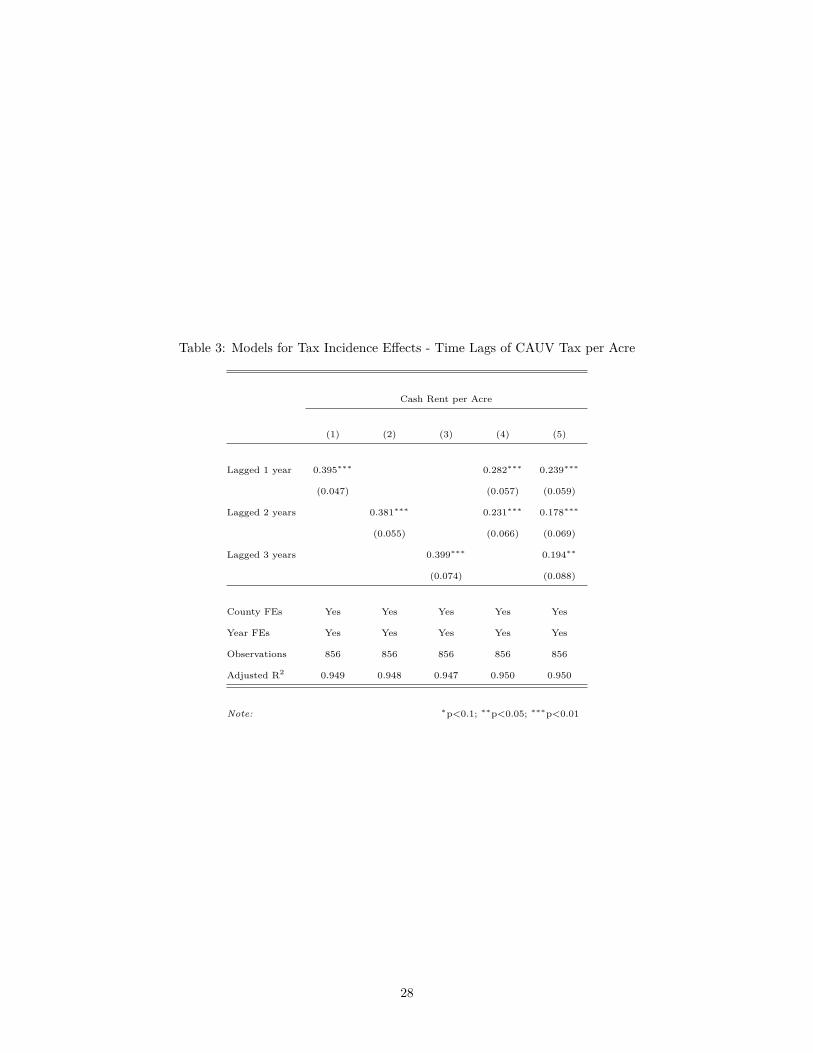
Table 3: Models for Tax Incidence Effects - Time Lags of CAUV Tax per Acre

Cash Rent per Acre

(1) (2) (3) (4) (5)

Lagged 1 year 0.395∗∗∗ 0.282∗∗∗ 0.239∗∗∗

(0.047) (0.057) (0.059)

Lagged 2 years 0.381∗∗∗ 0.231∗∗∗ 0.178∗∗∗

(0.055) (0.066) (0.069)

Lagged 3 years 0.399∗∗∗ 0.194∗∗

(0.074) (0.088)

County FEs Yes Yes Yes Yes Yes

Year FEs Yes Yes Yes Yes Yes

Observations 856 856 856 856 856

Adjusted R2 0.949 0.948 0.947 0.950 0.950

Note: ∗p<0.1; ∗∗p<0.05; ∗∗∗p<0.01

28

$0

$1,000

$2,000

$3,000

$4,000

$5,000

1991 2000 2010 2017

100

90 to 99

80 to 89

70 to 79

60 to 69

50 to 59

0 to 49

in 2016 dollars per acre, average value in black

CAUV for Cropland by Productivity Index

Source: Ohio Department of Taxation

Figure 1:

Figures

29

$0

$50

$100

$150

1994 2000 2010 2017

Cash Rental Rate

Property Tax

in 2016 dollars per acre

Cash Rent and CAUV Tax Trends in Ohio

Sources: USDA−NASS and Ohio Department of Taxation

Figure 2:

30

Demand

Tax paid by renters

Tax paid by owners

Supply w/o Tax

Supply w/Tax

Rented Land

Cash Rent

Market for Rented Farmland

Figure 3:

31

$0

$50

$100

$150

$200

per acre, in 2017

Cash Rent for Cropland

0%

40%

80%

120%

from 2009 to 2017

Change in Cash Rent for Cropland

$0

$25

$50

$75

$100

per acre, in 2016

CAUV Property Tax

0%

100%

200%

300%

400%

2008 to 2016

Change in CAUV Property Tax

Figure 4:

32

Appendix - CAUV Calculation

Regardless of the type of commodity a farmer produces (crops, livestock, aquaculture, etc.), the CAUV value

for the land is determined solely based on its soil type and a formula from ODT which attempts to represent

the expected use-value of agricultural land for an average farmer in Ohio. For each of the over 3,500 soil

types (s) in Ohio, a particular year’s (t) CAUV value is calculated as the net operating income for this type

of soil divided by the capitalization rate:

CAUVs,t = NOIs,t

CAPt(4)

where CAPt represents the capitalization rate and NOIs,t represents the net operating income. Prior to 2015,

the capitalization rate was based on a 60% loan and 40% equity appreciation with interest rates for each

value based on a 7-year Olympic average17 where the value for the loan interest rate came from a 15-year

mortgage from Farm Credit Services (FCS) and the equity interest rate was the Federal Funds rate plus two

percentage points. For the 2015 tax year, the capitalization rate changed to an 80% loan (based on 25-year

mortgage from FCS) and 20% equity appreciation. In 2017, ODT changed the interest rate used for equity

appreciation to the 25-year average total rate of return on farm equity from USDA-ERS. The capitalization

rates used by the ODT in CAUV calculations since 2006 exhibit a steady decline from 8.5% to 6% until the

change in 2015 as seen in table 5.

Net operating income, NOIs,t, captures the average returns to an acre of land under normal management

practices which is adjusted by the state-wide rotation pattern of crops. This is defined as:

NOIs,t =∑

c

wc,t × (GOIs,c,t − nonlands,c,t) (5)

where c denotes the crop type, which is either corn, soybeans, or wheat18 which represent the dominant crops17An Olympic average is a simple mean after removing the highest and lowest value.18Prior to 2010, hay was used in this calculation but never represented more than 5% of the rotation. Hay was dropped due to

33

in Ohio and wc,t is crop’s share of state production. Each crop’s share of state production is based on a

5-year average of total production among the three crops with the weights summing to 1.19 The non-land

costs are represented by nonlands,c,t, which are calculated as 7-year Olympic averages for typical costs of

producing each crop. The Ohio State University Extension conducts annual surveys for costs of production

which serve as the yearly estimates to calculate a 7-year Olympic average for non-land costs. Prior to 2015,

the values in nonlands,c,t were lagged one year – i.e. tax year 2014 used the values from 2007 to 2013. From

2015 onward, the current year values are included in the nonlands,c,t calculations.

Gross operating income, GOIs,c,t, is based on historical yields and prices for each crop. The gross operating

income across each soil and crop type is defined as:

GOIs,c,t = Y ieldc,Ohio,t

Y ieldc,Ohio,1984× Y ieldc,s,1984 × Pricec,Ohio,t (6)

where Y ieldc,Ohio,t is a 10-year average for state-wide yields and Pricec,Ohio,t is a 7-year Olympic average

for state-wide prices. Prices are based on USDA-NASS data and are weighted based on state production to

further attempt to proxy revenues. Prior to 2015, both yield and price were lagged two years in its calculation

but the changes in 2015 decreased their lag to one year.

Each soil type has a corresponding base yield of production for each crop from 1984 – which is the most recent

comprehensive soil survey for the state of Ohio (Zobeck, Gerken, and Powell 1983). Prior to 2006, the ODT

did not adjust for yield trends and calculated gross operating income for each soil type via their 1984 yields

thus suppressing estimated revenues. ODT began adjusting for yield trends through the current method of

taking the Olympic average of state-wide yields (irrespective of soil type), dividing by the state-wide yields

for each crop in 1984, then multiplying this value based on the 1984 crop yield for the particular soil type

evaluated. The scaling factor for all soils and crops is the same, thus the only difference in yields for a soil is

due to their 1984 base yield. The values used in CAUV calculation can be seen in table 5

unreliable estimates of prices and yields.19Prior to 2010, the Ohio Farm Bureau set rotation percentages based on the slope of soil in an ad hoc method.

34

Table 4: Years Used in CAUV Calculation

Tax Year Capitalization Rate Yields Prices Non-Land Costs Rotation

2005 1999-2005 1984 1997-2003 1998-2004 ad hoc

2006 2000-2006 1995-2004 1998-2004 1999-2005 ad hoc

2007 2001-2007 1996-2005 1999-2005 2000-2006 ad hoc

2008 2002-2008 1997-2006 2000-2006 2001-2007 ad hoc

2009 2003-2009 1998-2007 2001-2007 2002-2008 ad hoc

2010 2004-2010 1999-2008 2002-2008 2003-2009 2004-2008

2011 2005-2011 2000-2009 2003-2009 2004-2010 2005-2009

2012 2006-2012 2001-2010 2004-2010 2005-2011 2006-2010

2013 2007-2013 2002-2011 2005-2011 2006-2012 2007-2011

2014 2008-2014 2003-2012 2006-2012 2007-2013 2008-2012

2015 2009-2015 2005-2014 2008-2014 2009-2015 2010-2014

2016 2010-2016 2006-2015 2009-2015 2010-2016 2011-2015

2017 2011-2017 2007-2016 2010-2016 2011-2017 2012-2016

All categories are Olympic averages except for rotation and yields.

35

Table5:

Values

Usedin

CAUV

Calcu

latio

n

Year

Cap

.Rate

CornYield

CornPr

ice

CornCost

SoyYield

SoyPr

ice

SoyCost

Wheat

Yield

Whe

atPr

ice

Whe

atCost

2006

8.50%

132

$1.99

$232.83

40$4.84

$167.50

63$2.49

$151.98

2007

8.40%

134

$1.96

$235.70

40$4.89

$168.14

64$2.64

$153.67

2008

8.30%

139

$2.02

$242.39

42$5.19

$174.44

67$2.89

$156.68

2009

7.90%

140.7

$2.29

$264.12

42$5.60

$175.21

66.7

$3.05

$159.01

2010

7.80%

140.1

$2.66

$286.65

41.2

$6.41

$189.10

67.1

$3.41

$170.16

2011

7.60%

144.9

$2.89

$300.98

42.5

$7.22

$204.60

67.3

$3.64

$192.94

2012

7.50%

146.5

$3.19

$350.71

43.1

$7.74

$227.51

66.2

$3.98

$211.52

2013

6.70%

148.5

$3.91

$391.90

43.7

$8.98

$248.69

65.3

$4.54

$230.62

2014

6.20%

151.9

$4.48

$437.85

45$10.13

$275.21

66$5.16

$255.48

2015

6.60%

155.2

$4.55

$516.99

46.7

$11.09

$325.42

67.1

$5.67

$296.98

2016

6.30%

156.2

$4.49

$524.47

47.2

$10.91

$336.33

66.7

$5.53

$323.52

2017

8.00%

156.2

$4.51

$538.78

47.9

$10.83

$347.10

67.9

$5.53

$336.21

Values

areba

sedoff

oftheform

ulametho

dsin

useat

thetim

ean

dareno

toffi

cial

USD

Avalues

forthegiventaxyear

atthetim

e.

36

Appendix - Additional Robustness Checks

One particular concern for data on cash rental rates is that only counties with higher levels of agricultural

production were surveyed in 2008, which might arguably be comprised of a different type of renter in Ohio.

To assess whether or not the sample of counties from 2008 produce drastically different results, table 6 repeats

the models of table 2 but only for the subset of counties which were surveyed in 2008. The point estimates on

property tax per acre are across the board lower for the subset of counties surveyed in 2008, although each

point estimate is within one standard deviation of each table’s counterpart. Within this subset, the preferred

specification implies an incidence rate of $0.31 passed onto renters from an additional $1 of property tax –

which is within the range of estimates for the agricultural incidence rate literature.

Another concern in relation to the cash rental rate variable is that the 2015 values do not exist and are

interpolated in the previous models. The linear interpolation procedure may provide spurious correlation

and needs to be addressed by re-estimating models which omit the 2015 values, however this comes with the

caveat that a year of observation is dropped which reduces precision of estimates. Table 7 re-estimates model

5 from table 2 as well as model 5 from the 2008 county subset from the first two models of table 6. While the

point estimates in the models with 2015 omitted are consistently higher, they are still within a reasonable

range based upon the standard errors for each estimate. While the interpolated procedure does not perfectly

reflect what occurred in 2015, the fairly consistent point estimates for the tax incidence rate are reflective of

a robust result for the tax incidence rate ranging between 0.31 and 0.40.

In addition, there may be concerns about the time periods for the main results especially as it relates to

the period around 2013 where agricultural land prices began to stagnate. As a robustness check, we present

models 3 and 4 in table 7 which use pre-2013 data and post-2012 data respectively. We caution against too

much interpretation here because of the nature of property tax changes in Ohio. Subsetting data by time

periods reduces the number of potential changes in property tax for counties. In a sample from 2008 through

2017, each county will cycle through 4 different CAUV values throughout this time period. Reducing the

time frame to 2008 to 2012 (or 2013 to 2017) results in about half the counties with 2 different CAUV values

37

and the other half with 3 different values. That stated, the period prior to 2013 has a higher incidence rate

than the full sample while the post-2012 sample results in an insignificant effect of property taxes on the cash

rental rate.

And finally, table 8 addresses concerns over potential trends in cash rents over time although similar to the

concerns of differing time periods we caution for interpreting this results due to the limited amount of changes

in CAUV values over this time. Model 1 is the same result at table 2 model 4 with our preferred specification

of county and year fixed effects with the full sample from 2008 to 2017. In model 2, year fixed effects are

replaced with a state-wide time trend and county fixed effects which results in a lessened incidence rate.

Model 3 replaces year fixed effects with individual county time trends – which largely mimics the property

tax variable of interest – and the resulting coefficient measuring tax incidence is an insignificant predictor

under this model. Model 4 includes both county and year fixed effects but further includes a time trend

at the agricultural reporting district, which lessens the estimated coefficient for tax incidence. And finally

model 5 removes county fixed effects but includes agricultural reporting district time trends which produces a

similar estimate for tax incidence as our preferred specification.

38

Table 6: Models for Tax Incidence Effects - Subset Of Counties with Cash Rent in 2008

Cash Rent per Acre

(1) (2) (3) (4) (5)

CAUV Tax per Acre 1.205∗∗∗ 1.345∗∗∗ 0.960∗∗∗ 0.314∗∗∗ 0.322∗∗∗

(0.084) (0.153) (0.042) (0.051) (0.051)

Effective Productivity Index 0.275

(0.363)

Government Payments 0.011

(0.094)

Mineral’s Share 0.115

(0.156)

Share Enrolled in CRP −2.605∗∗

(1.266)

State Share of Planted Corn 11.248∗∗∗

(4.319)

Nonland Costs 0.027

(0.033)

Population Density −0.004

(0.090)

Unemployment Rate −0.563

(0.539)

County FEs No No Yes Yes Yes

Year FEs No Yes No Yes Yes

Observations 640 640 640 640 640

Adjusted R2 0.291 0.333 0.872 0.943 0.945

Note: ∗p<0.1; ∗∗p<0.05; ∗∗∗p<0.01

39

Table 7: Models for Tax Incidence Effects - Time Period Subsets

Cash Rent per Acre

All, excl. 2015 Subset, excl. 2015 All, pre 2013 All, post 2012

(1) (2) (3) (4)

CAUV Tax per Acre 0.432∗∗∗ 0.356∗∗∗ 0.464∗∗∗ 0.036

(0.067) (0.071) (0.149) (0.042)

Effective Productivity Index 0.220 0.428 −0.273 0.250

(0.308) (0.403) (0.271) (0.250)

Government Payments 0.061 0.071 0.175∗ 0.015

(0.110) (0.117) (0.099) (0.066)

Mineral’s Share −0.265 0.158 −1.835 0.139

(0.182) (0.160) (11.748) (0.120)

Share Enrolled in CRP −2.603∗ −2.199 1.081 −1.081

(1.574) (1.504) (2.956) (1.603)

State Share of Planted Corn 8.615∗∗ 11.625∗∗ 1.743 −2.675

(3.604) (4.597) (3.598) (4.036)

Nonland Costs 0.037∗ 0.037 0.001 −0.027

(0.020) (0.037) (0.016) (0.021)

Population Density 0.004 0.010 −0.044 0.113

(0.039) (0.093) (0.043) (0.094)

Unemployment Rate −1.170∗∗ −0.603 −1.167∗∗∗ 1.097

(0.483) (0.531) (0.416) (1.011)

County FEs Yes Yes Yes Yes

Year FEs Yes Yes Yes Yes

Observations 768 576 416 440

Adjusted R2 0.948 0.942 0.965 0.983

Note: ∗p<0.1; ∗∗p<0.05; ∗∗∗p<0.01

40

Table 8: Models for Tax Incidence Effects - Trends

Cash Rent per Acre

(1) (2) (3) (4) (5)

CAUV Tax per Acre 0.395∗∗∗ 0.261∗∗∗ −0.088 0.175∗∗∗ 0.438∗∗∗

(0.047) (0.057) (0.078) (0.050) (0.086)

County FEs Yes Yes Yes Yes No

Year FEs Yes No No Yes Yes

Trends No Statewide County Reporting District Reporting District

Observations 856 856 856 856 856

Adjusted R2 0.949 0.922 0.948 0.961 0.772

Note: ∗p<0.1; ∗∗p<0.05; ∗∗∗p<0.01

41