Properties of Small Metallic Particles

Helen Chappell, Aikaterina Plati, Yi Shen 18th December 2002

Supervisors: Professor Harry Bhadeshia, Dr Thomas Sourmail

Phase Transformations and Complex Properties Research Group, Department

of Materials Science and Metallurgy, University of Cambridge.

1.Introduction

Small particles have long been studied in metallurgy because many properties, such as

melting temperature, depend on particle size. With the advent of new

nanotechnologies, the study of such particles has become even more relevant.

This project has involved modelling the effects on melting temperature with respect to

changes in particle size, shape, crystal structure and chemical composition.

Using a sketch of temperature against Gibbs free energy, the melting temperature of a

solid, Tm, can be found from plotting a line for GS, the Gibbs free energy of the solid,

and a line for GL, the Gibbs free energy of the liquid; their intersection giving the

melting temperature of the solid. That is, for a flat interface at Tm,

GL= GS (1)

However, for the curved interface of a small particle, the melting temperature is

reduced. For this case, at Tmr,

GL = GS + σ ds/dn (2)

where ds/dn is the increase in surface are per atom added and σ the interfacial energy.

This surface area depends on the shape of the particle. This is illustrated in Figure 1.

In order to investigate these variations in melting temperature, the project was

organised into three parts.

1. The first part of the project involved the modelling of pure iron particles.

Calculations of melting temperatures were carried out for both spherical and

cylindrical particles and this was done for both a face-centred cubic structure

(austenite) and a body-centred cubic structure (ferrite). For these four different

sets of conditions, particle radius was varied from 1×10-9 m to 1×10-7 m and

the new melting temperatures recorded.

2. The second part of the project involved modelling these same variations in

melting temperature, but this time for the ferritic and austenitic phases of iron

in a nickel-iron alloy of 10-wt% nickel, for the case where both liquid and

solid have identical composition.

3. The third part of the project involved a statistical analysis of the composition

of a sample of atoms taken from a fixed volume of the 10-wt% nickel- iron

alloy. This analysis allowed a distribution of melting temperatures as a

function of particle radius to be created. That is, for any random sample of

atoms chosen from a fixed volume of known composition, a distribution of

melting temperatures was created based on the statistical probability of the

composition of that chosen sample.

2.Nomenclature

GL - Gibbs free energy of liquid phase

GS - Gibbs free energy of solid phase

GSR – Gibbs free energy of small particle phase

Tm – melting temperature

Tmr – revised melting temperature with small particles

r – radius of particle

Vm – molar volume of solid

σ − interfacial energy per unit area

N – Avogadro’s number (6.022 ×10 23 mol –1)

a – lattice parameter

α − thermal expansion coefficient

l0 – length of cell parameter at 273K

lt - transformed length of cell parameter at given temperature

Na – number of atoms in a particle

Np - number of particles

f – probability of finding a nickel atom in a given sample of a nickel-iron alloy

3.Materials and Methods

3.1 MTDATA

The thermodynamic calculations were all carried out using a commercially available

software package and database. MTDATA is a software package, first created in 1970

at the National Physical Laboratory. It contains a vast amount of critically assessed

thermodynamic data that can be used in the calculation of phase equilibria in

multiphase and multicomponent systems [1,2]. The program minimises the Gibbs free

energy of a system, thereby calculating the equilibrium composition and volume

fractions of the phases present. Any phase may be suppressed in these calculations

and the calculations re-run.

The thermodynamic data needed to do this are found in the SGTE database. For

larger systems where data are not available thermodynamic theory is used to make

predictions. Although this program can give extremely useful data it says nothing of

the kinetics of phase formation [3]. This package was used in all three parts of the

project to find Gibbs free energy values at varying temperatures. Table 1 shows the

phases for which these data were collected.

Phase Iron Nickel-Iron AlloyBCC_A1 ferrite GS GSFCC_A2 austenite GS GSLiquid GL GL

Table 1. Data retrieved from MTDATA

These calculations were run for one mole of the given substance, with temperature

ranging from 573–1973 K, stepped by two-Kelvin intervals.

3.2 Excel

The Excel statistical package was used to create graphs of the figures obtained from

MTDATA, and to fit polynomial equations to these data. These equations were then

used for the calculation of melting temperature as a function of particle radius, as

described in Section 1, using the Curvefit3 program developed in this project.

3.3 Curvefit3

Curvefit3 is a program written in FORTRAN 77 to find the melting temperature of

particles of different radii, which have a fixed composition. These data were again

transferred to Excel files so plots of particle radii against melting temperature for a

given interfacial energy value, could be generated. Figure 2 shows a flow diagram

explaining the function of this program. The program transcript is given in Appendix

1.

Figure

Decide the radius

Try BD

A = (min T )

C = (max T )

Y

DGB < 1.0 N DGA × DGB<0 N

Y

= (min T + max T)/2GB= GLB - GSRB

(min T)=A(max T)=B

(min T)=B(max T)=A

Write

Calculate from polynomial equationsGLA, GSRB, GLC, GSRC, DGA = GLA– GSRA,DGC = GLC– GSRC

2. Flowchart for Curvefit3

3.4 Try

Try is a program written for this project in FORTRAN 77 [4]. This program was used

for the third part of the project. It finds the range of possible compositions for a

specific number of atoms taken from a sample of fixed composition and fixed volume.

It then tabulates these compositions with melting temperature. The results are

produced in the form of sample radius against melting temperature. This program

allowed for different values of σ and different compositions to be specified. For our

specific calculations, using the nickel-iron alloy, a fixed composition of 10-wt%

nickel was used and the value of σ was varied from 0.1 to 0.5 Jm-2. Figure 3 shows a

flow diagram explaining the function of this program. The program transcript is given

in Appendix 1.

Chart A

Chart A

Chart A

DG

Y

Decide σ

Define radius ( r )

Convert it toNumber of atoms (NA)Find σx

Find lowercomposition

Find highercomposition

A =

Try B = (min Get from dataFind GSRBDGB= GLB - G

Set (min T )

C = (max T )

Y

B < 1.0 N DGA × DGB<0 N

Figure 3.Flowchart for TRY

T + max T)/2base: GLB ,GSB

SRB

(min T)=A(max T)=B

(min T)=B(max T)=A

Write: σ, radius, melting temperature

Get from data base : GLA, GSB, GLC, GSC,Find:GSRB, , GSRC, DGA = GLA– GSRA,DGC = GLC– GSRC

Write: σ, Radius,Higher melting temperature

Write: σ, Radius,Lower melting temperature

4.Results and Discussion

4.1 Iron Particles

For the data collected from MTDATA for this system, it was found that second order

polynomial equations made the best fit with correlation coefficients of R =1. These

equations are given in Table 2.

GS (kJ/mol)– ferrite GS (kJ/mol) – austenite GL(kJ/mol)y = -0.0176T2 – 31.274T +6207.5

y = -0.014T2 – 41.2827T +13818

y = -0.0146T2 – 47.827T +26339

Table 2. Polynomial equations for iron data, where T is temperature

As is discussed in Section 1,

GSR = GS + σ ds/dn (3)

For a spherical particle, ds/dn is given by 2Vm/r, where Vm is the molar volume and r

the radius of the particle. Thus, GSR, the Gibbs free energy of the particle phase, is

given by,

GSR = GS + σ 2Vm/r (4)

2Vm/r is derived as follows:

dV = dnVm,

where V is particle volume.

Therefore, dn = dV/Vm

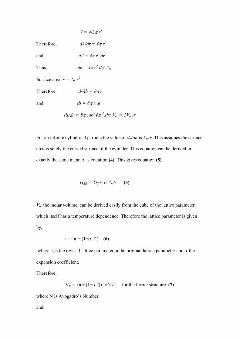
V = 4/3π r3

Therefore, dV/dr = 4π r2

and, dV = 4π r2.dr

Thus, dn = 4π r2.dr/ Vm

Surface area, s = 4π r2

Therefore, ds/dr = 8π r

and ds = 8π r.dr

ds/dn = 8πr.dr/ 4πr2.dr/ Vm = 2Vm /r

For an infinite cylindrical particle the value of ds/dn is Vm/r. This assumes the surface

area is solely the curved surface of the cylinder. This equation can be derived in

exactly the same manner as equation (4). This gives equation (5).

GSR = GS + σ Vm/r (5)

Vm, the molar volume, can be derived easily from the cube of the lattice parameter

which itself has a temperature dependence. Therefore the lattice parameter is given

by,

at = a + (1+α T ) (6)

where at is the revised lattice parameter, a the original lattice parameter and α the

expansion coefficient.

Therefore,

Vm = (a + (1+αT))3 ×N /2 for the ferrite structure (7)

where N is Avogadro’s Number.

and,

Vm = (a + (1+αT))3 ×N /4 for the austenite structure (8)

Values for a were taken from [4]. Table 3 gives the equations for GSR for both

spherical and cylindrical particles of the austenite structure and the ferrite structure.

Ferrite AusteniteSpherical particles GSR (kJ/mol) = Gs + σ(2×

(a + (1+1.18e−6T))3 ×N/2)/r

GSR (kJ/mol) = Gs + σ(2×(a + (1+1.8e-6T))3 ×N/4)/r

Cylindrical particles GSR (kJ/mol) = Gs + σ× (a+ (1+1.18e−6T))3 × N/2)/r

GSR (kJ/mol) = Gs + σ × (a+ (1+1.8e−6T))3 × N/4)/r

Table 3. GSR equations for iron particles

Using these equations in Curvefit3, the following results were generated. Figure 4

shows the results for ferritic spherical particles, Figure 5 the results for austenitic

spherical particles, Figure 6 the results for ferritic cylindrical particles and Figure 7

the results for austenitic cylindrical particles. All these plots have been constructed

with 1/r on the x-axis for clarity.

The first thing to note in these results is the maximum melting temperatures for the

two different compositions. Looking at Figures 4 and 5 it can be seen that the

maximum melting temperature for the ferrite structure is 1811.45 K but this

temperature is reduced by approximately 150 K to 1661.41 K in the austenite

structure. This observation can be explained be reference to the density of the two

crystal structures. The ferrite structure, unlike that of the austenite, is not close

packed. This structure is thus less dense. The effect of this reduced density is an

increased entropy term at higher temperature, which reduces the Gibbs free energy.

Therefore, the ferrite structure is stable to higher temperatures than the austenite [6].

It is also true that the austenite structure has a broader range of melting temperatures,

1548.63 K separating the highest and lowest temperatures, compared to a difference

of just 1419.57 K for the ferrite structure.

The charts are plotted such that each line represents the use of a different interfacial

energy value. In all cases, the larger this value the lower the melting temperature. This

observation is true for both spherical and cylindrical particles.

The reason for this is that the value of GSR would be made less negative as the

additional Gibbs energy given by ds/dn is a positive quantity. Because the Gibbs

energy of the system is increased for a given temperature, the melting temperature

will decrease in order to minimise the energy of the system. That is, the liquid phase

has a lower Gibbs energy than the particle phase at higher temperatures.

Additionally, ds/dn is increased by decreasing the radius of the particle, as is evident

from equation (4). Thus, once again, the Gibbs free energy is increased and the

melting temperature is reduced. This is true for both spherical and cylindrical

particles.

Turning to Figures 6 and 7, the most obvious observation is the decreased range of

melting temperatures. For example, the difference in Tmr at its greatest (i.e. the

smallest radius) is just 817.01 K for the austenitic cylindrical particles. This compares

to a range of 1548.63 K for the spherical particles. Naturally, this is a consequence of

the factor of 2, which is missing from equation (5), as compared to equation (4). This

shows that the spherical particle maximises the curved interface for a particle of a

given radius.

4.2 Nickel-Iron Alloy Particles

The same analysis was carried out with a 10-wt% nickel-iron alloy. For the data

collected from MTDATA , it was again found that second order polynomial equations

made the best fit, with the R value equal to 1. These equations are given in Table 4.

GS (kJ/mol) – ferrite GS (kJ/mol) – austenite GL (kJ/mol)y = -0.0172T2 – 35.564T +7602.5

y = -0.0141T2 – 44.14T +12886

y = -0.0146T2 – 50.209T +25307

Table 4. Polynomial equations for alloy data, where T is temperature

The GSR equations are the same as those for the iron particles, as given in Table 3.

Curvefit3 produced the following results. Figure 8 shows the results for ferritic

spherical particles, Figure 9 the results for austenitic spherical particles, Figure 10 the

results for ferritic cylindrical particles and Figure 11 the results for austenitic

cylindrical particles.

The first thing to note here is that the melting temperature for σ = 0.0 Jm-2 in the

alloy, is higher for the austenite crystal structure than for the ferrite crystal structure

as can be seen on Figures 8 and 9. The difference is small with an austenite Tm of

1784.3 K and a ferrite Tm of 1756.84 K. This is in contrast to a pure iron sample where

the austenite structure has a much lower Tm value. This occurs because the nickel

atoms in the structure stabilize the austenitic form relative to the ferritic form.

However, despite this difference, the austenite structure, as with pure iron, has a

broader range of melting temperatures than the ferrite structure. Comparing the range

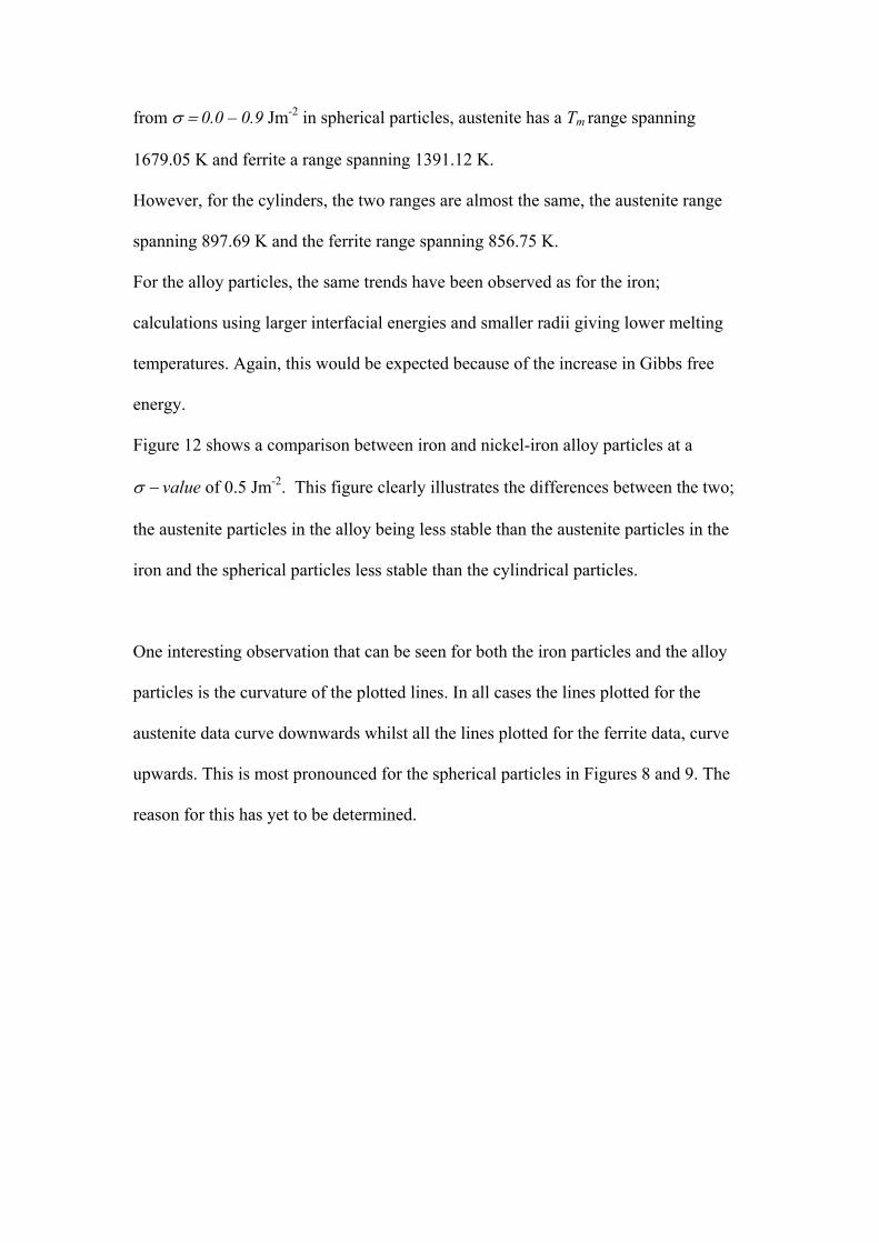
from σ = 0.0 – 0.9 Jm-2 in spherical particles, austenite has a Tm range spanning

1679.05 K and ferrite a range spanning 1391.12 K.

However, for the cylinders, the two ranges are almost the same, the austenite range

spanning 897.69 K and the ferrite range spanning 856.75 K.

For the alloy particles, the same trends have been observed as for the iron;

calculations using larger interfacial energies and smaller radii giving lower melting

temperatures. Again, this would be expected because of the increase in Gibbs free

energy.

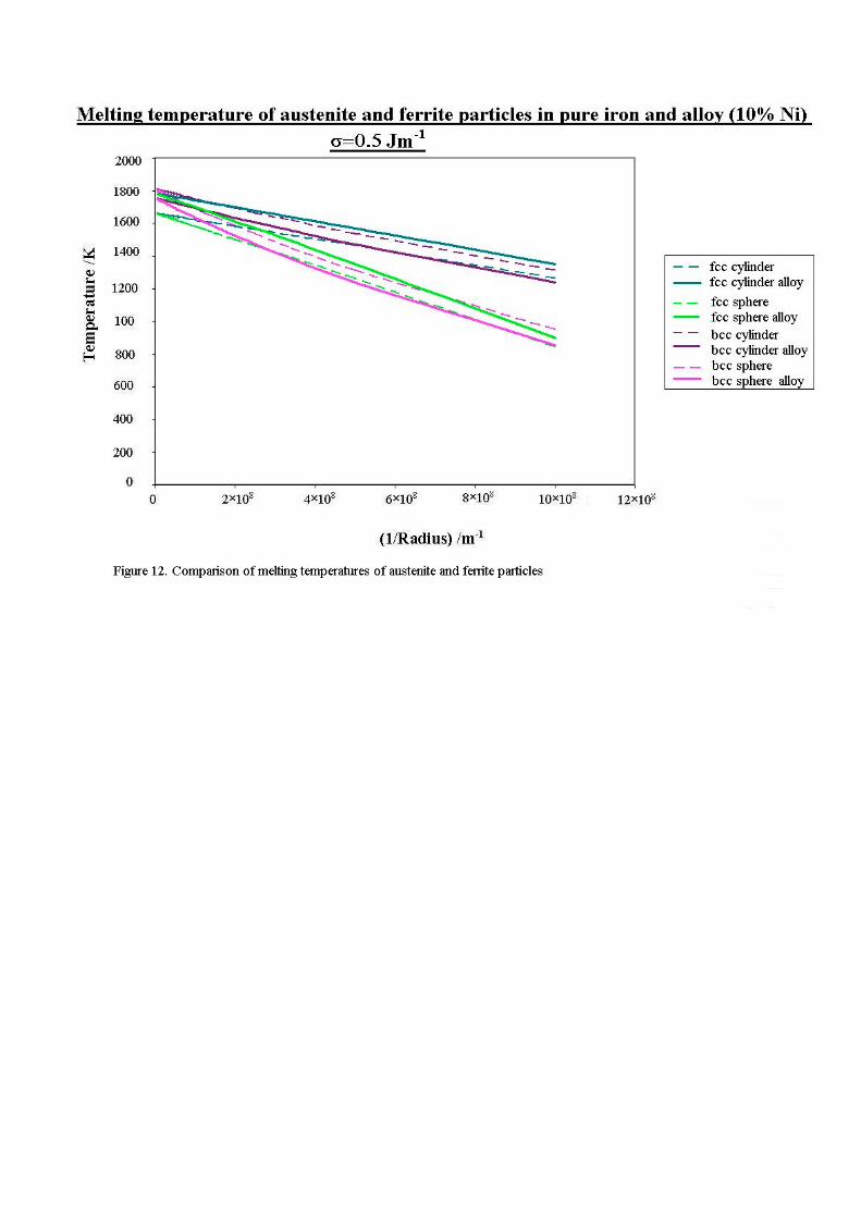
Figure 12 shows a comparison between iron and nickel-iron alloy particles at a

σ − value of 0.5 Jm-2. This figure clearly illustrates the differences between the two;

the austenite particles in the alloy being less stable than the austenite particles in the

iron and the spherical particles less stable than the cylindrical particles.

One interesting observation that can be seen for both the iron particles and the alloy

particles is the curvature of the plotted lines. In all cases the lines plotted for the

austenite data curve downwards whilst all the lines plotted for the ferrite data, curve

upwards. This is most pronounced for the spherical particles in Figures 8 and 9. The

reason for this has yet to be determined.

4.3 Statistical Analysis of Composition and Melting Temperature

For this part of the project a 10-wt% nickel-iron alloy was used in the calculations. It

was assumed that the volume of our sample from which a particle of a given radius

would be picked, would remain constant. That is,

Np× Na = constant

where Np is the number of particles and Na is the number of atoms.

For this fixed composition, the distribution, showing the fractional composition of

nickel within a chosen sample will be binomial and the standard deviation will

therefore be,

σx = √Na ×f(1-f) (9)

where σx is the standard deviation and f the probability of finding a nickel atom in a

given sample of nickel-iron alloy.

Thus the fractional composition of nickel in a particle will be between 0.1 + σx and

0.1 - σx. Na in equation (9) is given by equation (10).

Na = (4/3π r3)/ Vm × N (10)

Equation (10) allows the composition of a particle to be found simply from the radius

of that particle. Therefore, the TRY program was used to find these distributions of

composition, as given by the radius of the sample particle and this was correlated with

the corresponding melting temperatures. It was then possible to plot radius against

melting temperature. This gave two lines, one corresponding to the maximum nickel

composition and one corresponding to the minimum nickel composition for a given

radius. The true melting temperature would probably lie somewhere in between these

two. Figure 13 shows these results for a fixed composition of 10-wt% nickel, varying

the interfacial energy, σ, from 0.1 to 0.5 Jm-2.

These results show that there is only a significant difference in melting temperatures

between the maximum and minimum nickel composition when the radius of the

particle is extremely small. Any particle with a radius greater than approximately

2×10-8 m will essentially have a constant melting temperature. Only for very small

sample sizes is the compositional uncertainty of consequence.

5. Conclusion

During the course of this project a number of interesting observations were recorded.

Firstly, it is evident that spherical particles have the greatest effect on melting

temperature of a sample. This indicates that the sphere maximises the curved surface

interface. Cylindrical particles also reduce the melting temperature but to a lesser

extent.

Secondly, the factors that decrease the melting temperature are 1) an increase in

interfacial energy and 2) a decrease in particle radius. Thus, the lowest melting

temperatures are found with extremely small particles and a large interfacial energy.

For the 10-wt% nickel-iron alloy, the same effects are observed but the reduction in

melting temperature spans a narrower range than for the pure iron particles.

The third part of the project revealed that the melting temperature of a sample particle

would be practically constant except for extremely small particles of less than 2×10-8

m.

Hopefully, these results will be used in future research.

6.Acknowledgments

With thanks to Harry. Aussi, un grand merci à Thomas pour son aide, sa patience et

surtout, pour ses chocolats!

7. References

1. http://www.npl.co.uk/npl/cmmt/mtdata/mtdata.html

2. Davies R H, Dinsdale A T, Hodson S M, Gisby J A, Pugh N J, Barry T I,

Chart T G, Proc. Conf. "User Aspects of Phase Diagrams", 25-27 June 1990,

Petten, Institute of Metals. "MTDATA - The NPL databank for

metallurgical thermochemistry".

3. Yescas Gonzalez, M.A. (2001). Modelling the Properties of Austempered

Ductile Cast Iron. Pages 109-110. University of Cambridge.

4. Thomas Sourmail. (2002). Try.

5. www.liv.ac.uk/~goodhew/CubicStructures_Hout.doc

6. Cottrell, A. (1988). Introduction To The Modern Theory of Metals. Institute of

Metals.

8. Appendix 1

8.1 Curvefit3

PROGRAM CURVEFIT implicit none INTEGER I,J DOUBLE PRECISION VCELL,AVOGA DOUBLE PRECISION RADIUS,TEMPA,GS,GL,GSR,TEMPB,TEMPC DOUBLE PRECISION GSA,GSB,GSC,GLA,GLB,GLC,GSRA,GSRB,GSRC DOUBLE PRECISION DGA,DGB,DGC,VCELLA,VCELLB,VCELLC DOUBLE PRECISION SIGMA,DEPS

WRITE(*,*) WRITE(*,*) "Enter sigma:" READ(*,*) SIGMA AVOGA=6.0221E23 DEPS=1.0 DO 10 I=1,200 TEMPA=0.0 TEMPB=1973.0 3 TEMPC=(TEMPA+TEMPB)/2c WRITE(*,*) TEMPC RADIUS=DBLE(I)*1e-09 GSA=-0.0172*(TEMPA**2)-35.564*TEMPA+7602.5 GSB=-0.0172*(TEMPB**2)-35.564*TEMPB+7602.5 GSC=-0.0172*(TEMPC**2)-35.564*TEMPC+7602.5 GLA=-0.0146*(TEMPA**2)-50.209*TEMPA+25307 GLB=-0.0146*(TEMPB**2)-50.209*TEMPB+25307 GLC=-0.0146*(TEMPC**2)-50.209*TEMPC+25307 VCELLA=(2.86E-10*(1+(1.18E-6)*TEMPA))**3 VCELLB=(2.86E-10*(1+(1.18E-6)*TEMPB))**3 VCELLC=(2.86E-10*(1+(1.18E-6)*TEMPC))**3 GSRA=GSA+(SIGMA*(VCELLA*AVOGA/2.)/RADIUS) GSRB=GSB+(SIGMA*(VCELLB*AVOGA/2.)/RADIUS) GSRC=GSC+(SIGMA*(VCELLC*AVOGA/2.)/RADIUS) DGA=GLA-GSRA DGB=GLB-GSRB

DGC=GLC-GSRCc WRITE(*,*) DGA,DGC,DGB IF ((DGA*DGC).lt.0) then TEMPA=TEMPA TEMPB=TEMPC ELSE TEMPA=TEMPC TEMPB=TEMPB ENDIF IF (DABS(DGB).GT.DEPS) GOTO 3 5 write(*,100) RADIUS,TEMPC,GSC,GSRC,GLC 10 continue

100 FORMAT(E12.6,4(1x,E12.6))

end

8.2 TRY

PROGRAM TRY

INCLUDE 'DIRUSRAP.FOR'

INTEGER IMODE,IERR,N,J,K,L CHARACTER*20 FILNAM,FIL2 CHARACTER*20 PI,PII,FAKE INTEGER CHOICE,I,II,ITER DOUBLE PRECISION AVOGA DOUBLE PRECISION NA,STDEV,COMPO(2) DOUBLE PRECISION TEMP,PRESS DOUBLE PRECISION RADIUS,SIGMA,MOLV,CAVER DOUBLE PRECISION TSOL(2) DOUBLE PRECISION HTEMP(4),GS(4),GL(4),DG(4),DEPS

CHOICE=2 I=1 II=2 AVOGA=6.02E23 IMODE=0 IERR=0 FAKE='' FIL2='def' PI='BCC_A2' PII='LIQUID' TEMP=1273.0

CALL MTDATA_RESERVE_UNIT(12)

OPEN(UNIT=1,FILE='input') READ(1,*) FILNAM READ(1,*) RADIUS READ(1,*) SIGMA READ(1,*) MOLV READ(1,*) CAVER READ(1,*) DEPS CLOSE(1)

OPEN(UNIT=12,FILE='results') WRITE(12,*) "Using mpi file: ",FILNAM WRITE(12,*) "Melting temperature between ",PI," and ",PII WRITE(12,*) "For an interfacial energy of ",SIGMA," J/mol" WRITE(12,*) "Average composition: ",CAVER WRITE(12,*) "With molar volume ",MOLV," m3/mol" WRITE(12,*) "Gibbs energies equal within +- ",DEPS

CALL INITIALISE_MTDATA(IMODE) CALL SGUMEN(1) CALL SGUMEN(2) CALL MTOPTN(IMODE,'STAGE_1=NEW') CALL OPEN_MPI_FILE(FILNAM,FIL2,IERR) CALL DISP_PHASES() CALL SET_PRINT_LEVEL(-2)

DO 100 K1=0,2 DO 110 K2=1,20

RADIUS=5.0e-10*(10.**DBLE(K1))*DBLE(K2)

NA=(4.*3.14159/3.)*(RADIUS**3) NA=NA*AVOGA/MOLV STDEV=DSQRT(NA*CAVER*(1.-CAVER))

COMPO(1)=((NA*CAVER)-STDEV)/NA COMPO(2)=((NA*CAVER)+STDEV)/NA WRITE(*,*) "COMPO LOWER: ",COMPO(1) WRITE(*,*) "COMPO UPPER: ",COMPO(2) PRESS=2.0*SIGMA*MOLV/RADIUS

PAUSE

DO 120 L=1,2 ITER=0 HTEMP(1)=273.0 HTEMP(3)=1973.0 CALL SET_INIT_COMPONENT_AMOUNT(I,COMPO(L)) CALL SET_INIT_COMPONENT_AMOUNT(II,(1.-COMPO(L)))C------------- start loop 5 HTEMP(2)=0.5*(HTEMP(1)+HTEMP(3)) ITER=ITER+1 DO 10 J=1,3 CALL SET_TEMPERATURE(HTEMP(J)) CALL ONLYNORM(PI,FAKE) CALL COMPUTE_EQUILIBRIUM() CALL DISP_RESULT(CHOICE) GS(J)=GIBBS_ENERGY_OF_PHASE(I)+PRESS WRITE(*,*) "GS: ",GS(J) CALL ONLYNORM(PII,FAKE) CALL COMPUTE_EQUILIBRIUM() CALL DISP_RESULT(CHOICE) GL(J)=GIBBS_ENERGY_OF_PHASE(I) WRITE(*,*) "GL: ",GL(J) DG(J)=GL(J)-GS(J) 10 CONTINUEC------------- if sign change between first two,C------------- select upper limit as middle IF (DG(2)*DG(1).LE.0.0) THEN HTEMP(3)=HTEMP(2) ELSE HTEMP(1)=HTEMP(2) ENDIF

IF(DABS(DG(2)).GT.DEPS.AND.ITER.LT.5000) GOTO 5 TSOL(L)=HTEMP(2) 120 CONTINUE WRITE(12,*) RADIUS,TSOL(1),TSOL(2) 110 CONTINUE 100 CONTINUE

CLOSE(12) END

C**********************************************************************C Subroutine ONLYNORMC This subroutine classifies normal the phase whose names areC passed as arguments and absent all the others.

SUBROUTINE ONLYNORM(PI,PII)

CHARACTER*20 PI,PII CHARACTER*20 PVAR CHARACTER*20 INIT_PHASE_NAME INTEGER INIT_NO_OF_PHASES

DO 10 I=1,INIT_NO_OF_PHASES() PVAR=INIT_PHASE_NAME(I)

IF (PVAR.EQ.PI .OR. PVAR.EQ.PII) THEN CALL SET_INIT_PHASE_CLASS(I,1) ELSE CALL SET_INIT_PHASE_CLASS(I,0) ENDIF 10 CONTINUE END

C********************************************************************C Subroutine DISP_RESULT(K)C displays the result of the last equilibrium calculationC argument K: 1/ mass of phases and compositions in wt%C 2/ moles of phases and compositions in mole fraction

SUBROUTINE DISP_RESULT(K)

INCLUDE 'DIRUSRAP.FOR'

INTEGER K,I,J,L,M,N

L=ACT_NO_OF_COMPONENTS() WRITE(*,*) EQUIL_NO_OF_PHASES() WRITE(*,*)

IF (K.EQ.1) THEN WRITE(*,*)'Weight and components weight fractions' WRITE(*,300) DO 10 I=1,EQUIL_NO_OF_PHASES() N=PHASE_PRESENT_AT_EQUILIBRIUM(I)

IF (L.GT.5) THEN WRITE(*,100) ACT_PHASE_NAME(N), & (ACT_COMPONENT_NAME(J), J=1,5) WRITE(*,200) MASS_IN_PHASE(N,2), & (COMPONENT_W_OF_PHASE(J,N,2), J=1,5) WRITE(*,*) ELSE WRITE(*,100) ACT_PHASE_NAME(N), & (ACT_COMPONENT_NAME(J), J=1,ACT_NO_OF_COMPONENTS()) WRITE(*,200) MASS_IN_PHASE(N,2), & (COMPONENT_W_OF_PHASE(J,N,2), J=1,ACT_NO_OF_COMPONENTS())

GOTO 21 ENDIF

IF (L.GT.10) THEN WRITE(*,400) (ACT_COMPONENT_NAME(J),J=6,10) WRITE(*,500) (COMPONENT_W_OF_PHASE(J,N,2), J=6,10) WRITE(*,*) ELSE M=6 GOTO 20 ENDIF

IF (L.GT.15) THEN WRITE(*,400) (ACT_COMPONENT_NAME(J),J=11,15) WRITE(*,500) (COMPONENT_W_OF_PHASE(J,N,2), J=11,15) WRITE(*,*) ELSE M=11 GOTO 20 ENDIF

20 WRITE(*,400) & (ACT_COMPONENT_NAME(J), J=M,ACT_NO_OF_COMPONENTS()) WRITE(*,500) & (COMPONENT_W_OF_PHASE(J,N,2), J=M,ACT_NO_OF_COMPONENTS())

21 WRITE(*,300) WRITE(*,*) 10 CONTINUE ENDIF

IF (K.EQ.2) THEN WRITE(*,*)'Moles and components mole fractions' WRITE(*,300) DO 30 I=1,EQUIL_NO_OF_PHASES() N=PHASE_PRESENT_AT_EQUILIBRIUM(I)

IF (L.GT.5) THEN WRITE(*,100) ACT_PHASE_NAME(N), & (ACT_COMPONENT_NAME(J), J=1,5) WRITE(*,200) MOLES_OF_COMPONENTS_IN_PHASE(N,2), & (COMPONENT_X_OF_PHASE(J,N,2), J=1,5) WRITE(*,*) ELSE WRITE(*,100) ACT_PHASE_NAME(N), & (ACT_COMPONENT_NAME(J), J=1,ACT_NO_OF_COMPONENTS()) WRITE(*,200) MOLES_OF_COMPONENTS_IN_PHASE(N,2), & (COMPONENT_X_OF_PHASE(J,N,2), J=1,ACT_NO_OF_COMPONENTS()) GOTO 41 ENDIF

IF (L.GT.10) THEN WRITE(*,400) (ACT_COMPONENT_NAME(J),J=6,10) WRITE(*,500) (COMPONENT_X_OF_PHASE(J,N,2), J=6,10) WRITE(*,*) ELSE M=6 GOTO 40 ENDIF

IF (L.GT.15) THEN

WRITE(*,400) (ACT_COMPONENT_NAME(J),J=11,15) WRITE(*,500) (COMPONENT_X_OF_PHASE(J,N,2), J=11,15) WRITE(*,*) ELSE M=11 GOTO 40 ENDIF

40 WRITE(*,400) & (ACT_COMPONENT_NAME(J), J=M,ACT_NO_OF_COMPONENTS()) WRITE(*,500) & (COMPONENT_X_OF_PHASE(J,N,2), J=M,ACT_NO_OF_COMPONENTS())

41 WRITE(*,300) WRITE(*,*)

30 CONTINUE ENDIF

100 FORMAT (1X,A,1X,5(5X,A,4X)) 200 FORMAT (E11.6,1X,5(1X,F9.7,1X)) 300 FORMAT (66('-')) 400 FORMAT (12X,5(5X,A,4X)) 500 FORMAT (12X,5(1X,F9.7,1X))

END

C *******************************************************************C Subroutine DISP_COMPONENTSC argument CHOICE: 1 / name of initial componentsC 2 / mass of initial componentsC 3 / moles of initial componentsC 4 / name of active components (after eq calc only)

SUBROUTINE DISP_COMPONENTS(CHOICE)

INTEGER CHOICE

DOUBLE PRECISION INIT_COMPONENT_MASS DOUBLE PRECISION INIT_COMPONENT_MOLES INTEGER ACT_NO_OF_COMPONENTS CHARACTER*20 INIT_COMPONENT_NAME,ACT_COMPONENT_NAME

WRITE(*,*)

IF (CHOICE.EQ.1) THEN DO 10 I=1,INIT_NO_OF_COMPONENTS() WRITE(*,100) 'Component',I,'is',INIT_COMPONENT_NAME(I) 10 CONTINUE ENDIF

IF (CHOICE.EQ.2) THEN DO 20 I=1,INIT_NO_OF_COMPONENTS() WRITE(*,150) INIT_COMPONENT_NAME(I),' mass: ', & INIT_COMPONENT_MASS(I) 20 CONTINUE ENDIF

IF(CHOICE.EQ.3) THEN DO 30 I=1,INIT_NO_OF_COMPONENTS()

WRITE(*,200) 'Component',I,'amount is', & INIT_COMPONENT_MOLES(I) 30 CONTINUE ENDIF

IF (CHOICE.EQ.4) THEN DO 40 I=1,ACT_NO_OF_COMPONENTS() WRITE(*,100) 'Active Component', I, 'is', & ACT_COMPONENT_NAME(I) 40 CONTINUE ENDIF

100 FORMAT (10X,A,1X,I2,1X,A,1X,A) 150 FORMAT (10X,A,1X,A,1X,F7.4) 200 FORMAT (10X,A,1X,I2,1X,A,1X,F7.4) END

C *******************************************************************C Subroutine DISP_PHASESC display the different phases loaded with the mpi file and theirC current status

SUBROUTINE DISP_PHASES() CHARACTER*20 INIT_PHASE_NAME CHARACTER*6 ANSW

LOGICAL NORMAL_INIT_PHASE

WRITE(*,*) DO 10 I=1,INIT_NO_OF_PHASES() IF (NORMAL_INIT_PHASE(I)) THEN ANSW='normal' ELSE ANSW='absent' ENDIF WRITE(*,100) 'The phase',INIT_PHASE_NAME(I),'is', ANSW 10 CONTINUE 100 FORMAT (A,1X,A,1X,A,1X,A) END

Abstract

This project involved calculations of the melting temperatures of metallic particles of

different shape, size, crystal structure and chemical composition. Such particles are

now a frequent occurrence in the manufacture of carbon nanotubes. Pure iron particles

were studied in the first instance, after which a second round of calculations was

performed on a 10-wt% nickel-iron alloy. Both spherical and infinite cylindrical

shaped particles were used, with varying radii. The properties were studied as a

function of interfacial energy in the range 0.1 to 1.0 Jm-2. Results obtained from these

calculations revealed that spherical particles had the lowest melting temperatures.

Also, reducing the particle radius and maximising the interfacial energy, maximises

temperature reduction. The results were similar for both iron and the nickel-iron alloy

but the change in temperature was certainly less in the alloy. As far as composition

was concerned, in iron the austenite crystals had lower melting temperatures than the

ferrite crystals, yet in the alloy this trend was reversed.

A statistical analysis of composition and melting temperature for a sample of 10-wt%

nickel-iron alloy revealed that the statistical variation of particle composition only has

a significant effect on melting temperature at extremely small radii.