properties of macroscopic quantum effects and dynamic natures

9

Properties of Macroscopic Quantum Effects and Dynamic Natures of

Electrons in Superconductors

Pang Xiao-feng Institute of Life Science and Technology, University of Electronic Science and Technology of China, Chengdu,

International Centre for Materials Physics, Chinese Academy of Science, Shenyang,

China

1. Introduction

So-called macroscopic quantum effects(MQE) refer to a quantum phenomenon that occurs

on a macroscopic scale. Such effects are obviously different from the microscopic quantum

effects at the microscopic scale as described by quantum mechanics. It has been

experimentally demonstrated [1-17] that macroscopic quantum effects are the phenomena

that have occurred in superconductors. Superconductivity is a physical phenomenon in

which the resistance of a material suddenly vanishes when its temperature is lower than a

certain value, Tc, which is referred to as the critical temperature of superconducting

materials. Modern theories [18-21] tell us that superconductivity arises from the irresistible

motion of superconductive electrons. In such a case we want to know “How the

macroscopic quantum effect is formed? What are its essences? What are the properties and

rules of motion of superconductive electrons in superconductor?” and, as well, the answers

to other key questions. Up to now these problems have not been studied systematically. We

will study these problems in this chapter.

2. Experimental observation of property of macroscopic quantum effects in superconductor

(1) Superconductivity of material. As is known, superconductors can be pure elements,

compounds or alloys. To date, more than 30 single elements, and up to a hundred alloys and

compounds, have been found to possess the characteristics [1-17] of superconductors.

When cT T , any electric current in a superconductor will flow forever without being

damped. Such a phenomenon is referred to as perfect conductivity. Moreover, it was

observed through experiments that, when a material is in the superconducting state, any

magnetic flux in the material would be completely repelled resulting in zero magnetic fields

inside the superconducting material, and similarly, a magnetic flux applied by an external

magnetic field can also not penetrate into superconducting materials. Such a phenomenon is

www.intechopen.com

Superconductivity - Theory and Applications

174

called the perfect anti-magnetism or Maissner effect. Meanwhile, there are also other

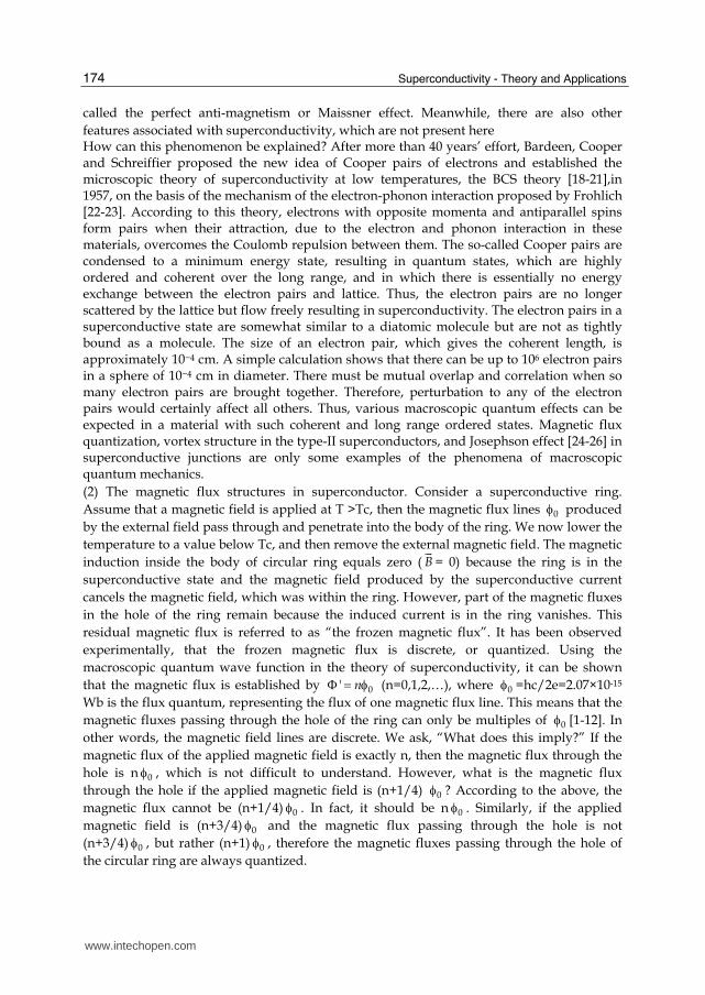
features associated with superconductivity, which are not present here How can this phenomenon be explained? After more than 40 years’ effort, Bardeen, Cooper and Schreiffier proposed the new idea of Cooper pairs of electrons and established the microscopic theory of superconductivity at low temperatures, the BCS theory [18-21],in 1957, on the basis of the mechanism of the electron-phonon interaction proposed by Frohlich [22-23]. According to this theory, electrons with opposite momenta and antiparallel spins form pairs when their attraction, due to the electron and phonon interaction in these materials, overcomes the Coulomb repulsion between them. The so-called Cooper pairs are condensed to a minimum energy state, resulting in quantum states, which are highly ordered and coherent over the long range, and in which there is essentially no energy exchange between the electron pairs and lattice. Thus, the electron pairs are no longer scattered by the lattice but flow freely resulting in superconductivity. The electron pairs in a superconductive state are somewhat similar to a diatomic molecule but are not as tightly bound as a molecule. The size of an electron pair, which gives the coherent length, is approximately 10−4 cm. A simple calculation shows that there can be up to 106 electron pairs in a sphere of 10−4 cm in diameter. There must be mutual overlap and correlation when so many electron pairs are brought together. Therefore, perturbation to any of the electron pairs would certainly affect all others. Thus, various macroscopic quantum effects can be expected in a material with such coherent and long range ordered states. Magnetic flux quantization, vortex structure in the type-II superconductors, and Josephson effect [24-26] in superconductive junctions are only some examples of the phenomena of macroscopic quantum mechanics.

(2) The magnetic flux structures in superconductor. Consider a superconductive ring.

Assume that a magnetic field is applied at T >Tc, then the magnetic flux lines 0 produced

by the external field pass through and penetrate into the body of the ring. We now lower the

temperature to a value below Tc, and then remove the external magnetic field. The magnetic

induction inside the body of circular ring equals zero ( B

= 0) because the ring is in the

superconductive state and the magnetic field produced by the superconductive current

cancels the magnetic field, which was within the ring. However, part of the magnetic fluxes

in the hole of the ring remain because the induced current is in the ring vanishes. This

residual magnetic flux is referred to as “the frozen magnetic flux”. It has been observed

experimentally, that the frozen magnetic flux is discrete, or quantized. Using the

macroscopic quantum wave function in the theory of superconductivity, it can be shown

that the magnetic flux is established by 0' n (n=0,1,2,…), where 0 =hc/2e=2.07×10-15

Wb is the flux quantum, representing the flux of one magnetic flux line. This means that the

magnetic fluxes passing through the hole of the ring can only be multiples of 0 [1-12]. In

other words, the magnetic field lines are discrete. We ask, “What does this imply?” If the

magnetic flux of the applied magnetic field is exactly n, then the magnetic flux through the

hole is n 0 , which is not difficult to understand. However, what is the magnetic flux

through the hole if the applied magnetic field is (n+1/4) 0 ? According to the above, the

magnetic flux cannot be (n+1/4) 0 . In fact, it should be n 0 . Similarly, if the applied

magnetic field is (n+3/4) 0 and the magnetic flux passing through the hole is not

(n+3/4) 0 , but rather (n+1) 0 , therefore the magnetic fluxes passing through the hole of

the circular ring are always quantized.

www.intechopen.com

Properties of Macroscopic Quantum Effects and Dynamic Natures of Electrons in Superconductors

175

An experiment conducted in 1961 surely proves this to be so, indicating that the

magnetic flux does exhibit discrete or quantized characteristics on a macroscopic scale.

The above experiment was the first demonstration of the macroscopic quantum effect.

Based on quantization of the magnetic flux, we can build a “quantum magnetometer”

which can be used to measure weak magnetic fields with a sensitivity of 3×10-7 Oersted.

A slight modification of this device would allow us to measure electric current as low as

2.5×10-9 A.

(3) Quantization of magnetic-flux lines in type-II superconductors. The superconductors

discussed above are referred to as type-I superconductors. This type of superconductor

exhibits a perfect Maissner effect when the external applied field is higher than a critical

magnetic value cH

. There exists other types of materials such as the NbTi alloy and Nb3Sn

compounds in which the magnetic field partially penetrates inside the material when the

external field H

is greater than the lower critical magnetic field 1cH

, but less than the

upper critical field 2cH

[1-7]. This kind of superconductor is classified as type-II

superconductors and is characterized by a Ginzburg-Landau parameter greater than 1/2.

Studies using the Bitter method showed that the penetration of a magnetic field results in

some small regions changing from superconductive to normal state. These small regions in

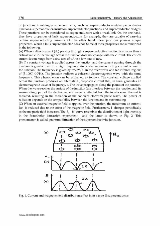
normal state are of cylindrical shape and regularly arranged in the superconductor, as

shown in Fig.1. Each cylindrical region is called a vortex (or magnetic field line)[1-12]. The

vortex lines are similar to the vortex structure formed in a turbulent flow of fluid. Both

theoretical analysis and experimental measurements have shown that the magnetic flux

associated with one vortex is exactly equal to one magnetic flux quantum 0 , when the

applied field 1cH H , the magnetic field penetrates into the superconductor in the form of

vortex lines, increased one by one. For an ideal type-II superconductor, stable vortices are

distributed in triagonal pattern, and the superconducting current and magnetic field

distributions are also shown in Fig. 1. For other, non-ideal type-II superconductors, the

triagonal pattern of distribution can be also observed in small local regions, even though its

overall distribution is disordered. It is evident that the vortex-line structure is quantized and

this has been verified by many experiments and can be considered a result of the

quantization of magnetic flux. Furthermore, it is possible to determine the energy of each

vortex line and the interaction energy between the vortex lines. Parallel magnetic field lines

are found to repel each other while anti-parallel magnetic lines attract each other. (4) The Josephson phenomena in superconductivity junctions [24-26]. As it is known in quantum mechanics, microscopic particles, such as electrons, have a wave property and that can penetrate through a potential barrier. For example, if two pieces of metal are separated by an insulator of width of tens of angstroms, an electron can tunnel through the insulator and travel from one metal to the other. If voltage is applied across the insulator, a tunnel current can be produced. This phenomenon is referred to as a tunneling effect. If two superconductors replace the two pieces of metal in the above experiment, a tunneling

current can also occur when the thickness of the dielectric is reduced to about 300

A . However, this effect is fundamentally different from the tunneling effect discussed above in quantum mechanics and is referred to as the Josephson effect. Evidently, this is due to the long-range coherent effect of the superconductive electron pairs. Experimentally, it was demonstrated that such an effect could be produced via many types

www.intechopen.com


176

of junctions involving a superconductor, such as superconductor-metal-superconductor junctions, superconductor-insulator- superconductor junctions, and superconductor bridges. These junctions can be considered as superconductors with a weak link. On the one hand, they have properties of bulk superconductors, for example, they are capable of carrying certain superconducting currents. On the other hand, these junctions possess unique properties, which a bulk superconductor does not. Some of these properties are summarized in the following. (A) When a direct current (dc) passing through a superconductive junction is smaller than a critical value Ic, the voltage across the junction does not change with the current. The critical current Ic can range from a few tens of μA to a few tens of mA. (B) If a constant voltage is applied across the junction and the current passing through the junction is greater than Ic, a high frequency sinusoidal superconducting current occurs in the junction. The frequency is given by υ=2eV/h, in the microwave and far-infrared regions of (5-1000)×109Hz. The junction radiates a coherent electromagnetic wave with the same frequency. This phenomenon can be explained as follows: The constant voltage applied across the junction produces an alternating Josephson current that, in turn, generates an electromagnetic wave of frequency, υ. The wave propagates along the planes of the junction. When the wave reaches the surface of the junction (the interface between the junction and its surrounding), part of the electromagnetic wave is reflected from the interface and the rest is radiated, resulting in the radiation of the coherent electromagnetic wave. The power of radiation depends on the compatibility between the junction and its surrounding.

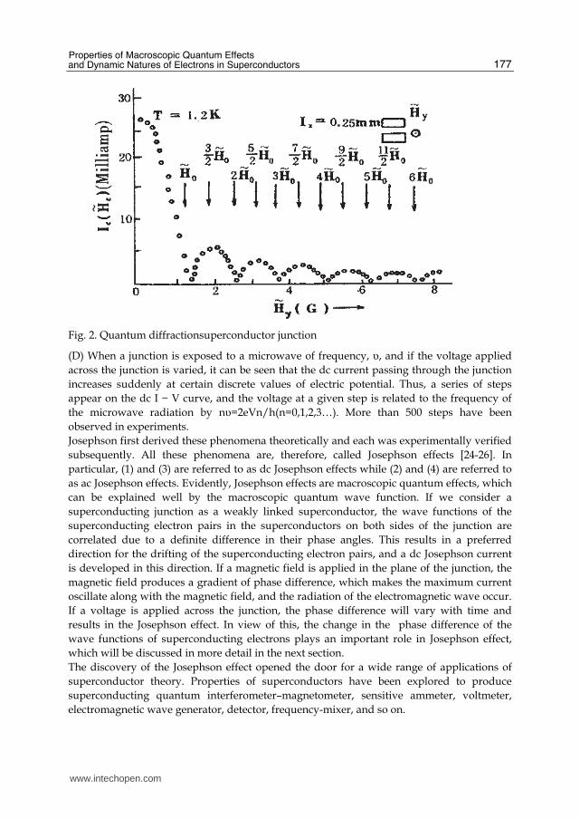
(C) When an external magnetic field is applied over the junction, the maximum dc current,

Ice , is reduced due to the effect of the magnetic field. Furthermore, Ic changes periodically

as the magnetic field increases. The cI H curve resembles the distribution of light intensity

in the Fraunhofer diffraction experiment , and the latter is shown in Fig. 2. This

phenomenon is called quantum diffraction of the superconductivity junction.

Fig. 1. Current and magnetic field distributionseffect in in a type-II superconductor.

www.intechopen.com


177

Fig. 2. Quantum diffractionsuperconductor junction

(D) When a junction is exposed to a microwave of frequency, υ, and if the voltage applied

across the junction is varied, it can be seen that the dc current passing through the junction

increases suddenly at certain discrete values of electric potential. Thus, a series of steps

appear on the dc I − V curve, and the voltage at a given step is related to the frequency of

the microwave radiation by nυ=2eVn/h(n=0,1,2,3…). More than 500 steps have been

observed in experiments.

Josephson first derived these phenomena theoretically and each was experimentally verified

subsequently. All these phenomena are, therefore, called Josephson effects [24-26]. In

particular, (1) and (3) are referred to as dc Josephson effects while (2) and (4) are referred to

as ac Josephson effects. Evidently, Josephson effects are macroscopic quantum effects, which

can be explained well by the macroscopic quantum wave function. If we consider a

superconducting junction as a weakly linked superconductor, the wave functions of the

superconducting electron pairs in the superconductors on both sides of the junction are

correlated due to a definite difference in their phase angles. This results in a preferred

direction for the drifting of the superconducting electron pairs, and a dc Josephson current

is developed in this direction. If a magnetic field is applied in the plane of the junction, the

magnetic field produces a gradient of phase difference, which makes the maximum current

oscillate along with the magnetic field, and the radiation of the electromagnetic wave occur.

If a voltage is applied across the junction, the phase difference will vary with time and

results in the Josephson effect. In view of this, the change in the phase difference of the

wave functions of superconducting electrons plays an important role in Josephson effect,

which will be discussed in more detail in the next section.

The discovery of the Josephson effect opened the door for a wide range of applications of

superconductor theory. Properties of superconductors have been explored to produce

superconducting quantum interferometer–magnetometer, sensitive ammeter, voltmeter,

electromagnetic wave generator, detector, frequency-mixer, and so on.

www.intechopen.com


178

3. The properties of boson condensation and spontaneous coherence of macroscopic quantum effects

3.1 A nonlinear theoretical model of theoretical description of macroscopic quantum effects

From the above studies we know that the macroscopic quantum effect is obviously different

from the microscopic quantum effect, the former having been observed for physical

quantities, such as, resistance, magnetic flux, vortex line, and voltage, etc.

In the latter, the physical quantities, depicting microscopic particles, such as energy,

momentum, and angular momentum, are quantized. Thus it is reasonable to believe that the

fundamental nature and the rules governing these effects are different.

We know that the microscopic quantum effect is described by quantum mechanics.

However, the question remains relative to the definition of what are the mechanisms of

macroscopic quantum effects? How can these effects be properly described?

What are the states of microscopic particles in the systems occurring related to macroscopic

quantum effects? In other words, what are the earth essences and the nature of macroscopic

quantum states? These questions apparently need to be addressed.

We know that materials are composed of a great number of microscopic particles, such as atoms, electrons, nuclei, and so on, which exhibit quantum features. We can then infer, or assume, that the macroscopic quantum effect results from the collective motion and excitation of these particles under certain conditions such as, extremely low temperatures, high pressure or high density among others. Under such conditions, a huge number of microscopic particles pair with each other condense in low-energy state, resulting in a highly ordered and long-range coherent. In such a highly ordered state, the collective motion of a large number of particles is the same as the motion of “single particles”, and since the latter is quantized, the collective motion of the many particle system gives rise to a macroscopic quantum effect. Thus, the condensation of the particles and their coherent state play an essential role in the macroscopic quantum effect.

What is the concept of condensation? On a macroscopic scale, the process of transforming gas into liquid, as well as that of changing vapor into water, is called condensation. This, however, represents a change in the state of molecular positions, and is referred to as a condensation of positions. The phase transition from a gaseous state to a liquid state is a first order transition in which the volume of the system changes and the latent heat is produced, but the thermodynamic quantities of the systems are continuous and have no singularities. The word condensation, in the context of macroscopic quantum effects has its’ special meaning. The condensation concept being discussed here is similar to the phase transition from gas to liquid, in the sense that the pressure depends only on temperature, but not on the volume noted during the process, thus, it is essentially different from the above, first-order phase transition. Therefore, it is fundamentally different from the first-order phase transition such as that from vapor to water. It is not the condensation of particles into a high-density material in normal space. On the contrary, it is the condensation of particles to a single energy state or to a low energy state with a constant or zero momentum. It is thus also called a condensation of momentum. This differs from a first-order phase transition and theoretically it should be classified as a third order phase transition, even though it is really a second order phase transition, because it is related to the discontinuity of the third derivative of a thermodynamic function. Discontinuities can be clearly observed in measured specific heat, magnetic susceptibility of certain systems when condensation

www.intechopen.com


179

occurs. The phenomenon results from a spontaneous breaking of symmetries of the system due to nonlinear interaction within the system under some special conditions such as, extremely low temperatures and high pressures. Different systems have different critical temperatures of condensation. For example, the condensation temperature of a superconductor is its critical temperature cT , and from previous discussions[27-32]. From the above discussions on the properties of superconductors, and others we know that,

even though the microscopic particles involved can be either Bosons or Fermions, those

being actually condensed, are either Bosons or quasi-Bosons, since Fermions are bound as

pairs. For this reason, the condensation is referred to as Bose-Einstein condensation[33-36]

since Bosons obey the Bose-Einstein statistics. Properties of Bosons are different from those

of Fermions as they do not follow the Pauli exclusion principle, and there is no limit to the

number of particles occupying the same energy levels. At finite temperatures, Bosons can

distribute in many energy states and each state can be occupied by one or more particles,

and some states may not be occupied at all. Due to the statistical attractions between Bosons

in the phase space (consisting of generalized coordinates and momentum), groups of Bosons

tend to occupy one quantum energy state under certain conditions. Then when the

temperature of the system falls below a critical value, the majority or all Bosons condense to

the same energy level (e.g. the ground state), resulting in a Bose condensation and a series of

interesting macroscopic quantum effects. Different macroscopic quantum phenomena are

observed because of differences in the fundamental properties of the constituting particles

and their interactions in different systems.

In the highly ordered state of the phenomena, the behavior of each condensed particle is

closely related to the properties of the systems. In this case, the wave function ief or ie of the macroscopic state[33-35], is also the wave function of an individual

condensed particle. The macroscopic wave function is also called the order parameter of the

condensed state. This term was used to describe the superconductive states in the study of

these macroscopic quantum effects. The essential features and fundamental properties of

macroscopic quantum effect are given by the macroscopic wave function and it can be

further shown that the macroscopic quantum states, such as the superconductive states are

coherent and are Bose condensed states formed through second-order phase transitions after

the symmetry of the system is broken due to nonlinear interaction in the system.

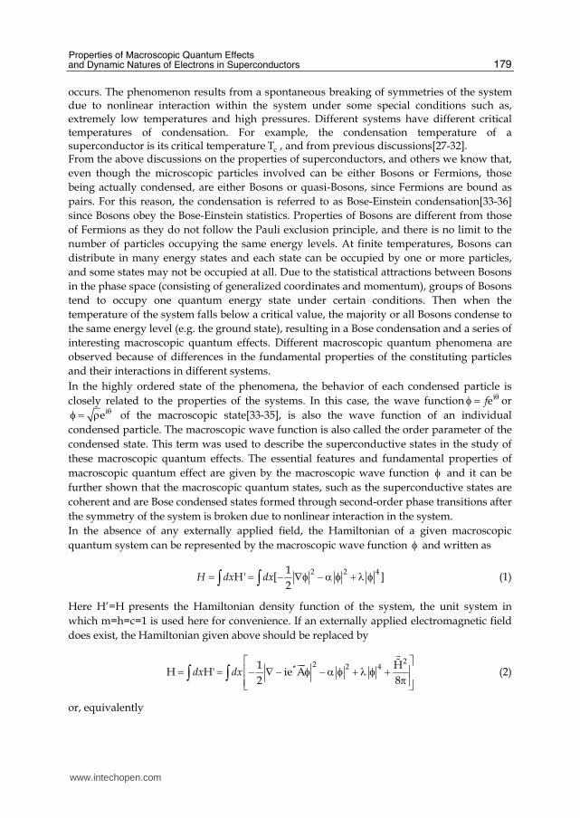
In the absence of any externally applied field, the Hamiltonian of a given macroscopic

quantum system can be represented by the macroscopic wave function and written as

2 2 41

H' [ ]2

H dx dx (1)

Here H’=H presents the Hamiltonian density function of the system, the unit system in

which m=h=c=1 is used here for convenience. If an externally applied electromagnetic field

does exist, the Hamiltonian given above should be replaced by

22 2 4*1 H

H H' ie A2 8

dx dx

(2)

or, equivalently

www.intechopen.com


180

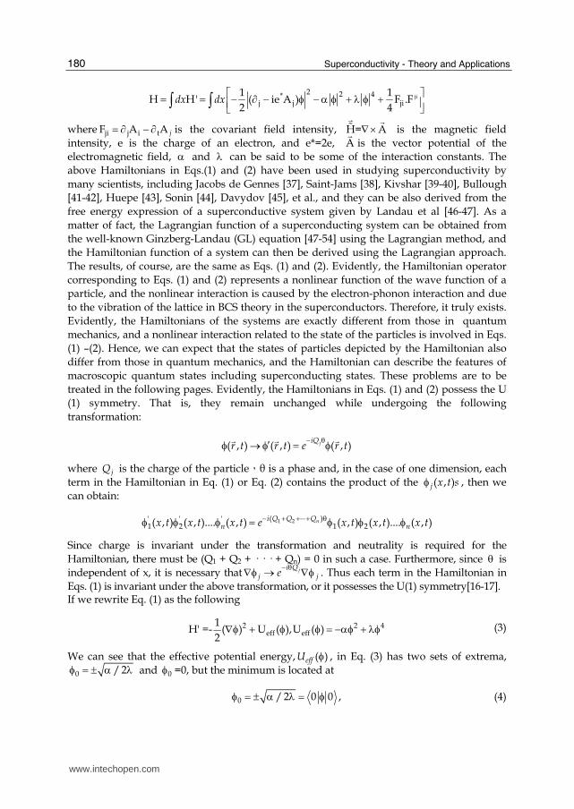
ji2 2 4*

j j ji

1 1H H' ( ie A ) F .F

2 4dx dx

where ji j i tF A A j is the covariant field intensity, H= A is the magnetic field

intensity, e is the charge of an electron, and e*=2e, A

is the vector potential of the

electromagnetic field, and can be said to be some of the interaction constants. The

above Hamiltonians in Eqs.(1) and (2) have been used in studying superconductivity by

many scientists, including Jacobs de Gennes [37], Saint-Jams [38], Kivshar [39-40], Bullough

[41-42], Huepe [43], Sonin [44], Davydov [45], et al., and they can be also derived from the

free energy expression of a superconductive system given by Landau et al [46-47]. As a

matter of fact, the Lagrangian function of a superconducting system can be obtained from

the well-known Ginzberg-Landau (GL) equation [47-54] using the Lagrangian method, and

the Hamiltonian function of a system can then be derived using the Lagrangian approach.

The results, of course, are the same as Eqs. (1) and (2). Evidently, the Hamiltonian operator

corresponding to Eqs. (1) and (2) represents a nonlinear function of the wave function of a

particle, and the nonlinear interaction is caused by the electron-phonon interaction and due

to the vibration of the lattice in BCS theory in the superconductors. Therefore, it truly exists.

Evidently, the Hamiltonians of the systems are exactly different from those in quantum

mechanics, and a nonlinear interaction related to the state of the particles is involved in Eqs.

(1) –(2). Hence, we can expect that the states of particles depicted by the Hamiltonian also

differ from those in quantum mechanics, and the Hamiltonian can describe the features of

macroscopic quantum states including superconducting states. These problems are to be

treated in the following pages. Evidently, the Hamiltonians in Eqs. (1) and (2) possess the U

(1) symmetry. That is, they remain unchanged while undergoing the following

transformation:

( , ) ( , ) ( , )jiQr t r t e r t

where jQ is the charge of the particle，θ is a phase and, in the case of one dimension, each

term in the Hamiltonian in Eq. (1) or Eq. (2) contains the product of the ( , )j x t s , then we

can obtain:

1 2( )' ' '1 2 1 2( , ) ( , ).... ( , ) ( , ) ( , ).... ( , )ni Q Q Q

n nx t x t x t e x t x t x t

Since charge is invariant under the transformation and neutrality is required for the

Hamiltonian, there must be (Q1 + Q2 + · · · + Qn) = 0 in such a case. Furthermore, since is

independent of x, it is necessary that ji Qj je

. Thus each term in the Hamiltonian in

Eqs. (1) is invariant under the above transformation, or it possesses the U(1) symmetry[16-17]. If we rewrite Eq. (1) as the following

2 2 4eff eff

1H' =- ( ) U ( ),U ( )

2 (3)

We can see that the effective potential energy, ( )effU , in Eq. (3) has two sets of extrema,

0 / 2 and 0 =0, but the minimum is located at

0 / 2 0 0 , (4)

www.intechopen.com


181

rather than at 0 =0 . This means that the energy at 0 / 2 is lower than that at 0 =0.

Therefore, 0 =0 corresponds to the normal ground state, while 0 / 2 is the ground

state of the macroscopic quantum systems .

In this case the macroscopic quantum state is the stable state of the system. This shows that

the Hamiltonian of a normal state differs from that of the macroscopic quantum state, in

which the two ground states satisfy 0 0 0 0 under the transformation, .

That is, they no longer have the U(1) symmetry. In other words，the symmetry of the

ground states has been destroyed. The reason for this is evidently due to the nonlinear term 4 in the Hamiltonian of the system. Therefore, this phenomenon is referred to as a

spontaneous breakdown of symmetry. According to Landau’s theory of phase transition,

the system undergoes a second-order phase transition in such a case, and the normal ground

state 0 ==0 is changed to the macroscopic quantum ground state 0 / 2 . Proof will

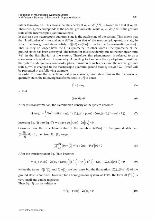
be presented in the following example . In order to make the expectation value in a new ground state zero in the macroscopic quantum state, the following transformation [16-17] is done:

'0 (5)

so that

0 ' 0 =0 (6)

After this transformation, the Hamiltonian density of the system becomes

2 2 2 3 3 4 2 4

0 0 0 0 0 0

1H'( + ) (6 ) 4 (4 2 )

2 (7)

Inserting Eq. (4) into Eq. (7), we have 20 0 04 2 0 .

Consider now the expectation value of the variation H'/ in the ground state, i.e.

'0 0 0

H , then from Eq. (1), we get

2 3'0 0 0 - 2 4 0 0

H (8)

After the transformation Eq. (6), it becomes

2 2 2 3 20 0 0 0 0(4 2 ) 12 0 0 4 0 0 (2 12 ) 0 0 0 (9)

where the terms 30 0 and 0 0 are both zero, but the fluctuation 2012 0 0 of the

ground state is not zero. However, for a homogeneous system, at T=0K, the term 20 0 is

very small and can be neglected. Then Eq. (9) can be written as

2 20 0 0- (4 2 ) 0 (10)

www.intechopen.com


182

Obviously, two sets of solutions, 0 0 , and 0 / 2 , can be obtained from the

above equation, but we can demonstrate that the former is unstable, and that the latter is

stable.

If the displacement is very small, i.e. '0 0 0 0 , then the equation satisfied by the

fluctuation 0 is relative to the normal ground state 0 0 and is

20 02 0 (11)

Its’ solution attenuates exponentially indicating that the ground state, 0 0 is unstable.

On the other hand, the equation satisfied by the fluctuation 0 , relative to the ground

state 0 / 2 is 20 02 0 . Its’ solution, 0 , is an oscillatory function and

thus the macroscopic quantum state ground state 0 / 2 is stable. Further

calculations show that the energy of the macroscopic quantum state ground state is lower

than that of the normal state by 20 / 4 0 .Therefore, the ground state of the

normal phase and that of the macroscopic quantum phase are separated by an energy gap

of 2 /(4 ) so then, at T=0K, all particles can condense to the ground state of the

macroscopic quantum phase rather than filling the ground state of the normal phase. Based on this energy gap, we can conclude that the specific heat of the macroscopic quantum systems has an exponential dependence on the temperature, and the critical

temperature is given by: c pT =1.14 exp[ 1 /(3 / )N(0)] [16-17]. This is a feature of the

second-order phase transition. The results are in agreement with those of the BCS theory of superconductivity.

Therefore, the transition from the state 0 0 to the state 0 / 2 and the

corresponding condensation of particles are second-order phase transitions. This is

obviously the results of a spontaneous breakdown of symmetry due to the nonlinear

interaction, 4 .

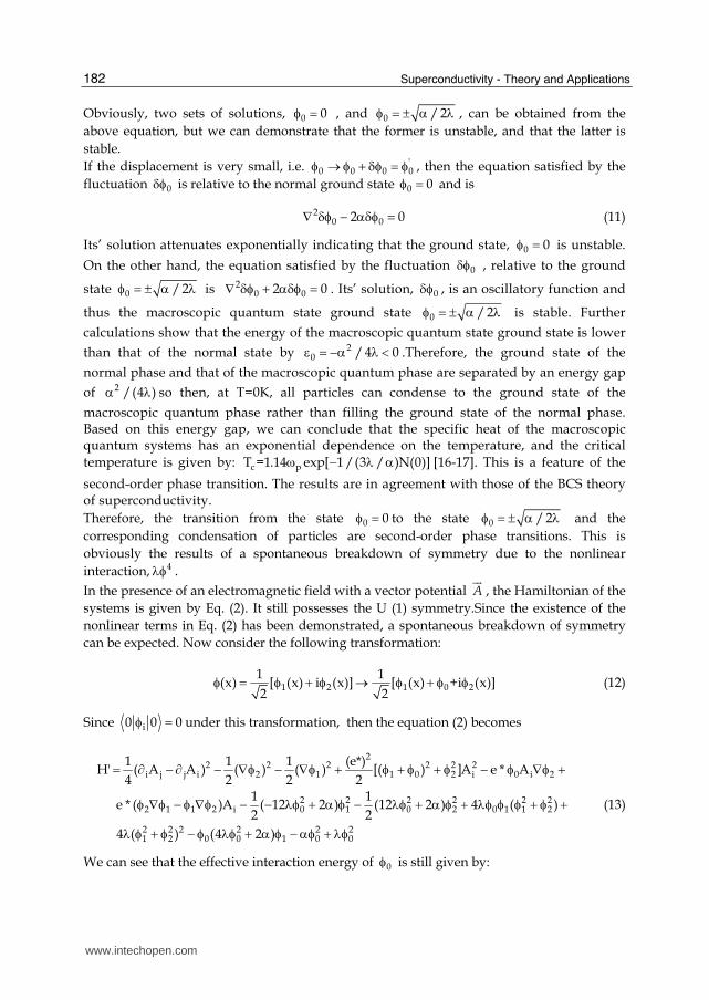
In the presence of an electromagnetic field with a vector potential A

, the Hamiltonian of the

systems is given by Eq. (2). It still possesses the U (1) symmetry.Since the existence of the

nonlinear terms in Eq. (2) has been demonstrated, a spontaneous breakdown of symmetry

can be expected. Now consider the following transformation:

1 2 1 0 2

1 1(x) [ (x) i (x)] [ (x) +i (x)]

2 2 (12)

Since i0 0 0 under this transformation, then the equation (2) becomes

22 2 2 2 2 2

i j j i 2 1 1 0 2 i 0 i 2

2 2 2 2 2 22 1 1 2 i 0 1 0 2 0 1 1 2

2 2 2 2 2 21 2 0 0 1 0 0

1 1 1 (e*)H' ( A A ) ( ) ( ) [( ) ]A e * A

4 2 2 21 1

e * ( )A ( 12 2 ) (12 2 ) 4 ( )2 2

4 ( ) (4 2 )

(13)

We can see that the effective interaction energy of 0 is still given by:

www.intechopen.com


183

2 4eff 0 0 0U ( ) (14)

and is in agreement with that given in Eq. (4). Therefore, using the same argument, we can

conclude that the spontaneous symmetry breakdown and the second-order phase transition

also occur in the system. The system is changed from the ground state of the normal

phase, 0 0 to the ground state 0 / 2 of the condensed phase in such a case. The

above result can also be used to explain the Meissner effect and to determine its critical

temperature in the superconductor. Thus, we can conclude that, regardless of the existence

of any external field macroscopic quantum states, such as the superconducting state, are

formed through a second-order phase transition following a spontaneous symmetry

breakdown due to nonlinear interaction in the systems.

3.2 The features of the coherent state of macroscopic quantum effects

Proof that the macroscopic quantum state described by Eqs. (1) - (2) is a coherent state, using

either the second quantization theory or the solid state quantum field theory is presented in

the following paragraphs and pages.

As discussed above, when '/H =0 from Eq. (1), we have

22 2 4 0 (15)

It is a time-independent nonlinear Schrödinger equation (NLSE), which is similar to the GL

equation. Expanding in terms of the creation and annihilation operators, +bp and bp

.ip xip +

p pp p

1 1(b e b e )

2V

x (16)

where V is the volume of the system. After a spontaneous breakdown of symmetry, 0 , the

ground-state of , for the system is no longer zero, but 0 / 2 . The operation of the

annihilation operator on 0 no longer gives zero, i.e.

p 0b 0 (17)

A new field ' can then be defined according to the transformation Eq. (5), where 0 is

a scalar field and satisfies Eq. (10) in such a case. Evidently, 0 can also be expanded

into

.x .ip ip x+0 p p

p p

1 1( e e )

2V

(18)

The transformation between the fields and ' is obviously a unitary transformation, that

is

' 1 s s

0U U e e (19)

where

www.intechopen.com


184

' ' ' ' ' '0 0S i [ (x , t) (x , t) (x , t) (x , t)]dx (20)

and ' satisfy the following commutation relation

' ' '[ (x , t), (x, t)] i (x )x (21)

From Eq. (6) we now have '00 ' 0 0 . The ground state '

0 of the field ' thus

satisfies

'p 0b 0 (22)

From Eq. (6), we can obtain the following relationship between the annihilation operator ap

of the new field ' and the annihilation operator bp of the field

S Sp p p pa e b e =b (23)

where

. .ip x -ip x*p 0 03/2

p

1[ (x, t)e i (x, t)e ]

(2 )

dx (24)

Therefore, the new ground state '0 and the old ground state 0 are related through

' S0 0e .

Thus we have

' ' 'p 0 p p 0 p 0a (b ) (25)

According to the definition of the coherent state, equation (25) we see that the new ground

state '0 is a coherent state. Because such a coherent state is formed after the spontaneous

breakdown of symmetry of the systems, thus, it is referred to as a spontaneous coherent

state. But when 0 0 , the new ground state is the same as the old state, which is not a

coherent state.The same conclusion can be directly derived from the BCS theory [18-21]. In

the BCS theory, the wave function of the ground state of a superconductor is written as

' + + + +k0 k k k -k 0 k k k-k 0 k-k 0

kkk k

ˆ ˆˆ( a a ) ( b ) ~ 'exp( b ) (26)

where + + +k-k k -k

ˆ ˆ ˆb a a . This equation shows that the superconducting ground state is a

coherent state. Hence, we can conclude that the spontaneous coherent state in

superconductors is formed after the spontaneous breakdown of symmetry. By reconstructing a quasiparticle-operator-free new formulation of the Bogoliubov-Valatin

transformation parameter dependence [55], W. S. Lin et al [56] demonstrated that the BCS

state is not only a coherent state of single-Cooper-pairs, but also the squeezed state of the

double-Cooper- pairs, and reconfirmed thus the coherent feature of BCS superconductive

state.

www.intechopen.com


185

3.3 The Boson condensed features of macroscopic quantum effects We will now employ the method used by Bogoliubov in the study of superfluid liquid helium 4He to prove that the above state is indeed a Bose condensed state. To do that, we rewrite Eq. (16) in the following form [12-17]

ipxp p p - p

p p

1 1( ) ,

2x q e q b b

V

(27)

Since the field describes a Boson, such as the Cooper electron pair in a superconductor

and the Bose condensation can occur in the system, we will apply the following traditional

method in quantum field theory, and consider the following transformation:

p 0 p p 0 p( ) , ( )b N p b N p (28)

where 0N is the number of Bosons in the system and 0 ,if p 0

( )1 , if p=0

p . Substituting Eqs.

(27) and (28) into Eq. (1), we can arrive at the Hamiltonian operator of the system as follows

0 0

0 0

2 2+ +0

0 0 0 p p - p p - p2 20 0 PP0 0

+ + + +p - p p - p p - p0 0

+ + +0 0 pp p - p p p p p

0 0p p p p p

0 0 0 Pp

4 44

2 1

2 2

4 4

2 p

N NNH N

VV V

N N

V

N N

V V

0 02

P

N NO O

V V

(29)

Because the condensed density 0N V must be finite, it is possible that the higher order

terms 00 N V and 200 N V may be neglected. Next we perform the following

canonical transformation

* *p p p p - p p p p p - p,.u c c u d d (30)

where pv and pu are real and satisfy 2 2p p 1u . This introduces another transformation

p p p p -p p p p - p

1

2u u , p p p p - p p p p - p

1

2u u (31)

the following relations can be obtained

p p p p -p, ,H g M p p p p -p,H g M (32)

where

2 2 2 2p p p p p p p p p p p p p p;

2 2 2 2p p p p p p p p p p p p p

2 , M 2

2 , M 2 p

g G u F u F u G u

g G u F u F u G u

(33)

www.intechopen.com


186

while

p p p p p

p p

6 , F 62 2

G , '

p p p pp p

2 , F 22 2

pG (34)

where ' 0

0 p

N=

Vp

.

We will now study two cases to illustrate the concepts.

(A) Let p 0M , then it can be seen from Eq. (32) that +p is the creation operator of

elementary excitation and its energy is given by

2p p p p4 2g (35)

Using this concept, we can obtain the following form from Eqs. (32) and (34)

2 pp

p

11

2

Gu

g

and 2 p

pp

11

2

G

g

(36)

From Eq. (32), we know that +p is not a creation operator of the elementary excitation. Thus,

another transformation must be made

2 2

p p p p p p p, 1B (37)

We can then prove that

[ , ]pB H p pE B (38)

where 2p p pE 12 2p

.

Now, inserting Eqs. (30), (37)-(38) and pM 0 into Eq. (29), and after some reorganization,

we have

0 p p p - p - p p p p - p - pp>0

H U E E B B B B g (39)

where

220 0

p p p p p20 pp p p>00

24 4 4 4 2

2

N NU u

V

2

0 p p p pp>0 p>0

2E E g E (40)

Both U and 0E are now independent of the creation and annihilation operators of the

Bosons. 0U E gives the energy of the ground state. 0N can be determined from the

condition, 0

0

0U E

N

, which gives

www.intechopen.com


187

20 00 0

1

4 2

N

V

(41)

This is the condensed density of the ground state 0 . From Eqs. (36), (37) and (40), thus we can arrive at:

2 2p p p p, Eg (42)

These correspond to the energy spectra of p and pB ,respectively, and they are similar to

the energy spectra of the Cooper pair and phonon in the BCS theory. Substituting Eq. (42) into Eq. (36), thus we now have:

2 2p p2 2

p p2 2p p p p

2 - 21 1u 1+ , -1+

2 22 - e 2

(43)

(B) In the case of Mp=0, a similar approach can be used to arrive at the energy spectrum corresponding to +

p as 2p pE , while that corresponding to +

p p p p -pA is 2

p pg , where

2 2p p2 2

p p2 2

p p p p

2 21 1u 1+ , -1+

2 22 2

(44)

Based on experiments in quantum statistical physics, we know that the occupation number of the level with an energy of p , for a system in thermal equilibrium at temperature T( 0) is shown as:

p B

p p p K T

1N b b

e 1

(45)

where denotes Gibbs average, defined as B

B

K T

K T

SP e

SP e

, here SP denotes the

trace in a Gibbs statistical description. At low temperatures, or T 0 K , the majority of the

Bosons or Cooper pairs in a superconductor condense to the ground state with p 0 .

Therefore 0 0 0b b N , where 0N is the total number of Bosons or Cooper pairs in the

system and 0N 1 , i.e. 0 0b b 1 b b .

As can be seen from Eqs. (27) and (28), the number of particles is extremely large when they lie in condensed state, that is to say:

0 p=0 0 0

0

1b b

2 V

(46)

Because 0 0 0 and 0 0 0 , 0b and 0b can be taken to be 0N . The average value of in the ground state then becomes

www.intechopen.com


188

00 0 0

00 0

214

2

NN

V V (47)

Substituting Eq. (41) into Eq. (47), we can see that:

0 2 or

0 2

which is the ground state of the condensed phase, or the superconducting phase, that we

have known. Thus, the density of states, 0N V , of the condensed phase or the

superconducting phase formed after the Bose condensation coincides with the average value

of the Boson’s (or Copper pair’s) field in the ground state. We can then conclude from the

above investigation shown in Eqs. (1) - (2) that the macroscopic quantum state or the

superconducting ground state formed after the spontaneous symmetry breakdown is indeed

a Bose-Einstein condensed state. This clearly shows the essences of the nonlinear properties

of the result of macroscopic quantum effects. In the last few decades, the Bose-Einstein condensation has been observed in a series of

remarkable experiments using weakly interacting atomic gases, such as vapors of rubidium,

sodium lithium, or hydrogen. Its’ formation and properties have been extensively studied.

These studies show that the Bose-Einstein condensation is a nonlinear phenomenon,

analogous to nonlinear optics, and that the state is coherent, and can be described by the

following NLSE or the Gross-Pitaerskii equation [57-59]:

23

2i V x

t' x'

(48)

where t =t , x =x 2m . This equation was used to discuss the realization of the Bose-

Einstein condensation in the d 1 dimensions (d 1,2,3) by H. K. Bullough et.al [41-42].

Too, Elyutin et al [60-61]. gave the corresponding Hamiltonian density of a condensate

system as follows:

2

2 41' ( ')

' 2H V x

x

(49)

where H’=H, the nonlinear parameters of are defined as 21 02 /Naa a , with N being

the number of particles trapped in the condensed state, a is the ground state scattering

length, a0 and a1 are the transverse (y, z) and the longitudinal (x) condensate sizes (without

self-interaction) respectively, (Integrations over y and z have been carried out in obtaining

the above equation). is positive for condensation with self-attraction (negative scattering

length).The coherent regime was observed in Bose-Einstein condensation in lithium. The

specific form of the trapping potential V (x’) depends on the details of the experimental

setup. Work on Bose-Einstein condensation based on the above model Hamiltonian were

carried out and are reported by C. F. Barenghi et al [31]. It is not surprising to see that Eq. (48) is exactly the same as Eq. (15), corresponding to the Hamiltonian density in Eq. (49) and, where used in this study is naturally the same as Eq. (1). This prediction confirms the correctness of the above theory for Bose-Einstein

www.intechopen.com


189

condensation. As a matter of fact, immediately after the first experimental observation of this condensation phenomenon, it was realized that the coherent dynamics of the condensed macroscopic wave function could lead to the formation of nonlinear solitary waves. For example, self-localized bright, dark and vortex solitons, formed by increased (bright) or decreased (dark or vortex) probability density respectively, were experimentally observed, particularly for the vortex solution which has the same form as the vortex lines found in type II-superconductors and superfluids. These experimental results were in concordance with the results of the above theory. In the following sections of this text we will study the soliton motions of quasiparticles in macroscopic quantum systems, superconductors. We will see that the dynamic equations in macroscopic quantum systems do have such soliton solutions.

3.4 Differences of macroscopic quantum effects from the microscopic quantum effects

From the above discussion we may clearly understand the nature and characteristics of macroscopic quantum systems. It would be interesting to compare the macroscopic quantum effects and microscopic quantum effects. Here we give a summary of the main differences between them. 1. Concerning the origins of these quantum effects; the microscopic quantum effect is

produced when microscopic particles, which have only a wave feature are confined in a finite space, or are constituted as matter, while the macroscopic quantum effect is due to the collective motion of the microscopic particles in systems with nonlinear interaction. It occurs through second-order phase transition following the spontaneous breakdown of symmetry of the systems.

2. From the point-of-view of their characteristics, the microscopic quantum effect is characterized by quantization of physical quantities, such as energy, momentum, angular momentum, etc. wherein the microscopic particles remain constant. On the other hand, the macroscopic quantum effect is represented by discontinuities in macroscopic quantities, such as, the resistance, magnetic flux, vortex lines, voltage, etc. The macroscopic quantum effects can be directly observed in experiments on the macroscopic scale, while the microscopic quantum effects can only be inferred from other effects related to them.

3. The macroscopic quantum state is a condensed and coherent state, but the microscopic quantum effect occurs in determinant quantization conditions, which are different for the Bosons and Fermions. But, so far, only the Bosons or combinations of Fermions are found in macroscopic quantum effects.

4. The microscopic quantum effect is a linear effect, in which the microscopic particles and are in an expanded state, their motions being described by linear differential equations such as the Schrödinger equation, the Dirac equation, and the Klein- Gordon equations.

On the other hand, the macroscopic quantum effect is caused by the nonlinear interactions, and the motions of the particles are described by nonlinear partial differential equations such as the nonlinear Schrödinger equation (17). Thus, we can conclude that the macroscopic quantum effects are, in essence, a nonlinear

quantum phenomenon. Because its’ fundamental nature and characteristics are different

from those of the microscopic quantum effects, it may be said that the effects should be

depicted by a new nonlinear quantum theory, instead of quantum mechanics.

www.intechopen.com


190

4. The nonlinear dynamic natures of electrons in superconductors

4.1 The dynamic equations of electrons in superconductors

It is quite clear from the above section that the superconductivity of material is a kind of

nonlinear quantum effect formed after the breakdown of the symmetry of the system due to

the electron-phonon interaction, which is a nonlinear interaction.

In this section we discuss the properties of motion of superconductive electrons in superconductors and the relation of the solutions of dynamic equations in relation to the above macroscopic quantum effects on it. The study presented shows that the superconductive electrons move in the form of a soliton, which can result in a series of macroscopic quantum effects in the superconductors. Therefore, the properties and motions of the quasiparticles are important for understanding the essences and rule of superconductivity and macroscopic quantum effects. As it is known, in the superconductor the states of the electrons are often represented by a

macroscopic wave function,

( , )0( , ) ( , ) i r tr t f r t e

, or ie ,

as mentioned above, where 20 / 2 . Landau et al [45,46] used the wave function to give

the free energy density function, f, of a superconducting system, which is represented by

2

2 2 4

2s nf f

m

(50)

in the absence of any external field. If the system is subjected to an electromagnetic field

specified by a vector potential A

, the free energy density of the system is of the form:

22

2 4 2* 1( ) H

2 8s n

ief f A

m c

(51)

where e*=2e , H= A , and are some interactional constants related to the features of

superconductor, m is the mass of electron, e* is the charge of superconductive electron, c is

the velocity of light, h is Planck constant, / 2h , fn is the free energy of normal state.

The free energy of the system is 3s sF f d x . In terms of the conventional

field, jjl j l lF A A , (j, l=1, 2, 3), the term 2H /8

can be written as / 4jljlF F . Equations

(50) - (51) show the nonlinear features of the free energy of the systems because it is the

nonlinear function of the wave function of the particles, ( , )r t . Thus we can predict that the

superconductive electrons have many new properties relative to the normal electrons. From

/ 0sF we get

2

2 32 02m

(52)

and

2

2 3*( ) 2 0

2

ieA

m c

(53)

www.intechopen.com


191

in the absence and presence of an external fields respectively, and

2* *

( * *)2

e eJ A

mi mc

(54)

Equations (52) - (54) are just well-known the Ginzburg-Landau (GL) equation [48-54] in a steady state, and only a time-independent Schrödinger equation. Here, Eq. (52) is the GL equation in the absence of external fields. It is the same as Eq. (15), which was obtained from Eq. (1). Equation (54) can also be obtained from Eq. (2). Therefore, Eqs. (1)-(2) are the Hamiltonians corresponding to the free energy in Eqs. (50)- (51).

From equations (52) - (53) we clearly see that superconductors are nonlinear systems.

Ginzburg-Landau equations are the fundamental equations of the superconductors

describing the motion of the superconductive electrons, in which there is the nonlinear term

of 32 . However, the equations contain two unknown functions and A

which make

them extremely difficult to resolve.

4.2 The dynamic properties of electrons in steady superconductors

We first study the properties of motion of superconductive electrons in the case of no external field. Then, we consider only a one-dimensional pure superconductor [62-63], where

2 2

0 ( , ), ' ( ) / 2 , / '( )x t T m x x T

(55)

and where '( )T is the coherent length of the superconductor, which depends on

temperature. For a uniform superconductor, 20'( ) 0.94 [ /( )]c cT T T T , where cT is the

critical temperature and 0 is the coherent length of superconductive electrons at T=0. In

boundary conditions of (x=0)=1 , and (x ) =0, from Eqs. (52) and (54) we find

easily its solution as:

02 sec'( )

x xh

T

or

00

2sec [ ] sec [ ( )]

'( )

x x mh h x x

T

(56)

This is a well-known wave packet-type soliton solution. It can be used to represent the

bright soliton occurred in the Bose-Einstein condensate found by Perez-Garcia et. al. [64]. If

the signs of and in Eq. (52) are reversed, we then get a kink-soliton solution under the

boundary conditions of (x=0)=0, (x )= 1,

1/2 2 1/20( / 2 ) tanh{[ ( / ] }m x x (57)

The energy of the soliton, (56), is given by

www.intechopen.com


192

2 3/2

2 2 41

4( )

2 3 2so

dE dx

m dx m

(58)

We assume here that the lattice constant, r0=1. The above soliton energy can be compared

with the ground state energy of the superconducting state, Eground= 2 /4 . Their

difference is 3/21 ground

16/ 2 0

3 2soE E

m

. This indicates clearly that the soliton

is not in the ground state, but in an excited state of the system, therefore, the soliton is a

quasiparticle.

From the above discussion, we can see that, in the absence of external fields, the

superconductive electrons move in the form of solitons in a uniform system. These solitons

are formed by a nonlinear interaction among the superconductive electrons which

suppresses the dispersive behavior of electrons. A soliton can carry a certain amount of

energy while moving in superconductors. It can be demonstrated that these soliton states

are very stable.

4.3 The features of motion of superconductive electrons in an electromagnetic field and its relation to macroscopic quantum effects

We now consider the motion of superconductive electrons in the presence of an

electromagnetic field A

; its equation of motion is denoted by Eqs. (53)-(54)．Assuming now

that the field A

satisfies the London gauge 0A [65], and that the substitution of

( )0( , ) ( , ) i rr t r t e

into Eqs. (53) and (54) yields [66-67]:

2

20* *= ( )

e eJ A

m c

(59)

and

2 2 2 202

* 2[( ) ] ( 2 ) 0

e m

c A

(60)

For bulk superconductors, J is a constant (permanent current) for a certain value of A

, and

it thus can be taken as a parameter. Let 2 2 2 2 2 40/ ( *)B m J e , 2 22 / 'b m , from Eqs.

(59) and (60), we can obtain [66-67]:

2 20

*( )

*

e Jm

c e A

(61)

2 2

2 4eff eff2 2

1 1 ( ), ( )

2 42

d d BU U b b

ddx

(62)

where Ueff is the effective potential of the superconductive electron in this case and it is schematically shown in Fig. 2. Comparing this case with that in the absence of external fields, we found that the equations have the same form and the electromagnetic field changes only the effective potential of the superconductive electron. When 0A

, the

www.intechopen.com


193

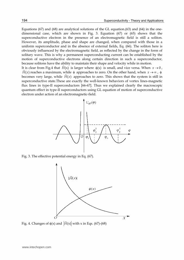
effective potential well is characterized by double wells. In the presence of an electromagnetic field, there are still two minima in the effective potential, corresponding to the two ground states of the superconductor in this condition. This shows that the spontaneous breakdown of symmetry still occurs in the superconductor, thus the superconductive electrons also move in the form of solitons. To obtain the soliton solution, we integrate Eq. (62) and can get:

1

eff2[ ( )

dx

E U

(63)

Where E is a constant of integration which is equivalent to the energy, the lower limit of the integral, 1 , is determined by the value of at x=0, i.e. eff 0 eff 1( ) ( )E U U . Introduce

the following dimensionless quantities 2 ,u 2

2 2

4, 2

2 ( *)

b J mE d

e

, and equation (63) can

be written as the following upon performing the transformation u→u,

1 3 2 2

22 3 2

u

u

dubx

u u u d

(64)

It can be seen from Fig. 3 that the denominator in the integrand in Eq. (64) approaches zero

linearly when u=u1=21 , but approaches zero gradually when u=u2=

20 . Thus we give [66-67]

2 2 20 1

1 1( ) ( ) sec tan

2 2u x x u g h gbx u g h gbx

(65)

where g= u0u1 and satisfies

2 2(2 ) (1 ) 27g g d , 0 12 =2u u , 2

0 0 12 2u u u , 2 21 0 =2u u d (66)

It can be seen from Eq. (65) that for a large part of sample, u1 is very small and may be neglected; the solution u is very close to u0. We then get from Eq. (65) that

0

1( ) tan

2x h gbx

(67)

Substituting the above into Eq. (61), the electromagnetic field A

in the superconductors can

be obtained

2 2 2 2 2 20 0 0

1 1 cot

* 2 *(e*) ( *)

Jmc c Jmc cA h gbx

e ee

For a large portion of the superconductor, the phase change is very small. Using H A

the magnetic field can be determined and is given by [66-67]

32 2 2

0 0

2 1 1[cot cot ]

2 2( *)

Jmc gbH h gbx h gbx

e

(68)

www.intechopen.com


194

Equations (67) and (68) are analytical solutions of the GL equation.(63) and (64) in the one-dimensional case, which are shown in Fig. 3. Equation (67) or (65) shows that the superconductive electron in the presence of an electromagnetic field is still a soliton. However, its amplitude, phase and shape are changed, when compared with those in a uniform superconductor and in the absence of external fields, Eq. (66). The soliton here is obviously influenced by the electromagnetic field, as reflected by the change in the form of solitary wave. This is why a permanent superconducting current can be established by the motion of superconductive electrons along certain direction in such a superconductor, because solitons have the ability to maintain their shape and velocity while in motion.

It is clear from Fig.4 that (x)H is larger where (x) is small, and vice versa. When 0x ,

( )H x reaches a maximum, while approaches to zero. On the other hand, when x ,

becomes very large, while ( )H x approaches to zero. This shows that the system is still in

superconductive state.These are exactly the well-known behaviors of vortex lines-magnetic

flux lines in type-II superconductors [66-67]. Thus we explained clearly the macroscopic

quantum effect in type-II superconductors using GL equation of motion of superconductive

electron under action of an electromagnetic-field.

Fig. 3. The effective potential energy in Eq. (67).

Fig. 4. Changes of (x) and (x)H with x in Eqs. (67)-(68)

www.intechopen.com


195

Recently, Garadoc-Daries et al. [68], Matthews et al. [69] and Madison et al.[70] observed

vertex solitons in the Boson-Einstein condensates. Tonomure [71] observed experimentally

magnetic vortexes in superconductors. These vortex lines in the type-II-superconductors are

quantized. The macroscopic quantum effects are well described by the nonlinear theory

discussed above, demonstrating the correctness of the theory.

We now proceed to determine the energy of the soliton given by (67). From the earlier

discussion, the energy of the soliton is given by:

2 22 2+ 2 2 4 2 0 0

02 20

21 b= ( ) 1 (1 )

2 2 4 3 2 22 2

bd b B b BE dx

dx

which depends on the interaction between superconductive electrons and electromagnetic

field.

From the above discussion, we understand that for a bulk superconductor, the

superconductive electrons behave as solitons, regardless of the presence of external fields.

Thus, the superconductive electrons are a special type of soliton. Obviously, the solitons are

formed due to the fact that the nonlinear interaction2 suppresses the dispersive effect

of the kinetic energy in Eqs. (52) and (53). They move in the form of solitary wave in the

superconducting state. In the presence of external electromagnetic fields, we demonstrate

theoretically that a permanent superconductive current is established and that the vortex

lines or magnetic flux lines also occur in type-II superconductors.

5. The dynamic properties of electrons in superconductive junctions and its relation to macroscopic quantum effects

5.1 The features of motion of electron in S-N junction and proximity effect

The superconductive junction consists of a superconductor (S) which contacts with a normal

conductor (N), in which the latter can be superconductive. This phenomenon refers to a

proximity effect. This is obviously the result of long- range coherent property of

superconductive electrons. It can be regarded as the penetration of electron pairs from the

superconductor into the normal conductor or a result of diffraction and transmission of

superconductive electron wave. In this phenomenon superconductive electrons can occur in

the normal conductor, but their amplitudes are much small compare to that in the

superconductive region, thus the nonlinear term 2 in GL equations (53)-(54) can be

neglected. Because of these, GL equations in the normal and superconductive regions have

different forms. On the S side of the S-N junction, the GL equation is [72]

2 *

3ie( A) 2 0

2m ch

(69)

while that on the N side of the junction is

2 *ie

( A) ' 02m ch

(70)

Thus, the expression for J

remains the same on both sides.

www.intechopen.com


196

* 2

2* *e (e*)J ( ) A

2mi mc

(71)

In the S region, we have obtained solution of (69) in the previous section, and it is given by (65) or (67) and (68). In the N region, from Eqs. (70)- (71) we can easily obtain

'2 ' 2 2 '

'2 2 2 2i ' 2 2 ' i2 2 i2N 0 0

1( ) 4d sin(2 b x)

2 2

1e ( ) 4d sin(2 b x)e e

2 2

(72)

where '

'2 '2

2m 1b ,

2

22 2

4J m2d ,

(e*) '

'

' 'bE .

2 .

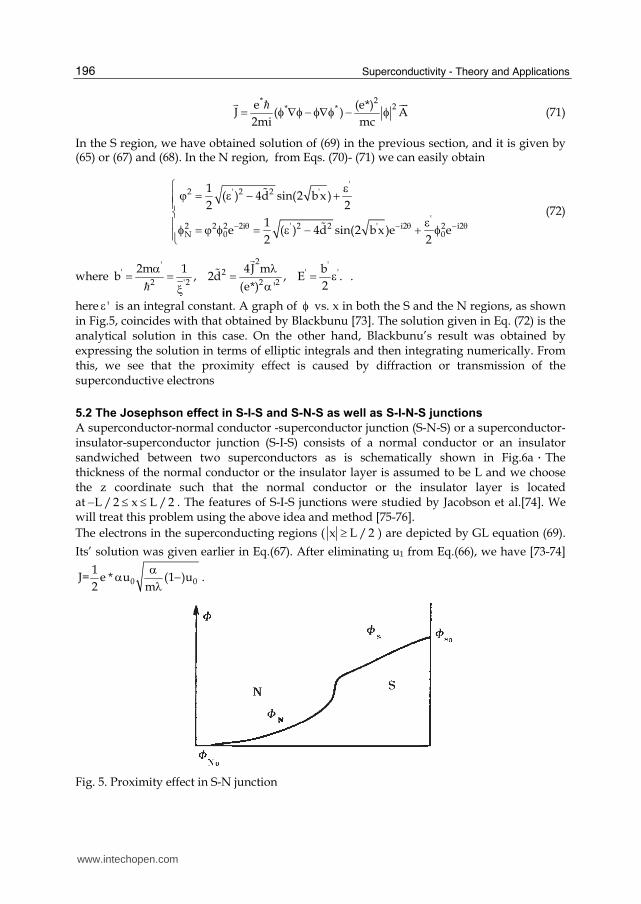
here ' is an integral constant. A graph of vs. x in both the S and the N regions, as shown in Fig.5, coincides with that obtained by Blackbunu [73]. The solution given in Eq. (72) is the analytical solution in this case. On the other hand, Blackbunu’s result was obtained by expressing the solution in terms of elliptic integrals and then integrating numerically. From this, we see that the proximity effect is caused by diffraction or transmission of the superconductive electrons

5.2 The Josephson effect in S-I-S and S-N-S as well as S-I-N-S junctions

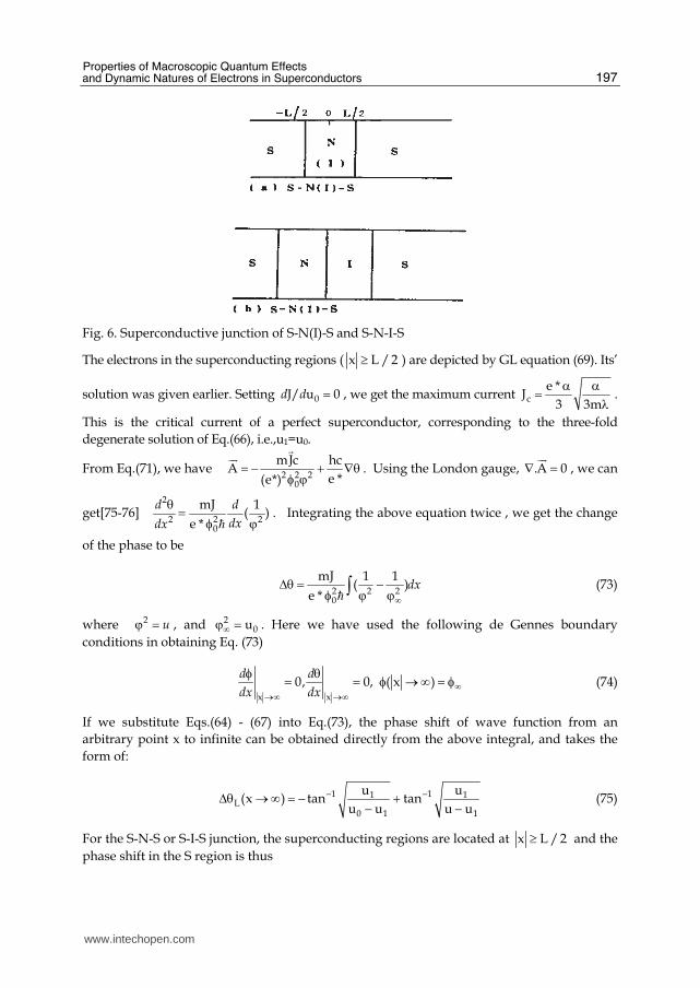
A superconductor-normal conductor -superconductor junction (S-N-S) or a superconductor-insulator-superconductor junction (S-I-S) consists of a normal conductor or an insulator sandwiched between two superconductors as is schematically shown in Fig.6a．The thickness of the normal conductor or the insulator layer is assumed to be L and we choose the z coordinate such that the normal conductor or the insulator layer is located at L / 2 x L / 2 . The features of S-I-S junctions were studied by Jacobson et al.[74]. We will treat this problem using the above idea and method [75-76].

The electrons in the superconducting regions ( x L / 2 ) are depicted by GL equation (69).

Its’ solution was given earlier in Eq.(67). After eliminating u1 from Eq.(66), we have [73-74]

0 0

1J= e * u (1 )u

2 m

.

Fig. 5. Proximity effect in S-N junction

www.intechopen.com


197

Fig. 6. Superconductive junction of S-N(I)-S and S-N-I-S

The electrons in the superconducting regions ( x L / 2 ) are depicted by GL equation (69). Its’

solution was given earlier. Setting 0J/ u 0d d , we get the maximum current c

e *J

3 3m

.

This is the critical current of a perfect superconductor, corresponding to the three-fold

degenerate solution of Eq.(66), i.e.,u1=u0.

From Eq.(71), we have 2 2 2

0

mJc hcA

e *(e*)

. Using the London gauge, .A 0

, we can

get[75-76] 2

2 2 20

mJ 1( )

e *

d d

dxdx

. Integrating the above equation twice , we get the change

of the phase to be

2 2 20

mJ 1 1( )

e *dx

(73)

where 2 u , and 20u . Here we have used the following de Gennes boundary

conditions in obtaining Eq. (73)

x x

0, 0, ( x )d d

dx dx

(74)

If we substitute Eqs.(64) - (67) into Eq.(73), the phase shift of wave function from an

arbitrary point x to infinite can be obtained directly from the above integral, and takes the

form of:

1 11 1L

0 1 1

u u(x ) tan tan

u u u u (75)

For the S-N-S or S-I-S junction, the superconducting regions are located at x L / 2 and the

phase shift in the S region is thus

www.intechopen.com


198

1 1s L

s 1

L u=2 ( ) 2 tan

2 u u (76)

According to the results in (70) - (71) and the above similar method, the change of the phase in the I or N region of the S-N-S or S-I-S junction may be expressed as [75-76]

' 2 '

1N '

0

2e * h b L mJL2 tan [ tan( )]

J 8m 2 2e*h

(77)

where ' N2 '

tan( / 2)8m Jh

2e * tan( b L / 2)

, '

0

mJL

2e*h

is an additional term to satisfy the boundary

conditions (74),and may be neglected in the case being studied.

Near the critical temperature (T<Tc), the current passing through a weakly linked

superconductive junction is very small ( J 1 ), we then have 2

2'1 2 2

4J m2A ,

(e*)

and

g’=1. Since 2 and 2 /d dx are continuous at the boundary x=L/2, we have

s Nx L/2 x L/2

d d

dx dx

, s s x L/2 N N x L/2 ,

where s and N are the constants related to features of superconductive and normal

phases in the junction, respectively. These give [75-76]

' 'N 1 s2 b Asin(2 ) [1 cos(2 )]sin( b L) ,

's N s Ncos( b L)sin(2 ) sin(2 ) sin(2 )

where 1 N S/ . From the two equations, we can get

' 's N

2 2m Jsin( ) b sin( b L)

e*

.

Thus

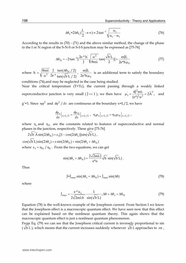
max s N maxJ=J sin( ) J sin( ) (78)

where

smax s N

' '

e * 1J . ,

2 2m b sin( b L)

(79)

Equation (78) is the well-known example of the Josephson current. From Section I we know

that the Josephson effect is a macroscopic quantum effect. We have seen now that this effect

can be explained based on the nonlinear quantum theory. This again shows that the

macroscopic quantum effect is just a nonlinear quantum phenomenon.

From Eq. (79) we can see that the Josephson critical current is inversely proportional to sin

( 'b L ), which means that the current increases suddenly whenever 'b L approaches to n ,

www.intechopen.com


199

suggesting some resonant phenomena occurs in the system． This has not been observed

before. Moreover maxJ is proportional to 'se * / 2 2m b S N(e* /4m ) , which is

related to (T-Tc)2．

Finally, it is worthwhile to mention that no explicit assumption was made in the above on

whether the junction is a potential well ( <0) or a potential barrier ( >0). The results are

thus valid and the Josephson effect in Eq. (2.78), occurs for both potential wells and for

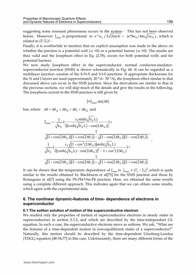
potential barriers. We now study Josephson effect in the superconductor -normal conductor-insulator-superconductor junction (SNIS) is shown schematically in Fig. 6b. It can be regarded as a multilayer junction consists of the S-N-S and S-I-S junctions. If appropriate thicknesses for the N and I layers are used (approximately 20 °A– 30 °A), the Josephson effect similar to that discussed above can occur in the SNIS junction. Since the derivations are similar to that in the previous sections, we will skip much of the details and give the results in the following. The Josephson current in the SNIS junction is still given by

maxJ=J sin( )

but, where s1 N s2I and

'1

max' '

2 '1

' ' 2 2

sinh( b L)1J { }

b 2[cosh( b L) cos(2 )]

1

[1 cos(2 )][1 cos(2 )] [1 cos(2 )][1 cos(2 )]

[1 cos (2 )]sinh( b L)1{ }

b 2[cosh( b L) cos(2 )] 1 cos (2 )

1

[1 cos(2 )][1 cos(2 )]

N

N N N

N I N I

N N

N N N N

N I

[1 cos(2 )][1 cos(2 )]N I

,

It can be shown that the temperature dependence of maxJ is 2max 0( )cJ T T ,which is quite

similar to the results obtained by Blackburm et al[73] for the SNIS junction and those by

Romagnan et al[7] using the Pb-PbO-Sn-Pb junction. Here, we obtained the same results

using a complete different approach. This indicates again that we can obtain some results,

which agree with the experimental data.

6. The nonlinear dynamic-features of time- dependence of electrons in superconductor

6.1 The soliton solution of motion of the superconductive electron

We studied only the properties of motion of superconductive electrons in steady states in

superconductors in section 2.3.2, and which are described by the time-independent GL

equation. In such a case, the superconductive electrons move as solitons. We ask, “What are

the features of a time-dependent motion in non-equilibrium states of a superconductor?”

Naturally, this motion should be described by the time-dependent Ginzburg-Landau

(TDGL) equation [48-54,77] in this case. Unfortunately, there are many different forms of the

www.intechopen.com


200

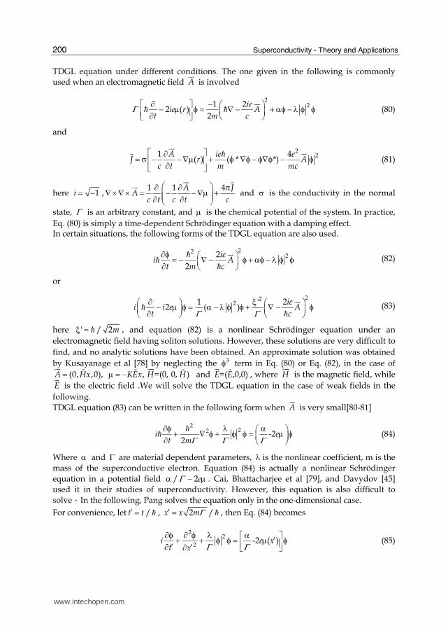
TDGL equation under different conditions. The one given in the following is commonly

used when an electromagnetic field A

is involved

2

21 22 ( )

2

ieie r A

t m c

(80)

and

2

21 4( ) ( * *)

A ie eJ r A

c t m mc

(81)

here 1i ,1 1 4A J

Ac t c t c

and is the conductivity in the normal

state, is an arbitrary constant, and is the chemical potential of the system. In practice,

Eq. (80) is simply a time-dependent Schrödinger equation with a damping effect. In certain situations, the following forms of the TDGL equation are also used.

22

22

2

iei A

t m c

(82)

or

22

21 ' 22 ( )

iei i e A

t c

(83)

here ' / 2m , and equation (82) is a nonlinear Schrödinger equation under an

electromagnetic field having soliton solutions. However, these solutions are very difficult to

find, and no analytic solutions have been obtained. An approximate solution was obtained

by Kusayanage et al [78] by neglecting the 3 term in Eq. (80) or Eq. (82), in the case of

(0, ,0),A Hx , =(0, 0, ) KEx H H and =( ,0,0)E E , where H

is the magnetic field, while

E

is the electric field .We will solve the TDGL equation in the case of weak fields in the

following.

TDGL equation (83) can be written in the following form when A

is very small[80-81]

2

22 -22

i et m

(84)

Where and are material dependent parameters, is the nonlinear coefficient, m is the

mass of the superconductive electron. Equation (84) is actually a nonlinear Schrödinger

equation in a potential field / 2e . Cai, Bhattacharjee et al [79], and Davydov [45]

used it in their studies of superconductivity. However, this equation is also difficult to

solve．In the following, Pang solves the equation only in the one-dimensional case.

For convenience, let /t t , 2 /x x m , then Eq. (84) becomes

2

2

2-2 ( )i e x

t x

(85)

www.intechopen.com


201

If we let 2 0e , then Eq. (85) is the usual nonlinear Schrödinger equation whose

solution is of the form [80-81]

0 ( , )00( , ) ,i x t

s x t e (86)

2 2

0

( 2 ) ( 2 )( , ) sec ( )

2 4e c e e c e

ex t h x t

(87)

here 0

1( , ) ( )

2e cx t x t . In the case of -2 0e

, let KEx , where K is a constant,

and assume that the solution is of the form [80-81]

( , )'( , ) i x tx t e (88)

Substituting Eq. (88) into Eq. (86), we get:

2 2

32

'' ' ( ') 2 '

( )KeEx

t t x

(89)

2

2

' '2 ' 0

( )t x x x

(90)

Now let '( , ) ( ),x t ( ),x u t ( )u t 22 ( )EKe t t d , where ( ')u t describes the

accelerated motion of '( , )x t . The boundary condition at requires ( ) to approach

zero rapidly. When 2 0u , equation (90) can be written as: 2 ( )

( / 2)

g t

u

, or

2

( )

2

g t u

x

(91)

where / 'u du dt . Integration of (91) yields:

20

''( , ) ( ) ( )

2

x dx ux t g t x h t

(92)

and where ( ')h t is an undetermined constant of integration. From Eq. (92) we can get:

02 2 20

''( ) ( )

2

x

x

gu gudx ug t x h t

t

(93)

Substituting Eqs. (92) and (93) into Eq. (89), we have:

22 2

302 2 2 30

''2 ( )

2 4( )

x

x

gu gu u dxKEex x h t g

x

(94)

www.intechopen.com


202

Since2

2( )x

=

2

2

d

d

, which is a function of only, the right-hand side of Eq. (94) is also a

function of only, so it is necessary that 0( ) constantg t g , and

'

2' ' '

2 x 0

guu u(2KEex + )+ x h(t )+ ( )

2 4 fV

. Next, we assume that 0( ) ( )V V , where

is real and arbitrary, then

2

0 022 ( ) ( )

2 4x

guu uKEex V x h t

(95)

Clearly in the case discussed, 0( )V 0, and the function in the brackets in Eq. (95) is a

function of t. Substituting Eq. (95) into Eq. (94), we can get [80-81]:

23 32

02/g

(96)

This shows that is the solution of Eq. (96) when and g are constant. For large , we

may assume that 1/

, when is a small constant. To ensure that and 2 2d d

approach zero when → , only the solution corresponding to g0=0 in Eq. (96) is kept, and

it can be shown that this soliton solution is stable in such a case. Therefore, we choose g0=0

and obtain the following from Eq. (91):

/ /2x u (97)

Thus, we obtain from Eq. (95) that

2' ' 'u u

2KEex + x h(t )-2 4

,

2 2 3 21 4( ) ( ) ( ) ( )

4 3

h t t KEe t e KE t (98)

Substituting Eq. (98) into Eqs. (92) - (93), we obtain:

2 2 3 21 1 42 ( ) ( ) ( )

2 4 3KEet x t KEe t e KE t

(99)

Finally, substituting the Eq. (99) into Eq. (96), we can get

23

20

(100)

When 0 , the solution of. Eq. (100) is of the form

2sech

(101)

Thus [80-81]

www.intechopen.com


203

2

2

2 3 22

2 3

2 2 2sec

2 2 1 4( )exp

2 4 3

m eKEt t dh x

eKEt m t eKE t KeEti x

(102)

This is also a soliton solution, but its shape，amplitude and velocity have been changed relatively as compared to that of Eq. (87). It can be shown that Eq. (102) does indeed satisfy Eq. (85). Thus, equation (85) has a soliton solution. It can also be shown that this solition solution is stable.

6.2 The properties of soliton motion of the superconductive electrons For the solution of Eq. (102), we may define a generalized time-dependent wave number,

22

k KEetx

and a frequency

2 2 2

2

12 ( ) ( )

4

2 2

KEex e KEe tt

KEe t KEex k

(103)

The usual Hamilton equations for the superconductive electron (soliton) in the macroscopic

quantum systems are still valid here and can be written as [80-81] 2k

dkKEe

dt x

,

then the group velocity of the superconductive electron is

2 2 42

g x

dxKEet KEet

dt k

(104)

This means that the frequency ω still represents the meaning of Hamiltonian in the case of

nonlinear quantum systems. Hence, 0x k

d d dk dx

dt dk dt x dt

, as seen in the usual

stationary linear medium.

These relations in Eqs. (103)-(104) show that the superconductive electrons move as if they

were classical particles moving with a constant acceleration in the invariant electric-field,

and that the acceleration is given by 4KEe . If >0, the soliton initially travels toward the

overdense region, it then suffers a deceleration and its velocity changes sign. The soliton is

then reflected and accelerated toward the underdense region.The penetration distance into

the overdense region depends on the initial velocity . From the above studies we see that the time-dependent motion of superconductive electrons still behaves like a soliton in non-equilibrium state of superconductor. Therefore, we can conclude that the electrons in the superconductors are essentially a soliton in both time-independent steady state and time-dependent dynamic state systems. This means that the soliton motion of the superconductive electrons causes the superconductivity of material. Then the superconductors have a complete conductivity and nonresistance property

www.intechopen.com


204

because the solitons can move over a macroscopic distances retaining its amplitude, velocity, energy and other quasiparticle features. In such a case the motions of the electrons in the superconductors are described by a nonlinear Schrödinger equations (52), or (53) or (80) or (82) or (84). According to the soliton theory, the electrons in the superconductors are localized and have a wave-corpuscle duality due to the nonlinear interaction, which is completely different from those in the quantum mechanics. Therefore, the electrons in superconductors should be described in nonlinear quantum mechanics[16-17].

7. The transmission features of magnetic-flux lines in the Josephson junctions

7.1 The transmission equation of magnetic-flux lines

We have learned that in a homogeneous bulk superconductor, the phase ( , )r t of the

electron wave function ,, ,

i r tr t f r t e

is constant, independent of position and time.

However, in an inhomogeneous superconductor such as a superconductive junction

discussed above, becomes dependent of r

and t. In the previous section, we discussed

the Josephson effects in the S-N-S or S-I-S, and SNIS junctions starting from the

Hamiltonican and the Ginzburg-Landau equations satisfied by ,r t , and showed that the

Josephson current, whether dc or ac, is a function of the phase change, 1 2 . The

dependence of the Josephson current on is clearly seen in Eq. (78) . This clearly indicates

that the Josephson current is caused by the phase change of the superconductive electrons.

Josephson himself derived the equations satisfied by the phase difference , known as the

Josephson relations, through his studies on both the dc and ac Josephson effects. The

Josephson relations for the Josephson effects in superconductor junctions can be

summarized as the following,

sin ,s mJ J 2eVt

, 2 ' /yed H cx

, 2 ' /xed H cy

(105)

where d’ is the thickness of the junction. Because the voltage V and magnetic field H

are

not determined, equation (105) is not a set of complete equations. Generally, these equations

are solved simultaneously with the Maxwell equation (4 / )H c J . Assuming that the

magnetic field is applied in the xy plane, i.e. ( , ,0)x yH H H, the above Maxwell equation

becomes

4

( , , ) ( , , ) ( , , )y xH x y t H x y t J x y tx y c

(106)

In this case, the total current in the junction is given by 0( , , ) ( , , ) ( , , )s n dJ J x y t J x y t J x y t J

In the above equation, ( , , )sJ x y t is the superconductive current density, ( , , )nJ x y t is the

normal current density in the junction (Jn =V/R(V ) if the resistance in the junction is R(V )

and a voltage V is applied at two ends of the junction), ( , , )dJ x y t is called a displacement

current and it is given by ( ) /dJ CdV t dt , where C is the capacity of the junction, and 0J is a

constant current density. Solving the equations in Eqs,(102) and (106) simultaneously, we

can get

www.intechopen.com


205

2

22

0 02 20

1 1( ) sin

J

Itv t

(107)

where 20 0/ 4 ', 1 / ,v c Cd RC 2 2

0 0/ 4 ' * , 4 * / , * 2J c d e I e J c e e . Equation (107) is the equation satisfied by the phase difference. It is a Sine-Gordon equation

(SGE) with a dissipative term. From Eq.(105), we see that the phase difference depends on

the external magnetic field H

, thus the magnetic flux in the junction

'*

cHds A dl dl

c can be specified in terms of , where A

is vector potential of

electromagnetic field, dl

is line element of vortex lines. Equation (107) represents

transmission of superconductive vortex lines. It is a nonlinear equation. Therefore, we know

clearly that the Josephson effect and the related transmission of the vortex line, or magnetic

flux, along the junctions are also nonlinear problems. The Sine-Gordon equation given

above has been extensively studied by many scientists including Kivshar and Malomed[39-

40]. We will solve it here using different approaches.

7.2 The transmission features of magnetic-flux lines

Assuming that the resistance R in the junction is very high, so that 0nJ , or equivivalently

0 0 , setting also I0 = 0, equation (107) reduces to

2

22

2 20

1 1sin

Jv t

(108)

Define 0/ , /J JX x T v t , then in one-dimension, the above equation becomes

2 2

2 2

sinX T

which is the 1D Sine-Gordon equation. If we further assume that ( , ) ( ')X T with

'0 0 0' ' ', ' / / 2 , ' / 2 /X X vT X X hc LI e T T I e hc

it becomes 2 2'(1 ) ( ') 2( ' cos )v A ,where A’ is a constant of integration. Thus

0

( ') 1/2[( ' cos )] 2 'A d

where 21 / 1 , 1v . Choosing A’=1, we have

1/2( ')[sin( / 2)] 2 'd

A kink soliton solution can be obtained as follows ' ln[tan( / 2)], 'or 1( ') 4 tan [exp( ')] . Thus yields

1 '0( ', ') 4 tan {exp[ ( ' ')]}X T X X vT (109)

www.intechopen.com


206

From the Josephson relations, the electric potential difference across the junction can be

written as

'0 002

22 sec [ ( ' ')]

2 ' 2 ' 2oI ed d

V v h X X vTe dT c dT cc

where 7 20 2 10 /c Gauss cm 'is a quantum fluxon, c is the speed of light. A similar

expression can be derived for the magnetic field

'0 002

22 sec [ ( ' ')]

2 ' 2 ' 2o

zI ed d

H h X X vTe dX c dX cc

We can then determine the magnetic flux through a junction with a length of L and a cross

section of 1 cm2. The result is

'0 0' ( , ) ( ', ') 'x xH x t dx B H X T dX

Therefore, the kink ( 1 ) carries a single quantum of magnetic flux in the extended

Josephson junction. Such an excitation is often called a fluxon, and the Sine-Gordon

equation or Eq.(107) is often referred to as transmission equation of quantum flux or fluxon.

The excitation corresponding to = −1 is called an antifluxon. Fluxon is an extremely stable

formation. However, it can be easily controlled with the help of external effects. It may be

used as a basic unit of information.

This result shows clearly that magnetic flux in superconductors is quantized and this is a

macroscopic quantum effect as mentioned in Section 1. The transmission of the quantum

magnetic flux through the superconductive junctions is described by the above nonlinear

dynamic equation (107) or (108).The energy of the soliton can be determined and it is given by 28 / ,E m where 2 2/ 1 / Jm .

However, the boundary conditions must be considered for real superconductors. Various

boundary conditions have been considered and studied. For example, we can assume the

following boundary conditions for a 1D superconductor, (0, ) ( , ) 0x xt L t . Lamb[47]

obtained the following soliton solution for the SG equation (108)

1( , ) 4 tan [ ( ) ( )]x t h x g t

(110)

where h and g are the general Jacobian elliptical functions and satisfy the following

equations

2 4 2[ ( )] ' (1 ') ',h x a h b h c 2 4 2[ ( )] ' ' 'g x c h b h a

with a’, b’, and c’ being arbitrary constants. Coustabile et al. also gave the plasma oscillation,

breathing oscillation and vortex line oscillation solutions for the SG equation under certain

boundary conditions. All of these can be regarded as the soliton solution under the given

conditions.

Solutions of Eq.(108) in two and three-dimensional cases can also be found[80-81]. In two-

dimensional case, the solution is given by

www.intechopen.com


207

1 ( , , )( , , ) 4 tan [ ]

( , , )

g X Y TX Y T

f X Y T (111)

where 0/ , / , /J J JX x Y y T v t , 1 2 2 3 1 31 (1,2) (2,3) (3,1)y y y y y yf a e a e a e ,

1 2 1 2 3(1,2) (2,3) (3,1)y y y y yg e e a a a e

and

0 2 2 21 , 1,( 1,2,3)i i i i i i iy p X q Y y p q i

2 2 2

2 2 2

( ) ( ) ( )( , ) ,(1 3)

( ) ( ) ( )

i j i j i j

i j i j i j

p p q qa i j i j

p p q q

In addition, Pi, qi and i satisfy 1 1 1

2 2 2

3 3

det 0

3

p q

p q

p q

. In the three-dimensional case, the

solution is given by

1 ( , , , )( , , , ) 4 tan [ ],

( , , , )

g X Y Z TX Y Z T

f X Y Z T , (112)

where X, Y , and T are similarly defined as in the 2D case given above, and / JZ z . The

functions f and g are defined as

1 2 2 3 1 32 3 3 1y y y y y yf dX e dY e dZ e , 1 2 3 1 2 3

2 3 3y y y y y yg e e e dX dY dZ e ,

2 2 2 21 2 3 1 2 3, 1,( , , )i i i i i i i i i iy a X a Y a b T C a a a b i X Y Z

with

3 2 2

13 2 2

[( ) ( ) ]( , ) ,(1 3),

[( ) ( ) ]

ik jk i jk

ik jk i jk

a a b bd i j j

a a b b

here 3y is a linear combination of 1y and 2y , i.e., 3 1 2y y y .

We now discuss the SG equation with a dissipative term 0 / t . First we make the

following substitutions to simplify the equation

2 20 0 0 0/ , / / , / , ' .J J J J JX x T v t t a v B I

In terms of these new parameters, the 1D SG equation (107) can be rewritten as

2

2 2

2sin 'a B

TX T

(113)

The analytical solution of Eq.(113) is not easily found. Now let

www.intechopen.com


208

20 0 0

2 2 200 0

1 1, , ' , '

1

v X v T avq

ava v v

(114)

Equation (113) then becomes

2

2' sin ' 0q B

(115)

This equation is the same as that of a pendulum being driven by a constant external moment

and a frictional force which is proportional to the angular displacement. The solution of the

latter is well known, generally there exists an stable soliton solution[80-81]. Let '/Y d d ,

equation (115) can be written as

' sin ' ' 0Y

q Y B (116)

For 0 ' 1B , we can let 0 0' sin (0 / 2)B and 0 1' , then, equation (116)

becomes

0 1 0' sin sin( )Y

Y q Y (117)

Expand Y as a power series of 1 , i.e., 1 ,nnn

Y c and inserting it into Eq.(117), and

comparing coefficients of terms of the same power of 1 on both sides, we get

2

01 0 2

1

' ' sin1cos ,

2 4 ' 3 2

q qc c

q c

, 2 0 03 2 4 2 3

1 1

cos sin1 1( 2 ), ( 5 )

' 4 6 ' 5 24c c c c c

q c q c

(118)

and so on. Substituting these 'nc s into 21'/ ,nn

Y d d c the solution of 1 may be

found by integrating 21 1/ nn

d c . In general, this equation has soliton solution or

elliptical wave solution. For example, when 2 31 1 2 1 3 1'/d d c c c it can be found that

1 12( ,sin ( ))

A B AF

A C A BA C

where 1( , )F k is the first Legendre elliptical integral, and A, B and C are constants. The

inverse function 1 of 1( , )F k is the Jacobian amplitude ' 1 amF . Thus,

1 1sin ( )A A C

amA B A B

or 1 ) ( )A A C

snA B A B

where snF is the Jacobian sine function. Introducing the symbol cscF = 1/snF, the solution can be written as

21 ( )[csc( )]

A CA A B

A B

(119)

www.intechopen.com


209

This is a elliptic function. It can be shown that the corresponding solution at is a

solitary wave.

It can be seen from the above discussion that the quantum magnetic flux lines (vortex lines)

move along a superconductive junction in the form of solitons. The transmission velocity 0v

can be obtained from 20 01h v v and nc in Eq. (118) and it is given by

20 01 / 1 [ / ( )]v h .

That is, the transmission velocity of the vortex lines depends on the current 0I injected and

the characteristic decaying constant of the Josephson junction. When is finite, the

greater the injection current I0 is, the faster the transmission velocity will be; and when I0 is

finite, the greater the is, the smaller the 0v will be, which are realistic.

8. Conclusions

We here first reviewed the properties of superconductivity and macroscopic quantum effects, which are different from the microscopic quantum effects, obtained from some experiments. The macroscopic quantum effects occurred on the macroscopic scale are caused by the collective motions of microscopic particles , such as electrons in superconductors, after the symmetry of the system is broken due to nonlinear interactions. Such interactions result in Bose condensation and self-coherence of particles in these systems. Meanwhile, we also studied the properties of motion of superconductive electrons, and arrived at the soliton solutions of time-independent and time-dependent Ginzburg-Landau equation in superconductor, which are, in essence, a kind of nonlinear Schrödinger equation. These solitons, with wave-corpuscle duality, are due to the nonlinear interactions arising from the electron-phonon interaction in superconductors, in which the nonlinear interaction suppresses the dispersive effect of the kinetic energy in these dynamic equations, thus a soliton states of the superconductive electrons, which can move over a macroscopic distances retaining the energy, momuntum and other quasiparticle properties in the systems, are formed. Meanwhile, we used these dynamic equations and their soliton solutions to obtain, and explain, these macroscopic quantum effects and superconductivity of the systems. Effects such as quantization of magnetic flux in superconductors and the Josephson effect of superconductivity junctions,thus we concluded that the superconductivity and macroscopic quantum effects are a kind of nonlinear quantum effects and arise from the soliton motions of superconductive electrons. This shows clearly that studying the essences of macroscopic quantum effects and properties of motion of microscopic particles in the superconductors has important significance of physics.

9. References

[1] Parks, R. D., Superconductivity, Marcel. Dekker, 1969. [2] Rogovin, D. and M. Scully, Superconductiviand macroscopic quantum phenomena,

Phys. Rep. 25(1976) 178. [3] Rogovin, D., Electrodynamics of Josephson junctions，Phys. Rev. B11 (1975) 1906-108 [4] Abrikosov, A. A. and L. P. Gorkov, I.V. Dzyaloshinkii, Quantum field theoretical

mothods in statistic phyics, Pregamon Press, Oxfordea, 1965 [5] Rogovin, D., Josephson tunneling: An example of steady-state superradiance,Phys. Rev.

B12 (1975) 130-133.

www.intechopen.com


210

[6] Ginzburg V L, Superconductivity, Superdiamagnetism, Superfluidity , Moscow: MIR Publ., 1987

[7] Ginzburg V L, Superconductivity, Moscow-Leningrad: Izd. Moscoew, AN SSSR, 1946 [8] Ginzburg, V. L.. Superconductivity and superfluidity Phys.-Usp. 40 (1997 ) 407 [9] Leggett, A. J., Macroscopic Effect of P- and T-Nonconserving Interactions in

Ferroelectrics: A Possible Experiment? Phys. Rev. Lett. 41 (1978) 586 [10] Leggett, A. J., in Percolation, Localization and Superconductivity, eds. by A. M.

Goldlinan,S. A. Bvilf, Plenum Press, New York, 1984. pp. 1- 41. [11] Leggett, A. J., Low temperature physics, Springer, Berlin, 1991, pp. 1-93; [12] Pang Xiao-feng, Investigations of properties of motion of superconductive electrons in

superconductors by nonlinear quantum mechanics, J. Electronic Science and Technology of China, 6(2)(2008)205-211

[13] Pang, Xiao-feng, macroscopic quantum effects, Chinese J. Nature, 5 (1982) 254, [14] Pang Xiao-feng, Investigations of properties and essences of macroscopic quantum

effects in superconductors by nonlinear quantum mechanics, Nature Sciences, 2(1)(2007) 42

[15] Pang, Xiao-feng, Investigation of solutions of a time-dependent Ginzburg-Landau equation in superconductor by nonlinear quantumtheory, IEEE Compendex, 2009, 274-277, DOI: 10.1109/ ASEMD.2009.5306641(EI)

[16] Pang, Xiao-feng, Theory of Nonlinear Quantum Mechanics, Chongqing Press, Chongqing, 1994.p35-97

[17] Pang Xiao-feng Nonlinear Quantum Mechanics, Beijing, Chinese Electronic Industry Press, Beijing, 2009,p20-63

[18] Bardeen, L. N., L. N. Cooper and J. R. Schrieffer, Superconductivity theory, Phys. Rev. 108 (1957) 1175;

[19] Cooper, L. N., The bound electronic pairs in degenerated Fermi gas Phys. Rev. 104 (1956) 1189.

[20] Schrieffer, J. R., Superconductivity, Benjamin, New York, 1969. [21] Schrieffer, J. R., Theory of Superconductivity, Benjamin, New York, 1964. [22] Frohlich.H., Theory of superconductive states, Phys. Rev.79(1950)845; [23] Frohlich.H., On superconductivity theory : one-dimensional case, Proc. Roy.Soc.A,

223(1954)296 [24] Josephson, B.D, Possible New Effects in Superconducting Tunnelling , Phys. Lett. 1

(1962) 251 [25] Josephson, B.D, Supercurrents through barriers, Adv. Phys. 14 (1965) 419. [26] Josephson, B.D., Thesis, unpublised, Cambridge University (1964) [27] Pang, Xiao-feng, The relation between the physical parameters and effective spectrum

of phonon, Southwest Inst. For Nationalities, . 17 (1991) 1. [28] Pang, Xiao-feng, On the solutions of the time-dependent Ginzburg-Landau equations

for a superconductor in a weak field, J. Low Temp. Physics, 58(1985)333 [29] Pang, Xiao-feng, The isotope effects of superconductor, Chinese. J. Low Temp.

Supercond.,No. 3 (1982) 62 [30] Pang, Xiao-feng, The properties of soliton motion for superconductivity electrons. Proc.

ICNP, Shanghai, 1989, p139. [31] Rayfield, G. W. and F. Reif, Evidence for the creation and motion of quantized vortex

rings in superfluid helium, Phys. Rev. Lett. 11 (1963) 305. [32] Perring, J. K., and T.H.R.Skyrme, A model unified field equation,Nucl. Phys. 31 (1962)

550.

www.intechopen.com


211

[33] Barenghi, C. F., R. J. Donnerlly and W. F.Vinen, Quantized Vortex Dynamics and Superfluid Turbulence, Springer, Berlin, 2001.

[34] Bogoliubov, N. N., Quantum statistics, Nauka, Moscow, 1949 [35] Bogoliubov, N. N., V. V. Toimachev and D. V. Shirkov, A New Method in the Theory of

Superconductivity, AN SSSR, Moscow, 1958. [36] London, F., superfluids Vol.1, Weley, New York 1950. [37] de Gennes, P. G., Superconductivity of Metals and Alloys, W. A. Benjamin, New York,

1966. [38] Suint-James, D., et al., Type-II Superconductivity, Pergamon, Oxford, 1966. [39] Kivshar, Yu. S. and B. A. Malomed, Dynamics of solitons in nearly integrable

systems，Rev. Mod. Phys. 61 (1989) 763. [40] Kivshar, Yu. S., T. J. Alexander and S. K. Turitsy, Nonlinear modes of a macroscopic

quantum oscillator， Phys. Lett. A 278(2001) 225. [41] Bullough, R. K., N. M. Bogolyubov, V. S. Kapitonov, C. Malyshev, J. Timonen, A. V.

J.Rybin, A.V., Vazugin, G.G. and Lindberg, M, Quantum integrable and nonintegrable nonlinear Schrodinger models for realizable Bose-Einstein condensation in d+1 dimensions (d=1,2,3)， Theor. Math.Phys. 134(2003)47

[42] Bullough, R. K. and P. T. Caudeey, Solitons, Plenum Press, New York, 1980. [43] Huepe, C. and M. E. Brachet, Scaling laws for vortical nucleation solutions in a model of

superflow，Physica D 140 (2000) 126. [44] Sonin, E. B., Nucleation and creep of vortices in superfluids and clean

superconductors,Physica，B210′1995″234-250 [45] Davydov.A.S. and V.N.Ermakov, Stability of a Superconducting Condensate of

Bisolitons, Phys. Stat.Sol.B148(1988)305 [46] Landau, L. D. and E. M. Lifshitz, Quantum mechanics, Pergamon Press, Oxford, 1987 [47] Lamb, G. L., Analytical descriptions of ultrashort optical pulse propagation in a

resonant medium，Rev. Mod. Phys. 43 (1971) 99. [48] Ginzberg, V. L. and L. D. Landau, On the theory of superconductivity，Zh. Eksp.

Theor. Fiz. 20 (1950) 1064; [49] Ginzburg V.L., On superconductivity and superfluidity, Physics –Usp. 47 (2004) 1155 -

1170 [50] Ginzberg, V. L. and D. A. Kirahnits, Problems in High-Temperature Superconductivity,

Nauka, Moscow, 1977. [51] Gorkov, L. P., On the energy spectrum of superconductors, Sov. Phys. JETP 7(1958) 505. [52] Gorkov, L. P., Microscopic derivation of the Ginzburg-Landau equation in the theory of

superconductivity, Sov. Phys. JETP 9 (1959) 1364. [53] Abrikosov, A. A., On the magnetic properties of superconductors of the second

group，Zh. Eksp. Theor. Fiz. 32 (1957) 1442. [54] Abrikosov, A. A. and L. P. Gorkov, Zh. Eksp. Theor. Phys. 39 (1960) 781; [55] Valatin. J.G. , Comments on the theory of superconductivity, Nuovo Cimento7(1958)843 [56] Liu, W. S. and X. P. Li, BCS states as squeezed fermion-pair states, European Phys. J. D2

(1998) 1. [57] Gross, E. F.,structure of a quantized vertex in boson systems, II Nuovo Cimento, 20

(1961) 454. [58] Pitaevskii, L. P.. Vortex lines in an imperfect Bose gas. Sov. Phys. JETP-USSR, 13 (1961)451 [59] Pitaevskii, L. P. and Stringari, S. Bose–Einstein Condensation. Oxford, Clarendon Press, 2003

www.intechopen.com


212

[60] Elyutin P. V. and A. N. Rogovenko, Stimulated transitions between the self-trapped states of the nonlinear Schrödinger equation, Phys. Rev. E63 (2001) 026610.

[61] Elyutin, P. V., Buryak A V, Gubernov V V, Sammut R A and Towers I N, Interaction of two one-dimensional Bose-Einstein solitons: Chaos and energy exchange, Phys. Rev. E64 (2001) 016607.

[62] Pang, Xiao-feng, The properties of motion of superconductive electrons in superconductor, J. XinJiang Univ. (nature) 5(1988)33

[63] Pang Xiao-feng, The G-L theory of superconductivity bin magnetic-superconductor, Investigations of metal materials, 12(1986) 31

[64] Perez-Garcia, V. M., M. Michinel and H. Herrero, Bose-Einstein solitons in highly asymmetric traps, Phys. Rev. A57 (1998) 3837.

[65] London, F. and H. London, The electromagnetic equations of the superconductor, Proc. Roy. Soc. (London) A 149 (1935) 71

[66] Pang, Xiao-feng, Interpretation of proximity effect in superconductive junctions by G-L theory, J. Kunming Tech. Sci. Univ., 14. (1989) 78

[67] Pang, Xiao-feng, Properties of transmission of vortex lines along the superconductive junctions. J. Kunming Tech. Sci. Univ., 14 (1989) 83.

[68] Caradoc-Davies, B. M., R. J. Ballagh and K. Bumett, Coherent Dynamics of Vortex Formation in Trapped Bose-Einstein Condensates, Phys. Rev. Lett. 83 (1999) 895.

[69] Matthews, M. R., B. P. Anderson*, P. C. Haljan, D. S. Hall†, C. E. Wieman, and E. A. Cornell, Vortices in a Bose-Einstein Condensate, Phys. Rev. Lett. 83 (1999) 2498.

[70] Madison, K. W., F. Chevy, W. Wohlleben, and J. Dalibard , Vortex formation in a stirred Bose-Einstein condensate, Phys. Rev. Lett. 84 (2000) 806.

[71] Tonomura A, Kasai H, Kamimura O, Matsuda T, Harada K, Yoshida T, Akashi T, Shimoyama J, Kishio K, Hanaguri T, Kitazawa K, Masui T, Tajima S, Koshizuka N, Gammel PL, Bishop D, Sasase M, Okayasu S, Observation of structures of chain vortices inside anisotropic high- Tc superconductors, Phys. Rev. Lett. 88( 2002) 237001

[72] Pang, Xiao-feng, Investigation of solutions of Josephson equation in three dimension superconductive junctions, J. Chinghai Normal Univ. Sin. No. 1 (1989) 37.

[73] Blackbunu, J. A., H.J.T. Smith and N.L. Rowell, Proximity effects and the generalized Ginzburg-Landau equation, Phys. Rev. B11 (1975) 1053.

[74] Jacobson, D. A., Ginzburg-Landau equations and the Josephson effect, Phys. Rev. B8 (1965) 1066;

[75] Pang, Xiao-feng, The Bose condensation properties of superconductive states, J. Science Exploration Sin. 1(4 )(1986) 70.

[76] Pang, Xiao-feng, The features of coherent state of superconductive states, J. Southwest Inst. For Nationalities Sin. 17 (1991) 18.

[77] Dewitt, B. S., Superconductors and Gravitational Drag, Phys. Rev. Lett. 16 (1966) 1092 [78] Kusayanage.E, T. Kawashima and K.Yamafuji,Flux flow in nonideal type-II

superconductor, J. Phys. Soc. Japan 33 (1972) 551. [79] Cai, S. Y. and A. Bhattacharjee, Ginzburg-Landau equation: A nonlinear model for the

radiation field of a free-electron laser, Phys. Rev. A43 (1991) 6934. [80] Pang, Xiao-feng, Soliton Physics, Press of Sichuan Sci. and Tech., Chengdu, 2003 [81] Guo Bai-lin and Pang Xiao-feng, solitons, Chinese Science Press, Beijing, 1987

www.intechopen.com

Superconductivity - Theory and ApplicationsEdited by Dr. Adir Luiz

ISBN 978-953-307-151-0Hard cover, 346 pagesPublisher InTechPublished online 18, July, 2011Published in print edition July, 2011

InTech EuropeUniversity Campus STeP Ri Slavka Krautzeka 83/A 51000 Rijeka, Croatia Phone: +385 (51) 770 447 Fax: +385 (51) 686 166www.intechopen.com

InTech ChinaUnit 405, Office Block, Hotel Equatorial Shanghai No.65, Yan An Road (West), Shanghai, 200040, China

Phone: +86-21-62489820 Fax: +86-21-62489821

Superconductivity was discovered in 1911 by Kamerlingh Onnes. Since the discovery of an oxidesuperconductor with critical temperature (Tc) approximately equal to 35 K (by Bednorz and Müller 1986), thereare a great number of laboratories all over the world involved in research of superconductors with high Tcvalues, the so-called â€œHigh-Tc superconductorsâ€ . This book contains 15 chapters reporting aboutinteresting research about theoretical and experimental aspects of superconductivity. You will find here a greatnumber of works about theories and properties of High-Tc superconductors (materials with Tc > 30 K). In afew chapters there are also discussions concerning low-Tc superconductors (Tc < 30 K). This book willcertainly encourage further experimental and theoretical research in new theories and new superconductingmaterials.

How to referenceIn order to correctly reference this scholarly work, feel free to copy and paste the following:

Pang Xiao-feng (2011). Properties of Macroscopic Quantum Effects and Dynamic Natures of Electrons inSuperconductors, Superconductivity - Theory and Applications, Dr. Adir Luiz (Ed.), ISBN: 978-953-307-151-0,InTech, Available from: http://www.intechopen.com/books/superconductivity-theory-and-applications/properties-of-macroscopic-quantum-effects-and-dynamic-natures-of-electrons-in-superconductors

© 2011 The Author(s). Licensee IntechOpen. This chapter is distributedunder the terms of the Creative Commons Attribution-NonCommercial-ShareAlike-3.0 License, which permits use, distribution and reproduction fornon-commercial purposes, provided the original is properly cited andderivative works building on this content are distributed under the samelicense.

https://creativecommons.org/licenses/by-nc-sa/3.0/

properties of macroscopic quantum effects and dynamic natures

Documents