PROPAGATION OFREFRACTION ERRORSIN TRIGONOMETRIC

HEIGHT TRAVERSING ANDGEODETIC LEVELLING

G. A. KHARAGHANI

November 1987

TECHNICAL REPORT NO. 132

PREFACE

In order to make our extensive series of technical reports more readily available, we have scanned the old master copies and produced electronic versions in Portable Document Format. The quality of the images varies depending on the quality of the originals. The images have not been converted to searchable text.

PROPAGATION OF REFRACTION ERRORS IN TRIGONOMETRIC HEIGHT TRAVERSING

AND GEODETIC LEVELLING

Gholam A. Kharaghani

Department of Surveying Engineering University of New Brunswick

P.O. Box 4400 Fredericton, N.B.

Canada E3B5A3

November 1987

PREFACE

This report is an unaltered printing of the author's M.Sc. thesis of the same

title, which was submitted to this Department in August 1987.

The thesis supervisor was Professor Adam Chrzanowski.

Any comments communicated to the author or to Dr. Chrzanowski will be

greatly appreciated.

ABSTRACT

The use of trigonometric height traversing as an

alternative to geodetic levelling has recently been given

considerable attention. A replacement for geodetic

levelling is sought to reduce the cost and to reduce the

uncertainty due to the refraction and other systematic

errors.

As in geodetic levelling, the atmospheric refraction

can be the main source of error in the trigonometric method.

This thesis investigates the propagation of refraction

errors in trigonometric height traversing. Three new models

for the temperature profile up to 4 m above the ground are

propos.ed and compared with the widely accepted Kukkamaki 's

temperature model. The results have shown that the new

models give better precision of fit and are easier to

utilize.

A computer simulation of the influence of refraction. in

trigonometric height traversing suggests that the

accumulation of the refraction effect becomes randomized to

a large extent over long traverses. It is concluded that the

accumulation of the refraction effect in short-range

trigonometric height traversing is within the limits of

Canadian specifications for the first order levelling.

- ii -

TABLE OF CONTENTS

ABSTRACT . . . . . . . . . . . . . . . . . . . • ii

LIST OF TABLES . . . .. . . . . . . . . . . . . . . . vi

LIST OF FIGURES •

ACKNOWLEDGEMENTS

. . . . . . . . . . . . . . • • • viii

. . . . . . . . . . . . . . . . . . . • xi

Chapter

1. INTRODUCTION . . . . . . . . . . . . . . . . . . 1

2. A REVIEW OF METHODS FOR THE DETERMINATION OF THE REFRACTION CORRECTION • • • • • • • • • • • 6

Determination of the Vertical Refraction Angle by the Meteorological Approach • • • • • • 7

Refractive index of air • • • • • . • • . • 7 Angle of refraction error • • • • • • • • • • . 9

Determination of the Vertical Refraction Angle Using Lasers of Different Wavelengths • . . 13

Angle of Refraction Derived from the Variance of the Angle-of-Arrival Fluctuations • 15

Determination of the Vertical Refraction Correction Using the Reflection Method • . . 16

Comments on the Discussed Methods ••••••.• 17

3. REFRACTION CORRECTION IN GEODETIC LEVELLING USING THE METEOROLOGICAL METHOD • • • • • • • • • • • 19

Refraction Correction Based on Direct Measurement of Temperature Gradient • • • • • • . • . . 20

Kukkamaki's equation for geodetic levelling refraction correction • • • • • • •

Refraction Correction Formulated in Terms of . 22

Sensible Heat Flux . • • • • • • • • • • • . 27 Review of the meteorological parameters • • • . 27 Thermal stability parameter •••••••••. 30 Profile of mean potential temperature gradients 31 The Angus-Leppan equation for refraction

correction • . • . • • • • • • • • . 35 • 36

. • 38 Investigation by Holdahl • • • • • • • •

Comments on the Meteorological Methods • • • •

- iii -

4. REFRACTION CORRECTION IN TRIGONOMETRIC HEIGHT TRAVERSING • • • • • • • • • • • • • • • • 39

Reciprocal Trigonometric Height Traversing •••• 41 Formulae of reciprocal trigonometric height

traversing • • • • • • • • • • • • • • . 42 Achievable accuracy using reciprocal

trigonometric height traversing • • . 44 Precision of refraction corrections in

reciprocal method • • • • • • • • • . 47 Proposed method for the calculation of

refraction correction • • • • • • • 49 Refraction in Leap-Frog Trigonometric Height

Traversing • • • • • • • • • • • • • • • • . 52 Leap-Frog Trigonometric Height Traversing

Formulae • • • • • • • • • • • • . . • • 53 Achievable Accuracy Using Leap-Frog

Trigonometric Height Traversing ••• 55 Precision of refraction correction in leap-

frog method • • • • • • • • • • • • . . • 56

5. TEST SURVEYS AT UNB •••••• . 59

Background of Trigonometric Height Traversing at UNB • • • • • • • • • • • • • • • • • • . • 59

Description of the Test Areas and Scope of the Tests . . . . . . . . . . . . . . . . . 61

South-Gym test lines • • • • • • • • • . • 61 Head-Hall test line • • • • • • • • • • . . 64

Description of the Field Equipment • • • • • . 66 Temperature gradient • • • • • • • • • • • • . 66 Trigonometric height traversing •••••••• 67

Investigation of Temperature Models as Function of Height . . . . . . . . . . . . . . . . . . . 67

Choice of models • o • • • • • • o o • • • • • 67 Temperature gradient measurement • o • • o • • 69 Determination of the coefficient of temperature

models . . . . . . . . . . . . . . . . . 7 4 Comparison and field verification of the

results • o • • • o o o • • • • •

Computed Versus Measured Refraction Effect . Tests on 20 June 1985 • • 0 • • • • • • •

Tests on 19 July 1985 o • • • • • o • • •

Tests on 23 and 24 July 1985 • . . • • • Tests on 29 July 1985 and estimation of

standard deviation of vertical angle measurements • • • • • • • • • • • o 0

Comments on South-Gym test surveys • • • o 0

Tests on 06 August 1985 • • • • • • • . . . •

6o SIMULATIONS OF REFRACTION ERROR IN TRIGONOMETRIC

. 83

. 93

. 93

. 95 100

112 115 116

HEIGHT TRAVERSING • • • • • • • • o • • • • • 120

- iv -

7.

Simulation Along a Geodetic Levelling Line on Vancouver Island • • • • • • • • • • • • • 120

Computation of the refraction error in geodetic levelling • • • • • • • • • • • • • • • 122

Refraction error in trigonometric height traversing • • • • • • • • • • • • • . 124

Results of simulations • • • • • • • • • • • 125 Simulation of the Refraction Error Using other

Values of Temperature Gradient Measurements 127 Simulation on the Test Lines at UNB • • • • 1.31

CONCLUSIONS AND RECOMMENDATIONS • . . . . Conclusions Recommendations

. . . . . . . . . . . . . . . . . . . . . . . . . . . . 145

145 149

REFERENCES . . . . . . . . . . . . . . . . . . . . . . 151

- v -

Table

5 .1.

5.2.

5.3.

5.4.

LIST OF TABLES

The Time Averaged Temperatures

The Time Averaged Temperatures

The Time Averaged Temperatures

Mean standard deviations . . .

on Gravel Line

on Grass Line . on Asphalt Line

. . . . . . . . 5.5. Curve fitting and coefficient of refraction

computations (Kukkamaki's model, i1 in Table

~

71

. . 72

. . 73

. . 75

5.4, over asphalt) ••••••••••••••• 77

5.6. Curve fitting and coefficient of refraction computations (model, i4 in Table 5.4, over asphalt) •••••••••••••.. 78

5.7. Curve fitting with test of the significance of coefficient (Kukkamaki's model, i1 in Table 5. 4) . . . . . . . . . . . . . . . . 80

5.8. Curve fitting with the significance of coefficient test (model i3 in Table 5.4). • .•.•.•• 81

5.9. Refraction effect [mm] computed using the seven models versus the measured value (BM1-BM2). . 86

5.10. Refraction effect [mm] computed using the seven models versus the measured value (BM2-BM3). • 87

5.11. Refraction effect [mm] computed using the seven models versus the measured value (BM3-BM1). . 88

5.12. Correlation Coefficients Matrices • 89

5.13. Preliminary test measurements using UNB trigonometric method at South-Gym area from BMl to BM2 • • • • • • • • • • • • • • • • • • • • 93

5.14. Discrepancies between the results obtained using trigonometric height traversing and geodetic levelling for BMl to BM2 •••••••••••. 96

- vi -

5.15. Discrepancies between the results obtained using trigonometric height traversing and geodetic levelling for BM2 to BM3 •••••••••••• 97

5.16. Discrepancies between the results obtained using trigonometric height traversing and geodetic levelling for BM3 to BMl ••...•••••.. 98

5.17. Computed refraction using measured temperature gradient . • • • • • • • • • • • • • • • • . . 99

5.18. t-test on the significance of the correlation coefficients • • • . • . . • • • . • • • • • 111

5.19. Computed refraction effect versus value for Head-Hall test line •

the measured 119

6.1. Average 6t, b and H along the levelling routes • 128

6.2. Average 6t, b and H in Fredericton, N.B •• 129

6.3. Average 6t, b and H along levelling routes in United States (after Holdahl [1982]) • • • • 130

- vii -

Figure

1.1.

2 .1.

2.2.

3 .1.

3.2.

LIST OF FIGURES

Methods of trigonometric height traversing • . . . 5

Vertical Refraction Angle . . . . . . . . . . . Principle of refraction by reflection . . . Refraction

up effect in a . . . . . . . geodetic levelling set-. •. . . . . .

• 10

. 17

• 23

Profile of mean potential temperature e • • 32

4.1. Ellipsoidal section for reciprocal trigonometric height traversing • • • • • • • • • • • • • • . 42

4.2. Standard deviation of refraction correction in reciprocal height traversing as a function of distance •••.••.••••••••••.•. 49

4.3. Ellipsoidal section for leap-Frog trigonometric height traversing • . • • • • • • • • • • • • . 54

4.4. Standard deviation of refraction correction in leap-frog height traversing as a function of distance. • • • • • . • • • • • • • • • • • 58

5 .1.

5.2.

5.3.

Plan and profiles of South-Gym test lines

Plan and profile of Head-Hall test line

Refraction Coefficient Contours . . . . . . . .

. 63

. 65

. 79

5.4. Test of the significance of coefficient for models in Table 5.4 .••.••.•••••••.•• 82

5.5. Refraction effect computed using the seven models versus the measured value for BM1-BM2 ••••• 90

5.6. Refraction effect computed using the seven models versus the measured value for BM2-BM3 ••... 91

5.7. Refraction effect computed using the seven models versus the measured value for BM3-BM1 .•.•. 92

- viii -

5.8. Back- and fore-sight magnitude of refraction difference • • • • • • • . • • • • • • • 100

5.9. Measured refraction effect versus the computed value. • • • • • • . . • • • • • • • • . 103

5.10. The measured refraction effect [mm]. • • • • 104

5.11. Fluctuations of point temperature gradient • 106

5.12. Fluctuations of observed vertical angles • • 107

5.13. Computed refraction effect versus the measured value. • • • • • • . • • . • • • • • 108

5.14. Linear correlation between the computed and measured refraction error. • • • • • • • 110

5.15. Measured refraction error versus the computed value. . . . . . . . . . . . . . . . . . . . 114

5.16. The discrepancies of height difference determined by trigonometric height traversing and geodetic levelling, between BM2 and BM4 at Head-Hall teat 1 ine. . • • • . • • • • • • • • • . . • . 117

6.1. Accumulation of refraction error in geodetic levelling using equations (3.19), (6.1) and (6.3) . . . . . . . . . . . . . . . . . . . . 133

6.2. Accumulation of refraction error in geodetic levelling and trigonometric height traversing along line i1 • • • • . . • • . • . • • • . . 134

6.3. Accumulation of refraction error in geodetic levelling and trigonometric height traversing along line t2 • • • . . • • • . • . • • • • . 135

6.4. Accumulation of refraction error in geodetic levelling and trigonometric height traversing along line i3 • • • . • . . • . • • • • • • • 136

6.5. Accumulation of refraction error in geodetic levelling and trigonometric height traversing along line i4 • • • . • • • • • • • • • . 137

6.6. Variations of turbulent heat flux along the levelling line +2 • . • • • • • • • • • • 138

6.7. Accumulation of refraction error in geodetic levelling and trigonometric height traversing (line i2) • . • • • . • • • • . • • • • . • . 139

- ix -

6.8. Accumulation of refraction error in geodetic levelling and trigonometric height traversing (line i4) • • • • • . • • • • • • • • • • 140

6.9. Refraction correction for line BM1-BM2 • 141

6.10. Refraction correction for line BM2-BM3 • •

6.11. Refraction correction for line BM3-BM1 •

. . . 142

143

6.12. Refraction correction for the Head-Hall test line 144

- X -

ACKNOWLEDGEMENTS

I wish to express my deepest gratitude and sincere

thanks to my supervisor, Dr. Adam Chrzanowski. His interest

in the topic and constructive suggestions were invaluable.

His guidance, immeasurable support and continuous

encouragement throughout the course of this work were highly

appreciated.

In addition, I would like to thank Dr. Yong-Qi Chen

from Wuhan Technical University of Surveying and Mapping for

his many hours spent in discussion and reading the original

manuscript and for his constructive criticism while he was

on leave at the Department of Surveying Engineering,

University of New Brunswick. I also wish to thank Dr.

Wolfgang Faig for his critical review of this thesis and for

his guidance and sound advice.

I would like to express my sincere thanks to Mr. James

Secord who spent many long hours to discuss, to read and to

render my difficult script into a readable form.

I am indebted to Dr. A. Jarzymowski a visiting scholar

from Poland for his help in making the meteorological

measurements possible and his assisstance during long days

of field work.

- xi -

xii

My thanks are extended also to many of my colleaques

for their generous assistance with the field work. Among

them, Messrs J. Kornacki, J. Mantha, C. Faig, K. Donkin, P.

Romero, z. Shi and M. Katekyeza are particularly thanked.

Thanks are also due to the personnel at the Geodetic

Survey of Canada for providing the data used in this study.

The work described in this

supported by the Geodetic Survey

thesis has been financially

of Canada,

Science and Engineering Research

University of New Brunswick.

Council

the National

and by the

Chapter 1

INTRODUCTION

The refractive properties of the atmosphere have placed

a limit on the accuracy of conventional geodetic levelling.

Geodetic levelling is a slow survey procedure which is

confined by its horizontal line of sight. Along inclined

terrain, refraction influences the measurements

systematically because the horizontal line of sight passes

obliquely through different isothermal layers of air. Under

certain extreme conditions such as the long easy gradient

along railways, an accumulation in the order 20 mm per 100 m

of height difference can be expected [Bamford, 1971]. A

suggested remedy is to shorten the sight length, because the

influence of refraction is proportional to the square of the

sight distance [e.g. Angus-Leppan, 1985]. For precise

levelling, Bamford [1971] recommends keeping the length of

sight under 30 m, even though the slope may allow longer

lengths. This restriction makes the survey progress even

slower and more expensive.

Because of these reasons, developement has been

intiated in the last few years to increase production and

reduce the systematic error effects by using the

trigonometric height traversing method as an alternative to

- 1 -

2

geodetic levelling. In the trigonometric methods, the

differences in elevations are determined

vertical angles and distances using the new

modern electronic theodolites and compact and

from measured

state-of-art

accurate EDM

(Electromagnetic Distance Measuring) instrumentation.

Two types of trigonometric height traversing can be

distinguished (see Figure 1.1):

1. Simultaneous reciprocal: the zenith angles are

measured in both directions simultaneously.

2. Leap-frog: the instrument is set up midway between

two target-reflector stations.

At the University of New Brunswick, the leap-frog method

with elevated multiple targets was developed and tested from

1981 to 1985. This variant of the leap-frog trigonometric

height traversing is called the "UNB-method".

In the trigonometric methods, vertical angle

observations are affected by the long-term temperature

gradient variations which cause vertical displacement of the

target image. The short-term temperature gradient

fluctuations cause the blurring of the image (image

dancing). As in geodetic levelling, the atmospheric

refraction can be the main source of error in the

trigonometric methods, though its systematic effect is

expected to be much smaller than in geodetic levelling.

Many authors have investigated both practical and

theoretical aspects of refraction error in geodetic

3

levelling [e.g. Kukkamaki 1938, Holdahl 1981, Angus-Leppan

1979b,l980]. These investigations have arrived at formulae

for the refraction correction, and practical experiments

have shown that the results from various formulae are

similar and are close to actual values [Angus-Leppan 1984,

Heer and Niemeier [1985), Banger 1982, Heroux et al. 1985].

These formulae are generally based on estimated (modelled)

or measured temperature gradients.

In the trigonometric methods, a similar refraction

correction can be derived if the lengths of sight are

compatiable with the length of sight used in geodetic

levelling, i.e. not exceeding 100 m. If the lines of sight

are longer, then the correction for refraction becomes a

more complicated task. On the other hand, as it will be

shown in this thesis, the influence of refraction in

trigonometric height traversing becomes randomized to a

large extent, if the lines of sight are short, i.e. less

than 100 m.

This thesis investigates the propagation of refraction

errors in the optical height difference determination

methods with more emphasis on the trigonometric height

traversing. The objectives can be summarized as follows:

1. To determine an optimal model for the

temperature profile

basis of several

up to 4 m

long term

typical ground surfaces (gravel,

above the ground on the

test surveys over three

grass and asphalt) and

4

profiles; to investigate the influence of refraction on

these surfaces and to compare the measured refraction

effect against the computed refraction correction.

2. To develop new models and to compare them against

the available models such as Kukkamaki's and Heer's

temperature functions.

3. To confirm in practice the designed precision of the

UNB-method under controlled field conditions, to add to

the understanding of the refraction effect and to

compare the UNB-method against the reciprocal method with

regard to the influence of refraction.

4. To simulate the refraction effect in the

trigonometric methods along a line of geodetic levelling,

to assess the dependence of

profile and to compare the

trigonometric methods versus

geodetic levelling.

the refraction errors on the

refraction effect in the

the refraction effect in

An overview of the solutions to the refraction problem

in optical height difference determination methods is given

in Chapters 2, 3 and 4. Chapter 2 reviews the method already

developed for the refraction correction computations based

on the evaluation of the temperature gradient, the so called

"meteorological method" and three other approaches namely:

1. the dispersion (the two wavelength system),

2. the variance of the angle-of-arrival, and

3. the refraction by reflection.

5

The development of these methods depends on further advances

in technology and they are promising a better performance

than the meteorological method [Brunner, 1979a;

Angus-Leppan, 1983]. Chapters 3 and 4 review in details

the meteorological approach in the optical height difference

determination methods. Chapter 4, also summarizes a new

approach in solving for the refraction effect in the

reciprocal method proposed by the author. Chapter 5 deals

with the 1985 test surveys, their analysis, and discussion

of results. The outcome of the simulations is given in

Chapter 6.

Figure 1.1: Methods of trigonometric heioht traversing (a) leap-frog (b) reciprocal

Chapter 2

A REVIEW OF METHODS FOR THE DETERMINATION OF THE REFRACTION CORRECTION

The most significant source of error in trigonometric

height traversing, as well as in geodetic levelling, is the

effect 6f atmospheric refraction. Several solutions are

suggested by different researchers. The most popular method

that has been applied in geodetic levelling is based on

temperature gradients which can be obtained either through

the direct measurements of air temperature at different

heights or by modelling the atmosphere using the theories of

atmospheric physics. This approach to the vertical

refraction angle computation is referred to, here, as the

meteorological method.

Besides the above method, the following three other

approaches are discussed in various literature. These

methods are [e.g. Brunner, 1979a; Angus-Leppan, 1983]:

1. Determination of the vertical angle of refraction

using using the dispersive property of the atmosphere.

2. Determination of the vertical angle of refraction

derived from the variance of the angle-of-arrival

fluctuations.

3. Determination of the vertical refraction correction

using the "reflection method" [Angus-Leppan, 1983].

- 6 -

7

This chapter summarizes the above methods. The

meteorological approach will be discussed with more detail

in Chapters 3 and 4.

2.1 Determination of the Vertical Refraction Angle hY the Meteorological Approach

2.1.1 Refractive index of air

Determination of errors due to atmospheric refraction

using the meteorological method requires knowledge of the

refraction properties of the atmosphere. The refractive

index n of a medium is defined as the ratio of the velocity

of light in a vacuum, co, to the velocity c of light in the

medium: n = C 0 /C. Variation in the refractive index of air

depends on the variation of temperature, pressure and

humidity. In 1960 a formula was adopted by the

International Association of Geodesy in terms of temperature

t [°C], pressure p [mb] and partial water vapour pressure

e [mb], which is [Bamford, 1971]:

1 p 4.2 e -8 (n- 1) = (no - 1).---------.-------- --------- 10

(1 + a t) 1013.25 (1 + a t)

(2.1)

where a = 1/273 = 0.00366 is the thermal expansion of air

and no is the refractive index of light in standard air at a

temperature 0 oc with a pressure of 1013.25 mb and with a

carbon dioxide content of 0.03% and is given by [e.g.

Hotine, 1969]

6 (no - 1) 10

8

-2 = 287.604 + 1.6288 A

-4 + 0.0136 ).. (2.2)

in which A is the wavelength [pm] of monochromatic light in

a vacuum. Substituting an average value of A = 0.56 pm for

white light and a = 0.00366 into equation (2.1) yields

-6 1 p (n - 1) = 293 x 10 ---------------

1 + 0.00366 t 1013.25

4.1 e -8 • 10 (2.3)

1 + 0.00366 t

The vertical gradient of the refractive index can be

expressed by differentiating equation (2.3) with respect to

z

dn 78.9 [ dp de = ------ ( - 0.14 ) -

dz T dz dz

p - 0.14 e dT l -6 ( ------------ ) ---- 10 (2.4)

T dz

where, T is the absolute temperature [.iq. In the second

term, 0.14 e, is negligible and 0.14 (de/dz) in normal

condition is less than 2% of ( dp/dz) and it can be

neglected [Bomford, 1971]. The vertical gradient of

pressure is approximated by [e.g. Bomford, 1971]

dp g p = - --- (2.5)

dz M T

9

where g is the gravitational acceleration and M is the

specific gas constant for dry air. In this equation, g/M has

the numerical value of 0.0342 K/m • This value is known as

the autoconvective lapse rate [Shaw and Smietana, 1982].

Lapse rate is the rate of decrease of temperature with

height. The simplified formula for vertical gradient of

the refractive index is then given by

dn .;...78.9 p dT -6 = ------- ( 0.0342 + ) 10 (2.6)

dz 2 dz T

In a homogeneous atmosphere, density is independent of

height. Equation (2.6) shows that under such conditions, a

lapse rate of -0.0342 K/m is necessary to compensate for the

decrease in atmospheric pressure with height.

2.1.2 Anqle of refraction error

Considering Figure 2.1 the vertical refraction angle oo

is the angle between the chord and the tangent to the

optical path AB. If dn/dz is known at all points along

AB, the vertical refraction angle can be calculated from the

eikonal (optical path length) equation [Brunner and

Angus-Leppan 1976]

sin z s 00 = ------- ~ dn/dz (S - X) dx (2.7)

s

where, s = the chord length AB,

z = the zenith angle, and

10

x = the distance along the chord.

z

A

- p -.._A \ \

---~

Figure 2.1: Vertical Refraction Ancle

Substituting equation {2.6) into (2.7)

sin Z = 1, gives

-6 10 s

00 = ------ ~ s

From Figure 2 .1,

c = - 00 • s R

( -78.9 p dT ------- { 0.0342 +

2 dz T

the refraction correction

and asaumin<J

) l (S - X) dx

{2.8)

is

(2.9)

11

The correction may be also calculated in terms of the

curvature of the light path and the coefficient of

refraction. The curvature is given by

1/p = - (dn/dz) . sin Z (2.10)

The coefficient of refraction is defined as the ratio of the

radius of the earth R to the radius of the curvature of

the light path

k = R I p (2.11)

Substituting equation (2.6) and (2.10) in (2.11) and

assuming R = 6371000 m gives

502.7 p dT k = -------- ( 0.0342 + ) (2.12)

2 dz T

Then equation (2.9) can be written as

1 s c = - (A) . s = - --- ~ k . (S-x) dx

R R (2.13)

In the simple case when the coefficient of refraction

is constant along the line of sight AB, the refraction angle

is given by

s (A) = ----- (2.14)

2 p

Substituting p from equation (2.11) into (2.14), gives

12

s k 00 = ----- (2.15)

2 R

Then, the refraction correction for a circular refraction

path (constant k along the line of sight) is

2 s

c = - ----- • k R 2 R

(2.16)

Which means that the refraction error is a function of the

square of the sight length.

Equation (2.8) shows that, in order to compute the

refraction angle, one needs to know the temperature

gradient, dT/dz, along the line of sight. Thus, dT/dz has

to be known as a function of height above the ground. The

temperature gradient can be obtained either by observing the

temperature of air at different heights above the ground and

then fitting these observed values to a temperature function

(see section 3.2), or by modelling in terms of sensible heat

flux and some other meteorological parameters •. Please refer

to Chapters 3 and 4 for a detailed discussion of the

refraction correction using meteorological method.

13

2.2 Determination of the Vertical Refraction Anale Usina Lasers of Different Wavelengths

The dispersive property of the atmosphere can be used

to determine the angle of refraction. In this approach the

fact that blue light is bent slightly more than red light

when propagating through a dispersive medium is used. A

dispersometer measures the angle between the arriving beams

of two different wavelengths by considering the time delay

or phase difference between two photomultiplier signals

related to the red and blue arriving refracted beams. Based

on this measurement, the angle between arriving beams, Aoo,

can be computed. This Aoo has to be multiplied by a known

factor V to obtain the angle of refraction oo [Williams and

Kahmen, 1984]

oo = V • Aoo (2.17)

in which V = N/AN, and N is the refractivity at standard

values of pressure and temperature. The value of N for dry

air at 288.15 K and 1013 mb is given by [Williams and

Kahmen, 1984] as

[ 24060.3 159.97 l -6

N = 83.4213 + ---------- + ------------ . 10 2 2

130 - w 38.9 - w (2.18)

-1 where w is the wavenumber [pm ] of the light in vacuo.

For red and blue colours with wavelengths of 633 nm and 442

nm respectively, AN is about 0.000004 while N for the

14

mean of the two wavelengths is around 0.000279 which means

that the value of V is close to 70. The variance of the

refraction angle can be found by applying the propagation

law of variances to equation (2.17)

2 2 a = v

00

2 a

Aoo (2.19)

According to equation (2.19) the precision of Aoo has to be

about 70 times higher than the required precision of the

angle of refraction oo. This requirement puts a limit on the

performance of this method; however, according to Brunner

[1979a], an accuracy of 0.5" for the vertical refraction

angle can be expected in the near future under favourable

observation conditions using the dispersion method.

Using this dispersion method, a number of tests were

carried out in the Spring and Autumn of 1978 and January of

1980 by Williams [1981]. The tests were made over a 4 km

line using two bench marks with a known height difference. A

T3 theodolite was used along with a dispersometer to

measure the vertical angle and its corresponding refraction

angle. On average, the observed refraction effect deviated

from the estimated value by about -1.6" in 1978 and by about

+0.9" in 1980.

15

2.3 Angle of Refraction Derived from ~ Variance of the Angle-of-Arrival Fluctuations

A method baaed on studies of light propagation in the

atmosphere (turbulent medium) was first proposed by Brunner

(1979a]. This method gives the angle of refraction in terms

of the variance of the angle-of-arrival fluctuations

~2 caused by atmospheric turbulence.

The angle-of-arrival fluctuations correspond to the

fluctuations of the normal to the wavefront, arriving at the

telescope [Lawrence and Strohbehn, 1970]. Brunner [1980]

refers to the variance of the angle-of-arrival fluctuations

as the variance of the image fluctuations.

~2 could be inferred from the spread of the image

dancing, estimated by visual observations through the

telescope [Brunner, 1979a]. For a precise determination of

the mean and the variance of the angle-of-arrival, the image

of a suitable light source can be continuously recorded in

the telescope using a photo detector connected to a data

logger [Brunner, 1980].

Brunner [1979a] has derived a formula for the angle of

refraction in terms of the standard deviation of the

angle-of-arrival, ~, and some meteorological parameters.

Since this formula needs a detailed background, it is not

given here. Brunner [l979a, 1979b, 1980, 1982, 1984]

provides a complete treatment of the subject.

The major advantage of this method over the other

established methods is that the computed angle of refraction

16

is a better representation of the whole optical path, since

it is derived from measurements along the actual line of

sight [Brunner, 1980].

2.4 Determination of the Vertical Refraction Correction Using the Reflection Method

Figure 2.2 illustrates the principle of the reflection

method with an exaggerated scale in the vertical angle Q.

The target can be a point light source with the same

elevation as the cross-hair of the level instrument.

When there is no refraction, the reflected image of

target would be seen on the cross-hair. When the line of

sight is refracted, the incident angle to the mirror is no

longer a normal but makes an angle, Q, to the normal. The

reflected ray will be also refracted to the same direction

and the final image will be seen lower or higher than the

cross-hair at point A'. If the coefficient of refraction

happens to be constant along the line of sight (circular

refraction path) then, point A' and the cross hair will be

separated by 4C, where C is the magnitude of refraction

affecting the levelling observations. The factor of 4 is not

unexpected since the ray has traversed twice the length of

the line and as it was shown before, the refraction effect

is proportional to the square of the distance for a circular

refraction path. However, in general the coefficient of

refraction varies along the line of sight and the magnitude

of the separation could be smaller or larger than 4C which

17

makes the method inaccurate. This is the major drawback of

the method.

T c i Vertical Mirror

Figure 2.2:

' A

Level

Target A

Principle of refraction by reflection (after Angus-Leppan [1985])

2.5 Comments on the Discussed Methods

.Among the four approaches considered in the above

discussion, the meteorological method is the only one which

has been developed and applied in practice for refraction

corrections in geodetic levelling. The dispersion and the

variance of the angle-of-arrival methods are promising and

18

they may show a better performance in the near future since

they both rely on further advances in technology.

Because the angle between the two receiving beams is

very small in the dispersion method, it must be measured to

a very high accuracy. This makes severe demands on the

performance of the dispersometer. Although recent

technology has made it possible to measure the differential

dispersion angle with a good precision, test measurements

have shown that atmospheric turbulence imposes considerable

limitations and good measurements are only possible under

favourable conditions.

The variance of the angle-of-arrival method is in its

developement stage and the instrumentation for the very

precise measurement of the fluctuations of the image has

still to be built. But it has the potential of being a

useful approach, since it takes into account the variations

of refraction effect due to the refractive index

fluctuations along the actual line of sight.

The main disadvantage of the reflection method is that

for a non-circular refracted line of sight, it is not

possible to estimate the total refraction effect and some

residuals remain in the results of measurements.

Further discussion in this thesis is based mainly on

the application of the meteorological method.

Chapter 3

REFRACTION CORRECTION IN GEODETIC LEVELLING USING THE METEOROLOGICAL METHOD

Geodetic levelling, though remarkably simple in

principle, is an inherently precise measurement approach

which has remained practically unchanged since the turn of

the century. Over a long distance its results depend on a

great number of instrument stations with a very small

systematic error in each set-up that accumulates steadily.

The most troublesome errors are due to rod calibration and

refraction. These are both height gradient correlated

systemtic errors which may not be detected in loop closure

analysis.

Error in rod calibration can be controlled through a

combination of field and laboratory procedures. Refraction

error is less easily controlled and is more complex because,

in addition to height difference, it is a function of

temperature gradients and the square of the sight length

[Vanicek et al., 1980].

In this chapter, methods of refraction correction in

geodetic levelling derived from meteorological measurements

are discussed.

- 19 -

20

3.1 Refraction Correction Based 2n Direct Measurement of Temoerature Gradient

The first important step in solving the refraction

error problem was taken in 1896 by Lallemand when he

suggested a logarithmic function for temperature, t [°C], in

terms of height, z [m], above the ground [Angus-Leppan,

1984]

t = a + b ln(z + c) (3.1)

where a, b and c are constants for any instant.

Lallemand's model was applied in research work by

Kukkamaki [1939a, 1961] with respect to the lateral

refraction error in horizontal angle observation on a

sideward slope. In geodetic levelling, Heer [1983] has shown

that Lallemand's model works almost like some of the

recently proposed models. Lallemand's theoretical

investigations in geodetic refraction were never applied in

practice, since up to a few decades ago there were other

greater errors involved such as errors in poorly designed

rods and instruments.

About forty years after Lallemand, Kukkamaki [1938,

1939b] formulated his temperature model and corresponding

refraction correction which was based on the following

assumptions:

1. the refraction coefficient of air depends mainly on

temperature since the effect of humidity is negligibly

small for optical propagation,

2. isothermal surfaces are parallel to the ground, and

21

3. the terrain slope is uniform in a single set-up of the

instrument.

The Kukkamaki temperature model is an exponential

function of height

c t = a + b z (3.2)

Where t [°C] is the temperature at height z (m] above the

ground and a, b and c are constants for any instant and vary

with time. The constant a does not play any role since the

refractive coefficient is a function of the temperature

gradient and constants b and c can be easily computed using

three temperature sensors at different heights

such that

c z I Z = z 1 z , then, with t = a + b z

1 2 2 3 i i

At 1

At 2

so,

= t

= t

2

3

- t 1

- t 2

c = b ( z

2

c = b ( z

3

c - z

1

c - z

2

c c

)

)

c c

arranged

At 2

z - z 3 2

z I z - 1

ln At

1

= ln c

z 2

c - z

1

= ln 3 2

c 1 - z

1

c I z

2

22

c c c c Replacing z I z by z I z yields

3 2 2 1

c = ln ( t:.t I t:.t ) I ln ( z I z ) (3.3) 2 1 2 1

c c b= t:.t I < z - z ) (3.4)

1 2 1

In a simple case, when only two temperature sensors are

used, an average value can be used for c. Holdahl [1981]

recommends a value of -113 for c which agrees with the

theories of turbulent heat transfer in the lower atmosphere

[e.g. Priestley, 1959 and Webb, 1964].

3 .1.1 Kukkamaki's equation f2£ aeodetic levelling refraction correction

In geodetic levelling, the line of sight starts out

horizontally at the instrument while making an angle a 1 with

the assumed surfaces of constant refractive index that are

parallel to the around. This makes a also the slope of the 1

ground surface. Then, the following relation holds [e.g.

Kukkamaki, 1938]

n cos a = constant. 1

(3.5)

Differentiating with respect to the refractive index n and

ex results in 1

dcx = (dnln) cot a 1 1

(3.6)

23

Figure 3.1: Refraction effect in a geodetic levelling set-up

Due to the change in refractive index along the line of

sight at a point, P, at a distance x, the line of sight

inclines at an angle, oo (see Figure 3.1).

given by integration along the line of sight

(1.) = n

f n

0

1 cot ex . dn

n 1

The angle oo is

(3.7)

where n and n are the refractive indices at the instrument 0

24

and at the point P, respectively. From equation (3.7) we

have

oo = - cot a ln (n/n ) (3.8) 1 0

or, with sufficient accuracy [Kukkamaki, 1938]

oo = - cot a (n - n )/n (3.9) 1 0 0

Equation (3.9) shows that oo is a function of the

differences of the two refractive indices and of a , 1

the

angle of the slope of the ground surface.

Differentiation of equation (2.3) with respect to t

after neglecting the e term gives

dn = 293 X 0.00366

2 ( 1 + 0.00366 t)

p

1013.25

-6 10 • dt

or, with sufficient accuracy [Kukkamaki, 1938]

p dn - [ 0.931 - 0.0064 ( t - 20 ) ] ---------

1013.25

(3.10)

-6 10 • dt

(3.11)

where, t is the temperature [°C] and pis the pressure [mb].

If dt = (t - t ) 0

and dn = (n - n ) are considered 0

to be infinitely small increments and substituting equation

{3.4) into equation (3.11) and assuming dt ~At, gives

25

c c n - n = d • b • { z - Z )

0 i

in which,

-6 p d = - 10 [ 0.931 - 0.0064 (t -20)] --~------,

1013.25

where, z = the rod reading [m], and

z =the instrument height [m]. i

(3.12)

(3.13)

In Figure 3.1 the vertical refraction effect at a distance x

is given by integrating ro along the line of sight

X

Cl = ~ ro dx =

From Figure 3.1

d • b

n 0

x = (z - z ) cot ex i 1

and from equation (3.15)

dx = dz . cot a 1

then

C1 = b . d

n 0

2 cot ex

1

. cot ex 1

i

c (z

c z

i

c ( z

) dz

c - z

i ) dx

(3.14)

(3.15)

(3.16)

Assuming n = 1.000, the refraction correction in the back­a

sight is found to be [Kukkamaki, 1938]

2 C1 = - cot ex

1 .d.b. [

26

1

c + 1

C+l C C z - z z + ----­

b i b c + 1

A simila~ exp~ession can be obtained for the fore-sight

C2 = cot2a 2 • d • b • [ --~-­c + 1

C+1 C C z - z z + ----­

f i f c + 1

The total refraction correction fo~ one instrument set-up is

given by

C = C2 - C1 R

c R

= cot 2

a . d. b • [ 1

c + 1

C+l ( z

b

(3.19)

where, Z and Z a~e backward and forward rod readings [m), b f

C is the refraction error [m] and a = a = a is assumed. R 1 2

The temperature profile adopted by Kukkamaki was based

on direct temperature measurement at different heights from

the surface. His empirical studies utilized the

temperatures measured by Best in 1935 at heights of 2.5 ern,

30 em and 120 em above the g~ound [Kukkamaki, 1939b]. There

are some other models based on di~ect temperature

measurements, suggested by researchers such as Garfinkel

27

[1979] and Heer and Niemeier [1985]. Heer and Niemeier

[1985] have given a summary of eight models including

Kukkamaki's model. In the last few years, a research study

was conducted at the University of New Brunswick that lead

to the development of new models which are discussed in

Chapter 5.

3.2 Refraction Correction Formulated in Terms of Sensible Heat Flux

The second group of models is based on the laws of

atmospheric physics. There is extensive literature available

in this field and for comprehensive treatment one can refer

to Webb [1984].

Webb [1969] was the first who explained at a conference

in 1968 that it could be feasible to evaluate an approximate

vertical gradient of mean temperature through its

relationship with other meteorological parameters.

Subsequently a number of papers were written on this subject

[e.g. Angus-Leppan, 1971 and Angus-Leppan and Webb, 1971].

The following section is a review of the meteorological

parameters.

3.2.1 Review of the meteorological parameters

1. Potential Temperature a

Potential temperature is defined as the temperature that a

body of dry air would take if brought adiabatically (with no

exchange of heat) to a standard pressure of 1000 mb

28

[Angus-Leppan and Webb, 1971]. Potential temperature can be

related to the absolute temperature, T [K], at a pressure, p

[mb], using Poisson's equation [e.g. Fraser, 1977]

0.286 e = T ( 10001P ) [K] (3.20)

Equation (3.20} shows that for pressure near the standard

(1000mb), the difference between the potential temperature

and the absolute temperature is very small. The gradients of

absolute and potential temperature are related by

d91dz = dTidz + f [Kim] (3.21)

Where f = 0.0098 [Kim] is the adiabatic lapse rate.

2. Friction velocity u*

Friction velocity is a reference velocity which is related

to the mean wind speed, U, and is given by

u* = k U I ln ( Zv I Zr ) [mls] (3.22}

where k is von Karman's constant with numerical value 0.4, U

is measured at height Zv, and Zr is the roughness length.

This roughness length, Zr, is the height at which the wind

velocity is equal to zero. For grassland, Zr is about 10% of

the grass height, and for pine forests, this value is

between 6% to 9% of the mean height of the trees [Webb,

1984]. For more details see e.g. Priestly [1959].

29

3. Sensible heat flux H

Sensible heat flux forms one element of the energy balance

equation at the surface of the earth where it combines with

other elements, namely: net radiation, O; heat flux into

the ground, G; and evaporation flux, AE. According to the

energy balance equation, the sensible heat flux is given by

[e.g. Munn, 1966)

2 H = 0 - G - A.E [ W/m ] (3.23)

in which

Q = Sd - Su + Ld - Lu (3.24)

where, Sd = the downward short-wave radiation flux (0.3 to

Su =

Ld =

Lu =

3 pm) from sun and sky;

night,

Sd is not present at

the short-wave radiation reflected from the

surface,

the downward long-wave radiation flux (4 to 60

pm) received by the earth from the atmosphere,

the upward long-wave radiation flux emitted by

surface,

2 G = the heat flux into ground (W/m ], and

A.E = the latent heat flux of evaporation or condensa-2

tion in [W/m ], with A. being the latent heat of

the vapourization of water and E is the rate of

evaporation.

30

3.2.2 Thermal stability oarameter

According to meteorological literature regarding the

distribution of the average wind velocity, the temperature

gradient parameter which governs the degree of thermal

stability is a very significant element [Obukhov, 1946].

There exists one governing nondimensional parameter which is

height dependent. At each height it indicates the thermal

stability condition. This parameter is the well known

Richardson number Ri that has the following appearance [e.g.

Priestley, 1959]

2 Ri = (g • d9Jdz ) I (9 • ( dU/dz ) )

where g is the acceleration due to gravity 2

[m/sec ].

(3.25)

Three . regimes of thermal stability can be

distinguished:

1. Stable stratification occurs when Ri > 0

(inversion). This condition appears when the surface is

cooled. Under this condition, the thermal buoyancy forces

suppress the turbulence and cause the downward transfer

of heat.

2. Neutral stratification occurs when Ri = 0. It

appears a short time after sunrise and a short time

before sunset. Under this condition the distribution of

temperature with height is adiabatic (no exchange of

heat).

31

3. Unstable stratification occurs when Ri < 0 (lapse).

It appears typically on a clear day when the ground is

heated by incoming solar radiation, the heat is being

carried upwards by the current of air and the turbulence

will tend to be increased by thermal bouyancy forces.

~or conditions near to neutral when the Ri value is small

[Webb, 1964]

Ri = z I L (3.26)

where L is the Obukhov scaling length [m]. Using the above

equations the following expression can be found for L

L =

where

tant

[J/K

3.2.3

3 U*

k

c p p

g

e

H

C and p are respectively the specific heat p

pressure and the density of the air (C . p

3 m ]), and k is von Karman's constant (k

(3.27)

at cons-

p = 1200

= 0.4).

Profile of mean ootential temperature oradients

Accprding to equation (3.26), z/L can be regarded as

another form of stability parameter. Equation (3.27) shows

that L is a function of fluxes and constants which can be

momentarily considered as constant throughout the surface

layer, then L may be regarded as a characteristic height

which determines the thermal structure of the surface layer.

32

In other words, the whole structure of the behavior expands

and contracts in height according to the magnitude of L

[e.g. Webb, 1964].

(d) UNSTABLE (b) STABLE

0·03

upper reg1on intermittently

~:: 0 dZ

middle region ~ <L z-t../3 az

lm.Je r .

--e

reg1on ae C( z-1 az

1

0·03

ln z f -8

Figure 3.2: Profile of mean potential temperature e (a) unstable and (b) stable conditions. Broken lines

indicate variablity over time. intervals of several minutes in (a) or between 30-min runs in (b), (after Webb [1984]).

In this Figure, e* = H 1 ( C p u* ), p

and a = 5.

33

a. Unstable conditions Within the unstable turbulent

regime, the mean potential temperature profile takes a

different form in three different height ranges. Figure 3.2a

shows the three regions of different physical behavior and

the profile of e in the unstable case. These three height

ranges are defined according to L rather than absolute

terms.

The lower region extends in height to z = 0.03 I L I.

In this region, the gradient of potential temperature is

found to be inversely proportional to height

d6

l H

= - -------------dz c p k U*

p

l -1 • z (3.28)

The middle region extends over a height range of

0.03ILI < z < ILl. Heat transfer in this region is mostly

governed by a kind of composite convection (interaction of

wind and thermal buoyancy effects) or free convection (in

calm conditions) caused by density differences within the

moving air. The potential temperature gradient profile in

this region is given by

2!3

[ f/3 dS -l H

l a -4/3

= -------- z dz c p g

p

(3.29)

34

This equation is uniquely dependent on H and z and

independent of friction velocity u* which means the middle

region is independent of wind speed.

On a typical clear day when the Obukhov length varies

between 25 m and 45 m, the middle region starts at a height

0.75 m to 1.35 m above the ground. This means that in most

of geodetic optical measurement the critical part of the

sight-line lies within this region.

Equation (3.29) can be simplified by substituting

approximate values for g, e and C p

-2 g = 9.81 [m s ], e = 290 [K],

then,

d9 2/3 = - 0.0274 H

dz

-4/3 z

p

-1 and C p = 1200 [j K

p

-3 m ]

(3.30)

The upper region begins at a height approaching ILl

where the gradient of e is often averaging near zero over a

period of several minutes.

b. Stable conditions Figure 3.2b shows the profile of

potential temperature in stable conditions. Within the

stable regime, the following profile forms are found [Webb,

1969]

35

d9

- [ H

1 [ 5 z l -1

= ----------- 1 + ----- . z for z < L dz c p U* k L

p (3.31)

and

d9

- [ 6 H

l -1 = ----------- . z for z > L

dz c p u* k p

(3.32)

In the lower region ( z < L ) the gradient changes rapidly

with height for very small z, i.e. close to the surface,

and with increasing height, the gradient dependence on

height becomes weaker.

3.2.4 The Anqus-Leppan equation 12£ refraction correction

Once the temperature gradient is determined, the

refraction correction computation can be simply carried out

by using some equation similar to the Kukkamaki formula,

equation (3.19).

The refraction effect on a back-sight in the unstable

case is given by

-6 2 2 C1 = 10 p I T . s B [m] (3.33)

in which,

B = 2/3

1 - 3.3 H

2/3 z

i

36

+ 2 -1/3

z i

• z b

2 ( z - z )

i b

2/3 - 3 z

b

and s is the length of line of sight [m] and the rest of the

variables have already been defined above. Replacing the

back rod reading by forward reading in this equation will

give the refraction effect on fore-sight. This equation was

first presented by Angus-Leppan [1979a]. A similar

expression was given by him for the stable and neutral cases

[Angus-Leppan, 1980]. However, he suggested [Angus-Leppan,

1984] that further investigation is needed, because data for

estimating H for stable and neutral conditions is not yet

adequate.

3.2.5 Investigation gy Holdahl

Holdahl [1979] developed a method for correcting

historical levelling observations obtained without Llt

measurements. He was able to model the required

meteorological parameters for estimation of sensible heat

flux, H, by using the historical records of solar radiation,

precipitation, cloud cover and ground reflectivity from many

locations across the United States. The estimated sensible

heat flux can be used to obtain temperature differences

between two heights say Z and z above the ground by

integrating equation (3.29) [Holdahl, 1981]

At = t - t = 3 2 1

2 H T

2 (C p ) g

p

37

( z 2

-1/3 z

1

-1/3 ) - f AZ

(3.34)

where f = 0.0098 is the adiabatic lapse rate, AZ=(Z z ), 2 1

and T is the absolute temperature [K] of air. In equation

(3.34) the adiabatic lapse rate has very little influence on

the estimated At and it can be neglected because AZ is at

the most 2.5 m. Then, by letting [Holdahl, 1981]

b = 3

2 H T

2 (C p ) g

p

1 and c = - ---

3

it can be seen that At from equation (3.34) is compatible

with the form suggested by Kukkamaki in equation (3.4).

Hence, equation (3.19) can be applied for refraction

correction computation with At obtained by equation (3.34).

In addition, Holdahl takes into account the effect of cloud

cover by multiplying a sun correction factor to the

predicted temperature differences. The sun correction

factor is based on sun codes which have traditionally been

recorded during the course of levelling by the National

Geodetic Survey of the United States. During the

transitional stage, when the condition is near neutral, At

can also be affected by wind and the influence is taken into

38

account by considering another code for wind similar to the

one for sun.

3.3 Comments on the Meteorological Methods

The two meteorological methods for determination of the

refraction correction based on either measured or modeled

temperature gradient were reviewed in this chapter. Due to

the large fluctuations in temperature, the direct

measurement of temperature gradient has to be carried out

over a period of a few minutes in every meteorological

station along a route of precise levelling. The mean of

these temperature gradients can be used for correcting the

levelling done in the corresponding period of temperature

gradients measurements. The second approach tends to smooth

out the time fluctuations which can be considered as an

advantage of this method over the direct approach. However,

the results of either may be satisfactory for correcting

geodetic levelling measurements. For example, Whalen [1981]

compared Kukkamaki's approach against Holdahl's method and

reported that a net reduction in refraction error of at

least 70% is achieved using either of the methods.

Chapter 4

REFRACTION CORRECTION IN TRIGONOMETRIC HEIGHT TRAVERSING

A numerical integration of equation (2.13) will give

the magnitude of refraction correction. This can be carried

out using the trapezoidal rule by dividing the line into n

sections of length

S 1 S 1 S • • . . . . s 1 2 3 n

with corresponding refraction coefficients

k 1 k 1 k 1 2 3

• • • • • • k n

then the integration part of equation (2.13) is

I = k (S - X) dx

S 1 [ l = k s + k (S - X )

2 1 2 1

6 2 [ l + •••• + ---- k (S - X ) + k (S - X )

2 2 1 3 2

6 n [ -x nll • • • • + k (S - X ) + k (S

2 n n-1 n+1

- 39 -

(4.1)

40

where

X = S I X = S + S , . . . , X = S + S + ••• + S = S 1 1 2 1 2 n 1 2 n

In equation (4.1), refraction coefficients along the

line of sight can be calculated by using equation (2.12)

which is in terms of the vertical gradient of temperature.

The temperature gradient at a height z above the ground can

be either determined: a) from a temperature function such as

Kukkamaki1s model, equation (3.2), or b) from equations

which are in terms of sensible heat flux and are dicussed

for the case of geodetic levelling in Chapter 3. The line

of sight in trigonometric height traversing is longer than

in geodetic levelling and one cannot assume that the terrain

slope is uniform. On the other hand, when the refraction

correction is needed, the meteorological measurement cannot

be carried out in more than one location in practice. To

overcome this problem, one may choose a location

characteristic for a set up of trigonometric height

traversing and make the meteorological measurements as

frequent as possible during the period when the vertical

angle observations take place. According to this gathered

meteorological information, the temperature model and the

profile of the terrain, the coefficient of refraction for

the points along the line can be computed.

41

The following sections discuss the required temperature

gradient accuracy and the difficulties involved for

correcting refraction in reciprocal and leap-frog

trigonometric height traversing.

4.1 Reciprocal Trigonometric Height Traversing

On a moderately uniform terrain, the refraction effect

in reciprocal trigonometric height traversing is more or

less symmetrical, and in optimal conditions of overcast and

mild wind speed, the refraction effect is minimal on such

terrain. But terrain changes in slope and in texture of the

surface. Usually a combination of asphalt at the centre of

the road, gravel at the side and vegetation come into

effect. These make the evaluation of the refraction error

using equation (2.9) very difficult or impossible, if the

meteorological data is gathered only at one point of the

line of sight. In addition, as it will be shown below, a

very accurate temperature gradient is needed to compute the

refraction error.

A simultaneous reciprocal vertical angle observation is

considered by many researchers as the only reliable, yet

only partial, solution to the refraction problem.

For the sake of error analysis, the formulation of

height difference computation in the reciprocal method is

reviewed below.

ELLIPSOID

~p..

\

\ \

\ \

\ \I

IB

I I I I I I I I 1P IB

I I I I

Figure 4.1: Ellipsoidal section for reciprocal trigonometric height traversing

4 .1.1 Formulae of reciprocal trigonometric heiqht traversing

Assuming a circular refracted path AB, the refraction angle,

w, in term of the angle between A and B subtended at the

centre of the earth, v,

point A is given by

w A

k v I 2 A

and the refraction coefficient at

(4.2)

and from Figure 4.1 the angle V is

43

s v = sin z (4.3)

R A

then

s 00 = k sin z (4.4)

A 2 R A A

which is the same as equation (2.15). In this equation R is

the radius of the earth and k is the coefficient of

refraction. Considering Figure 4.1, the ellipsoidal height

difference from·A to B is given by Brunner [1975a] as

~h = S cos z - S sin Z ( e - oo - V/2) (4.5) AB A A A A

where e = the deflection of the vertical at point A. A

Subsitution of oo and V from equations (4.3) and (4.4) A

into (4.5) gives

1 2 ~h = S cos z - --- (S sin z ) (1 - k )

AB A 2 R A A

S sin z ( e ) A A

A similar expression can be written for the height

difference from B to A

1 2 ~h = s cos z (s sin z ) (1 - k )

BA B 2 R B B

S sin z ( -e ) B B

(4.6)

(4.7)

Assuming

s Ah =

2

s

2

(

44

sin z '::::= sin z and combining A B

1 2 cos z - cos z ) - D

A B 4 R

sin z ( E + E ) A A B

4.8 and 4.9 gives

( k - k ) -A B

(4.8)

where D = S sin z is the horizontal distance. In this

equation, the second term is the correction due to

refraction. The third term is the effect of the deviation

of the vertical which can be neglected for lengths of sight

of less than 500 m and in moderately hilly topography

without any loss of accuracy [e.g. Rueger and Brunner,

1982].

4.1.2 Achievable accuracy usino reciprocal trigonometric height traversing

Ignoring the effect of the deviations of the vertical,

the variance of a measured height difference can be found by

applying the law of propagation of variance to equation

(4.8) [Brunner, 1975a]

2 2 2 1 2 2 1 4 2 a = (COS z ) a + --- D a + ------- D Ak

A s 2 z 2 16 R

(4.9)

where Ak = k - k is treated as a random error and cos z A B A

is assumed to be equal to -cos z for the purpose of error B

45

analysis.

Using equation (4.9) and assuming uncertainties of 1.0"

in zenith angle and 5 mm in slope distance and 0.3 in the

coefficient of refraction (for simultaneous observation), a

precision of 3.1 mm~K (K in km) is expected over an

average slope angle 0

of 10 and traverse legs of 300 m.

Under the same assumption with traverse leo lengths of 500

m, the estimated precision is 5. 0 mm YK (K in km).

Rueger and Brunner [1981] have reported a precision of

4.3 mm~K (K in km) in a practical test of reciprocal

non-simultaneous trigonometric height traversing with an

average sighting

angle of 88°

distance of

30'. This

310 m and

result

an average zenith

shows that in

non-simultaneous observations the uncertainty in the

coefficient of refraction is more than 0.3. The .O.K

estimated by Rueger and Brunner [1981] for non-simultaneuos

observations is about 0.57.

By using recently developed precision electronic

theodolites to measure zenith angles, the standard error can

be as small as 0.5" if performing four sets of measurements

[Chrzanowski, 1984]. If the uncertainty due to the slope

distance measurement is reduced to 3.0 mm with a proper

calibration and use of the EDM, then the achievable accuracy

in the above cases will be 2. 4 mm ~K and 4. 4 mm ~K (K in

km) for the traverse legs of 300 m and 500 m,

respectively.

46

The National Geographic Institute (IGN) in Paris has

carried out extensive reciprocal trigonometric height

traversing tests from 1982 to 1985. The results are very

impressive. IGN claims errors of 1 mm v'x and 3 mm v'x (K

in km) with lengths of sight to 400 m and 1500 m,

respectively [Kaeser, 1985]. The National Geodetic Survey

(NGS) in the United States has tried reciprocal

trigonometric height traversing on a 30 kilometer loop. The

standard error of a mean double run of 1 mm v'x (K in km)

was achieved with lengths of sight of up to 148 m [Whalen,

1985]. Reciprocal trigonometric height traversing was used

to determine heights in a network with a total length of

the interconnecting lines of over 70 km by the Department of

Surveying Engineering at the University of New Brunswick

[Chrzanowski, 1985]. The area was moderately flat with a

general inclination of less than 0

5 • According to a

feasibility study carried out a year earlier, the overall

accuracy was expected to be around 1.5 mmv'K (K in km) or

1984]. An adjustment of the network better [Chrzanowski,

after rejection of one line, gave the estimated standard

deviation of 1. 8 mm v'x (K in km) which was almost the same

as the expected value.

4.1.3

47

Precision of refraction corrections in reciprocal method

In equation (4.8) the second term is the magnitude of

the refraction effect. in the reciprocal method. The

difference in the refraction coefficients between direct and

reverse measurements is needed to compute the refraction

correction. Substituting equation (2.12) into (4.9) a~d

considering only the refraction correction term, yields

2 D

c = R 4 R

17.2 p A

---------2

T A

17.2 p B

2 T

B

+

502.7 p A

----------2

T A

502.7 p B

2 T

B

dT A

-----dz

dT B

dz

(4.10)

where D = S sin z is the horizontal distance. Assuming

p = p = p and T = T = T simplifies equation (4.10) to

R R

A B A B

2 D

4 R

502.7 p

2 T

Applying the error propagation law of variance

(4.11) yields

2 1/2 D 502.7 p

[ 2 2

1 (J = ( --------) (J + (J

c 4 R 2 dA dB T

(4.11)

to equation

(4.12)

where dA and dB

respectivily and U c

refraction correction.

48

stand for

dT A

dz and

dT B

dz

is the standard deviation of a

Assuming U = (]' = CJ , p = 1013 mb dA dB

and T=300 K, equation (4.12) will be simplified to

u = c

2 2 D

R (]' (4.13)

where is the standard deviation of the measured or

modeled temperature gradient. Figure 4.2 shows the standard

deviation of the refraction correction versus sighting

distance D.

According to equation (4.12), for sighting distances

greater than 100 m, a very accurate temperature gradient

along the line of sight is required to compute the

refraction correction. Measuring the temperature gradient

along the line of sight is neither practical nor economical.

On the other hand, as it will be shown later, when the lines

of sight are shorter than 100 m, the effect of refraction

becomes randomized to a large extent and the refraction

correction is not required (see Chapter 6). Although

limiting the line of sight seems to be a more reliable

solution than earring out the refraction correction, it is

not economical.

49 [mm] ~

6

4

50 100 150 200 250 300

Distance [m]

Figure 4.2: Standard deviation of refraction correction in reciprocal height traversing as a function of distance. Curves show standard deviation of refraction correction for temperature gradient precision of 0.05 °C/m, 0.1 °C/m and 0.3 oc;m, assuming P=l013. mb and T=300 K.

Three other methods for the determination of the

refraction angle were discussed in Chapter 2. The author

believes that these methods can be used indirectly to

compute the refraction effect in the reciprocal method. The

following section is a summary of this new proposed method.

4.1.4 Proposed method for the calculation of refraction correction

Considering equation (4.5) a similar expression can be

written for the ellipsoidal height difference from B to A

6h = S cos z - S sin z ( -E - oo - V/2) (4.14) BA B B B B

50

Theoretically the sum of two direct and reverse height

differences must be zero [Brunner, 1975a]

.6h + .6h = 0 BA AB

or

S ( COB Z + COB Z ) - D [ e - e + 00 + 00 - V ] = 0 A B A B A B

then,

s 00 + 00 = (COB Z + COS Z ) + V - ( e e )

A B D A B A B (4.15)

where, D = S sin z = S sin z A B

The effect of the deviation of the vertical for short

distances (less than 500 m) can be neglected without any

loss of accuracy, because the total of two refraction angles

are affected by

.6& = & - e A B

The angle V can be estimated with sufficient accuracy by

using equation (4.3). Then the total of the refraction

angles can be written as

s 00 + 00 = (COB Z + COB Z ) +

A B D A B

s

R sin z

A (4.16)

51

According to this equation the total of refraction angles

can be computed in terms of either measured or approximately

known quantities.

In reciprocal levelling,

(4.11), the main concern

refraction angles

6oo = w oo A B

as it can be seen from equation

is the difference of the two

which affect the result of measurements. Therefore, in order

to make corrections to reciprocal observations, one has to

compute individual refraction angles or divide the total of

refraction angles by considering different weights for each

refraction angle. A weight can be estimated using either

the dispersion or the reflection or the angle-of-arrival

method discussed in Chapter 2. Here only the

angle-of-arrival approach is considered which can be more

appropriate for unstable conditions and does not need any

special instrumentation. The angle-of-arrival method was

proposed by Brunner [1979a] for estimation of angle of

refraction. As it was mentioned in Chapter 2, Brunner

[1979b, 1980 and 1982] gives a detailed discription of the

variance of angle-of-arrival measurements and its

application for refraction angle computation by using some

meteorological observations. In a reciprocal mode of

observation, the amplitude of image dancing can be measured

from both sides and these two measured amplitudes can be

52

used as the weights to split the total refraction angle into

two separate refraction angles. Kukkamaki [1950] has

measured the amplitude of image fluctuations (spread of the

image dancing) from 10 second long visual observations

through the telescope of a level instrument. A more

accurate method of measuring the image fluctuation using a

photo detector is described by Brunner [1980]. However,

for further investigation on the proposed total of

refraction angles method, only the visual measurement may be

sufficient, because information beyond the frequency

sensitivity of the human eye (15 Hz) is not necessary

[Brunner, 1979b].

This method is recommended for observations during

clear days under unstable conditions.

4.2 Refraction in Leap-Frog Trigonometric Heiqht Traversing

An alternative approach to the reciprocal method could

be leap-frog trigonometric height traversing. This method

over a terrain that is uniform both in slope and the

material with which the surface is covered can be affected

by refraction symmetrically for the back- and the

fore-sight. But in practice when levelling along a highway

the slope of the route is not uniform and the back-sight may

pass over a ground covered by material (e.g. grass)

different from the fore-sight (e.g. asphalt). These are the

situations that can magnify the differential refraction

53

effect in the leap-frog method. The greatest weakness of

the leap-frog method is the necessity of finding the

mid-point (theodolite station) before the actual measurement

takes place and it has to be located to better than 10 m. In

mountainous terrain a careful reconnaissance to find the

mid-point is a difficult and time consuming task.

4.2.1 Leap-Frog Trigonometric Height Traversing Formulae

Two expressions similar to equation (4.5) can be written for

the back- and the fore-sight in leap-frog arrangement:

6h = S COB Z - S sin Z (-E - 00 - V /2 ) (4.17) MA A A A A A A

6h = S COB Z - S sin Z ( E - 00 - V /2 ) (4.18) MB B B B B B B

A combination of these two equation gives

6h = 6h - 6h = (S COB Z - S COB Z ) - £ (D +D ) -MB MA B B A A B A

(D oo - D oo ) - 1/2 (D V - D V ) (4.19) B B A A B B A I

where D = S sin Z and D = S sin z are horizontal A A B B

distances. The contents within the first bracket represents

the height difference, and the second term is the effect of

54

the deflection of the vertical. Since the lenoths of sioht

in the leap-frog method are usually short (less than 300m),

the effect of the deflection of the vertical can be

neglected. The third term is due to refraction and the last

term is the effect of earth curvature which can be ignomd as

long as the theodolite station is close enough to the mid

point (leas than 10 m) or it can be computed without any

difficulty.

B

Figure 4.3: Ellipsoidal section for leap-Frog trigonometric height traversing

55

Substituting equation (4.4) into (4.19), omitting the

third and the last terms and assuming D = D = D yields

2 D

A B

6h = s cos z - s cos z ( k - k ) (4.20)

4.2.2

B B A A 2R B A

Achievable Accuracy Usinq Leap-Froq Trigonometric Heiqht Traversing

By applying the law of propagation of variances to equation

(4.20) the variance of a measured height difference using

the leap-frog method can be obtained as

2 2 2 2 a = < 2 cos z > a + 2 o

s

in which 6k = k - k B A

2 a + z

4 D 2

----- 6k (4.21) 2

4 R

Equation (4.20) is valid when the lengths of the back- and

fore-sights are equal. If they are not equal then two other

terms proportional to their differences should be added to

the equation (see Rueger and Brunner [1982] for details).

According to equation (4.21), with standard deviations of

5 mm for slope distances, 1" for zenith angles and with a

coefficient of refraction difference from back- to

56

fore-sight of 0.5, the accuracies of 3.8 mm VK and

4.6 mm VK (K in km) were found for average sight lengths

of 200 m and 250 m respectively over a terrain with

average slope 0

of 10 . Using electronic theodolites and

properly calibrated EDM with accuracies of 0.5" for the

angle and 3 mm for the distance observation under the above

mentioned conditions, the standard errors of 2.9 mmv'K and

3.8 mm~K (K in km) for sight lengths of 200m and 250m

were found by using equation (4.21).

The National Geodetic Survey in United States tested

leap-frog trigonometric height traversing on a 30-kilometre

loop. A standard error of a mean double run of 0.66 mmv'K

(K in km) was achieved with lengths of sight up to 85 m

[Whalen, 1985] . The UNB leap-frog method was used to

determine heights in the network mentioned in Section 4.1.2

with a total of 70 km of interconnecting lines. The

least-squares adjustement of the network gave the estimated

standard deviation of 1 mm~K (K in km) [Chrzanowski.

1985].

4.2.3 Precision of refraction correction in leap-frog method

The last term of equation {4.20) is the refraction

correction to leap-frog trigonometric height traversing. By

substituting equation (2.12) into (4.20) for the refraction

correction we get

57

2 dT dT D 502.7 p A B

c = --------- ( ---- - ) (4.22) R 2 R 2 dz dz

T

and the standard deviation of refraction correction with the

same assumptions as in equation (4.13) is

cr = c

2 4 D

R cr (4.23)

where cr is the precision of the measured or modelled

temperature. Graphical representation of equation (4.23)

for different temperature precisions and sighting distances

is similar to Figure 4.2 (see Figure 4.4) with the standard

error of refraction corrections being doubled (over a twice

longer traverse leg). Equation (4.23) shows that the sight

lengths in the leap-frog method should be half the sight

lengths in the reciprocal method or a higher precision for

the temperature gradient is needed in order to obtain the

same refraction correction in both methods.

58

[mm] <{

6

0"=0.1

4

0"=0.05

2

50 100 150 200 250 300

Distance [m]

Figure 4.4: Standard deviation of refraction correction in leap-frog height traversing as a function of distance. Curves show standard deviation of refraction correction for temperature gradient precision of 0.05 °C/m, 0.1 °C/m and 0.3 °C/m, assuming P=l013. mb and T=300 K.

Chapter 5

TEST SURVEYS AT UNB

5.1 Background of Trigonometric Heiaht Traversing g1 UNB

In 1981, the Department of Surveying Engineering at the

University of New Brunswick (UNB) initiated a research

programme to investigate the feasibility of implementing

trigonometric height traversing for precise levelling. A

modified leap-frog approach with elevated multiple targets

was chosen. The multiple elevated targets were used to

randomize the refraction error by changing the clearance of

the line of sight, to reduce the effect of pointing errors,

and to have a quick check in the field by comparing the

results from different targets. This method of leap-frog

trigonometric height traversing using multiple elevated

targets was named the "UNB-method". The first practical

tests of the method were carried out at a site chosen

inside the UNB campus, which used to be called the UNB-test

line, but is renamed here,

other test lines have been

to Head-Hall test line, because

established on the campus. The

results of preliminary testa carried out in

1981 and 1982 were described as encouraging

[1983].

- 59 -

the summers of

by Chrzanowski

60

In the summer of 1983 the test surveys were extended

over a six kilometre route outside Fredericton (Mactaquac

test area) and into some loop surveys in the city of

Fredericton. A complete description of the projects,

including a statistical analysis and dicussion of results is

given by Greening [1985].

In the summer of 1984, attempts were made to develop a

computerized and motorized system of trigonometric height

traversing. The results and descriptions of the system are

given by Chrzanowski [1984] and Kornacki [1986].

The computerized system of levelling was further

improved in 1985. In the summer of that year, a test network

of over 70 kilometres of lines was measured twice: once

using the leap-frog UNB-method and the second time using

reciprocal height traversing. A total of over 140

kilometres of height traversing was completed [Chrzanowski,

1985].

Besides the test network, a number of individual test

surveys were carried out in order to have a better

understanding of the atmospheric refraction effect in

trigonometric height traversing. The test surveys involved

the long term observation of changes of the refraction angle

over different types of surface coverage.

The study concentrated mainly on:

1. determination of an optimal model of the temperature

profile up to 4 m above the ground;

61

2. comparison of the available models such as

Kukkamaki's temperature function against three new models

which were suggested by the author;

3. confirming in practice the designed precision of

the UNB-method under controlled field conditions and to

add to the knowledge of the refraction effect; and

4. variation of refraction error under unstable, neutral

and stable conditions.

The results of the 1985 test surveys have been analyzed

by the author and are discussed in this chapter.

5.2 Description of the Test Areas and Scope Qf the Tests

5.2.1 South-Gym test lines

The South-Gym area is located at the top of the hill at

the south side of the UNB campus. As can be seen from

Figure 5.1 three bench marks BMl, BM2 and BM3 have equal

distances of about 200 m from the central instrument

station, IS, forming three lines each of which lies almost

entirely over either gravel or grass or asphalt. This

combination of different ground surfaces was selected to

investigate situations when one sight passes over a surface

ground texture which is different from the other. All three

legs are open to direct sunlight and their maximum

inclination is about 2 . The height differences between bench marks were

precisely measured five times before and after the test

62

surveys. These geodetically determined mean height

differences are assumed to be errorless for a quantitative

assessment of results. According to this assumption, the

discrepancies between results of tigonometric height

traversing and geodetic levelling can be considered as true

errors.

The stability of the bench marks was also verified by

several reference points established near BM2 and BM3. The

outcomes of the geodetic levelling surveys showed that, at

the one sigma level, all bench marks were stable to within

±0.2 mm during the period that the surveys were carried out

[Chrzanowski, 1985]. The UNB-method test was conducted four

times in the South-Gym area, on:

20 June, 4 hours between 10:20 and 14:30

19/20 July, 13 hours between 11:10 and 00:30

23/24 July, 38 hours between 09:30 and 23:40

29 July, 6 hours between 11:40 and 17:30.

In most of the tests surveys performed in the summer of

1985, gradient of temperature, speed and direction of wind,

barometric pressure and the temperature of the ground

surface were measured. Out of the above measurements, only

temperature gradients of air were utilized to compute the

refraction error, and speed and direction of wind were

useful in interpreting some of the results.

63

0

'

E=- IS

BM1

8M2

m

l_----~----~----~----~----~-----.----~----~BM1 0 200m

Figure 5.1: Plan and profiles of South-Gym test lines

64

5.2.2 Head-Hall ~ line

The Head-Hall test line of a total length of 600 m

consists of 3 bench marks located near Head Hall and 3 bench

marks near the main building of St. Thomas University. The

line passes over asphalt or concrete with the average slope 0

of about 5 (see Figure 5.2). It is mostly open to direct

sun-light and is partialy bounded by buildings which can

diminish the wind speed. Out of the six bench marks only

BM2 and BM4 were used in the summer of 1985. These two

bench marks were especially selected so that the lines of

sight would experience high refraction effects while the

lengths of sights remain lower than 230 m. The minimum

clearance along one sight is 0.7 m at about 35m distance

from the instrument station, while the other sight is well

above 3 m for the effective part of the line i.e. the half

closer to the instrument.

The UNB trigonometric method was used to conduct 8

hours of tests between 12:15 and 20:15, on 06 August 1985.

The same meteorological observations that were mentioned for

the South-Gym area were carried out for this test survey as

well (see section 5.5.6).

65

Contour Interval Sm

6

5

0

1

Figure 5.2: Plan and profile of Head-Hall test line

66

5.3 DescriPtion of the Field Equipment

5.3.1 Temperature aradient

A 4-metre wooden rod was constructed so that six

temperature sensors could be mounted at the heights 0.3 m,

0.6 m, 1.2 m, 2 m, 3 m and 4 m. The sensors were of

thermilinear (combination of thermistor composite and

resistor set [Yellow Spring Instrument, 1985]) type in

stainless steel housing, produced by Yellow Spring

Instrument Co. Inc. This arrangement of sensors was chosen

to facilitate temperature profiling up to 4 m height with

denser temperature points in the first two metres height

above the ground. The sensors were shaded from direct and

indirect (reflected from the ground) radiation by the sun.

The accuracy of the sensors according to the

manufacturer is better than 0.13 oc; the resolution of a

temperature indicator is 0.1 oc with linearity of 2 parts

per thousand or better. The sensors were calibrated by the

manufacturer and guaranteed for a much longer period than

the test surveys' duration. At UNB the sensors were compared

against a precision (0.01 oc resolution) quartz temperature

sensor (see also Chrzanowski [1985]). The differences and

the absolute temperature determination were within the

indicator's resolution of 0.1 oc.

67

5.3.2 Trigonometric height traversing

In all refraction teat surveys, the vertical angle

observations were made using a Kern E2 electronic theodolite

to two targets located at heights 2.1 m and 3.5 m on 3.5 m

long aluminum rods. Distances were measured with a Kern

DK502 EDM to Kern prisms placed at 2 m height on the rods.

A Wild T2000 electronic theodolite was also used together

with the Kern E2 in the test on 29 July. Both theodolites

were located within a few metres of each other so that the

two systems could be compared under strongly correlated

conditions (see section 5.5.4). For more details about the

instrumentation see Chrzanowski [1985].

5.4 Investigation of Temperature Models ~ Function of Height

5.4.1 Choice of models

It was mentioned earlier (see Chapter 3) that the

first temperature function in terms of height was adopted by

Lallemand in 1896 [Angus-Leppan, 1984]

t = a + b • log(z + c) (5.1)

Kukkamaki [1979] reports that during his investigation, he

found other models proposed by different researchers. For

example, two of such models are

2 t = a + b z

and

t = a + b z + c z 2

(5.2)

(5.3)

68

In 1937 Kukkamaki suggested his temperature model, as

c t = a + b z (5.4)

and his refraction correction formula which was reviewed in

section 3 .1.1. Three other models have been tested by Heer

[1983] and Heer and Niemeier [1985], two polynomials of

order 3 and 4, and one exponential function of height, z

2 3 t = a + b z + c z + d z (5.5)

2 3 4 t = a + b z + c z + d z + e z (5.6)

t = a + b • exp(c z) (5.7)

Equation (5.7)

Niemeier, 1985].

is Heer's temperature model [Heer and

According to investigations of Heer and

Niemeier [1985], the polynomials of greater than second

degree failed to work properly.

In the UNB investigations, the author, besides testing

some of the above equations, added the following three

models

-1/3 -4/3 t = a + b z + c z (5.8)

-1/3 2 t = a + b z + c z (5.9)

c t = a z + b z , for z > 0 (5.10)

69

The author has found that models 5.4 and 5.7, when subjected

to the least squares estimation of the exponent c, sometimes

fail to converge. That is why equations (5.8), (5.9) and

(5.10) were suggested. Equations (5.8) and (5.9) are

expansions of Kukkamaki's model (5.4) when c = -1/3

-1/3 t = a + b z (5.11)

From all the above models seven were investigated by fitting

them to observed data and statistically testing the

significance of their coefficients. The seven selected

models are given by equations (5.3), (5.4), (5.7), (5.8),

(5.9), (5.10) and (5.11).

It should be mentioned in here that extrapolation using

the above equations is not recommended, especialy for the

part closer to the ground which in this case is for under

0.3 m elevation.

5.4.2 Temperature gradient measurement

The most complete field observations were conducted on

23/24 July 1985. The main concentration in this section

will be on the collected information on these two days.

The absolute temperature was measured at heights

0.3 m, 0.6 m, 1.2 m, 2 m, 3 m and 4 m. After about 22 hours

of observations the sensor at 4 m malfunctioned and the

remaining 16 hours of observations were conducted using only

five sensors. During this period, the sensor at 0.6 m was

70

transferred to 4.0 m for about 5 hours and then it was

returned to its original height.

In section 5.2 the South-Gym test lines were described.

Gradients of temperature were determined above all three

types of ground surfaces: gravel, grass and asphalt.

Starting in the grass field, the measurements of temperature

commenced at least 10 minutes after setting up the sensors

to make sure that the system was sensing the temperature of

the new environment. Then, ten sets of readings of all

sensors were completed within 10 to 12 minutes and

immediately the system was transferred to the next spot on

asphalt and after ten minutes, the new sets of readings were

started, and so on, coming back to the intial spot on the

grass after about 60 to 70 minutes. In average, all three

measurements took 63.3 minutes which means that one complete

round of observation was made almost every hour. Thus, the

angle of refraction for every line could be determined once

every hour. For every one-hour interval, one set of average

temperature values is computed out of ten or more individual

observations. Tables 5.1, 5.2 and 5.3 show the time averaged

measured temperatures.

71

TABLE 5.1

The Time Averaged Temperatures on Gravel Line

ZONE TEMPERATURES [•C] AT HEIGHT [m] REMARKS TIME wind c.c. hu.

NO (ADT) 0.3 0.6 1.2 2.0 3.0 4.0 m/s % % - -- -- -

1 10:00 20.17 19.65 19.54 19.25 19.04 18.97 4 0 41 2 11:00 21.22 21.06 20.89 20.83 20.76 20.68 4 0 28 3 12:00 20.58 20.27 20.19 20.10 19.87 19.63 4 50 32 4 13:00 20.94 20.49 20.06 19.74 19.71 19.63 6 50 24 5 14:00 21.65 21.15 20.94 20.60 20.40 20.11 6 50 20 6 15:00 23.19 22.64 22.27 21.82 21.44 21.07 1 50 12 7 16:00 22.15 21.82 21.51 21.26 21.17 21.02 6 50 22 8 17:00 22.40 21.91 21.69 21.34 20.95 21.01 6 100 21 9 18:00 20.96 20.49 20.29 20.14 20.07 19.99 4 75 28 10 19:00 21.09 20.73 20.54 20.39 20.20 20.09 4 75 30 11 20:00 20.35 20.01 19.92 19.71 19.71 19.69 <1 0 49 12 21:00 18.46 18.42 18.47 18.50 18.58 18.51 <1 0 57 13 22:00 15.95 16.23 16.41 16.48 16.58 16.63 <1 0 62 14 23:00 16.83 16.73 16.66 16.63 16.66 16.67 <1 0 62 15 24:00 16.08 15.99 15.92 15.86 15.93 15.90 <1 0 64 16 01:00 14.38 14.36 14.33 14.37 14.49 14.59 <1 0 66 17 02:00 15.26 15.26 15.26 15.23 15.28 15.27 <1 0 66 18 03:00 13.79 13.73 13.64 13.58 13.62 13.58 <1 0 68 19 04:00

20 05:00 12.73 12.61 12.63 12.60 12.67 12.63 <1 0 69 21 06:00 22 07:00 13.36 13.18 12.99 12.88 12.85 <1 0 68 23 08:00 16.11 15.89 15.60 15.50 15.48 <1 0 58 24 09:00 18.63 17.98 17.85 17.65 17.47 <1 0 48 25 10:00 21.10 20.74 20.79 20.53 20.32 <1 0 26 26 11:00 23.71 23.18 22.61 22.54 22.53 <1 0 18 27 12:00 24.66 23.70 23.19 22.92 22.77 <1 0 10 28 13:00 25.75 24.82 24.33 23.99 23.84 <1 0 8 29 14:00 30 15:00 26.55 25.53 25.04 24.66 24.42 <1 0 8 31 16:00 27.66 26.45 26.04 25.85 25.78 <1 30 8 32 17:00 25.95 25.32 25.12 24.94 24.92 <1 90 22 33 18:00 24.95 24.63 24.57 24.46 24.39 1 85 34 34 19:00 24.52 24.23 24.15 24.05 24.09 2 80 32 35 20:00 22.58 22.44 22.38 22.33 22.42 1 80 46 36 21:00 20.46 20.36 20.43 20.53 20.66 <1 ·so 53 37 22:00 18.88 18.80 18.77 18.81 18.98 1 80 56 38 23:00 18.25 18.22 18.24 18.33 18.39 1 80 58 -

c.c. relative cloud cover -----hu. relative humidity

72

TABLE 5.2

The Time Averaged Temperatures on Grass Line

ZONE TEMPERATURES [°C] AT HEIGHT [m] REMARKS TIME wind c.c.

NO (ADT) 0.3 0.6 1.2 2.0 3.0 4.0 m/s % - -- --

1 10:00 19.36 19.07 18.86 18.80 18.72 18.75 2 0 2 11:00 21.75 21.48 21.14 20.62 20.39 20.22 4 0 3 12:00 21.76 21.45 21.27 20.89 20.80 20.44 4 50 4 13:00 20.48 20.36 20.27 20.15 20.03 19.93 6 50 5 14:00 21.31 21.24 21.08 20.85 20.45 20.22 6 50 6 15:00 22. 89' 22.41 22.09 21.59 21.25 20.98 4 50 7 16:00 21.47 21.24 21.13 21.04 20.90 20.73 4 50 8 17:00 21.04 20.90 20.75 20.64 20.66 20.38 6 50 9 18:00 22.44 21.74 21.66 21.44 21.15 21.21 6 0

10 19:00' 20.11 20.07 20.10 20.02 19.98 19.97 4 75 11 20:00 19.66 19.84 19.97 20.06 20.14 20.11 <1 0 12 21:00 19.46 19.09 19.30 19.30 19.42 19.40 <1 0 13 22:00 16.01 17.04 17.44 17.67 17.80 17.80 <1 0 14 23:00 14.73 15.64 16.00 16.21 16.38 16.40 <1 0 15 24:00 14.63 15.20 15.45 15.65 15.65 15.68 <1 0 16 01:00 14.49 15.21 15.59 15.77 15.91 15.93 <1 0 17 02:00 14.43 14.74 14.91 15.02 15.16 15.16 <1 0 18 03:00 12.76 13.66 14.06 14.26 14.40 14.40 <1 0 19 04:00 12.88 13.66 13.96 14.20 14.34 14.32 <1 0 20 05:00 11.58 12.07 12.27 12.48 12.69 12.65 <1 0 21 06:00 11.95 12.28 12.37 12.41 12.48 12.46 <1 0 22 07:00 11.53 11.83 11.97 12.02 12.08 12.07 <1 0 23 08:00 14.24 14.12 13.99 13.85 13.75 <1 0 24 09:00 17.50 17.35 17.14 16.89 16.70 <1 0 25 10:00 20.17 19.88 19.63 19.34 19.16 <1 0 26 11:00 22.78 22.53 22.40 21.99 21.83 <1 0 27 12:00 24.62 24.05 23.53 23.39 22.87 <1 0 28 13:00 24.63 23.84 23.41 23.10 22.87 <1 0 29 14:00 27.20 26.45 25.94 25.47 25.19 <1 0 30 15:00 27.52 26.22 25.82 25.55 25.37 2 20 31 16:00 26.84 26.05 25.78 25.60 25.45 1 40 32 17:00 25.84 25.39 25.38 25.20 25.16 1 70 33 18:00 24.93 24.78 24.88 24.97 24.71 1 20 34 19:00 23.08 23.28 23.45 23.54 23.67 2 0 35 20:00 20.65 21.17 21.28 21.39 21.58 <1 20 36 21:00 18.83 19.31 19.66 19.95 20.16 <1 20 37 22:00 17.92 18.17 18.40 18.54 18.69 1 20 38 23:00 17.32 17.58 17.87 18.05 18.16 2 20 -

c.c. relative cloud cover ----hu. relative humidity

hu. %

-

43 36 20 20 24 20 14 26 20 41 38 51 60 62 62 62 66 66 69 69 70 70 68 54 38 22 12

9 7

10 12 22 30 35 48 54 58 59 -

73

TABLE 5.3

The Time Averaged Temperatures on Asphalt Line

ZONE TEMPERATURES [°C] AT HEIGHT [m] REMARKS TIME wind cld. hum

NO (ADT) 0.3 0.6 1.2 2.0 3.0 4.0 m;s % % - -- -- -

1 10:00 19.74 19.51 19.19 18.87 18.82 18.71 2 0 42 2 11:00 21.34 21.20 20.93 20.70 20.53 20.37 4 0 30 3 12:00 20.26 19.97 19.71 19.59 19.46 19.31 4 50 26 4 13:00 20.34 20.06 19.82 19.58 19.46 19.31 6 50 27 5 14:00 21.03 20.65 20.33 20.12 20.02 19.92 6 50 22 6 15:00 20.92 20.56 20.53 20.32 20.20 20.12 5 50 20 7 16:00 23.19 22.70 22.55 22.25 22.11 21.93 6 50 14 8 17:00 21.75 21.38 21.17 20.69 20.42 20.28 6 50 20 9 18:00 21.30 20.92 20.72 20.48 20.35 20.37 4 35 32

10 19:00 21.24 20.77 20.56 20.34 20.21 20.21 4 35 41 11 20:00 20.98 20.63 20.48 20.27 20.19 20.09 <1 0 45 12 21:00 19.20 19.01 18.93 18.88 18.92 18.93 <1 0 57 13 22:00 16.82 17.28 17.55 17.66 17.76 17.73 <1 0 60 14 23:00 16.74 16.69 16.66 16.67 16.77 16.80 <1 0 60 15 24:00 15.37 15.27 15.24 15.25 15.27 15.22 <1 0 62 16 01:00 15.04 15.31 15.50 15.56 15.68 15.69 <1 0 65 17 02:00 18 03:00 15.16 15.19 15.17 15.15 15.22 15.23 <1 0 65 19 04:00 13.35 13.36 13.44 13.44 13.52 13.51 <1 0 68 20 05:00 11.77 11.89 11.96 12.03 12.08 12.04 <l 0 70 21 06:00 12.77 12.52 12.39 12.33 12.34 12.29 <l 0 69 22 07:00 23 08:00 14.86 14.77 14.47 14.31 14.21 <1 0 69 24 09:00 25 10:00 17.86 17.58 17.36 17.08 16.92 <1 0 52 26 11:00 20.54 20.30 20.27 19.95 19.84 <1 0 30 27 12:00 22.79 22.42 22.19 21.82 21.51 <1 0 16 28 13:00 24.19 23.35 23.08 22.85 22.67 1 0 11 29 14:00 26.11 '·· 25.47 25.02 24.93 24.78 <1 0 7 30 15:00 26.69 25.92 25.44 25.14 24.89 <1 0 7 31 16:00 27.03 26.10 25.79 25.45 25.20 1 0 8 32 17:00 26.49 26.11 26.08 25.89 25.81 <1 80 16 33 18:00 25.80 25.41 25.41 25.20 25.15 l 70 22 34 19:00 24.65 24.40 24.35 24.30 24.25 2 20 32 35 20:00 23.41 23.21 23.20 23.14 23.23 2 0 41 36 21:00 21.01 21.04 21.25 21.28 21.35 <l 30 51 37 22:00 19.16 19.27 19.31 19.48 19.62 <l 30 55 38 23:00 18.36 18.35 18.39 18.41 18.53 1 30 58 -

c.c. relative cloud cover ----hu. relative humidity

5.4.3

74

Determination of ~ coefficient Qf temoerature models

The observed temperatures were averaged for every

one-hour interval. During 38 hours of continuous height

difference determination and temperature observations, 35

intervals were completed for gravel and asphalt, and 38

intervals for the grass field. Table 5.4 lists the tested

temperature models and the average standard deviations.

These values are calculated by averaging the a posteriori

variance factors assuming the weight matrix as identity (a

priori standard error of 1 °C) and a unit value for the a

priori variance factor for all one-hour intervals in all

cases. The number of curve fittings is equal to the number

of intervals, except in the case of models +1 and i7 in

which the number of intervals were reduced, because

sometimes the solution vector failed to converge, as

mentioned earlier. According to table 5.4 a constant

c = -l/3 makes the Kukkamaki model leas flexible with

larger standard deviation in comparison to other models with

the exception of the second order polynomial (model i6).

Tables 5.5 and 5.6 show a detailed computation of these

curve fittings of models il and for measured

temperature over asphalt. The coefficients of refraction

computed for different height above the ground show very

little change from one model to another.

Figure 5.3 shows the contours of coefficients of

refraction with respect to time and height above the ground.

NO -

1 t = -

2 t = -

3 t = -

4 t =

5 t = -

6 t = -

7 t = -

75

TABLE 5.4

Mean standard deviations

Mean Standard Error [oC]

South-Gym Area

MODEL Gravel Grass Asphalt

c a + b z 0.060 0.043 0.046

-1/3 a + b z 0.068 0.090 0.061

-1/3 -3/4 a + b z + c z 0.058 0.054 0.047

-1/3 2 a + b z +C Z 0.057 0.068 0.048

c a z + b z for z > 0 0.055 0.066 0.047

2 a + b z + c z 0.088 0.115 0.076

(C Z) a + b exp 0.066 0.063 0.053

Model t4 is used for computation of the coefficients of

refraction. The stable, neutral and unstable conditions can

be detected from these figures. The solid line contours show

the zero refraction coefficient which is associated with the

76

neutral condition time. The time of the neutral condition

seems to change with respect to height. This is

particularly true for the case over gravel, Figure 5.3 a.

There is a slight change from using one model to another,

but, model 45 gives the closet results to these figures.

Tables 5.7 and 5.8 show the test of the significance of

the coefficients at the 95% confidence level (1-a level) as

well as the probability of being insignificant (a level) of

the coefficients. These tables show the testing of the null

hypothesis that c = 0 versus the alternative c ~ 0 where c

is the estimated coefficient. The t statistic is given by

e.g. Draper and Smith [1981] as

t = c I Sc

where Sc is the standard deviation of c. Figure 5.4 shows

the results of the tests on all models presented in Table

5.4 (except model 42, because in this model only two

coefficients are involved). The best fit according to this

figure is to Heer's model. The main problem with Heer'e

model, as it was mentioned earlier, is that in least squares

estimation of the exponent coefficient c, it sometimes does

not converge to a solution. Figure 5.4 shows that

Kukkamaki's model is not the best fit to the observed

temperatures, and models 13, 14, 45 and 46 are almost the

same. Considering both Table 5.4 and Figure 5.4, one can

choose either of the modele 13 or 44 or 15, for their ease

and precision of fit.

TABLE 5.5

Curve fitting and coefficient of refraction computations (Kukkamaki's model, #l in Table 5.4, over asphalt).

• TIME -----------RESIDUALS---------- VARNCE A B c POINT COEFFICIENT OF REFR.

KO.SO K1.5 K2.5 K3.5 K4. 5 ITEt

... 1 10.00 0.02 -0.05 -0.02 0.09 -0.02 0.0042 11.90 7.35 -0.06 -5.0 -1.4 -0.7 -0.5 -0.3 13

... 2 11.00 0.02 -0.03 0.00 0.02 -0.01 0.0006 22.04 -1.04 0.34 -3.1 -1.4 -1.0 -0.7 -0.6 6

... 3 12.00 -0.01 0.01 0.02 -0.03 -0.03 0.0012 16.55 3. 24 -0.11 -4.8 -1.1 -0.6 -0.3 -0.2 5

... 4 13.00 -0.00 0.01 -0.02 0.02 -0.02 0.0005 33.55 ••••• 0.03 -4.3 -1.4 -0.8 -0.5 -0.3 13

... 5 14.00 0.00 -0.01 -0.00 0.02 -0.01 0.0002 19.03 1.37 -0.31 -6.1 -1.3 -0.6 -0.3 -0.2 3

... 6 15.00 -0.03 0.10 -0.08 -0.01 0.01 0.0058 18.40 2.11 -0.14 -3.6 -0.9 -0.4 -0.2 -0.1 5

... 7 16.00 -0.04 0. 10 -0.07 0.00 -0.03 0.0064 18.46 4.10 -0.11 -5.6 -1.5 -0.8 -0.5 -0.3 8

... 8 17.00 -0.01 0.05 -0.11 0.06 0.04 0.0068 23.30 -2.13 0.26 -5.3 -2.2 -1.5 -1.1 -0.9 8

... 9 18.00 -0.00 0.02 -0.05 0.03 0.05 0.0026 19.74 0.99 -0.37 -5.5 -1.1 -0.4 -0.2 -0.1 3

-.to 19.oo -0.01 0.04 -0.05 0.01 0.04 0.0020 19.82 0.75 -0.52 -6.4 -1.0 -0.4 -0.1 -0.0 4

.. 11 20.00 -0.01 0.05 -0.05 0.01 -0.01 0. 0017 19.21 1.29 -0.26 -4.5 -1.0 -0.4 -0.2 -0.1 4

->12 21.00 0.00 -0.01 o.oo 0.04 -0.01 0.0007 18.90 0.04 -1.64 -2.3 0.1 0.2 0.2 0.2 13

"'13 22.00 -0.00 0.01 -0.00 0.00 -0.03 0.0007 17.88 -0.38 -0.84 7.2 1.1 0.6 0.4 0.3 9

... 14 24.00 0.00 -0.00 0.01 -0.00 -0.03 0.0004 15.24 0.01 -2.35 -0.9 0.2 0.2 0.2 0.2 18

"'15 1. 00 o.oo -0.01 -0.01 0.03 -0.02 0.0006 15.94 -0.49 -0.50 4.4 1.0 0.6 0.4 0.4 8

..,16 3.00 -0.00 -0.02 0.01 0.05 -0.02 0.0011 19.77 -4.59 -0.00 0.5 0.3 0.3 0.2 0.2 17

..,17 4.00 -0.02 0.02 -0.01 0.03 -0.03 0.0007 23.78 ••••• -0.01 1.1 0.5 0.4 0.3 0.3 16

"'18 5.00 -0.00 o.oo 0.01 -0.01 -0.03 0.0006 12.17 -0.22 -0.52 2.2 0.6 0.4 0.3 0.3 21 ..,J

"19 6.00 o.oo -0.00 0.00 0.01 -0.02 0.0003 12.27 0.15 -1.00 -3.6 -0.2 0.1 0.1 0.2 11 ..,J

•20 8.00 0.03 -0.06 0.03 0.02 0.0034 16.10 -1.54 0.20 -3.1 -1.1. -0.7 -o.s -0.3 6

•21 10.00 -0.01 0.02 -0.03 0.02 0.0012 20.19 -2.79 0.15 -4.3 -1.5 -0.9 -0.6 -0.5 7

•22 11.00 -0.02 0.07 -0.09 0.05 0.0082 20.95 -0.71 0.41 -2.4 -1.2 -0.8 -0.6 -0.5 10

t23 12.00 -0.03 0.07 -0.05 -0.00 0.0041 23.73 -1.49 0.36 -4.7 -2.2 -1.5 -1.2 -1.0 7

924 13.00 -0.00 0.01 -0.01 -0.01 0.0002 8.39 15.08 -0.04 -6.8 -2.0 -1.1 -0.7 -0 . .5 23

825 14.00 0.01 -0.08 0.10 -0.02 0.0089 ••••• 39.73 -0.01 -5.9 -1.8 -1.0 -0.6 -0.5 35

f26 15.00 0.01 -0.04 0.05 0.00 0.0023 28.56 -2.56 0.26 -6.2 -2.7 -1.8 -1.3 -1.1 8

927 16.00 -0.00 0.03 -0.03 -0.01 0.0011 31.74 -5.48 0.13 -7.0 -2.6 -1.6 -1.1 -0.9 9

928 17.00 o.oo 0.03 -0.07 0.02 0.0034 -9.92 36.11 -0.01 -2.7 -0.8 -0.4 -0.2 -0.1 35

t29 18.00 -0.02 0.08 -0.10 0.02 0.0089 25.04 0.31 -0.73 -4.1 -0.4 -0.1 o.o 0.1 9

•30 19.00 -0.00 0.02 -0.03 -0.01 0.0009 24.25 0.09 -1.21 -2.8 -0.1 0.1 0.2 0.2 11

•31 21.00 -0.02 0.05 -0.05 0.01 0.0028 19.60 1. 58 0.10 1.9 0.9 0.6 0.5 0.4 12

•32 22.00 0.02 -0.04 0.03 -0.01 0.0013 19.10 0.20 0.85 1.3 1.2 1.1 1.1 1.0 9

.aa 23.00 -0.03 0.02 0.03 0.04 0.0034 32.98 ••••• -0.00 1.0 0.5 0.4 o.a 0.3 29

AVERAGE STANDARD DEVIATION : 0.046

-----------------------------------------------------------------------------------------------, FIVE TEMPERATURE SENSORS, SENSORS ARE AT HEIGHTS 0.3, 0.6, 1.2, 2.0 AND 3.0 METRES.

f FIVE TEMPERATURE SENSORS, SENSORS ARE AT HEIGHTS 0.3, 1.2, 2.0, 3.0 ANO 4.0 METRES.

.., SIX TEMPERATURE SENSORS, SENSORS ARE AT HEIGHTS 0.3, 0.6, 1.2, 2.0, 3.0 ANO 4.0 METRES .

TABLE 5.6

Curve fitting and coefficient of refraction computations

(model, #4 in Table 5.4, over asphalt).

t TIME -----------RESIDUALS---------- VARNCE A B c POINT COEFFICIENT OF REFR.

K0.50 Kl. 5 K2. 5 K3.5 K4.5 ITEf

~ 1 10.00 D.05 -0.08 -0.04 0.09 -0.01 0.0062 18.08 1.14 -0.01 -5.5 -1.2 -0.7 -0.5 -0.5 2

.. 2 11.00 0.04 -0.07 -0.02 0.04 0.02 0.0031 20.20 0.79 -0.02 -3.8 -1.1 -0.9 -1.0 -1.2 2

.. 3 12.00 -0.01 -0.00 0.03 -0.01 -0.02 0.0004 18.88 0.92 -0.01 -4.4 -1.0 -0.6 -0.5 -0.5 2

~ 4 13.00 0.01 -0.01 -0.03 0.04 -0.00 0.0008 18.89 0.98 -0.01 -4.8 -1.2 -0.7 -0.7 -0.7 2

.. 5 14.00 0.00 -0.01 -0.00 0.02 -0.01 o. 0002 19.12 1.28 -0.00 -6.2 -1.3 -0.6 -0.3 -0.2 2

~ 6 15.00 -0.03 0.09 -0.07 0.01 0.01 0.0050 19.76 0.76 -0.01 -3.6 -0.8 -0.5 -0.4 -0.4 2

~ 7 16.00 -0.03 0.09 -0.07 o.o3 -o.o1 0.0047 21.38 1.19 -0.01 -5.7 -1.4 -0.8 -0.7 -0.7 2

.. 8 17.00 0.03 -0~00 -0.14 0.08 o.o8 0.0121 19.87 1.28 -0.03 -6.3 -1.8 -1.4 -1.4 -1.6 2

.. 9 18.00 o.oo 0.02 -0.06 0.02 0.05 0.0024 19.56 1.17 o.oo -5.6 -1.1 -0.4 -0.1 0. 1 2

.. 10 19.00 -0.02 0,05 -0.05 -0.00 0.03 0.0021 19.28 1.30 0.01 -6.2 -1.2 -0.4 -0.0 0.2 2

~11 20.00 -0.02 0.04 -0.04 0.02 -0.01 0.0015 19.56 0.94 -0.00 -4.5 -0.9 -0.5 -0.3 -0.2 2

~12 21.00 -0.01 0.03 -0.00 o.oo -0.03 0.0005 18.44 0.50 0.01 -2.2 -0.2 0.3 0.5 0.7 2

~13 22.00 0.02 -0.04 -0.01 0.04 -0.01 0.0012 18.79 -1.31 -0.02 6.7 1.5 0.5 0.1 -0.3 2

~14 23.00 -0.00 0.00 0.01 0.01 -0.04 0.0006 16.51 0. 15 0.01 -0.5 0.3 0.5 0.7 0.9 2 -.J

-.15 24.00 -0.02 0.03 0.02 -0.01 -0.04 0.0011 15.09 0. 17 0.00 -0.7 0.0 0.2 0.2 0.3 2

... 16 1. 00 0.01 -0.02 -0.01 0.04 -0.02 0.0007 16.24 -0.79 -0.00 4.3 1.1 0.6 0.4 0.3 2 co

.. 17 3.00 0.01 -0.02 -0.00 0.03 -0.02 0.0006 15.14 0.02 0.00 0.1 0.3 0.3 0.4 0.5 2

-.]8 4.00 -0.01 0.03 -0.01 0.02 -0.03 0.0008 13.57 -0.15 0.00 1.0 0.5 0.4 0.4 0.4 2

... 19 5.00 -0.00 -0.00 0.02 -0.00 -0.03 0.0005 12.36 -0.39 -0.00 2.3 0.6 0.3 0.2 0. 1 2

... 20 6.00 -0.02 0.03 0.01 -0.00 -0.04 0.0012 11.79 0.65 0.01 -3.1 -0.4 0. 1 0.3 0.5 2

•21 8.00 0.04 -0.09 0.03 0.04 0.0058 13.87 0.69 -0.02 -3.5 -0.9 -0.7 -0.8 - 1 . 0 2

•22 10.00 0.01 -0.00 -0.03 0.05 0.0017 16.50 0.92 -0.03 -4.6 -1.3 -1. 1 -1.2 -1. 4 2

•23 11.00 -0.01 o.os -0.09 0.01 0.0081 19.69 0.55 -0.03 -2.8 -1.0 -1.0 -1.2 -1 . 5 2

•24 12.00 -0.01 0.03 -0.05 0.04 0.0024 21.24 1.04 -0.05 -5.2 -1.9 -1.9 -2.3 -2.7 2

i25 13.00 0.00 -0.01 0.00 0.01 0.0001 21.94 1.51 -0.01 -7.2 -1.7 -1. 1 -0.9 -0.9 2

i26 14.00 0.02 -0.11 0.11 0.00 0.0123 24.09 1.36 -0.01 -6.4 -1.5 -0.9 -0.8 -0.8 2

927 15.00 0.02 -0. 10 0.07 0.05 0.0093 24.43 ].53 -0.03 -7.3 -2.1 -1.6 -1. 7 -1 . 9 2

928 16.00 0.00 -0.01 -0.01 0.03 0.0005 24.59 1.64 -0.03 -7.8 -2.1 -1.5 -1.5 -1.5 2

829 11.00 -0.00 0.03 -0.05 0.03 0.0022 25.60 0.59 -0.01 -2.1 -0.6 -0.4 -0.4 -0.5 2

t30 18.00 -0.04 0.11 -0.08 0.02 0.0102 24.58 0.79 0.00 -3.6 -0.6 -0.2 0.0 0. 1 2

•31 19.00 -0.03 0.06 -0.02 -0.03 0.0025 23.81 0.55 0.01 -2.4 -0.3 0.1 0.3 0.5 2

•32 2o.oo -0.02 0.04 -0.04 0.01 0.0019 22.67 0.48 0.02 -2.0 0. 1 o. 6 1.0 1.4 2

t33 21.00 -0.03 0.06 -0.04 o.oo 0.0034 21.56 -0.39 0.01 2.1 0.8 0.6 0.6 0.7 2

•34 22.00 0.01 -0.02 0.03 -0.02 0.0011 19.54 -0.25 0.03 1.6 1.0 1.2 1.5 I . 8 2

•35 23.00 -0.00 o.o1 -o.o2 0.01 0.0003 18.32 0.02 0.02 0.2 0.6 0.8 1.1 1. 3 2

AVERAGE STANDARD DEVIATION : 0.048

-----------------------------------------------------------------------------------------------t FIVE TEMPERATURE SENSORS, SE~SORS ARE AT HEIGHTS 0.3, 0.6, 1.2, 2.0 AND 3.0 METRES.

G FIVE TEMPERATURE SENSORS, SENSORS ARE AT HEIGHTS 0.3, 1.2, 2.0, 3.0 AND 4.0 METRES.

~ SIX TEMPERATURE SENSORS, SENSORS ARE AT HEIGHTS 0.3, 0.6, 1.2, 2.0, 3.0 AND 4.0 METRES.

-o c

79 3.oo..---(a-) -----"T---.-q------\----.-\~-,., ...

; I~ '1 ~ 2.25 ~ \~ i \l ! ~

<.::> <1.1

..1::.

) \ ~'\ l 1---./ /: ..... / \

(L> 1.50 > 0 .D <!

: "- 1\ ·· y · · I \

I~'\ • ; I,, I\ I '\. • ~ • I ' :- I ./ ... • . ·.

. I\ r\' .. -·· · .... · ~-~~ \ ·. \'v _,, !('/ .. \/\ t\ I -·,\-.,/(.·-------.-\\ \

7 5 ..- • · · • • • , · I I \ I l ' . 0. ~ \ ~-· .• 11 J \ ,' \ /' ...._ ; • • ~ ;, \ I ,' , .................. ........_ "'t, \ •• ' I. ,. iii \ . I,,,,., '., 'lJ .' ... , \ r: \ " 1\ \.' \ 1 ~ i ! j ~ / : ~ \ I 4' \ ; \ ;_

I ~ \ \ I: I \I \ \ I: . I' : I : ~If: I .. - .. -' ., ~ l._ \ l I ',\,,\, ~.J.i/ v '\\ \ ~ ~ ! . ! : I ,' ~ ,'/ ,' '. \! \ · I L. _,_. __ ..... __ _J__.l_ __ _,_ __ :,__..___"'-L.I'-_I_. __ _____:___ I : \ ' : __ ' ~~

3.oo-.----~~-~~

I TI!~l

l 2 . 2 5 "· ~~~ : ~ . ,/ ,!'! I <.::> i \ ;,

<1.1 i I i \ jl

i , .50 t !;,: \ If\\ ·;~\ ;\ c· ;\ ~~::! i~:v\1 ,/_:','> <! 0 75 ! \: il:-1:, '"': i! /j;' i l ·. i --+- • 'I ,.. \ . "I' 'l· ., ~"~J. j I. 1'f ._ __ . '· ,,; i. I. \/ ..c ' '\ ' : _:r• ~~ ·. =·:~.: Q) I' ,: ·.I:.,::, ··,'::1~ .,, ;' -·:~: ,_· i

I ' ... I ./ \!1 ; ' --<1> I'\ I•~!\ 1!:1: !·_I(· :1 1 ,' 1 '-......... l/ :r: f· I:' • I I: I' I I ':I: ''· 1: !· I : I i : .u.;_ . ~ \ f' _ ~ ~..J.c.J''-''-'-'''-'--.:..U.'----------.....u...~-.J-..-l-----~-'-'-

12:00 20:00 04:00 12:00 20:00 Zone Time [h]

-10 -a -6 -4 -2 0 2

Rerra<:llon Coerr,ceJnl

Figure 5.3: Refraction Coefficient Contours a. gravel, b. grass and c. asphalt

(model, i4 in Table 5.4 is used}.

4

TABLE 5.7

Curve fitting with test of the significance of coefficient (Kukkamaki's model, #1 in Table 5.4).

• TIME VARNC A B c T-VALUE FOR TABLE 95% PRO. OF BEING INSIG.

FACTR A B c VALUE TEST A B c II

., 1 10.00 0.0086 17.14 2.38 -0.19 5.7 0.8 -0.8 3.2 F 0.0108 0.4940 0.5054 3

.. 2 11.00 0.0004 19.74 1.20 -0.17 22.3 1.3 -1.3 3.2 F 0.0002 0.2716 0.2720 4

.. 3 12.00 0.0093 20.76 -0.49 0.57 50.9 -1.1 1.4 3.2 F 0.0000 0.3444 0.2545 10

.. 4 13.00 0.0043 18.92 1.22 -0.42 39.7 2.4 -2.6 3.2 F 0.0000 0.0967 0.0820 3

., 5 14.00 0.0076 25.54 -4.55 0.12 3.4 -0.6 0.6 3.2 F 0.0433 0.5923 0.5846 8

.. 6 15.00 0.0048 25.08 -2.70 0.28 22.2 -2.3 2.5 3.2 F 0.0002 0.1027 0.0876 7

.. 7 16.00 0.0008 18.40 3.18 -0.14 9.8 1.7 -1.7 3.2 F 0.0023 0.1922 0.1931 7

.. 8 17.00 0.0137 3.07 18.62 -0.03 61.9 10.0 -10.5 3.2 p 0.0000 0.0021 0.0018 11 (X)

., 9 18.00 0.0010 19.82 0.49 -0.68 215.7 4.6 -5.5 3.2 p 0.0000 0.0196 0.0119 5 0

.. 10 19.00 0.0022 16.69 3.91 -0.09 2.7 0.6 -0.6 3.2 F 0.0768 0.5800 0.5827 5

.. 11 20.00 0.0028 19.54 0.35 -0.69 129.5 2.0 -2.4 3.2 F 0.0000 0.1435 0.0967 16

.. 12 22.00 0.0004 16.90 -0.54 -0.47 136.1 -4.0 -4.3 3.2 p 0.0000 0.0283 0.0225 10

.,13 23.00 0.0005 16.65 0.03 -1.43 787.4 1.2 -2.2 3.2 F 0.0000 0.3182 0.1104 20

.,14 24.00 0.0012 15.88 0.05 -1.15 386.9 0.9 -1.5 3.2 F 0.0000 0.4249 0.2424 13

.,15 1.00 0.0010 14.35 0.01 2.73 711.3 0.7 2.7 3.2 F 0.0000 0.5313 0.0709 7

.,16 3.00 o.oooa 13.50 0.16 -0.52 96.9 1.0 -1.1 3.2 F 0.0000 0.3846 0.3369 5

•17 7.00 0.0006 12.38 0.66 -0.33 33.1 1.7 -1.8 3.2 F 0.0009 0.2296 0.2057 2

•18 8.00 0.0024 15.09 0.60 -0.46 37.3 1.4 -l.G 3.2 F 0.0007 0.2994 0.2590 3

•19 9.00 0.0124 17.33 0.49 -0.79 53.3 1.3 -1.8 3.2 F 0.0004 0.3198 0.2215 4

t20 10.00 0.0183 21.59 -0.84 0.35 12.0 -0.4 0.5 3.2 F 0.0069 0.6979 0.6889 11

@21 11 . 00 0.0302 6.68 16.44 -0.03 0. 1 0.2 -0.2 3.2 F 0.9540 0.8975 0.8878 25

622 12.00 0.0044 ••••• 58.93 -0.01 -1.0 1.7 -1.7 3.2 F 0.4103 0.2257 0.2313 30

823 13.00 0.0043 32.86 -7.96 0.09 3.4 -0.8 0.8 3.2 F 0.0753 0.4945 0.4903 13

~24 15.00 0.0010 31.16 -5.51 0.15 16.9 -3.0 3.0 3.2 F 0.0035 0.0982 0.0945 10

825 16.00 . 0.0031 24.60 1.94 -0.38 42.1 3.1 -3.3 3.2 F 0.0006 0.0907 0.0795 4

•26 17.00 0.0020 24.84 0.29 -1.13 334.9 3.2 -5.2 3.2 p 0.0000 0.0857 0.0352 5

•27 18.00 0.0023 24.32 0.23 -0.83 182.9 1.5 -2.1 3.2 F 0.0000 0.2784 0.1761 12

t28 19.00 0.0012 24.05 0.09 -1.33 532.1 1.7 -3.1 3.2 F o.oooo 0.2262 0.0878 9

t29 20.00 0.0023 22.37 0.02 -1.85 524.8 0.5 -1. 1 3.2 F 0.0000 0.6793 0.3734 21

THE MEAN STANDARD DEVIATION IS : 0.060

-----------------------------------------------------------------------------------------------• FIVE TEMPERATURE SENSORS, SENSORS ARE AT HEIGHTS 0.3. 0.6, 1.2, 2.0 AND 3.0 METRES. 8 FIVE TEMPERATURE SENSORS, SENSORS ARE AT HEIGHTS 0.3, 1.2, 2.0, 3.0 AND 4.0 METRES.

., SIX TEMPERATURE SENSORS, SENSORS ARE AT HEIGHTS 0.3, 0.6, 1.2, 2.0, 3.0 AND 4.0 METRES •

TABLE 5.8

Curve fitting with the significance of coefficient test

(model #3 in Table 5.4).

t TIME VARNC A B c T-VALUE FOR TABLE 95!1; PRO. OF BEING INSIO.

FACTR A B c VALUE TEST A B c It

-.. 1 10.00 0.0008 18.48 0.37 0.07 191.9 2.8 2.9 3.2 F o.oooo 0.0679 0.0642 3

.. 2 11.00 0.0046 18.22 3.22 -0.26 80.9 10.4 -4.7 3.2 p o.oooo 0.0019 0.0179 3

.. 3 12.00 0.0143 19.09 2. 37 -0.18 48.1 4.3 -1.9 3.2 F 0.0000 0.0226 0.1596 3

.. 4 13.00 0.0016 19.30 1.08 -0.09 146.7 5.9 -2.7 3.2 F o.oooo 0.0096 0.0714 3

.. 5 14.00 0.0147 18.49 2.97 -0.33 45.8 5.3 -3.4 3.2 p 0.0000 0.0128 0.0436 3

... 6 15.00 0.0114 18.89 3.49 -0.25 53.1 7.1 -2.9 3.2 F 0.0000 0.0057 0.0647 3

.. 7 16.00 0.0054 20.12 1.10 -0.06 82.7 3.3 -1.1 3.2 F 0.0000 0.0467 0.3704 3

.. 8 17.00 0.0084 19.85 1.02 -0.07 65.2 2.4 -0.9 3.2 F 0.0000 0.0935 0.4236 3

.. 9 18.00 0.0165 20.63 0.89 0.09 48.3 1.5 0.9 3.2 F 0.0000 0.2281 0.4407 3

-.to 19.00 0.0010 19.76 0.35 -0.04 190.6 2.4 -1.4 3.2 F 0.0000 0.0917 0.2528 3

"'11 20.00 0.0007 20.45 -0.50 -0.01 235.4 -4.2 -0.5 3.2 F 0.0000 0.0253 0.6537 3

.. 12 21.00 0.0061 20.18 -1.20 0.21 77.5 -3.4 3.4 3.2 p G.OOOO 0.0439 0.0434 3

.. 13 22.00 0.0012 18.20 -0.53 -0.28 155.5 -3.3 -9.8 3.2 p 0.0000 0.0456 0.0023 3

.. 14 23.00 0.0016 16.91 -0.75 -0.21 126.5 -4.1 -6.5 3.2 p 0.0000 0.0263 0.0075 2

... 15 24.00 0.0014 15.97 -0.40 -0.15 128.6 -2.3 -5.0 3.2 F 0.0000 0.1028 0.0156 3 00

-.16 1.00 0.0003 16.49 -0.82 -0.16 266.2 -9.6 -10.3 3.2 p o.oooo 0.0024 0.0020 3 ..... "'17 2.00 0.0009 15.65 -0.75 -0.02 154.7 -5.4 -0.8 3.2 F o.oooo 0.0126 0.5040 3

"'18 3.00 0.0007 14.86 -0.64 -0.23 163.6 -5.1 -10.4 3.2 p 0.0000 0.0147 0.0019 2

.. 19 4.00 0.0024 14.84 -0.73 -0.17 90.2 -3.2 -4.3 3.2 p 0.0000 0.0480 0.0230 3

.. 20 5.00 0.0043 ]3.36 -1.07 -0.04 61. 1 -3.5 -0.7 3.2 F 0.0000 0.0383 0.5514 3

"'21 6.00 0.0006 12.51 -0.05 -0.10 147 .a -0.4 -4.7 3.2 F 0.0000 0.6943 0.0186 3

... 22 7.00 0.0002 12.21 -0.19 -0.08 279.5 -3.2 -1.5 3.2 F 0.0000 0.0510 0.0049 3

•23 8.00 0.0003 13.07 1.02 -0.07 161.1 9.6 -4. 1 3.2 p 0.0000 0.0107 0.0556 3

•24 9.00 0.0014 15.43 1.91 -0.16 94.9 9.0 -4.5 3.2 p 0.0001 0.0122 0.0451 2

•25 10.00 0.0018 17.88 1.90 -0.11 95.0 7.7 -2.8 3.2 F 0.0001 0.0163 0.1074 3

•26 11.00 0.0110 20.40 2.14 -0.17 44.4 3.6 -1.7 3.2 F 0.0005 0.0707 0.2319 3

827 12.00 0.0216 20.29 4.37 -0.44 31.2 4.7 -2.8 3.2 F 0.0010 0.0422 0.1047 3

828 13.00 0.0001 20.59 3.71 -0.30 521.7 65.9 -31.8 3.2 p 0.0000 0.0002 0.0010 3

629 14.00 0.0007 22.07 5.08 -0.50 190.4 30.8 -17.9 3.2 p 0.0000 0.0011 0.0031 3

830 15.00 0.0000 23.58 2.86 -0.07 ••••• 150.4 -20.9 3.2 p 0.0000 o.oooo 0.0023 2

831 16.00 0.0002 24.16 2.08 -0.09 432.8 26.1 -6.5 3.2 p 0.0000 0.0015 0.0230 3

•32 17.00 0. 0071 25.03 0. 19 0.10 67.7 0.4 1.3 3.2 F 0.0002 0.7368 0.3189 3

•33 18.00 0.0208 24.81 0.02 0.01 39.2 0.0 0.1 3.2 F 0.0007 0.9815 0.9288 2

•34 19.00 0.0006 24.24 -0.87 0.03 219.6 -6.0 1.1 3.2 F 0.0000 0.0257 0.3783 3

.as 20.00 0.0079 21.88 -0.50 -0.09 56.0 -1.0 -1.1 3.2 F 0.0003 0.4298 0.3761 2

•36 21.00 0.0012 21.46 -1.92 0.05 143.3 -9.8 1.5 3.2 F 0.0000 0.0102 0.2671 3

•31 22.00 0.0004 19.49 -1.20 0.04 222.2 -10.4 2.3 3.2 F 0.0000 0.0091 0.1479 3

•38 23.00 0.0002 19.09 -1.35 0.05 350.7 -18.9 4.1 3.2 p 0.0000 0.0028 0.0544 3

THE MEAN STANDARD DEVIATION IS : 0.054

-----------------------------------------------------------------------------------------------• FIVE TEMPERATURE SENSORS, SENSORS ARE AT HEIGHTS 0.3, 0.6,

1.2, 2.0 AND 3.0 METRES.

e FIVE TEMPERATURE SENSORS, SENSORS ARE AT HEIGHTS 0.3, 1.2, 2.0, 3.0 AND 4.0 METRES.

.., SIX TEMPERATURE SENSORS, SENSORS ARE AT HEIGHTS 0.3, 0.6, 1.2, 2.0, 3.0 AND 4.0 METRES •

82 .,. model ca .. C:& fill a c

08:00 ce -1 eeoc e c: • c: .. c: •

e"'

18:00 c: a .. .,.

c a

c: "' c: a

a '!!I c: c: c: F" a 1!!1 c

08:00 e e c c c,JP c:ac

c:

3 c a"' I!! c r!i' c: c: ~c c e ..

II c: 18:00 .. .. .. c: e a e

ad!' c c c: c: a c:EI CB

c c a:: c c c .. !:!

a G:e c

a 08:00 a c:B c .. <c 4 c c

c c ..c:: c c:

c: c c .. 18:00 c c: e a c

Cl) a e c: c: ..... 8

Cl) c:.e ... c c i ~ c

0 A CA c N 08:00 c c .. .... c

5 j=_cc .... ...... ...... c: .. c:: 18:00 c • ... c c .. c:: c

c

.. S' cC .. ·:: "' c c; " e

08:00 ea c c c:: 6 Ce e c c a c .. "'a c:: c c

"'9% E c== 18:00 B c:: ..

" c:: .. c: a a E .. c

a c c: c:

"' c:

<;:; 8 c c

c "' e

08:00 e .. E

7 .. 18:00 .. c ... .. B c c

c a c c

0.00 0.05 0.10 0.15 0.20 0.25 0.30

Probability of Being Insignificant

Figure 5.4: Test of the significance of coefficient for models in Table 5.4

83

5.4.4 Comparison ~ field verification 2f ~ results

The seven models in Table 5.4 were used to compute the

refraction correction (see section 4.2.3) to measured

height differences using the UNB trigonometric method on

July 23 and 24, 1985, between each pair of the three bench

marks at the South-Gym area. Tables 5.9, 5.10 and 5.11 show

the results of the computed refraction effect versus the

measured values <.discrepancies between geodetic levelling

and the UNB-method).

For model i1, in order to have the full range of

results (all 35 intervals for comparison), software was

developed to compute the correction based on either the

least squares estimation of the coefficients or the

computation of exponent c using equation (3.3) (using the

observed temperatures at heights 0.3 m, 0.6 m and 1.2 m);

or the assumption of a fixed value -1/3 for exponent c.

The other two coefficients, a and b were estimated by least

squares. For model i7, whenever the solution did not

converge, then c = -1.5 was assummed and the other two

coefficients were estimated through least squares. Figures

5.5, 5.6 and 5.7 show the spline fitted of these results.

From these plots and the corresponding tables, it can be

seen that models i4 and iS produce very close results in

spite of their different appearance. Models i1 and i3 also

give very similar results. Model i6 gives some large

discrepancies with the measured refraction effect. The same

84

can be seen for model i7. Model i2 also results in values

for refraction effect similar to other models.

Table 5.12 shows the correlation coefficient matrices

for the three cases. The high values of the correlation

coefficient among the results of the seven models are as

expected (except for model 17, asphalt-gravel line). The

highest correlation exist between models 14 and 15. In the

first two matrices, the correlation coefficients between the

measured refraction effect and the individual computed

values using the seven models are generally significant. In

the third case (Table 5.12 c) correlation does not exist

as can also be seen from the corresponding Figure 5.7 •

The reason for that will be discussed later. At the 1%

level of significance the null hypothesis that r = 0 (r is

the correlation coefticient factor) can be rejected against

the alternative hypothesis that r ~ 0 if the correlation

coefficient is equal to or larger than 0.44. The value 0.44

is the smallest correlation coefficient that can pass the

test. The t statistic with (n-2) degrees of freedom is

given by e.g. Hamilton [1964] as

t = I 2 (n - 2) r

2 1 - r

where n is the number of observations. For r = 0.44, using

the above equation: t = 2.82 which is greater than t value

from corresponding table of percentage points:

85

t = 2.82 > t = 2.75 33,0.005

For r = 0.43, t = 2.74 which is smaller than the table

value. In total, the r values for models fl, 43, f4 and f5

are larger than 0.44 in the two first cases, Table 5.12 a

and b, and for models f2, f6 and f7 are smaller than 0.44 in

the first case, Table 5.12 a.

The above discussion shows that the new proposed models

can safely replace the Kukkamaki model when the number of

temperature sensors is equal to or greater than 3. If the

number of sensors is 2, then the model f2 is the only

choice. To draw a firm conclusion about which model is the

best reperesentative of the temperature profile in the lower

atmosphere up to 4 m height and to confirm the validity of

the new models, more investigations are needed.

86

TABLE 5.9

Refraction effect [mm] computed using the seven models versus the measured value (BM1-BM2).

__ ZONE M 0 D E L TIME

NO (ADT) i1 i2 i3 i4 i5 i6 i7 meas -----------------

1 10:00 -2.0 -1.0 -1.7 -1.7 -1.8 -1.9 -2.6 o.o 2 11:00 5.3 3.6 5.6 4.3 4.9 5.9 5.9 -0.7 3 12:00 1.9 1.7 2.5 1.5 1.8 2.2 -0.6 -1.7 4 13:00 -1.8 -2.0 -1.1 -1.2 -1.0 -2.9 -0.5 -1.4 5 14:00 0.3 -0.5 1.4 -0.2 0.3 -1.1 -3.0 -1.5 6 15:00 0.1 0.6 0.7 -0.2 0.0 0.2 5.2 -1.9 7 16:00 -0.6 -0.9 -0.8 -0.7 -0.6 -1.6 -0.4 -2.1 8 17:00 -2.2 -2.0 -2.2 -2.1 -2.2 -3.6 -2.5 -2.2 9 18:00 1.3 1.4 1.2 1.5 1.7 2.2 2.2 -2.4 10 19:00 -2.3 -2.1 -2.1 -2.4 -2.4 -3.5 -3.0 -1.8 11 20:00 -2.7 -3.3 -2.8 -2.9 -2.9 -5.1 -2.7 -3.4 12 21:00 0.5 0.1 -1.3 -0.3 -0.5 0.0 0.1 -2.6 13 22:00 -1.7 -4.0 -1.8 -3.1 -3.1 -6.0 -0.8 -2.0 14 23:00 -3.7 -5.8 -3.7 -4.9 -4.9 -8.8 -2.8 -1.8 15 24:00 -2.4 -3.9 -2.4 -3.1 -3.0 -5.9 -1.8 -1.9 16 01:00 -2.3 -4.3 -2.1 -2.9 -2.8 -6.2 -2.7 -2.0 17 02:00 -2.3 -2.4 -2.2 -2.3 -2.4 -3.7 -2.5 -1.7 18 03:00 -3.9 -6.0 -4.0 -5.2 -5.2 -9.2 -3.0 -1.8 19 04:00 20 05:00 -3.4 -3.9 -3.1 -3.5 -3.6 -5.9 -4.0 -2.4 21 06:00 22 07:00 -2.6 -3.4 -2.8 -3.0 -2.9 -4.1 -2.0 -1.2 23 08:00 0.8 -0.3 0.5 1.1 1.2 1.5 1.4 -0.5 24 09:00 2.6 -0.4 2.2 1.6 2.1 1.6 1.4 -0.3 25 10:00 1.5 1.5 2.2 1.0 1.3 1.4 1.2 0.1 26 11:00 1.1 -0.1 0.1 1.4 1.2 -0.3 0.3 -0.5 27 12:00 1.4 0.0 2.3 0.6 1.1 -0.4 0.7 -0.5 28 13:00 2.3 1.1 3.4 1.5 2.0 1.5 6.4 -0.7

- 29 14:00 30 15:00 -0.5 1.3 -0.7 0.1 0.0 1.4 4.7 -2.1 31 16:00 0.1 -0.7 0.2 -0.2 0.0 -1.1 0.5 -1.2 32 17:00 -0.2 -0.7 -0.2 0.6 0.7 1.1 -0.1 -1.8 33 18:00 -0.7 -1.2 -0.8 0.0 0.0 -0.1 -0.2 -2.5 34 19:00 -2.7 -3.1 -2.6 -2.4 -2.3 -3.0 -2.4 -2.5 35 20:00 -0.5 -3.4 -1.9 -2.1 -1.9 -3.1 -1.1 -2.5 36 21:00 -2.9 -4.0 -3.0 -2.6 -2.6 -3.9 -4.8 -2.5 37 22:00 -3.2 -2.5 -1.8 -0.9 -1.0 -1.6 -3.1 -1.7 38 23:00 -2.1 -2.6 -2.3 -1.8 -1.8 -2.6 -3.1 -1.7

Mean -0.8 -1.5 -0.7 -0.9 -1.0 -1.9 -0.6 -1.7 ------------

87

TABLE 5.10

Refraction effect [rnm] computed usino the seven models versus the measured value (BM2-BM3).

ZONE M 0 D E L TIME

NO (ADT) #1 #2 #3 #4 #5 #6 #7 meas

----------------------------1 9:00 1.6 0.3 1.5 1.0 1.1 0.6 1.5 -1.4 2 10:00 -3.2 -2.9 -3.9 -2.4 -3.0 -4.2 -6.4 -1.4 3 11:00 -3.1 -1.9 -3.1 -2.2 -2.7 -2.8 -1.0 0.2 4 12:00 1.5 0.5 0.4 0.9 0.7 1.1 0.4 -0.5 5 13:00 -3.0 -0.8 -3.5 -2.2 -3.0 -1.8 -0.7 -0.6 6 14:00 -6.1 -4.3 -6.2 -4.8 -5.6 -6.8 -6.8 0.6 7 15:00 0.3 0.5 0.2 0.8 0.5 1.1 0.0 -0.3 8 16:00 2.7 1.4 2.3 2.6 2.6 3.1 -1.1 -1.8 9 17:00 -1.1 -1.7 -1.0 -1.8 -1.9 -3.0 -1.8 -1.2 10 18:00 1.2 1.9 1.2 1.3 1.2 2.4 1.1 0.0 11 19:00 3.4 3.4 3.4 3.5 3.6 5.4 3.4 1.1 12 20:00 0.1 0.7 2.0 0.6 0.8 0.9 0.1 1.7 13 21:00 2.1 3.7 2.1 3.7 3.8 6.3 1.7 1.7 14 22:00 3.5 5.3 2.9 3.9 3.8 7.5 2.7 1.9 15 23:00 2.2 3.7 2.1 3.0 2.9 5.6 1.8 1.9 16 24:00 2.1 3.3 2.1 2.9 3.0 5.2 2.0 1.1 17 01:00 18 02:00 3.2 5.3 3.2 4.2 4.3 7.9 2.5 2.0 19 03:00 2.6 4.4 2.7 3.6 3.6 6.7 2.6 1.6 20 04:00 2.8 3.0 2.8 3.1 3.3 4.9 3.4 1.0 21 05:00 22 06:00 1.3 2.7 1.4 2.0 1.8 3.8 0.5 0.4 23 07:00 24 08:00 0.2 0.0 0.2 0.5 0.2 -0.9 -0.4 -1.0 25 09:00 -1.3 -1.3 -1.6 -0.7 -1.2 -2.4 -1.9 -2.0 26 10:00 -2.1 -1.6 -2.5 -1.4 -1.9 -2.5 0.4 -1.6 27 11:00 -2.3 -2.1 -4.9 -0.1 -1.8 -3.1 0.2 -1.5 28 12:00 -3.2 -2.2 -4.0 -2.2 -2.8 -3.5 -4.0 -0.5 29 13:00 -5.2 -3.1 -6.5 -3.8 -4.7 -5.3 -5.9 -2.0 30 14:00 -0.9 -2.9 -1.1 -1.2 -1.3 -3.9 -6.5 -0.5 31 15:00 0.7 -0.5 0.4 0.8 0.6 -0.1 -3.8 -1.7 32 16:00 0.8 -0.8 0.8 0.4 0.6 0.2 1.9 0.2 33 17:00 0.7 1.1 0.8 0.0 -0.1 -0.5 0.3 0.4 34 18:00 2.6 2.8 2.5 2.6 2.4 2.9 2.3 -0.3 35 19:00 0.4 3.4 1.7 1.5 1.4 2.2 1.3 1.5 36 20:00 3.8 3.7 3.7 3.8 3.9 5.5 4.2 2.3 37 21:00 0.4 1.6 1.3 0.1 0.5 1.0 0.4 2.6 38 22:00 3.0 2.7 2.6 1.5 1.8 2.2 3.2 1.7

Mean 0.3 0.8 0.2 0.7 0.5 1.0 -0.1 0.3 ---- --- --- --- --- --- --- --- ---

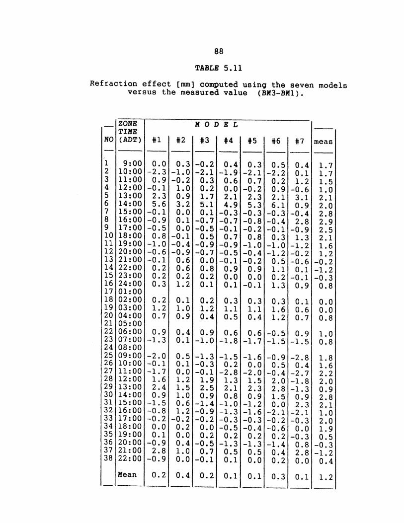
88

TABLE 5.11

Refraction effect [mm] computed using the seven models versus the measured value (BM3-BM1).

NO

1 2 3 4 5 6 7 8 9 10 11 12 13 14 15 16 17 18 19 20 21 22 23 24 25 26 27 28 29 30 31 32 33 34 35 36 37 38

ZONE TIME (ADT)

9:00 10:00 11:00 12:00 13:00 14:00 15:00 16:00 17:00 18:00 19:00 20:00 21:00 22:00 23:00 24:00 01:00 02:00 03:00 04:00 05:00 06:00 07:00 08:00 09:00 10:00 11:00 12:00 13:00 14:00 15:00 16:00 17:00 18:00 19:00 20:00 21:00 22:00

Mean

i1 --

0.0 -2.3 0.9

-0.1 2.3 5.6

-0.1 -0.9 -0.5 0.8

-1.0 -0.6 -0.1 0.2 0.2 0.3

0.2 1.2 0.7

0.9 -1.3

-2.0 -0.1 -1.7 1.6 2.4 0.9

-1.5 -0.8 -0.2 0.0 0.1

-0.9 2.8

-0.9

0.2 --

M 0 DEL

i2 i3 +4 -- -- --

0.3 -0.2 0.4 -1.0 -2.1 -1.9 -0.2 0.3 0.6 1.0 0.2 0.0 0.9 1.7 2.1 3.2 5.1 4.9 0.0 0.1 -0.3 0.1 -0.7 -0.7 0.0 -0.5 -0.1

-0.1 0.5 0.7 -0.4 -0.9 -0.9 -0.9 -0.7 -0.5 0.6 0.0 -0.1 0.6 0.8 0.9 0.2 0.2 0.0 1.2 0.1 0.1

0.1 0.2 0.3 1.0 1.2 1.1 0.9 0.4 0.5

0.4 0.9 0.6 0.1 -1.0 -1.8

0.5 -1.3 -1.5 0.1 -0.3 0.2 0.0 -0.1 -2.8 1.2 1.9 1.3 1.5 2.5 2.1 1.0 0.9 0.8 0.6 -1.4 -1.0 1.2 -0.9 -1.3

-0.2 -0.2 -0.3 0.2 0.0 -0.5 0.0 0.2 0.2 0.4 -0.5 -1.3 1.0 0.7 0.5 0.0 -0.1 0.1

0.4 0.2 0.1 -- -- --

45 +6 -- --

0.3 0.5 -2.1 -2.2 0.7 0.2

-0.2 0.9 2.3 2.1 5.3 6.1

-0.3 -0.3 -0.8 -0.4 -0.2 -0.1 0.8 0.3

-1.0 -1.0 -0.4 -1.2 -0.2 0.5 0.9 1.1 0.0 0.2

-0.1 1.3

0.3 0.3 1.1 1.6 0.4 1.2

0.6 -0.5 -1.7 -1.5

-1.6 -0.9 0.0 0.5

-2.0 -0.4 1.5 2.0 2.3 2.8 0.9 1.5

-1.2 0.0 -1.6 -2.1 -0.3 -0.2 -0.4 -0.6 0.2 0.2

-1.3 -1.4 0.5 0.4 0.0 0.2

0.1 0.3 -- --

i7 me as --

0.4 1.7 1.7 1.5. 1.0 2.1 2.0 2.8 2.9 2.5

0.1 1.2

-0.6 3.1 0.9

-0.4 2.8

-0.9 1.

-1. -0. -0.

0. -0.

0.

o. 0. 0.

0. -1.

-2. 0.

-2. -1. -1. 0. 2.

-2. -0.

0. -0.

0. 2. 0.

0.

3 2.1 2 1.6 2 1.2 6 -0.2 1 -1.2 1 -0.3 9 0.8

1 0.0 6 0.0 7 0.8

9 1.0 5 0.8

8 1.8 4 1.6 7 2.2 8 2.0 3 0.9 9 2.8 3 2.1 1 1.0 3 2.0 0 1.9 3 0.5 8 -0.3 8 -1.2 0 0.4

1 1.2

model #1 model #2 model #3 model #4 model #5 model #6

·model #7 measured

model #1 model #2 model #3 model #4 model #5 model #6 model #7 measured

model #1 model #2 model #3 model #4 model #5 model #6 model #7 measured

89

TABLE 5.12

Correlation Coefficients Matrices

MODEL #1 #2 #3 #4 #5 #6 #7

1 0.89 1 0.96 0.89 1 0.93 0.94 0.92 1 0.95 0.94 0.95 1.00 1 0.88 0.96 0.87 0.97 0.97 1 0.79 0.78 0.77 0.75 0.75 0.74 1 0.50 0.42 0.56 0.48 0.49 0.41 0.36

a: gravel-grass (BM1-BM2) line

1 0.89 1 0.97 0.89 1 0.96 0.94 0.92 1 0.97 0.94 0.95 0.99 1 0.91 0.98 0.89 0.97 0.97 1 0.81 0.84 0·. 79 0.82 0.82 0.82 1 0.52 0.71 0.60 0.56 0.59 0.67 0.58

b: grass-asphalt (BM2-BM3) line

1 0.74 1 0.94 0.77 1 0.93 0.68 0.91 1 0.94 0.68 0.95 0.99 1 0.86 0.79 0.92 0.90 0.92 1 0.38 0.10 0.18 0.38 0.34 0.25 1 -.10 -.10 -.04 -.05 -.02 .02 -.03

c: asphalt-gravel (BM3-BM1) line

measur.

1

1

1

6

4

,...., 2

~ .........

.jJ 0 () Q)

4-1 4-1 ~

~ -2 0 ·n .jJ C)

ctl 1-1 -4

4-l Q)

0::

-6

-o 0

t!l

·,

I .1 II

12:00

I' I 1 I I

\ i \.../

I ' . \_/

20:00

I I I ._I I

/' ·. .

\ I . ' './'

-....· I

I I I \ · . ./

04:00

.~.' . /. \

I

I I

1

1

12:00

I ' I I

Zone LEGEND• o-El--a Me115ured ···---· Model #I ----- Model #2 --- Model #3

Figure 5.5:

t-1odel #4 ·--- Model #5 -----· Model #o ----Model

Refraction effect computed using the seven models versus the measured value for BM1-BM2.

#7

.-. .. .. .. .', \ \ J \ ',

I '

~ -o- ~ \: . I

~~-~\~ ,, .. ~

2o:oo Time (h]

1.0 0

,....., 6 6

...., 0 (!)

1.1-l 1.1-l J;:.J

~

6

4

0

0 -2 ·~ ...., 0 cO ~

~ (!) -4

~

I I I

·6-:J \/

' I I

.' I

(', . I

----. ' -,

,.\ I \ ,"' \ ... __ .... , 1 I, ·, I A;'" \

i X ;'·-:... . \ fr...:\ //. \ \ I I I . \

\ I/, ' \ ' \ I • ~ ~' \'\ ' "' I .-, I ' • ,., ~ h / ' ' ~-, '

.: ''.;~ ' "\h----..;;: \\ ~' , \ \' ' _, \• --- ' .: (! \ ~- ~ - \ \.; \ •h ' "' ,?" .o-., \ . •

)., f..t!l·-\c~ 'l!l., \'\..;.. ~ -p~-; . -'' I a./ '19. ·' : I~J ·" I

'" 1 ' \. ~.; / \_,

. I •

-6~------~------~-----~~----~--------~-------~------~------~------~ 0 12:00

LEGEND•

20:00 04:00 12:00 20:00 Zone Time [h)

o-EJ-<3 Me~5ured Model #4

Model #l Model #5

Model #2 11odel #6

Model #3 Model #7

Figure 5.6: Refraction effect computed using the seven models versus the measured value for BM2-BM3.

\0 .....

~

~ ......

+" () Q) ~ ~

ril

a 0

•.-i ...., ()

4

2

0

10 -2 >-! ~ Q)

ex;

-4

-E>

<3·-0·. 'q

12:00

I 1 19. I I •

I lll.

I' I I

'o •.

20:00 04:00

\

I

''\ G:l\ , ' I ~

/j':~' : I ',I , •• .-. r~·~\: 1 m P ~ ~ ·• . '• I .'

,' \ I •\ / ,.a.. .. -.,.- .... · '{ '\ ~ .. ' '0 ,, .... ,, ''T:J . ., : ~..... I \

I

I \ I

12:00

'-\..1 I 1 • 1 I

\ I \ I ' I

\' \ : :f,,l ' ~ \ li'r:l

I \~ \ 'I 'f/1 ~.:._. •I

''.Jill " t I v,

Zone 20:00

Time [h) LEGEND! D·EJ·-!3 Measured • • · • · •· Model #l ----- Model #2 ---Hodel #3

Figure 5.7:

Model #4 ·-·- Model #5 ··-··· Model #6 ----Model #7

Refraction effect computed using the seven models versus the measured value for BM3-BM1.

\0 N

93

5.5 Computed Versus Measured Refraction Effect

5.5.1 Tests on 20 June ~

The first test was performed on 20th of June as a

preliminary observation preparation for the long term tests.

Only the height difference between BMl and BM2 was measured

repeatedly for four hours from 10:20 to 14:30. Table 5.13

shows the discrepancies between the geodetic height

differences and UNB method trigonometric height differences.

TABLE 5.13

Preliminary test measurements using UNB trigonometric method at South-Gym area from BMl to BM2

Geod. - Trig. [mm] REMARKS

mean cloud -LOCAL 2.lm 3.5m of 2 cover

NO TIME tar tar tar \ condition -

1 10:25 0.1 -1.9 -0.9 50 Sunny 2 10:45 0.5 -1.2 -0.4 50 Sunny 3 11:02 1.9 -0.4 0.8 50 Sunny, Windy 4 11:16 -0.3 -1.5 -0.9 70 Windy 5 11:32 -1.0 -1.8 -1.4 90 Windy 6 11:54 -3.6 -2.2 -2.9 100 Breeze 7 12:12 -2.1 -1.0 -1.5 100 Windy 8 12:30 -0.1 -1.1 -0.6 75 Sunny periods, windy 9 13:01 -1.6 -2.0 -1.8 50 Sunny periods, windy

10 13:15 0.7 0.2 0.5 50 Sunny periods, windy 11 13:47 -4.1 -3.9 -4.0 75 Windy 12 14:00 -2.2 -2.4 -2.3 75 Windy 13 14:13 -0.6 -1.2 -0.9 75 Windy

Mean -0.95 -1.57 -1.25 s. D. 1. 72 1.01 1.31

94

The day on which the observations were carried out was

reported as windy. In a moderatly windy day of summer, the

Obukhov length defined in section 3.1.2 is usually longer

than 30m (see e.g. Greening, [1985]). The results of the

first three rows show positive values for the lower targets

and negative values for the heigher targets. This was first

thought to be due to the inversion of the temperature

gradient, but later it was found that the magnitude of the

refraction effect can change sign with elevating line of

sight regardless of the sign of the temperature gradients.

On a windy day, region II (the middle region of thermal

stability, see section 3.1.3 for more detail) extends

usually to more than 30 m (one Obukhov length) and according

to theories (see e.g. Webb, [1984]), inversion of

temperature, on a windy day of summer with light cloud

cover, cannot appear below this range. However on calm

days, when the horizontal movement of air is less than 2

m;s, one may expect momentarily inversion of temperature

gradients within the first three metres of the atmospheric

layer. But, this does not necessarily mean that the lower

targets will result in a sign of refraction effect different

from the results of the higher targets (see also section

5.3.6).

The meteorological

were: air temperature

measured distances, and

observations done on 20 June 1985

and pressure for correcting the

a record of cloud cover and wind.

95

No temperature gradient was measured, therefore the

magnitude of refraction effect using the meteorological data

could not be obtained for the first test. For all other

tests the wind velocity and direction, temperature gradient,

atmospheric pressure, humidity, and temperature of the

ground surface were measured and cloud cover was recorded.

Although all this information was useful for understanding

the changes of atmospheric condition and if possible their

correlation with the refraction error, only the temperature

gradient was used to compute the magnitude of refraction

effect.

5.5.2 Tests Qn li July ~

The second test was carried out on 19 July 1985. It was

supposed to continue for 24 hours, but due to unfavourable

weather conditions it was interrupted after 13 hours of

continuous observations. The height differences between BM1,

BM2 and BM3 were measured repeatedly over the whole 13-hour

period.

Tables 5.14, 5.15 and 5.16 show the discrepancies

between the height differences obtained using precise

geodetic levelling and using the UNB-method. These

discrepancies can be interpreted as mostly due to the

refraction effect by assuming the results of geodetic

levelling as being errorless.

96

TABLE 5.14

Discrepancies between the results obtained using trigonometric height traversing and geodetic levelling for

BMl to BM2.

Geod. - Trig. [mm] REMARKS

mean cloud LOCAL 2.lm 3.5m of 2 cover

N 0 TIME tar tar tar ' condition

1 11:13 -0.1 -0.9 -0.5 75 2 12:09 -2.0 0.5 -0.7 100 Fair 3 13:24 -1.4 -2.7 -2.0 50 Windy 4 14:54 -2.7 -2.0 -2.3 75 Windy, little rain 5 15:49 -3.6 -1.2 -2.4 100 Little wind 6 18:05 -1.7 -1.5 -1.6 100 7 18:56 -2.4 -0.8 -1.6 100 8 19:31 -0.8 -1.0 -0.9 100 9 20:09 -2.6 -0.3 -1.5 100

10 21:56 -1.7 -2.2 -1.9 After a period of rain 11 22:47 -1.9 -0.7 -1.3 Cloudy 12 23:25 -0.7 -0.7 -0.7 Cloudy

Mean -1.80 -1.13 -1.45 s. D. ±0.97 ±0.87 ±0.64

Since the profile of surface on the fore-sight of one

line is the same as the back-sight of the other, one can

expect that over a long period the misclosure of the three

height differences would be near zero. The mean misclosure

for the lower targets is -0.03 mm i.e. as expected. But

the mean misclosure for the higher targets is -0.85 mm which

is considered as too large.

Column 2 of Table 5.15 shows that the mean discrepancies for

target 3.5 m is a negative number. This value was expected

97 •

TABLE 5.15

Discrepancies between the results obtained using trigonometric height traversing and geodetic levelling for

BM2 to BM3.

Geod. - Trig. [mm] REMARKS

mean cloud LOCAL 2.1m 3.5m of 2 cover

N 0 TIME tar tar tar % condition

1 11:31 -1.5 -1.8 -1.6 75 shimmers on BM3 2 12:28 -1.6 -2.7 -2.1 25 Shimmers on BM2. 3 14:00 2.2 -0.8 0.7 50 Windy 4 15:16 0.3 -0.5 -0.1 100 Windy, little rain 5 16:04 0.0 -0.1 -0.1 100 Little windy 6 18:29 0.3 -0.1 0.1 100 7 19:07 0.8 0.4 0.6 100 8 19:41 2.0 0.7 1.3 100 9 20:21 2.3 1.7 2.0 100

10 22:18 1.1 -0.5 0.3 100 After a period of rain 11 22:59 0.7 0.6 0.7 100 Cool 12 23:35 0.6 0.5 0.5 100 Little windy

.Mean 0.60 -0.22 0.19 S. D. ±1.26 ±1.18 ±1.13

to be positive. The computed refraction using the profile of

the lines and measured temperature gradient in Table 5.17,

indicates positive mean values for both targets.

This can be explained by using Figure 5.8 When

RB-RF > 0 then AHG-AHT < 0 and when RB-RF < 0 then

AHG-AHT > 0. The first case had mostly occurred for the

lower targets and the second case for the higher targets.

The temperature gradient on the grass field close to the

ground (0.3 m to 1.2 m) is larger in magnitude than the

98

TABLE 5.16

Discrepancies between the results obtained using trigonometric height traversing and geodetic levelling for

BM3 to BM1.

Geod. - Trig. [mm] REMARKS

mean cloud -LOCAL 2.1m 3.5m of 2 cover

NO TIME tar tar tar \ condition -

1 11:49 1.5 1.9 1.7 75 Breeze 2 12:46 2.7 -0.3 1.2 0 Sunny 3 14:17 3.1 1.8 2.4 95 4 15:36 1.2 0.4 0.8 100 Little rain & wind 5 16:32 1.7 0.9 1.3 100 Little windy 6 18:43 -0.2 0.6 0.2 100 7 19:19 0.2 -0.1 0.1 100 8 19:59 0.4 -0.4 0.0 100 9 22:35 1.1 0.0 0.5 100 After a period of rain

10 23:12 0.8 0.0 0.4 100 11 00:05 0.4 0.7 0.5 100

Mean 1.17 0.5 0.83 S. D. ±1.03 ±0.79 ±0.75

temperature gradient over asphalt close to the ground, and

it is smaller when going higher above the surface (1.2 rn to

4 rn). This may explain the different signa of values, but

cannot explain the large miaclosure of -0.85 mm for the

higher targets. However, this rather irregular misclosure

was not repeated in the three other cases and was always

nearly zero.

99

TABLE 5.17

Computed refraction using measured temperature gradient

Computed Refraction [mm)

LOCAL BMl to BM2 BM2 to BM3 BM3 to BMl NO TIME 2.1m 3.5m Mean 2 .1m 3.5m Mean 2.1m 3.5m Mean

-- -- -- -- -- -- -- -- --1 11:00 2.4 1.6 2.0 2 12:00

-2.8 -1.6 -2.2 -0.2 -0.4 -0.3

3 13:00 -3.9 -3.6 -3.7 4.9 4.5 4.7 -1.6 -1.3 -1.4 4 14:00 5 15:00 -1.2 -0.2 -0.7 1.7 1.1 1.4 -0.8 -1.2 -1.0 6 16:00 1.9 1.3 1.6 7 17:00 0.0 0.3 0.1 0.2 0.2 0.2 -0.5 -0.7 -0.6 8 18:00 0.2 0.2 0.2 9 19:00 -1.0 -0.7 -0.9 0.7 0.5 0.6

10 20:00 -1.0 -0.4 -0.7 0.1 -0.4 -0.1 0.8 0.6 0.7

Mean -0.65 0.83 -0.33 s. D. +1.84 +2.11 :t0.85

100

6HG height difference using geodetic levelling 6HT height difference using the leap-frog

trigonometric method

6H ~ 6HG = 6HB + 6HF 6HT = 6HB + RB + 6HF - RF

= 6HG + (RB - RF)

I) If (RB - RF) > 0

II) If (RB - RF) < 0

THEN

THEN

(6HG - 6HT) < 0

(6HG - 6HT) > 0

6HF

Figure 5.8: Back- and fore-sight magnitude of refraction difference

5.5.3

The third test survey in the South-Gym area started at

9:43 on 23 July 1985 and continued to the next day until

23:50 for a total of 38 hours of continuous observations.

The temperature gradient of air was measured during the

entire test period. Knowing the profile of the lines and

101

using equations (3.66) and (3.67), the refraction effect for

all three lines was computed for one hour intervals. Figure

5.9 shows:

1. The measured refraction effect which is the

discrepancy between the height difference determined

using geodetic levelling and the results obtained with

the UNB-method of trigonometric height traversing

(6HG- 6HT).

2. The computed refraction at one hour intervals using

the observed temperature gradients.

The error bars in this figure are based on the precision of

the observations and they have been increased to take into

account other errors (this will be briefly discussed in

section 5.3.8.).

The correlation between the two can be seen in Figure

5.9 parts a and b, and the correlation is more pronounced in

the latter for BM2 to BM3. A fitted linear regression line

(the solid line) in Figure 5.10 has small deviations from

the expected hypothetical regression line (the dashed line:

mr = cr). This figure shows the measured refraction effect

against the computed refraction effect for the line BM2-BM3.

The relationship between the measured, mr, and computed

refraction, cr, is defined by the regression equation (the

solid line in Figure 5.10):

mr = 0.3 + 1.2 cr (5.12)

102

with correlation coefficient, r = 0.60 • At the 1% level

of significance Ho : r = 0 is rejected and thus Ha r ~ 0,

i.e. correlation exists, can be accepted (for details of the

test see section 5.4.4). This is almost the same for the

line BM1-BM2. The lowest correlation exists between the

measured and the computed refraction effects for the line

BM3-BM1 (see Table 5.12).

In order to investigate the difference of measured and

computed refraction we may consider the lines from the

instrument station to the bench marks separately. A good

assessment of the refraction computation over each ground

surface is also possible by examining them individualy.

The refraction angle can be found by detecting the

neutral condition (see section 3.1.2) from temperature

measurements. Figure 5.11 depicts the approximate time of

neutral condition for different sufaces and elevations, i.e.

when the periodic temperature gradient crosses the zero

line. Figure 5.12 shows the fluctuations of observed

vertical angles to the lower targets. Using these graphs and

considering the corresponding time of neutral condition when

the refraction effect is expected to be almost zero, the

fluctuation around this zero point is mostly because of

refraction and can be computed simply by subtracting the

angle observed at neutral condition time from all other

corresponding measured vertical angles and assuming the

difference is the angle of refraction. The angle of

103

m: j I computed

t measured

2

4

e 1 1 ~ -2 I. ! I ~ -· II I ~ I ~ 0 ~

"-' 0 m ~

4-l <l) o:;

12:00 20:00 04:00 12:00 20~00

Zone Time [h)

b

Figure 5.9: Measured refraction effect versus the computed value. a. BM1-BM2, b. BM2-BM3 and c. BM3-BM1.

104

4

~ • e 2 • :& . e ~

·~ • •

~ 0 • ~ • •• • ~ • ~ • ro • ~ • m -2 • • • ~ e

-4

-4 -2 0 2 4

computed [mm]

Figure 5.10: The measured refraction effect [mm]. The discrepancies of height difference determined by

trigonometric height traversing and geodetic levelling for BMl-BM2 line versus the computed refraction error for the same line. The dashed line is the hypothetical regression

line, and the solid line represents the actual linear regression.

refraction found in this way is as precise as the measured

vertical angle, i.e. about 0.6" (see section 5.3.8);

however, its accuracy can be lower because of the bias

introduced due to the uncertaintity for detecting the

neutral conditon or the zero refraction angle time.

This angle of refraction is converted to linear

refraction and compared with the computed refraction for all

three lines in Figure 5.13 • In all three plots the strong

105

correlation between the two computed and measured refraction

effects can be seen. These plots are prepared for the mean

corresponding values of the two targets.

Figure 5.14 gives the linear correlations which exist

between computed and measured refraction effects. Table

5.18 gives the correlation coefficient, linear regression

equations relating the computed to the measured refraction

effect, and at the 1% level of significance the null

hypotheses that there is zero correlation between the

measured and the computed refraction effect (Ho : r = 0).

In Table 5.18, the regression equations show that the

computed refraction effect, cr, is too large compared to the

measured refraction effect, mr. Specifically over asphalt,

the measured refraction effect is more than four times

smaller than the computed one. There are two possible

explanations of why the results of asphalt are so different

from the other two surfaces:

1. The site chosen to make the temperature gradient

measurements was too close to the ground covered by

gravel (about 2 m) and was not characteristic of the road

on which the line of sight to BM3 was extended. The

reason for choosing that spot was the lack of proper

transportation to move the equipment from one site to

another.

2. The wind was blowing almost in the direction of the

line of sight to BM3. According to Webb [1968] this can

-0.8

E 0.4 ' u

0. 0 -1------

-0.4 ·._:

106

a

· ....

· ... ·

-... -·

c -0.6~--~--~---r--~--~--~~--.---~--~---r-

12:00 20:00 04:00 12:00 20:00

Zone Time [h]

----- l.5 2 2.5 3

Height Above the Ground (m]

Figure 5.11: Fluctuations of point temperature oradient a. gravel, b. grass and c. asphalt.

Ul 17 G)

...... ~ c:: «3

......

107

,,

a

! 4i' \f!\A . . I~A~~l ~ 39'J \; ~~~ \ . ~ \) ~~\ \ 0

~ '• 0 36

b

I • 12:00 20:00 04:00 12:00 20:00

Zone Time [h]

Figure 5.12: Fluctuations of observed vertical angles a. BMl (gravel), b. BM2 (grass), and c. BM3 (asphalt).

,....... e e

mm

-4

4

2

-4

" (

. . : . . . .. .. .

. ' . ' . ' "

12:00

..

108

{a) Gravel

f··'\ .. ;. . . ' ·. ' I . .

' .. .,

','· .... .. . .. •

(b) Grass

: ,'. ~ .....

computed

measured

. · .

... . . .. '.

-..'I I ,, (c) Asphalt

,·. I r I I . ' . '' '

20:00 04:00 12:00

Zone Time [h]

~ .. I\ . . . '

,' ~~ ,•

·' _..:

20:00

Figure 5.13: Computed refraction effect versus the measured value. a. IS-BMl (gravel}, b. IS-BM2 (grass)

and c. IS-BM3 (asphalt}.

109

result in lower refraction effect than the expected

(computed) value. Other than the wind direction, during

the day, the traffic on the road could also result in a

mixing of the atmosphere and a reducing of the effect of

refraction.

be noticed

The lower refraction effect over asphalt can

from the small fluctuations of the vertical

angle in comparison to the other two in Figure 5.12

It was previously mentioned that, as can be seen in

Figure 5.9 c, the discrepancies between the geodetic

levelling and trigonometric height traversing of BM3-BM1

versus the computed refraction have very weak correlation

(Table 5.12). Using the regression equations in Table 5.18

for asphalt and gravel, the computed refraction was

corrected according to these two equations, given cr as

computed then mr will be the corrected refraction effect. A

significant improvement in the correlation coefficient was

found between the two after the corrections were made. The

correlation coefficient improved to 0.68 .

The significant correlations of the two measured

refraction effects (either derived from the angle of

refraction or from discrepancies between geodetic and

trigonometric methods of height differnce determination)

against the computed refraction is mostly due to the

detailed knowledge that we have about the surface profiles

and to the long term temperature gradient measurements.

110

• (a) Gravel 4

(b) Grass • • 4

2 • 2 • •

.--. g 0 e • e • 0 • '0 '0 Q)

-2 (I) .... .... ==' ::s -2 0. 0. e • e 0

0 -4 0 • • 0 •

-4

-6

-4 -2 0 2 -4 -2 0 2 measured [mmJ measured [mm)

4 (c) Asphalt

2 • • • • e • e •

0

'0 Q) .... -2 • ::l p. e 0 0 • -4

•

-4 -2 0 2 measured [mm]

Figure 5.14: Linear correlation between the computed and measured refraction error.

a. IS-BMl (gravel), b. IS-BM2 (grass) and c. IS-BM3 (asphalt).

111

TABLE 5.18

t-test on the significance of the correlation coefficients

* Surface from Corr. Regression Equat. H

IS Coef. t > t to 33,0.005 -- --

** gravel BMl 0.87 mr= -0.13+0.51 cr 10.7 > 2.75 R

grass BM2 0.87 mr= -0.36+0.40 cr 10.7 > 2.75 R

asphalt BM3 0.66 mr= -0.31+0.23 cr 5.3 > 2.75 R -- --

* t = and the table values for t at 0.01

and 0.05 level are: t = 2.75 and t = 2.0 33,0.005 33,0.025

** Ho: r = 0 is rejected and Ha: r ~ 0 is accepted.

Although the correlations are significantly high, the

computed refraction error cannot be trusted in practical

work, since it is not accurate enough and may cause too

large corrections for lines longer than 100 m in

trigonometric height traversing (see section 4.2.3).

However, the results proved that simulations of the

refraction effect in trigonometric height traversing over a

known profile with known temperature gradient along the

profile, can be very realistic, and useful information may

112

be extracted from such simulations. For more details see

Chapter 6.

5.5.4 Tests on 12 ~ ~ and estimation Qf standard deviatipn of vertical angle measurements

The last test at the South-Gym area was carried out

using two independent theodolites separated by about 2 m on

29 July. The main purpose in making these measurements was

to get sufficient data to estimate the actual precision of

trigonometric height traversing without the influence of the

refraction error. Two electronic theodolites were used, and

the observations were taken independently but not

simultaneously, for a duration of 5.5 hours starting at

11:45 ending at 17:07. Since the measurements were not

synchronized in time, their differences were affected by

short-term fluctuation of temperature gradient. Thus, one

may expect higher precision than what has resulted from this

experiment.

Estimation of the standard deviation of one ~H is given

by Chrzanowski [1985]

a= [ ~ i

where n

2 d.AH

i

is

I 2n

the

] -1/2

(5.13)

number of observations (usually

simultaneously taken) and d~H is the difference of the two

height traversings. An average standard deviation of

113

0.79 mm was found that corresponds to a standard deviation

of 0.58" for a zenith angle measured in four sets with

sight lengths of 200 m. The bars plotted in Figure 5.9 were

computed considering the above estimated standard deviation

as well as the contribution of other sources of errors such

as a change of the height of targets due to the expansion or

contraction of the rods, non-verticality of the rods, and

errors in the distance measurements. These errors are

discussed in detail by Chrzanowski [1984] and Greening

[1985].

Figure 5.15 shows the following refraction errors:

1. measured using electronic theodolite #1;

2. measured using electronic theodolite #2;

3. computed and corrected according to

presented in Table 5.18 and temperature

measured on 29 July 1985;

4. extracted from measurements carried out

1985 and corrected using equations given in

and

equations

gradient

in 23 July

Table 5.18;

5. extracted from measurements carried out in 24 July

1985 and corrected using equations given in Table 5.18 •

Considering the errors involved in both measuring and

computing the refraction effect, one can see that the above

five groups of values agree closely. This can be an

indication that the equations in Table 5.18 are useful

{only for these particular lines) and can improve the

r-o

e e ........

~ 0 G) ~ ~

tll

s::: 0 "M +.J

2

0

-2

2

• 0

• 0 0 0

0 0

8. 0

8.

114

1::. 8.

0 0

A: 1

0:2

0:4

o:s

~

1::.

08 ~

• 0

0G 8. 6 08. 0 0

0 t::.,p 0

0

0

0 0+-----~~=----------=------------~--~~~r-------~-~ 0 0 6. •6 06 0 S ~ 0 0 • 0 ' 0

G) <b El 0 68 ~ -2 • . 6

[:] 0

6 0 0 0

2 0

6 08 8. f::::P

. 0 Q

0

-2

12:00

'0 8

"8 Q

0

14:00

Zone Time (h)

6 !:.:.. 0

08 0 0

16:00

Figure 5.15: Measured refraction error versus the computed value. a. BM1-BM2, b. BM2-BM3 and c. BM3-BM1 (a

key to this figure is given in section 5.5.4).

115

computed values. Also, it is

effect from one day to another

as the measurements are carried

of day over the same profile

conditions.

realized that the refraction

is almost the same, as long

out within the same portion

and under similar weather

5.5.5 Comments on South-Gym ~ surveys

The refraction effect is successfully estimated by

treating the measurements carried out durino (or near to)

the neutral condition time as free from refraction error.

The computed values using this procedure are strongly

correlated with the measured refraction effect, with

correlation coefficients of 0.78, 0.93 and 0.83 for lines

BM1-BM2, BM2-BM3 and BM3-BM1 respectively.

The computed refraction effect for individual lines

(i.e. from mid point to the three bench marks) is larger

than these estimated (previously called "measured" based on

detection of neutral condition) values. The over estimation

of the refraction effect can be due to insufficient

knowledge of the variablity of the temperature gradient

along the line of sight which could not be taken into

account. However, in the computation of a full line (i.e.

from one bench mark to another) the over estimations mostly

cancelled out (see equation (5.12)) , as expected.

The preferable times for observations durino clear days

are early in the morning, a short time after sunrise, and in

the afternoon, a short time before sunset.

116

Measurements to the higher target (at 3.5 m height) are

less affected by refraction, but this does not necessarily

always cause randomization of refraction error, although in

some of the cases the discrepancies listed in Tables 5.13,

5.14, 5.15 and 5.16 show a sian for lower targets (at 2.1 m

height) different from the higher targets.

5.5.6 Tests on QQ August ~

The final test survey was carried out on the Head-Hall

test line. A description of the line is given in section

5.2.2. The change in temperature at different heights from

the ground was measured using six temperature sensors. The

site for temperature measurements was selected at a spot

close to BM4, on asphalt about 0.3 m from the concrete

side-walk. 39 setups of measurements were carried out in

which, as in the South-Gym observations, each setup

consisted of two sets of zenith angle- and distance

measurements. Observations started at 12:15 and ended at

about 20:00 on 06 August 1985. Figure 5.16 shows:

1. The measured refraction effect which is the

discrepancy between the height difference

using geodetic levelling and

trigonometric method (~HG- ~HT).

results

determined

of UNB

2. The computed refraction at 15 minute intervals using

the observed temperature gradients.

........

~ 0 Q) ~ ~

t:z1

a 0

6

4

2

• 0

0 (.j

• 0

•

•

0

0 • 0 • G{:l. 0

~G e 0

c

117

•

0

0 •

0

•

•

0 0

• • 0

• 0

• • 0 •

0

•

0

o measured

• computed

• •• o c 0 •

0 0

• • •

0 0

(:)

• • 0

•

-~ 0

6 0 +---------------~~----------------------------~r,-~---­0

0

m 1-4 ~ Q)

0:: -2

0 v

•

14:00 16:00 18:00 20:00

Zone Time [h)

Figure 5.16: The discrepancies of height difference determined by trigonometric height traversing and geodetic levelling, between BM2 and BM4 at Head-Hall test line.

Applying the computed refraction effect to correct the

observed height differences generally improves the results.

It should be mentioned that the profile of the baseline was

well known and the temperature gradient was determined every

five minutes. The average of the measured refraction effect

(for the mean of the two targets) came out to be 2.2 mm and

the corresponding computed value is 2.7 mm.

Assuming that the last observation at 20:10 is free of

refraction error (since it is the closest possible

observation to the neutral

effect on back-sights

separatly. Table 5.19

refraction effect:

1. back-sight,

2. fore-sight,

118

condition time), the refraction

and fore-sights was obtained

shows the following values of

3. total of the above two (measured, tl),

4. AHG - AHT (measured, 12), and

5. computed.

The refraction effect on the back-sight is oscillating more

or less around the zero value and on fore-sight is always

less than zero as expected.

Excellent agreement exists

values (11 and 12 in Table

coefficient of 0.93 which

between the two measured

5.19) with a correlation

substantiates that the

measurements carried out during the neutral condition time

can be assumed as a reference (free from refraction error)

and then the refraction effect can be computed for other

measurements. The neutral condition can be detected by

measuring temperatures at different elevations above the

ground. In this case the profile of the line is not needed.

This method of neutral condition detection can be utilized

in precise measurements of monitoring the vertical movements

of large structures, such as dams.

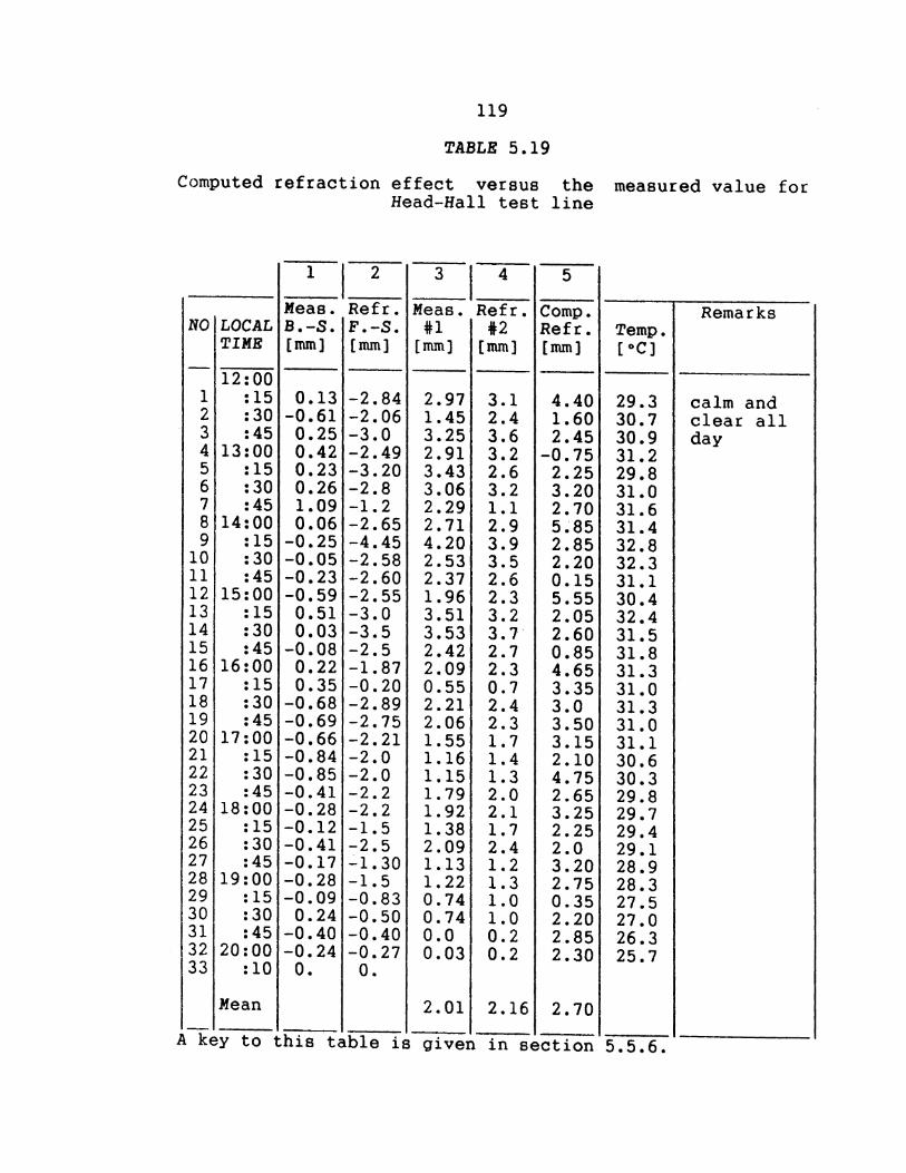
119

TABLE 5.19

Computed refraction effect versus the measured value for Head-Hall test line

NO

1 2 3 4 5 6 7 8 9

10 11 12 13 14 15 16 17 18 19 20 21 22 23 24 25 26 27 28 29 30 31 32 33

LOCAL TIME

12:00 :15 :30 :45

13:00 :15 :30 :45

14:00 :15 :30 :45

15:00 :15 :30 :45

16:00 :15 :30 :45

17:00 :15 :30 :45

18:00 :15 :30 :45

19:00 :15 :30 :45

20:00 :10

Mean

1 I 2

Meas. Refr. B.-s. F.-s. [mm] [mm]

0.13 -2.84 -0.61 -2.06 0.25 -3.0 0.42 -2.49 0.23 -3.20 0.26 -2.8 1.09 -1.2 0.06 -2.65

-0.25 -4.45 -0.05 -2.58 -0.23 -2.60 -0.59 -2.55 0.51 -3.0 0.03 -3.5

-0.08 -2.5 0.22 -1.87 0.35 -0.20

-0.68 -2.89 -0.69 -2.75 -0.66 -2.21 -0.84 -2.0 -0.85 -2.0 -0.41 -2.2 -0.28 -2.2 -0.12 -1.5 -0.41 -2.5 -0.17 -1.30 -0.28 -1.5 -0.09 -0.83

0.24 -0.50 -0.40 -0.40 -0.24 -0.27

0. 0.

3 I 4 5

Meas. Refr. Comp. i1 42 Refr. Temp.

[mm] [mm] (mm] [oC]

2.97 3.1 4.40 29.3 1.45 2.4 1.60 30.7 3.25 3.6 2.45 30.9 2.91 3.2 -0.75 31.2 3.43 2.6 2.25 29.8 3.06 3.2 3.20 31.0 2.29 1.1 2.70 31.6 2.71 2.9 5.85 31.4 4.20 3.9 2.85 32.8 2.53 3.5 2.20 32.3 2.37 2.6 0.15 31.1 1.96 2.3 5.55 30.4 3.51 3.2 2.05 32.4 3.53 3.7 2.60 31.5 2.42 2.7 0.85 31.8 2.09 2.3 4.65 31.3 0.55 0.7 3.35 31.0 2.21 2.4 3.0 31.3 2.06 2.3 3.50 31.0 1.55 1.7 3.15 31.1 1.16 1.4 2.10 30.6 1.15 1.3 4.75 30.3 1. 79 2.0 2.65 29.8 1.92 2.1 3.25 29.7 1.38 1.7 2.25 29.4 2.09 2.4 2.0 29.1 1.13 1.2 3.20 28.9 1.22 1.3 2.75 28.3 0.74 1.0 0.35 27.5 0.74 1.0 2.20 27.0 0.0 0.2 2.85 26.3 0.03 0.2 2.30 25.7

2.01 2.16 2.70

A key to this table is given in section 5.5.6.

Remarks

calm and clear all day

Chapter 6

SIMULATIONS Qf REFRACTION ERROR IN TRIGONOMETRIC HEIGHT TRAVERSING

6.1 Simulation Alonq g Geodetic Levelling Line on Vancouver Island

In 1984 a number of levelling simulations were carried

out at UNB to assess the dependence of the refraction errors

on the profile of the terrain in extreme environmental

conditions. The simulations were helpful to understand the

cumulative influence of refraction error in trigonometric

height traversing. The influence of refraction in geodetic

levelling and trigonometric heighting were simulated along

an 82 km long simulated profile with an assumed average

temperature gradient. The results of these simulations are

reported in details by Chrzanowski [1984] and Greening

[1985].

A number of new simulations has been done by the author

with the same purpose as in previous simulations but using

actual levelling data. The new simulations have been

conducted along a line of actual geodetic levelling of

special order (the allowable discrepancy between independent

forward and backward levelling between bench marks is less

than +3 mm~K [Surveys and Mapping Branch, 1978], where K

is the distance between bench marks in kilometres). During

- 120 -

121

the geodetic levelling operations, temperatures were

observed at heights 0.5 m and 2.5 m in every set-ups. The

distances from the instrument to back- and fore-sight

levelling rods were measured using stadia cross hairs. The

geodetic levelling was carried out on Vancouver Island by

the Geodetic Survey of Canada, Department of Energy, Mines

and Resources Canada, Surveys and Mapping Branch. The

project started in late May 1984 and was finished in the

middle of October 1984. The simulations have been carried

out over a ~224 km line chosen from the above data . The

line is divided into two parts for forward and backward

levelling traverses:

line from to

#1 Forward 108.5 km Nanoose Bay Mervi1le #2 Forward 115.7 km Merville Kelsey Bay #3 Backward 115.5 km Kelsey Bay Merville #4 Backward 109.2 km Merville Nanoose Bay

Lines #1 and #4 are extended- totally over a flat terrain,

parallel to the southern shore-line of the Strait of

Georgia. Lines #2 and #3 pass partially over a hilly

terrain south of the Menzies, Kitchener and Hkusam mountains

with maximum height differences of about 300 m. The profile

of the line was generated for 10 m (or less) intervals

along the line based on measured stadia distances and height

122

differences of turning points. Assuming the slope of the

ground between two adjacent turning points as being

constant, every two adjacent turning points were connected

by a straight line and then the height of points with

maximum 10 m horizontal separation was interpolated along

the line. See Figures 6.2 to 6.5 for the profile of the

lines.

The actual accumulation of the refraction effect in

geodetic levelling has been computed and the simulation of

refraction accumulation in trigonometric height traversing

was done using the same temperature gradient and the same

profile.

6.1.1 Computation 21 the refraction error in geodetic levellina

The temperature differences measured during levelling

were used in Kukkamaki's formulae for refraction correction

using equation (3.19). This equation was simpilified by

Kukkamaki [1939a] to a form more convenient for computation

using a hand calculator

-5 2 Cr = 10 G . (S/50) . Ah . At (6.1)

in which,

5.94

[ 1 C+l C+1 c

200 ] G = --------- ----- ( 50 250 ) + 150 . c c c + 1

250 - 50 (6.2)

123

where, Ah = the levelled height difference in scale division

0.5 mm, and

~t = the measured temperature difference between 2.5

m and 0.5 m above the ground surface.

In equation (6.1), Kukkamaki assumes that the refraction

correction varies linearly with the height difference Ah,

and the measured temperature difference ~t.

In equation (6.2), c is the exponent in Kukkamaki's

model. Based on Hytonen's [1967] investigations, Kukkamaki

[1979], suggests that an average value of c = -0.1 with

corresponding G = 69.4 can be used in all circumstances

without causing any significant loss of accuracy. However,

the author assumed a constant value of -1/3 for c as in

equation (5.11), obtaining G = 80.5. For c = -1/3,

Cr = 0.07 mm and for c = -0.1, Cr = 0.08 mm can be found

assuming ~t = -0.25 oc, S = 50 m and ~h = 2 m.

Geodetic refraction was also computed using Remmer's

formula which is an adaptation of equation (3.19) given by

Kukkamaki [Remmer, 1980]

2 S dn

Cr = (----)( d2 ~h + 6 dt

d4

80

3 ~h ) (6.3)

where: dn/dt is given by equation (3.11), d2 and d4 are

the second and the fourth derivatives of Kukkamaki's

temperature function respectively which are

c-2 d2 = {C-1) C b z

124

and

c-4 d4 = (c-3) (c-2) (c-1) c b z

S is the sight length and ~h is the height difference for a

single set-up. All three equations (6.1), (3.19) and (6.3)

were used to compute the refraction effect in geodetic

levelling along the above lines and as can be seen in Figure

6.1, the answers came out to be in close agreement. The

figure shows the effect of refraction in geodetic levelling

along the line 43. The mean of the three is used for

comparison with the simulated refraction effect in the

trigonometric methods (see e.g. Figura 6.2 to 6.5).

6 .1. 2 Refraction error in trigonometric height traversing

The refraction effect in trigonometric height

traversing was computed using equation (2.13)

1 I Cr = k (S - X) dx = (6.4)

R R

in which I is given by equation (4.1). For a special case,

when

6 = 6 = S = 1 2

= 8 I

n

this can be written as

125

8 I = k s + k 8 (S - S)+k 8 (S - 2 B)+ . . . . .

1 2 2 3

1 2 ••••• + k 8 (6.5)

2 n

where

502.7 p k = ------- [ 0.0342 + (dt/dz) ] , (6.6)

i 2 i T

-4/3 dt/dz = (-1/3) b z (6.7)

and S is the sight length divided into n equal subsections

of s (S = n s).

6 .1. 3 Results of simulations

Figures 6.2 to 6.5 show the results of four

simulations. The starting heights of the profiles were

chosen arbitrarily. As can be seen, the geodetic levelling

refraction effect is highly correlated with the profile of

the levelling route, but, fluctuates within the limits of

special order of Canadian accuracy specifications. On the

other hand, the refraction errors in trigonometric height

traversing are not correlated with the profile of the route.

They are highly dependent on the clearance and the length of

the line of sight as it would be expected. To show this

dependency, one can keep the maximum length of sight

126

unchanged while changing the clearance. In all four lines

the error of refraction will be reduced by increasing the

clearance, where the number of observations will be

increased as well. Conversely in most of the cases, keeping

the clearance unchanged while increasing the sight length,

will result in a higher refraction error, and decreasing the

sight length will help to decrease the refraction effect.

Many more simulation results were obtained for

different cases of the sight lengths and the ray clearances.

By inspection of these cases and those presented in this

thesis, it is substantiated that if the lines of sight in

the leap-frog method are less than 150 m with the ray

clearance greater than 1 m, the refraction effect is within

the limits of the Canadian specifications for the first

order levelling. The Canadian specification for first order

and for one-way levelling is given by Chrzanowski [1984] in

terms of standard deviation as U ~ 2.0 mm~K, where K is in

kilometres. The line of sight should be less than 250 m for

the clearance of 1 m in the case of reciprocal method. It

should also be mentioned that the height of 2 m for the

instrument is assumed for all the results shown in here.

The height of instrument, according to the author's

experience is usually more than 2.2 m in motorized

trigonometric height traversing. A considerable improvement

is noticed in the results of simulations whenever a height

of larger than 2.2 m for the instrument is assumed.

127

6.2 Simulation of the Refraction Error Using other Values of Temperature Gradient Measurements

According to the measured temperatures (at height 0.5 m

and 2.5 rn above the ground), the weather condition during

the levelling in Vancouver Island was quite mild. To

investigate the changes of weather, one can look at the

changes of sensible heat flux, H along the route of the

above levelling lines (#1 to #4). The H can be estimated

from the temperature gradient profile in the middle region

under unstable conditions, using equation (3.32) and

neglecting the adiabatic lapse rate r = 0.0098 (see equation

(3.23));

dt 2/3 -4/3 = -0.0274 H z (6.8)

dz

Equating the right hand sides of equations (6.7) and (6.8),

H can be written in terms of b (see section 3.1.5)

H = [ b

(6.9) 0.0822

in which, b is given in terms of ~t according to equation

(3.4)

c c b = ~t I ( 2.5 - 0.5 ) (6.10)

where c = -1/3 and ~t is the temperature difference

between lower (at 0.5 m height) and higher (at 2.5 m height)

sensors.

128

Figure 6.6 shows the variations of sensible heat flux

along the line i2 . The negative values may be slightly

different from those depicted in this figure, since the

negative values reflect the stable condition and they have

to be computed with the help of the corresponding equation

(3.33) or (3.34). Table 6.1 shows the averaged

coefficient b and its corresponding H values along the four

levelling lines. Table 6.2 and 6.3 show other examples of

these values in other parts of Canada (Fredericton, N.B.)

and in the United States. For example in Fredericton,

according to meteorological obsevations carried out, one can

expect higher H and b values during the summer than those

from Vancouver Island.

TABLE 6.1

Average ~t, b and H along the levelling routes

Line ~t b H

-2 [oC] [W m ]

il -0.39 0.75 28 i2 -0.28 0.53 17 i3 -0.37 0.71 25 i4 -0.36 0.69 24

MEAN -0.35 0.67 23.5

129

TABLE 6.2

Average ~t, b and H in Fredericton, N.B.

Date Ground ~t b H Time Remarks 1985 Cover ** *

-- -- --Jul-19 gravel -0.6 1.15 52 10:25-19:59 partially cloudy Jul-19 grass -0.3 0.57 18 10:45-19:35 partially cloudy Jul-19 asphalt -0.7 1. 34 66 10:10-20:32 partially cloudy Jul-23 gravel -0.7 1.34 66 10:10-18:20 mostly sunny Jul-23 grass -0.6 1.15 52 09:30-18:40 mostly sunny Jul-23 asphalt -0.7 1.34 66 09:50-19:00 mostly sunny Jul-24 gravel -0.8 1. 53 80 07:00-17:20 mostly sunny Jul-24 grass -0.7 1. 34 66 07:20-18:48 mostly sunny Jul-24 asphalt -0.7 1. 34 66 07:45-19:05 mostly sunny Jul-29 gravel -0.7 1. 34 66 12:10-17:10 partially cloudy Jul-29 grass -0.9 l. 72 95 11:30-16:30 partially cloudy Jul-29 asphalt -0.8 1.53 80 11:50-16:50 partially cloudy Aug-06 asphalt -0.7 1. 34 66 11:00-20:15 mostly sunny Aug-10 highway -1.0 1. 91 112 07:28-15:23 mostly sunny Aug- highway -0.7 1. 34 66 13:32-15:04 mostly sunny Aug-14 highway -0.9 1. 72 95 11:13-16:~5 mostly sunny Aug-15 highway -0.1 0.19 4 07:28-12:34 mostly cloudy Aug-15 highway -0.8 1. 53 80 13:06-15:36 partially cloudy

MEAN -0.7 l. 32 66 ------

** ~t is in oc 2

* H is in W 1 m

Applying the value b = 1.25 (see Table 6.2) in the

simulations along the Vancouver Island profile, one obtains

a set of results which can represent the refraction error in

the summer conditions of the Fredericton area.

Figures 6.7 and 6.8 show the simulation of refraction

error on the same profiles as in Figures 6.3 and 6.5 . In

these cases, the geodetic levelling needs to be corrected

130

TABLE 6.3

Average At, b and H along levelling routes in United States (after Holdahl [1982])

Num. Date Place of At b H

obs. -- --

December 1977 Gorman, CA 714 -0.75 1.43 73 Aug.-Sept. 1979 Gaithersburg, MD 838 -0.56 1.07 47 April 1980 Tucson, AZ 844 -1.03 1.97 117 May-June 1981 Palmdale, CA 1644 -1.29 2.47 165

-- --

for refraction. They also show that the dependency on the

value of b (or the magnitude of sensible heat flux, H) in

trigonometric height traversing is lower than for geodetic

levelling.

Refraction errors in both reciprocal and leap-frog

trigonometric height traversing were simulated along all 4

lines. In most cases the accumulation of refraction errors

in the reciprocal method is considerably lower than in the

leap-frog method. Looking at these simulations, one can see

that from refraction point of view, the reciprocal method is

more reliable than the leap-frog approach.

131

6.3 Simulation 2n the ~ Lines gt UNB

The refraction error in reciprocal trigonometric height

traversing was further investigated by simulation of this

error on the South-Gym and Head-Hall test lines (see section

5.2 for description of these test lines). The measured

temperature differences were used to compute the refraction

effect for both the leap-frog UNB-method which was actually

carried out, and an assumed reciprocal trigonometric height

traversing on the same profile. The line of sight in the

reciprocal method was selected to be

leap-frog. At the same time, it

reciprocal set-up on the extreme part

longer than for the

is tried to keep the

of the line where the

higher refraction effect is expected. For instance, in the

case of the Head-Hall test line, the reciprocal method

simulation was taking place for two points on the profile

which are closer to the center by 50 metres from each side

than the points used in the leap-frog measurements. The same

is true for the other three lines in the South-Gym area.

Figures 6.9 to 6.12 show the results of these

simulations. The starting heights of profiles were chosen

arbitrarily. In all four cases, the reciprocal method is

affected by the refraction error by about half the amount of

the leap-frog.

It was shown in Chapter 5 that in the leap-frog

method, the computed value was larger in magnitude than the

actual refraction effect. If the same is true for the

132

reciprocal method as well, then the magnitude of the actual

refraction effect in reciprocal mode for these test lines

may fall mostly within a range of the accuracy

specification which is at least one order higher than the

one for the leap-frog method. It should be noted that for

the reciprocal method, the line of sight is considerably

longer than in the leap-frog method. When the line of sight

for the reciprocal method is twice as long as for the

leap-frog, the magnitudes of refraction in both methods are

about the same.

,......., e: e __,

...., C) Q)

4-1 4-1 r.:l

a 0

·.-I ...., C)

!0 1-j

4-1 Q) c:r;

... --.: b

4

1 ·I J

I

1 2l

1·~\f/c~~t n i /-' . ·.. _.: / >r:

11\C: I . · .. :'! ·- ·- ; : '

;\ )', \/ ··~,::/ .:;\:. I ·~_: :;:.·. ..

,: ·-- ,'

; ~..'J (

,I., .

~) ·: ,!'\:

' ·' ,~ ',,. '\. ! .r-~ \ ' \1 .\\.. . n1. . r· :·il \

0

!., ~· ;

~,/ 1\ ~.,f lvl'l ·' · ..... (o~ J" '\ ''JJ-, i 1.-1>- , .. · , __ r ,, :

· '"u.l u ·, \ .. · ·. · 'Y · :v~_,., F. '·' '· ·,-,· '· -'"·(\ -.,_ .,·ii •. J \--w . ··· ... ,.'. \. / ' •' . ~: ~- . ; :... \ . ' -· ·-· ;·,. '-.,. r. -· '-

\: .,. ...... •J •

,L_ 0 20

Lli:GENDo

Figure 6.1:

40 Go eo Joo l<!O

Dl5TA,.CE (H1>

-- EOU. 3.!'i ··• .... EOU. 6.1 EOU. &.3

Accumulation of refraction error in oeodetic levelling using equations (3.19), (6.1) and (6.3) along the line #3.

....... w w

Modelg l ::: a + b zc where& c=-1/3 and b=varrable

SYMBOL LEVELLJNG MAX. SIGHT MlNlMUM INSTRUMENT NUMBER OF ACCU. REFR. METHOD OIST. (ml CLEARANCE HE1CH1' ("'l SE1'-UF'S ERROR (mmJ REMARt<S

(m)

<!> GEODETIC -40 0.5 1.5 1839 . -0.1 MEASURED

~ LEAP-FROG 2.50 1.0 2..0 2.::38 -1.4 SlMULA TED

-¢- RECJPROCAL 250 1.0 2.0 454 1.8 SlMULA TED

...... ACCUMULATED REFRACTION ERROR OVER 108.5 krn E E

24. 0: 0

lG. a: a: w

z 8. 0 ,_

~~~.,...e48 ,,·~ ~&;;.;: I- o. ~·,At u <!: 0: u... -8. w a:

...... <100 l E '-'

z 0 ...... t-<r 200 > w _J w

000

PROFILE OF THE LINE

10 20 30 40 50 60 70 80 90 DISTANCE <k m)

Figure 6.2: Accumulation of refraction error in geodetic levelling and trigonometric height traversing along line #1 (UNB leap-frog and reciprocal methods) using measured temperature gradient.

100

I ....... w ,j::o.

Model: l = a + b zc where: c=-113 and b=varrable SYMBOL LEVELLlNG MAX, SIGHT MINJHUM INSTRUMENT NUMBER OF ACCU. REF"R, REHAR~S

METHOD DIST. <m> CLEARANCE HEICH'T <m> SE'T-UPS ERROR <mm> (lfl)

<!> GEODETIC 40 0.5 1.5 1826 -3.9 MEASURED

<!> LEAP-FROG 250 1.0 2.0 244 12.1 SIMULATED

-¢- RECIPROCAL 250 1.0 2.0 47 7 -10,4 SIMULATED

......_ ACCUMULATED REFRACTION ERROR OVER ll:i.7 km e E

..... 24. 0:: 0 a:: lG. ffi I - L.~.

z 8. 0 ...... f-

w~ ::.r ~·~ . : . :·::: ·: ·::: .. ·· I s: - ,..e.

0::

e .:100 l PROFILE OF THE LINE ..... z 0 ..... ...... <( 200 > w ...] w

000 10 20 30 40 50 so 70 80 90 100 110

DISTANCE <km)

Figure 6.3: Accumulation of refraction error in geodetic levelling and trigonometric height traversing along line i2 (UNB leap-frog and reciprocal methods) using measured temperature gradient.

SYMBOL

<!:>

0

-¢-

,.... E E

0: 0

12.

~ 8. w z Ll. 0 ...... 1-u o. 4 0: ~ -4. 0:

-e 4oo ......

z 0 ...... I-<{ 200 > w _J w

Model: L = a + b zc where1 c=-1/3 and LEVELLlNG

METHOD

GEODETIC

LEAP-FROG

RECIPROCAL

MAX, SIGHT MINIMUM INSTRUMENT DIST. (10) CLEARANCE HEIGHT (10)

(II\)

~0 0.5 1.5

150 1.0 2.0

150 1.0 2.0

NUMBER OF SET-UPS

1840

392

778

ACCUMULATED REFRACTION ERROR OVER 115.5 km

t~-.. 8 I'Q .- C=.£. % !::<;• II

PROFILE OF. THE LlNE

b=varrable ACCU. REF'R. ERROR <mllll

1.8

1.2

-1.3

REMARI\S

MEASURED

SIMULATED

SIMULATED

E!t'?• -~

000+------,------~-----,------~------r------r------~----~------~----~r------r--~ 10 20 30 40 50 60 70 80 90 100

DISTANCE <km)

Fiqure 6.4: Accumulation of refraction error in geodetie levelling and trigonometric height traversing along line i3 (UNB leap-frog and reciprocal methods) using measured temperature gradient.

110

..... w 0'1

SYMBOL

~

~

-¢-

E E

a: 0 « a:: w z 0 ......,

12. ~ 8.

Ll.

f'1odel: = a + b zc LEVELLING

METHOD

GEODETIC

LEAP-FROG

REC1PRUCAL

MAX, S[GHT MlNIMUM DlST. <ml CLEARANCE

(Ill)

40 0 • .5

150 t.O

150 1.0

where: c=-1/3 and INSTRUMENT NUI"18ER OF HEIGHT (Ill) SET-UPS

1.5 1839

2.0 378

2.0 743

ACCUMULATED REFRACTION EPROR OVER !09.2 km

b=varrable t.CC:IJ. REFR.

REMARKS ERROR (mm>

0.6 MEASURED

4.1 SJMULA TED

-1.2 SIMULATED

~~\,u.

~~~~ , :;~~~$ iS*'~=~cao. 'l!iC! •tt. f-u o. 4 a: t:3 -<-1. a::

-e <1oo

z 0 ,......, I-<{ 200 > w ...J w

PROFILE OF THE LINE

~~~~~~J\1\ 000 +-------.------.------~------~------.------.-------.------,-------.-------r-----,

10 20 30 40 .50 60 70 80 90 100 DISTANCE Ckm)

Figure 6.5: Accumulation of refraction error in geodetic levelling and trigonometric height traversing along line #4 (UNB leap-frog and reciprocal methods) using measured temperature gradient.

...... w ..,J

,.-....

E ............ 3 '-*"'

I

X ::J

LL... -0 Q.)

I Q.)

..0 ·-(1)

c Q)

(/)

40

30

,, "

' ~ :: ' " ' " ' ' !: :l lh\ ,.. I It

,,, '• ,,. ... ,.. ... ,.. ., t ,:; :: I ' ,.

\ I fl I 11 I ; ' I ' ~ •' t : : : 1 :: I

2 oO-l j' : : : ~ : I ~. :: ! ~ 1 ' ': ., :: l i ~· " :: ,.

::: :~ :• I~ 1: : 1: I t

l l '.. :· .: : ~ ' ' : :( : .~ ; ' ~ ~ : :: ·~ :: - 1 I I '" I :~ : : ~ I ~ ·I : :: :: :: Ill~ : ! : :~ : : : I I ~~ : : : \ I ~ '" •' ·~ It' ' ' '' ' I' ' ' ~ ' ' I ' I ~ I : ~ : : ; :: : :I f t ~ : I ': : : : ; ~· I; : : ~ : :

j I ,,, ' •l 'I• ' " I I ' ' I loo I ' •' II ~ o ' 'o " ' ' ~ ~ " :a, : • :::: : : t : : 1: : I : : ~ : : ~: If ,."i : : : ~ •: 1 :

wo-1 i~ ~t::~: ,: :::1 II· ::· : n: :r :.:::.1.:,~. : .,, : : I :: , :1!~~ t • :: :: : :: :, 1:

''• .... I ., ~ .,,, I I I I I I .. II t: . . ,, I I I ' • ' 1111 ~· ,. I '• t I I ~. I \

t;: "1::: :I~~ ': I : :: • : : ~,W : : :, : ~ : : j I :: \: t 111: : ~: : ~' :~ ' • >: :~ •:· l'· ~~··· tl·· r,, ~ ll '· ~:· .!~l ~·. :. , l, , : ~ ·: : ,, I ·~. i ,. , ·l' ,, ~· ~u I··· :: ::: ~ : : :~, !If : :' 0 r : 't ' ,. ·: : .: I : 1 f l_ : I I .. j 0 ti• : : 1 :.. f :1 , ~~ j ~:~

-20

'111 111 \, •·r~ W " 't S 1 1 I ' 1 1 1 1 ~ I 1 1• I / 0 I t 1 ~ f t I ' I It • \I r, ,J~ 1l t1J

• I ~. ~r~ ::, .: ::• ~ " 4 :: ~ "t:: : . I ;. I , ! ~ ,. · : ~~ ~ .. , :.·:: : • r- ; : I 1 ~ ~ •• , ~ ~· ·:•. ~ :~

) 'l'l I h I : "' I ' ·:~1 ' • ' l ' ~ • :·! • I,!: : I • ~. •• ., ' l' I . , .. )1 "~! ,.' ~ f ~~ I t : " : : : •• : t: : , : ,. ~ : ' ! : :: : ~ ~· t ; • .-:.. ·~ • u I ~ :1 :: : :· : : f :I '· ~ : : 'I : f ~ : I : =~ ~ .. -:: ~=·: :: :

II I a I 1 1 I , : I r ~ : I t : I ' : I • l1 ill \ft tl f: : :• : I I 'I I I I 1 t I ~~ I t \ • ' I 0 1

1 \ \ I~ I ol

: : : :: : : :; ~ : ~ : : :t ::: ~ :~ : ~

0

I I • I I ., ' I ., , • ,, ' "PI I I II : : I : ~ : ( \ I I :: • ~ :

I I ' I~ 'I t1 I 1

I • i 1 : l : :; I ! I I " I 1 I I : . ! I ! : '

!

eo 90 100 60 70 10 20 30 40 50

Distance (km)

FiQure 6.6: Variations of turbulent heat flux alonq the levellinQ line i2

110 120

1-J w CD

Model l = a + b zc where: c=-1/3 and b=l.25

SYMBOL LEVELLJNG MAX, SIGHT HINlMUH INSTRUMENT NUMBER OF ACCU. REFR.

METHOD DIST. (M) CLEARANCE HEIGHT <,.l SET-VF>S ERROR (mm) REMAR~S

<m> <:!> GE:ODETIC 40 0.5 1.5 1826 -3.7 MEASURED

0 LEAP-FROG 150 1.0 2.0 393 0.4 SIMULATED

-¢- RECIPROCAL 150 1.0 2.0 780 -1.4 SIMULATED

..... ~ ACCUMULATED REFRACTION ERROR OVER 11.5.7 k.m E E

....; 12 • cr: 0

8. cr: cr: w

z 4. 0 -~· lk::+; ~ '7 t i!i' 0 .~ 1- o. -c_ ~L.~. u .,

"' • 1!1-<::;ljl Ill ' I 1;1 $ 1 t4\0:o'o <l $ e ; _ oa~.

cr: tl... -4. _l w cr:

....... 4001 E ~

z 0 _, t-<l: 200 > w _]

w

000

\r-"lo.. r-"Yt -~ ~ -"" ~--v ~)e.../ '-~~

PROFILE OF" THE LINE

10 20 30 40 50 60 70 80 90 100 DISTANCE (k m)

Figure 6.7: Accumulation of refraction error in geodetic levelling and trigonometric height traversing (line i2) using a simulated temperature gradient.

~GOO.

110

I ..... w ~

SYMBOL

<!>

0

-¢-

...... E E

2<~.

a: 0

lG, ~ a: a: w z 8. 0 ...... 1- o. u <{

-8j a: u.. w a:

...... "100 l E .......

z 0 ...... 1-<l: 200 > w _J w

000

Model l = a + b zc where: c=-113 and b=1.25 LEVELLJNG MAX, SIGHT MINIMUM INSTRUMENT NUMBER OF ACCU. REFR. REMARKS

METHOD D!ST. (m) CLEARANCE HEIGH'T <ml SE'T-UPS ERROR (Oim) (IYI)

GEODETIC 40 0 • .5 1 • .5 1839 -3.4 MEASURED

LEAP-FROG 250 1.0 2.0 241 4.8 SIMULATED

RECJPROCAL 250 1.0 2.0 459 -3.8 SlMULA TED

ACCUMULATED REFRACTION ERROR OVER 109.2 l<.m

~ ~_.., ~~\ ..

~~-- - ~

~ 10' ;~ _., ~ ~-....,~~

PROFILE OF THE LINE

10 20 30 40 50 60 70 80 90 DISTANCE (km)

Figure 6.8: Accumulation of refraction error in geodetic levelling and trigonometric height traversing (line i4) using a simulated temperature gradient.

~1110.

100

I ..... ~ 0

REFRACTION COMP. OVER "GRAVEL-GRASS" LINE, DATEs JULY 23,24 1955

LEVELLING MAX. SIGHT MINIMUM INSTRUMENT NUMBER OF MEAN REFR. TRGET HEIGHTS SYMBOL METHOD DIST. CMJ CLEARANCE HEIGHT n1J SET-UPS ERROR CMMJ CMJ

CMJ (!)

I LEAP-FROG 1 RIG. 1% 1.32 2.3 I -1.0 2.1 3.5

"¢- RECIPROCAL TRIG. 292 0.97 2.1 2 -0.8 2.1

VARIATION OF REFRACTION ERROR OVER 37.0 HOURS

I: I 2.

~

c: o. 0 c: c: w .. z 0 ~

1- o. u <l c: '-'- -.. w a:

~ ;:, ,'' ·~~----------T~~--(>·.c. ---- ~~if \~~~~-------Q-'1' v ~ '~~7.-~L.r, ·~ ~~v~~

-6.

~~]"'''' +-,--.--,---,--r--r--· ;---~T·--r-.----r--r-r--r---r--·r--~·r---r--r---,..--,-,-,- r--r----r-~--.--,

18•00 2.2100 l ,1•00 18•00 l 0:00 1 ~100 22.,00 GH:-.0 2•00

Tl ~·JE (I iFO ---:::-:=::-..:.::::-:::·==::::.:::::..-.:.;: . .:.::_·_-:--==-.--=---====::-::.-:~.--:....:·~-7..:.=-:.:.=:..:.._-:::.:.:.::.-=:::.::=:::-..=-..:.:-.:=.-·-:~7:::.-=:;.. .. :-~-::-=--::--=::::::.:-:==-=-- :·::-:=:.=..::.-:-.:-..:.::::.::::::::::::-_·_::.:: .. :::~:..::::.::...~ . .-::.==.=--:.:::::==-..=..-:--==:-:-..:::::=:==:=·-·--·-=:.::..~.-:.-::.::::=

PROFILE OF THF. I..If'IF.:

:;::

z 110

0 f-<! 105 > w _J

w 100 50

Figure 6.9:

150 250 D1ST ANCE <M>

Refraction correction for line BM1-BM2 at the South-Gym area.

350

,_. ~ ,_.

REFRACTION COMP. OVER "GRASS-ASPHALT" LINE DATEI JULY 23,24 1985 ·-

MlNJMUM LEVELLING MAX. SIGHT INSTRUMENT NUMBER OF' MEAN REFR. TRGET HE! GHT S SYMBOL METHOD DIST. <M> CLEARANCE HEIGHT (Ml SET-UPS ERROR <MMl <Ml

<Ml 0 LEAP-FROG 1 R1 G. 19& 1.33 2.3 I 0.7 2.1 3 . .5

<:> RECIPROCAL TRIG. 292 2.22 2.1 2 -0.2 2.1 r---

VARlATJON OF REFRACT ION ERROR OVER 37.0 HOURS

:Z J2.

L: -cc "· 0 cc cc w 4,

#~ ~/'''' z 0 ,_ 0. 2_-;1'~\-- -·~:::::.:..---..,-~~ ~;~-~=-""'' CJ <l a: . v y ,,_ - .. w a:

M~- -----,--r-r--r----r- -r- r--r--.....,·---r-~-.---r-~,.....--r--

10:0() I ,.1 ;tJQ 113•00 22:00 2&t)0 6•00 10•00 14100 18•00 2.2•00

TIME <HR) - --

PROFILE: OF THE LINE --~

z

z 110 t----- ---0 f---<l 10.5 > w .J w 100

so 150 250 350 DISTANCE U1J

- --------------- --------···- ----- ------~-~-

Figure 6.10: Refraction correction for line BM2-BM3 at the South-Gym area.

'

...... ~ N

SYMBOL

0

-¢-

~

:L :L

0: 0 0: a:: w

z 0 ~

~

u <J: a: l..s.. w a:

£ z 0 ......

Je,

o.

.. o.

-·· -o.

110

~ 105 > w _)

w 100

I

"ASPHALT-GRAVEL' DATEt JULY 23,24 1985

LEVELLING MAX, SIGHT MINIMUM INSTRUMENT NUMBER OF' MEAN REFR, TRGET HE! GHTS METHOD DIST. tMJ CLE.t>RANCE

<Ml HEIGHT tMJ SET-UPS ERROR tMMJ tMJ

LE:AP-F'ROG TRIG. 19G !.TO 2.::1 1 0.1 2.1 3.!5

RECIPROCAL TRIG. 292 2..03 2.1 2 - O,J 2.]

VARIATION OF REFRACT ION ERROR OVER 37 .o HOURS

~ ~,4~4>.., ~ ~ - ~-@ ~·lito. ~ g~ ~

10•00 l•HOO 18100

50

22tOP 2•00 6•00

PROFILE OF THE LINE

L50 DlSTANCE <MJ

10100 1 ~·oo 18•00

TIME <HR>

250 350

Figure 6.11: Refraction correction for line BM3-BMl (UNB leap-froc and reciprocal methods) at the South-Gym area.

22100

..... p (....l

LEVt:LLING SYMBOL METHOD

(!) LEAP-FROG TRIG.

¢- RE:CIPROCAL TRIG,

i: 6.

:L

a:: "· 0 a:: a:: w 2.

z 0 ...... 1- o. L)

<l: a:: "'- ·2. w a:

-~. I

11100

"' :r:

z !30

0 f-<l: 1 J 5 > w _J

w 100 50

Fioure 6.12:

OVER "ASPHALT" U.N.B. TEST LINE AUG 06/1985

MAX. SIGHT MIN] MUM INSTRUMENT NUMBER OF MEAN REFR. DIST, CMJ CLEARANCE HEIGHT

CMJ CMJ SET-UPS ERROR CMMJ

225 0.92 2.3 I 2.7

350 0.71 2.1 z -1.2

VARIA T JON OF REFRACTION ERROR OVER 9.0 HOURS

12•00 13•00 1<1100

TIME <HR>

PROFILE OF THE LJNE:

ISO 250 350 DISTANCE <MJ

Refraction correction for the Head-Hall test line (UNB leap-froo and reciprocal methods).

TRGET HE:IGHTS CMJ

2.1 3.5

2.1

L.r.

~JII,C..

15•00

450

.....

.r:.

.r:.

Chapter 7

CONCLUSIONS AND RECOMMENDATIONS

7.1 Conclusions

Research studies carried out in the development of the

UNB trigonometric method has provided some insioht into the

influence of refraction on height difference determination

using optical techniques. Several test surveys were

conducted to investigate and to understand the refraction

effect. These test surveys involved long term observations

of changes of the refraction angle over different types of

surface coverage.

Besides these test surveys, numerous simulations of the

refraction effect were completed to study the accumulation

of refraction errors in trigonometric height traversing.

These simulations were done along a line of geodetic

levelling of special order. During the levelling operations,

temperatures were measured at two different heights above

the ground. The actual profile of the route is generated by

utilizing the results of the oeodetic levelling. Then, the

accumulation of refraction error in the trigonometric method

on this profile is computed by using the measured

temperatures and simulated set-ups of trigonometric height

traversing.

- 145 -

146

Based on these investigations the following conclusions

can be drawn:

1. Through a series of computations of refraction

correction and statistical testing using seven different

models of the temperature profile, it was found that

Kukkamaki's function is not the best model of

distribution of temperature in the atmosphere close to

the ground (up to a first few metres above the ground).

Three new models have been proposed by the author in this

thesis, which give better precision of fit and are easier

to utilize than Kukkamaki's model, whenever the

temperature is available at more than two points above

the ground.

2. Refraction can be the major source of error in the

trigonometric height traversing. In the leap-frog method

with sight lengths of 200 m, under unfavourable

conditions

different

in which

types of

the fore-sight line extends over

ground surface than the back-sight

line, the total error in height difference may reach a

value of up to 4 mm. According to the pre-analysis made

by Chrzanowski [1984] and because of the cyclic nature

of this error which is highly correlated with the cyclic

changes of the temperature gradient in prolonged

observations, one can easly conclude that the major part

of this error is due to the refraction effect.

147

The same has occurred along the Head-Hall test line

where the maximum error in the leap-frog method was found

to be 3.9 mm with sight lengths of about 225 m. In this

case the ray clearance along the forward line of sight

was very different from the backward line.

3. There is a high correlation in trigonometric height

traversing between the refraction correction computed

using the meteorological method and the error of

traversing estimated from discrepancies with precise

geodetic levelling. In spite of high correlation between

the two, the computed corrections cannot be trusted in

practice because they are not accurate enough and may

cause too large corrections. However, the correlations

show that the computed refraction in simulated

trigonometric height traversing over a known profile with

known temperature gradient along the traverse line is

valid, and that useful information can be extracted from

such simulations.

4. Unlike in geodetic levelling, the formulation for the

refraction correction in trigonometric height traversing

does not take into account the height difference when

using the meteorological approach. Thus one can expect

that refraction in the trigonometric method should not be

correlated to the height difference. In fact, when the

high correlation between refraction correction and the

148

estimated corresponding error (mentioned in point 3

overleaf) is realized, it can be understood intuitively

that the refraction error in trigonometric height

traversing is independent of the height gradient.

It should be mentioned here that different authors

have investigated the refraction error in geodetic

levelling and have verified its dependency on height

differences, both theoretically and practically.

5. It has been substantiated from simulations that the

refraction error in trigonometric height traversing,

unlike in geodetic levelling, behaves randomly. The

simulation with exaggerated sensible heat flux supported

this finding.

6. As it was already shown through a series of

simulations by Greening [1985], the reciprocal method is

less susceptible to refraction errors than the leap-frog

method. This has been verified in this thesis using an

actual terrain profile and using real weather conditions

as well as exaggerated conditions in which a much larger

sensible heat flux was assumed.

7. Regarding the length of the line of sight and the

clearance above the ground, the simulations have shown

that if the lines of sight in the leap-frog method are

less than 150 m with the ray clearance greater than 1 m,

the refraction effect is within the limits of the

149

Canadian specifications for the

The line of sight should be less

first order levelling.

than 250 m long for the

clearance of 1 m in the case of reciprocal method.

8. Among four different approaches of determination of

the refraction correction, discussed in Chapter 2, the

meteorological method is the only one which has been

developed and applied in practice.

The reflection method works the same as the

reciprocal method,

using this method

and precise estimation of refraction

is possible only, when the refracted

path is a circular one.

The other two, the dispersion and the varaince of

angle-of-arrival methods are promising and may show a

better performance in the near future.

7.2 Recommendations

Based on the author's experience gained during his

involvement in development of the UNB method (from 1981 to

1985), the following recommendations can be made regarding

the refraction error in trigonometric height traversing:

1. For long lines of sight, i.e. longer than 250 m, the

refraction correction in reciprocal height traversing may

be obtained using the method in which the amplitude of

the fluctuations of the target image are measured from

both ends of the reciprocal set-up (section 4.1.4). More

research is needed to verify the viability of the method.

150

2. Computation of the refraction effect based on the

meteorological approach is neither accurate enough nor

practical for long lines of sight in trigonometric height

traversing, since the profile of the line must be known

in addition to the temperature gradient (measured or

modelled). A more appropriate solution is to limit the

sight length to 150 m for the leap-frog and 250 m for the

reciprocal methods and keep the clearance at more than 1

m; at the same time one should avoid unfavourable

conditions as examined in Chapter 5.

3. For precise measurements of height differences when

the long lines of sight are not avoidable, the

observation should be limited to the time period when the

neutral condition described in Chaper 5 can be expected.

The temperature gradient should also be measured during

the actual observations. If the reciprocal method is

being used in this case, the total of refraction angle

can be utilized also to confirm the near neutral

condition time.

REFERENCES

Angus-Leppan, P.V. (1971). "Meteorological physics to the calculation of refraction corrections." Confer. Commonwealth Sur. Officiers, Cambridge, B5, 9 p.

applied Proc. Paper No.

Angus-Leppan, P.V. (1979a). "Use of meteorological measurements for computing refractional effects." Refractional Influences in Astrometry and Geodesy, Edited by E. Tengstrom and G. Teleki, pp. 165-178

Angus-Leppan, P.V. (1979b). "Refraction in levelling- its variation with ground slope and meteorological conditions." Australian Journal of Geodesy, Photogrammetry and Surveying, No 31, pp. 27-41.

Angus-Leppan, P.V. (1980). "Refraction in levelling­extension to stable and neutral atmospheric conditions." Proceedings of Second International Symoosium on Problems Related ~ the Redefinition of North American Vertical Geodetic Networks Ottawa, Canada, May 26-30, pp. 677-690.

Angus-Leppan, P.V. (1983). "Preliminary study for a new levelling system." Australian Journal of Geodesy, Photogrammetry and Surveying, No 39, pp. 69-81.

Angus-Leppan, P.V. (1984). "Refraction in geodetic levelling." Geodetic Refraction, Edited by F.K. Brunner, Springer-Verlag, pp. 163-180.

Angus-Leppan, P.V. (1985). "Refraction by reflection: test results." Proceedings 2f Third International Symposium on the North American Vertical Datum, Rockville, Maryland, pp. 275-285.

Angus-Leppan, P.V. and Webb, E.K. (1971). "Turbulent heat transfer and atmospheric refraction." General Assembly IUGG Travaux. IAG Sec. Z, 15 p.

Banger, G. (1982). "Magnitude of refraction in levelling and its parameters." Australian Journal Qf Geodesy, Photogrammetry gng Surveying, No. 37, pp. 29-62.

Bomford, G. (1971). Geodesy. 3rd ed., Clarendon Press, Oxford, England.

- 151 -

152

Brunner, F.K. (1975a). "Trigonometric levelling with measured slope distancess." Proceedings of the 18th Australian Survey Congress. Perth, pp. 79-94.

Brunner, F.K. (1975b). "Coefficients of refraction on a mountain slope" UNISURV G22, University Qf New South Wales, Sydney, Australia, pp. 81~96.

Brunner, F.K. (1979a)."Vertical refraction angle derived from the variance of the angle-of-arrival fluctuations." Refractional Influences in Astrometry gnd Geodesy, Edited by E. Tengstrom and G. Teleki, pp. 227-238.

Brunner, F.K. (1979b). "Atmospheric turbulence: the limiting factor to geodetic precision." Australian Journal of Geodesy, Photoarammetry ~ Surveying, No. 31, pp. 51-64 •.

Brunner, F.K. (1980). "Systematic and random atmospheric refraction effects in geodetic levelling." Proceedings of Second International Symposium 2n Problems Related to the Redefinition of North American Vertical Geodetic Ottawa, Canada, May 26-30, pp. 691-701.

Brunner, F.K. (1982). "The effects of atmospheric turbulence on telescopic observations." Bulletin Geodesique, No 56, pp. 341-355.

Brunner, F.K. (1984). "Modelling of atmospheric effects on terrestrial geodetic measurements." Geodetic Refraction, Edited by F.K. Brunner, Springer-Verlag, pp. 143-162.

Brunner, F.K. and P.V. Angus-Leppan (1976). "On the significance of meteorological parameters for terrestrial refraction." UNISURV ~' University Qf New South Wales, Sydney, Australia, pp. 95-108

Chrzanowski, A. (1983). "Economization of vertical control surveys in hilly areas by using modified trigonometric levelling." Technical Paoers, 43rd American Congress of Surveying and Mapping Spring Convention, pp. 635-644.

Chrzanowski, A. (1984). "Feasibility study on the implementation of the motorized trigonometric height traversing for precise levelling." Final report prepared for the Geodetic Survey Division, Department of Energy, Mines and Resources, Contract No. OST83-00387, Ottawa, Canada.

Chrzanowski, A. (1985). "Implementation of trigonometric height traversing in geodetic levelling of high precision." Reported for the Geodetic Survey Division, Department of Energy, Mines and Resources, Contract No. OST84-00226, Ottawa, Canada.

153

Draper, N. and H. Smith (1981). Applied Rearession Analysis. Second Edition, John Wiley & Sons, Inc., New York.

Fraser, C.S. (1977). "The empirical determination of sensible heat flux for refraction corrections." UNISURV G27, University Qf New South Wales, Sydney, Australia, pp. 42-51.

Garfinkel, B. (1979). "On the theory of terrestrial refraction." Second Quarterly Report, Contract No 78-40065, Yale University Observatory, New Haven, Conn., U.S.A.

Greening, W.J.T. (1985). Evaluation of Precision Trigonometric Levelling Methods. X.Sc.E. thesis, Department of Surveying Engineering, University of New Brunswick, Fredericton, N.B., Canada.

Hamilton, w.c. (1964). Statistics in Physical Science. Ronald Press Co., New York.

Heer, R. (1983). "Application of different refraction models on measuring results of the levelling test loop Koblenz." 38 Contributions to the Workshop 2n Precise Levelling, Hannover, Fed. Rep. of Germany, pp. 251-281.

Heer, R. and w. Niemeier (1985). "Theretical models, practical experiments and the numerical evaluation of refraction effects in geodetic levelling" Proceedings of the Third International Symposium 2n the North American Vertical Datum, Rockville, Maryland, pp. 321-342.

Heroux, P., w. Gale and F. Faucher (1985). "Field test report on the systematic effect of refraction in precise levelling" Proceedings of the Third International Symposium gn the North American Vertical Datum, Rockville, Ma!yland, pp. 311-320.

Holdahl, S.R.(l979). "Removal of refraction errors in geodetic levelling." Refractional Influences in Astrometry and Geodesy, Edited by E. Tengstrom and G. Teleki, pp. 305-319.

Holdahl, S.R. (1981). "A model of temperature stratification for correction of levelling refraction." Bulletin Geodesique No 55, pp. 231-244.

Holdahl, S.R. (1982). "The correction for levelling refraction and its impact on definition of the North American Vertical Datum" National Geodetic Survey, Preprint for Presentation to the 1982 Annual Convention of the American Congress of Surveying and Mapoina, Denver, Colorado, March 15-19.

154

Hotine, M. (1969). Mathematical Geodesy. ESSA Monograph 2, U.S. Department of Commerce, Government Printing Office, Washington, D.C., U.S.A.

Hytonen, E. (1967). "Measuring of the refraction in the second levelling of Finland." Puplication 2f the Finnish Geodetic Institute, No 63, Helsinki, 18 p.

Kasser, M. (1985). "Recent advances in high precision trigonometric motorized levelling in I.G.N. France." Proceedinas of the Third International Symposium on the North American Vertical Datum, Rockville, Maryland, pp. 57-64

Kornacki, w. J. (1986). Computerization Qf Motorized Trigonometric Height Traversing 21 Hiah Precision. M.Sc.E. thesis, Department of Surveying Engineering, University of New Brunswick, Fredericton, N.B., Canada.

Kukkamaki, T.J. (1938). "Ober die nivellitische Refraktion." Publication of the Finnish Geodetic Institute, No. 25, Helsinki, Finland.

Kukkamaki, T.J. (1939a). "Formeln und Tabellen zur Berechnung der nivellitischen Refraktion." Publication of the Finnish Geodetic Institute, No. 27, Helsinki, Finland.

~ukkamaki, T.J. (1939b). "Verbesserung der horizontalen Winkelmessungen wegen der Seitenrefraktion." Publication of the Finnish Geodetic Institute, No. 28, Helsinki, Finland.

Kukkamaki, T.J. {1950). "Uber das Flimmern und Schweben des Zielbildes." Geofisica Pura ~ Apolicata, Milano, Bd. XVIII.

Kukkamaki, T.J. {1961). "Lateral refraction on the sideward slope." Annales Academia Scientiarum Fennica, Series A, III Geologica - Geographica, 61, Helsinki, Finland, pp. 143-153.

Kukkamaki, T.J. (1979). "Levelling refraction research, its present state and future possibilities." Refractional Influences in Astrometry and Geodesy, Edited by E. Tengstrom and G. Teleki, pp. 293-297.

Lawrence, R.S. and J.W. Strohbehn {1970). "A survey of clear-air propagation effects relevant to optical communications." Proceedings 21 Institute 21 Electrical and Electronics Engineers, IEEE, Vol. 58, No. 10, pp. 1523-1545.

155

Munn, R.E. (1966). Descriptive Micrometeoroloqy. Advances in Geophysics, Academic Press, New York, U.S.A.

Obukhov, A.M. (1946). "Turbulence in atmosphere with non­uniform temperature." Boundary-Layer Meteoroloay 1, pp. 7-29, English Translation (1971).

Priestly, C.H.B.(l959). Turbulent Transfer in the Lower Atmosphere. University of Chicago Press, U.S.A.

Remmer, 0. (1980). "Refraction in levelling." Geodetisk Institut, Meddelelse No. 54, Copenhagen, Danmark.

Rueger, J.M. and Brunner, F.K. (1981). "Practical results of EDM-height traversing." The Australian Surveyor, 30, pp. 363-372.

Rueger, J.M. and Brunner, F.K. (1982). "EDM-height traversing versus geodetic leveling." The Canadian Surveyor, 36(1), pp. 69-88.

Shaw, R.H. and P.J. Smietana (1982). "Research in the field of boundary layer micrometeorology as it impinges on the unequal refraction error on geodetic leveling." Final Report, U.S. Geological Survey Contract.

Surveys and Mapping Branch (1978). Specifications and Recommendations for Control Surveys and Survey Markers. Energy, Mines and Resources, Ottawa, Canada.

Vanicek, P., R.O. Castle and E.I. Balazs (1980). "Geodetic levelling and its applications." Review Qf Geophysics and Space Physics, 18(2), pp. 505-524.

Webb, E.K. (1964). "Day time temperature fluctuations in the lower atmosphere." Aool. Optics 3, pp. 1329-1336.

Webb, E.K. (1969). "The temperature structure of the lower atmosphere." Proceedinas Qf Conference Qn Refraction Effects in Geodesy, Conference on Electronic Distance Measurement, University of New South Wales, Sydney, pp. 1-9.

Webb, E.K. (1984). "Temperature and humidity structure in the lower atmosphere." Geodetic Refraction, Edited by F.K. Brunner, Springer-Verlag, pp. 85-141.

Whalen, C.T. (1981). Results of Levelling Refraction Tests Qy the National Geodetic Survey. National Oceanic and Atmospheric Administration, Technical Report NOS 92 NGS 22, Rockville, Maryland, U.S.A.

156

Whalen, C.T. (1985). "Trigonometric motorized levelling at the National Geodetic Survey." Proceedings Qf the Third International Symposium gn the North American Vertical Datum, Rockville, Maryland, pp. 65-80

Williams, D.C. (1981). "Performance tests of a two colour instrument for measuring angular refraction." FIG XVI. International Congress, Montreux, Switzerland, Paper 514.2.

Williams D.C. and H. Kahmen (1984), "Two wavelength angular refraction measurement." Geodetic Refraction, Edited by F.K. Brunner, Springer-Verlag, pp. 7-31.

Yellow Spring Instrument (1985). "Catalogue of temperature, humidity, oxygen and pressure instruments and sensors." Industrial Division, Yellow Spring Instrument Co., Inc. Ohio, U.S.A.