Proof Theory of the Cut Rule

J.R.B. Cockett R.A.G. Seely

1 Introduction

The cut rule is a very basic component of any sequent-style presentation of a logic. Thisessay starts by describing the categorical proof theory of the cut rule in a calculus whichallows sequents to have many formulas on the left but only one on the right of the turnstile.We shall assume a minimum of structural rules and connectives: in fact, we shall start withnone. We will then show how logical features can be added to this proof theoretic substratein a modular fashion. The categorical semantics of the proof theory of this modest startingpoint, assuming just the cut rule, lies in multicategories. We shall refer to the resulting logicas multi-logic1 to emphasize this connection.

The list of formulas to the left of the turnstile are separated by commas. This comma maybe “represented” by a logical connective called “tensor”, written ⊗. We may regard thisconnective as a primitive conjunction which lacks the usual structural rules of weakeningand contraction. When this connective is present it is usual to also “represent” the emptylist of formulas with a constant called the “tensor unit”, written >, which may be regardas a primitive “true”. Of course, truth and falsity in these logics is not the central issue,rather the main interest is how proofs in these logics behave. When these “representing”connectives are assumed to be present we call the result ⊗-multi-logic. Significantly, thecategorical semantics of the proof theory of a ⊗-multi-logic lies in the doctrine of monoidalcategories.

Our next step is to consider logics whose sequents have many formulas both on the left andright of the turnstile. Again we assume no structural rules and no connectives, and start withjust the cut rule, adapted, however, to this two-sided setting. The resulting logic then has itscategorical semantics in polycategories2 and consequently we shall refer to it as poly-logic.

Again we may add connectives to represent the commas. This time, however, we need twodifferent connectives: one for the commas on the left, given by “tensor”, and one for thecommas on the right, given by a “par”, written ⊕. We may regard the latter as a primitivedisjunction which lacks the usual structural rules. Both the tensor and par connectiveshave units: the unit for the par, written ⊥, may be regarded as a primitive “false”. Thecategorical semantics of the proof theory of this very minimal logic with connectives thenlies in the doctrine of linearly distributive categories.

1The “multi-” prefix indicates that one can have a list of formulas to the left of the turnstile but only oneformula to the right.

2The “poly-” prefix indicates that one can have a list of formulas both to left and to the right the turnstile.

1

In the presence of negation, this logic is precisely the multiplicative fragment of linear logic3.It is possible to reduce a two-sided sequent to a one-sided sequent by moving formulas on theleft of the turnstile to the right while negating them. This meant that, in the developmentof linear logic, the behaviour of ⊗⊕-poly-logic could be—and was—avoided. In particular,this meant that the categorical semantics of two-sided proof systems was also avoided. Thus,the fundamental importance to these systems of the natural transformation

δ:A⊗ (B ⊕ C) −→ (A⊗B)⊕ C

called a linear distribution, was overlooked.

A linear distribution may be viewed as a “tensorial strength” in which the object A is pushedinto the structure B ⊕ C. Dually, it may be viewed as a “tensorial costrength” in whichthe object A ⊗ B is the structure which remains after pulling out C. These linear notionsof strength pervade the features of poly-logics, and thus in particular of linear logic, andprovide a unifying structure for them.

It is important to note that, even in this very basic ⊗⊕-poly-logic, the behaviour of the—socalled—“multiplicative” units (i.e. the unit of the tensor, >, and the unit of the par, ⊥)is very subtle. Indeed, it is the behaviour of the units at this very basic level that makesdeciding the equality of proofs difficult. Exactly how difficult was an open problem untilrecently. For multiplicative linear logic with units, deciding equality is pspace complete(Heijltjes and Houston, 2014), though without units the problem is linear.

The full proof theory of linear logic can be built in a modular fashion from the basic seman-tics of linearly distributive categories. Negation, that is the requirement that every objecthave a complement, is fundamental to linear logic. For a linearly distributive category,having a complement is a property rather than extra structure.4 This means in a linearlydistributive category an object either has a negation or it does not. It is, furthermore, pos-sible to “complete” a linearly distributive category by formally adding negations. A linearlydistributive category in which every object has a complement is precisely a ∗-autonomouscategory and ∗-autonomous categories provide precisely the categorical semantics for the—socalled—“multiplicative fragment” of linear logic.

In the posetal case, the fact that complements are a property is exactly the observation that ina distributive lattice either an element has a complement or it does not. Of course, as is well-known, a distributive lattice in which every object has a complement is a Boolean algebra.It is worth remarking that the fact that a distributive lattice can always be embedded in aBoolean algebra has not made these lattices a lesser area of study. Quite the converse is true:the theory of distributive lattices has hugely enriched the development and understanding ofordered structures. The reason and motivation for studying more general structures, such as

3Readers should note that we use a notation different from that of Girard (1987), specifically using ⊕ forhis par O; also we use > as the unit for ⊗, ⊥ as the unit for ⊕ (or O). We use ×,+, 1, 0 for the additives,as categorically they are product and coproduct, terminal and initial objects.

4The key point here is that a property is something possessed or not possessed by the object underdiscussion, not something imposed from “outside”. For example, a set may have many different groupstructures imposed on it (so group structure is “structure” imposed on the set), but a group may or maynot be Abelian—this is not extra structure, but a property of the group. You can make a set into a group,but you cannot make a group into an Abelian group (unless it was so already).

2

linearly distributive categories, in the context of linear logic is exactly analogous: it enrichesand broadens our understanding of the “linear” world.

To arrive at the full structure of linear logic, after negation we require the presence of the“additives”, that is categorical products and coproducts, and the “exponential” modalities:! “of course” and ? “why not”. Note that having additives is, again, a property rather thanstructure: a linearly distributive category either has additives or it does not. On the otherhand, the exponentials are structure. Semantically they are provided by functors which areappropriate to the categorical doctrine: these are called linear functors and they are actuallypairs of functors (e.g. product and coproduct for the additives, ! and ? for the exponentials)which satisfy certain coherence requirements (taking the form of equations). For additives,this coherence structure amounts to the requirement that the tensor distributes over thecoproduct and that the “par” distributes over the product. For the exponentials, they mustform a linear functor pair which supports duplication. The fact that all the structure oflinear logic—including the multiplicatives—may be described in terms of linear functors isone of the remarkable insights gained from the categorical view of its proof theory.

The techniques for studying the proof theoretic structure of fragments of linear logic arealso useful in analyzing other categorical—and bicategorical—structures involving monoidalstructure. A key tool, introduced by Jean-Yves Girard (1987), was a graphical representationof proofs, “proof nets”, to represent the formal derivations or “proofs” of linear logic. Theuse of graphical languages has now become ubiquitous. The circuit diagrams we shall usehere are a graphical representation of circuits which have their origin as a term logic formonoidal categories. Circuits are much more generally applicable than Girard’s proof netsand provide a bridge between geometric and graphical intuitions (Joyal and Street, 1991).They are, on the one hand, a formal mathematical language but crucially, at the same timethey have an intuitive graphical representation.

As graphical languages have become an almost indispensable tool for visualizing linear logicproofs and, more generally, maps in monoidal categories, we take the time here to describehow “circuits” are formalized and we illustrate their use. A major benefit of using circuits isthat they make coherence requirements (i.e. which diagrams must commute) very natural.For example, the coherence requirements of linear functors (see section 6.1) are somewhatoverwhelming when presented “algebraically”, but when seen graphically are very natural.

The use of graphical techniques is also illustrated in our resolution of the coherence problemfor ∗-autonomous categories. Here circuits are used to construct free linearly distributivecategories. Morphisms in these categories are given by circuits, modulo certain equivalenceswhich are generated by graph rewrites. The rewriting system, which is a reduction–expansionsystem with equalities, is analyzed to produce a notion of normal form, and this allows usto derive a procedure for not only determining the existence of morphisms (between givenobjects) but also for determining the equality of morphisms (between the same objects).

Some of our techniques and perspectives may seem to lie outside what is traditionally re-garded as “proof theory”, but they are firmly rooted in the proof theoretic traditions whichfollow Gentzen’s natural deduction. Our approach will be moderately informal, aiming togive the essential ideas involved so the reader may more easily read the technical paperswhich may be found online.

3

We wish to dedicate this exposition to the memory of Joachim Lambek. Jim Lambek startedthe field of categorical proof theory with papers in the 1950s and 60s, and he has been aninspiration for so much of our own work for the past several decades. As a person, Jim willbe missed by all his friends and colleagues; his work will remain a vital influence in all thefields in which he worked.

1.1 Prerequisites

This essay is not entirely self-contained. In particular, we shall assume some familiarity withbasics of category theory, of formal logic (especially fragments of linear logic), and with theconnections between these (often referred to as the “Curry-Howard isomorphism”). Morespecifically, the main such assumptions involve the following topics. A refresher on many ofthese may be found in other papers in this volume, in the references to this essay, and instandard references.

Basic notions of categories. Included in this is the definition of a category (consistingof objects and morphisms or arrows between them, with structure characterizing identitymorphisms and composition of morphisms).

Sequent calculus. The reader should be familiar with sequent calculus presentations oflogics, specifically how a logic is generated by basic (logical) operations, axioms for these,and deduction rules which specify how the operations operate.

Categorical proof theory. The “equivalence” between objects of a category and well-formed formulas of a logic, and between morphisms of a category and derivations (usuallymodulo an equivalence relation) will be basic to this essay.5 This “equivalence” also appliesto other categorical structures such as multicategories and polycategories. Our presentationof this equivalence will be “high level”, rather than in terms of explicit details. So, forexample, when we consider monoidal categories (section 3.1), we regard an object A ⊗ Band a “symmetry map” A⊗ B −→ B ⊗ A, as a logical formula, rather like a weak notion ofconjunction A∧B, together with a logical entailment A∧B ` B ∧A (think of propositionallogic, where A ∧ B is logically equivalent to B ∧ A). Conversely, given a logical theory,one can construct a category from it from its formulas and derivations. And so a suitablenotion of equivalence may be established between the logical and categorical notions; thetechniques of one type of structure may be applied to the other type, giving new techniquesfor the study of each. The details are not necessary for a first reading of the essay, but willbe useful for a deeper understanding. Such details may be found in many of the referencesprovided.

Graphical representation of logical derivations. There are many ways to denoteproofs in a logic. The reader is probably familiar with several, such as Hilbert-style axiomsand deduction rules, sequent calculus, natural deduction, and combinators, and may even befamiliar with others, for example using the style of programming languages. In this paper weshall present a graphical notation for representing proofs in some simple logics (essentially

5In view of the “Curry-Howard isomorphism”, this “equivalence” also extends to the types and terms ofa type theory, as may be seen in other chapters in this volume.

4

fragments of linear logic (Girard, 1987)). The point of such a notation is that it is particularlywell adapted to resolving the types of questions we have about the categorical (and sological) structures involved, particularly coherence questions (when are two maps equal?,when are two derivations equivalent?), better adapted, in fact, than other presentations ofthe structure. For example, by using a logical presentation of ∗-autonomous categories, weare able to give a procedure for determining equality of maps (an open question at the timeof our paper (Blute, Cockett, Seely and Trimble, 1996)).

We shall be fairly explicit how derivations may be represented by graphs, but it has to besaid that our approach is hardly the only one. There are many variations in such graphicalrepresentations. An excellent survey of many used for monoidal categories may be found in(Selinger, 2010). The main point to stress here is that graphs, called “circuits” in this paper,are used to represent maps in various structured categories, such as monoidal categories, andso (by the “Curry-Howard isomorphism”) also derivations (formal proofs) in various logics.However, if these are to be maps in a category with structure, then we must be sure thatappropriate equalities of maps hold, and furthermore, if the graphs are also derivations in alogic, such equalities of maps must be coherent with appropriate equivalences of derivations.One reason the use of graphical representations has been so successful is that not only arethese equations simply handled, but many such equations appear “for free” (such as thecategorical axioms), and moreover different graphical representations have different virtuesin this regard—one’s preference for one over another usually depends on exactly which ismost convenient for the purpose at hand.

Consider the symmetry transformation we mentioned above in the context of monoidal cat-egories: A ⊗ B −→ B ⊗ A. It is usual in such a situation to require that applying such asymmetry map twice A⊗ B −→ B ⊗ A −→ A⊗ B should equal the identity map on A⊗ B.Graphically this amounts to a standard “string rewrite” in our circuit calculus. In a realsense, this is applying Descartes’ connection between geometry and algebra to logic (andproof theory) and category theory via several devices, including term logics and graphicalcalculii.

This connection goes both ways. Prawitz (1971) wanted to give a notion of “equivalenceof proofs”, in terms of natural rewriting rules on derivations (in natural deduction). Theseturned out to be the rules needed to capture the corresponding categorical structure. Forexample, for the ∧,⇒ fragment of intuitionistic logic, Prawitz’ rewriting rules are just whatwas needed to capture Cartesian closed categories.6 Likewise the “string rewrites” neededfor logical structure are geometrically natural.

6The situation can be more complicated, and certainly depends on the presentation of the logic. Forexample, Zucker (1974) showed that the natural equivalences differ if intuitionist propositional logic ispresented with the sequent calculus compared to natural deduction (but also see (Urban, 2014)). Seely(1979, 1987) showed that natural deduction directly gives the categorical equivalences for conjunction, butnot for disjunction—some extra permutation equivalences are needed for the latter. In this paper we shallsee that for a simple substructural logic (the “multiplicative” fragment of linear logic), although the “tensor”and “par”, which represent a sort of conjunction and disjunction, have a simple equivalence structure, theirunits are much subtler. The graphical rewrites for the tensor and par are very obvious, but those for theunits are certainly not, and have been reinvented several times since our presentation (Blute, Cockett, Seelyand Trimble, 1996; Koh and Ong, 1999; Lamarche and Straßburger, 2004; Hughes, 2012). It is our view thatthe closest representation of the “essence” of a logical system is its categorical presentation.

5

2 Circuits and the basic proof theory of the cut rule:

multicategories

We shall start with the most basic logical system involving a cut rule, namely logic withonly the cut rule, and its representation in multicategories. The proof theory consists ofsequents with a list of formulas on the left of the turnstile, and just one formula on the right(i.e. many premises, one conclusion). For logicians, we remark that this means we shalldispense with the usual structural rules of contraction, thinning, and exchange. So the onlylogical axiom of the system is the identity axiom, and the only other rule is the cut rule. Itis useful to name sequents. Using Lambek’s conventions, these are the deduction rules:

1A:A ` A axf : Γ ` A g: Γ1, A,Γ2 ` Bg〈Γ1, f,Γ2〉: Γ1,Γ,Γ2 ` B

cut

When less precision does not cause ambiguity, we shall abbreviate the conclusion of the cutrule as g〈f〉, Γ1 and Γ2 being understood.

In addition to the identity axioms, we shall allow a set of sequents f : Γ ` A to be used as astarting point for generating proofs: these are often referred to as “non-logical axioms”. Theproof theory embodied by the two axioms above together with a specified set of non-logicalaxioms we refer to as a multi-logic.

We shall represent sequents graphically with “circuits” whose nodes (shown as boxes) rep-resent sequents, and whose edges or “wires” represent the formulas making up the sequent.The premises of the sequent correspond to the wires entering the box from above, while theconclusion is the wire leaving the box below. So, for example, given non-logical axioms fand g (as above), the cut rule constructs g〈Γ1, f,Γ2〉, represented graphically as follows:

f

g

A is the type of the output of the top sequent (box) and is connected by a wire of that typeto an input of the bottom sequent (box), B is the type of the final output. An axiom sequentis simply represented by the wire corresponding to the formula.

The categorical proof theory of such a logic is Lambek’s multicategories (Lambek, 1969). Amulticategory consists of a set of objects and a set of multimorphisms. Each multimorphismhas a domain consisting of a list of objects and a codomain consisting of a single object.Each object has an identity multimorphism, whose codomain is the object itself, and whosedomain is the singleton list consisting of just that object. Composition is cut, as describedabove. Appropriate equivalences must be imposed: there are two identity axioms (for “pre-composition” and for “post-composition” of a multimorphism by an identity morphism), andtwo associativity axioms (when cut is done “vertically” or “horizontally”). Using notation

6

similar to that above, if we are given f : Γ −→ A, g: Γ1, A,Γ2 −→ B, h: Γ3, B,Γ4 −→ C, thenwe require h〈g〉〈f〉 = h〈g〈f〉〉. Also, given f : Γ −→ A, g: Γ1 −→ B, h: Γ3, A,Γ4, B,Γ5 −→ C,we require h〈g〉〈f〉 = h〈f〉〈g〉. A nice summary may be found in (Lambek, 1989). Thisstructure is more intuitively presented by the circuit diagrams. The two identity axioms,pictorially represented, merely amount to noticing that extending a wire with an identical(i.e. an identity) wire does not change the circuit. The two associativity axioms merelyassert that the two “obvious” ways to “compose” two diagrams produce the same circuit.To illustrate this, here are the two circuits resulting from the two associativity axioms.

f

f gg

h h

h〈g〉〈f〉 = h〈g〉〈f〉 =

h〈g〈f〉〉 = h〈f〉〈g〉 =

The appropriate notion of morphism of multicategories, called multifunctor, preserves thecomposition and the identities. This corresponds to an interpretation of one multi-logic intoanother.

A multi-logic is determined by its presentation as propositions and non-logical axioms: thesedetermine a “multi-graph”. However, given a multi-graph, that is, a set of objects and aset of “multi-arrows” (arrows whose domain is a list of objects, and whose codomain is asingle object), it is clear how we can construct a multicategory which is generated by themulti-graph. One closes the multi-arrows under composition (equivalently cut), and onefactors out by the equivalences required of a multicategory. Thus, given a presentation of amulti-logic, we may generate a multicategory. It is clear the construction outlined above willprovide the free multicategory generated by the multi-graph corresponding to the non-logicalaxioms. This is the categorical semantics of the multi-logic.

Indeed, we have an equivalence of categories (2-categories in fact) between basic cut logics(generated by non-logical axioms with proof identifications) and multicategories (based onnon-logical axioms). Thus we have constructed the following “triangle of doctrines”, wherethe two-headed arrows represent equivalences of categories:

Multi-Logics66

vv

ii

))Circuits

oo //Multicategories

Next we shall add connectives to this logic, and explain the corresponding categorical notions,features, and circuits.

7

3 ⊗-multi-logic, representable multicategories,

and monoidal categories

We now pass to a simple categorical structure, the free monoidal category generated by someobjects and morphisms, in order to understand the effect of introducing connectives into amulti-logic. In effect, we shall be “representing” the commas in the sequents of multi-logicby connectives.

In our discussion of multi-logic and multicategories, we allowed our sequents to have lists ofpremises. This means that the order in which the premises occurred is important. Often,however, we will want to consider logics in which the order of premises does not matter.This means that the premises may be viewed as “bags”, or “multisets” rather than lists.Logically this is accommodated by the addition of the “exchange rule”:

Γ1, A,B,Γ2 ` CΓ1, B,A,Γ2 ` C exch

which permits neighbouring premises to be swapped. In circuits, this corresponds to allowingwires to cross so the circuits are no longer “planar”.

Often one refers to a (multi-)logic in which the order of premises matters as a “non-commutative” logic and one in which the exchange law is present as a “commutative” logic.On the categorical side one refers to multicategories in which there is no exchange rule asbeing “non-symmetric” and those in which the exchange rule (crossing wires) is allowed asbeing “symmetric”.

3.1 Monoidal categories

We begin by fixing notation, recalling the definition of a monoidal category.

Definition 3.1 (Monoidal categories) A monoidal category 〈C,⊗,>〉 consists of a cate-gory C with an associative bifunctor (a “tensor”) ⊗ with a unit >. If the tensor is symmetric,we shall refer to C as a symmetric monoidal category.

To say the tensor has a unit, and is associative means that we have the following naturalisomorphisms.

uR� :A⊗> −→ A uL�:>⊗ A −→ A a�: (A⊗B)⊗ C −→ A⊗ (B ⊗ C)

which must satisfy the following coherence equations (expressed as commuting diagrams):

(A⊗>)⊗Ba� //

uR�⊗1((

A⊗ (>⊗B)

1⊗uL�vv

A⊗B

((A⊗B)⊗ C)⊗Da�

vv

a�⊗1,,

(A⊗ (B ⊗ C))⊗D

a�

��(A⊗B)⊗ (C ⊗D)

a�((

A⊗ ((B ⊗ C)⊗D)

1⊗a�rr

A⊗ (B ⊗ (C ⊗D))

8

The tensor is symmetric when there is, in addition, the following natural isomorphism:

c�:A⊗B −→ B ⊗ A

which must satisfy the following coherence requirements:

A⊗Bc� // B ⊗A

c���

A⊗B

(A⊗B)⊗ Ca� //

c�⊗1

��

A⊗ (B ⊗ C)

c�

��(B ⊗A)⊗ C

a�

��

(B ⊗ C)⊗Aa�

��B ⊗ (A⊗ C)

1⊗c�// B ⊗ (C ⊗A)

One may think of the tensor as representing a (weak) notion of conjunction (“and”), butthis is a conjunction without the structural rules of contraction and thinning, and in thenonsymmetric case, without exchange as well.

3.2 Sequent calculus and circuits for monoidal categories

The sequent calculus presentation of the logic of monoidal categories adds to basic cut logicthe tensor ⊗ as a logical operator, together with a unit > for the tensor (generating wellfounded formulas in the usual way, so that if A,B are well founded formulas, so is A ⊗ B,as are atomic formulas and >), as well as the following rules:

(⊗R)Γ ` A ∆ ` BΓ,∆ ` A⊗B (⊗L)

Γ1, A,B,Γ2 ` CΓ1, A⊗B,Γ2 ` C

(>R) ` > (>L)Γ1,Γ2 ` C

Γ1,>,Γ2 ` C

Corresponding to these rules, we enrich our circuits with nodes for the tensor and its unit:we have “tensor introduction” and “tensor elimination” nodes, “unit introduction” and “unitelimination” nodes, as well as any non-logical axioms we may have assumed (which now mayinvolve composite types or formulas involving tensor). The introduction and eliminationnodes look like this.

(⊗I) j⊗A B

A⊗B

(⊗E)j⊗A⊗B

A B

(>I)j>>

(>E)Lj>>

�� �� (>E)Rj>>

�� ��9

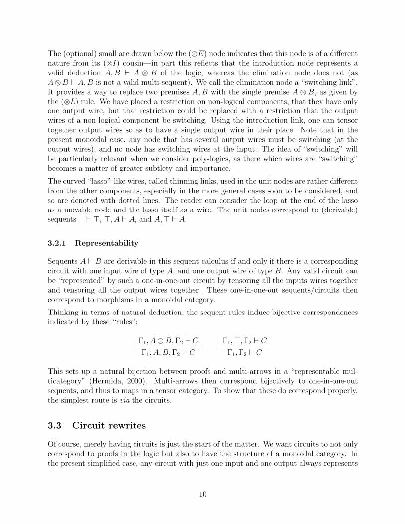
The (optional) small arc drawn below the (⊗E) node indicates that this node is of a differentnature from its (⊗I) cousin—in part this reflects that the introduction node represents avalid deduction A,B ` A ⊗ B of the logic, whereas the elimination node does not (asA⊗B ` A,B is not a valid multi-sequent). We call the elimination node a “switching link”.It provides a way to replace two premises A,B with the single premise A ⊗ B, as given bythe (⊗L) rule. We have placed a restriction on non-logical components, that they have onlyone output wire, but that restriction could be replaced with a restriction that the outputwires of a non-logical component be switching. Using the introduction link, one can tensortogether output wires so as to have a single output wire in their place. Note that in thepresent monoidal case, any node that has several output wires must be switching (at theoutput wires), and no node has switching wires at the input. The idea of “switching” willbe particularly relevant when we consider poly-logics, as there which wires are “switching”becomes a matter of greater subtlety and importance.

The curved “lasso”-like wires, called thinning links, used in the unit nodes are rather differentfrom the other components, especially in the more general cases soon to be considered, andso are denoted with dotted lines. The reader can consider the loop at the end of the lassoas a movable node and the lasso itself as a wire. The unit nodes correspond to (derivable)sequents ` >, >, A ` A, and A,> ` A.

3.2.1 Representability

Sequents A ` B are derivable in this sequent calculus if and only if there is a correspondingcircuit with one input wire of type A, and one output wire of type B. Any valid circuit canbe “represented” by such a one-in-one-out circuit by tensoring all the inputs wires togetherand tensoring all the output wires together. These one-in-one-out sequents/circuits thencorrespond to morphisms in a monoidal category.

Thinking in terms of natural deduction, the sequent rules induce bijective correspondencesindicated by these “rules”:

Γ1, A⊗B,Γ2 ` CΓ1, A,B,Γ2 ` C

Γ1,>,Γ2 ` CΓ1,Γ2 ` C

This sets up a natural bijection between proofs and multi-arrows in a “representable mul-ticategory” (Hermida, 2000). Multi-arrows then correspond bijectively to one-in-one-outsequents, and thus to maps in a tensor category. To show that these do correspond properly,the simplest route is via the circuits.

3.3 Circuit rewrites

Of course, merely having circuits is just the start of the matter. We want circuits to not onlycorrespond to proofs in the logic but also to have the structure of a monoidal category. Inthe present simplified case, any circuit with just one input and one output always represents

10

a morphism in a monoidal category. In general, we should expect there to be a more com-plicated “correctness” condition on circuits which corresponds to how proofs in the logic (ormaps in the categorical doctrine) are constructed. Shortly we shall meet such a correctnesscondition for poly-logics.

A question, arising not only from categorical considerations, but also from logic (Prawitz,1971), is: when are two morphisms or proofs equivalent? This is in some sense the fundamen-tal question for the logics we are discussing. It turns out that circuits are a very convenienttool for resolving this question. We shall now focus on this question.

There is an equivalence relation on circuits, generated by the following rewrites which wepresent as a reduction–expansion system modulo equalities.

Reductions:

j⊗j⊗ =⇒

A B

A B

A⊗B

A B

j>j> =⇒

�� ��

A A

(There is a mirror image rewrite for the unit, with the unit edge and nodes on the other sideof the A edge.)

Expansions:

j⊗

j⊗=⇒

A⊗B A⊗B

A B

A⊗B

j>j>> =⇒ �� ��(Again, there is a mirror image rewrite for the unit, with the thinning edge on the other sideof the unit edge and node.)

In addition to these rewrites, there are also a number of equivalences, see Figure 1, whichmust be imposed to account for the unit isomorphisms. These basic rewiring moves (Figure1) may be summarized by a result, originally proved by Todd Trimble in his PhD dissertation(and later published in (Blute, Cockett, Seely and Trimble, 1996)), which says that a thinninglink may be moved to any position in its “empire”, which essentially means from its initialposition to any wire which is connected to that position whatever the switch settings, wherethe thinning link itself is not used for that connection (details in (Blute, Cockett, Seely andTrimble, 1996)). The basic moves of Figure 1 give more “atomic” moves which generate thelarger “empire” moves. An example may be seen in Figure 5, where, for instance, the firststep moves a thinning wire on the far left up over the top of the circuit and down to the

11

right-hand side of the circuit. The next rewiring step then moves a thinning link top rightdown along the wires to a position bottom right (that move is possible, for each setting ofthe switches of the bottom two ⊕ links, because of the thinning wires which allow two pathsaround each ⊕ link). And so on . . .

At the basic monoidal level, these equivalences actually allow the unit lasso to be movedonto any wire—provided a circuit is produced (for example, there should be no cycles). Forthis reason, when dealing with this level of logic the thinning links will often be omitted.However, we shall shortly see why thinning links cannot be omitted in the setting with morestructure we shall consider. With that setting in mind, we have also included some diagramswith many outputs, which cannot occur in the monoidal setting. The reader should imaginea single output in those cases for now.

3.3.1 Normal Forms

Given the system of reductions and expansions, modulo equations, as described above, wecan show that the reduction and expansion rewrites terminate, that there is a Church-Rosser theorem, modulo equations, and so there is a notion of expanded normal form, againmodulo equations, for proof circuits. Essentially, the shape of a normal form involves tensorelimination steps (at the top), with some rearrangement of wires (in the middle), endingwith tensor introductions (at the bottom).

In the present case, all this is not too difficult to see. First notice that the reductionsalways remove material and so must certainly terminate. In contrast, the expansions alwaysintroduce material as the idea is that they “express” the type of the wire they expand. Onecan imagine repeatedly expanding a wire along its length. This means that the expansionsdo not terminate in the usual sense. However, in an expansion/reduction system, expansionswhich can be immediately removed by reduction (we call these reducible expansions) haveno net effect on the system. Thus, an expansion/reduction system works by reducing termsto reduced form and using irreducible expansions to move between reduced forms (this is asort of annealing process). This means one only applies expansion rules to reduced termsand, having applied the expansion, one immediately reduces the result. An expanded normalform is a reduced circuit for which all expansions are reducible.

Returning to the case of expanding a wire twice along its length, it is easy to see that thesecond expansion will immediately trigger a reduction back to the single expansion. Thus,a wire can only be expanded at most once on its length. A wire of composite type whenexpanded produces wires having strictly smaller types which can in turn be expanded in anested fashion. However, this sort of expansion nesting must terminate as the types of theproduced wires become strictly smaller. This shows that this expansion reduction systemterminates.

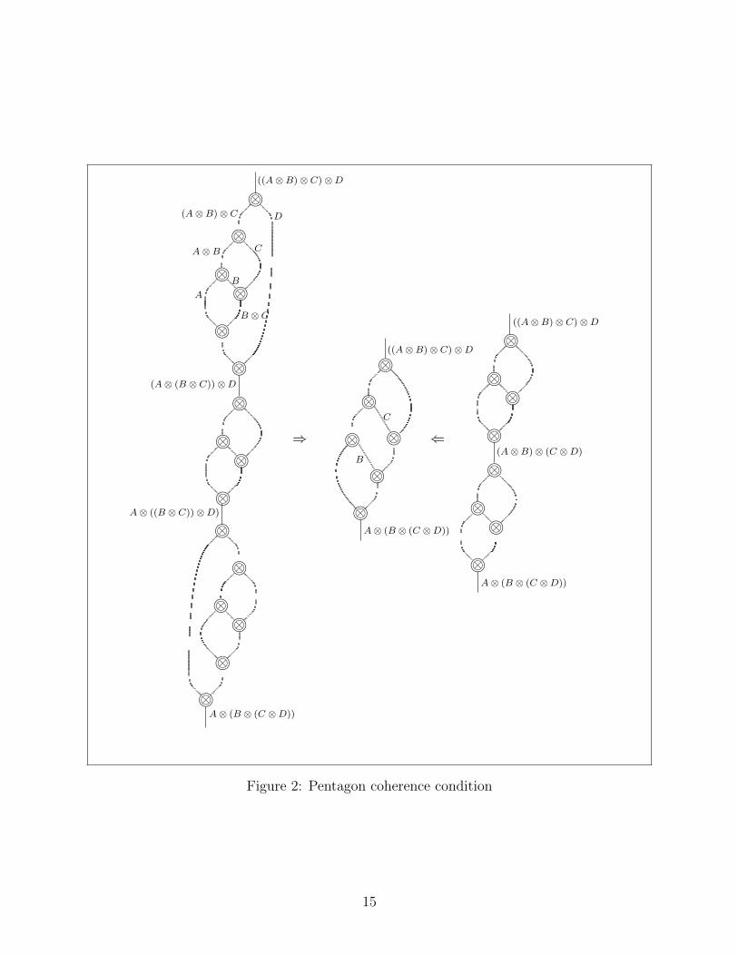
Two examples of rewriting are shown in Figure 2 and Figure 3. The former shows Mac Lane’spentagon coherence condition a�; a� = a� ⊗ 1; a�; 1 ⊗ a�: the left-hand side and the right-hand side of the equation are shown on the far left and far right. In the middle, the commonreduction shows they are equal. In this example, repeated use of the tensor reduction rule isall that is needed. To illustrate the need for the unit equivalence and the lassos, in Figure 3

12

j⊗

A B

A⊗B

j>�� ��>

= j⊗

A B

A⊗B

j>>�� �� j⊗A B

A⊗B

j>> j⊗A B

A⊗B

j>>=�� �� �� ��

j⊗A B

j>A⊗B>

j⊗A B

j>A⊗B>

=∗�� �� �� ��

j>>

A

�� ���� ��j>>

A

�� ��=

j>>

A

�� ��=j>>

j>>

j>>

�� ���� ��z1 z2 z1 z2 z1 z2

j>>

=

�� ��à A

f

∆ B

j>>Γ A

f

∆ B

�� ��

j>>

=f

A ∆ B

>>

f

A ∆ B

�� �� �� ��

j

j>>

f

j>>

f=

�� �� �� ��Γ1 A B Γ2

∆

>Γ1 A B Γ2

∆

j>=�� ��

A A

�� ��j>

> >

j>>

=

Γ

A B

f

∆1 ∆2

�� ��j>>Γ

A B

f

∆1 ∆2

�� ��

Figure 1: Unit rewirings

13

we show how the unit coherence condition (a�; 1⊗uL� = uR�⊗1) can be proven using circuits.

3.4 Summary so far

The proofs of a multi-logic may be presented as multi-arrows in a multicategory. These,in turn can be represented using circuit diagrams. In Section 5 we will provide a moreformal treatment of circuits. Representable multicategories are monoidal categories andthese correspond to ⊗-multi-logics. ⊗-multi-logics have a cut elimination theorem. Viewedas a rewriting system on circuits this becomes an expansion/reduction rewriting systemwhich allows one to decide equality of proofs. Finally, the equivalence classes of circuits(or of derivations) are morphisms of a category of circuits, and this is the free (symmetric)monoidal category (over a generating multi-graph of components).

We have already seen that circuits form a (symmetric) monoidal category where the objectsare formulas and morphisms are equivalence classes of circuits. That it is the free such is theforce of Mac Lane’s coherence theorem; a proof of these claims (in the linearly distributivecontext) may be found in (Blute, Cockett, Seely and Trimble, 1996). This may be summa-rized by the following conceptual diagram (which actually represents 2-equivalences betweenappropriate chosen 2-categories).

⊗-Multi-Logics66

vv

hh

((

⊗−Circuitsoo // Monoidal

Categories

4 Tensor and Par: basic components of linear logic

Imagine setting up a poly-logic: its sequents permit many (or no) premises on the left ofthe turnstile and many (or no) conclusions on the right of the turnstile. For the momentassume no commutativity: this means the cut rule has to take several forms which gives thefollowing presentation as a sequent calculus.

A ` A id

Γ ` A Γ1, A,Γ2 ` ∆

Γ1,Γ,Γ2 ` ∆cut1

Γ ` ∆1, A,∆2 A ` ∆

Γ ` ∆1,∆,∆2cut2

Γ1 ` ∆1, A A,Γ2 ` ∆2

Γ1,Γ2 ` ∆1,∆2cut3

Γ1 ` A,∆1 Γ2, A ` ∆2

Γ2,Γ1 ` ∆2,∆1cut4

One might have expected the identity axiom A ` A to have had a more general form asΓ ` Γ. However, that would correspond to what is known as the “mix” rule, and wouldgives the logic quite a distinct and different flavour. Among other things, the mix rule wouldallow a circuit to have several disconnected components; without mix, circuits have to beconnected. The circuits corresponding to the four cut rules are drawn below. Note that for

14

j

j

j

j

j

j

j

j

j

j

j

j

j

j

j

j

j j

j

j

j

j

jj

j

j

j

j

j

j

⊗

⊗

⊗

⊗

⊗

⊗

⊗

⊗

⊗

⊗

⊗

⊗

⊗

⊗

⊗

⊗

⊗ ⊗

⊗

⊗

⊗

⊗

⊗⊗

⊗

⊗

⊗

⊗

⊗

⊗⇒ ⇐

((A⊗B)⊗ C)⊗D

((A⊗B)⊗ C)⊗D

((A⊗B)⊗ C)⊗D

(A⊗B)⊗ C

A⊗B C

D

A

B

B ⊗ C

(A⊗ (B ⊗ C))⊗D

A⊗ ((B ⊗ C))⊗D)

A⊗ (B ⊗ (C ⊗D))

A⊗ (B ⊗ (C ⊗D))

A⊗ (B ⊗ (C ⊗D))

(A⊗B)⊗ (C ⊗D)

C

B

Figure 2: Pentagon coherence condition

15

j

j

j

j

jj

j

jj

j

jj⊗

⊗

⊗

⊗

⊗

⊗

⊗

⊗

⊗

⊗⇒

>

>

�� ���� ��

(A⊗>)⊗B

(A⊗>)⊗B

A⊗>B

>

A

A⊗ (>⊗B)

A

A

>⊗B

>⊗B

B

B

A⊗B

A⊗B

Figure 3: Unit coherence condition

simplicity, we have represented lists of formulas, such as Γ, as well as single formulas, suchas A, by single wires. In each case, the only wires that must correspond to single formulasare those that join the two boxes being cut.

The reader should notice that any circuit inductively built from these rules, that is a poly-circuit, not only must be connected but also cannot have any cycles (i.e. must be acyclic).This, in fact, is precisely the correctness criterion for poly-circuits.

This circuit calculus is the basis for the categorical structure of a polycategory, as discussedfor example in (Cockett and Seely, 1997b; Cockett et al., 2003). In fact, circuits over anarbitrary poly-graph, with their natural notion of equivalence and satisfying the correctnesscriterion, form the free polycategory over that poly-graph.

16

4.1 ⊗⊕-poly-logic

To capture the appropriate categorical notion, we must add appropriate tensor structures sothat the “commas” of poly-logic. on both sides of the poly-sequents, are represented. Thecommas on the left of the turnstile are interpreted differently from those on the right. Thusthere are two connectives: ⊗ (“tensor”) for commas on the left and ⊕ (“par”) for commas onthe right. The behaviour of these connectives is determined by requiring that polycategorybe representable in the sense that there are the following bijective correspondences betweenpoly-maps:

Γ1,Γ2 ` ∆

Γ1,>,Γ2 ` ∆

Γ ` ∆1,∆2

Γ ` ∆1,⊥,∆2

Γ1, X, Y,Γ2 ` ∆

Γ1, X ⊗ Y,Γ2 ` ∆

Γ ` ∆1, X, Y,∆2

Γ ` ∆1, X ⊕ Y,∆2

Translating this into a sequent calculus presentation gives the sequent calculus presentationof ⊗⊕-poly-logic. This consists of the cut rules of poly-logic, as above, together with thefollowing logical rules governing these new connectives:

Γ1,Γ2 ` ∆

Γ1,>,Γ2 ` ∆(>L) ` > (>R)

⊥ ` (⊥L)Γ ` ∆1,∆2

Γ ` ∆1,⊥,∆2(⊥R)

Γ1, X, Y,Γ2 ` ∆

Γ1, X ⊗ Y,Γ2 ` ∆(⊗L)

Γ1 ` ∆1, X Γ2 ` Y,∆2

Γ1,Γ2 ` ∆1, X ⊗ Y,∆2(⊗R)

Γ1, X ` ∆1 Y,Γ2 ` ∆2

Γ1, X ⊕ Y,Γ2 ` ∆1,∆2(⊕L)

Γ ` ∆1, X, Y,∆2

Γ ` ∆1, X ⊕ Y,∆2(⊕R)

The circuits that correspond to these rules are induced by the following basic nodes: thefamiliar tensor and tensor unit nodes from the tensor circuits, and dual nodes for the parand par unit ⊥.

(⊕I) j⊕A B

A⊕B

(⊕E)j⊕A⊕B

A B

(⊥I)L j⊥⊥

�� ��(⊥I)R j⊥

⊥

�� ��(⊥E)j⊥⊥

Using these components any proof of ⊗⊕-poly-logic may be represented by a circuit. How-ever, not every circuit made of these components represents a proof! Thus, to guaranteethat a circuit does represent a proof, there is an additional correctness criterion which mustbe satisfied. One way to express this correctness criterion, due to Girard, is by a “switchingcondition”: a circuit satisfies this condition if, whichever way one sets the “switch” in eachswitching link, the circuit remains connected and acyclic. To set the switch in a switching link

17

one disconnects one of the two wires between which the “switch” links. A circuit satisfyingthis correctness criterion (and thus represents a proof in ⊗⊕-poly-logic) is a ⊗⊕-circuit.

Notice that using this criterion one can demonstrate that a circuit does not satisfy thecorrectness criterion by a non-deterministic polynomial time (NP) algorithm. This algorithmworks by guessing a configuration of the switches and proving the circuit with that setof disconnections is either cyclic or disconnected. Providing a configuration of switchesto witness the incorrectness of a circuit is a very effective way of showing the invalidityof a circuit. So, the problem of determining correctness is a co-NP problem. To showthat a circuit satisfies the correctness criterion using this approach one must potentiallytry all possible switching configurations . . . and there are exponentially many of these.Algorithmically this would be somewhat disastrous!

Fortunately, Danos and Regnier (1989) describes a linear time algorithm for the correctnesscriterion which is based on more directly checking that a circuit represents a proof. Thiscorrectness criterion can easily be adapted for ⊗⊕-circuits and this is described in (Blute,Cockett, Seely and Trimble, 1996).

4.2 Why are thinning links necessary?

A curiosity is the apparent lack of symmetry between unit introduction and eliminationlinks. Logically they correspond to the (bijective) correspondences we saw above. We mighthave expected the > elimination link (>E) and the ⊥ introduction link (⊥I) to be withouta lasso. But this simply does not work! As this is a rather crucial aspect of our circuitcalculus, some discussion of this is in order.

We shall want circuit identities corresponding to the equivalence of the following proof (whichuses a cut on the left >) and the identity axiom:

> ` >` > >,> ` >

> ` >

(and dually for ⊥). If we had let the (>E) link be without lasso, as suggested above, thisidentity would become:

j>j> >=

This will not do, however—the lack of a thinning link here is fatal to the coherence questionswhich concern us. To see why, consider the following simple example which compares the

18

identity with the par twist map applied to the tensor unit “par”ed with itself:

j⊕

j⊕>⊕>

>⊕>

> > and

j⊕

j⊕>⊕>

>⊕>

> >

Given the above identity without thinning links these would both be equivalent to the samenet as expanding the wires of type > would lose the twist because the circuit becomesdisconnected.

j⊕

j⊕>⊕>

>⊕>

j> j>j> j>

The twist and the identity on > ⊕ > are not equivalent as morphisms.7 The point is thatwith thinning links we can at least distinguish these maps as nets, as we see below:

j⊕

j⊕>⊕>

>⊕>

j> >

j> jj>

�� �� �� ��and

j⊕

j⊕>⊕>

>⊕>

j> j>

j> j>

�� �� �� ��

so there is hope that we can arrange for them to be inequivalent (and indeed they are).Note, however, the different behaviour of the units: if we replace > with ⊥, then these netsdo correspond to equivalent derivations, since ⊥⊕⊥ is isomorphic to ⊥ and the identity is

7A remark for “experts”: an example of a linearly distributive category where this is the case isChu(Set, 2). This is more easily seen considering the dual ⊥ ⊗ ⊥. The unit ⊥ is the tuple 〈2, 1〉 (withthe obvious map 2× 1 −→ 2), and ⊥⊗⊥ = 〈2× 2, ∅〉 (with the empty map). It’s clear that the twist and theidentity are not equal.

19

the same as the twist on ⊥. Thus, these two nets when we expand the ⊥ identity wires inthe same manner must be equivalent.

j⊕

j⊕⊥⊕⊥

⊥⊕⊥

⊥ ⊥ and

j⊕

j⊕⊥⊕⊥

⊥⊕⊥

⊥ ⊥

To make these circuits equivalent it is clear that we must be able to rewire the thinninglinks in some manner, but equally not all rewirings can be permissible, so as to keep thedistinctions seen with the two maps > ⊕ > −→ > ⊕ > above. It is not too surprising thatrewirings will be required. Thinning links merely indicate a point at which a unit (or counit)has been introduced by thinning and there is considerable inessential choice going on here.For example, consider the three sequent calculus derivations of the sequent A,>, B −→ A⊗Bobtained by thinning in each of the possible places (these clearly should be equivalent):

A −→ A B −→ B A −→ A B −→ BA,B −→ A⊗B = A,> −→ A B −→ B = A −→ A >, B −→ BA,>, B −→ A⊗B A,>, B −→ A⊗B A,>, B −→ A⊗B

As circuits, these are just the (⊗I) node with a (>E) link attached to the three possible links.It turns out that the allowable rewirings are essentially those from Figure 1, their obvious“duals” involving ⊥ and ⊕, and a few involving interactions between these two structures(Blute, Cockett, Seely and Trimble, 1996).

4.3 Linearly distributive categories

To introduce linearly distributive categories, consider the following conceptual diagram, re-calling the connection between tensor circuit diagrams, multicategories, and monoidal cate-gories. This states the analogous connection between the various structures for two tensorsshould also hold. The intention behind the definition of a linearly distributive category is,thus, that it should be viewed as the (one-in-one-out) maps of a “representable polycate-gory”.

⊗⊕-Poly-Logics77

ww

gg

''

⊗⊕−Circuitsoo //

LinearlyDistributiveCategories

A linearly distributive category has two tensors: the “tensor” (⊗, a�, uL�, u

R�), and the “par”

(⊕, a�, uL�, u

R�) both satisfying the usual coherences of a tensor. The interaction of these

20

tensors is mediated (in the non-symmetric case) by two natural linear distribution maps:

δL:A⊗ (B ⊕ C) −→ (A⊗B)⊕ C δR: (B ⊕ C)⊗ A −→ B ⊕ (C ⊗ A)

These must satisfy a number of coherences which, categorically, may be seen as (linear)strength coherences. Before discussing these, however, it is worth understanding the mannerin which the linear distributions arise from the interaction of having representation for thecommas and the behaviour of the cut. The following derivation of δL demonstrates thisinteraction:

B ⊕ C ` B ⊕ C id

B ⊕ C ` B,C ⊕R A⊗B ` A⊗B id

A,B ` A⊗B ⊗L

A,B ⊕ C ` A⊗B,C Cut

A⊗ (B ⊕ C) ` (A⊗B)⊕ C ⊗L,⊕R

The definition of a linearly distributive category is subject to a number of symmetries thesearise from reversing the tensor (A ⊗ B 7→ B ⊗ A), reversing the par (A ⊕ B 7→ B ⊕ A)and reversing the arrows themselves while simultaneously swapping tensor and par (thusδL:A⊗ (B⊕C) −→ (A⊗B)⊕C becomes δR: (A⊕B)⊗C −→ A⊕ (B⊗C)). We present threecoherence diagrams which are complete in the sense that together with these symmetriesthey can generate all the coherences for (non-symmetric) linearly distributive categories:

>⊗ (A⊕B)uL�

&&δL

��(>⊗A)⊕B

uL�⊕B// A⊕B

(A⊗B)⊗ (C ⊕D)

δL

��

a� // A⊗ (B ⊗ (C ⊕D))

A⊗δL��

A⊗ ((B ⊗ C)⊕D)

δL

��((A⊗B)⊗ C)⊕D

a�⊕D// (A⊗ (B ⊗ C))⊕D

(A⊕B)⊗ (C ⊕D)

δL

tt

δR

**((A⊕B)⊗ C)⊕D

δR⊕D��

A⊕ (B ⊗ (C ⊕D))

A⊕δL��

(A⊕ (B ⊗ C))⊕D a�// A⊕ ((B ⊗ C)⊕D)

4.3.1 Negation

A key ingredient in the original account of linear logic, which is missing in linearly distributivecategories, is negation. So just what do we need to obtain negation in a linearly distributivecategory? First, we need a function (on objects), which we shall denote A 7→ A⊥. In thenon-symmetric case we shall need two such object functions A 7→ A⊥ and A 7→ ⊥A. Forsimplicity, we shall outline the symmetric case here, where ⊥A = A⊥. Also we need two

21

parametrized families of maps8:

A⊗ A⊥ γA−−→ ⊥ > τA−−→ A⊥ ⊕ A

which satisfy the following coherence conditions

A⊗> A⊗τA//

uR�

��

A⊗ (A⊥ ⊕A)

δL

��(A⊗A⊥)⊕A

γA⊕A��

A ⊥⊕AuL�

oo

>⊗A⊥ τA⊗A⊥//

uL�

��

(A⊥ ⊕A)⊗A⊥

δR

��A⊥ ⊕ (A⊗A⊥)

A⊥⊕γA��

A⊥ A⊥ ⊕⊥uR�

oo

As circuits, this is as follows. The links are represented as “bends”:

(γ) j¬A A⊥

(τ)

j¬A⊥ A

And the equivalences (rewrites) are these:

(¬ Reduction) j¬A

j¬A

A⊥ =⇒ A

(¬ Expansion) j¬A⊥

j¬A⊥

A=⇒A⊥

Of course, the hope is that the function A 7→ A⊥ is a contravariant functor, and the families of mapsare dinatural transformations. This is indeed the case. In fact, the category of ⊗⊕-circuits withnegation (in this sense) generated from a poly-graph is the free ∗-autonomous category generated bysaid poly-graph. The 2-category of linearly distributive categories with negation and linear functors(which we shall discuss shortly) is equivalent to the category of ∗-autonomous categories withmonoidal functors. Moreover, there is a conservative extension result, stating that the extension ofthe tensor-par fragment of linear logic to full multiplicative linear logic (which includes negation) isconservative. More precisely, the functor from the category of linearly distributive categories to thecategory of ∗-autonomous categories extends to an adjunction (the right adjoint being the forgetful

8We do not assume any naturality for these maps. In fact, they turn out to be dinatural transformations.

22

functor), whose unit is full and faithful, and whose counit is an equivalence (Blute, Cockett, Seelyand Trimble, 1996).

One consequence of this is that we now have a good circuit calculus for ∗-autonomous categories—the categorical doctrine corresponding to multiplicative fragment of linear logic—and this allowsus to give a decision procedure for equality of maps in these categories. Bear in mind that thisdecision procedure necessarily involves a search as this is a pspace complete problem (Heijltjesand Houston, 2014) and so is not very efficient! As an example of this at work, here is a classicproblem (not completely solved until (Blute, Cockett, Seely and Trimble, 1996)), usually called thetriple-dual diagram:

((A−◦ I)−◦ I)−◦ I1

ttkA−◦1

))((A−◦ I)−◦ I)−◦ I oo

kA−◦1(A−◦ I)

(using kA : A −→ ((A−◦ I)−◦ I), the exponential transpose of evaluation.)

In ∗-autonomous categories, (or monoidal closed categories), this diagram generally does not com-mute. This is easy to see if I is not a unit. If I is a unit, then the diagram does commute if I = ⊥,generally does not commute if I = >, but does commute if A = I = >.

We note that such instances of this diagram in fact can be done in the linearly distributive context,if we define the internal hom as a derived operation: A−◦B = A⊥⊕B, replace I with a unit and I⊥

with the other unit, and replace the negation links with appropriate derived rules corresponding tothe (iso)morphisms >⊗⊥ −→ ⊥ and > −→ ⊥⊕>. Then we translate the composite kA−◦1; kA −◦ 1above into a proof net: the left side of Figure 4 is a step on the way to its expanded normal form(we write B for A⊥ to prepare for the version of the net that may be constructed in the linearlydistributive context). The right side is a similar step in calculating the expanded normal form ofthe identity circuit.

In the circuits of Figure 4, if I were not a unit, these would be the expanded normal forms,and clearly these nets are not the same. An old idea due to Lambek (1969) may be seen here:the “generality” of the first net is clearly a derivation of the sequent ((B ⊕ C) ⊗ C⊥) ⊕ D −→((B⊕D)⊗E⊥)⊕E, whereas the generality of the second is ((B⊕C)⊗D)⊕E −→ ((B⊕C)⊗D)⊕E.This is no surprise; it is exactly what one would expect if I was not a unit. Next consider the caseif I is a unit.

If I = >, say, then the nodes at I and I⊥ have to be expanded, since in expanded normal form,each occurrence of a unit (recall >⊥ = ⊥) must either come from or go to a null node. This ineffect transforms several of the edges in the graphs above into thinning links. We leave it as anexercise to show that in this case no rewiring is possible, and hence the diagram does not commute.And similarly that the rewiring may be done if I = ⊥, so that diagram does commute.

But now consider the case where A = I = > (where the diagram commutes). We must show howto rewire the net corresponding to the compound morphism to give the identity. This is shown inFigure 5: the point here is that with A = > we have an extra unit and thinning link (correspondingto the wire/thinning link for ⊥ replacing B at the left), which has a possible rewiring. Although itis not immediately obvious why this thinning link should be rewired, doing so makes other rewiringspossible, and once the required rewirings are done, the initial rewiring is reversed to finish with theexpanded normal form of the identity map.

23

j⊗j⊕

j⊗

j⊕

j⊕j⊕j¬

j¬

((B ⊕ I)⊗ I⊥)⊕ I

I

I

I⊥

B

I⊥

I

((B ⊕ I)⊗ I⊥)⊕ I

j⊗j⊕

j⊗

j⊕

j⊕j⊕

((B ⊕ I)⊗ I⊥)⊕ I

II I⊥B

((B ⊕ I)⊗ I⊥)⊕ I

Figure 4: Two sides of the triple-dual triangle

5 Circuits

While the circuits diagrams provide a convenient representation of morphisms or proofs, they havea formal underpinning which is also of interest. Although it is tempting to conflate the two notions,a circuit diagram is, in fact, a diagrammatic representation of something more fundamental, whichwe call a circuit. Circuits provide a term logic for monoidal settings. Such term logics have adistinguished pedigree, going back to Einstein’s summation notation for vector calculations9, andincluding diagram notations by Feynman and by Penrose, for example. Their notations were moreconcretely attached to the specifics of the vector space contexts for which they were intended. Ourcircuits—which are derived not only from Girard’s proof nets but also from the work of Joyal andStreet (1991)—are intended to be more general. Vector space manipulations are a canonical exampleof tensor category manipulations, so that there is a direct ancestry is not a surprise. However, unlikeour predecessors, including Joyal and Street, we explicitly intended our notation to be a term logic,and in particular we applied it to solve the coherence problems associated with linearly distributivecategories. Despite this, the term logic was initially invented to facilitate calculations in monoidalcategories, and so we shall return to this more straightforward application in the present essay. Toextend these ideas to the full linearly distributive case involves adding the structures which we havedescribed above using—the more user friendly but equivalent representation—circuit diagrams.

We start by making precise the notion of a typed circuit. To build a typed circuit one needs a setof types, T , and a set of components, C. Each component f ∈ C has a signature sig(f) = (α, β),a pair of lists of types, where α is the types of the input ports and β the types of the outputports.

9We thank Gordon Plotkin for bringing this to our attention.

24

h⊗h⊕

h⊗

h⊕

h⊕h⊕

h>h⊥

h⊥

h>h⊥h⊥

h>

h>

������ ���� ��

����

=⇒

((⊥⊕>)⊗⊥)⊕>

((⊥⊕>)⊗⊥)⊕>

h⊗h⊕

h⊗

h⊕

h⊕h⊕

h>h⊥

h⊥

h>h⊥h⊥

h>

h>

������ ��

����

�� �� =⇒

h⊗h⊕

h⊗

h⊕

h⊕h⊕

h>h⊥

h⊥

h>h⊥h⊥

h>

h>

����

����

�� ���� ��

=⇒

h⊗h⊕

h⊗

h⊕

h⊕h⊕

h>h⊥

h⊥

h>h⊥h⊥

h>

h>

����

�� ���� ��

����

=⇒

h⊗h⊕

h⊗

h⊕

h⊕h⊕

h>h⊥

h⊥

h>h⊥h⊥

h>

h>�� ���� ��

������ ��

=⇒

h⊗h⊕

h⊗

h⊕

h⊕h⊕

h>h⊥

h⊥

h>h⊥h⊥

h>

h>�� ��

������ ���� ��

Figure 5: Rewiring the triple-dual

25

To obtain a primitive circuit expression one attaches to a component two lists of variables.Thus, if sig(h) = ([A,B], [C,D]), then we may write

hx1,x2y1,y2

the variables in the superscripted list are the input variables: each variable must have the correcttype for its corresponding port so x1:A (viz x1 is of type A) and x2:B. The subscripted variablelist contains the output variables and they must have types corresponding to the output ports, soy1:C, and y2:D. The variable names in each list must be distinct. The resulting (primitive) circuitexpression has a list of input variables [x1, x2] and a list of output variables [y1, y2].

In the more familiar term logic associated with algebraic theories one does not have output variables.To emphasize that they are something peculiar to this “monoidal” term logic, Lambek referred tothem as covariables. While we shall not adopt this terminology here, we shall discover that theterm does convey their intent.

h

A B

C D

A primitive circuit presented as a circuit diagram is just a box with a number of(typed) input and output ports. The input wires in this diagram represent the list oftyped input variables and the output wires represent the list of typed output variables.

g

f

X1 X2 X3 X4

Y1 Y2 Y3 Y4 Y5

One “plugs” (primitive) circuit expressions together to form new circuit expres-sions by juxtaposition, just as one attaches two circuit diagrams together:

fx2,x3y1,z1,y5,z2 ; gx1,z2,x4,z1y2,y3,y4

The output variables of the first component which are common to the input vari-ables of the second component become bound in this juxtaposition and indicatehow the components are connected. An output variable when it is bound inthis juxtaposition is bound to a unique input variable, or in Lambek’s termi-nology, covariables bind to unique variables. To perform a legal juxtapositionthe unbound input variables must be distinct and, similarly, the unbound out-put variables must be distinct. A variable clash occurs when this requirement is

violated. One can always rename variables to avoid variable clashes.

When one avoids variable clashes, the juxtaposition operation is associative. Furthermore, when ajuxtaposition does not cause any output variable to became bound to any input variables, one canexchange the order of the juxtaposition.

Notice that we have allowed the wires representing the bindings of z1 and z2 to “cross”, and indeedto access x1 and x4 as inputs also requires crossings. Allowing wires to cross in this mannercorresponds to having commutativity of the underlying logic. To obtain a nonsymmetric or planarjuxtaposition, we would have to properly treat the inputs and outputs as lists of variables instead ofviewing them as bags (or multi-sets). This would require that we alter the criteria for juxtaposition(the details are explicitly given in (Blute, Cockett, Seely and Trimble, 1996)).

A (non-planar) circuit expression C can be abstracted by indexing it by a non-repeating list ofinput and output variables. This is written⟨

C |x1,...,xny1,...,ym

⟩Furthermore one can indicate the types of the input and output wires by the notation:⟨

C |x1:T1,...,xn:Tny1:T ′1,...,ym:T ′m

⟩26

An abstraction must be closed in the sense that all the free input variables of C occur in theabstracting input variable list and all the free output variables of C occur in the abstracting outputlist. Furthermore, any variable in the abstracting input list which is not a free input of C mustoccur in the abstracting output list and, similarly, any variable in the abstracting output list whichis not a free output of C must occur in the abstracting input list.

In particular, we can use this technique of abstracting to isolate a wire (or many wires) as⟨∅ |x:T

x:T

⟩,

where ∅ is the empty circuit and the unit for juxtaposition. This is to be regarded as the “identitymap” on the type T . The ability to abstract (and the existence of an empty circuit) are importantwhen we consider how to form categories from circuits.

When a circuit expression is abstracted in this fashion all the wire names become bound. Externallyan abstraction presents only a list of typed input ports and a list of typed output ports. This permitsan abstracted circuit expression to be used as if it were a primitive component. An abstraction usedas a component is equivalent to the circuit obtained by removing the abstraction with a substitutionof wires outward with a renaming of the bound internal wires away from the external wires so asto avoid variable clashes. To see why the variables of the abstraction are used to substitute theexternal wires it suffices to consider the use of the “identity” abstraction mentioned above (orindeed any abstraction with “straight-through” wires):

〈〈∅ |xx〉yz |yz〉 =⇒ 〈∅ |xx〉

The operation of removing an abstraction we call abstraction dissipation; it is analogous toa β-reduction. The reverse operation is to coalesce an abstraction. These operations becomeparticularly important when we consider how one adds rules of surgery, as discussed below. In thenon-symmetric case, a planar abstraction must also preserve the order of the wires.

We may now define the notion of a (non-planar) circuit based on a set of components:

Definition 5.1 (Non-planar circuits)

(i) C–circuit expressions are generated by:

• The empty circuit, ∅, is a circuit expression,

• If c1 and c2 are circuit expressions which can be juxtapositioned (with no variable clash)then c1; c2 is a circuit expression,

• If f ∈ C is a component with sig(f) = (α, β) and V is a non-repeating wire list withtype α and W is a non-repeating wire list with type β then fVW is a circuit expression,

• If F is an abstracted circuit with signature sig(F ) = (α, β) and V is a non-repeatingwire list with type α and W is a non-repeating wire list with type β then F VW is a circuitexpression.

(ii) A circuit is an abstracted circuit expression.

One circuit expression (and by inference circuit) is equivalent to another precisely when one canobtain the second from the first by a series of the following operations:

• Juxtaposition reassociation (with possible bound variable renaming to avoid clashes),c1; (c2; c3) = (c1; c2); c3,

27

• Empty circuit elimination and introduction, c; ∅ = c = ∅; c,

• Exchanging non-interacting circuits, c1; c2 = c2; c1,

• Renaming of bound variables,

• Abstraction coalescing and dissipating.

The fact that circuit equivalence under these operations is decidable is immediately obvious whenone presents them graphically. Indeed, while it is nice to have a syntax for circuits it is very muchmore natural and intuitive to simply draw them!

The C–circuits, besides permitting these standard manipulations, can also admit arbitrary addi-tional identities. These take the form of equalities, c1 = c2, between (closed) abstracted circuitswith the same signature. To use such an identity in a circuit, it is necessary to be able to coalesceone of the sides, say c1 (up to α-conversion) within the circuit. Once this has been done one canreplace c1 with c2 and dissipate the abstraction. Diagrammatically this corresponds to a surgicaloperation of cutting out the left-hand side and replacing it with the right-hand side. Accordinglysuch additional identities are often referred to as rules of surgery. The circuit reductions andexpansions we saw earlier are examples of such rules of surgery.

5.0.2 ⊗-circuits: a term logic for monoidal categories

The basic components required to provide a circuit-based term logic for monoidal categories are asfollows:

(⊗I)A,BA⊗B ⊗–introduction

(⊗E)A⊗BA,B ⊗–elimination

(>I)> unit introduction

(>RE)A,>A unit right elimination (thinning)

(>LE)>,AA unit left elimination (thinning)

The rules of surgery providing the reduction system for ⊗-multi-logic are expressed as follows:

⟨(⊗I)x1,x2z ; (⊗E)zy1,y2 |

x1:A,x2:By1:A,y2:B

⟩⇒

⟨|x1:A,x2:Bx1:A,x2:B

⟩(1)⟨

(>I)z; (>LE)z,x1x2 |x1:Ax2:A

⟩⇒

⟨|x:Ax:A

⟩(2)⟨

(>I)z; (>RE)x1,zx2 |x1:Ax2:A

⟩⇒

⟨|x:Ax:A

⟩(3)

The rules of surgery providing the expansion rules for ⊗-multi-logic are next. Recall these shouldbe thought of as expressing the type of the wire:

28

⟨|z:A⊗Bz:A⊗B

⟩⇒

⟨(⊗E)zz1,z2 ; (⊗I)z1,z2z |z:A⊗Bz:A⊗B

⟩(4)⟨

|x:>x:>

⟩⇒

⟨(>I)z; (>LE)z,x1x2 |

x1:>x2:>

⟩(5)⟨

|x:>x:>

⟩⇒

⟨(>I)z; (>RE)x1,zx2 |

x1:>x2:>

⟩(6)

(7)

We shall leave as an exercise for the reader the translation of the unit rewirings into this termcalculus—graphically they were given in Figure 1. For example, the first one may be written thus:⟨

(>RE)x,zx ; (⊗I)x,yw |x:A,z:>,y:Bw:A⊗B

⟩=⟨

(>LE)z,yy ; (⊗I)x,yw |x:A,z:>,y:Bw:A⊗B

⟩As an illustration of the term calculus at work, consider the following example which is the coherencecondition for the tensor unit as shown in Figure 3. We shall write the variables x1, x2, . . . as simply1, 2, . . . , numbering the wires, top to bottom, left to right. In this way, the topmost link in the lefthand diagram is (⊗E)1

2,3 (wire 1 comes into the (⊗E) link, and wires 2, 3 leave it, 2 on the left, 3 onthe right, so that 1 refers to a wire of type (A⊗>)⊗B, 2 to a wire of type A⊗>, and 3 to a wireof type B). Here are the details of the rewriting showing the coalescing, surgery and dissipationsteps:⟨

(⊗E)12,3; (⊗E)2

4,5; (⊗I)5,36 ; (⊗I)4,6

7 ; (⊗E)78,9; (⊗E)9

10,11; (>LE)10,1111 ; (⊗I)8,11

12 |112

⟩=

⟨(⊗E)1

2,3; (⊗E)24,5; (⊗I)5,3

6 ;⟨

(⊗I)4,67 ; (⊗E)7

8,9 |4,68,9

⟩4,7

8,9; (⊗E)9

10,11; (>LE)10,1111 ; (⊗I)8,11

12 |112

⟩⇒

⟨(⊗E)1

2,3; (⊗E)24,5; (⊗I)5,3

6 ;⟨|4,64,6

⟩4,6

8,9; (⊗E)9

10,11; (>LE)10,1111 ; (⊗I)8,11

12 |112

⟩(⊗-reduction)

=⟨

(⊗E)12,3; (⊗E)2

4,5; (⊗I)5,36 ; (⊗E)6

10,11; (>LE)10,1111 ; (⊗I)4,11

12 |112

⟩=

⟨(⊗E)1

2,3; (⊗E)24,5;⟨| (⊗I)5,3

6 ; (⊗E)610,11 |

5,310,11

⟩5,3

10,11; (>LE)10,11

11 ; (⊗I)4,1112 |112

⟩⇒

⟨(⊗E)1

2,3; (⊗E)24,5;⟨|5,35,3

⟩5,3

10,11; (>LE)10,11

11 ; (⊗I)4,1112 |112

⟩(⊗-reduction)

=⟨

(⊗E)12,3; (⊗E)2

4,5; (>LE)5,311 ; (⊗I)4,11

12 |112

⟩=

⟨(⊗E)1

2,3; (⊗E)24,5

⟨(>LE)z,yy ; (⊗I)x,yw |x,z:>,yw

⟩4,5,3

12|112

⟩(coalescing)

=

⟨(⊗E)1

2,3; (⊗E)24,5

⟨(>RE)x,zx ; (⊗I)x,yw |x:A,z:>,y:B

w:A⊗B

⟩4,5,3

12|112

⟩(surgery: tensor unit axiom)

=⟨(⊗E)1

2,y; (⊗E)2x,z(>RE)x,zx ; (⊗I)x,yw |1w

⟩(dissipation)

=⟨

(⊗E)12,3; (⊗E)2

4,5(>RE)4,54 ; (⊗I)4,3

6 |16⟩

(renaming).

This amply illustrates why it is so attractive to work with the diagrammatic representation! How-ever, it is important to know that under the hood of circuit diagrams there is a fully formal (ifsomewhat verbose) notion of circuits which, for example, could be implemented on a computer.

29

6 Functor boxes

The use of circuit diagrams—and similar graphical tools using similar but different conventions—isvery widespread, and includes applications to systems developed for handling quantum computing(dagger categories) and for fixpoints and feedback (traced monoidal categories). They are evena useful device in understanding the categorical proof theory of classical logic. It is well-knownthat the usual Lambek-style approach collapses to posetal proof theory, so one cannot distinguishbetween proofs of the same sequents. However, interesting non-posetal proof theory for classicallogic may be obtained by a construction on top of the proof theoretic substrate provided by lin-early distributive categories or ∗-autonomous categories (Fuhrmann and Pym, 2007; Lamarche andStraßburger, 2005, 2006).

For the category theorist, one question is always paramount: what are the morphisms? In thepresent context, what would be the suitable functors between linearly distributive categories? Whatlogical structure would be suitable for handling interpretations from one poly-logic to another?And specifically, one is led to such questions as how would one represent modal operators (or otheroperators, for that matter) in poly logic? How would we adapt circuits to this purpose?

The answer we developed, in (Cockett and Seely, 1999), was a description of circuits for structuredfunctors, and indeed, is sufficient to account for a variety of logics, including a simple linear modallogic (Blute et al., 2002). The basic idea is similar to the proof boxes of Girard (1987) for theexponentials ! and ? , as described in (Blute, Cockett and Seely, 1996). But for more generalfunctors, a slightly different approach was needed, which we shall sketch here. Full details areavailable in (Cockett and Seely, 1999).

The first question to address is how to handle functors, indeed, “why do functors at all?” (i.e.“why boxes?”!). We shall see an example at the end of this section: modal logic. The first use ofboxes was by Girard (1987) for the exponentials ! and ? , which were called modalities from thebeginning. They were necessary to be able to interpret intuitionistic logic in linear logic, and infact were really the reason for his initial development of linear logic. More traditional modal logicwould also seem to require functors for @ and ♦ (necessity and possibility). But we must handlethese at the level of derivations (as well as formulas), so in effect we need to be able to “apply” themodalities to morphisms as well as to formulas. And the simplest way (or so it seems!) is to simplytake a subgraph corresponding to a derivation, and replace it with one corresponding to the imageof that derivation under the modality. And that is easily handled with the boxes we shall describebelow. Interestingly, this notion was independently discovered by Mellies (2006).

We start with an ordinary functor F : C −→ D. Given a morphism f :A −→ B in C, represented asa component with input wire of type A and output wire of type B, the corresponding morphismF (f):F (A) −→ F (B) in D is represented by simply “boxing” the component, as shown in Figure 6.

Note that the box bears a label with the name of the functor. These functor boxes have one inputand one output. If the component f is a poly-map, then it is necessary to tensor the inputs and parthe outputs to obtain a one-in-one out map before the functor box can be applied. We shall relaxthis condition soon in discussing monoidal and linear functors. The half oval through which thewire leaves the box is called the “principle port”. This is not really essential here, but we includeit for comparison with the structured boxes that will be described next: at that point its role willbecome clear. Notice also the typing changes the box imposes on a wire as it passes into or out ofa box.

There are two obvious rewrites to express functoriality: an “expansion” which takes an identity

30

f

�� �

F (A)

A

B

F (B)

F

Simple

functor boxf

�� �

F (B)

B

D

F (D)

F

F (C)

C

F (A)

AMonoidal

functor box

Figure 6: Simple and monoidal functor boxes

wire of type F (A) and replaces it with an identity wire of type A which is then “boxed”, and a“reduction” which “merges” two functor boxes one of which directly “feeds” into the next (box“eats” box).

Now we consider the situation where there is some structure on both categories and functor. Sup-pose first that the categories are monoidal categories, and the functor is also monoidal, meaningthat preservation of the tensor is lax. The functor F is monoidal if there are natural transformationsm� : F (A)⊗ F (B) −→ F (A⊗B) and m> : > −→ F (>) satisfying the equations

uL� = m>⊗1;m�;F (uL�) : >⊗ F (A) −→ F (A)

a�; 1⊗m�;m� = m�⊗1;m�;F (a�)

: (F (A)⊗ F (B))⊗ F (C) −→ F (A⊗ (B ⊗ C))

and in the symmetric case, the next equation as well:

m�;F (c�) = c�;m� : F (A)⊗ F (B) −→ F (B ⊗A)

We will soon also want the dual notion (for the dual par ⊕): a functor G is comonoidal if there arenatural transformations n� : G(A⊕B) −→ G(A)⊕G(B) and n⊥ : G(⊥) −→ ⊥ satisfying equationsdual to those above.

To capture the effect in circuits of requiring a functor to be monoidal, we modify the effect of the“functor box”, as shown in Figure 6.

m⊗� � �A⊗BF (A⊗B)

F

F (B)

B

F (A)

A

Note that for F monoidal, we may relax the supposition that the boxed subgraphis “one-in-one-out” to allow multi-arrows which have many input wires (but stilljust one output wire). One might expect that we would have to add componentsrepresenting the two natural transformations m�,m> that are necessary for F tobe monoidal. However, it is an easy exercise to show that these can be inducedby the formation rule for monoidal functor boxes: m> is the case where f is the(> I) node (no inputs and one output >), and m� is shown left.

There are reduction and expansion rewrites for these boxes (and one for handling “twists” permittedby symmetry). The necessary reduction rewrite is shown in Figure 7 (we refer to this saying onebox “eats” the other). And the “expansion” rule and the “twist” rule are shown in Figure 8

We have already indicated what the nets are for m�,m>. It is a fairly straightforward exercise toshow that the equations are consequences of the net rewrites given above, and that the rewrites

31

f

�� �

F (B)

B

Y

F

F (C)

C

F (A)

A

g

�� �Y

D

F (D)

F

F (Z)

Z

F (X)

X

F (Y ) =⇒

g

f

�F

� �

F (X)

F (A) F (B) F (C)

F (Z)

X

A B C

ZY

D

F (D)

Figure 7: Box-eats-box rule

�F� �=⇒

F (A) F (A)

A

�Ff

�Ff

=⇒

� � � �

Figure 8: Expansion and twist rules

32

j⊗j⊗

j⊗j⊗� �� �

j⊗j⊗

j⊗j⊗� �

=⇒

j⊗j⊗jjjjjj

⊗

⊗

⊗

⊗

⊗

⊗

� �� �

� �

j⊗j⊗jjjjjj

⊗

⊗

⊗

⊗

⊗

⊗� �

⇐= ⇐=

Figure 9: Functor boxes are monoidal—reassociation

correspond to commutative diagrams, if F is monoidal. (An exercise we leave for the reader(!)—but recall that the details may be found in (Cockett and Seely, 1999).) As an example, Figure 9shows that the equation dealing with “reassociation” is true for any F whose functor boxes satisfythe circuit rewrites we have given so far. So this circuit syntax is indeed sound and complete formonoidal functors. For comonoidal functors, we just use a dual syntax, with the correspondingrewrites. Note then that for comonoidal functors, the principle port will be at the top of the box(this is the role of the principle port, to distinguish monoidal functors from comonoidal ones).

6.1 Linear functors

To handle linear logic, it turns out that the suitable notion of functor is what we call a “linearfunctor”: this is really a pair of functors related by a shadow of duality. This duality becomesexplicit in the presence of negation (i.e. when the category is ∗-autonomous), for then the pair offunctors are de Morgan duals. This is discussed in more detail in (Cockett and Seely, 1999).

So, a linear functor F : C −→ D between linearly distributive categories C,D, consists of:

1. a pair of functors F�, F� : X −→ Y such that F� is monoidal with respect to ⊗, and F� iscomonoidal with respect to ⊕,

2. natural transformations (called “linear strengths”)

νR� : F�(A⊕B) −→ F�(A)⊕ F�(B)

νL� : F�(A⊕B) −→ F�(A)⊕ F�(B)

νR� : F�(A)⊗ F�(B) −→ F�(A⊗B)

νL� : F�(A)⊗ F�(B) −→ F�(A⊗B)

33

f

�� �

F�(B)

B

Y

F�(Y )

F

F�(C)

C

F�(A)

A

F�(Z)

Z

F�(X)

X

Linear

functor box

Figure 10: Linear functor box

satisfying coherence conditions corresponding to the requirements that the linear strengths areindeed strengths, and that the various transformations are compatible with each other. (These arelisted explicitly in (Cockett and Seely, 1999).) A representative sample is given here—the rest aregenerated by the obvious dualities.

νR� ;n⊥ ⊕ 1;uL� = F�(uL�)

F�(a�); νR� ; 1⊗ νR� = νR� ;n� ⊕ 1; a�

F�(a�); νR� ; 1⊗ νL� = νL� ; νR� ⊕ 1; a�

1⊗ νR� ; δLL ; νR� ⊕ 1 = m�;F�(δLL); νR�

1⊗ νL� ; δLL ;m� ⊕ 1 = m�;F�(δLL); νL�

In (Cockett and Seely, 1999) the definition of linear transformations, which are necessary to describethe 2-categorical structure of linear logic, is also given; but we shall not pursue that further here.

Now we extend the syntax of functor boxes to linear functors. In fact all that is necessary isto generalize the monoidal boxes to allow the boxed circuit to have arbitrarily many inputs andoutputs. So for the monoidal component F� of a linear functor F , the functor boxes will have theformation rule shown in Figure 10, and the comonoidal component will have the dual rule (justturn the page upside down). Please note the typing of this formation rule carefully: at the top ofthe box, the functor applied is the functor F� associated with the box, but at the bottom, onlythe wire that leaves through the principal port gets an F� attached to it, the other wires get thecomonoidal F� attached to them. (The dual situation applies for the F� boxes.) This is the role ofthe principal port in our notation (and is similar to the notation used in (Blute, Cockett and Seely,1996) for the “exponential” or “modal” operators ! and ? ). There may be only one principal port,though there may be arbitrarily many other (“auxiliary”) ports.

It is then quite easy to represent the νR� map as a boxed (⊕ E) node—the right output wire of thenode passes through the principal port. The three other linear strengths are given similarly: νL⊗ isthe (⊕ E) node boxed with a F� box, the left output wire passing through the principal port. Thetwo ν� maps are given by the (⊗ I) node boxed by the F� box, with either the right or the leftinput ports being the principal port, as appropriate.

Associated with these box formation rules are several rewrites. The expansion rewrite remains asbefore, but the reduction rewrite must be generalized to account for the more general f ; this is

34

done in the obvious fashion. Similarly, in the symmetric case we generalize the rewrites that movea “twist” outside a box. In fact, in the symmetric case it is convenient to regard the order ofinputs/outputs as irrelevant, so that these rewrites are in fact equalities of circuits. In addition,we must account for the interaction between F� and F� boxes, which gives a series of rewritesthat allow one box to “eat” another whenever a non-principal wire of one type of box becomes theprincipal wire of the dual type. We give an example of this in Table 1, along with the other rulesmentioned in this paragraph. The reader may generate the dual rules. Note that in this Tablewe have illustrated circuits with crossings of wires; in the nonsymmetric case, such crossings mustnot occur, so some wires must be absent from these rewrites. The rewrites dealing with pulling a“twist” out of a box are only relevant in the symmetric case of course. We have illustrated one,where the “twisted” wires are inputs; it is also possible that the “twisted” wires are outputs, andone may (or may not) be the wire through the principle port.

These rules are sound and complete; we must verify that any F = (F�, F�) which allows sucha calculus is indeed a linear functor, and conversely, that any linear functor allows such rewrites(Cockett and Seely, 1999). More interestingly, however, is what can be done with such functors(and their circuits). The key fact is that all the basic structure of linear logic (with the exceptionof negation) can be described in terms of linear functors: in a natural manner, tensor and partogether form a linear functor, as do Cartesian product and coproduct. And not surprisingly, so dothe exponentials ! and ? . If negation is added to the mix (so the category is ∗-autonomous, notmerely linearly distributive), then each pair consists of de Morgan duals, and in that context, thepair really just amounts to the monoidal functor in the pair (the comonoidal functor just being itsde Morgan dual).

There is a natural logic associated with a linear functor. A special case is illuminating. Consider alinear functor F : X −→ X. Write @ for F� and ♦ for F�. We shall not give a complete descriptionof the logic one obtains from this (Blute et al., 2002), but here are some highlights:

νL� : @ (A⊕B) −→ @A⊕♦Bm�: @A⊗ @B −→ @(A⊗B)

In a classical setting, these would be equivalent to

@(A⇒ B) −→ (@A⇒ @B)

@A ∧ @B −→ @(A ∧B)

the first being “normality” of the logic, and the second being one half (the linear half!) of thestandard isomorphism

@A ∧ @B ←→ @(A ∧B)

The following rule (and its dual cousins) holds in basic linear modal logic:

A1, A2, · · · , Am, B ` C1, C2, · · · , Cn@A1,@A2, · · · ,@Am,♦B ` ♦C1,♦C2, · · · ,♦Cn

This is a familiar rule in many modal situations, for example it occurs in the process calculus ofHennessy and Milner (1985).

References

Blute, R., Cockett, J.R.B. and Seely, R.A.G. (1996), ! and ?—storage as tensorial strength, Math-ematical Structures in Computer Science 6(04), 313–351.

35

�F�

f�F�

f

==

� � � ����

LLL ��TT

���

BB

��AABBB

��

�F�

� �=⇒

F�(A)

f

�� �

F�

g

�� �

F�

=⇒

g

f

�F�

� �

f

�� �

F�

g

F�

=⇒

g

f

�F�

� ��� �

Table 1: Some reduction and expansion rewrites for functor boxes

36

Blute, R., Cockett, J.R.B. and Seely, R.A.G. (2002), The logic of linear functors, MathematicalStructures in Computer Science 12(4), 513–539.

Blute, R., Cockett, J.R.B., Seely, R.A.G. and Trimble, T. H. (1996), Natural deduction and coher-ence for weakly distributive categories, Journal of Pure and Applied Algebra 113(3), 229–296.

Cockett, J.R.B., Koslowski, J. and Seely, R.A.G. (2000), Introduction to linear bicategories, Math-ematical Structures in Computer Science 10(02), 165–203.

Cockett, J.R.B., Koslowski, J. and Seely, R.A.G. (2003), Morphisms and modules for poly-bicategories, Theory and Applications of Categories 11(2), 15–74.

Cockett, J.R.B. and Seely, R.A.G. (1997a), Proof theory for full intuitionistic linear logic, bilinearlogic, and mix categories, Theory and Applications of categories 3(5), 85–131.

Cockett, J.R.B. and Seely, R.A.G. (1997b), Weakly distributive categories, Jour-nal of Pure and Applied Algebra 114(2), 133–173. (Updated version available on<http://www.math.mcgill.ca/rags>.).

Cockett, J.R.B. and Seely, R.A.G. (1999), Linearly distributive functors, Journal of Pure andApplied Algebra 143(1), 155–203.

Danos, V. and Regnier, L. (1989), The structure of multiplicatives, Archive for Mathematical logic28(3), 181–203.

Fuhrmann, C. and Pym, D. (2007), On categorical models of classical logic and the geometry ofinteraction, Mathematical Structures in Computer Science 17(05), 957–1027.

Girard, J.-Y. (1987), Linear logic, Theoretical computer science 50(1), 1–101.

Heijltjes, W. and Houston, R. (2014), No proof nets for mll with units: Proof equivalence in mllis pspace-complete, in ‘Proceedings of the Joint Meeting of the Twenty-Third EACSL AnnualConference on Computer Science Logic (CSL) and the Twenty-Ninth Annual ACM/IEEE Sym-posium on Logic in Computer Science (LICS)’, ACM, p. 50.

Hennessy, M. and Milner, R. (1985), Algebraic laws for nondeterminism and concurrency, Journalof the ACM (JACM) 32(1), 137–161.

Hermida, C. (2000), Representable multicategories, Advances in Mathematics 151(2), 164–225.

Hughes, D. J. (2012), Simple free ∗-autonomous categories and full coherence, Journal of Pure andApplied Algebra 216(11), 2386–2410.

Joyal, A. and Street, R. (1991), The geometry of tensor calculus, I, Advances in Mathematics88(1), 55–112.

Koh, T. W. and Ong, C. (1999), Explicit substitution internal languages for autonomous and∗-autonomous categories, Proc. Category Theory and Computer Science (CTCS99), Electron.Notes Theor. Comput. Sci 29.

Lamarche, F. and Straßburger, L. (2004), On proof nets for multiplicative linear logic with units,in ‘International Workshop on Computer Science Logic’, Springer, pp. 145–159.

37

Lamarche, F. and Straßburger, L. (2005), Constructing free boolean categories, in ‘20th AnnualIEEE Symposium on Logic in Computer Science (LICS’05)’, IEEE, pp. 209–218.

Lamarche, F. and Straßburger, L. (2006), From proof nets to the free*-autonomous category, arXivpreprint cs/0605054 .

Lambek, J. (1969), Deductive systems and categories II. standard constructions and closed cate-gories, in ‘Category theory, homology theory and their applications I’, Springer, pp. 76–122.

Lambek, J. (1989), Multicategories revisited, in ‘Categories in Computer Science and Logic: Pro-ceedings of the AMS-IMS-SIAM Joint Summer Research Conference Held June 14-20, 1987’,Vol. 92, American Mathematical Soc., pp. 217–237.

Mellies, P.-A. (2006), Functorial boxes in string diagrams, in ‘International Workshop on ComputerScience Logic’, Springer, pp. 1–30.

Prawitz, D. (1965), Natural Deduction, Almqvist and Wiksell.

Prawitz, D. (1971), Ideas and results in proof theory, Studies in Logic and the Foundations ofMathematics 63, 235–307.

Schneck, R. R. (1999), Natural deduction and coherence for non-symmetric linearly distributivecategories, Theory and Applications of Categories 6(9), 105–146.

Seely, R.A.G. (1979), Weak adjointness in proof theory, in ‘Applications of Sheaves’, Springer,pp. 697–701.

Seely, R.A.G. (1987), Modelling computations: a 2-categorical framework, in ‘Proc. Symposium onLogic in Computer Science’, Computer Society of the IEEE, pp. 65–71.

Seely, R.A.G. (1989), Linear logic, ∗-autonomous categories and cofree algebras, In Categories inComputer Science and Logic 92, 371–382.

Selinger, P. (2010), A survey of graphical languages for monoidal categories, in ‘New structures forphysics’, Springer, pp. 289–355.

Urban, C. (2014), Revisiting Zuckers work on the correspondence between cut-elimination andnormalisation, in ‘Advances in Natural Deduction’, Springer, pp. 31–50.

Zucker, J. (1974), The correspondence between cut-elimination and normalization, Annals of math-ematical logic 7(1), 1–112.

38