proof repositories for correct-by-construction software
TRANSCRIPT

Otto-von-Guericke University Magdeburg
Faculty of Computer Science
Master Thesis
Proof Repositories forCorrect-by-ConstructionSo�ware Product Lines
Author:
Elias Kuiter
December 24, 2020
Advisors:
Prof. Dr. Ina Schaefer, M.Sc. Tabea Bordis, M.Sc. Tobias RungeInstitute of Software Engineering and Automotive Informatics
Technische Universitat Braunschweig
Prof. Dr. rer. nat. habil. Gunter SaakeDepartment of Technical and Business Information Systems
Otto-von-Guericke University Magdeburg

Kuiter, Elias:Proof Repositories for Correct-by-Construction Software Product LinesMaster Thesis, Otto-von-Guericke University Magdeburg, 2020.

Abstract
Highly-customizable software systems, also known as software product lines, arecommonplace in today’s software industry. They are also becoming increasinglyrelevant for safety-critical systems, in which the correctness of software is a majorconcern. Correctness-by-construction is a programming methodology that definesrules to aid developers in deriving a-priori correct programs from some given spec-ification by stepwise refinements. Both areas of research, software product linesand correctness-by-construction, have recently been brought together as correct-by-construction software product lines. It is challenging, however, to guarantee that allrefinements in such a software product line are indeed rule-compliant, due to thepotentially large number of products.
In this thesis, we propose a novel feature-family-based analysis for guaranteeing therule-compliance of all refinements in correct-by-construction software product lines.To this end, we extend proof repositories, an existing technique for verification-in-the-large, and apply them to such software product lines. Our proposed analysis is soundand complete and can therefore transparently replace existing analyses, while it mayalso reduce verification effort for large product lines. We implement our analysis in aprototype and evaluate it in a case study, finding that our analysis is feasible andreduces verification effort compared to a product-based analysis.


Acknowledgments
First and foremost, I would like to thank my advisors Ina Schaefer and Gunter Saakefor giving me the opportunity to work on this topic. I especially thank Tabea Bordisand Tobias Runge for continuously guiding me through this thesis. Their constructivefeedback helped me to considerably improve the contents and writing of the thesis.
The formalizations for first-order and dynamic logic are loosely based on lecturenotes by Fabian Neuhaus and Thomas Thum, whom I want to thank for preparingsuch high-quality lecture material. I also want to thank Richard Bubel and MattiasUlbrich for helping me with KeY and abstract contracts.
Proof-reading this thesis literally involved reading a lot of proofs. A big thanks toBernhard, Rebekka, and Simon for reading and correcting my thesis nonetheless.
Last but not least, I am very grateful to my family and friends for their continuoussupport. I especially thank Benny, Julia, and Simon for always being there for me.

Contents
List of Figures x
List of Acronyms xi
List of Symbols xiii
1 Introduction 1
2 Background 52.1 Software Product Lines . . . . . . . . . . . . . . . . . . . . . . . . . . 52.2 Deductive Software Verification . . . . . . . . . . . . . . . . . . . . . 6
3 Concept 113.1 Correctness-by-Construction . . . . . . . . . . . . . . . . . . . . . . . 12
3.1.1 Syntax of CbC Trees . . . . . . . . . . . . . . . . . . . . . . . 123.1.2 Semantics of CbC Trees . . . . . . . . . . . . . . . . . . . . . 15
3.2 Correct-by-Construction Software Product Lines . . . . . . . . . . . . 213.2.1 Syntax of Methods and CSPLs . . . . . . . . . . . . . . . . . 213.2.2 Semantics of Methods and CSPLs . . . . . . . . . . . . . . . . 28
3.3 Proof Repositories . . . . . . . . . . . . . . . . . . . . . . . . . . . . 363.3.1 Programming Model . . . . . . . . . . . . . . . . . . . . . . . 363.3.2 Verification System . . . . . . . . . . . . . . . . . . . . . . . . 403.3.3 Syntax and Semantics of Proof Repositories . . . . . . . . . . 42
3.4 Reducing Method Semantics to Proof Repositories . . . . . . . . . . . 513.4.1 Coarse-Grained Transformation . . . . . . . . . . . . . . . . . 533.4.2 Fine-Grained Transformation . . . . . . . . . . . . . . . . . . 623.4.3 Discussion . . . . . . . . . . . . . . . . . . . . . . . . . . . . . 71
3.5 Reducing CSPL Semantics to Proof Repositories . . . . . . . . . . . . 763.5.1 CSPL Transformation . . . . . . . . . . . . . . . . . . . . . . 763.5.2 Syntax and Semantics of Pruned Proof Repositories . . . . . . 813.5.3 Signals . . . . . . . . . . . . . . . . . . . . . . . . . . . . . . . 85
3.6 Discussion . . . . . . . . . . . . . . . . . . . . . . . . . . . . . . . . . 883.6.1 Proof Reuse . . . . . . . . . . . . . . . . . . . . . . . . . . . . 883.6.2 Query Strategies . . . . . . . . . . . . . . . . . . . . . . . . . 90
3.7 Summary . . . . . . . . . . . . . . . . . . . . . . . . . . . . . . . . . 94
4 Implementation 97

viii Contents
5 Evaluation 1035.1 Study Design . . . . . . . . . . . . . . . . . . . . . . . . . . . . . . . 1035.2 Results and Discussion . . . . . . . . . . . . . . . . . . . . . . . . . . 1045.3 Threats to Validity . . . . . . . . . . . . . . . . . . . . . . . . . . . . 111
6 Related Work 113
7 Conclusion 115
Appendix 117
Bibliography 119
List of Figures
3.1 Example CbC tree that inserts an integer into a list . . . . . . . . . . 15
3.2 Logical derivation to determine the correctness of a CbC tree . . . . . 18
3.3 Example method that inserts an integer into a list . . . . . . . . . . . 22
3.4 Example CSPL that models several kinds of list data structures . . . 26
3.5 Collaboration diagram for a CSPL . . . . . . . . . . . . . . . . . . . 27
3.6 CbC trees for a method in a CSPL . . . . . . . . . . . . . . . . . . . 31
3.7 Configuration-specific collaboration diagrams for a CSPL . . . . . . . 33
3.8 Example program that models bank accounts . . . . . . . . . . . . . 38
3.9 Sound proof repository domain for a program . . . . . . . . . . . . . 44
3.10 Sound proof repository for a program . . . . . . . . . . . . . . . . . . 47
3.11 Coarse-grained transformation of a method into a program . . . . . . 54
3.12 Coarse-grained transformation of a method into a program (2) . . . . 57
3.13 Sound proof repository for a coarse-grained transformation . . . . . . 59
3.14 Counterexample for the coarse-grained preservation of incorrectness . 60
3.15 Fine-grained transformation of a method into a program . . . . . . . 66
3.16 Comparison of the coarse- and fine-grained transformations . . . . . . 72
3.17 Matrix visualization for the semantics of a CSPL . . . . . . . . . . . 78
3.18 CSPL transformation of a CSPL into a program . . . . . . . . . . . . 78
3.19 Sound proof repository for a CSPL transformation . . . . . . . . . . . 80
3.20 Query strategies for CSPL correctness . . . . . . . . . . . . . . . . . 90
3.21 Overview of our contributions in Chapter 3 . . . . . . . . . . . . . . . 94
3.22 Overview of all transformations from CSPL to program concepts . . . 95

x List of Figures
4.1 Pipeline for evaluating CSPL correctness with KeYPR . . . . . . . . 98
4.2 Implementation of a CSPL with the KeYPR DSL . . . . . . . . . . . 99
4.3 Generated Java class for a faulty side condition in a method . . . . . 100
4.4 Generated Java class with abstract contracts for a method . . . . . . 101
5.1 Evaluation of query strategies . . . . . . . . . . . . . . . . . . . . . . 107
5.2 Evaluation of optimization strategies . . . . . . . . . . . . . . . . . . 109
A.1 Total number of proof nodes in KeY . . . . . . . . . . . . . . . . . . 117
A.2 Total verification time in seconds . . . . . . . . . . . . . . . . . . . . 117
List of Acronyms
AOP Aspect-Oriented Programming
CbC Correctness-by-Construction
CSPL Correct-by-Construction Software Product Line
DAG Directed Acyclic Graph
DbC Design-by-Contract
DL Dynamic Logic
DOP Delta-Oriented Programming
DSL Domain-Specific Language
FOL First-Order Logic
FOP Feature-Oriented Programming
GCL Guarded Command Language
IDE Integrated Development Environment
JML Java Modeling Language
JVM Java Virtual Machine
KeYPR KeY for Proof Repositories
OOP Object-Oriented Programming
PhV Post-hoc Verification
PPR Partial Proof Reuse
PR Proof Repository
REPL Read-Eval-Print Loop
SAT Boolean Satisfiability Problem
SLOC Source Lines of Code
SPL Software Product Line
SR Structural Reuse
TbC Termination-by-Construction
WFF Well-Formed Formula

List of Symbols
Generalα[x\y] Substitution of x in α with y
2A Power set of a set A
πkj (X ) Projection of all values in a set of tuples X for a given key kj
f |A′ Restriction of a function f : A→ B to a smaller domain A′ ⊆ A
J·K Semantics of CSPLs, programs, and other data structures
First-Order and Dynamic Logics, u, i, v, p, t Structure-based FOL/DL semantics∧
P(x)Q(x) Formalization of “all P are Q”∨P(x)Q(x) Formalization of “some P is Q”∨n
i=1P(i) Exclusive disjunction
|= FOL/DL validity
Correctness-by-ConstructionH Hoare triple {φ} s {ψ}i Abstract statement
χ Intermediate (χM), guard (χG), or invariant (χI) condition
e Variant (eV ) or pre-state (eold) expression
' Hoare triple conformance
T CbC tree (N , H, E)
N Node in a CbC tree
E Edge N1i−→N2 in a CbC tree
root(T ) Root node of a CbC tree
Hroot(T ) Hoare triple of a CbC tree’s root node
AT Assignable locations of a CbC tree
Correct-by-Construction So�ware Product LinesS Signature S.type S.className::S.name(S.(pi))
p Parameter in a signature
xiv List of Symbols
M Method (S,L, T )
L Local variable in a method
� Return variable in a method
SMorig Signature of an original call
SM (. . .) Signature of a method call
SM External signatures of a method
SMmethod External method signatures of a method
PL CSPL (F , C,≺,M)
F Feature in a CSPL
C Configuration in a CSPL
≺PL Feature order in a CSPL
F M Method in a CSPL
` Method lookup for a CSPL
`F Mφ,ψ , χ
F M` Contract composition mechanism
≺CPL Directly-preceding feature order
lastCPL(F ) Predicate for last feature in a configuration
σ(C, n) Restricted configuration
∇PL,C Derived methods for a configuration
`CPL Method lookup for a configuration
Proof RepositoriesP Program (C,B)
C Class (name,F , I) in a program
F Field F.type C.name::F.name in a class
I Implementation (S, requires , ensures , assignable, body) in a class
impls(P ) Implementations in a program
c Call (Sin , Sto) in a program
B Binding (src, Sdst) in a program
calls(P ) Direct and extended calls in a program
V Closable (V 3) or open (V 7) verification state
beginProof Begins a proof for an implementation
continueP . Continues a proof for an implementation
completeP . Returns whether a proof for an implementation is closable
D Proof repository domain for a program
D Complete (D3) or incomplete (D7) proof descriptor (I,B)
unboundC . Unbound calls in a proof descriptor
DP Sound proof repository domain for a program
RP Sound proof repository for a program

List of Symbols xv
Reducing Method Semantics to Proof RepositoriesSMt,n Signature scoped to a method
SMmain Main signature of a method
sMN Inline statement of a node in a CbC tree
FM Field transformation
rMb Root transformation
b·c Translation function for FOL, GCL, and assignable locations
c` Coarse-grained transformation
CF M` Stub class transformation
BF M`,t
Binding transformation
f` Fine-grained transformation
IF M∗ Side condition transformations
Reducing CSPL Semantics to Proof Repositories∪ Union of programs
PL CSPL transformation
B−1PL Inverse binding transformation
v Containment of method lookups
DPPL Pruned proof repository domain
RPPL Pruned proof repository
PLC Restricted CSPL
LPLM Signal for a CSPL
Remarks on our Notation. For the sake of brevity and improved readability, we useseveral notations and conventions in this thesis.We denote a tuple (x1, x2, . . . , xn) of variable length n as (xi)
ni=1. When the limits
for such a tuple are clear from the context, we also write (xi).Throughout the thesis, we further use a key-value notation for unordered fixed-lengthtuples (e.g., t = (a� 42, b� 1337)). We access the elements (or values) in such atuple by their name (or key) with a dot notation (e.g., t.a = 42, t.b = 1337).We denote sets of similar elements with calligraphic letters, which can be looked upin the list of symbols. For instance, we may refer to a set of bindings {Bi} as B.We repeat most of our notations in the page margins to allow for faster lookup ofdefinitions. Finally, we also use the page margins to facilitate references to specificparts of figures in the text.

1. Introduction
In today’s software industry, there is an increased demand for highly-customizablesoftware systems [Fischer et al., 2014; Pohl et al., 2005]. Software product lines(SPLs) are a methodology to plan, develop, and maintain such systems [Apel et al.,2013a]. In an SPL, a large number of products can be derived in an automated fashionfrom a shared set of assets, such as specifications and code [Clements and Northrop,2002]. This methodology allows for mass customization of software, the reductionof development costs, and sustained maintainability [Clements and Northrop, 2002;Knauber et al., 2001; Pohl et al., 2005].
One paradigm for implementing software product lines is feature-oriented program-ming (FOP), which assumes that products are distinguished by the presence orabsence of features that implement end-user visible behavior of the software sys-tem [Apel et al., 2013a]. In FOP, variation points in source code are marked withthe special keyword original, which acts as a method call that dispatches to a spe-cific variant of a method, depending on a product’s feature selection. By chainingseveral original calls consecutively, complex products with many features can beimplemented [Thum et al., 2019].
SPLs are increasingly used for safety-critical systems, where the correct behaviorof the software is a major concern [Liu et al., 2007]. One technique to ensure thisis deductive software verification, which aims to formally prove the correctness ofan implementation with regards to a given specification [Ahrendt et al., 2014]. Thecorrectness-by-construction (CbC) approach to ensure software correctness advocatesthe incremental construction of correct programs by means of stepwise rule-governedrefinements [Dijkstra, 1976; Gries, 1981; Kourie and Watson, 2012]. This way, aproof is constructed alongside the implementation, which enforces correctness andimproves the understanding and structure of programs [Kourie and Watson, 2012].
Problem. By providing explicit and precise specifications for highly-customizablesoftware systems, their dependability can be assured [de Gouw et al., 2015; Jezequeland Meyer, 1997]. One idea to realize this on a technical level is to combine SPLmethodology with a deductive verification strategy. A particular challenge in this
2 1. Introduction
line of work is the verification effort required by the proposed solutions: For example,a naive way to verify an entire SPL is to verify each product in isolation, which isknown as a product-based analysis [Thum et al., 2014a]. This, however, does not scaleto larger SPLs due to a combinatorial explosion of possible variants [Krueger, 2006].Instead, feature- and family-based analyses [Thum et al., 2014a] for SPL verificationhave been proposed (and combinations thereof), which leverage the reuse in an SPLto reduce verification effort [Apel et al., 2013b; Post and Sinz, 2008].
Goal. In this thesis, our goal is to propose, implement, and evaluate a novel feature-family-based analysis for guaranteeing that all refinement steps in SPLs constructedwith CbC are complying with the refinement rules in CbC. (For the sake of brevity,we refer to such SPLs as correct-by-construction software product lines (CSPLs), andinstead of saying that all refinement steps in a CSPL are rule-compliant, we simplysay that the CSPL is correct.) Our analysis has potential for proof reuse in a similarway that SPLs allow for software reuse. Thus, we strive to increase the efficiency ofchecking CSPL correctness and improve its applicability for verification-in-the-large.To this end, we intend to integrate two previously proposed ideas.
First, Bordis et al. [2020a] propose variational CbC, an adaptation of CbC withsupport for software variation. Inspired by FOP, they contribute mechanisms toencode variability in the implementation as well as specification of a program withoriginal calls: Besides introducing a refinement rule for original calls in an imple-mentation, they use contract composition to reflect an implementation’s variabilityin its specification [Thum et al., 2019]. Bordis et al. implement their approach in thetool VarCorC and evaluate it in two small case studies [Bordis et al., 2020a; Rungeet al., 2019a].
In addition, Bordis et al. generalize their approach for variational CbC to entireCSPLs [Bordis et al., 2020b]. With the latter approach, it is possible to guarantee thecorrect application of refinement steps for entire CSPLs in an optimized product-basedfashion; that is, by deriving all possible variants of all methods and checking each ofthem separately. However, this is generally infeasible due to the potentially largenumber of products. Instead, a feature- or family-based analysis may be desirable toenhance the CSPL approach by Bordis et al. with capabilities for proof reuse, whichmay lead to a reduction in verification effort for checking CSPL.
Second, Bubel et al. [2016] introduce proof repositories as a systematic framework toallow for proof reuse in deductive software verification. Their idea is to avoid redoingthe same proof effort for many similar methods by storing a partial proof for agroup of related methods, which can then be completed individually for each method.Implementation-wise, Bubel et al. specify the behavior of method implementationswith abstract contracts, which allow for late splitting of the proof tree and, thus,proof reuse [Bubel et al., 2014; Hahnle et al., 2013]. Notably, proof repositoriesare generalizable to different notions of compositionality such as late binding inobject-oriented programming [Liskov and Wing, 1994] or original calls in delta-oriented programming (DOP) (which, compared to FOP, also allows removal ofcode) [Schaefer et al., 2010]. Bubel et al. perform some initial experiments with amodified version of the KeY verification system [Ahrendt et al., 2014; Pelevina, 2014]and find a reduction of up to 66% of verification effort in a small case study.

3
Contributions. In this thesis, we apply the proof repository approach by Bubel et al.[2016] to the CSPL approach by Bordis et al. [2020a,b] and investigate whether thisallows for a reduction in verification effort compared to a naive product-based analysis.Besides potentially improving the practical feasibility of creating CSPLs, our workserves as the first practical implementation and evaluation of proof repositories.
In particular, we make the following contributions:
• We significantly extend and generalize the proof repository approach proposedby Bubel et al. That is, we contribute extended definitions that allow forcontract composition, discuss the extent of proof reuse, and contribute correctnesssemantics, a complexity analysis, and several query strategies.
• We define, justify, and analyze a sound and complete feature-family-basedanalysis for evaluating the correctness of CSPLs, which can transparently replacea product-based analysis.
• As a special case of our definitions, we also contribute an analysis for evaluatingFOP-based SPLs that were not constructed with the CbC methodology.
• We implement proof repositories and our analysis for CSPLs in a prototype,evaluate it in a case study, and discuss the results.
In this thesis, we focus on the conceptual foundations of our proposed analysis andits potential for proof reuse. Our prototype serves as a proof of concept to guideintegration of our analysis into fully-fledged integrated development environments(IDEs), such as VarCorC.
Outline. The thesis is structured as follows: First, we give a short introduction intoSPLs and deductive software verification in Chapter 2. We then propose our analysisfor evaluating CSPL correctness in Chapter 3, focusing on the conceptual foundationsof our approach. In Chapter 4, we then address several technical issues and present aprototypical implementation of our analysis. In Chapter 5, we develop a case studyand use it to perform an initial evaluation of our prototype. We discuss related workin Chapter 6. Finally, we conclude the thesis and discuss possible directions forfuture work in Chapter 7.

2. Background
In this chapter, we give a brief introduction into the two major research areas relevantto our thesis, software product lines and deductive software verification. In Chapter 3,we describe the mentioned techniques and principles in more detail as needed.
2.1 So�ware Product LinesSoftware product lines (SPLs) are “set[s] of software-intensive systems sharing acommon, managed set of features that satisfy the specific needs of a particular marketsegment or mission and that are developed from a common set of core assets ina prescribed way” [Clements and Northrop, 2002]. That is, SPLs represent entirefamilies of programs constructed from reusable artifacts, which allows for masscustomization of software [Knauber et al., 2001; Pohl et al., 2005]. SPL engineer-ing is then concerned with all activities for creating, migrating, and maintainingSPLs [Bockle et al., 2004].
In this thesis, we focus on feature-oriented SPLs, which use features to distinguishthe individual products of the SPL [Apel et al., 2013a; Kang et al., 1990]. That is,each product in an SPL is characterized by a configuration of selected features thatcontribute to the product in some way (e.g., with code, documentation, or otherartifacts). The interplay of features is typically expressed in a feature model, whichcan be used to enumerate all configurations (and, thus, products) of an SPL. Forour purposes, an SPL can be fully characterized by its features, configurations, andimplementation artifacts; in particular, we do not commit to a particular featuremodeling technique (cf. Section 3.2).
Feature-Oriented Programming. There are a variety of implementation techniques forSPLs, including, but not limited to annotation-based approaches like parametersand preprocessors as well as composition-based approaches like feature-orientedprogramming (FOP) and aspect-oriented programming (AOP). In this thesis, wefocus on FOP, as it is well-suited for adaption to the CbC methodology [Bordis et al.,2020b]. In FOP, a software system is decomposed into its constituent features (orcollaborations), where each feature ideally represents one module or component of the

6 2. Background
system [Apel et al., 2013a; Smaragdakis and Batory, 2002]. A key idea introduced inFOP is the refinement, which allows one module in a feature F to extend another ina feature F ′ according to an artifact-specific composition mechanism [Batory andO’Malley, 1992; Batory et al., 2004]. For program code, one way to implement sucha mechanism is with a special original keyword that allows a method in F to invokeits so-called original method in F ′, similar to how the super keyword can be usedto access the superclass in object-oriented programming (OOP) languages. Theconcrete method called by original is configuration-specific (similar to super, wherethe called method is only decided at runtime). We leverage this property when weapply the proof repository technique to CbC in Chapter 3. Because we always useoriginal calls to express FOP refinements, and there is some risk of confusion withCbC refinements, we simply refer to FOP refinements as original calls in the thesis.
2.2 Deductive So�ware VerificationDeductive software verification is concerned with indisputably proving or refutingthe correctness of programs [Ahrendt et al., 2016; Bertot and Casteran, 2004]. Tothis end, we must precisely define program correctness; that is, we must formallyspecify what to expect from a program [Dijkstra, 1976; Floyd, 1993; Gries, 1981;Hoare, 1969]. In this thesis, we utilize contracts for providing such specifications.
Design-by-Contract. According to design-by-contract (DbC) [Meyer, 1992], a contractexplicitly specifies otherwise implicit assumptions about when some portion of codemight be executed (in a precondition), as well as implicit guarantees that such aportion of code makes (in a postcondition). For instance, a function that takesan integer list (ai) and returns its mean a1+...+an
nmight be annotated with the
precondition n 6= 0 to clarify that this function may only be called on non-empty lists(because otherwise, it raises a division-by-zero error). Such contracts, when giveninformally, can already improve code comprehension and quality [Helm et al., 1990].By specifying contracts formally, for example using the Java modeling language(JML) [Leavens and Cheon, 2006; Leavens et al., 1998], we can further leverageautomated tool support to automatically reason about the correctness of our code.
In this thesis, we focus on method contracts specifications with JML for Java code,although our concept is applicable to other specification and programming languagesas well. When using JML, developers annotate their Java methods with a specialcomment syntax: For instance, /*@ requires φ; ensures ψ; assignable \nothing; */
might encode a method contract with the precondition φ and postcondition ψ. Putdifferently, this contract promises to guarantee that ψ holds after execution of themethod, provided that φ holds when the method is initially called. Specific to Javaand JML is the assignable clause, which specifies what locations the respective methodis allowed to change, while ψ describes how these locations are changed [Ahrendtet al., 2016; Engel et al., 2009].
Post-hoc Verification. Once specified, a method can be verified against its contract witha deductive verification system like Coq [Bertot and Casteran, 2004] or KeY [Ahrendtet al., 2014]. Again, we utilize KeY in our implementation (cf. Chapter 4) andevaluation (cf. Chapter 5), but our concept is applicable to other verification systemsas well. The basic operation of the KeY verification system is as follows [Ahrendt

2.2. Deductive So�ware Verification 7
et al., 2016]: First, Java methods specified with JML are parsed and translated intoJavaDL, which is a specialized logic for expressing properties of program code. Thisprocess yields a number of proof obligations (or goals), which are formulas that, whenproven, show that the method in question satisfies its contract. A user can thenattempt to automatically close these proof obligations with KeY or, alternatively,interact manually with KeY to find a proof. In this thesis, we focus on the automateduse case. KeY is traditionally employed in post-hoc verification (PhV), which meansthat already-written programs are only annotated with contracts after the factors.However, it may be challenging to write specifications in this fashion when a programis poorly structured or uses complex language features [Watson et al., 2016].
Correctness-by-Construction. As an alternative approach to PhV, correctness-by-construction (CbC) turns this process around: First, a developer writes a specificationfor the desired behavior, which is then incrementally refined to concrete code in astepwise fashion. To this end, CbC introduces a set of sound refinement rules thatcan be applied to an already-correct program to produce another (provably) correctprogram. As long as a developer correctly applies these refinement rules, the resultingprogram is guaranteed to satisfy its contract. At the first glance, CbC is completelyopposed to PhV: On one hand, in CbC scenarios, we construct a proof incidentallywhile programming (i.e., applying refinement rules), which then guarantees thecorrectness of the program (provided the developer applied all refinements correctly).On the other hand, in PhV scenarios, we aim to find a proof for the correctness of aprogram, which is not even guaranteed to exist in case the program is faulty.
However, there is an interesting application of PhV technology to the CbC use, assuggested by Watson et al. [2016]: That is, a program created with CbC is onlytruly correct if all refinements are applied correctly by a developer and, thus, humanmistakes can still compromise correctness in CbC scenarios. Consequently, developersmay rely on verification systems traditionally used for PhV (such as KeY) to checkwhether all their refinement steps are, indeed, correct. That way, they may improvetheir confidence in the correctness of programs created with the CbC methodology.This approach for “marrying” CbC and PhV (suggested by Watson et al. [2016]) wasimplemented by Runge et al. [2019a] in the tool CorC, which assists developers withchecking their refinement steps for programs created with CbC. In this thesis, wealso follow this approach for checking the correctness of programs created with CbC.
First-Order and Dynamic Logic. In Chapter 3, we make extensive use of first-order anddynamic logic to precisely describe our concept for guaranteeing the correctness ofSPLs created with CbC. We give a brief formalization of both logical systems toclarify our notation and usage of logical constructs throughout the thesis.
First-order logic (FOL), also known as predicate logic, is widely used in mathemat-ical reasoning to precisely and unambiguously express and investigate facts aboutmathematical objects or structures. Further, FOL formulas are relevant to deductivesoftware verification and PhV, as contracts are usually expressed in (a variant of)FOL [Ahrendt et al., 2016]. In the description of logical systems, there is usuallya clear distinction between syntax and semantics: Syntax is concerned with thesymbolic representation of logical formulas (i.e., it defines the grammar of a logic),while semantics describe the meaning of some logical formula (i.e., the precise cir-cumstances under which a formula is considered “true”). We follow this distinction

8 2. Background
throughout the thesis, as it allows for a separation of concerns and facilitates thedescription of our approach. Thus, we first define the syntax of FOL.
Definition 2.1: Syntax of First-Order Logic
An alphabet consists of variables, predicate symbols, and function symbols. Weassign each predicate and function symbol a natural number, its arity. In thefollowing, we assume a fixed alphabet for simplified definitions.We define terms inductively as follows (n-ary meaning “taking n arguments”):
• Variables are terms and
• f (ti)ni=0 is a term for an n-ary function symbol f and terms (ti)
ni=0.
We define well-formed formulas (WFFs) inductively as follows:
• P(ti)ni=0 is a WFF for an n-ary predicate symbol P and terms (ti)
ni=0,
• ¬φ, (φ ∧ ψ), (φ ∨ ψ), (φ→ ψ), (φ↔ ψ) are WFFs for WFFs φ, ψ, and
• ∀xφ,∃xφ are WFFs for a variable x and a WFF φ.
An FOL formula is then a WFF with no free variables (i.e., all variables arequantified using ∀ or ∃).We omit parentheses where possible, conforming to the operator precedence ¬, ∀,∃, ∧, ∨,→, and↔. To abbreviate ∀x(P(x)→ Q(x)) and ∃x(P(x)∧Q(x)) whenx is clear from the context, we write
∧P(x)Q(x) and
∨P(x)Q(x), respectively. In
addition, we define the abbreviations∧
P(x),P ′(y)Q(x, y) :=∧
P(x)
∧P ′(y)Q(x, y)
and∧ni=1P(i) :=
∧1≤i∧i≤nP(i) (and accordingly for
∨). Finally, we define the
exclusive disjunction operator as∨n
i=1P(i) :=∨ni=1P(i)∧
∧ni=2
∧i−1j=1¬(P(i)∧P(j)).
In Definition 2.1, we adapt the exclusive disjunction operator from Apel et al. [2013a,p. 32]. We also introduce convenient notations for expressing the sentences “all Pare Q” (i.e.,
∧P(x)Q(x)) and “some P is Q” (i.e.,
∨P(x)Q(x)).
We proceed to describe the meaning of FOL formulas by means of structures.
Definition 2.2: Semantics of First-Order Logic
A structures, u, i s consists of a universe s.u and an interpretation s.i such that
• s.i(f) : s.un → s.u is a function for an n-ary function symbol f , and
• s.i(P ) ⊆ s.un is a relation for an n-ary predicate symbol P .
A variable assignmentv v for a structure s is any function that maps all variablesto elements in the universe s.u. Given a variable assignment v for a structures, vxu modifies v such that vxu(x) = u and vxu(y) = v(y) for x 6= y. A variableassignment v for a structure s can be extended to any term t as follows:
dtesv :=
{v(t) t is a variable
s.i(f )(dtiesv) t = f (ti)

2.2. Deductive So�ware Verification 9
A structure s may or may not satisfy a WFF φ with regard to a variableassignment v for s (denoted as s, v |=|= φ). We define this relation inductively as
s, v |= P(ti)
s, v |= ¬φs, v |= (φ ∧ ψ)
s, v |= (φ ∨ ψ)
s, v |= (φ→ ψ)
s, v |= (φ↔ ψ)
s, v |= ∀xφs, v |= ∃xφ
if and only if
(dtiesv) ∈ s.i(P )
s, v 6|= φ
s, v |= φ and s, v |= ψ
s, v |= φ or s, v |= ψ
s, v 6|= φ or s, v |= ψ
s, v |= (φ→ ψ) and s, v |= (ψ → φ)
s, vxu |= φ for all u ∈ s.u
s, vxu |= φ for at least one u ∈ s.u.
Let φ, ψ be FOL formulas. The semantics of FOL can then be defined as follows:
• A structure s satisfies φ (denoted as s |= φ) if and only if s, v |= φ for allvariable assignments v for s.
• φ implies ψ (denoted as φ ⇒⇒ ψ) if and only if for all structures s such thats |= φ, also s |= ψ. When there is no such s, φ⇒ ψ is a vacuous truth.
• φ is equivalent to ψ (denoted as φ ⇔⇔ ψ) if and only if φ⇒ ψ and ψ ⇒ φ.
• φ is valid (denoted as |= φ) if and only if s |= φ for all structures s.
A structure can be considered a “situation” (i.e., a collection of circumstances) inwhich a given FOL formula can be “true” (or satisfied). With structures, we canformalize intuitive notions like logical truth or consequence: An FOL formula is alogical truth (or valid) when it is true under all circumstances or, put differently,when it is satisfied in all possible structures. Analogously, an FOL formula is a logicalconsequence of another (or implied) when in all situations (i.e., structures) wherethe former is satisfied, the latter is also satisfied. The equivalence and implicationoperators for WFFs are closely related to truth and consequence. That is, it can beshown that |= φ→ ψ if and only if φ⇒ ψ and |= φ↔ ψ if and only if φ⇔ ψ.
One notable special case of logical consequence is the vacuous truth, which occurswhen the premise of a consequence is not satisfiable (e.g., 1+1 = 3⇒ 2+2 = 6). Putdifferently, we can infer anything from a contradiction (ex falso quodlibet). This canalso happen for quantified formulas: For instance, the sentence “all negative naturalnumbers are prime” is vacuously true as there are no negative natural numbers.
By further extending FOL with two modalities, we arrive at dynamic logic (DL),which allows reasoning about program code [Ahrendt et al., 2016; Harel, 1979].
Definition 2.3: Syntax and Semantics of Dynamic Logic
A program fragment pp represents part of a program in some fixed programminglanguage. We refer to the set of all program fragments as P.We extend the definition of WFFs in Definition 2.1 with two modalities as follows:

10 2. Background
• 〈p〉φ, [p]φ are WFFs for a program fragment p and a WFF φ.
A DL formula is then such an extended WFF with no free variables.As for DL semantics, a Kripke structure consists of a set of structuresS, t S and atransition t, which is a partial function t : P ×S 7→ S such that t(p, s1) = s2if and only if the program fragment p, when executed in the state given by s1,terminates and its final state is given by s2 (otherwise t(p, s1) is undefined). Inthe following, we assume a fixed Kripke structure for simplified definitions.We extend the definition of the relation |= in Definition 2.2 with
s, v |= 〈p〉φs, v |= [p]φ
}if and only if
{t(p, s) is defined and t(p, s), v |= φ
t(p, s) is undefined or t(p, s), v |= φ.
The semantics of DL can then be defined analogously to Definition 2.2. Inparticular, a DL formula φ is valid (denoted as |= φ) if and only if s, v |= φ forall structures s ∈ S and variable assignments v for s.
For a precise formalization of the semantics of DL (i.e., details on program fragmentsand Kripke structures), we refer to Ahrendt et al. [2016]. On a syntactical level,we extend FOL with two modalities for expressing total and partial correctness ofprograms. Intuitively, the modality 〈·〉 for total correctness works as follows: Fora program fragment p and WFF ψ, 〈p〉φ is valid when, under all circumstances,p terminates and ψ holds after execution of p. This way, we can state that codeterminates and satisfies a given postcondition ψ. We can also take a preconditionφ into account and write φ → 〈p〉ψ to state that code satisfies a contract givenby φ and ψ. The partial correctness modality [·] works analogously, but does notrequire that the code terminates. For programs created with CbC, the focus typicallylies on total correctness to guarantee not only correctness-by-construction, but alsotermination-by-construction (TbC) [Watson et al., 2016].
Method Contracting. By default, when a verification system like KeY encounters amethod call m(ai)
ni=0 in a program fragment, the call is simply substituted with the
code for m (known as method inlining [Ahrendt et al., 2016]). However, methodinlining does not allow for proof reuse, because a method is essentially re-verifiedevery time it is called. Instead of substituting the code for m, we can also performmethod contracting [Knuppel et al., 2018]. In this approach, a call to m is substitutedwith the contract for m (given as a precondition φ and postcondition ψ). To thisend, verification systems implement the method contract rule [Bubel et al., 2016]:
Γ⇒ φ Γ⇒ ψ → χ
Γ⇒ [m(ai)]χ
This rule states that, to prove the DL formula [m(ai)]χ, a verification system canequivalently prove that φ (the precondition of m) follows from the proof context Γand the goal χ follows from ψ (the postcondition of m). This way, method callscan be approximated by their contracts [Bubel et al., 2016]. The proof repositorytechnique proposed by Bubel et al. leverages this fact to disentangle calls from calledmethods, which we discuss in more detail in Section 3.3.
3. Concept
The main goal of this thesis is to propose, implement, and evaluate a novel feature-family-based analysis for guaranteeing the correctness of CSPLs, which might allowfor a reduction in verification effort compared to a product-based analysis.
In this chapter, we incrementally develop, exemplify, and discuss such an analysis,which is based on the proof repository approach for compositional verification. Ourproposed analysis will be sound and complete; that is, it can transparently replace aproduct-based analysis. Further, it has potential for proof reuse. Thus, it may allowfor reduced verification effort compared to such an analysis.
This chapter is structured as follows: We begin by laying the formal foundations for thedevelopment of our analysis in Section 3.1, 3.2, and 3.3, where we separately introduceand discuss CbC, CSPLs, and proof repositories. Our formalizations are based onprevious work by Bordis et al. [2020b] and Bubel et al. [2016]. However, we makeseveral deliberate changes and novel contributions that facilitate the development ofour analysis, which we point out and justify at the end of each section.
In Section 3.4, 3.5, and 3.6, we then develop the actual analysis. To this end, ourgeneral approach is to map concepts from CSPLs to similar concepts from proofrepositories, while fully preserving the correctness of CSPLs under this mapping.Thus, we aim to reduce the problem of guaranteeing CSPL correctness to guaranteeingthe correctness of a certain proof repository.
We do so in two steps, which we explain and justify with examples and theorems:First, in Section 3.4, we analyze all methods of a CSPL in isolation, which canreveal internal correctness issues in a method (a feature-based analysis). Then, inSection 3.5, we analyze all methods of a CSPL in concert to detect all correctnessissues related to the interaction of several methods (a family-based analysis). Thecombination of both steps then yields our desired feature-family-based analysis.
We conclude this chapter with a discussion in Section 3.6, in which we justify why weclassify our analysis as feature-family-based, discuss its potential for proof reuse, andpropose several query strategies that address different use cases for our analysis.

12 3. Concept
3.1 Correctness-by-ConstructionCorrectness-by-construction (CbC) is a programming methodology in which correctprograms are created by small stepwise refinements of a given specification [Dijkstra,1968; Hall and Chapman, 2002; Kourie and Watson, 2012]. In contrast to post-hocverification (PhV), this approach is for developing a program from some specification,instead of attaching the specification after a program is developed [Meyer, 1992].Further, this approach constructs a proof alongside the program (provided that onlycorrect refinements are applied), while in PhV, a strategic search for a proof is needed.In the following, we explain CbC in detail, based on the description by Bordis et al.[2020b]. We modify their definitions where necessary to make them more amenableto our contributions in the following sections.
3.1.1 Syntax of CbC Trees
The CbC approach is centered around Hoare triples, which are a lightweight descrip-tion of some piece of code and its specification (or contract). Code in such a Hoaretriple may contain placeholders, so-called abstract statements, which we may thenrefine to other Hoare triples to construct larger programs. We begin by introducingHoare triples and a variation of the guarded command language (GCL), which weuse to express code [Dijkstra, 1975].
Definition 3.1: Hoare Logic and Guarded Command Language
A Hoare triple{φ} s {ψ} {φ} s {ψ} consists of a precondition φ, a statement s, and apostcondition ψ. A condition is an FOL formula with access to locations (e.g.,variables). Postconditions may also access the pre-state value of an expression eby referring toeold eold . A statement, which we express in GCL, has the form
• skip (a skip statement),
• (li)ni=1 := (ei)
ni=1 (an assignment of expressions (ei) to locations (li)),
• l := m(ai)ni=0 (a method call to some method m, passing arguments (ai) and
storing the return value in the location l).
•i 1 (an abstract statement),
• 1 [χM χM ] 2 (a composition with an intermediate condition χM),
•χGi if (χGi → i)ni=1 fi (a selection with n guard conditions (χGi)), or
•χI , eV do [χI , eV ] χG → 1 od (a repetition with an invariant condition χI , a variantexpression eV , and a guard condition χG).
We refer to a statement with at least one abstract statement as refinable. Todistinguish multiple abstract statements in a refinable statement, we numberthem from left to right, starting at 1.To denote a Hoare triple with arbitrary components, we use a wildcard notation(e.g., {φ} ∗ {ψ} for an arbitrary statement). A Hoare triple H1 then conforms toanother Hoare triple H2 (H1' ' H2) when their non-wildcard components match(e.g., {φ} skip {ψ} ' {φ} ∗ {ψ}).

3.1. Correctness-by-Construction 13
We define the semantics of a Hoare triple H := {φ} s {ψ} as JHKJHK := φ→ 〈s〉ψ.H is then correct if and only if |= JHK.We refer to the set of all Hoare triples as HH.
Traditionally, Hoare logic is employed to reason about partial correctness [Floyd,1993; Hoare, 1969]. As we generally aim to show termination of programs as well, weuse total-correctness semantics in this thesis. This is not a restriction, because totalcorrectness implies partial correctness. Also, in contrast to traditional Hoare logic,we do distinguish between a Hoare triple H and its semantics JHK. This serves toavoid ambiguity as we clearly separate syntax (H) and semantics (JHK). Accordingly,we use the notation J·K to refer to several kinds semantics throughout the thesis.
With Definition 3.1, we are able to express single statements, but not larger programs.To this end, we introduce the CbC tree, a data structure that represents an entireprogram basically as a tree of Hoare triples that are connected by refinements.
Definition 3.2: Syntax of CbC Trees
A rooted tree is a directed acyclic graph (DAG) with exactly one connectedcomponent and at most one incoming edge per node.A CbC tree TT is a rooted tree that consists of a set of nodes T.N , a node labelingT.H : T.N → H that assigns each node a Hoare triple, and a set of labeled edgesT.E ⊆ T.N × N+ × T.N . Such a tree must satisfy the following properties:
1. Let root(T )root(T ) ∈ T.N refer to T ’s root node and Hroot(T ) := T .H (root(T )) tothe root node’s Hoare triple. Then, Hroot(T ) ' {∗} 1 {∗}. Hroot(T )
2. For each edge N1i−→N2N1
i−→N2 := (N1, i, N2) ∈ T.E with T .H (N1) ' {∗} s {∗},there must be an abstract statement i in s. We refer to T .H (N1) andT .H (N2) as the edge’s source and target Hoare triple, respectively. We alsosay that the target Hoare triple refines the abstract statement i.
3. Starting at a node N1 ∈ T.N , at most one edge labeled i ∈ N+ may exist;
that is,∣∣∣{N2 | N1
i−→N2 ∈ T.E}∣∣∣ ≤ 1).
4. For each edge N1i−→N2 ∈ T.E , its source and target Hoare triples T .H (N1)
and T .H (N2) must conform such that
|= (abstract st.) (T .H (N1) ' {φ} 1 {ψ} → T .H (N2) ' {φ} ∗ {ψ})(composition) ∨ (T .H (N1) ' {φ} 1 [χM ] 2 {ψ} →
(i = 1→ T .H (N2) ' {φ} ∗ {χM})∧ (i = 2→ T .H (N2) ' {χM} ∗ {ψ}))
(selection) ∨ (T .H (N1) ' {φ} if (χGj → j )nj=1 fi {ψ}
→ T .H (N2) ' {φ ∧ χGi} ∗ {ψ})(repetition) ∨ (T .H (N1) ' {∗} do [χI , eV ] χG → 1 od {∗} →
T .H (N2) ' {χI ∧ χG} ∗ {χI ∧ 0 ≤ eV ∧ eV < (eV )old}).
A CbC tree is complete if and only if it refines all its abstract statements.

14 3. Concept
In Definition 3.2, we label nodes (instead of using Hoare triples directly) so thatwe can distinguish between two nodes with the same Hoare triple. Similarly, welabel edges so that they are traceable to the abstract statement they refine. Thefirst three properties then ensure (1) that each CbC tree is rooted at an abstractstatement, which simplifies our reasoning in Section 3.4, and (2–3) that all edgesare labeled sensibly. The last property (4) ensures that the contracts of sourceand target Hoare triples conform in different ways, depending on the four kindsof refinable statements: For example, when refining the abstract statement 1 inthe source Hoare triple {φ} 1 [χM ] 2 {ψ}, the target Hoare triple must conformto {φ} ∗ {χM} (and for 2, it must conform to {χM} ∗ {ψ}, respectively). Thisensures that the target Hoare triples make use of the intermediate condition χM ,which is necessary (but not sufficient) for the correctness of a CbC tree. The otherkinds of refinable statements induce similar conformity conditions: To refine a plainabstract statement, we inherit its contract in the target Hoare triple; for a selection,we also assume in the preconditions of each case that the case’s guard (χGi) issatisfied; and for a repetition, we assume the invariant and guard (χI ∧ χG) anddemand that the target Hoare triple preserves the invariant and decreases the variant(χI ∧ 0 ≤ eV ∧ eV < (eV )old). The properties (1–4) can be easily guaranteed, asthey are purely syntactical and require no verification effort. For example, the toolproposed by Runge et al. [2019a] enforces all properties with an appropriate userinterface (i.e., read-only inherited contracts).
In Figure 3.1, we show an example CbC tree according to Definition 3.2, which isbased on an example by Bordis et al. [2020a]. This CbC tree models a program thattakes an integer list A, an integer x, and is supposed to copy the contents of the listA into the list A′ and further insert the integer x into the list A′. The tree consistsof five nodes 1©– 5©, each labeled with a Hoare triple. Every edge refines an abstractstatement, which is indicated by the edge’s label. This tree can be constructed inseveral steps according to the CbC methodology: First, we start off with an abstractstatement 1 at the root ( 1©), which has the contract of the desired program. Tothis end, we use two helper predicates that can be implemented in FOL:app(. . .) app(A′, x)if and only if the list A′ contains the integer x, whileappAll(. . .) appAll(A′, i, j, A) if and onlyif the list A′ contains every integer in the subrange [i, j) of the list A (if an integeroccurs several times in said subrange of A, it must occur just as many times in A′).With these helper predicates, we can specify that, starting with a non-empty list A(φ), the program should guarantee that the list A′ contains every integer in A as wellas x, and no more (ψ). In Hoare triples, we use the notationlen(A) len(A) to refer to thenumber of elements in an integer list A, which corresponds to the Java expressionA.length.
In the second step, we refine the abstract statement 1 in 1© to a composition withthe intermediate condition χM . In addition, we refine the abstract statement 1 in2© to an assignment that initializes the counting variable i, creates the new list A′,and inserts the integer x at the end of A′. This assignment establishes the invariantχI required for a copying loop, so we refine the abstract statement 2 in 2© to arepetition that should traverse the list A in the subrange [0, len(A)) and copy itsintegers into the list A′. Notice, however, that (for demonstration purposes) we madea small mistake (according to IEEE [2017, 3.2476]) in the definition of the guard χG,

3.1. Correctness-by-Construction 15
1© {φ} 1 {ψ}
2© {φ} 1 [χM ] 2 {ψ}
3© {φ} i, A′, A′[len(A′)− 1] :=
0, new int[len(A) + 1], x {χM}4© {χM} do [χI , eV ] χG → 1 od {ψ}
5© {χI ∧ χG} A′[i], i := A[i], i+ 1
{χI ∧ 0 ≤ eV ∧ eV < (eV )old}
1
1 2
1
φ := len(A) > 0
ψ := len(A′) = len(A) + 1 ∧ app(A′, x) ∧ appAll(A′, 0, len(A), A)
χM := len(A′) = len(A) + 1 ∧ app(A′, x) ∧ i = 0
χI := len(A′) = len(A) + 1 ∧ app(A′, x) ∧ 0 ≤ i ∧ i ≤ len(A) ∧ appAll(A′, 0, i, A)
eV := len(A)− iχG := i < len(A’)
Figure 3.1: Example CbC tree that inserts an integer x into a list A.
as we actually traverse over the list A′ instead of A, which results in an unintendedbuffer overflow. Below, we show how to characterize and detect the resulting fault(according to IEEE [2017, 3.1569]) with appropriate semantics for the correctness ofCbC trees. To ensure that the loop terminates, we specify a monotonically decreasingvariant eV (this time without making any mistakes). Finally, we refine the abstractstatement 1 in 4© to the actual loop statement, which copies a single integer intothe list A′ and increments the counting variable i.
3.1.2 Semantics of CbC TreesBy now, we have a plausible-looking CbC tree for a program that inserts an integerinto a list. In particular, this CbC tree satisfies all basic syntactic properties listed inDefinition 3.2. However, the methodology strictly requires that we apply refinementscorrectly, which may be hard to do manually. Consequently, in practice a CbC treemay look plausible, but be faulty—as seen with the small mistake in our example.Ensuring correct refinements is especially cumbersome when a CbC tree changes afterconstruction (evolution scenario) or a CbC tree represents several, slightly differingprograms (variability scenario). Thus, Runge et al. [2019a] propose automated toolsupport to aid developers in checking the correctness of their CbC trees.
To build such tool support, we must be able to judge whether a given CbC tree iscorrect and where potential faults lie. Intuitively, we can guarantee correctness by

16 3. Concept
starting with a (simple) correct program and then only applying correct refinements.Definition 3.2 already guarantees that we start with a correct program (i.e., anunrefined abstract statement); now, we characterize correct refinements beyond thesyntactic conformity described in property (4).
Remark. In the following, we use the notationα[x\y] α[x\y] to substitute all occurrencesof x in a condition, statement, or data structure α with y and α[(xi)
ni=0\(yi)ni=0] to
perform such a substitution in parallel for each element in (xi), replacing with thecorresponding element in (yi). For example, (a→ b)[a, b\b, a] yields (b→ a). If xdoes not occur in α or (xi) is empty, α[x\y] = α[(xi)
ni=0\(yi)ni=0] = α.
Definition 3.3: Semantics of CbC Trees
Let T be a CbC tree. We describe inductively when an edge in this tree is correctby defining its semantics as
JN1i−→N2K := T .H (N2) ' {φ} skip {ψ} ∧ (φ→ ψ) (skip st.)
(assignment) ∨ T .H (N2) ' {φ} (lj ) := (ej ) {ψ} ∧ (φ→ ψ[(lj)\(ej)])(method call) ∨ T .H (N2) ' {φ} l := m(aj ) {ψ} ∧ J{φ} l := m(aj ) {ψ}K
(abstract st.) ∨ T .H (N2) ' {∗} 1 {∗} ∧ JN21−→∗K
(composition) ∨ T .H (N2) ' {∗} 1 [χM ] 2 {∗} ∧ JN21−→∗K ∧ JN2
2−→∗K(selection) ∨ T .H (N2) ' {φ} if (χGj → j )
nj=1 fi {∗}
∧ (φ→∨n
j=1χGj) ∧
∧n
j=1JN2
j−→∗K
(repetition) ∨ T .H (N2) ' {φ} do [χI , eV ] χG → 1 od {ψ}
∧ (φ→ χI) ∧ (χI ∧ ¬χG → ψ) ∧ JN21−→∗K, where
JN1i−→∗K :=
∧N2∈T.N ,N1
i−→N2∈T.EJN1
i−→N2K.
We define the semantics of a CbC tree T asJT K JT K := Jroot(T )1−→∗K. T is then
correct if and only if |= JT K.
Remark. A note on terminology: Strictly speaking, we may expect a CbC tree to becorrect by definition, as is hinted at with the name correctness-by-construction tree.However, as our thesis is concerned with evaluating whether each refinement step insuch a construction is, indeed, correct, this is an unfortunate naming choice for ourpurposes. This naming issue arises from the traditional perspective that, in CbC,correctness is (conditionally) asserted, while on the other hand, in PhV, correctnessis evaluated [ter Beek et al., 2016; Watson et al., 2016]. Kourie and Watson [2012,p. 55] also recognize this problem: “[A GCL coded solution] is guaranteed to becorrect. [. . . ] This claim is, of course, subject to the accuracy of our reasoningwhich is indeed fallible.” This is analogous to an issue in mathematics where, whenwe find a mathematical “proof” for some theorem, it still stands to be evaluatedwhether this “proof” is actually correct and therefore a proper proof.
3.1. Correctness-by-Construction 17
Because this is a rather subtle issue and we do not want to deviate from the originalterminology, we continue to use the term correctness-by-construction. However, weuse it in a broader sense; that is, for trees (cf. Definition 3.2) and software productlines (SPLs) (cf. Definition 3.9) that are intended to be correct-by-construction,but whose actual correctness (given by their semantics J·K) is yet to be evaluated.
We continue to discuss Definition 3.3, in which we phrase the correctness of an edge
N1i−→ N2 and its target Hoare triple T .H (N2) in terms of the correctness of its
child edges (i.e., edges N2j−→N3) and also in terms of some statement-specific side
conditions. For instance, we may encounter an edge N1i−→N2 that refines to a Hoare
triple T .H (N2) ' {φ} do [χI , eV ] χG → 1 od {ψ}. In this case, the repetitionrule from Definition 3.3 applies, and several side conditions must be satisfied forthis edge to be correct: First, the invariant must be initially satisfied (φ → χI);second, the postcondition must hold when exiting the loop (χI ∧ ¬χG → ψ); and
third, if the abstract statement 1 is refined (i.e., there is an edge N21−→N3 for some
N3), said edge must also be recursively correct (and, thus, preserve the invariant).Accordingly, we also introduce rules for the other kinds of statements, which requirethe correctness of child edges and several side conditions: For skip statements andassignments, the side conditions (φ → ψ and φ → ψ[(lj)\(ej)]) ensure that the
respective Hoare triples are correct. For selections, the side condition φ→∨n
j=1χGjensures that exactly one of the guards is satisfied. Because we demand that allguards are mutually exclusive, the order of cases does not matter and we need notconsider non-determinism; further, we avoid an additional catch-all else case as atleast one guard must be satisfied.
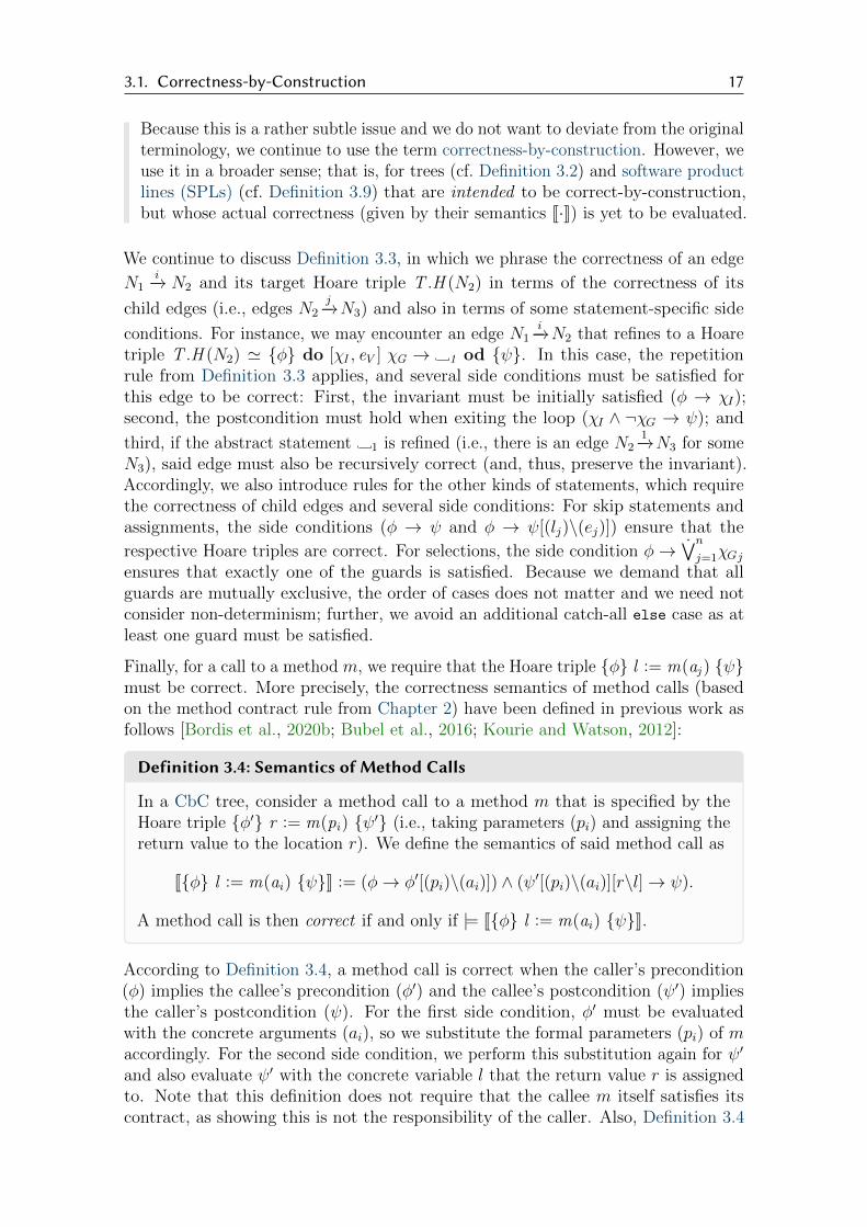
Finally, for a call to a method m, we require that the Hoare triple {φ} l := m(aj ) {ψ}must be correct. More precisely, the correctness semantics of method calls (basedon the method contract rule from Chapter 2) have been defined in previous work asfollows [Bordis et al., 2020b; Bubel et al., 2016; Kourie and Watson, 2012]:
Definition 3.4: Semantics of Method Calls
In a CbC tree, consider a method call to a method m that is specified by theHoare triple {φ′} r := m(pi) {ψ′} (i.e., taking parameters (pi) and assigning thereturn value to the location r). We define the semantics of said method call as
J{φ} l := m(ai) {ψ}K := (φ→ φ′[(pi)\(ai)]) ∧ (ψ′[(pi)\(ai)][r\l]→ ψ).
A method call is then correct if and only if |= J{φ} l := m(ai) {ψ}K.
According to Definition 3.4, a method call is correct when the caller’s precondition(φ) implies the callee’s precondition (φ′) and the callee’s postcondition (ψ′) impliesthe caller’s postcondition (ψ). For the first side condition, φ′ must be evaluatedwith the concrete arguments (ai), so we substitute the formal parameters (pi) of maccordingly. For the second side condition, we perform this substitution again for ψ′
and also evaluate ψ′ with the concrete variable l that the return value r is assignedto. Note that this definition does not require that the callee m itself satisfies itscontract, as showing this is not the responsibility of the caller. Also, Definition 3.4
18 3. Concept
JT K (1)
⇒ J 1© 1−→ 2©K (2)
⇒ J 2© 1−→ 3©K ∧ J 2© 2−→ 4©K (3)
⇒ (φ→ χM [i, A′, A′[len(A′)− 1]\0, new int[len(A) + 1], x]) ∧ J 2© 2−→ 4©K (4)
⇒ (χM → χI) ∧ (χI ∧ ¬χG → ψ) ∧ J 4© 1−→ 5©K (5)
⇒ χI ∧ χG → (χI ∧ 0 ≤ eV ∧ eV < (eV )old)[A′[i], i\A[i], i+ 1] (6)
Figure 3.2: Logical derivation for the correctness of the CbC tree in Figure 3.1.
neither formalizes the nature of methods, nor does it relate to SPLs in any way.This is why we revise this definition in Section 3.2, where we describe the precisemechanics of method contracting in the variability scenario. For the remainder ofthis section, we only consider CbC trees without any method calls.
Returning to the discussion of Definition 3.3, the correctness of an entire tree isgiven by the correctness of the edge at the root node, if any. Note that, whenever anabstract statement i in the Hoare triple of a node N1 is unrefined (i.e., there is no
edge N1i−→N2 for any N2), we consider said edge to be correct anyway (as in that
case, the universal quantification over an empty set in the definition of N1i−→∗ is
vacuously true). Thus, an incomplete CbC tree may be correct as well; in particular,the trivial CbC tree with only one root node and no edges is considered correct. Thisway, we also incorporate the incremental nature of CbC, where nodes and edges areadded successively to a tree; and we can keep evaluating the tree’s correctness, evenwhen it is not complete yet.
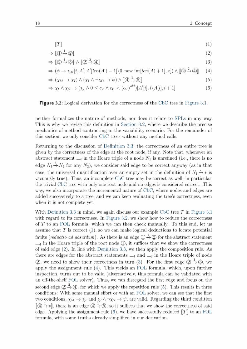
With Definition 3.3 in mind, we again discuss our example CbC tree T in Figure 3.1with regard to its correctness. In Figure 3.2, we show how to reduce the correctnessof T to an FOL formula, which we can then check manually. To this end, let usassume that T is correct (1), so we can make logical deductions to locate potential
faults (reductio ad absurdum). As there is an edge 1© 1−→ 2© for the abstract statement
1 in the Hoare triple of the root node 1©, it suffices that we show the correctnessof said edge (2). In line with Definition 3.3, we then apply the composition rule. Asthere are edges for the abstract statements 1 and 2 in the Hoare triple of node
2©, we need to show their correctness in turn (3). For the first edge 2© 1−→ 3©, weapply the assignment rule (4). This yields an FOL formula, which, upon furtherinspection, turns out to be valid (alternatively, this formula can be validated withan off-the-shelf FOL solver). Thus, we can disregard the first edge and focus on the
second edge 2© 2−→ 4©, for which we apply the repetition rule (5). This results in threeconditions: With some manual effort or with an FOL solver, we can see that the firsttwo conditions, χM → χI and χI ∧¬χG → ψ, are valid. Regarding the third condition
J 4© 1−→∗K, there is an edge 4© 1−→ 5©, so it suffices that we show the correctness of saidedge. Applying the assignment rule (6), we have successfully reduced JT K to an FOLformula, with some truths already simplified in our derivation.
3.1. Correctness-by-Construction 19
When we attempt to validate the remaining formula (6) (manually or with an FOLsolver), we finally find a hint at the mistake we made in Section 3.1.1. That is, whenwe simplify the formula (6) and omit all unrelated parts, we arrive at
i ≤ len(A)→ (i ≤ len(A))[i\i+ 1]
⇔ i ≤ len(A)→ i < len(A),
which is not valid (as a counterexample, consider the case i = len(A)). This resultsuggests that there may be a fault in the last loop run (i.e., when i = len(A)), whichis indeed where a buffer overflow occurs. We can now identify the bug, namely thatthere is one more iteration than intended in our loop, and fix it by defining theguard as χG := i < len(A) instead. With this change, our derivation (1)–(6) remainsunaffected and, evaluating the formula (6) again, we arrive at i < len(A) → (i ≤len(A))[i\i + 1], which is valid. In fact, the omitted remainder of the formula (6)is also valid with the corrected definition of χG. As our logical derivation can beperformed in a similar fashion in reverse direction, we can deduce that the correctedversion of our CbC tree is indeed correct in the sense of Definition 3.3.
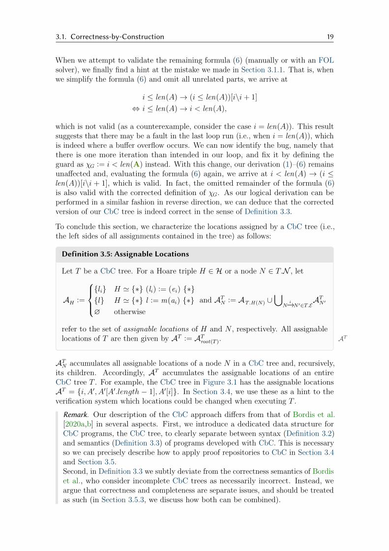
To conclude this section, we characterize the locations assigned by a CbC tree (i.e.,the left sides of all assignments contained in the tree) as follows:
Definition 3.5: Assignable Locations
Let T be a CbC tree. For a Hoare triple H ∈ H or a node N ∈ T.N , let
AH :=
{li} H ' {∗} (li) := (ei) {∗}{l} H ' {∗} l := m(ai) {∗}∅ otherwise
and ATN := AT .H (N) ∪⋃
Ni−→N ′∈T.E
ATN ′
refer to the set of assignable locations of H and N , respectively. All assignablelocations of T are then given by ATAT := ATroot(T ).
ATN accumulates all assignable locations of a node N in a CbC tree and, recursively,its children. Accordingly, AT accumulates the assignable locations of an entireCbC tree T . For example, the CbC tree in Figure 3.1 has the assignable locationsAT = {i, A′, A′[A′.length − 1], A′[i]}. In Section 3.4, we use these as a hint to theverification system which locations could be changed when executing T .
Remark. Our description of the CbC approach differs from that of Bordis et al.[2020a,b] in several aspects. First, we introduce a dedicated data structure forCbC programs, the CbC tree, to clearly separate between syntax (Definition 3.2)and semantics (Definition 3.3) of programs developed with CbC. This is necessaryso we can precisely describe how to apply proof repositories to CbC in Section 3.4and Section 3.5.Second, in Definition 3.3 we subtly deviate from the correctness semantics of Bordiset al., who consider incomplete CbC trees as necessarily incorrect. Instead, weargue that correctness and completeness are separate issues, and should be treatedas such (in Section 3.5.3, we discuss how both can be combined).

20 3. Concept
Third, we depart from the descriptions of Dijkstra [1975] and Kourie and Watson
[2012] in that we assume mutually exclusive selection cases using∨
; that is, it isalways clearly identifiable which case of a selection is executed, contrary to theoriginally proposed non-deterministic behavior. This facilitates our reasoning inSection 3.4 and is only a minor restriction, as two overlapping guards χG1 andχG2 can be easily rewritten to be mutually exclusive (e.g., to χG1 and ¬χG1 ∧ χG2,which gives χG1 preference over χG2).

3.2. Correct-by-Construction So�ware Product Lines 21
3.2 Correct-by-Construction So�ware Product Lines
In Section 3.1, we discussed how to represent a program as a CbC tree. However, aswe aim to check large programs with several methods (i.e., program units that maycall each other), we must consider how several CbC trees can be assembled to forman SPL. In addition, we must characterize when such an SPL is correct, building onour definition of correct CbC trees. To do so, we introduce two new concepts in thissection: First, we precisely define methods, which encapsulate CbC trees in a waythat enables method calls. Second, we describe how a feature model and a set ofinterconnected methods may form a correct-by-construction software product line(CSPL). For both concepts, we separate syntax (which is easily enforceable with toolsupport) and semantics (where the actual verification effort lies), as we already didfor CbC trees. Our descriptions in this section are only loosely based on those byBordis et al. [2020b], as we go into more detail regarding the semantics of methodsand CSPLs and put less emphasis on different contract composition mechanisms.
3.2.1 Syntax of Methods and CSPLs
We begin by introducing signatures, which we use throughout our formalizationto uniquely address methods and other program elements such as fields and imple-mentations. In particular, we use signatures as a common ground for CSPLs andproof repositories (cf. Section 3.3), which facilitates our combination of the two inSection 3.4 and Section 3.5.
Definition 3.6: Signature
A signature SS consists of a type S.type, a class name S.className, a nameS.name, and parameters S.(pi)
ni=0. A parameter pp = t n consists of a type t and
a name n. Where the names of parameters are irrelevant, we omit them.Two signatures S and S ′ are compatible if and only if S.type = S ′.type andS.(pi)
ni=0 = S ′.(pi)
ni=0 (ignoring the names of parameters).
For convenience, we introduce the notation S.type S.className::S.name(S.(pi))to completely specify a signature S.We refer to the set of all signatures as SS.
For example, the signature boolean Transaction::transfer(Account src, Account dst,int amount) may refer to a method named transfer in a class named Transactionthat returns a boolean and takes three parameters. This signature is compatible withthe signature boolean Transaction::instantTransfer(Account from, Account to, intmoney), but not with the signature boolean Transaction::instantTransfer(int money,Account from, Account to), because the parameter types do not match. Signaturescan also have empty class names, which we denote as S.type ::S.name(S.(pi)).
With signatures, we can formalize methods, which equip a CbC tree with a signatureand constrain the use of variables inside the tree. Thus, a method (as definedhere) loosely corresponds to a Java method in that it takes parameters, performs acomputation, and returns a value.

22 3. Concept
Definition 3.7: Syntax of Methods
A methodM M consists of a signature M.S = M.S.type ::M.S.name(M.S.(pi)), aset of local variables M.L, and a CbC tree M.T . A local variableL L = t n ∈M.Lconsists of a type t and a name n.All variables referenced in M.T must be declared, that is, they must refer toa local variable in M.L, to a parameter in M.S.(pi), or to the special returnvariable with type M.S.type and name� �.All original calls l := original(ai) in M.T and all original calls originalpre(ai)or originalpost(ai) in conditions must conform to the return type M.S.type andparameters M.S.(pi).A method M is complete if and only if its CbC tree M.T is complete.We refer to the set of all methods asM M.
Remark. As a succinct notation, we write M = (S � S ′,L � L′, T � T ′) todenote a method M with M.S = S ′, M.L = L′, and M.T = T ′. That is, weconsider M to be an unordered tuple whose elements (or values) can be accessed byname (or key) with a dot notation. We continue to use this notation throughout thethesis for other data structures as well. To extract all values for a given key kj froma set of such tuples X , we use the projectionπkj (X ) πkj (X ) := {vj | (ki � vi)
ni=1 ∈ X}
(e.g., πy({(x� i, y � 2i)}3i=1) = {2, 4, 6}) [Codd, 1970].
In Definition 3.7, the signature M.S of a method M has an empty class name, aswe consider all methods to exist in a single shared (classless) namespace, whichfacilitates our reduction to proof repositories in Section 3.4. This is not a restrictionwith regard to object-oriented programming (OOP), as instance methods can stillbe emulated by passing a this reference as the first argument of a method (onlyinheritance and late-binding polymorphism cannot be easily emulated, which wedisregard anyway in this thesis).
To exemplify Definition 3.7, we encapsulate the CbC tree T from Figure 3.1 as amethod MInsert (cf. Figure 3.3) by providing a name (Insert), defining parameters(A and x) and the loop variable (i), and by designating A′ as the return variable(denoted as a substitution T [A′\�]). We use T as it is given in Figure 3.1, includingthe faulty guard definition (χG := i < len(�) instead of the correct χG := i < len(A)).On its own, MInsert is not particularly useful; however, we embed it into a CSPL anddescribe how it interacts with other methods below.
(S � int[] ::Insert(int[] A, int x),
L � {int i},T � T [A′\�])
Figure 3.3: Example method MInsert that inserts an integer x into a list A (using theCbC tree T from Figure 3.1).

3.2. Correct-by-Construction So�ware Product Lines 23
First, we discuss how Definition 3.7 relates to the feature-oriented programming(FOP) paradigm as well as contract composition. To implement both, we allowmethods to use the special original keyword in two ways, which we refer to asoriginal calls in Definition 3.7: First, a method M may use the original keyword inany statement in M.T to call its original method as defined in FOP, which dependson the current configuration in a CSPL. We model this usage of original as a specialcase of the method call statement l := m(ai) where m = original . Second, M mayuse original in any pre- or postcondition in M.T to invoke the contract of its originalmethod. To denote whether we want to invoke the precondition φ or postconditionψ of its original method, we write originalpre or originalpost , respectively (to matchboth usages, we write original∗). Intuitively, we can model this usage of originalas FOL predicates originalpre(ai) and originalpost(ai) that are satisfied if and only ifφ[M.S.(pi)\(ai)] or ψ[M.S.(pi)\(ai)] are satisfied, respectively. To make this intuitionmore precise, we proceed to describe the external signatures that a method calls.
Definition 3.8: External Signatures
Let M be a method. With SMorigSMorig := M.S.type M.S.name::original(M.S.(pi)) and
SM (. . .)SM (l := m(ai)ni=0) := typeof (l) M.S.name::m(typeof (ai))
ni=0, we refer to the
signature of an original call and a method call in M , respectively, where typeof (·)denotes the types of the return variable and arguments.For a condition χ, a Hoare triple H ∈ H, and a node N ∈M.T.N , let
SMχ :=
{{SMorig} χ[original∗(ai)\] 6= χ
∅ otherwise,
SMH :=
{SMφ ∪ SMψ ∪ {SM (l := m(ai))} H ' {φ} l := m(ai) {ψ}SMφ ∪ SMψ H ' {φ} ∗ {ψ}, and
SMN := SMM .T .H (N) ∪⋃
Ni−→N ′∈M.T.E
SMN ′
refer to the set of external signatures of χ, H, and N , respectively. All externalsignatures of M are then given by SMSM := SMroot(M.T ). Further, we define the
external method signatures SMmethodSMmethod by substituting the highlighted set with ∅.
Definition 3.8 describes how a method interfaces with other methods via method andoriginal calls. That is, SMN accumulates all external signatures of a node N in theCbC tree of a method M and, recursively, its children (similar to Definition 3.5). Tothis end, every original call in a contract or statement as well as every regular methodcall is transformed into a signature with SMorig or SM (l := m(ai)
ni=0), respectively.
For example, suppose a method M with the signature float ::cos(float) contained amethod call s := sin(theta) such that both s and theta are floats, SM would containthe signature float cos::sin(float) (i.e., cos calls a method named sin that takesand returns a float). Similarly, suppose the same method contained an original calloriginal(theta), originalpre(theta), or originalpost(theta) such that theta is a float,SM would contain the signature float cos::original(float). Note that for our examplemethod MInsert in Figure 3.3, SMInsert = ∅ because MInsert does not contain anymethod or original calls. Below, we use the external signatures of a method to

24 3. Concept
look up the concrete methods that should be called, which depend on the currentconfiguration in a CSPL.
Next, we formally introduce CSPLs, which essentially comprise a feature modeland a collection of methods that may call each other. Note that the remark fromSection 3.1 still applies: A CSPL may be correct-by-construction by name; however,in this thesis we first consider it as allegedly “correct-by-construction” until we canconfirm or refute its correctness with our semantics.
In the following,2A 2A refers to the power set of a set A (i.e., the set of all subsets of A).
Definition 3.9: Syntax of CSPLs
A CSPLPL PL consists of a set of features PL.F , a set of configurations PL.C ⊆ 2PL.F ,a feature order≺PL ≺PL ⊆ PL.F ×PL.F , and a set of methods PL.M⊆ {F M | F ∈PL.F ,M ∈ M}, whereF M F M := (S � M.S.type ::F M.S.name(M.S.(pi)),L�M.L, T �M.T ) scopes a method M to a feature F .A CSPL must then satisfy the following properties:
1. ≺PL must be a strict total order (i.e., features can be uniquely linearized).
2. For any methods F1 M1, F2 M2 ∈ PL.M with M1.S.name = M2.S.name,M1.S must be compatible with M2.S (i.e., no overloading of signatures).
3. For any methods F M1, F M2 ∈ PL.M with M1 6= M2, M1.S 6= M2.S (i.e.,a signature may be implemented only once).
4. For any method F M ∈ PL.M, every assignable location in AM.T must referto a local variable in M.L or to � (i.e., all methods must be pure).
Definition 3.9 encodes the feature model of an SPL as a set of features together witha set of configurations. A configuration is simply a set of features that are selectedand whose methods should all be added to the corresponding product. Severalrepresentations for feature models are known in the literature, including featurediagrams, propositional formulas, and grammars [Apel et al., 2013a; Batory, 2005;Kang et al., 1990]. All of these representations can be reduced to the above form(e.g., with a SAT solver [Mendonca et al., 2009]). Thus, Definition 3.9 is compatiblewith several representations of feature models. The implementations of an SPL arethen given by a set of methods (cf. Definition 3.7), where we choose the methodnames so that they always begin with a feature they belong to.
Further, we require a feature order so that we can implement the FOP paradigm andcontract composition (1). Regarding the set of methods, we forbid overloading (2)and non-determinism (3), as we do not need the latter and can emulate the formerby renaming methods. Finally, we require that all methods are pure and do nothave any side effects (4), which allows us to disregard assignable locations whenmethods interact. That is, in our formalization, any method may internally haveund use assignable locations to perform its calculation; however, it may not affectany locations in other methods. We argue that this assumption is reasonable, as thetreatment of assignable locations is already sufficiently complex on its own [Engel

3.2. Correct-by-Construction So�ware Product Lines 25
et al., 2009]. Also, this assumption does not affect the approach by Bordis et al.[2020b], who also do not consider methods with side effects.
In Figure 3.4, we show an example CSPL for an SPL of list data structures and theiralgorithms. Our example is inspired by the graph product line [Lopez-Herrejon andBatory, 2001] and previous case studies on integer lists [Bordis, 2019; Kodetzki, 2020;Scholz et al., 2011]. In this CSPL, we consider three features List, Ordered, and Set (inthat order). The List feature represents an unordered list data type and its algorithms,while the Ordered and Set features provide specialized algorithms for ordered listsand mathematical sets (i.e., lists that eliminate any duplicates). We model the Listfeature as mandatory because it should implement general list algorithms and, thus,acts as a base feature. Accordingly, we only consider configurations that include thisfeature. We therefore arrive at four possible configurations in this CSPL, representingdifferent data types: unordered integer lists ({List}), integer lists in ascending order({List,Ordered}), unordered integer sets ({List, Set}), and integer sets in ascendingorder ({List,Ordered, Set}).
Besides the feature model, which is characterized by features and configurations,we consider three methods in this CSPL: First, the Insert method should insert aninteger into a given integer list and return the resulting list. Second, the Searchmethod should return whether an integer occurs in a given integer list. The lastmethod Sort should sort a given list and return the resulting list. Each feature in theCSPL may (but does not have to) implement these methods. In Figure 3.5, we showin a collaboration diagram [Reenskaug et al., 1992; Smaragdakis and Batory, 2002]which feature (given as columns) implements which methods (given as rows). Wemark unimplemented methods with × and visualize all intuitively possible originaland method calls with red and blue edges, respectively (we formalize this moreprecisely in Section 3.2.2). The implemented methods correspond to those given inFigure 3.4, which we proceed to discuss in more detail, with particular emphasis onmethod and original calls. We adapt some methods from Kourie and Watson [2012]as indicate in Figure 3.4. Further, we omit detailed CbC trees, which are constructedanalogously to Figure 3.1, and show only GCL statements.
As for the individual methods, the List feature implements both Insert and Search,but not Sort, which is irrelevant for unordered lists. List Insert corresponds toour example method MInsert from Figure 3.3 and performs ordinary list insertion,which involves no calls. List Search also does not involve any calls and implementsthe FOL predicate app with a linear search algorithm. Next, the Ordered featureimplements all three methods. In Ordered Insert, we take the obvious (if inefficient)route to implement insertion on ordered lists; that is, we simply append the newelement and sort the list thereafter. This involves two calls: original(A, x) to appendthe element and Sort(�) to sort the list. As for the contract of Ordered Insert, wewant to enrich the contract for List Insert with the assumption (and guarantee)that the supplied (and returned) lists are in ascending order. To this end, we calloriginalpre(A, x) in the pre- and originalpost(A, x) in the postcondition and conjointhese calls with the helper predicate isSorted, which can be implemented in FOLsuch that isSorted(A) if and only if the integer list A is sorted in ascending order.This particular usage of original∗ in a contract is an instance of behavioral subtyping(also known as Liskov substitution principle), as we weaken the precondition of

26 3. Concept
(F � {List,Ordered, Set},
C � {{List}, {List,Ordered}, {List, Set}, {List,Ordered, Set}},
≺ � {(List,Ordered), (Ordered, Set), (List, Set)},
M� {(S � int[] ::List Insert(int[] A, int x),
L � {int i},T � {len(A) > 0}
T [A′\�] (cf. Figure 3.3)
{len(�) = len(A) + 1 ∧ app(�, x) ∧ appAll(�, 0, len(A), A)}),
(S � boolean ::List Search(int[] A, int x),
L � {. . .},T � {len(A) > 0}
. . . (cf. Kourie and Watson [2012, p. 56ff.])
{� = true ↔ app(A, x)}),
(S � int[] ::Ordered Insert(int[] A, int x),
L � ∅,T � {originalpre(A, x) ∧ isSorted(A)}
� := original(A, x)
� := Sort(�){originalpost(A, x) ∧ isSorted(�)}),
(S � boolean ::Ordered Search(int[] A, int x),
L � {. . .},T � {originalpre(A, x) ∧ isSorted(A)}
. . . (cf. Kourie and Watson [2012, p. 66ff.])
{originalpost(A, x)}),
(S � int[] ::Ordered Sort(int[] A),
L � {int[] B, int[] C, . . .},T � {len(A) > 0} (cf. Kourie and Watson [2012, p. 191ff.])
. . . B, C := Sort(A[0,len(A)/2)), Sort(A[len(A)/2,len(A))) . . .
{appAll(A, 0, len(�), �) ∧ appAll(�, 0, len(A), A) ∧ isSorted(�)}),
(S � int[] ::Set Insert(int[] A, int x),
L � {boolean found},T � {originalpre(A, x) ∧ isSet(A)}
found := Search(A, x)
if found = true → � := A
found = false → � := original(A, x) fi
{(app(A, x)→ � = A)
∧ (¬app(A, x)→ originalpost(A, x)) ∧ isSet(�)})})
Figure 3.4: Example CSPL that models several kinds of list data structures.

3.2. Correct-by-Construction So�ware Product Lines 27
List Ordered SetInsert List Insert Ordered Insert Set Insert
Search List Search Ordered Search ×Sort × Ordered Sort ×
Figure 3.5: Collaboration diagram for the CSPL in Figure 3.4. Each edge denotesthe potential source and target of an original (red) and method (blue) call.
Ordered Insert and strengthen its postcondition [Liskov and Wing, 1994]. Thispattern (establishing behavioral subtyping by enriching contracts) is typical fororiginal calls in contracts [Thum et al., 2019]. Such usages of original∗ in contractsavoid code duplication in contracts and allow to express tailored, configuration-specific contracts, a technique that is known as contract composition [Thum et al.,2019]. In this thesis, we focus on explicit contract refinement, which allows a contractto invoke original∗ arbitrarily. Next, Ordered Search also uses similar original calls toinherit the contract of List Insert. Because we make the further assumption that thesupplied list is in ascending order, we implement this method more efficiently with abinary search algorithm. As this algorithm does not use a linear search approach,Ordered Search does not contain an original call in its CbC tree, only in its contract.In Figure 3.5, we draw a dashed edge between Ordered Search and List Search toshow that the former calls the latter only in its contract, not in its CbC tree, whichwill come into play in Section 3.2.2. The last method implemented by the Orderedfeature, Ordered Sort, sorts a given list in ascending order using the merge sortalgorithm to establish the isSorted predicate. It is specified to take any non-emptylist and return a list with the same elements in ascending order. Note that merge sortis a recursive algorithm; thus, Ordered Sort contains two calls to Sort to recursivelysort both halves of the supplied list, which we draw as a loop in Figure 3.5.
Finally, the Set feature implements only a single method, Set Insert, because Searchon sets is identical to Search on lists and Sort is irrelevant for sets. Similar toOrdered Insert, we again enrich the original contract with another assumption (andguarantee), namely that the supplied (and returned) lists are, in fact, sets. Thatis, the helper predicate isSet can be implemented in FOL such that isSet(A) ifand only if the integer list A does not contain any duplicates. In Figure 3.5, weshow that there are two possible targets for this original call (i.e., List Insert andOrdered Insert), depending on the configuration (i.e., whether Set Insert shouldoperate on unordered or ordered sets). This usage of original∗ is another instanceof explicit contract refinement as mentioned above. As for how to implement setinsertion, we simply check whether the new integer is already contained in the setwith a call to Search. If so (found = true), we can just return the set unchanged,otherwise (found = false) we invoke original to call List Insert and Ordered Insertas discussed above and insert the integer into the set. Depending on the result storedin found (which directly corresponds to app(A, x) in a logical context), we formalizethis fact as follows in the postcondition of Set Insert : If found = true, the set isunchanged (� = A), otherwise the original method must have been invoked and itspostcondition must hold (originalpost(A, x)). In either case, the result must be aset as well, according to the isSet predicate. Note that we cannot unconditionallyuse originalpost(A, x) in this postcondition, because the postcondition of List Insert
28 3. Concept
postulates that the resulting list is larger than before (len(�) = len(A) + 1), which isnot the case when a set already contains the element that is to be inserted.
The SPL in Figure 3.4 that consists of the features, configurations, and methodsdiscussed above is then, in fact, a CSPL according to the four properties in Defini-tion 3.9: The feature order is given by List ≺PL Ordered ≺PL Set (1), no methods areoverloaded or non-deterministic (2–3), and all methods assign at most their returnand local variables (4).
3.2.2 Semantics of Methods and CSPLs
With the example from Figure 3.4 at hand, we can examine the correctness ofmethods and entire CSPLs. Similar to CbC trees in Section 3.1, the example CSPLlooks plausible and satisfies all syntactic properties given in Definition 3.9. However,we have already seen that there is a fault in Figure 3.1, which we would like todetect and trace back to its original mistake at the method as well as product-linelevel. Already at the method level, this poses new challenges compared to plain CbCtrees: Intuitively, we may expect that a method M (according to Definition 3.7) iscorrect if and only if |= JM.T K (i.e., when its CbC tree is correct). However, thisonly works as intended when M does not contain any original or method calls (e.g.,for List Insert or List Search). In general, methods may call each other arbitrarilyat the product-line level; and we must consider this to evaluate the correctness of amethod.
To achieve this, a key observation is that the correctness of a method dependson the concrete methods referred to by its original and method calls. Above, wehave already seen that for a single method, there may be several candidates thatoriginal and method calls may refer to (e.g., in Figure 3.4, original in Set Insertmay call either List Insert or Ordered Insert, depending on the configuration). Byevaluating the correctness of a method in a CSPL for all possible candidates of itsoriginal and method calls, we can then derive the correctness of the method for allconfigurations in the CSPL. As a first step towards this goal, we introduce methodlookups, which map original and method calls to concrete methods that should becalled. By modifying the semantics of CbC trees, we then formalize when a methodis correct according to a given method lookup, as well as the precise mechanics ofcontract composition.
Definition 3.10: Semantics of Methods
Let PL be a CSPL. A method lookup for PL is a partial function` ` : S 7→ PL.Msuch that for any S ∈ S where `(S) is defined, `(S).S is compatible with S.We write `(S) = F M to state that `(S) is defined and maps to some methodF M ∈ PL.M. For a method lookup `, any method F M ∈ PL.M, and somepre- and postconditions φ and ψ, we evaluate whether all references to original∗in φ and ψ can be looked up with ` using
`F Mφ,ψ `F Mφ,ψ := (φ[original∗(ai)\] = φ) ∧ (ψ[original∗(ai)\] = ψ)
∨ `(SF Morig ) = F ′M ′ ∧ Hroot(M
′.T ) ' {φ′} ∗ {ψ′} ∧ `F ′ M ′
φ′,ψ′

3.2. Correct-by-Construction So�ware Product Lines 29
and we perform contract composition on a condition χ with
χF M`χF M` := (χ[original∗(ai)\] = χ) ∧ χ
∨ `(SF Morig ) = F ′M ′ ∧ Hroot(M
′.T ) ' {φ′} ∗ {ψ′}
∧ χ[originalpre(ai)\(φ′[M ′.S.(pi)\(ai)])F′ M ′
` ]
[originalpost(ai)\(ψ′[M ′.S.(pi)\(ai)])F′ M ′
` ].
By threading F M and ` through the correctness formulas from Definition 3.3,we arrive at the following modified definitions for the semantics of CbC trees:
JN1i−→N2KF M
`
:= T .H (N2) ' {φ} skip {ψ} ∧ (`F Mφ,ψ ∧ φF M
` → ψF M` )
∨ T .H (N2) ' {φ} (lj ) := (ej ) {ψ} ∧ (`F Mφ,ψ ∧ φF M
` → (ψF M` )[(lj)\(ej)])
∨ T .H (N2) ' {φ} l := m(aj ) {ψ} ∧ J{φ} l := m(aj ) {ψ}KF M`
∨ T .H (N2) ' {∗} 1 {∗} ∧ JN21−→∗KF M
`
∨ T .H (N2) ' {∗} 1 [χM ] 2 {∗} ∧ JN21−→∗KF M
` ∧ JN22−→∗KF M
`
∨ T .H (N2) ' {φ} if (χGj → j )nj=1 fi {∗}
∧ (`F Mφ,ψ ∧ φF M
` →∨n
j=1χGj) ∧
∧n
j=1JN2
j−→∗KF M`
∨ T .H (N2) ' {φ} do [χI , eV ] χG → 1 od {ψ}
∧ (`F Mφ,ψ ∧ φF M
` → χI) ∧ (`F Mφ,ψ ∧ χI ∧ ¬χG → ψF M
` ) ∧ JN21−→∗KF M
` ,
JN1i−→∗KF M
` :=∧
N2∈T.N ,N1i−→N2∈T.E
JN1i−→N2KF M
` , and
JT KF M` := Jroot(T )
1−→∗KF M` .
Similarly, we redefine the semantics of method calls (cf. Definition 3.4) as
J{φ} l := m(ai) {ψ}KF M`
:= `(SF M (l := m(ai))) = F ′M ′ ∧ Hroot(M′.T ) ' {φ′} ∗ {ψ′} ∧ `F M
φ,ψ ∧ `F′ M ′
φ′,ψ′ →(φF M
` → (φ′[M ′.S.(pi)\(ai)])F′ M ′
` ) ∧ ((ψ′[M ′.S.(pi)\(ai)][�\l])F′ M ′
` → ψF M` ).
We define the semantics of a method F M ∈ PL.M for a given method lookup `as JF MK`JF MK` := JF M.T KF M
` . F M is then `-correct if and only if |= JF MK`.
According to Definition 3.10, a method F M in a CSPL may be correct only withregard to a method lookup `; that is, it may be `-correct. The method lookup ` mapssome external signature S of F M (i.e., an original or method call) to some othermethod F ′M ′ in the CSPL. We then use ` to substitute calls with the signatureS in F M with the concrete contract of F ′M ′ to implement the explicit contractrefinement scheme described by Thum et al. [2019].
To this end, we modify Definition 3.3 to take F M and ` as indices. We highlight allthe new additions in red and proceed to discuss them in detail.

30 3. Concept
To perform contract composition (i.e., substitute occurrences of original∗ in contracts),we make use of the FOL formulas `F M
φ,ψ , φF M` , and φF M
` as follows: First, we conjoin`F Mφ,ψ to the antecedent of every side condition in Definition 3.3. This formula
is satisfied when either the contract does not contain the original keyword (i.e.,(φ[original∗(ai)\] = φ) ∧ (ψ[original∗(ai)\] = ψ)) or the signature associated withoriginal is bound to some method F ′M ′, in which case `F
′ M ′
φ′,ψ′ must be satisfiedrecursively for the contract of F ′M ′ (that is, the entire chain of original calls mustbe defined in `). Thus, for any side condition to be “activated”, all original calls inthe pre- and postcondition of a node’s Hoare triple (if any) must resolve to a concretemethod. Otherwise (i.e., `F M
φ,ψ is not satisfied), the side condition is vacuously truebecause ` does not carry enough information to (dis-)prove the side condition. Whena side condition is activated, we perform the actual contract composition with arecursion scheme similar to `F M
φ,ψ on the pre- and postcondition of a node’s Hoare tripleusing φF M
` and φF M` . That is, we substitute any contract occurrences of original∗
with the concrete pre- or postcondition of the method given by `. We also substituteany parameters (ai) accordingly and recursively substitute any other original calls as
well (with φ[originalpre(ai)\(φ′[M ′.S.(pi)\(ai)])F′ M ′
` ]). With these modifications, aside condition such as φ→ ψ for skip statements becomes `F M
φ,ψ ∧ φF M` → ψF M
` inDefinition 3.10, which is now aware of original calls and contract composition.
Finally, to evaluate the correctness of a method call l := m(ai) (where m may or maynot be original), we also modify the semantics of method calls given in Definition 3.4.Similar to above, we conjoin conditions to the antecedent of J{φ} l := m(ai) {ψ}KF M
` ,which states when a method call contributes to the correctness of the method:First, the method call must resolve to a concrete method according to ` (i.e.,SF M (l := m(ai)) = F ′M ′); second and third, all original calls in the contract ofF M as well as F ′M ′ must resolve to concrete methods as well (i.e., `F M
φ,ψ ∧ `F′ M ′
φ′,ψ′ ).As for the method contract rule, we modify it to take into account the contractcomposition scheme using φF M
` and ψF M` . Further, as we now consider methods and
not only plain CbC trees, we must take the parameters (M ′.S.(pi) instead of (pi))and return variable (� instead of r) into account.
Note that Definition 3.10 is a strict generalization of Definition 3.3, extending it witha proper treatment of original and method calls. That is, for any method F M thatdoes not contain any original or method calls (i.e., SF M = ∅), JF MK` ⇔ JF M.T Kfor any method lookup `. For instance, the method MInsert from Figure 3.3 is `-incorrect for any method lookup ` because it does not contain any calls and we havealready shown that its CbC tree (cf. Figure 3.1) is incorrect in Section 3.1.
To exemplify our treatment of original and method calls, we consider the `-correctnessof the method Ordered Insert (henceforth F M) from Figure 3.4. Regarding Fig-ure 3.5, we see that intuitively, we might map the original call to List Insert andthe method call to Ordered Sort with a method lookup (henceforth `). In Fig-ure 3.6a, we show the CbC tree of F M , which we omitted in Figure 3.4. ThisCbC tree comprises a composition of the original and method call with an inter-mediate condition χM . This intermediate condition calls originalpost(A, x), whichfollows as the postcondition of the original call and further functions as the precon-dition of the method call. χM also shows the reason why we distinguish originalpreand originalpost at all: Because χM acts as a pre- and postcondition to different

3.2. Correct-by-Construction So�ware Product Lines 31
{φ} 1 {ψ}
{φ} 1 [χM ] 2 {ψ}
� := original(A, x) � := Sort(�)
1
1 2
φ = originalpre(A, x) ∧ isSorted(A)
ψ = originalpost(A, x) ∧ isSorted(�)χM = originalpost(A, x)
(a) With unresolved original∗ calls
{φF M` } 1 {ψF M
` }
{φF M` } 1 [(χM )F M
` ] 2 {ψF M` }
� := original(A, x) � := Sort(�)
1
1 2
φF M` = len(A) > 0 ∧ isSorted(A)
ψF M` = ψList Insert ∧ isSorted(�)
(χM)F M` = ψList Insert
(b) With resolved original∗ calls
Figure 3.6: CbC trees for the method Ordered Insert in the CSPL from Figure 3.4.
Hoare triples, it is not obvious whether χM should invoke the pre- or postconditionof the original method. Thus, we explicitly annotate which condition we wantto invoke (if desired, this may be avoided with an arbitrary convention). In Fig-ure 3.6b, we show how the CbC tree in Figure 3.6a looks like when we substituteall occurrences of original∗ with their respective target methods according to Defini-tion 3.10 and ` as defined above. That is, we substitute originalpre(A, x) with theprecondition of List Insert (and originalpost(A, x) with its postcondition ψList Insert ,respectively). To determine whether F M is `-correct, it then suffices if we showthat |= J{φ} � := original(A, x ) {χM}KF M
` ∧ J{χM} � := Sort(�) {ψ}KF M` . By our
choice of `, the antecedents of both method calls are satisfied. With some manualeffort or an FOL solver, we can see that their consequents are satisfied as well. Intotal, this shows that Ordered Insert is correct when we map its original call toList Insert and its method call to Ordered Sort. Note that although the CbC tree forList Insert (cf. Figure 3.1) contains a fault, Ordered Insert is `-correct anyway. Thisis because the implementation of List Insert does not play a role when (dis-)provingthe correctness of Ordered Insert, which only relies on the contract of List Insert.
By now, we explained in detail how we can ascertain a method’s correctness withrespect to some method lookup. Up to now, we visualized all possible original andmethod calls in Figure 3.5 based on intuition, and chose a method lookup accordinglyfor our discussion of Ordered Insert. However, we have yet to show how precisely wechoose method lookups when we evaluate the correctness of an entire CSPL. Our ideafor this is naive, but accurate: We simply derive all products of a given CSPL andcheck whether they are all correct. Deriving a product amounts to determining whichmethods are included in it and how they call each other, which we describe witha method lookup `CPL. Checking a product’s correctness then amounts to checkingall its derived methods for `CPL-correctness. We proceed to formalize this idea moreaccurately.

32 3. Concept
Definition 3.11: Semantics of CSPLs
Let PL be a CSPL and C ∈ PL.C a configuration (or restriction thereof).≺PL induces a relation≺CPL ≺CPL with F1 ≺CPL F2 if and only if F1, F2 ∈ C ∧ F1 ≺PL
F2∧¬∨F ′∈C(F1 ≺PL F
′∧F ′ ≺PL F2) (i.e., F1 directly precedes F2 in C with respect
to the feature order ≺PL). Further,lastCPL(F ) lastCPL(F ) := F ∈ C ∧ ¬∨F ′∈CF ≺PL F ′
denotes whether F is the last feature in C with respect to the feature order ≺PL.In addition, we writeσ(. . .) σ(C, n) := {F ∈ C | F M ∈ PL.M,M.S.name = n} torestrict a configuration C to all features that implement a method named n.We then calculate the derived methods associated with C in PL with
∇(0)PL,C := {F M ∈ PL.M | last
σ(C ,M .S .name)PL (F )},
∇(i+1)PL,C :=
⋃F M∈∇(i)
PL,C
{F ′M ′ ∈ PL.M | SMorig ∈ SMmethod ,
F ′ ≺σ(C,M.S.name)PL F,M ′.S.name = M.S.name}, and
∇PL,C ∇PL,C :=⋃
i≥0∇(i)
PL,C .
Next, we define the method lookup`CPL `CPL such that for all F M ∈ PL.M andS ′ ∈ SF M , `CPL(S ′) := F ′M ′ ∈ PL.M if and only if
|= S ′.name = original ∧ F ′ ≺σ(C,M.S.name)PL F ∧M ′.S.name = M.S.name
∨ S ′.name 6= original ∧ lastσ(C ,S ′.name)PL (F ′) ∧M ′.S.name = S ′.name,
otherwise `CPL(S ′) is undefined.Finally, we define the semantics of PL as
JPLK JPLK :=∧
C∈PL.CF M∈∇PL,C
JF MK`CPL .
PL is then correct if and only if |= JPLK.
Thus, a CSPL PL is correct according to Definition 3.11 when for all its configurationsC ∈ PL.C every derived method in ∇PL,C is `CPL-correct (assuming a finite numberof methods in PL.M, ∇PL,C is finite as well). The calculation of ∇PL,C and `CPL isbest explained with a practical example. To this end, consider Figure 3.7, where wevisualize both calculations for all four configurations of the CSPL from Figure 3.4.In the following discussion, let PL refer to said CSPL and Mn ∈ PL.M to a methodsuch that M.S.name = n; thus, we are able to precisely refer to the method’s tuplein formal contexts below.
In Figure 3.7a, we show a collaboration diagram similar to Figure 3.5, this timespecifically for the configuration corresponding to an unordered integer list. Eachmethod in the CSPL corresponds to one cell of this diagram; again, we markunimplemented methods with ×. When evaluating the correctness of this particularconfiguration, we only have to consider certain methods in this diagram. Theset ∇PL,{List} characterizes these derived methods and we mark all methods thatbelong to ∇PL,{List} with , all others with # (and analogously for Figure 3.7b–3.7d).

3.2. Correct-by-Construction So�ware Product Lines 33
Lis
tO
rder
edSet
Insert # #
Search # ×Sort × # ×
(a) {List}
Lis
tO
rder
edSet
#
# ×× ×
(b) {List,Ordered}
Lis
tO
rder
edSet
#
# ×× # ×
(c) {List,Set}
Lis
tO
rder
edSet
# ×× ×
(d) {List,Ordered,Set}
Figure 3.7: Configuration-specific collaboration diagrams for the CSPL in Figure 3.4.
For this configuration, only the methods named List Insert and List Search arerelevant (i.e., ∇PL,{List} = {MList Insert ,MList Search}) and we can ignore all othermethods, as they do not belong to the derived product. In Figure 3.7b–3.7d, wealso show the sources and targets of original and method calls as edges (coloredred and blue, respectively), which directly correspond to the method lookup `CPLfor the respective configuration. In the case of Figure 3.7a, however, both derivedmethods do not contain any calls, so the method lookup `
{List}PL for this configuration
is empty (i.e., it does not map any signatures) and the collaboration diagram doesnot contain any edges. Thus, the configuration (and corresponding product) {List}is correct when |= JMList InsertK`{List}
PL∧ JMList SearchK`{List}
PLor, due to the lack of calls,
|= JMList Insert .T K ∧ JMList Search .T K.
For the other three configurations, matters are slightly more complicated becauseoriginal and method calls are involved. For instance, let us consider the configurationcorresponding to an integer list in ascending order, {List,Ordered}, which we show inFigure 3.7b. To calculate the derived methods ∇PL,{List,Ordered}, we use the followingapproach, which is an alternative phrasing of Definition 3.11: First, in each row ofthe collaboration diagram, we choose the rightmost cell whose feature is still selectedin the configuration and add the corresponding method to ∇PL,{List,Ordered}. Next, werepeatedly add cells to the left of cells that are already in ∇PL,{List,Ordered} if the formercell’s feature is selected and the method corresponding to the latter cell contains anoriginal call in its CbC tree. For this concrete configuration, that means we chooseall methods implemented by the feature Ordered, which are the rightmost cells whosefeature (Ordered) is still selected in {List,Ordered}. As Ordered Insert calls originalin its CbC tree, we also add List Insert to ∇PL,{List,Ordered}. However, we do not addList Search as a derived method, because Ordered Search does not call original inits CbC tree, only in its contract (i.e., SMOrdered Search
orig /∈ SMOrdered Searchmethod ). Intuitively, we
can explain this as follows: Whenever we call the method Ordered Insert in theproduct that the configuration {List,Ordered} represents, the method List Insertcan possibly be invoked as well through an original call. Thus, this method mustbe correct as well for the product to be correct and should therefore belong to theconfiguration’s derived methods. However, when we call Ordered Search, List Searchcan never be invoked at runtime, so any faults in its implementation will not affectthe derived product; therefore, we do not need to evaluate its correctness for thisproduct. In total, the derived methods for this configurations are then given by∇PL,{List,Ordered} = {MList Insert ,MOrdered Insert ,MOrdered Search ,MOrdered Sort}.
34 3. Concept
As for the method lookup `{List,Ordered}PL , Definition 3.11 utilizes a similar scheme
as for the derived methods to define mappings: Signatures for original calls aregenerally mapped to cells that are to the left of the current cell, while signaturesfor method calls are mapped to the rightmost cell whose feature is still selected inthe configuration (which represents the “frontend” of a method). For this concreteconfiguration, this method lookup is then given by
`{List,Ordered}PL : S 7→ PL.M
int[] Ordered Insert::original(int[] A, int x) 7→MList Insert
boolean Ordered Search::original(int[] A, int x) 7→MList Search
int[] Ordered Insert::Sort(int[] A) 7→MOrdered Sort
int[] Ordered Sort::Sort(int[] A) 7→MOrdered Sort .
The four mappings correspond to the colored edges in Figure 3.7b. Note that thecall to Sort in the method Ordered Sort is mapped recursively to Ordered Sort itself,which is also the intended behavior for correctly evaluating the merge sort algorithm.
The derived methods and method lookups for the remaining two configurations canbe determined analogously. In particular, note how for the configuration {List, Set},the methods implemented by the feature Ordered are completely skipped, as Or-dered is not selected in this configuration. Instead, both the original and methodcall in Set Insert are mapped directly to methods implemented by the featureList. Also note that the derived methods and method lookup for the configuration{List,Ordered, Set} generalize those of the configuration {List,Ordered} (i.e., Fig-ure 3.7b is completely contained in Figure 3.7d). This hints at some optimizationpotential, which we discuss below in more detail.
With our discussion of derived methods and method lookups completed, we canfinally evaluate the correctness of the CSPL from Figure 3.4. Above, we alreadynoted that the CbC tree for List Insert contains a fault (the faulty guard definitionfrom Figure 3.1), so we know for sure that 6|= JMList Insert .T K. We also observedthat JF MK` ⇔ JF M.T K for any method lookup ` whenever F M does not containany calls, so also 6|= JMList InsertK`CPL for any configuration C ∈ PL.C. RegardingFigure 3.7, we see that List Insert is a derived method for every configuration andmust therefore be correct, which it is not. Thus, the CSPL is incorrect as well. Notethat our definitions allow us to accurately locate the fault as follows: The CSPL isincorrect because each configuration is incorrect; each of which is incorrect becauseList Insert is incorrect; which is incorrect because the Hoare triple for node 5© inFigure 3.1 is incorrect. In Section 3.4, we discuss whether and how this kind ofbug tracking is also possible with our approach for combining CSPLs and proofrepositories (cf. Section 3.3).
To conclude this section, we briefly discuss how this approach for evaluating thecorrectness of CSPLs leaves room for improvement. When we consider Figure 3.7, wecan use the derived methods to deduce the number of `-correctness evaluations thatare necessary to evaluate the correctness of our entire example CSPL. That is, wehave to check two methods (i.e., List Insert and List Search) for the configuration{List}, four methods for {List,Ordered}, three methods for {List, Set}, and fivemethods for {List,Ordered, Set}. Note, however, that we have to check the method
3.2. Correct-by-Construction So�ware Product Lines 35
List Insert four times in total with essentially the same result, and the same goesfor the other methods (e.g., we check List Search twice). In the literature, thisapproach is also known as an unoptimized product-based analysis, as it essentiallychecks each configuration (or product) of the CSPL (and, thus, their methods) inisolation [Thum et al., 2014a]. Intuitively, this is redundant effort, and we wouldrather like to check each method only as often as it is absolutely required. Thus,this approach for evaluating CSPL correctness does not allow for proof reuse andhas significant potential for optimization.
In this section, we gave a detailed account on how to evaluate the correctness ofCSPLs in a product-based fashion. However, this procedure does not allow for anyproof reuse and is therefore inefficient for large CSPLs. The goal of our thesis isto determine whether and how this process can be accelerated. To this end, weintroduce a completely different idea, the proof repository, which has nothing to dowith CbC and CSPLs at the first glance (cf. Section 3.3), but lends itself well tochecking CSPLs on further inspection as described in Section 3.4 and Section 3.5.
Remark. Our description of CSPLs again differs from that of Bordis et al. [2020a,b],as we continue to enforce a clear separation between syntax (which is simpleto check) and semantics (which requires verification effort); a separation thatfacilitates our reasoning in Section 3.4 and Section 3.5. In addition, we introducesignatures (cf. Definition 3.6), which act as a common ground for CSPLs and proofrepositories. Another difference is that we focus on explicit contract refinementas described by Thum et al. [2019], while Bordis et al. also discuss conjunctivecontract refinement and contract overriding. As explicit contract refinement is ageneralization of both these techniques, this is not a restriction. In our formalizationof explicit contract refinement (cf. Definition 3.10), we further distinguish betweencalls to originalpre and originalpost to precisely specify which condition of a contractis to be substituted, which is necessary for original calls in intermediate conditions.Finally, we deliberately do not utilize previous formalizations for feature models(e.g., by Schobbens et al. [2006]) and FOP (e.g., GenVoca or AHEAD [Batory andO’Malley, 1992; Batory et al., 2004]). We do not formalize feature models becausethey are irrelevant to our approach, which only depends on the configurationsin a CSPL. Thus, we avoid lock-in to a specific feature modeling technique (e.g.,feature diagrams), while we can still consider the evolution of configurations (e.g.,as classified by Thum et al. [2009]). We further avoid a full formalization of FOP,which would unnecessarily complicate our definitions (e.g., the AHEAD focuses onnested and non-code artifacts, both of which are irrelevant in this thesis).

36 3. Concept
3.3 Proof RepositoriesThe technical foundation for how to accelerate the correctness evaluation of a CSPLis the proof repository (PR), a data structure that effectively caches previouslyconducted proofs to maximize proof reuse. The proof repository approach wasproposed by Bubel et al. [2016] as a means to improve performance of verification-in-the-large. In particular, Bubel et al. notice that many verification systems (e.g.,KeY, by default) make strict assumptions about the structure of programs. For thePhV use case, or when contracts are fixed beforehand and evolution only happenson the implementation-level, this may be acceptable. However, when consideringspecification-level evolution, such verification systems often require re-verifyingconsiderable parts of a program, especially when a specification change cascadesthrough the entire program. Furthermore, these verification systems do not offer theflexibility to verify an entire CSPL in a single or few passes; instead, all products ofa CSPL must be verified independently, which is infeasible for large CSPLs (as wediscussed in Section 3.1).
To improve support for both scenarios (i.e., evolution and variability), Bubel et al.utilize two ideas: First, abstract contracts permit to separate a method call from thecontract that is actually substituted by the method contract rule [Bubel et al., 2014;Hahnle et al., 2013]. This way, calls and called implementations are disentangled. Wefurther discuss abstract contracts and how they aid in checking CSPLs in Chapter 4.Second, proof repositories allow for systematic caching and reuse of “partial” proofs,that is, proofs that can be completed by substituting concrete contracts. Theflexibility of proof repositories allows for different use cases, such as late bindingand delta-oriented programming (DOP), which Bubel et al. briefly describe. InSection 3.4 and Section 3.5, we discuss how we adapt proof repositories to CbC andCSPLs, respectively.
In this section, we present revised formalizations and examples of the programmingmodel and proof repositories based on the description by Bubel et al. [2016]. Ourformalization differs from theirs in its presentation to allow for more concise definitionsand algorithms in our extensions for CbC and CSPLs. Most of our changes tothe formalization do not change the semantics of programs and proof repositories.However, some changes to the semantics were reasonable or even necessary, whichwe point out and justify.
3.3.1 Programming Model
The basic approach of Bubel et al. is to clearly separate a method call from theimplementation that is actually called. That is, when a verification system encountersa method call in a program, it should not immediately commit to a specific invokedimplementation (and substitute its contract with the method contract rule), butallow to defer the choice of the invoked implementation to a later point in time. Thisbears some semblance to late binding, a kind of polymorphism in OOP languageswhere the invoked implementation for a method call is only determined at runtime.However, while proof repositories can be used to implement late binding, they permitother binding strategies for method calls as well, so that proof repositories may beadapted to other programming paradigms (e.g., DOP, FOP, or, in this thesis, CbC).

3.3. Proof Repositories 37
To be able to explicitly track bindings from method calls to concrete implementations,Bubel et al. propose a programming model that allows any call to be bound to no,one, or many implementations. Based on the signatures we also use for CSPLs inDefinition 3.6, we formalize an abstracted view of a program in an OOP language asfollows:
Definition 3.12: Syntax of Programs
A program PP consists of a set of classes P.C and a set of bindings P.B. Let P besuch a program.A class CC ∈ P.C consists of a class name C.name, a set of fields C.F , and a set ofimplementations C.I. There shall be no two classes in P.C with the same name.In a class C, a field FF ∈ C.F is a signature F.type C.name::F.name withempty parameters. An implementation II ∈ C.I consists of a signatureI.S = I.S.type C.name::I.S.name(I.S.(pi)), three clauses I.requires, I.ensures,and I.assignable, as well as a body I.body . There shall be no two implementa-tions in C.I with the same signature. Let impls(P )impls(P ) :=
⋃C∈P.CC.I refer to all
implementations in all classes of P .A call cc consists of two signatures c.Sin ∈ πS (impls(P )) and c.Sto. A binding
BB ∈ P.B consists of a call B.src and a signature B.Sdst ∈ πS (impls(P )) such thatB.Sdst is compatible with B.src.Sto .We refer to the set of all programs as PP .
Like Bubel et al., we focus on Java programs and contracts that are specified withthe Java modeling language (JML) [Leavens and Cheon, 2006; Leavens et al., 1998].This way, we can implement and evaluate our concept with the KeY verificationsystem, which only supports Java and JML; however, our concept and definitionsare generalizable to other languages with similar concepts, such as C++ or C#. Forsimplicity, Definition 3.12 ignores many concepts from OOP languages: In particular,we do not consider inheritance hierarchies, field and implementation modifiers (e.g.,public or static), non-default constructors, generic data types, and exceptions; asthese are all not relevant to our concept.
In Figure 3.8, we show a simple example program P that allows customers to transfermoney between bank accounts. Our example is inspired by previous case studieson bank accounts [Thum et al., 2011, 2012a, 2014b]. The program comprises theclasses Account and Transaction with several fields and implementations, as well asthree bindings for calls in these implementations. The contract of an implementationis specified using its requires, ensures, and assignable clauses, which are expressedin JML. Typical JML keywords can be used, such as \result (to refer to the returnvalue), \old(. . .) (to refer to pre-state values), \nothing , and \everything (to specifyupdatable heap locations). To specify a trivial pre- or postcondition, true maybe used. The body of an implementation I can contain any valid Java code—forconstructing a proof repository, only the calls in I are relevant, not any otherstatements in the body. In Figure 3.8, the only implementation that has any calls isboolean Transaction::transfer(Account, Account, int), whose body contains calls withthe signatures boolean Account::update(int) and boolean Account::isLocked().

38 3. Concept
(C � {(name � Account,
F � {int Account::balance, boolean Account::lock},I � {(S �I1 boolean Account::update(int x),
requires � true,ensures � balance == \old(balance) + x && \result ,assignable � balance,body � balance = balance + x; return true;),
(S �I2 boolean Account::isLocked(),requires � true,ensures � \result == lock,assignable � \nothing ,body � return lock;),
(S �I3 boolean Account::lockDown(),requires � true,ensures � \result == true,assignable � \nothing ,body � return true;)}),
(name � Transaction,
F � ∅,I � {(S �I4 boolean Transaction::transfer(
Account src, Account dst, int amount),requires � src != dst && amount >= 0,ensures � \result ==> (\old(dst.balance) + amount ==
dst.balance && \old(src.balance) - amount ==src.balance),
assignable � \everything ,body � if (dst.isLocked() || src.isLocked())
amount = -1;
return amount >= 0 &&
src.update(-1 * amount) &&
dst.update(amount);)})},B � {(src � (Sin �B1B1 boolean Transaction::transfer(. . . ),
Sto � boolean Account::update(int)),Sdst � boolean Account::update(int)),
(src � (Sin �B2 boolean Transaction::transfer(. . . ),Sto � boolean Account::isLocked()),
Sdst � boolean Account::isLocked()),
(src � (Sin �B3 boolean Transaction::transfer(. . . ),Sto � boolean Account::isLocked()),
Sdst � boolean Account::lockDown())})
Figure 3.8: Example program that models bank accounts.

3.3. Proof Repositories 39
With a binding B, such a call (B.src) can be bound to a concrete implementation(B.Sdst). In our example, we choose to bind the call (Sin � boolean Transaction::transfer(. . . ), Sto � boolean Account::update(int)) to the only implementation witha compatible signature, that is, boolean Account::update(int). However, a call doesnot need to be bound to any implementation (i.e., it is unbound) and may also bebound to more than one implementation. For example, we choose to bind the call(Sin � boolean Transaction::transfer(. . . ), Sto � boolean Account::isLocked()) totwo implementations, which both have compatible signatures. This call is thereforenon-deterministic: Either boolean Account::isLocked() or boolean Account::lockDown()may be invoked during its execution. This is in contrast to the operation of a normalcompiler, which expects that a call statically resolves to exactly one implementation.
Note that Definition 3.12 does not prescribe any binding strategy; thus, it is applicablein different use cases, such as late binding, non-deterministic programming, andDOP. In our example, we use an arbitrary binding strategy (just for demonstrationpurposes) that binds every call to every implementation that has a compatiblesignature. When we construct a proof repository for this example in Section 3.3.3,this binding strategy will basically create two different proofs of boolean Transaction::transfer(. . . ): One where boolean Account::isLocked() is invoked (and bank accountscan be individually locked or unlocked, depending on the attribute boolean Account::lock), and another where boolean Account::lockDown() is invoked (and the entirebank is locked down, ignoring the attribute). Thus, by binding a call to multipleimplementations, we are able to represent variation; we leverage this to combineproof repositories with CSPLs in Section 3.4 and Section 3.5.
We proceed to precisely specify which calls an implementation comprises.
Definition 3.13: Direct and Extended Calls
Let P be a program and I ∈ impls(P ) an implementation. I calls a signature Sif and only if S occurs in I.requires , I.ensures , or I.body . I co-calls S if and onlyif S occurs in I.requires or I.ensures (i.e., S is called from within the contract ofI). We calculate the direct calls and extended calls for I and B ⊆ P.B with
calls(i)(I)calls (i)(I) := {(Sin � I.S, Sto � S) | S ∈ S,{I calls S i = 0
I co-calls S i > 0
}} and
calls(i)P (I,B)calls
(i)P (I,B) := calls(i)(I) ∪
⋃c∈calls(i)(I)
{c′ |B ∈ B, I ′ ∈ impls(P ), B.Sdst = I ′.S,
B.src = c, c′∈calls(i+1)P (I ′,B\{B})}.
Finally, let calls(P )calls(P ) :=⋃I∈impls(P )calls(0)(I) refer to all direct calls in P .
A program P is complete if and only if calls(P ) ⊆ πsrc(P.B).
In Definition 3.13, we distinguish two kinds of direct calls in an implementation I:Those that occur in the contract or body of I are calls and given by calls(0)(I), whilethose that occur only in the contract of I are co-calls and given by calls(i)(I) fori > 0. For example, both calls in boolean Transaction::transfer(. . . ) are direct calls(and no co-calls). When no co-calls are involved (as in our example), the extendedcalls simply correspond to the direct calls. However, when co-calls are involved (e.g.,

40 3. Concept
an original call in a CSPL), we may need to consider also some additional callsbesides the direct calls, which we refer to as extended calls. Formally, the recursivespecification of extended calls in Definition 3.13 is quite complicated. However,intuitively, the set of extended calls calls
(0)P (I,B) denotes which calls are relevant to
determine the correctness of an implementation I when we assume a set of bindingsB. Assuming an empty set of bindings, calls
(0)P (I,B) corresponds to the direct calls
calls(0)(I). However, when we bind a call to some implementation I ′ and apply themethod contract rule, the contract of I ′ may in turn contain a co-call, which weneed to bind again, possibly yielding another co-call, and so on. For example, withregard to CSPLs, consider the chain of original calls in Figure 3.7d: The contract ofSet Insert invokes original, which we may bind to Ordered Insert, which itself invokesoriginal, which we may finally bind to List Insert, where no original is invoked again.This shows how, when we bind an extended call, we might determine some newextended calls, which may then recursively be bound again. We demonstrate thisprinciple with a more detailed example when we combine proof repositories and CbCin Section 3.4. In simple scenarios (e.g., the example in Figure 3.8), no co-calls are
involved at all. Thus, calls(i)P (I,B) = calls(i)(I) for any B ⊆ P.B, so we need not
make a difference between direct and extended calls in such scenarios.
Remark. In the original formalization by Bubel et al. [2016], there is no signaturedefinition; instead they use labels to identify implementations. However, theirapproach is too restrictive, as calls cannot be bound freely to any compatiblesignature, which we require in Section 3.4. Further, Bubel et al. distinguish betweendifferent code positions of calls within an implementation: For example, bothcalls in the body if (dst.isLocked() || src.isLocked()) ...; can be boundindependently to different implementations using their approach. Because we donot require this flexibility in this thesis, we omit it and simplify the definitionsaccordingly. Finally, our notion of extended calls does not exist in the originalformalization by Bubel et al. This is because we explicitly address contractcomposition in CSPLs (which necessitates co-calls), while Bubel et al. onlyconsider direct calls.
3.3.2 Verification SystemThe defining feature of the programming model from Definition 3.12 is that itseparates method calls from implementations by means of bindings. To leveragethis separation for maximum proof reuse, the utilized verification system must havesupport for partial proofs; that is, it must be able to conduct a proof partially for animplementation even when some of its calls are still unbound. To characterize thisrequirement more precisely, we define a general interface for a proof-repository-capableverification system, without having to commit to a concrete implementation.
Definition 3.14: Verification System
Let P be a program. A verification system checks whether an implementationsatisfies all properties specified in its contract. More precisely, it checks for agiven implementation I ∈ impls(P ) whether
|= (I.requires → 〈I.body〉I.ensures) ∧ assigns(I.body , I.assignable). (3.7)

3.3. Proof Repositories 41
The assigns(·) predicate ensures that I.body modifies at most the locations givenin I.assignable, the details of which can be found in Engel et al. [2009, Def. 11].At any given time, the verification system has a verification state VV , whichencodes the current progress of an ongoing proof. We refer to the set of allverification states as VV .A verification system must offer three functions that operate on verification states:
• First, V = beginProofP(I) must begin a new proof by returning an initialverification state V ∈ V for a given implementation I ∈ impls(P ). Thisfunction may already verify all specified properties of the implementationthat do not rely on any calls in calls (0)(I). In particular, this function mayalready construct a complete proof when calls(0)(I) = ∅.
• Second, V ′ = continueProofP(V,B) must continue a proof given by a verifi-cation state V ∈ V , taking into account a new binding B ∈ P.B, and returna new verification state V ′ ∈ V. Thus, specified properties that rely on thenewly bound call B.src may be verified.
• Third, completeProof (V ) must attempt to complete a proof given by averification state V ∈ V and return whether formula (3.7) is valid. Thisfunction must attempt to verify all yet unverified specified properties andreturn false when it fails.
These three functions must be pure (i.e., they must return the same value for thesame arguments and must not have any side effects). In logical contexts, we maytherefore interpret the function completeProof (V ) as a DL formula JV KJV K, whichstates that completeProof (V ) returns true. A verification state V ∈ V is thenclosable (denoted as V 3V 3) if and only if |= JV K, otherwise it is open (denoted as
V 7V 7). Two verification states V1, V2 ∈ V are equivalent if and only if JV1K⇔ JV2K.Further, adding two bindings B1 and B2 shall commute up to equivalence ofverification states, that is,
JcontinueProofP(continueProofP(V,B1), B2)K⇔ JcontinueProofP(continueProofP(V,B2), B1)K.
(3.8)
In the following, we assume a fixed verification system.
With this definition, proof repositories can be clearly separated from a concreteverification system. In Chapter 4, we describe how to modify the KeY verificationsystem so that it conforms to this definition. Conceptually, a verification state Vcan be thought of as a set of open proof obligations (expressed as DL formulas):The function beginProof initializes a new proof, closes all proof obligations whichare already closable, and returns all remaining open proof obligations. The functioncontinueProof then utilizes the new binding to close proof obligations that are relatedto the newly bound call. Finally, the function completeProof attempts to close anyremaining proof obligations and returns whether V = ∅; if so, all proof obligationswere closed and formula (3.7) is valid. These functions must form a confluent systemas expressed by the property (3.8); that is, the order in which proofs are continueddoes not matter [Baader and Nipkow, 1998].

42 3. Concept
Remark. Bubel et al. [2016] propose abstract contracts to implement a proof-repository-capable verification system. However, their formalization does notclearly separate abstract contracts and proof repositories. We argue that abstractcontracts can be considered an implementation detail and our definition of averification system is an appropriate generalization that avoids an early commitmentto abstract contracts. We elaborate on this issue in Chapter 4.
3.3.3 Syntax and Semantics of Proof Repositories
With a programming model and verification system in place, we move towardsintroducing the proof repository, which is the main data structure proposed by Bubelet al. [2016] to achieve proof reuse. A proof repository maps descriptions of proofsthat should be conducted (represented by proof descriptors) to the actual proofs(represented by verification states from Definition 3.14). A proof can then be lookedup by its descriptor without any need for re-verification.
First, we specify proof descriptors, many of which form the proof repository domainfor a program.
Definition 3.15: Syntax of Proof Repository Domains
Let P be a program. A proof repository domainD D is a set of proof descriptors.A proof descriptorD D ∈ D consists of an implementation D.I ∈ impls(P ) anda set of bindings D.B ⊆ P.B. We calculate the set of unbound calls in D withunboundCallsP(D) := calls
(0)P (D.I,D.B) \ πsrc(D.B).
D is complete (denoted asD3 D3) if and only if unboundCallsP(D) = ∅, otherwiseit is incomplete (denoted asD7 D7).
The purpose of a proof descriptor is to uniquely identify a proof in a proof repository.That is, a proof descriptor D describes a proof conducted for the implementationD.I that takes into account all the bindings in D.B (i.e., D.B describes whichextended calls in D.I have already been bound in the described proof and to whatimplementations).
Besides identifying a proof, we may also use a proof descriptor D to judge whetherall calls have been bound in the described proof, in which case D is complete (whichwe abbreviate with D3). The unbound calls are given by all extended calls in
D.I (i.e., calls(0)P (D.I,D.B)) save for the calls already bound in D (i.e., πsrc(D.B)).
When co-calls are involved, the set of unbound calls may grow when consideringa new binding (as the extended calls depend on D.B), so it is generally infeasibleto determine in advance which calls must be bound for a proof descriptor to becomplete. In our example from Figure 3.8, no co-calls are involved and the unboundcalls for each implementation initially correspond to their direct calls.
To construct useful proof repositories that allow inferences about a program’s correct-ness, we must determine which proofs should actually be conducted. Each conductedproof should be relevant to the checked program’s correctness, and each relevantproof should be conducted as well. We characterize these proofs by means of a soundproof repository domain.
3.3. Proof Repositories 43
Definition 3.16: Semantics of Proof Repository Domains
Let P be a program, B ∈ P.B a binding, and D a proof repository domain. Weincorporate B into D with
DPBDPB := D ∪∆DPB ∪⋃
D∈D,B′∈D.B(∆DPB)PB′ , where
∆DPB := {(I � D.I,B� D.B ∪ {B}) | D ∈ D, B.src ∈ unboundCallsP(D)}.
We then define inductively when a proof repository domain is considered sound.
• The proof repository domain ∅ is sound for the program (C � ∅,B� ∅).
• Let P, P ′ be programs and D a sound proof repository domain for P .
– If P ′ extends P with a new class C such that C.F = C.I = ∅ or with anew field in some class, then D′ = D is sound for P ′ as well.
– If P ′ extends P with a new implementation I ′, then D′ is sound for P ′,where D′ = D ∪ {(I � I ′,B� ∅)}.
– If P ′ extends P with a new binding B′, then D′ = DP ′
B′ is sound for P ′.
In Definition 3.16, we construct a sound proof repository domain for a program asfollows: For each implementation, we add an initial proof descriptor that does notbind any calls (i.e., (I � I ′,B� ∅)). Further, we add each binding to all existingproof descriptors in which the binding’s call is unbound (i.e., ∆DPB). As indicatedabove, adding a binding might cause the unbound calls of existing proof descriptorsto grow (e.g., when binding an original call, this might uncover another original call,and so on). This is why we must re-add all existing bindings (i.e., D ∈ D, B′ ∈ D.B)as well to cover all newly discovered unbound calls (i.e., (∆DPB)PB′). When no co-callsare involved, no new calls can be uncovered this way, in which case D′ = D ∪∆DP ′
B′ .
Before moving on, we infer a useful fact about sound proof repository domains.
Theorem 3.1
For any program, a unique sound proof repository domain exists.
Proof. Any program P can be decomposed into a (not necessarily unique) list ofconstruction steps as seen in Definition 3.16 (i.e., by extending the empty programwith classes, fields, implementations, and bindings). Definition 3.16 defines analgorithm that constructs a sound proof repository domain for P from such a list,which shows existence.In addition, for each case in the induction step in Definition 3.16, a proof repositorydomain D′ is constructed that preserves soundness. Because only (unordered)sets are used in the construction and adding a new binding re-adds all existingbindings, the order in which the construction steps are performed does not matter.Thus, for all possible decompositions of P into lists of construction steps, the samesound proof repository domain will be constructed, which shows uniqueness.
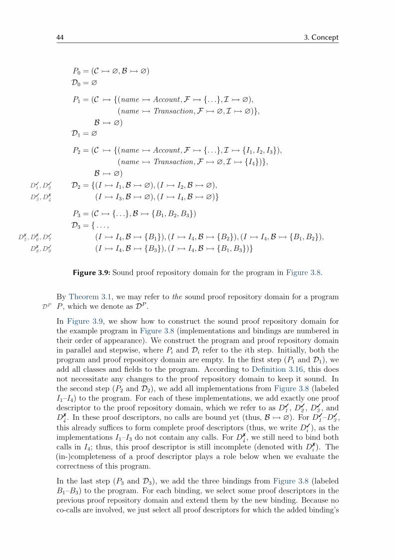
44 3. Concept
P0 = (C � ∅,B� ∅)
D0 = ∅
P1 = (C � {(name � Account ,F � {. . .}, I � ∅),
(name � Transaction,F � ∅, I � ∅)},B � ∅)
D1 = ∅
P2 = (C � {(name � Account ,F � {. . .}, I � {I1, I2, I3}),(name � Transaction,F � ∅, I � {I4})},
B � ∅)
D2 = {D31 , D
32 (I � I1,B� ∅), (I � I2,B� ∅),
D33 , D
74 (I � I3,B� ∅), (I � I4,B� ∅)}
P3 = (C � {. . .},B� {B1, B2, B3})D3 = { . . . ,
D75 , D
76 , D
37 (I � I4,B� {B1}), (I � I4,B� {B2}), (I � I4,B� {B1, B2}),
D78 , D
39 (I � I4,B� {B3}), (I � I4,B� {B1, B3})}
Figure 3.9: Sound proof repository domain for the program in Figure 3.8.
By Theorem 3.1, we may refer to the sound proof repository domain for a programP , which we denote asDP DP .
In Figure 3.9, we show how to construct the sound proof repository domain forthe example program in Figure 3.8 (implementations and bindings are numbered intheir order of appearance). We construct the program and proof repository domainin parallel and stepwise, where Pi and Di refer to the ith step. Initially, both theprogram and proof repository domain are empty. In the first step (P1 and D1), weadd all classes and fields to the program. According to Definition 3.16, this doesnot necessitate any changes to the proof repository domain to keep it sound. Inthe second step (P2 and D2), we add all implementations from Figure 3.8 (labeledI1–I4) to the program. For each of these implementations, we add exactly one proofdescriptor to the proof repository domain, which we refer to as D3
1 , D32 , D3
3 , andD7
4 . In these proof descriptors, no calls are bound yet (thus, B� ∅). For D31 –D3
3 ,
this already suffices to form complete proof descriptors (thus, we write D3i ), as the
implementations I1–I3 do not contain any calls. For D74 , we still need to bind both
calls in I4; thus, this proof descriptor is still incomplete (denoted with D7i ). The
(in-)completeness of a proof descriptor plays a role below when we evaluate thecorrectness of this program.
In the last step (P3 and D3), we add the three bindings from Figure 3.8 (labeledB1–B3) to the program. For each binding, we select some proof descriptors in theprevious proof repository domain and extend them by the new binding. Because noco-calls are involved, we just select all proof descriptors for which the added binding’s
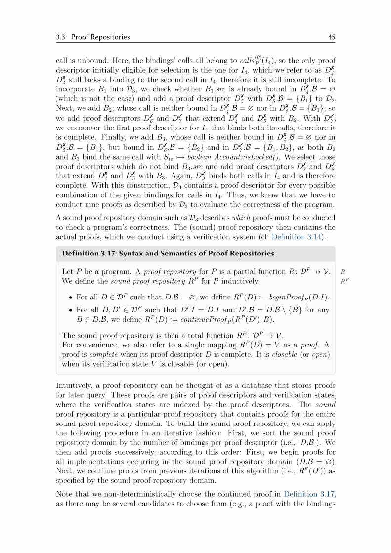
3.3. Proof Repositories 45
call is unbound. Here, the bindings’ calls all belong to calls(0)P (I4), so the only proof
descriptor initially eligible for selection is the one for I4, which we refer to as D74 .
D74 still lacks a binding to the second call in I4, therefore it is still incomplete. To
incorporate B1 into D3, we check whether B1.src is already bound in D74 .B = ∅
(which is not the case) and add a proof descriptor D75 with D7
5 .B = {B1} to D3.Next, we add B2, whose call is neither bound in D7
4 .B = ∅ nor in D75 .B = {B1}, so
we add proof descriptors D76 and D3
7 that extend D74 and D7
5 with B2. With D37 ,
we encounter the first proof descriptor for I4 that binds both its calls, therefore itis complete. Finally, we add B3, whose call is neither bound in D7
4 .B = ∅ nor in
D75 .B = {B1}, but bound in D7
6 .B = {B2} and in D37 .B = {B1, B2}, as both B2
and B3 bind the same call with Sto � boolean Account::isLocked(). We select thoseproof descriptors which do not bind B3.src and add proof descriptors D7
8 and D39
that extend D74 and D7
5 with B3. Again, D39 binds both calls in I4 and is therefore
complete. With this construction, D3 contains a proof descriptor for every possiblecombination of the given bindings for calls in I4. Thus, we know that we have toconduct nine proofs as described by D3 to evaluate the correctness of the program.
A sound proof repository domain such as D3 describes which proofs must be conductedto check a program’s correctness. The (sound) proof repository then contains theactual proofs, which we conduct using a verification system (cf. Definition 3.14).
Definition 3.17: Syntax and Semantics of Proof Repositories
Let P be a program. A proof repository for P is a partial function RR : DP 7→ V .We define the sound proof repository RPRP for P inductively.
• For all D ∈ DP such that D.B = ∅, we define RP(D) := beginProofP(D.I).
• For all D,D′ ∈ DP such that D′.I = D.I and D′.B = D.B \ {B} for anyB ∈ D.B, we define RP(D) := continueProofP(RP(D′), B).
The sound proof repository is then a total function RP : DP → V .For convenience, we also refer to a single mapping RP(D) = V as a proof. Aproof is complete when its proof descriptor D is complete. It is closable (or open)when its verification state V is closable (or open).
Intuitively, a proof repository can be thought of as a database that stores proofsfor later query. These proofs are pairs of proof descriptors and verification states,where the verification states are indexed by the proof descriptors. The soundproof repository is a particular proof repository that contains proofs for the entiresound proof repository domain. To build the sound proof repository, we can applythe following procedure in an iterative fashion: First, we sort the sound proofrepository domain by the number of bindings per proof descriptor (i.e., |D.B|). Wethen add proofs successively, according to this order: First, we begin proofs forall implementations occurring in the sound proof repository domain (D.B = ∅).Next, we continue proofs from previous iterations of this algorithm (i.e., RP(D′)) asspecified by the sound proof repository domain.
Note that we non-deterministically choose the continued proof in Definition 3.17,as there may be several candidates to choose from (e.g., a proof with the bindings

46 3. Concept
{B1, B2} can be constructed from the bindings {B1} as well as {B2}). Nonetheless,we can refer to the sound proof repository, as we show in the following theorem.
Theorem 3.2
For any program, the sound proof repository is well-defined up to equivalence ofverification states.
Proof. By (3.8), continueProof (or cP for short) commutes up to equivalence ofverification states. We can also visualize this as a commutative diagram [Mac Lane,1978], where all paths from one point to another arrive at equivalent results:
V V1
V2 V ′
cP (·,B1)
cP (·,B2) cP (·,B2)
cP (·,B1)
That is, we can choose freely whether we want to construct V ′ by binding B2
in V1 or B1 in V2, as both arrive at equivalent verification states. By appendingthis diagram to itself, we can construct larger diagrams that still commute. Inparticular, this shows that when constructing a verification state V ′ that encodessome bindings, we can continue any verification state V that encodes all bindingsbut one. Thus, no matter how we choose B ∈ D.B in the induction step ofDefinition 3.17, we arrive at equivalent verification states.In addition, there is, by construction, always at least one possible choice of B ∈ D.B(cf. Definition 3.16). Together, both arguments show well-definedness.
With Theorem 3.2, we justify our mentions of the sound proof repository above.In particular, the sound proof repository RP for a program P is also unique up toequivalence of verification states. This is fine for our purposes, because our usage ofverification states cannot distinguish equivalent verification states. Note that, whileall non-deterministic choices made in Definition 3.17 lead to equivalent sound proofrepositories, some may be more sensible than others in terms of total verificationeffort, depending on the concrete verification system.
In Figure 3.10b, we visualize in a DAG how to construct the sound proof repositoryfor the example program in Figure 3.8 according to the procedure described above.We show the final sound proof repository in Figure 3.10a. To begin with, we sortall nine proof descriptors Di by their number of bindings Di.B, which yields threegroups of proof descriptors: Those without bindings (D3
1 –D33 and D7
4 ), those withone binding (D7
5 .B = {B1}, D76 .B = {B2}, and D7
8 .B = {B3}) and those with twobindings (D3
7 .B = {B1, B2} and D39 .B = {B1, B3}). To process the first group, we
call beginProof on the implementations I1–I4, which yields four verification states.Some of these verification states are already closable (denoted as V 3
i ); that is,the proven implementations already satisfy their contracts without considering anybindings. In particular, this happens for the implementations I1–I3, which do notcontain any calls. Because I4 contains two calls, its verification state V 7
4 is notclosable until both calls are bound.

3.3. Proof Repositories 47
RP : DP → V
D31 7→ V 3
1 D76 7→ V 7
6
D32 7→ V 3
2 D37 7→ V 3
7
D33 7→ V 3
3 D78 7→ V 7
8
D74 7→ V 7
4 D39 7→ V 3
9
D75 7→ V 7
5
(a) Sound proof repository
V 75 V 3
7
V 32 V 7
6 V 39
V 74 V 7
8
V 31
cP (·,B2)
cP (·,B3 )
V 33
cP(·,B1)
cP(·,B1)
cP(·,B2)
cP (·,B3)
cP(·,B1)
(b) Visualization as a DAG
Figure 3.10: Sound proof repository RP for the program P in Figure 3.8 with thesound proof repository domain DP from Figure 3.9.
In the next iteration, we conduct proofs for the proof descriptors D75 , D7
6 andD7
8 . To do so, we choose a binding in D75 .B, D7
6 .B and D78 .B (i.e., B1, B2, and
B3, respectively) and call continueProof on the verification state from the previousiteration whose descriptor does not contain the chosen binding. That is, we callcontinueProof on V 7
4 for D75 , D7
6 and D78 , binding B1, B2, and B3, respectively. None
of the resulting verification states V 75 , V 7
6 , and V 78 are closable because there still
remains one unbound call in each of them. In the last iteration, we bind theseremaining calls according to the same principle. The only difference is that wehave several possibilities to conduct the proofs for the proof descriptors D3
7 and
D39 : For D3
7 , we can either choose to continue the proof from V 75 by binding B2
or, alternatively, from V 76 by binding B1. That is, there are two paths from V 7
4
to V 37 , which form a commuting square (drawn in red) as shown in the proof for
Theorem 3.2. According to the commuting square (i.e., the confluence property (3.8)),the verification system guarantees that both paths will yield equivalent verificationstates. In this case, both will arrive at a closable verification state V 3
7 , as all callsare now bound and the implementation I4 actually satisfies its contract under thebindings B1 and B2. Analogously, there are two ways to compute the verificationstate V 3
9 for D39 (via V 7
5 and V 78 , respectively). Again, these paths form a commuting
square (drawn in blue); therefore we can choose whichever path we like. In total,there are four ways this sound proof repository can be constructed (i.e., by combiningeach red path with each blue path). However, by our reasoning above, they mayonly differ in the internal details of their verification states and will all have theform of the sound proof repository shown in Figure 3.10a. In fact, every sound proofrepository construction corresponds to one spanning tree of the DAG visualizationin Figure 3.10b [Kruskal, 1956].
To construct this sound proof repository, we conducted nine proofs. The first fourproofs (for the proof descriptors D3
1 –D33 and D7
4 ) can be expected to be the mostcomplex proofs, as they verify (nearly) all properties specified in the implementations’contracts. Assuming a verification system that implements proper partial proofs,the other five proofs (for the proof descriptors D7
5 , D76 , D3
7 , D78 , and D3
9 ) can beexpected to require less verification effort, as they only continue existing proofs (i.e.,they apply the method contract rule for some bound call). The proof reuse gained

48 3. Concept
with proof repositories is now as follows: Suppose we would add another binding forthe call to boolean Account::isLocked() to the example program in Figure 3.8. Thiswould extend the sound proof repository with two new proofs, one that continuesV 74 and one that continues said proof or V 7
5 , which requires low verification effort ina suitable verification system. That is, extending a program with new bindings isgenerally cheap with proof repositories, which we leverage for CSPLs in Section 3.5.
By now, we are able to construct sound proof repositories for arbitrary programs.Finally, we describe how to query such a repository to characterize the correctness ofa program.
Definition 3.18: Semantics of Programs
We define the semantics of a program P as
JP K JP K :=∧
D∈DP ,unboundCallsP (D)=∅JRP(D)K.
P is then correct if and only if |= JP K (i.e., all complete proofs are also closable).
Thus, the sound proof repository for a correct program can actually contain openproofs; however, such proofs are necessarily incomplete because they have unboundcalls. Put differently, a program P is incorrect if there is at least one complete, butopen proof in RP . For instance, we can evaluate the correctness of the exampleprogram in Figure 3.8 as follows: Regarding its sound proof repository in Figure 3.10a,we check whether all complete proof descriptors (D3
i ) also map to closable verificationstates (V 3
i ). This is the case, therefore the example program is correct according toDefinition 3.18. Note that this querying phase is computationally cheap, as it doesnot require any verification effort.
We justify our definition of program correctness with the following theorem, whichrelates Definition 3.18 to the satisfaction of contracts. We adapt this theorem fromBubel et al. [2016, Theorem 2], omitting its proof.
Theorem 3.3
In a correct program without any co-calls, all implementations satisfy theircontracts for any combination of proof-completing bindings.
Thus, the semantics for the correctness of programs intuitively correspond to thesatisfaction of contracts. In particular, we can easily trace back a fault in an incorrectprogram to some complete, but open proof, which allows us to infer the faultyimplementation and combination of bindings. In Section 3.4, we describe how toleverage this property to debug faults in CbC trees.
To conclude this section, we briefly analyze the computational complexity of proofrepositories as introduced by Bubel et al. In particular, we aim to derive a closedformula that allows us to determine the number of conducted proofs beforehand.Such a formula may give us some insight as to when proof repositories are most orleast efficient. In this brief analysis, we focus on the special case of programs without
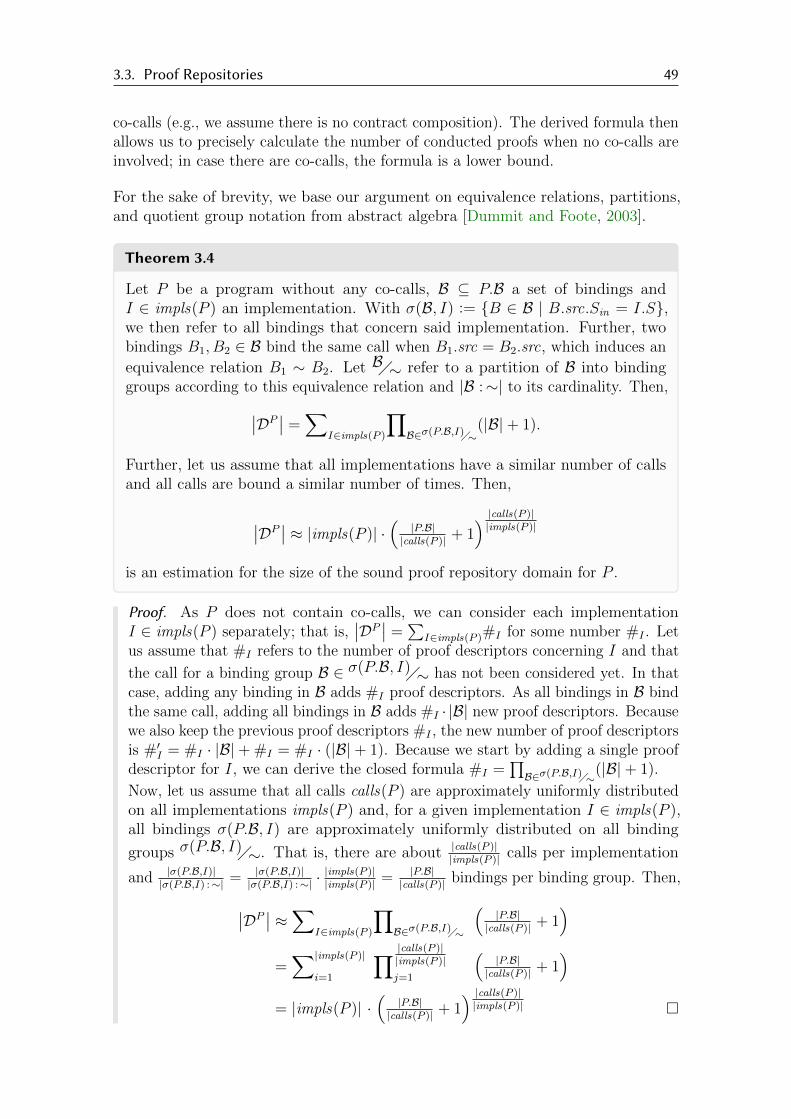
3.3. Proof Repositories 49
co-calls (e.g., we assume there is no contract composition). The derived formula thenallows us to precisely calculate the number of conducted proofs when no co-calls areinvolved; in case there are co-calls, the formula is a lower bound.
For the sake of brevity, we base our argument on equivalence relations, partitions,and quotient group notation from abstract algebra [Dummit and Foote, 2003].
Theorem 3.4
Let P be a program without any co-calls, B ⊆ P.B a set of bindings andI ∈ impls(P ) an implementation. With σ(B, I) := {B ∈ B | B.src.Sin = I.S},we then refer to all bindings that concern said implementation. Further, twobindings B1, B2 ∈ B bind the same call when B1.src = B2.src, which induces an
equivalence relation B1 ∼ B2. Let B�∼ refer to a partition of B into bindinggroups according to this equivalence relation and |B :∼| to its cardinality. Then,∣∣DP ∣∣ =
∑I∈impls(P )
∏B∈σ(P.B,I)�∼
(|B|+ 1).
Further, let us assume that all implementations have a similar number of callsand all calls are bound a similar number of times. Then,
∣∣DP ∣∣ ≈ |impls(P )| ·(|P.B||calls(P )| + 1
) |calls(P )||impls(P )|
is an estimation for the size of the sound proof repository domain for P .
Proof. As P does not contain co-calls, we can consider each implementationI ∈ impls(P ) separately; that is,
∣∣DP ∣∣ =∑
I∈impls(P )#I for some number #I . Letus assume that #I refers to the number of proof descriptors concerning I and that
the call for a binding group B ∈ σ(P.B, I)�∼ has not been considered yet. In thatcase, adding any binding in B adds #I proof descriptors. As all bindings in B bindthe same call, adding all bindings in B adds #I · |B| new proof descriptors. Becausewe also keep the previous proof descriptors #I , the new number of proof descriptorsis #′I = #I · |B|+ #I = #I · (|B|+ 1). Because we start by adding a single proofdescriptor for I, we can derive the closed formula #I =
∏B∈σ(P.B,I)�∼
(|B|+ 1).
Now, let us assume that all calls calls(P ) are approximately uniformly distributedon all implementations impls(P ) and, for a given implementation I ∈ impls(P ),all bindings σ(P.B, I) are approximately uniformly distributed on all binding
groups σ(P.B, I)�∼. That is, there are about |calls(P )||impls(P )| calls per implementation
and |σ(P.B,I)||σ(P.B,I) :∼| = |σ(P.B,I)|
|σ(P.B,I) :∼| ·|impls(P )||impls(P )| = |P.B|
|calls(P )| bindings per binding group. Then,
∣∣DP ∣∣ ≈∑I∈impls(P )
∏B∈σ(P.B,I)�∼
(|P.B||calls(P )| + 1
)=∑|impls(P )|
i=1
∏ |calls(P )||impls(P )|j=1
(|P.B||calls(P )| + 1
)= |impls(P )| ·
(|P.B||calls(P )| + 1
) |calls(P )||impls(P )| �
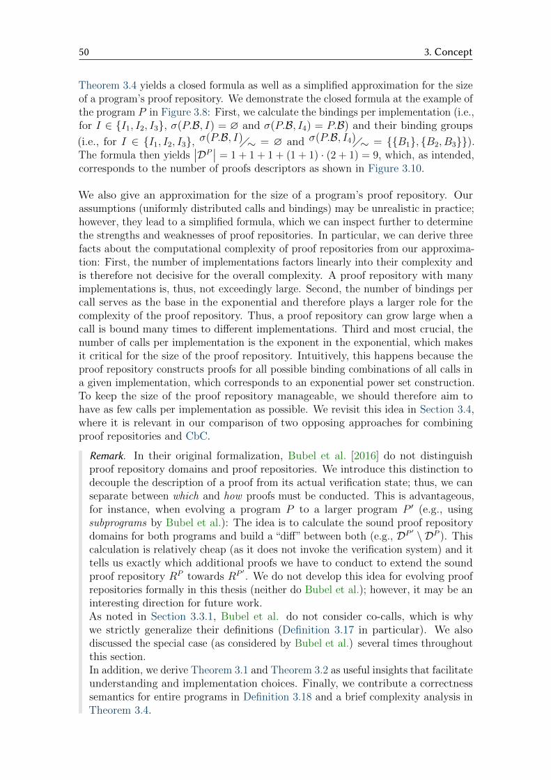
50 3. Concept
Theorem 3.4 yields a closed formula as well as a simplified approximation for the sizeof a program’s proof repository. We demonstrate the closed formula at the example ofthe program P in Figure 3.8: First, we calculate the bindings per implementation (i.e.,for I ∈ {I1, I2, I3}, σ(P.B, I) = ∅ and σ(P.B, I4) = P.B) and their binding groups
(i.e., for I ∈ {I1, I2, I3}, σ(P.B, I)�∼ = ∅ and σ(P.B, I4)�∼ = {{B1}, {B2, B3}}).The formula then yields
∣∣DP ∣∣ = 1 + 1 + 1 + (1 + 1) · (2 + 1) = 9, which, as intended,corresponds to the number of proofs descriptors as shown in Figure 3.10.
We also give an approximation for the size of a program’s proof repository. Ourassumptions (uniformly distributed calls and bindings) may be unrealistic in practice;however, they lead to a simplified formula, which we can inspect further to determinethe strengths and weaknesses of proof repositories. In particular, we can derive threefacts about the computational complexity of proof repositories from our approxima-tion: First, the number of implementations factors linearly into their complexity andis therefore not decisive for the overall complexity. A proof repository with manyimplementations is, thus, not exceedingly large. Second, the number of bindings percall serves as the base in the exponential and therefore plays a larger role for thecomplexity of the proof repository. Thus, a proof repository can grow large when acall is bound many times to different implementations. Third and most crucial, thenumber of calls per implementation is the exponent in the exponential, which makesit critical for the size of the proof repository. Intuitively, this happens because theproof repository constructs proofs for all possible binding combinations of all calls ina given implementation, which corresponds to an exponential power set construction.To keep the size of the proof repository manageable, we should therefore aim tohave as few calls per implementation as possible. We revisit this idea in Section 3.4,where it is relevant in our comparison of two opposing approaches for combiningproof repositories and CbC.
Remark. In their original formalization, Bubel et al. [2016] do not distinguishproof repository domains and proof repositories. We introduce this distinction todecouple the description of a proof from its actual verification state; thus, we canseparate between which and how proofs must be conducted. This is advantageous,for instance, when evolving a program P to a larger program P ′ (e.g., usingsubprograms by Bubel et al.): The idea is to calculate the sound proof repositorydomains for both programs and build a “diff” between both (e.g., DP ′ \ DP ). Thiscalculation is relatively cheap (as it does not invoke the verification system) and ittells us exactly which additional proofs we have to conduct to extend the soundproof repository RP towards RP ′
. We do not develop this idea for evolving proofrepositories formally in this thesis (neither do Bubel et al.); however, it may be aninteresting direction for future work.As noted in Section 3.3.1, Bubel et al. do not consider co-calls, which is whywe strictly generalize their definitions (Definition 3.17 in particular). We alsodiscussed the special case (as considered by Bubel et al.) several times throughoutthis section.In addition, we derive Theorem 3.1 and Theorem 3.2 as useful insights that facilitateunderstanding and implementation choices. Finally, we contribute a correctnesssemantics for entire programs in Definition 3.18 and a brief complexity analysis inTheorem 3.4.

3.4. Reducing Method Semantics to Proof Repositories 51
3.4 Reducing Method Semantics to Proof RepositoriesIn Section 3.1 and Section 3.2, we formally introduced CbC and CSPLs and theircorrectness semantics. The problem with evaluating a CSPL’s correctness, however, isthat we need to derive and check a product for each configuration. This is potentiallyinefficient, as there might be exponentially many configurations in a product line.Instead of checking each configuration in isolation, we strive for a solution that checkseach method in isolation. Such a solution may leverage similarities of a given methodover all configurations in the CSPL; that is, it has potential for proof reuse. As thenumber of methods is not usually subject to a combinatorial explosion, this allows,in theory, for a much more efficient evaluation of CSPL correctness.
In Section 3.3, we described proof repositories and their potential for proof reuse bycontinuing proofs and storing them for later reference. Thus, proof repositories area suitable candidate for the solution approach outlined above. In this section andSection 3.5, we apply proofs repositories to CSPLs and, thus, develop our idea fordecreasing the verification effort for CSPLs. The first step towards this goal is todraw a connection between individual methods of a CSPL and proof repositories,which we do in this section.
Basically, our idea in this section is to transform a method in the sense of Definition 3.7into a program in the sense of Definition 3.12. We can then construct a sound proofrepository for said program, from which we may then draw conclusions about thecorrectness of the original method. In summary, we aim to reduce the correctnesssemantics of methods to the correctness semantics of programs and their sound proofrepositories.
As a first step towards transforming methods into programs, we make some supple-mentary definitions, which let us describe our reduction below more concisely.
Definition 3.19: Supplementary Transformations
Let M be a method. First, let SMt,nSMt,n := t M.S.name::n() denote a signature
with type t and name n that is scoped to M . In addition, let SMmainSMmain :=M.S.type M.S.name::main(M.S.(pi)) denote the main signature of M .Further, provided that M is complete and given a node N ∈M.T.N and its edges
{N i−→Ni} ⊆M.T.E such that M .T .H (N) ' {∗} s {∗}, let sMNsMN := s[( i)\(sMNi)]
refer to the inline statement of N (where sMN = s if there are no such edges).
In addition, let FMFM := {t M.S.name::n | t n ∈M.L ∪M.S.(pi)} ∪{M.S.type M.S.name::�}
and rMbrMb := {(S � SMmain ,
requires � bφc,ensures � bψc,assignable � bAM.T c,body � b) | Hroot(M.T ) ' {φ} ∗ {ψ}}
refer to the field and root transformation of M .

52 3. Concept
In this and the following definitions, the implementation-specific functionb·c b·c shalltranslate conditions (e.g., φ), assignable locations (e.g., ATN ), and statements (e.g.,sMN ) into the specification and implementation languages of the proof repository(i.e., JML and Java). In particular, b·c must
• translate loops with while and weave (in-)variants of repetitions into thegenerated code (i.e., with the JML keywords loop_invariant and decreases),
• ensure the side condition for exclusive cases in a selection (i.e., by prependingan if statement that encodes said side condition),
• and take into account the return variable where necessary (i.e., by appendingreturn �;).
We explain this and the following definitions at the example of the method MList Insert
from the CSPL in Figure 3.4, which inserts an integer into a list. We use the CbCtree for this method as it is given in Figure 3.1 (but, still, replacing A′ with �). Inparticular, we include the faulty guard definition (χG := i < len(�) instead of thecorrect χG := i < len(A)). Our goal is then to detect this fault with our reduction,and trace it to its origin (i.e., the guard definition), if possible.
First, Definition 3.19 introduces the following new notations and transformations:
• SMt,n generates a signature scoped to M . Below, we use this to create signaturesthat correspond to a given node N in a method’s CbC tree. For example, theroot node of MList Insert .T has the signature SMList Insert
void, 1© = void List Insert:: 1©().
• Similarly, SMmain generates a signature named main that represents M as a whole(e.g., SMList Insert
main = int[] List Insert::main(int[] A, int x)). Below, we use thismain signature to bind calls from one method to another.
• With sMN , we can create a single, large statement for M that is suitable formethod inlining. For example, by recursively substituting all abstract statementsstarting at the root node of MList Insert .T , we arrive at the inline statement
sMList Insert1© = i, �, �[len(�)− 1] := 0, new int[len(A) + 1], x
[χM ] do [χI , eV ] χG → �[i], i := A[i], i+ 1 od,
which we use in Section 3.4.1 for a lightweight transformation into programs.
• The field transformation of M transforms local variables, parameters, and thereturn variable of M into a set of corresponding fields in a program.
• The root transformation of M creates an implementation with the main signatureof M . This is necessary so that we can call and bind to M from other methods.The contract of the created implementation is based on the root node’s Hoaretriple, while we supply its body as b. We also translate the assignable locationsof M.T to a matching assignable clause.
• Finally, b·c translates FOL and GCL expressions into JML and Java, which ofteninvolves only minor substitutions (e.g., ∧ and ∨ by && and ||). Below, we discussexamples that further clarify the three requirements in Definition 3.19 regardingrepetitions, selections, and return variables.
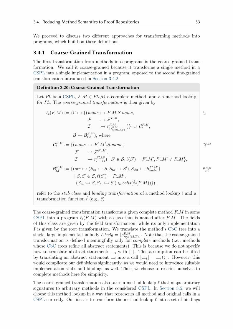
3.4. Reducing Method Semantics to Proof Repositories 53
We proceed to discuss two different approaches for transforming methods intoprograms, which build on these definitions.
3.4.1 Coarse-Grained TransformationThe first transformation from methods into programs is the coarse-grained trans-formation. We call it coarse-grained because it transforms a single method in aCSPL into a single implementation in a program, opposed to the second fine-grainedtransformation introduced in Section 3.4.2.
Definition 3.20: Coarse-Grained Transformation
Let PL be a CSPL, F M ∈ PL.M a complete method, and ` a method lookupfor PL. The coarse-grained transformation is then given by
c`c`(F M) := (C � {(name � F M.S.name,
F � FF M ,
I � rF MbsF M
root(M.T )c)} ∪ C
F M` ,
B� BF M`,c ), where
CF M`CF M` := {(name � F ′M ′.S.name,
F � FF ′ M ′,
I � rF′ M ′
();) | S ′ ∈ S, `(S ′) = F ′M ′, F ′M ′ 6= F M},
BF M`,t
BF M`,t
:= {(src � (Sin � S, Sto � S ′), Sdst � SF′ M ′
main )
| S, S ′ ∈ S, `(S ′) = F ′M ′,
(Sin � S, Sto � S ′) ∈ calls (t`(F M))}).
refer to the stub class and binding transformation of a method lookup ` and atransformation function t (e.g., c).
The coarse-grained transformation transforms a given complete method F M in someCSPL into a program c`(F M) with a class that is named after F M . The fieldsof this class are given by the field transformation, while its only implementationI is given by the root transformation. We translate the method’s CbC tree into asingle, large implementation body I.body = bsF M
root(M.T )c. Note that the coarse-grainedtransformation is defined meaningfully only for complete methods (i.e., methodswhose CbC trees refine all abstract statements). This is because we do not specifyhow to translate abstract statements i with b·c. This assumption can be liftedby translating an abstract statement i into a call b ic = i();. However, thiswould complicate our definitions significantly, as we would need to introduce suitableimplementation stubs and bindings as well. Thus, we choose to restrict ourselves tocomplete methods here for simplicity.
The coarse-grained transformation also takes a method lookup ` that maps arbitrarysignatures to arbitrary methods in the considered CSPL. In Section 3.5, we willchoose this method lookup in a way that represents all method and original calls in aCSPL correctly. Our idea is to transform the method lookup ` into a set of bindings

54 3. Concept
(C � {(name � List Insert,
F � {int[] List Insert::A, int List Insert::x,
int List Insert::i, int[] List Insert::�},I � {(S �Imain int[] List Insert::main(int[] A, int x),
requires � A.length > 0,
ensures � �.length == A.length + 1 && app(�, x)
&& appAll(�, 0, A.length,A),
assignable � i, �, �[�.length - 1], �[i],body � i = 0, � = new int[A.length + 1],
�[�.length - 1] = x;
/*@ loop_invariant �.length == A.length+1
@ && app(�, x) && 0<=i && i<=A.length
@ && appAll(�, 0, i, A);
@ decreases A.length - i;
@ assignable �[i], i; @*/
while (i < �.length)�[i] = A[i], i = i + 1;
return �;)})},B � ∅)
Figure 3.11: Coarse-grained transformation of MList Insert into a program.
that binds all calls in the transformed implementation I to the main signatures ofmethods in the CSPL as given by `. To this end, we employ the stub class and bindingtransformations: The binding transformation unwraps all mappings `(S ′) = F ′M ′
in the given method lookup and transforms them into bindings with all calls to S ′ assource and the main signature of F ′M ′ as destination. The stub class transformationthen contains stub classes with a single implementation whose only purpose is toserve as “dummy” destinations for these bindings (with a call (); as body, whichwe never bind at all). In Section 3.5, we replace these stub classes with the actualtransformed methods to describe a transformation from whole CSPLs into programs.
We give two examples to describe the coarse-grained transformation in detail, onethat disregards the stub class and binding transformations and one that includesboth. In Figure 3.11, we show the coarse-grained transformation of the completemethod MList Insert in Figure 3.4. For the method lookup, we choose the emptymethod lookup `∅ (i.e., `∅(S) is undefined for all S ∈ S), because this particularmethod does not contain any calls we could bind. Thus, CMList Insert
`∅= BMList Insert
`∅,c= ∅
in this example. The transformed program c`∅(MList Insert) therefore consists of asingle class List Insert and no bindings. We encode the parameters A and x, theloop variable i, and the return variable � as fields in this class. Equivalently, wecould also encode the local variable i as an actual stack-allocated local variablein the main implementation—we use fields instead, which ensures compatibilitywith the second transformation introduced in Section 3.4.2. We then inline the

3.4. Reducing Method Semantics to Proof Repositories 55
actual CbC tree in its entirety in a single main implementation Imain added bythe root transformation, which we may then verify in one piece. To support theverification system in verifying the repetition (which we translate as a while loop),we must supply its invariant and variant using the JML keywords loop_invariant
and decreases, respectively. Note that we do not allow the JML keyword \result inHoare triples, as pre- and postconditions are plain FOL formulas. Instead, we alwaysutilize the return variable �, which is equivalent. Again, this ensures compatibilitywith the second transformation, which we explain in Section 3.4.2. However, we stillreturn � in the body of Imain with return �;, simply to ensure that Imain is type-safe.
As introduced in Definition 3.20, the coarse-grained transformation merely constructsa program c`(F M) for a given complete method F M and method lookup `. However,this is only the first step: To evaluate the correctness of the transformed programc`(F M), we still need to construct its sound proof repository Rc`(F M), which iswhere the actual verification effort lies. For the example shown in Figure 3.11, thisis rather simple: Because the transformed program P := c`∅(MList Insert) has a singleimplementation and no bindings, the associated sound proof repository domainwill always comprise a single proof descriptor (in line with Definition 3.16); thus,DP = {D3}, where D3 = (I � Imain ,B� ∅). We may then construct the soundproof repository for P with any verification system that conforms to Definition 3.14,which yields
RP : DP → VD3 7→ V 7.
RP comprises a single proof for Imain , which is complete (D3) because Imain does notcontain any calls. However, this proof is also open (i.e., its proof descriptor D3 mapsto an open verification state V 7) because the loop condition i < �.length in Imain isfaulty, which is a direct consequence of the faulty guard definition χG := i < len(�)in the original CbC tree. We can now evaluate the transformed program’s correctness(according to Definition 3.18) and come to the conclusion that this program is, indeed,incorrect. However, we are not able to pinpoint the exact location of the fault in theprogram (and, thus, in the original CbC tree), which is due to the coarse granularityof the transformation. Instead, we may investigate the verification state V 7 manually(e.g., inspect proof nodes with KeY) or try to reduce the program to a minimumexample that still exhibits the fault; however, both approaches are error-prone andrequire expertise in the verification system. We address this problem with our secondfine-grained transformation introduced in Section 3.4.2 and discuss it further inSection 3.4.3. However, despite this issue, the coarse-grained transformation is alightweight tool to assert that a complete method, of which we suspect that it is`-correct, is indeed `-correct.
Next, we discuss another example of how to apply the coarse-grained transformation.Note that within Figure 3.11, we show how to transform a complete method thatdoes not contain any original or method calls. We show the more general case inFigure 3.12 with the coarse-grained transformation of MSet Insert from the CSPLin Figure 3.4. This method also inserts an integer into a data structure; however,it does so on sets (i.e., unordered lists with duplicate elimination) or ordered sets,depending on the configuration of the CSPL. Thus, the implementation and contract
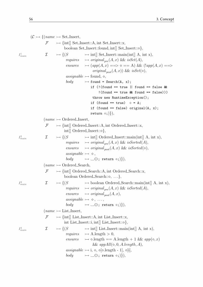
56 3. Concept
(C � {(name � Set Insert,
F � {int[] Set Insert::A, int Set Insert::x,
boolean Set Insert::found, int[] Set Insert::�},I � {(S �I1main int[] Set Insert::main(int[] A, int x),
requires � originalpre(A, x) && isSet(A),
ensures � (app(A, x) ==> � == A) && (!app(A, x) ==>
originalpost(A, x)) && isSet(�),assignable � found, �,body � found = Search(A, x);
if (!(found == true || found == false &&
!(found == true && found == false)))
throw new RuntimeException();
if (found == true) � = A;
if (found == false) original(A, x);
return �;)}),(name � Ordered Insert,
F � {int[] Ordered Insert::A, int Ordered Insert::x,
int[] Ordered Insert::�},I � {(S �I2main int[] Ordered Insert::main(int[] A, int x),
requires � originalpre(A, x) && isSorted(A),
ensures � originalpost(A, x) && isSorted(�),assignable � � ,body � (); return �;)}),
(name � Ordered Search,
F � {int[] Ordered Search::A, int Ordered Search::x,
boolean Ordered Search::�, . . .},I � {(S �I3main boolean Ordered Search::main(int[] A, int x),
requires � originalpre(A, x) && isSorted(A),
ensures � originalpost(A, x),
assignable � � , . . . ,body � (); return �;)}),
(name � List Insert,
F � {int[] List Insert::A, int List Insert::x,
int List Insert::i, int[] List Insert::�},I � {(S �I4main int[] List Insert::main(int[] A, int x),
requires � A.length > 0,
ensures � �.length == A.length + 1 && app(�, x)
&& appAll(�, 0, A.length,A),
assignable � i, �, �[�.length - 1], �[i],body � (); return �;)}),

3.4. Reducing Method Semantics to Proof Repositories 57
(name � List Search,
F � {int[] List Search::A, int List Search::x,
boolean List Search::�, . . .},I � {(S � I5mainboolean List Search::main(int[] A, int x),
requires � len(A) > 0,
ensures � � == true <==> app(A, x),
assignable � � , . . . ,body � (); return �;)})},
B � {(src � (Sin � B1int[] Set Insert::main(int[] A, int x),
Sto � int[] Set Insert::original(int[] A, int x)),Sdst � int[] Ordered Insert::main(int[] A, int x)),
(src � (Sin � B2int[] Set Insert::main(int[] A, int x),
Sto � boolean Set Insert::Search(int[] A)),Sdst � boolean Ordered Search::main(int[] A, int x)),
(src � (Sin � B3int[] Ordered Insert::main(int[] A, int x),
Sto � int[] Ordered Insert::original(int[] A, int x)),Sdst � int[] List Insert::main(int[] A, int x)),
(src � (Sin � B4boolean Ordered Search::main(int[] A, int x),
Sto � boolean Ordered Search::original(int[] A, int x)),Sdst � boolean List Search::main(int[] A, int x))})
Figure 3.12: Coarse-grained transformation of MSet Insert into a program.
of this method depend on its original method, which we specify using the (up to nowdisregarded) method lookup. In the example in Figure 3.12, we utilize a methodlookup ` as given by
` : S 7→ PL.Mint[] Set Insert::original(int[] A, int x) 7→MOrdered Insert
boolean Set Insert::Search(int[] A, int x) 7→MOrdered Search
int[] Ordered Insert::original(int[] A, int x) 7→MList Insert
boolean Ordered Search::original(int[] A, int x) 7→MList Search .
This method lookup is part of the method lookup visualized in Figure 3.7d. Thus,the transformed program c`(MSet Insert) represents the particular variant of MSet Insert
that is derived in the configuration {List,Ordered, Set} (i.e., insertion into orderedsets). By verifying the transformed program, we can therefore show the `-correctnessof this particular variant of MSet Insert (we describe how to check all variants of amethod in Section 3.5, here we focus on single variants).
First, we transform the CbC tree of MSet Insert into a single class Set Insert with onemain implementation I1main in a similar fashion as described above for MList Insert . Inthe body of I1main , we show how to translate a selection in a CbC tree into Java code:That is, we translate each case into a single if statement with the translated case’s

58 3. Concept
guard condition (e.g., if (found == true) � = A;). The order of these if statements
does not matter due to the side condition φ→∨n
i=1χGi for exclusive selection cases(cf. Definition 3.10). To guarantee this side condition, we prepend another if
statement that signals an exception should the side condition not be satisfied (i.e.,when found is neither true or false or found is true and false at the same time,which is both impossible as expected). The verification system should then handlethe thrown exception as an abnormal termination (e.g., with a normal_behavior
specification case in JML) and fail to close the respective proof. Thus, we canguarantee that exactly one of the guard conditions (e.g., either found = true orfound = false) is satisfied.
Different from the coarse-grained transformation for MList Insert shown in Figure 3.11,MSet Insert contains original and method calls. More precisely, its contract calls itsoriginal precondition with originalpre and its original postcondition with originalpost .Further, the CbC tree of MSet Insert calls Search and original . It now depends onthe method lookup ` how we process these calls. With our particular choice of` in mind, we want to interpret the original calls as calls to MOrdered Insert andthe Search calls as a call to MOrdered Search , just as depicted in Figure 3.7d. Tothis end, we include two bindings for these calls with the appropriate signaturesusing the binding transformation: First (B1), we bind the original calls (with thesignature int[] Set Insert::original(int[] A, int x)) in the implementation Set Insert(or int[] Set Insert::main(int[] A, int x)) to Ordered Insert (or int[] Ordered Insert::main(int[] A, int x)). This binding covers all three original calls in MSet Insert (i.e.,originalpre , originalpost , and original). Second (B2), we bind the Search methodcall (with the signature boolean Set Insert::Search(int[] A)) to Ordered Search (orboolean Ordered Search::main(int[] A, int x)).
For these bindings to be meaningful according to Figure 3.8, we must also supplyimplementations for the binding destinations. We do so using the stub class transfor-mation by adding two stub classes Ordered Insert and Ordered Search, both witha single implementation (I2main and I3main) specifying the contracts of MOrdered Insert
and MOrdered Search , respectively, as given in Figure 3.4. As we are not interestedin the implementations (and the `-correctness) of these methods, we only providethem with a “dummy” body (in the form of a call ();). This is fine because toverify MSet Insert , applying the method contract rule only requires the contracts ofall called methods, not their implementations. We never bind these “dummy” calls,therefore these stub classes cannot affect the overall correctness of c`(MSet Insert) (asonly complete proofs contribute to program correctness).
We are not done yet, however: Both the contract of MOrdered Insert and MOrdered Search
in turn invoke their original contract with originalpre and originalpost . This is aninstance of contract composition as explained in Section 3.2; that is, the contract ofMSet Insert not only depends on the contracts of MOrdered Insert and MOrdered Search , buton their original contracts as well, in a recursive fashion. We can address this with theother two mappings in `, which we have not discussed yet: One maps the original callin MOrdered Insert to MList Insert and the other maps the original call in MOrdered Search
to MList Search . Similarly to above, we transform both mappings into bindings (B3 andB4) to int[] List Insert::main(int[] A, int x) and boolean List Search::main(int[] A,int x), respectively. For these bindings to be meaningful, we also add stub classes for

3.4. Reducing Method Semantics to Proof Repositories 59
Ordered Insert(7,7)
(7,7)
List Insert(7,7)
(7,7) (7,7) (7,7) (3,3)
(7,7) (7,7)
Set Insert(7,7)
(7,7) (7,7)
cP (·,B3)
Ordered Search(7,7)
(7,7)cP (·,B4)
List Search(7,7)
cP (·,B3)
cP (·,B2 )
cP (·,B2) cP (·,B4)
cP(·,B
3)
cP (·,B4)
cP(·,B
3)
cP(·,B1)
cP (·,B2) cP (·,B4)
cP(·,B
1)
cP(·,B
1)
Figure 3.13: Sound proof repository for the coarse-grained transformation in Fig-ure 3.12.
MList Insert and MList Search with “dummy” implementations (I4main and I5main). (Notethat the stub class for MList Insert is, save for its implementation’s body, identicalto the class in the coarse-grained transformation c`∅(MList Insert) from Figure 3.11,which we leverage in Section 3.5 to generalize our reduction to entire CSPLs.) Bothof these stub classes, in turn, do not contain any more original calls in their contracts,so the resulting program shown in Figure 3.12 binds every available call to someimplementation.
Note that, in our explanation, we took an iterative point of view (i.e., starting witha single class, then adding two bindings and stub classes, then adding bindings andstub classes again). Definition 3.20, however, allows us to calculate a coarse-grainedtransformation c`(F M) in only two steps: First, we calculate the single class namedafter F M and the stub class transformation of `, then we calculate the bindingtransformation on the resulting program, which binds all available calls accordingto `. As we demonstrated above, this calculation also takes contract composition(which correspond to the extended calls of F M) into account.
With the transformation to a program P := c`(MSet Insert) done, we again considerthe sound proof repository RP for P . In Figure 3.13, we visualize said sound proofrepository in a fashion similar to our previous DAG visualization in Figure 3.10b.On the far left, we show the five initial proofs in RP of the form RP((I � . . . ,B 7→∅)) = V , whose nodes we label with the class of the concerned implementation.All these proofs are incomplete and open (denoted as (7,7)) because they containunbound calls; in particular, the proof for Set Insert is incomplete because the callsto original and Search are not bound yet. By adding the bindings B1–B4, a gridof commuting squares emerges, in which we label a node with (7,7) if its proof isincomplete and open (or with (3,3) if its proof is complete and closable). Thestructure of this grid can be derived analogously to Figure 3.10b, which is why weomit a detailed discussion. Note, however, that none of the intermediate proofs is
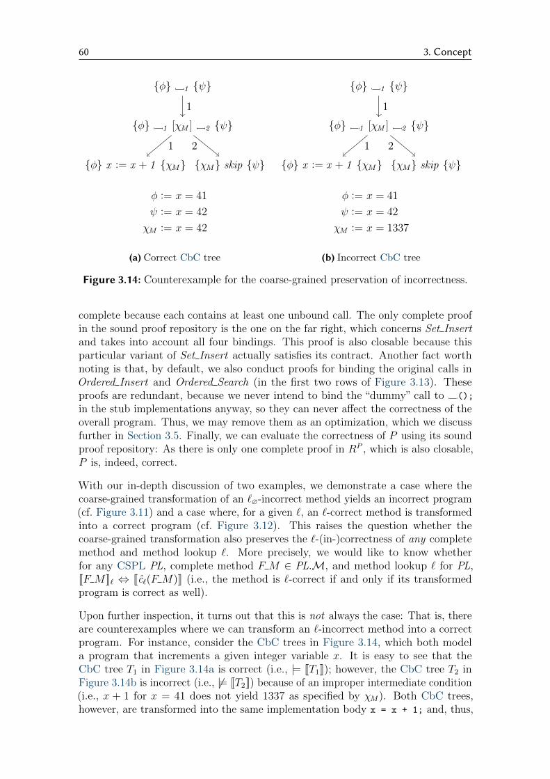
60 3. Concept
{φ} 1 {ψ}
{φ} 1 [χM ] 2 {ψ}
{φ} x := x + 1 {χM} {χM} skip {ψ}
1
1 2
φ := x = 41
ψ := x = 42
χM := x = 42
(a) Correct CbC tree
{φ} 1 {ψ}
{φ} 1 [χM ] 2 {ψ}
{φ} x := x + 1 {χM} {χM} skip {ψ}
1
1 2
φ := x = 41
ψ := x = 42
χM := x = 1337
(b) Incorrect CbC tree
Figure 3.14: Counterexample for the coarse-grained preservation of incorrectness.
complete because each contains at least one unbound call. The only complete proofin the sound proof repository is the one on the far right, which concerns Set Insertand takes into account all four bindings. This proof is also closable because thisparticular variant of Set Insert actually satisfies its contract. Another fact worthnoting is that, by default, we also conduct proofs for binding the original calls inOrdered Insert and Ordered Search (in the first two rows of Figure 3.13). Theseproofs are redundant, because we never intend to bind the “dummy” call to ();
in the stub implementations anyway, so they can never affect the correctness of theoverall program. Thus, we may remove them as an optimization, which we discussfurther in Section 3.5. Finally, we can evaluate the correctness of P using its soundproof repository: As there is only one complete proof in RP , which is also closable,P is, indeed, correct.
With our in-depth discussion of two examples, we demonstrate a case where thecoarse-grained transformation of an `∅-incorrect method yields an incorrect program(cf. Figure 3.11) and a case where, for a given `, an `-correct method is transformedinto a correct program (cf. Figure 3.12). This raises the question whether thecoarse-grained transformation also preserves the `-(in-)correctness of any completemethod and method lookup `. More precisely, we would like to know whetherfor any CSPL PL, complete method F M ∈ PL.M, and method lookup ` for PL,JF MK` ⇔ Jc`(F M)K (i.e., the method is `-correct if and only if its transformedprogram is correct as well).
Upon further inspection, it turns out that this is not always the case: That is, thereare counterexamples where we can transform an `-incorrect method into a correctprogram. For instance, consider the CbC trees in Figure 3.14, which both modela program that increments a given integer variable x. It is easy to see that theCbC tree T1 in Figure 3.14a is correct (i.e., |= JT1K); however, the CbC tree T2 inFigure 3.14b is incorrect (i.e., 6|= JT2K) because of an improper intermediate condition(i.e., x + 1 for x = 41 does not yield 1337 as specified by χM). Both CbC trees,however, are transformed into the same implementation body x = x + 1; and, thus,

3.4. Reducing Method Semantics to Proof Repositories 61
their transformed programs P1 = P2 are identical for any method lookup `. Supposethe coarse-grained transformation would preserve the `-incorrectness of completemethods, then we could conclude JT1K ⇔ JP1K ⇔ JP2K ⇔ JT2K, which contradicts6|= JT2K. The underlying reason why the coarse-grained transformation cannot preservethe `-incorrectness of all complete methods is that all intermediate conditions in aCbC tree are lost in the translation by b·c. This is because a verification systemsuch as KeY does not directly allow for the translation of intermediate conditions.Thus, the coarse-grained transformation is not injective on CbC trees that are onlydistinguished by intermediate conditions, and can therefore not detect faults inintermediate conditions at all.
There is one more scenario where the coarse-grained transformation fails to detectfaults, which involves the method lookup `. Suppose the CbC tree for MSet Insert inFigure 3.4 contained only the selection case with the guard condition found = true.In that case, MSet Insert would be `-incorrect for any method lookup ` (as the side
condition φ→∨n
i=1χGi would be violated); however, its coarse-grained transformationc`∅(MSet Insert) would be correct for the empty method lookup `∅ (as its sound proofrepository would only comprise incomplete proofs). The reason why c cannot detectthis fault is its coarse granularity: Because we do not clearly separate each sidecondition from Definition 3.10 in the coarse-grained transformation, all side conditionsof a CbC tree are verified in one piece. A single unbound call, however, causes therespective proofs to be incomplete, so they cannot contribute to the transformedprogram’s correctness (cf. Definition 3.18). Put differently, the program semanticsare not injective on CbC trees that contain unbound calls, and can therefore notdetect faults when a method lookup does not bind all calls.
However, despite these issues, we can actually infer a weaker form of the propositionstated above: That is, the coarse-grained transformation may not be able to detect allfaults in a complete method, but all detected faults are actual faults. Put differently,it cannot preserve `-incorrectness, but `-correctness of complete methods.
Theorem 3.5
For any CSPL PL, complete method F M ∈ PL.M, and method lookup ` for PL,JF MK` ⇒ Jc`(F M)K.
The proof for Theorem 3.5 largely depends on a suitable translation b·c from FOLconditions and GCL statements into the specification and implementation languagesof the proof repository. Intuitively, this translation is mostly straightforward forJML and Java (as seen in Figure 3.11 and Figure 3.12); formally, however, it israther technical, which makes it difficult to fully develop this proof, therefore we omitit. Structurally, a full proof would also be similar to the proofs we present for thefine-grained transformation in Section 3.4.2 (i.e., it requires a structural inductionon the method lookup `).
The consequence of Theorem 3.5 is that, instead of asserting the `-correctness ofa complete method using the semantics presented in Definition 3.10, we can alsoequivalently assert the correctness of its transformed program. This is the key topotential savings in verification effort when we describe a transformation from entire

62 3. Concept
CSPLs into programs in Section 3.5. However, the above-described flaw in the coarse-grained transformation still remains: It is not a proper reduction of the correctnesssemantics of methods to the correctness semantics of programs, as it cannot reliablydetect all faults in methods. Nonetheless, the coarse-grained transformation is afirst approach to combine CbC with proof repositories that also has its own justifiedapplication scenarios, which we further discuss in Section 3.4.3.
3.4.2 Fine-Grained TransformationAs a counterpart to the lightweight coarse-grained transformation and its drawbacks,we define a second transformation from methods into programs: the fine-grainedtransformation. This transformation takes a different approach; namely, it transformsnodes in a method’s CbC tree into many separate, small implementations.
Definition 3.21: Fine-Grained Transformation
Let PL be a CSPL, F M ∈ PL.M a method, and ` a method lookup for PL. Thefine-grained transformation is then given by
f` f`(F M) := (C � {(name � F M.S.name,
F � FF M ,
I � rF M(); ∪
{(S � SF Mvoid,N ,
requires � bφc,ensures � bψc,assignable � bAM.T
N c,body � bsc)| N ∈M.T.N ,M .T .H (N) ' {φ} s {ψ},s is not refinable}∪ IF M
sel ∪ IF Minit ∪ IF M
use )} ∪ CF M` ,
B� BF M`,f
), where
IF Msel IF Msel := {(S � SF M
boolean,N sel , requires � bφc, ensures � \result ,
assignable � \nothing , body � return b∨n
i=1χGic;)
| N ∈M.T.N ,M .T .H (N) ' {φ} if (χGi → i)ni=1 fi {∗}},
IF Minit IF Minit := {(S � SF M
void,N init , requires � bφc, ensures � bχIc,assignable � \nothing , body � ;)
| N ∈M.T.N ,M .T .H (N) ' {φ} do [χI , eV ] χG → 1 od {∗}}, and
IF Muse IF Muse := {(S � SF M
boolean,N use , requires � bχIc, ensures � !\result ==> bψc,assignable � \nothing , body � return bχGc;)
| N ∈M.T.N ,M .T .H (N) ' {∗} do [χI , eV ] χG → 1 od {ψ}}
refer to the side condition transformations of F M .

3.4. Reducing Method Semantics to Proof Repositories 63
Similar to the coarse-grained transformation, the fine-grained transformation trans-forms a given method F M and method lookup ` in some CSPL into a programf`(F M) with a class named after F M , whose fields are again given by the fieldtransformation. However, in contrast to the coarse-grained transformation, thefine-grained transformation is applicable to any method (incomplete ones as well)and can therefore also be used to assess the `-correctness of a partially developedmethod. Another difference is that the main implementation added by the roottransformation rM (); contains only a “dummy” call to ;, as this implementation isonly necessary to interface with other methods in Section 3.5.
We add the actual Hoare triples of the method as separate implementations to theprogram, with one implementation per node N ∈ F M.T.N whenever the statementin the node’s Hoare triple is not refinable. That is, we add an implementation forevery node that has a skip statement, an assignment, or a method call (in a completemethod, these correspond directly to the leaves of its CbC tree). For each addedimplementation, we assign it the contract of its Hoare triple (translated into JMLas bφc and bψc) and, as implementation body, we use the Hoare triple’s statement(translated into Java as bsc). To cover abstract statements and compositions, we donot need to add any implementations, as both kinds of statements do not imposeany side conditions. (The only condition that a composition 1 [M ] 2 imposes,namely that their child edges must share an intermediate condition M , is alreadyguaranteed on a syntactical level by Definition 3.2.)
Finally, to cover the side conditions of selections and repetitions, we add moreimplementations that arise from the three side condition transformations IF M
sel , IF Minit ,
and IF Muse given in Definition 3.21: First, for each selection in the method’s CbC
tree, IF Msel adds an implementation that encodes the side condition φ →
∨n
i=1χGiof correct selections from Definition 3.10. This implementation assumes bφc in itsrequires clause and ensures that \result yields true; that is, the JML expression
b∨n
i=1χGic is satisfied (this translation can be performed with the JML operators
&&, ||, and ! according to the definition of∨
given in Section 2.2). We could alsotry to encode said expression directly in the ensures condition; however, as thetranslated guards bχGic are Java expressions, they should only be used in the bodyof an implementation.
Then, for each repetition in the method’s CbC tree, IF Minit and IF M
use encode the sideconditions φ→ χI and χI ∧ ¬χG → ψ from Definition 3.10 in a similar fashion: Theimplementations added by IF M
init require bφc and ensure bχIc, which encodes theinitial satisfaction of all invariants. Finally, the implementations added by IF M
use
require bχIc and ensure !\result ==> bψc, where the truth of \result is given by theexpression bχGc. Again, bχGc is a Java expression and, thus, only usable within animplementation body, so we refer to it in the ensures clause with the \result keyword.Defined this way, the implementations added by IF M
use encode the correct usage of allinvariants. Note that we do not need to explicitly address loop termination here, as itis already encoded in the Hoare triples of the CbC tree per Definition 3.2. Altogether,the implementations added by the side condition transformations should cover allside conditions for `-correct methods (cf. Definition 3.10); below, we show that thisis actually the case.

64 3. Concept
Note that we do not need to transform a repetition such as do [χI , eV ] χG →1 od into an actual while loop with a JML contract (i.e., /*@ loop_invariant
bχIc; decreases beV c; */ while (bχGc) 1();) as we did for the coarse-grainedtransformation in Figure 3.11. This is because we already split up the proof obligationsfor repetitions at the transformation level: That is, the implementations added byIF Minit and IF M
use encode the initial invariant satisfaction and its correct usage. Wefurther guarantee the invariant’s preservation with the implementation that is addedfor the Hoare triple refining the abstract statement 1, if any. Together, these threeproof obligations (and their corresponding implementations) are almost equivalentto supplying a single implementation with a while loop. However, separating theseproof obligations facilitates subsequent debugging and evolution of a method (whichwe discuss in Section 3.4.3).
In addition, this approach also avoids a subtle correctness issue regarding incom-plete methods: Consider an incomplete CbC tree with a repetition Hoare triple{φ} do [χI , eV ] χG → 1 od {ψ}, where the abstract statement 1 is unrefined.Further, imagine that a modified fine-grained transformation f ′ added a single imple-mentation I for a while loop, instead of splitting up the three proof obligations asoutlined above. Because 1 is not refined, the proof for I in a sound proof repositorywill be incomplete and, thus, not contribute to the correctness of the f ′-transformedprogram (cf. Definition 3.18). Suppose further that φ→ χI is not valid and thereforethe CbC tree is necessarily incorrect (because φ→ χI is a necessary side condition forrepetitions). However, as the proof for I does not contribute to program correctness,the f ′-transformed program may be correct nonetheless (provided that the remainderof the CbC tree is correct). In summary, we have described a scenario where a CbCtree is not correct, but its f ′-transformed program is, which would severely restrict ourability to infer the (in-)correctness of CbC trees from their f ′-transformed programs.(This is also similar to the scenario in which the coarse-grained transformation cannotpreserve incorrectness, as we discussed in Section 3.4.1.)
It is easy, however, to fix this problem by splitting up the proof obligations andadding the implementations resulting from the side condition transformations IF M
init
and IF Muse , as we do in our unmodified definition of f . These implementations do not
contain any calls and, thus, are necessarily complete and will always contribute toprogram correctness. In the case sketched above where φ→ χI is not valid, the prooffor the implementation added by IF M
init will then be complete, but open, and thereforethe program will be incorrect as well; thus, preserving the correctness semantics ofmethods and avoiding the issue altogether. A similar line of reasoning also applies toa selection such as if (χGi → i)
ni=1 fi, which we do not need to transform into an
actual if statement as shown in Figure 3.12. Instead, one proof obligation per case(i.e., an implementation added for the Hoare triple refining the abstract statement
i, if any) and the implementation added by IF Msel suffice. Again, this facilitates
later evolution of the method and avoids the issue regarding incomplete methodsoutlined above.
To conclude our discussion of Definition 3.21, the fine-grained transformation utilizesexactly the same mechanism for incorporating a given method lookup ` as the coarse-grained transformation. That is, we use to transform ` into a set of bindings thatbinds all calls in the transformed program to methods’ main signatures as given by

3.4. Reducing Method Semantics to Proof Repositories 65
`, and we add stub classes for all these main signatures with CF M` . Intuitively, we
may further be tempted to reflect the edges (i.e., refinements between Hoare triples)in the method’s CbC tree as bindings in the transformed program. However, this isnot necessary: The conformance of Hoare triples (e.g., the requirement that childedges of a composition must share an intermediate condition) is already ensured ona syntactical level by Definition 3.2. Further, the correctness of all side conditions inDefinition 3.10 is already covered by all of the implementations we discussed above.Thus, we need no more bindings than those mandated by BF M
`,f.
In Figure 3.15, we exemplify the fine-grained transformation using the methodMList Insert from Figure 3.4. For the method lookup, we again choose the emptymethod lookup `∅, as MList Insert does not contain any bindable calls. Thus, similar tothe coarse-grained transformation, the transformed program f`∅(MList Insert) consistsof a single class List Insert and no stub classes or bindings (i.e., CMList Insert
`∅=
BMList Insert
`∅,f= ∅). However, we now add several small implementations, each of
which encodes a Hoare triple or a side condition. All of these implementationsshare access to the fields, which are given by the field transformation. In particular,all implementations can access the shared return variable �, which would not bepossible if we used the \result keyword instead (as it is scoped only to a singleimplementation).
We now discuss the implementations in Figure 3.15 in more detail. First, we add amain implementation Imain using the root transformation, which acts as an interfaceto other methods. The purpose of Imain is only to provide the contract of MList Insert ,as MList Insert itself does not have to be verified and should not contribute to thecorrectness of the transformed program. Similar to the stub class transformation,we enforce this by inserting a call (); into Imain .body , which we will never bind.The proof for Imain in the sound proof repository will then necessarily be incompleteand not contribute to program correctness (cf. Definition 3.18). Moving on, we addan implementation for every node in the CbC tree MList Insert .T with an unrefinablestatement. That is, we add implementations I 3© and I 5© for nodes 3© and 5©, whichare assignments and therefore straightforward to transform. Note that the assignablelocations derived from both assignments are propagated towards the root of the CbCtree. In the transformed program, these locations are reflected in the assignableclauses of the implementations, which may then be used by the verification systemto support proof attempts.
Note that we do not directly transform the composition in node 2© and the repetitionin node 4©. By not transforming the composition in node 2©, we do not lose anyinformation, as the implementations I 3© and I 5© already encode its correctness. Wehave already explained above why it is not necessary to transform the repetition innode 4© into an implementation of its own. Instead, we split node 4© into three proofobligations, which are encoded as three implementations: First, I 5© encodes that therepetition’s invariant is preserved and the variant decreased. Second and third, weadd two implementations using the side condition transformations IF M
init and IF Muse :
That is, I 4© init is responsible for ensuring that the invariant in node 4© is initiallysatisfied (i.e., it follows from the ensures clause of I 3©). Finally, I 3© use encodes thatthe invariant in node 4© is correctly used (i.e., it implies the ensures clause of Imain).

66 3. Concept
(C � {(name � List Insert,
F � {int[] List Insert::A, int List Insert::x,int List Insert::i, int[] List Insert::�},
I � {(S �Imain int[] List Insert::main(int[] A, int x),requires � A.length > 0,ensures � �.length == A.length + 1 && app(�, x)
&& appAll(�, 0, A.length,A),
assignable � i, �, �[�.length - 1], �[i],body � (); return �;),
(S �I 3© void List Insert:: 3©(),requires � A.length > 0,ensures � �.length==A.length+1 && app(�, x) && i==0,assignable � i, �, �[�.length - 1],body � i = 0, � = new int[A.length + 1],
�[�.length - 1] = x;),
(S �I 4© init void List Insert:: 4© init(),requires � �.length==A.length+1 && app(�, x) && i==0,ensures � �.length == A.length + 1 && app(�, x)
&& 0 <= i && i <= A.length&& appAll(�, 0, i, A),
assignable � \nothing ,body � ;),
(S �I 4© use boolean List Insert:: 4© use(),requires � �.length == A.length + 1 && app(�, x)
&& 0 <= i && i <= A.length&& appAll(�, 0, i, A),
ensures � !\result ==> (�.length == A.length + 1&& app(�, x) && appAll(�, 0, A.length,A)),
assignable � \nothing ,body � return i < �.length;),
(S �I 5© void List Insert:: 5©(),requires � �.length == A.length + 1 && app(�, x)
&& 0 <= i && i <= A.length&& appAll(�, 0, i, A) && i < �.length,
ensures � �.length == A.length + 1 && app(�, x)&& 0 <= i && i <= A.length&& appAll(�, 0, i, A) && 0 <= A.length - i&& A.length - i < \old(A.length− i),
assignable � i, �[i],body � �[i] = A[i], i = i + 1;)})},
B � ∅)
Figure 3.15: Fine-grained transformation of MList Insert into a program.

3.4. Reducing Method Semantics to Proof Repositories 67
As we have transformed the method MList Insert into a program P := f`∅(MList Insert),we can now construct its sound proof repository to evaluate the method’s `∅-correctness, just like we did for the coarse-grained transformation. The computationcan again be done with any verification system that conforms to Definition 3.14 andyields
RP : DP → V(I � Imain ,B� ∅)7 7→ V 7
1
(I � I 3©,B� ∅)3 7→ V 32
(I � I 4© init ,B� ∅)3 7→ V 33
(I � I 4© use ,B� ∅)3 7→ V 34
(I � I 5©,B� ∅)3 7→ V 75 .
This sound proof repository consists of five proofs, each one corresponding to asingle implementation in P . First, the proof for Imain is open (denoted with an openverification state V 7
1 ), because the implementation’s code does not satisfy its contract(it only contains a “dummy” call, after all). However, because this call is unbound inthe proof (as B� ∅), the proof is incomplete and does not affect the correctness ofthe program. Thus, this implementation is effectively unimportant with regard tocorrectness; however, it exposes the method’s contract to other methods, which weneed in Section 3.5 to transform entire CSPLs into programs. The next three proofsin the proof repository (belonging to the implementations I 3©, I 4© init , and I 4© use)are all complete because their implementations do not contain any calls. As requiredby Definition 3.18, they are also closable. However, the last proof, which belongs toI 5©, is complete as its implementation contains no calls, but open. Because there is acomplete, but open proof in its sound proof repository, the program P is incorrect asexpected.
The reason why the implementation I 5© does not satisfy its contract is, just as forthe coarse-grained transformation, the faulty guard definition χG := i < len(�) in theoriginal CbC tree. Although we still cannot exactly tell the exact cause of the faultjust from looking at the sound proof repository, we can at least infer that it must bedue to the repetition (and not, for example, the assignment in node 2©). Because theproofs for the two side conditions of the repetition are closable, we can conclude thatthe fault occurs because the invariant is not preserved properly. Note that, in contrastto the coarse-grained transformation, we were able to pin down the location of thefault to some degree without investigating any verification states manually. Thus, thefine-grained transformation nicely complements the coarse-grained transformationwith its debugging capabilities.
Above, we also discussed the coarse-grained transformation of MSet Insert , which isgiven by c`(MSet Insert) for a defined ` (cf. Figure 3.12). The fine-grained trans-formation of MSet Insert , given by f`(MSet Insert), then merely combines the ideasfrom previously discussed examples: That is, we simply transform the CbC treeMSet Insert .T into a number of small implementations as demonstrated in Figure 3.15,while we incorporate the stub class and binding transformations in exactly thesame way shown in Figure 3.12. Because this is rather straightforward, we omit a
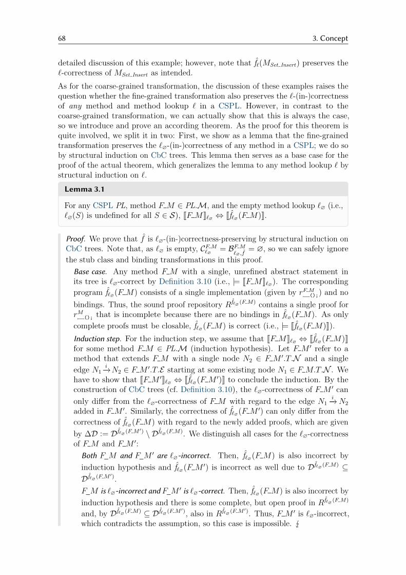
68 3. Concept
detailed discussion of this example; however, note that f`(MSet Insert) preserves the`-correctness of MSet Insert as intended.
As for the coarse-grained transformation, the discussion of these examples raises thequestion whether the fine-grained transformation also preserves the `-(in-)correctnessof any method and method lookup ` in a CSPL. However, in contrast to thecoarse-grained transformation, we can actually show that this is always the case,so we introduce and prove an according theorem. As the proof for this theorem isquite involved, we split it in two: First, we show as a lemma that the fine-grainedtransformation preserves the `∅-(in-)correctness of any method in a CSPL; we do soby structural induction on CbC trees. This lemma then serves as a base case for theproof of the actual theorem, which generalizes the lemma to any method lookup ` bystructural induction on `.
Lemma 3.1
For any CSPL PL, method F M ∈ PL.M, and the empty method lookup `∅ (i.e.,`∅(S) is undefined for all S ∈ S), JF MK`∅ ⇔ Jf`∅(F M)K.
Proof. We prove that f is `∅-(in-)correctness-preserving by structural induction onCbC trees. Note that, as `∅ is empty, CF M
`∅ = BF M`∅,f
= ∅, so we can safely ignore
the stub class and binding transformations in this proof.
Base case. Any method F M with a single, unrefined abstract statement inits tree is `∅-correct by Definition 3.10 (i.e., |= JF MK`∅). The corresponding
program f`∅(F M) consists of a single implementation (given by rF M();) and no
bindings. Thus, the sound proof repository Rf`∅ (F M) contains a single proof forrM (); that is incomplete because there are no bindings in f`∅(F M). As only
complete proofs must be closable, f`∅(F M) is correct (i.e., |= Jf`∅(F M)K).Induction step. For the induction step, we assume that JF MK`∅ ⇔ Jf`∅(F M)Kfor some method F M ∈ PL.M (induction hypothesis). Let F M ′ refer to amethod that extends F M with a single node N2 ∈ F M ′.T.N and a single
edge N1i−→N2 ∈ F M ′.T.E starting at some existing node N1 ∈ F M.T.N . We
have to show that JF M ′K`∅ ⇔ Jf`∅(F M ′)K to conclude the induction. By theconstruction of CbC trees (cf. Definition 3.10), the `∅-correctness of F M ′ can
only differ from the `∅-correctness of F M with regard to the edge N1i−→N2
added in F M ′. Similarly, the correctness of f`∅(F M ′) can only differ from the
correctness of f`∅(F M) with regard to the newly added proofs, which are given
by ∆D := Df`∅ (F M ′) \ Df`∅ (F M). We distinguish all cases for the `∅-correctnessof F M and F M ′:
Both F_M and F_M ′ are `∅-incorrect. Then, f`∅(F M) is also incorrect by
induction hypothesis and f`∅(F M ′) is incorrect as well due to Df`∅ (F M) ⊆Df`∅ (F M ′).
F_M is `∅-incorrect and F_M ′ is `∅-correct. Then, f`∅(F M) is also incorrect by
induction hypothesis and there is some complete, but open proof in Rf`∅ (F M)
and, by Df`∅ (F M) ⊆ Df`∅ (F M ′), also in Rf`∅ (F M ′). Thus, F M ′ is `∅-incorrect,which contradicts the assumption, so this case is impossible.

3.4. Reducing Method Semantics to Proof Repositories 69
F_M is `∅-correct and F_M ′ is `∅-incorrect. Then, f`∅(F M) is also correct byinduction hypothesis, so we have to find a newly added proof described by∆D that is complete, but open. By construction (see above), adding the edge
N1i−→N2 rendered F M ′ `∅-incorrect. As the added node N2 is a leaf node
by construction and has no child edges, JN2j−→ ∗KF M ′
`∅ in Definition 3.10 isvacuously true. Thus, some side condition must have been violated. Note that|= `∅
F M ′
φ,ψ because `∅ is empty; thus, no original calls are involved (i.e., φF M ′
`∅ =
φ and ψF M ′
`∅ = ψ). To investigate further, we distinguish all possibilities forthe kind of the statement s in F M ′.T .H (N2) = {∗} s {∗}:
Skip statement, assignment, selection, and repetition. In these cases, we addnew implementations to f`∅(F M), which do not contain any calls and whoseproofs are therefore complete. Some side condition must have been violated(e.g., φ 6⇒ ψ for skip statements), which reflects in the contract of someadded implementation I ′ (assuming a proper translation function b·c). Thus,
there is a D3 ∈ ∆D with D3 = (I � I ′,B� ∅) and R f`∅ (F M ′)(D3) = V 7I ′ .
This proof is complete, but open and, thus, f`∅(F M ′) is incorrect. Theargument for assignments, selections, and repetitions is analogous.
Method call. Because `∅ is empty, `∅(SF M (l := m(ai))) in Definition 3.10 isundefined and J{φ} l := m(ai) {ψ}KF M ′
`∅ is vacuously true. Thus, this sidecondition cannot have been violated, so this case is impossible. Abstract statement and composition. These kinds of statements do not haveany side conditions that may be violated, so these cases are impossible.
Thus, in all cases where a side condition may be violated, there is at least oneproof that is complete, but open, and f`∅(F M ′) is incorrect.
Both F_M and F_M ′ are `∅-correct. Then, f`∅(F M) is also correct by inductionhypothesis, so we have to show that all added proofs described by ∆R (ifany) are either incomplete or closable. By construction (see above), the edge
N1i−→N2 is correct and all side conditions for the statement s in M ′.T .H (N2) =
{∗} s {∗} are valid. Distinguishing all possibilities for the kind of the statements, we can make arguments that are structurally similar to the ones above, onlythis time leading to incomplete or complete, closable proofs:
Skip statement, assignment, selection, and repetition. The validity of any sidecondition of these kinds of statements will reflect in the added implementa-tion’s contract and result either in a complete, closable proof (if |= `∅
F M ′
φ,ψ )
or in an incomplete proof (if 6|= `∅F M ′
φ,ψ , in which case there is an unboundoriginal call).
Method call. The implementation added for a method call contains anunbound call, so the resulting proof is necessarily incomplete.
Abstract statement and composition. We do not add any implementations forthese kinds of statements, so we add no proofs either (∆D = ∅) and, thus,
Df`∅ (F M) = Df`∅ (F M ′).
In total, all added proofs are incomplete or closable, so f`∅(F M ′) is correct.
In all four cases, f`∅(F M ′) preserves the `∅-(in-)correctness of F M ′.
With Lemma 3.1 in place, we can show the actual theorem.
70 3. Concept
Theorem 3.6
For any CSPL PL, method F M ∈ PL.M, and method lookup ` for PL, JF MK` ⇔Jf`(F M)K.
Proof. We prove that f is `-(in-)correctness-preserving by structural induction onthe method lookup `, starting with the empty `∅, which we extend step-by-step.
Base case. In this case, we show that f preserves the `∅-(in-)correctness of amethod F M . That is, we consider F M in isolation from other methods, so wehave to show JF MK`∅ ⇔ Jf`∅(F M)K, which corresponds to Lemma 3.1.
Induction step. In this case, we show that f preserves the `-(in-)correctness of amethod F M also when F M interacts with other methods by means of bindings.Assuming that JF MK` ⇔ Jf`(F M)K for some method F M ∈ PL.M and somemethod lookup ` (induction hypothesis), we have to show that JF MK`′ ⇔Jf`′(F M)K, where `′ extends ` with a single new mapping `′(S ′) = F ′M ′ (i.e.,`′(S) = `(S) for all S 6= S ′). By the construction of CbC trees (cf. Definition 3.10),the `′-correctness of F M can only differ from the `-correctness of F M withregard to the new mapping `′(S ′) = F ′M ′ added in `′. Similarly, the correctnessof f`′(F M) can only differ from the correctness of f`(F M) with regard to
the newly added proofs, which are given by ∆D := Df`′ (F M) \ Df`(F M). Wedistinguish all cases for the `- and `′-correctness of F M :
F_M is both `- and `′-incorrect, F_M is `-incorrect and `′-correct. The argumentsare analogous to those made in the proof for Lemma 3.1.
F_M is `-correct and `′-incorrect. Then, f`(F M) is also correct by inductionhypothesis, so we have to find an added proof described by ∆D that is complete,but open. By construction (see above), adding the mapping `′(S ′) = F ′M ′
rendered F M `′-incorrect. Thus, some side condition in Definition 3.10 musthave been violated for 6|= JF MK`′ . By the definition of f , the violated sidecondition corresponds to a single implementation I in f`′(F M). To investigatefurther, we distinguish all possibilities for the kind of the statement whoseside condition was violated:
Skip statement, assignment, selection, and repetition. A side condition in Defi-nition 3.10 for these kinds of statements can only be affected by the newmapping in `′ when 6|= `F M
φ,ψ ; in that case the new mapping may “activate”
the side condition (i.e., |= `′F Mφ,ψ ) and contribute to the `′-correctness of
F M . Because |= `′F Mφ,ψ , all original calls for the violated side condition
can be looked up with `′. Because of this and by the definition of BF M`′,f
and sound proof repository domains (cf. Definition 3.16), there must bea complete proof descriptor D ∈ ∆D with D.I = I. Assuming a propertranslation function b·c, the violation of the side condition reflects in the
involved contracts; thus, the proof R f`′ (F M )(D) is complete, but open andf`′(F M) is incorrect.
Method call. An argument similar to the previous kinds of statements canbe made, the only difference being that the side condition for method callsis activated when |= `′(SF M (l := m(ai))) = F ′M ′ ∧ `′F M
φ,ψ ∧ `′F ′ M ′
φ′,ψ′ .
3.4. Reducing Method Semantics to Proof Repositories 71
Abstract statement and composition. These kinds of statements do not haveany side conditions that may be violated, so these cases are impossible.
Thus, in all cases where a side condition may be violated, there is at least oneproof that is complete, but open, and f`′(F M) is incorrect.
F_M is both `- and `′-correct. Then, f`(F M) is also correct by inductionhypothesis, so we have to show that all all added proofs described by ∆D (ifany) are either incomplete or closable. By construction (see above), addingthe mapping `′(S ′) = F ′M ′ kept F M `′-correct; in particular, all activatedside conditions (see above) are still valid. Now, let I be any implementationthat corresponds to an activated side condition. Analogous to our argumentabove, there must be a complete proof descriptor D ∈ ∆D with D.I = I.However, different from above, the validity of the side condition will reflect inthe involved contracts; thus, R f`′ (F M )(D) is closable and f`′(F M) is correct.
In all four cases, f`′(F M) preserves the `′-(in-)correctness of F M .
The significance of Theorem 3.6 is analogous to that of Theorem 3.5: Namely, itallows us to evaluate the correctness of a transformed program f`(F M) instead ofthe `-correctness of the original method F M (with potential savings in verificationeffort). In contrast to the coarse-grained transformation, however, the fine-grainedtransformation can detect all faults in a method, and is therefore a proper reductionof method correctness to program correctness.
Besides the practical implications of this theorem, it is also of theoretical interest:We have shown that a decision problem about methods (i.e., asking the question “isthe method F M `-correct?”) is many-one reducible to a decision problem aboutprograms (i.e., asking the question “is the program f`(F M) correct?”) [Post, 1944].This implies that methods are, without restrictions, embeddable into programs andthat evaluating the correctness of the former is not harder (regarding computationalcomplexity) than the latter. Omitting a proof, we can even show that f (whenimplemented appropriately) is a polynomial-time many-one reduction (with respect tothe number of calls and size of CbC trees in the CSPL). That is, f is also sufficientlyefficient in transforming complete methods into programs, which is of practicalrelevance for our implementation in Chapter 4.
3.4.3 Discussion
Above, we extensively described and explained the coarse- and fine-grained trans-formations from methods into programs. We also investigated the properties ofboth transformations with regard to the preservation of method (in-)correctness.In this section, we compare both transformations and highlight their respective(dis-)advantages for different scenarios.
In Figure 3.16, we show the key findings of our discussion. We compare the coarse-grained transformation c and the fine-grained transformation f with respect toseveral criteria regarding usability, correctness, and efficiency. Below, we discuss eachcriterion and our findings in more detail.
Applicability. Because we do not translate abstract statements in a CbC tree withb·c, c can only transform complete methods. Thus, it is (as described in this thesis)

72 3. Concept
Coarse-Grained (c) Fine-Grained (f)
Applicability Complete methods All methods
Correctness Pres. JF MK` ⇒ Jc`(F M)K JF MK` ⇔ Jf`(F M)KComplexity Polynomial-time Polynomial-timeVerification Effort Few large proofs Many small proofs
For many calls Many large proofs Many small proofsDebugging Requires inspection Up to side conditionsEvolution Requires re-verification Up to side conditions
Figure 3.16: Comparison of the coarse- and fine-grained transformations.
not suited for developing a CbC tree from scratch and then applying successiverefinements, which is the primary use case for CbC. However, with some additionalimplementation stubs and bindings, this restriction can be lifted (although omittedin this thesis). The fine-grained transformation f does not have this problem becauseit intentionally separates all nodes in a CbC tree and does not require any abstractstatements to be translated.
Correctness Preservation. Both transformations can be used to refute the `-correctnessof a method F M ; that is, if their transformed programs are incorrect, the originalmethod is `-incorrect as well. However, f can also be used to confirm the `-correctnessof F M , while c, in general, cannot. Above, we discussed two scenarios where c cannotdetect all faults: First, c cannot detect faults related to intermediate conditionsin compositions. One might, however, argue that intermediate conditions are notrelevant to the constructed CbC tree as long as the final result is correct. Thisis a matter of perspective, and how closely a developer wants to conform to theCbC methodology. Second, c may overlook faults when not all calls in a methodare bound. Note, however, that no later than when all calls are bound, c will alsodiscover such a fault. Thus, one might argue that c does detect all faults, only somein a “delayed” fashion until all calls are bound. To summarize, f avoids some subtlecorrectness issues which c does not; however, when a developer chooses to neglectthese subtleties, c is a viable alternative.
Complexity. Both transformations traverse the entire CbC tree of a method anduse the same stub class and binding transformations, therefore they have essentiallythe same computational complexity. Note that both transformations are reasonablycheap to compute even for large CSPLs, as they do not invoke the verification system.
Verification E�ort. With verification effort, we refer to how expensive it is to calculatethe sound proof repository and conduct the actual proofs with the verificationsystem. As we discussed in Section 3.3, the computational complexity (i.e., size) of aprogram’s proof repository is mostly influenced by three parameters: The number ofimplementations in the program, the number of bindings per call, and the numberof calls per implementation, which is the most crucial of the three. Regarding thenumber of implementations, c transforms a method into one class with a singlelarge implementation (besides stub classes), while f splits a method’s CbC tree intoall its side conditions and transforms each side condition into an implementation.Thus, when we only judge by the first parameter, the coarse-grained transformation

3.4. Reducing Method Semantics to Proof Repositories 73
generally constructs fewer proofs. Regarding the number of bindings per call, bothtransformations utilize the same binding transformation, so the second parameterdoes not differ between c and f at all. However, the third parameter (the numberof calls per implementation) may differ significantly between c and f : In a fine-transformed program, the number of calls per implementation is generally limitedto one (if the implementation represents a method call) plus, potentially, a chain oforiginal calls. In a coarse-transformed program, on the other hand, the number ofcalls per implementation is unlimited and completely depends on the transformedmethod. As shown in Theorem 3.4, a large number of calls per implementation bringsabout a potentially exponential number of proofs. Thus, whether c or f requires lessverification effort depends on the number of calls in the transformed method.
Besides the size of the proof repository, we must also consider the complexity of theinvolved verification states: A coarse-transformed program usually has more complexproof obligations and verification states than the small, modular implementationsin a fine-grained transformation. It is difficult to estimate and compare the totalverification effort for calculating these verification states, as this largely depends onthe utilized verification system: For example, the KeY verification system has constantoverhead for each conducted proof, so possibly, fewer large proofs (as sometimesconstructed by c) are advantageous in terms of verification effort. However, dependingon the verification system’s support for partial proofs, the continuation of proofs inthe presence of contract composition can be expensive as well, which may give f anadvantage when a CbC tree contains only few nodes with original calls. Anotheradvantage of f over c may be that the intermediate conditions in a CbC tree (whichare ignored by c) can act as “stepping stones” to aid the verification system in theverification of compositions (without intermediate conditions, the verification systemhas to “guess” them from the entire available proof context).
To summarize, the verification effort for both transformations is difficult to anticipatein advance and, thus, difficult to compare as well, as it depends on the concreteverification system and method to be transformed; we therefore revisit this discussionin our evaluation in Chapter 5. As a general rule of thumb, the coarse-grainedtransformation c tends to construct few proofs with complex verification states whenwe assume that the transformed method has only few calls (e.g., one original and onemethod call). For many calls in the transformed method, however, the number ofproofs constructed by c may grow exponentially. The fine-grained transformation f ,on the other hand, usually constructs many proofs with less complex verification states.When the transformed method has many calls, the number of proofs constructed byf grows as well, but this growth is linear.
Debugging. When we detect a fault in a transformed program (i.e., we find a complete,but open proof in the program’s sound proof repository), we are usually interested intracing it back to its origin so we can fix our original mistake. Both transformationshandle this debugging scenario differently: Because of its coarse granularity, theproofs conducted for coarse-transformed methods cover entire CbC trees, whichmakes it hard to track down a fault just by looking at the sound proof repository.Instead, we are forced to manually inspect the open verification state in question,which usually requires expertise in the verification system. This makes c less suitedfor debugging endeavors. The fine-grained transformation, on the other hand, allows

74 3. Concept
to debug up to the level of side conditions: Because each conducted proof correspondsto a single side condition in a CbC tree, the open verification state can easily betracked down to the problematic side condition. With appropriate tool support,we can then highlight the side condition’s associated Hoare triple in the CbC treeaccordingly to catch the developer’s attention. When a developer needs more detailson the detected fault, however, they again need to inspect the verification states or,alternatively, make changes until the proof in question is closable.
Evolution. When we strictly conform to the CbC methodology, we create a CbCtree by starting off with an empty CbC tree, which we refine successively (asmentioned above). Ideally, we would like to know after each refinement whetherthe resulting CbC tree (or, by extension, method or CSPL) is still correct. Thisincremental construction is one example of an evolution scenario. Fixing a mistakeafter debugging it as described above is another example for evolution. The coarse-grained transformation c is only partially suitable for the evolution of CbC treesfor two reasons: First, it is only applicable to complete methods by default, whichexcludes the incremental construction scenario. However, even for a complete method(e.g., when fixing a mistake), any change to the method’s CbC tree necessitates a re-verification of all proofs concerning the method, which redoes most of the verificationeffort.
The fine-grained transformation, on the other hand, allows for more proof reuse inboth scenarios: In the incremental construction scenario, adding a single refinementcauses some implementations and, possibly, bindings to be added to the transformedprogram’s sound proof repository (as seen in the proof for Lemma 3.1). By theincremental nature of Definition 3.17, this does not require any re-verification, sof is well-suited for this specific scenario. When we want to fix a mistake in anexisting CbC tree, we can reuse proofs by making use of the idea outlined at theend of Section 3.3 and building a “diff” between the old and corrected CbC tree’ssound proof repositories. According to this “diff”, we can then drop some proofs thatare no longer relevant for the corrected CbC tree and add new proofs as mandatedby Definition 3.16. However, this approach has its limits, too: For instance, whenwe change the contract of some Hoare triple in a CbC tree, this may affect thecontracts of other Hoare triples in turn and necessitate a larger re-verification thanintended. Similarly, when the assignable locations of a Hoare triple evolve, thischange propagates towards the root of the CbC tree (cf. Definition 3.5), which alsonecessitates re-verification. We can conclude that f is generally better-suited forevolution scenarios than c, but that it cannot completely avoid re-verification either.
Conclusion. When considering all discussed criteria, we come to the conclusion thatthe fine-grained transformation f is generally preferable over the coarse-grainedtransformation c, as it conforms more closely to the structure of CbC trees than cand therefore allows for better proof reuse in the debugging and evolution scenarios.Depending on the transformed method, the specific verification system, and thedesired accuracy of the correctness evaluation, c can, however, be a viable alternativefor already-developed methods. Nonetheless, for the reasons listed above, we focuson the fine-grained transformation in Section 3.5, where we transform entire CSPLsinto programs. Note that we can actually replace all mentions of f in Section 3.5with c (and instances of JF MK` ⇔ Jf`(F M)K with JF MK` ⇒ Jc`(F M)K) to arrive

3.4. Reducing Method Semantics to Proof Repositories 75
at a variant of the proposed transformation from CSPLs into programs that is basedon the coarse-grained transformation.
Remark. Although the coarse-grained transformation c is not as suitable for methodsand CbC trees as the fine-grained transformation f , there is a useful applicationscenario for c where f is inappropriate: Suppose we ignore CbC, methods andCSPLs for a moment and only consider methods in the sense of FOP in the PhVscenario [Thum et al., 2012b]. That is, methods can call other methods andoriginal as described in Section 3.2, but they are constructed as a whole andverified after-the-fact. In that case, a method is essentially a “black box” thatcan either satisfy its contract or not; thus, f is not applicable at all (because itis tailored to CbC trees) and c becomes a viable solution. It is thus reasonableto conclude that f is a fine choice for evaluating the correctness of CSPLs, whilec is better-suited for FOP-based SPLs that were not constructed with the CbCmethodology.
Remark. All contributions in this section are original work. The idea of transformingan entire CbC tree into a single Java method (corresponding to the coarse-grainedtransformation) has been superficially explored (but not implemented) by Watsonet al. [2016]. Similarly, the idea of transforming each side condition in a CbC treeseparately (corresponding to the fine-grained transformation) has been implementedby Runge et al. [2019a]. However, Watson et al. do not discuss method callsand Runge et al. do not operate on a method-level, both of which we discussextensively in this section.

76 3. Concept
3.5 Reducing CSPL Semantics to Proof RepositoriesIn Section 3.4, we introduced two transformations from methods into programs that(in case of the coarse-grained transformation, partially) preserve the `-(in-)correctnessof methods. We can utilize these transformations to transform entire CSPLs intoprograms. In this section, we introduce an according transformation based on thefine-grained transformation and show that it preserves the (in-)correctness of CSPLsas well. This CSPL transformation then allows us to reason about the correctness ofa given CSPL using programs and proof repositories. As proof repositories allow forproof reuse, we aim to reduce the overall verification effort for a CSPL this way.
3.5.1 CSPL TransformationOur approach to transform an entire CSPL into a program is basically to transformevery method in a given CSPL in every configuration into a program as described inSection 3.4, which we then combine into a single, large program that represents theentire CSPL and all of its methods and configurations. To this end, we describe howto combine two programs by means of a union operator.
Definition 3.22: Union of Programs
The union of two programs P1, P2 ∈ P is given by P1∪ ∪ P2 := (C � P1.C ∪P2.C,B� P1.B ∪ P2.B).We resolve a conflict in P1.C ∪ P2.C (i.e., there are classes C1 ∈ P1.C, C2 ∈ P2.Csuch that C1 6= C2, but C1.name = C2.name) as follows: If one of C1 and C2, sayC1, is a stub class (i.e., C1 ∈ CF M
` in Definition 3.20 for some ` and F M) andfor every I1 ∈ C1.I, there is some I2 ∈ C2.I such that I1 and I2 differ at most intheir bodies, we favor C2 over C1, otherwise we leave the conflict unresolved.P1 ∪ P2 may or may not be a program itself (i.e., P1 ∪ P2 /∈ P is possible),depending on whether all conflicts can be resolved as described.
Thus, the union of two programs is given by the union of their classes and bindingsin most cases. However, when both programs contain a class with the same name,we must favor one over the other so the result is again a program itself accordingto Definition 3.12 (as a program may not contain two classes with the same name).Note that our intention with this union is to combine programs created with thefine-grained transformation f . A conflict can then only arise when a stub class namedF ′M ′.S.name in one program f`(F M) coincides with the main (non-stub) class inanother program f`′(F
′M ′), in which case we favor the latter over the former.
With this notion of program union, we can calculate the CSPL transformation of agiven CSPL PL as the union of all transformed programs for all configurations andtheir respective derived methods and method lookups in PL.
Definition 3.23: CSPL Transformation
Let PL be a CSPL. The CSPL transformation is then given by
PL PL :=⋃
C∈PL.CF M∈∇PL,C
f`CPL(F M).

3.5. Reducing CSPL Semantics to Proof Repositories 77
The transformed program constructed in Definition 3.23 then fully describes allmethods in all configurations of the given CSPL. As the union of programs is notalways a program itself (cf. Definition 3.22), we proceed to show that this is actuallythe case for the CSPL transformation; that is, the main class of a transformedmethod always overrides the corresponding stub class in other transformed methods.
Lemma 3.2
For any CSPL PL, PL ∈ P (i.e., PL is a well-defined program).
Proof. Equivalently, we show for any C1, C2 ∈ PL.C, F1 M1 ∈ ∇PL,C1 , and F2 M2 ∈∇PL,C2 , that f
`C1PL
(F1 M1) ∪ f`C2PL
(F2 M2) ∈ P .
Let us assume that there is a conflict as described in Definition 3.22 that cannotbe resolved. That is, there are classes c1 ∈ f
`C1PL
(F1 M1).C, c2 ∈ f`C2PL
(F2 M2).C such
that c1 6= c2, but c1.name = c2.name.Suppose that both c1 ∈ CF1 M1
`C1PL
and c2 ∈ CF2 M2
`C2PL
, then c1 = c2 by the definition of
the stub class transformation, which contradicts c1 6= c2. Similarly, suppose that both c1 /∈ CF1 M1
`C1PL
and c2 /∈ CF2 M2
`C2PL
, then c1 = c2 by the
definition of f , which again contradicts c1 6= c2. Thus, one of c1 and c2 is a stub class, say c1 ∈ `C1
PL and c2 /∈ `C2PL. By c1.name =
c2.name and the definitions of `C1PL and f , c1.I = rF2 M2
b and rF2 M2
b′ ⊆ c2.I. Notethat both implementations only differ in their bodies b and b′. Thus, the conflictcan, in fact, be resolved, which contradicts our initial assumption.
Per Lemma 3.2, we can conceive of PL as a program and are able to evaluate itscorrectness according to Definition 3.18, which we discuss below.
We exemplify Definition 3.23 using the CSPL PL from Figure 3.4. In Figure 3.17,we visualize which methods are derived in which configurations of this CSPL. Inthis matrix, rows correspond to configurations C and columns to methods F M . Acell (C,F M) in this matrix is marked with if its method F M is derived in itsconfiguration C (and with # if it is not). Note that the correctness of PL, accordingto Definition 3.11, is then given by the `CPL-correctness of F M for each cell (C,F M)marked with , or formally:
JPLK = JList InsertK`{List}PL∧ JList SearchK
`{List}PL∧ . . . ∧ JSet InsertK
`{List,Ordered,Set}PL
However, each cell (C,F M) marked with now also corresponds to a single trans-
formed method in PL (i.e., f`CPL(F M)). For the cells marked with , we have discussedthe according coarse- and fine-grained transformations in detail in Section 3.4; thetransformed programs for the other cells can be calculated following the same princi-ple. The CSPL transformation of PL (cf. Definition 3.23), is then given by the unionof the transformed programs for each cell (C,F M) marked with , or formally:
PL = f`{List}PL
(List Insert) ∪ f`{List}PL
(List Search) ∪ . . . ∪ f`{List,Ordered,Set}PL
(Set Insert)
Note that JPLK and PL look very similar, which suggests that the correctness of theformer may be preserved by the latter. We discuss this extensively below.

78 3. Concept
ListInsert
ListSearch
OrderedInsert
OrderedSearch
OrderedSort
SetInsert
{List} # # # #
{List,Ordered} # #
{List,Set} # # #
{List,Ordered,Set} #
Figure 3.17: Matrix visualization for the semantics of the CSPL in Figure 3.4.
(C � {(name � List Insert, F � . . . , I � . . .),
(name � List Search, F � . . . , I � . . .),
(name � Ordered Insert, F � . . . , I � . . .),
(name � Ordered Search, F � . . . , I � . . .),
(name � Ordered Sort, F � . . . , I � . . .),
(name � Set Insert, F � . . . , I � . . .)},B � {(src � (Sin �B1 int[] Ordered Insert::main(int[] A, int x),
Sto � int[] Ordered Insert::original(int[] A, int x)),Sdst � int[] List Insert::main(int[] A, int x)),
(src � (Sin �B2 int[] Ordered Insert::main(int[] A, int x),
Sto � int[] Ordered Insert::Sort(int[] A)),Sdst � int[] Ordered Sort::main(int[] A)),
(src � (Sin �B3 boolean Ordered Search::main(int[] A, int x),
Sto � boolean Ordered Search::original(int[] A, int x)),Sdst � boolean List Search::main(int[] A, int x)),
(src � (Sin �B4 int[] Ordered Sort::main(int[] A),
Sto � int[] Ordered Sort::Sort(int[] A)),Sdst � int[] Ordered Sort::main(int[] A)),
(src � (Sin �B5 int[] Set Insert::main(int[] A, int x),
Sto � int[] Set Insert::original(int[] A, int x)),Sdst � int[] List Insert::main(int[] A, int x)),
(src � (Sin �B6 int[] Set Insert::main(int[] A, int x),
Sto � int[] Set Insert::original(int[] A, int x)),Sdst � int[] Ordered Insert::main(int[] A, int x)),
(src � (Sin �B7 int[] Set Insert::main(int[] A, int x),
Sto � boolean Set Insert::Search(int[] A, int x)),Sdst � boolean List Search::main(int[] A, int x)),
(src � (Sin �B8 int[] Set Insert::main(int[] A, int x),
Sto � boolean Set Insert::Search(int[] A, int x)),Sdst � boolean Ordered Search::main(int[] A, int x))})
Figure 3.18: CSPL transformation of the CSPL in Figure 3.4 into a program.

3.5. Reducing CSPL Semantics to Proof Repositories 79
First, however, we show the transformed program PL in more detail in Figure 3.18.Note that we use the coarse-grained transformation c throughout the discussion ofthis example. We do this for the sake of brevity, as the fine-grained transformationproduces more implementations and bindings than the coarse-grained transformation;the general principle, however, carries over to the fine-grained transformation. Theprogram consists of six classes, each corresponding to one method in PL (or columnin Figure 3.17). The fields and implementations of these classes are given by thecoarse-grained transformation as discussed in Section 3.4: For instance, the classList Insert corresponds to the class List Insert from c
`{List}PL
(List Insert) as shown in
Figure 3.11 (we omit the other classes for the sake of brevity). Some transformedprograms may contain stub classes (i.e., “dummy” references to other methods),which are, however, completely overridden by the main class of another transformedprogram (according to the conflict resolution in Definition 3.22). For example,the coarse-grained transformation c
`{List,Ordered,Set}PL
(Set Insert) references the methods
Ordered Insert, Ordered Search, List Insert, and List Search (as shown in Figure 3.12)
via stub classes. In PL, these classes are, however, overridden by the coarse-grainedtransformations of their respective methods (e.g., the stub class for List Insert isoverridden by its counterpart in c
`{List}PL
(List Insert) as described above). This way,
stub references are replaced by their actual implementations, and all CbC trees in PLare fully represented in PL. As for the bindings B1–B8 in PL (which model methodand original calls in PL), they arise from the union of the bindings of all transformed
programs constituting PL. For instance, all bindings occurring in the coarse-grainedtransformation in Figure 3.12 also appear in PL.B. In total, PL.B fully represents allmethod and original calls in PL; we can also observe this by revisiting Figure 3.7,which comprises eight different calls in total, each of which is bound in PL.B.
Intuitively, the transformed program PL fully represents the original CSPL PL, sowe may be tempted to claim that the correctness of PL allows us to make immediateinferences about the correctness of PL (i.e., JPLK⇔ JPLK). While this is our ultimategoal, there is one undesirable effect left to consider. To elaborate on this issue, weshow the sound proof repository for the CSPL transformation of PL in Figure 3.19.
Again, we visualize the sound proof repository RPL with a DAG in a fashion similarto Figure 3.13; in our discussion, we also consider the red nodes and edges (which
we discuss in Section 3.5.2). In fact, the sound proof repository RPL in Figure 3.19extends the sound proof repository Rc`(Set Insert) in Figure 3.13, the only differencebeing that new proofs have been added and the proof for List Insert is now complete,but open (denoted as (3,7)). This is because the class List Insert, which is a stubclass in Figure 3.13, now represents the full CbC tree of List Insert as well (asshown in Figure 3.11), and said CbC tree contains the faulty guard definition fromFigure 3.1.
Notably, the sound proof repository in Figure 3.19 contains many proofs (16 intotal) related to the method Set Insert. This is due to two reasons: First, Set Insertcontains two calls (the calls to original and Insert), and the sound proof repositoryconstructs proofs for every possible combination of bindings for these calls. (Wealready discussed this issue in the context of our comparison of c and f in Section 3.4;this is an example where c produces a single large connected component in the DAG,

80 3. Concept
Ordered Insert(7,7)
(7,7) (3,3)
(7,7)
Ordered Sort(7,7)
(3,3)
List Search(3,3)
cP (·,B1)
cP (·,B2 )
cP (·,B2)
Ordered Search(7,7)
cP(·,B
1)
(3,3)cP (·,B3)
cP (·,B4)
List Insert(3,7)
(7,7) (7,7) (7,7) (3,3)
(7,7) (7,7)
Set Insert(7,7)
(7,7) (7,7)
(7,7) (7,7) (3,7)
(7,7) (3,3)
(7,7) (3,3)
cP (·,B1)
cP (·,B8 )
cP(·,B
7 )
cP (·,B8)
cP(·,B
7 )
cP (·,B3)
cP(·,B
1)
cP (·,B3)
cP(·,B
1)
cP(·,B 6)
cP (·,B8)
cP (·,B5 )
cP (·,B7 )
cP (·,B3)
cP(·,B
6)
cP (·,B5 )
cP(·,B
6)
cP (·,B5 )
cP (·,B8)
cP (·,B7 )
cP (·,B3)
cP (·,B5)
cP (·,B6 )
cP (·,B1)
Figure 3.19: Sound proof repository for the CSPL transformation in Figure 3.18.
while f constructs several smaller connected components.) Second, there are twovariants of Set Insert, which we can see by revisiting Figure 3.7: That is, there is onevariant that inserts into an unordered set (cf. Figure 3.7c) and one that inserts intoan ordered set (cf. Figure 3.7d). Both variants require different bindings: The firstvariant binds its original and Insert calls directly to List Insert (B5) and List Search(B7), while the second variant binds to Ordered Insert (B6) and Ordered Search (B8)instead (both of which have their own original calls that must then be bound as wellwith B1 and B3). The DAG shown in Figure 3.19 unifies all proofs for both of thesevariants in a single connected component and constructs all proofs for all possiblecombinations of the involved bindings (i.e., B1, B3, and B5–B8).
However, this construction of all imaginable combinations is also the reason why the
sound proof repository RPL does not yet represent the original CSPL PL as intended.

3.5. Reducing CSPL Semantics to Proof Repositories 81
We illustrate the problem using the example from Figure 3.19: Suppose, for amoment, that the method (and transformed program of) List Insert did not containthe faulty guard definition from Figure 3.1. In that case, PL would be correct and
PL should be correct as well. However, there is a complete, but open proof in RPL forSet Insert with the bindings B5, B8, and B3; thus, judging the correctness accordingto Definition 3.18, PL is incorrect, although PL is correct. The cause of the problemappears when we examine the bindings of this proof: B5 binds the original call inSet Insert to List Insert, while B8 binds the Search call to Ordered Search. Thus,this proof attempts to show that we can insert into an unordered set by using a binarysearch, which can only be used on ordered sets. However, there is no configurationin the CSPL in which Set Insert calls both List Insert and Ordered Search; so thisproof is, in fact, not needed and even harmful, as it detects an alleged fault thatcannot occur in any configuration of the CSPL.
When we inspect the entire proof repository RPL, we find three other proofs that arealso subject to this problem; that is, they concern a combination of bindings thatdoes not occur in any configuration of the CSPL. We mark these four problematicproofs and all their edges (i.e., invocations of the verification system) with red inFigure 3.19. As all of these proofs are potentially harmful and none of them shouldcontribute to the correctness of the transformed program, we can simply removethem from the sound proof repository. This yields a new proof repository that onlyconsists of the nodes and edges in Figure 3.19 that are not colored. We refer tothe process of removing the problematic proofs as pruning and name the new proof
repository the PL-pruned proof repository (denoted as RPLPL). The PL-pruned proof
repository now properly represents the correctness of PL (i.e., JPLK⇔ JPLKPL), aswas our original intention.
3.5.2 Syntax and Semantics of Pruned Proof Repositories
In the following, we formalize our idea of pruning the sound proof repository andshow that, using the pruned proof repository, we can actually fully preserve thecorrectness of any CSPL, which generalizes our insights from the example shown inFigure 3.19. Our basic strategy for pruning is to calculate sound proof repository fora restricted sound proof repository domain, which only retains proof descriptors witha combination of bindings that occur in some configuration of the CSPL. First, wecharacterize what it means for a combination of bindings to occur in a configuration,or, more accurately, in its method lookup. To this end, we introduce the inversebinding transformation of a set of bindings.
Definition 3.24: Inverse Binding Transformation
Let PL be a CSPL and B ⊆ P.B a set of bindings in a program P .We define the inverse binding transformation B−1
PLB−1PL as a method lookup such thatfor all F M ∈ PL.M and S ∈ S, B−1PL (S) := F M if and only if B.src.Sto = Sand B.Sdst = SF M
main for some B ∈ B, otherwise B−1PL (S) is undefined.Further, a method lookup ` for PL contains another method lookup `′ for PL(denoted as `′ vv `) if and only if for any S such that `′(S) is defined, `(S) = `′(S).
82 3. Concept
We call this the inverse binding transformation because it essentially reverses thebinding transformation of a method lookup ` (cf. Definition 3.20) and also satis-fies an according cancellation law. That is, for any CSPL PL, method lookup `,transformation function t, method F M , and set of bindings B, (BF M
`,t)−1PL = ` and
B = B′ ⇔ B−1PL = B′−1PL . We make use of both of these properties in our proofsbelow. Intuitively speaking, we can use the inverse binding transformation to linkproof descriptors and their bindings (which are concepts from the proof repositoryapproach) to their respective configurations and method lookups (which are CSPLconcepts). We make this connection in the following definition, which formallyintroduces our idea of pruning potentially problematic and unnecessary proofs.
Definition 3.25: Pruned Proof Repository
Let PL be a CSPL and P a program.We define the PL-pruned proof repository domainDPPL DPPL ⊆ DP as
DPPL := {D | D ∈ DP, D.I.body 6= ();,∨C∈PL.C
F M∈∇PL,C(D.I.S.className = F M.S.name ∧ (D.B)−1PL v `CPL)}.
We then define the PL-pruned proof repository for P asRPPL RPPL := RP |DP
PL(i.e., we
restrict its sound proof repository to its PL-pruned proof repository domain).Finally, we define the semantics for P with regard to PL, namely
JP KPL JP KPL :=∧
D∈DPPL,unboundCallsP (D)=∅
JRPPL(D)K.
P is then PL-correct if and only if |= JP KPL.
In Definition 3.25, we remove certain proof descriptors from the sound proof repositorydomain DP of a program P to arrive at the PL-pruned proof repository domain DPPL.There are three cases when we remove a given proof descriptor D: First, wheneverD concerns an implementation that contains only a call ();, we can safely skipthe described proof as we never intend to bind such calls anyway. This is a sensibleoptimization, which also facilitates our proofs below. Second, we can and mustskip D if its binding combination does not occur in any configuration, or, moreprecisely, if there is no configuration C ∈ PL.C such that (D.B)−1PL v `CPL. Third,we must also skip D if none of the configurations it occurs in derives the methodF M corresponding to D.I, or, more precisely, if there is no configuration C ∈ PL.Csuch that F M ∈ ∇PL,C . After this pruning procedure, we are only left with proofdescriptors whose implementations and bindings occur in least one configuration(as derived methods and method lookups, respectively) of the given CSPL. The PL-pruned proof repository for a program is then similar to its sound proof repository,but it omits all pruned proof descriptors. Just like before, a program is PL-correct ifand only if all complete proofs in its PL-pruned proof repository are also closable.The basic insights from Section 3.3 also extend to PL-pruned proof repositories; thatis, PL-pruned proof repository domains exist and are unique (cf. Theorem 3.1) andPL-pruned proof repositories are well-defined up to equivalence of verification states
3.5. Reducing CSPL Semantics to Proof Repositories 83
(cf. Theorem 3.2), so we may utilize them in basically the same way as sound proofrepositories.
Above, we have already shown an example PL-pruned proof repository, as theuncolored nodes and edges in Figure 3.19 form the PL-pruned proof repository forthe CSPL PL from Figure 3.4. Said CSPL is then PL-incorrect (i.e., 6|= JPLKPL) if we
include the faulty guard definition from Figure 3.1 and PL-correct (i.e., |= JPLKPL)if we use the corrected CbC tree instead. Thus, we successfully fixed the problemdescribed above where the CSPL was not correct according to the original semantics(i.e., 6|= JPLK) although we used the corrected CbC tree.
As for the coarse- and fine-grained transformations in Section 3.4, the discussionof our example raises the question whether the CSPL transformation preserves the(in-)correctness of any CSPL. We already showed above by counterexample that thisis not the case for the regular program semantics using sound proof repositories (i.e.,
there are CSPLs PL such that 6|= JPLK↔ JPLK). However, we fixed the cause of theproblem with our pruning scheme; and it turns out that we can show the desiredproperty when using PL-pruned proof repositories instead (i.e., for any CSPL PL
JPLK⇔ JPLKPL). As the proof for this theorem is again quite involved, we split itinto several lemmas, which we prove separately.
First, we connect the regular program semantics used in Section 3.3 and Section 3.4to the semantics of pruned proof repositories. That is, we show that our previousinsights about the fine-grained transformation still apply when we utilize pruned proofrepositories, as none of the pruned proof descriptors contribute to the transformedprogram’s correctness.
In the following, when a CSPL PL, configuration C ∈ PL.C and method F M ∈ PL.Mare all clear from the context, we abbreviate the method’s fine-grained transformationwith 〈f〉 := f`CPL(F M) for the sake of brevity.
Lemma 3.3
For any CSPL PL, C ∈ PL.C, and F M ∈ ∇PL,C , J〈f〉K⇔ J〈f〉KPL.
Proof. By Definition 3.25, D〈f〉PL ⊆ D〈f〉, so we have to show that all pruned proofdescriptors are incomplete and therefore do not contribute to the correctness of
〈f〉. Let D ∈ D〈f〉 \ D〈f〉PL be such a proof descriptor.Suppose that D.I has the body ();. Then, D.I is a stub implementation (i.e.,it belongs to a stub class in CF M
`CPL) or a root-transformed implementation. In both
cases, we never bind the call to ();, therefore D is incomplete.Suppose now that D.I has a body different from ();. In that case, it belongsto the class named F M.S.name in 〈f〉.C. By definition, D.B ⊆ 〈f〉.B = BF M
`CPL,f,
which inverts to (D.B)−1PL v `CPL. Thus, also D /∈ D〈f〉 \ D〈f〉PL .
Next, we show that the PL-pruned proof repository domain for PL is actually thesame as the union of the PL-pruned proof repository domains for all transformedmethods in PL. In particular, the PL-pruned proof repository domain for PL does not

84 3. Concept
contain any proof descriptors that are not already in the PL-pruned proof repositorydomain for some transformed method in PL.
Intuitively, we may also say that the whole (i.e., DPLPL) is not greater than the sum of
its parts (i.e.,⋃D〈f〉PL ).
Lemma 3.4
For any CSPL PL, DPLPL =
⋃D〈f〉PL , where
⋃D〈f〉PL :=
⋃C∈PL.C,F M∈∇PL,CD
〈f〉PL .
Proof. First, we show that DPLPL ⊇
⋃D〈f〉PL . Note that for any programs P1, P2 ∈ P
with P1 ∪ P2 ∈ P, also RP1PL ⊆ RP1∪P2
PL , because P1 ∪ P2 is an extension of P1 inthe sense of Definition 3.16. Thus, for any configuration C ∈ PL.C and derived
method F M ∈ ∇PL,C , D〈f〉PL ⊆ DPLPL, and so is their union
⋃D〈f〉PL as well.
Second, we show that DPLPL ⊆
⋃D〈f〉PL . Suppose there is some proof descriptor
D ∈ DPLPL such that D /∈
⋃D〈f〉PL . We know due to the pruning performed in Defini-
tion 3.25 that there is some configuration C ∈ PL.C and derived method F M ∈∇PL,C such that D.I concerns F M (thus, D.I ∈ impls(〈f〉)) and (D.B)−1PL v `CPL.
Then, by (BF M`,t
)−1PL = `, also (D.B)−1PL v `CPL = (BF M`CPL,f
)−1PL = (〈f〉.B)−1PL, which
cancels to D.B ⊆ 〈f〉.B. Because PL extends 〈f〉 in the sense of Definition 3.16,
D.I ∈ impls(〈f〉), and D.B ⊆ 〈f〉.B, also D ∈ D〈f〉PL . Thus, also D ∈⋃D〈f〉PL .
We proceed to show a simple lemma that states that a union of many programs is,under the right circumstances, PL-correct if and only if every program in the union isitself PL-correct. Mathematically speaking, this means that J·K is a homomorphismfrom the union of programs to the conjunction of FOL formulas [Dummit and Foote,2003].
Intuitively, we may say that the correctness of the whole (i.e., a union of programs)is characterized by the correctness of all of its parts (i.e., the constituting programs).
Lemma 3.5
For any programs (Pi)ni=1 ∈ Pn such that
⋃ni=1Pi ∈ P and D
⋃ni=1Pi
PL =⋃ni=1D
PiPL,
J⋃ni=1PiKPL ⇔
∧ni=1JPiKPL.
Proof. If⋃ni=1Pi is PL-correct (i.e., all complete proofs in R
⋃ni=1Pi
PL are closable),
all programs corresponding to restrictions of R⋃n
i=1Pi
PL are PL-correct as well; inparticular, every individual Pi is then PL-correct.If every individual Pi is PL-correct (i.e., all complete proofs in RPi
PL are closable),
the same applies to R⋃n
i=1Pi
PL , as all its proofs arise from some RPiPL according to
D⋃n
i=1Pi
PL =⋃ni=1D
PiPL. Thus,
⋃ni=1Pi is PL-correct as well.
With these lemmas, we can derive that the correctness of a whole CSPL-transformedprogram is characterized by the correctness of all of its fine-transformed parts.
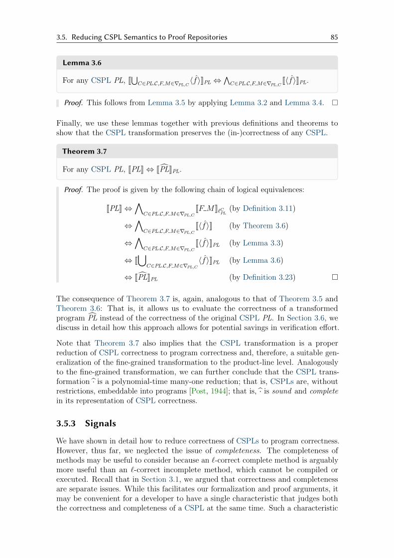
3.5. Reducing CSPL Semantics to Proof Repositories 85
Lemma 3.6
For any CSPL PL, J⋃C∈PL.C,F M∈∇PL,C 〈f〉KPL ⇔
∧C∈PL.C,F M∈∇PL,CJ〈f〉KPL.
Proof. This follows from Lemma 3.5 by applying Lemma 3.2 and Lemma 3.4.
Finally, we use these lemmas together with previous definitions and theorems toshow that the CSPL transformation preserves the (in-)correctness of any CSPL.
Theorem 3.7
For any CSPL PL, JPLK⇔ JPLKPL.
Proof. The proof is given by the following chain of logical equivalences:
JPLK⇔∧
C∈PL.C,F M∈∇PL,CJF MK`CPL (by Definition 3.11)
⇔∧
C∈PL.C,F M∈∇PL,CJ〈f〉K (by Theorem 3.6)
⇔∧
C∈PL.C,F M∈∇PL,CJ〈f〉KPL (by Lemma 3.3)
⇔ J⋃
C∈PL.C,F M∈∇PL,C〈f〉KPL (by Lemma 3.6)
⇔ JPLKPL (by Definition 3.23) �
The consequence of Theorem 3.7 is, again, analogous to that of Theorem 3.5 andTheorem 3.6: That is, it allows us to evaluate the correctness of a transformedprogram PL instead of the correctness of the original CSPL PL. In Section 3.6, wediscuss in detail how this approach allows for potential savings in verification effort.
Note that Theorem 3.7 also implies that the CSPL transformation is a properreduction of CSPL correctness to program correctness and, therefore, a suitable gen-eralization of the fine-grained transformation to the product-line level. Analogouslyto the fine-grained transformation, we can further conclude that the CSPL trans-formation · is a polynomial-time many-one reduction; that is, CSPLs are, withoutrestrictions, embeddable into programs [Post, 1944]; that is, · is sound and completein its representation of CSPL correctness.
3.5.3 Signals
We have shown in detail how to reduce correctness of CSPLs to program correctness.However, thus far, we neglected the issue of completeness. The completeness ofmethods may be useful to consider because an `-correct complete method is arguablymore useful than an `-correct incomplete method, which cannot be compiled orexecuted. Recall that in Section 3.1, we argued that correctness and completenessare separate issues. While this facilitates our formalization and proof arguments, itmay be convenient for a developer to have a single characteristic that judges boththe correctness and completeness of a CSPL at the same time. Such a characteristic
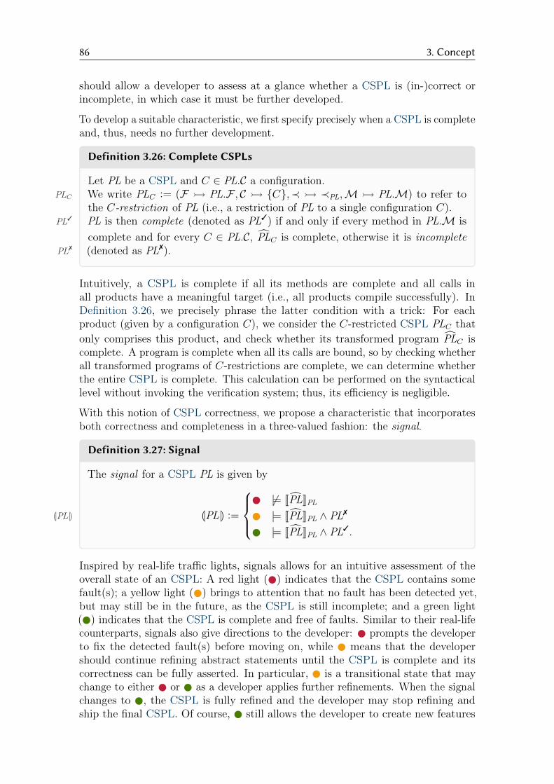
86 3. Concept
should allow a developer to assess at a glance whether a CSPL is (in-)correct orincomplete, in which case it must be further developed.
To develop a suitable characteristic, we first specify precisely when a CSPL is completeand, thus, needs no further development.
Definition 3.26: Complete CSPLs
Let PL be a CSPL and C ∈ PL.C a configuration.We writePLC PLC := (F � PL.F , C � {C},≺ � ≺PL,M � PL.M) to refer tothe C-restriction of PL (i.e., a restriction of PL to a single configuration C).PL is then complete (denoted asPL3 PL3) if and only if every method in PL.M is
complete and for every C ∈ PL.C, PLC is complete, otherwise it is incomplete(denoted asPL7 PL7).
Intuitively, a CSPL is complete if all its methods are complete and all calls inall products have a meaningful target (i.e., all products compile successfully). InDefinition 3.26, we precisely phrase the latter condition with a trick: For eachproduct (given by a configuration C), we consider the C-restricted CSPL PLC that
only comprises this product, and check whether its transformed program PLC iscomplete. A program is complete when all its calls are bound, so by checking whetherall transformed programs of C-restrictions are complete, we can determine whetherthe entire CSPL is complete. This calculation can be performed on the syntacticallevel without invoking the verification system; thus, its efficiency is negligible.
With this notion of CSPL correctness, we propose a characteristic that incorporatesboth correctness and completeness in a three-valued fashion: the signal.
Definition 3.27: Signal
The signal for a CSPL PL is given by
LPLM LPLM :=
6|= JPLKPL |= JPLKPL ∧ PL7
|= JPLKPL ∧ PL3.
Inspired by real-life traffic lights, signals allows for an intuitive assessment of theoverall state of an CSPL: A red light ( ) indicates that the CSPL contains somefault(s); a yellow light ( ) brings to attention that no fault has been detected yet,but may still be in the future, as the CSPL is still incomplete; and a green light( ) indicates that the CSPL is complete and free of faults. Similar to their real-lifecounterparts, signals also give directions to the developer: prompts the developerto fix the detected fault(s) before moving on, while means that the developershould continue refining abstract statements until the CSPL is complete and itscorrectness can be fully asserted. In particular, is a transitional state that maychange to either or as a developer applies further refinements. When the signalchanges to , the CSPL is fully refined and the developer may stop refining andship the final CSPL. Of course, still allows the developer to create new features

3.5. Reducing CSPL Semantics to Proof Repositories 87
and methods, in which case the signal may again change to , prompting for furtherrefinements.
We can determine the signal for our example CSPL PL in Figure 3.4 as follows: First,this CSPL is complete, as all its CbC trees are fully refined and every call in everyproduct has a meaningful target (as shown in Figure 3.7). Thus, LPLM ∈ { , }.Whether LPLM is or depends on whether we include the guard definition fromFigure 3.1: If we include the faulty guard definition, LPLM = ; if we use the correctedCbC tree instead, LPLM = as expected.
Defined this way, signals can easily be implemented in integrated developmentenvironments (IDEs) for CSPLs. In addition, this approach can also be implementedfor individual methods in a CSPL such that each method has its own signal. Whenevera developer makes a change (e.g., adding a refinement), the signal for the CSPL(or individual method) may be re-evaluated according to Definition 3.27. Thus,developers can constantly get feedback on their changes and use said feedback toissue new changes, which creates an interactive “conversation” between the developerand the IDE. In Chapter 5, we recount our initial experiences with this interactiveapproach.

88 3. Concept
3.6 DiscussionIn Section 3.4 and Section 3.5, we proposed several transformations from CSPLconcepts to program concepts with the goal to reduce CSPL correctness to programcorrectness. With Theorem 3.7, we have shown that · is indeed a correctness-preserving reduction from CSPLs to programs and, thus, achieved said goal. In thissection, we discuss how this reduction to program semantics (i.e., proof repositories)may allow for an overall reduction in verification effort. To this end, we discusstwo separate kinds of proof reuse that can be achieved with proof repositories. Thecombinations of these kinds of proof reuse then give rise to four distinct querystrategies for proof repositories with different use cases and (dis-)advantages. Wedefine and discuss each query strategy with respect to a classification introduced byThum et al. [2014a].
3.6.1 Proof ReuseProof reuse refers to an approach where we store existing (possibly partial) proofs,using them to prove several programs (or fragments thereof) at once [Bubel et al.,2016; Klebanov, 2007]. The absence of any proof reuse corresponds to a naiveproduct-based analysis, where each configuration is analyzed separately (as discussedin Section 3.2). The extent of proof reuse when utilizing proof repositories is twofold:That is, proof repositories allow for structural reuse (SR) and partial proof reuse(PPR). We distinguish both kinds of reuse because they are completely differentideas that are conveniently combined in the proof repository approach.
Structural Reuse. With structural reuse, we refer to the proof reuse that we canachieve just by how proof repositories are structured. Consider our example CSPLin Figure 3.4: The method List Insert occurs in all four configurations of the CSPL;thus, its correctness should be evaluated four times (once for each configuration) ina product-based analysis. However, on close inspection, we observe that List Insertdoes not contain any method calls and is therefore identical in all four configurations.Thus, it would be sensible to analyze List Insert only once, as there is only one truevariant of this method in the CSPL. In general, we say that an analysis accomplishesstructural reuse when it detects and avoids redundant invocations of the verificationsystem.
This is automatically the case whenever we employ proof repositories: By the defini-tion of sound proof repository domains (cf. Definition 3.16), the precise circumstancesfor each proof are tracked. Because of duplicate elimination in sets (on which ourformalization is based), several proof descriptors with the same circumstances (i.e.,implementation and set of bindings) always collapse to a single proof in the soundproof repository. For example, in Figure 3.18, the method List Insert gives rise to asingle proof descriptor (I � IList Insert ,B� ∅) for each configuration. Because thisproof descriptor is identical for all configurations, it collapses to one under the unionof sets in Definition 3.16. Intuitively, this means that proof repositories evaluate thecorrectness for each true variant of a method (e.g., by differing contracts or calls)only once, which eliminates some redundancy.
Partial Proof Reuse. With partial proof reuse, we refer to the proof reuse accomplishedby using a verification system that supports partial proofs. To exemplify this, let
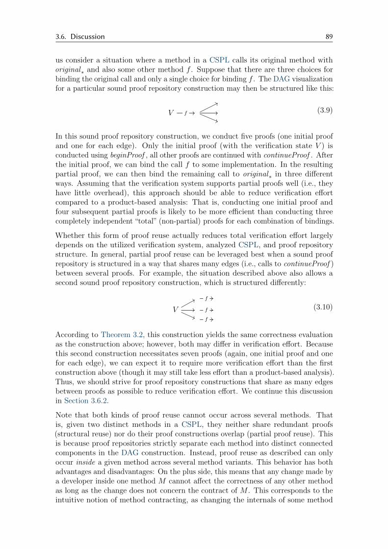
3.6. Discussion 89
us consider a situation where a method in a CSPL calls its original method withoriginal∗ and also some other method f . Suppose that there are three choices forbinding the original call and only a single choice for binding f . The DAG visualizationfor a particular sound proof repository construction may then be structured like this:
V f (3.9)
In this sound proof repository construction, we conduct five proofs (one initial proofand one for each edge). Only the initial proof (with the verification state V ) isconducted using beginProof , all other proofs are continued with continueProof . Afterthe initial proof, we can bind the call f to some implementation. In the resultingpartial proof, we can then bind the remaining call to original∗ in three differentways. Assuming that the verification system supports partial proofs well (i.e., theyhave little overhead), this approach should be able to reduce verification effortcompared to a product-based analysis: That is, conducting one initial proof andfour subsequent partial proofs is likely to be more efficient than conducting threecompletely independent “total” (non-partial) proofs for each combination of bindings.
Whether this form of proof reuse actually reduces total verification effort largelydepends on the utilized verification system, analyzed CSPL, and proof repositorystructure. In general, partial proof reuse can be leveraged best when a sound proofrepository is structured in a way that shares many edges (i.e., calls to continueProof )between several proofs. For example, the situation described above also allows asecond sound proof repository construction, which is structured differently:
V
f
f
f
(3.10)
According to Theorem 3.2, this construction yields the same correctness evaluationas the construction above; however, both may differ in verification effort. Becausethis second construction necessitates seven proofs (again, one initial proof and onefor each edge), we can expect it to require more verification effort than the firstconstruction above (though it may still take less effort than a product-based analysis).Thus, we should strive for proof repository constructions that share as many edgesbetween proofs as possible to reduce verification effort. We continue this discussionin Section 3.6.2.
Note that both kinds of proof reuse cannot occur across several methods. Thatis, given two distinct methods in a CSPL, they neither share redundant proofs(structural reuse) nor do their proof constructions overlap (partial proof reuse). Thisis because proof repositories strictly separate each method into distinct connectedcomponents in the DAG construction. Instead, proof reuse as described can onlyoccur inside a given method across several method variants. This behavior has bothadvantages and disadvantages: On the plus side, this means that any change made bya developer inside one method M cannot affect the correctness of any other methodas long as the change does not concern the contract of M . This corresponds to theintuitive notion of method contracting, as changing the internals of some method

90 3. Concept
SR PPR Classification
Exhaustive } Feature-Family-BasedLate-Splitting
Complete # Optimized Product-BasedProduct-Based # # Unoptimized Product-Based
Figure 3.20: Query strategies for CSPL correctness.
should not affect other methods. In an IDE, this means that when a developer editsa given method without changing its contract, only the signal for said method mustbe displayed and re-calculated. However, there is also a downside to this behavior:Namely, proof repositories (as described in this thesis) cannot leverage similaritiesbetween distinct methods; for example, when two methods have identical contractsand implementations. Another scenario where proof repositories do not provideproof reuse is when a method M calls another method M ′, of which there are twovariants with the same contract. Intuitively, because both variants of M ′ have thesame contract, we only have to conduct a single proof for M binding M ′ accordingly.However, because proof repositories strictly separate different methods, they cannotdetect and leverage this circumstance.
3.6.2 �ery StrategiesIn Definition 3.18, we described how we can evaluate a program’s correctness usingits sound proof repository: That is, a program is correct when all complete proofs inits sound proof repository are closable as well (this also applies to our pruning schemefor CSPLs in Definition 3.25). In this section, we discuss four query strategies forsound proof repositories that we can use to evaluate program correctness (and, perTheorem 3.7, CSPL correctness). Not all of these query strategies utilize structuraland partial proof reuse as discussed in Section 3.6.1; in fact, both kinds of proofreuse can be combined in three different ways. In Figure 3.20, we show all querystrategies, the kinds of proof reuse they permit, and how we classify them accordingto a classification of SPL analysis strategies by Thum et al. [2014a]. We start bydiscussing the exhaustive strategy, which is the simplest of the four.
Exhaustive. In this strategy, we calculate the entire sound proof repository for aCSPL before querying it (thus, exhaustive). That is, for any CSPL PL, we calculate
its CSPL-transformed program PL and corresponding sound proof repository RPLPL.
Afterwards, we determine whether each complete proof descriptor in RPLPL maps to a
closable verification state, in which case PL is correct. As discussed in Section 3.6.1,this strategy utilizes proof repositories and therefore allows for structural reuse.Because we also use partial proofs as described in Definition 3.14, this strategy alsopermits partial proof reuse.
With regard to the classification by Thum et al., we consider this to be a feature-family-based analysis. Put briefly, a feature-family-based analysis is a feature-basedanalysis followed by a family-based analysis, where the latter must depend on theresults of the former. A feature-based analysis may only analyze the artifacts ofan SPL (not its products) and must analyze these artifacts in isolation (without

3.6. Discussion 91
considering configurations or feature interactions [Bowen et al., 1989]). A family-based analysis also operates on SPL artifacts only (not on products), but it mayconsider configurations and feature interactions.
We believe the exhaustive strategy to be a feature-family-based analysis becausewe can divide it in two phases, where the latter phase depends on the first: In thefirst phase (corresponding to the base case in Definition 3.17), we calculate a singleinitial proof for each implementation in the transformed program with beginProof .Intuitively, these are the proofs to the far left in our DAG visualizations (e.g.,Figure 3.19). As we already discussed in Section 3.6.1, these proofs span distinctconnected components in the DAG structure. That is, we can conduct these initialproofs in isolation (or even in parallel) as they do not use any bindings (i.e., knowledgeabout configurations) yet. We further do not analyze any specific products in thisphase, which makes it a feature-based analysis. On the other hand, the second phase(corresponding to the induction step) explicitly addresses all the interactions betweenfeatures and incorporates knowledge about configurations (in form of bindings). Still,we only analyze artifacts on the CSPL level and no individual products, which makesthis phase a family-based analysis. In summary, the exhaustive query strategy firstconducts isolated initial proofs for all methods and then continues these proofs withknowledge from the feature model and other methods; thus, it meets the criteria fora feature-family-based analysis.
Late-Spli�ing. The exhaustive query strategy discussed above is simple to implement(provided a suitable verification system with support for partial proofs). However,it somewhat contradicts our goal, namely reducing the overall verification effort.Consider again Figure 3.19, where we show twelve proofs related to the methodSet Insert (pruned proofs already omitted). Note that, of these twelve proofs, onlytwo are actually complete (marked with (3, 3)). Consequently, to evaluate thecorrectness of this particular method, we actually only need to compute these twoproofs. To this end, we could choose any two paths in the DAG visualization thatlead to these proofs, and only conduct the proofs lying on these paths:
(7,7) (7,7) (7,7) (3,3)Set Insert
(7,7)(7,7) (3,3)
cP (·,B1) cP (·,B8) cP (·,B3)cP(·,B6)
cP (·,B5)cP (·,B7)
By only conducting the seven proofs on these two paths (and omitting the other fiveproofs), we can reduce the overall verification effort, without sacrificing any accuracyin our analysis. This is the basic idea of our late-splitting query strategy: In thisstrategy, we aim to omit all proofs that do not directly contribute to the goal ofour analysis (i.e., evaluating CSPL correctness). In principle, this strategy works
as follows for any CSPL PL, its CSPL-transformed program PL, and corresponding
sound proof repository domain DPLPL: First, we identify all complete proof descriptors
in DPLPL. Next, for each such proof descriptor D, we choose some path in the DAG
that starts at (I � D.I,B � ∅) and leads to D. Finally, we conduct all proofson all chosen paths and evaluate the correctness of PL on the resulting sound proofrepository, analogously to the exhaustive query strategy.
It is not immediately obvious, however, how to choose a path in the DAG, as theremight be many and some might be more efficient than others in terms of verification

92 3. Concept
effort (cf. Theorem 3.2). As a reasonable heuristic to choose paths, we introduce anidea that we refer to as late splitting (named after a similar idea proposed by Apel et al.[2013b]): Basically, we prefer to choose paths that share as many edges as possible;thus, maximizing the partial proof reuse (as already demonstrated in Section 3.6.1).We refer to this heuristic as late-splitting because it favors combinations of pathsthat have a maximum common prefix; or, intuitively, because it prefers when pathssplit late (3.9) rather than early (3.10). We omit the details of this late-splittingheuristic, as it is a fairly simple graph algorithm that does not contribute anythingsubstantial to our discussion. In summary, the late-splitting query strategy omitscertain proofs (determined with a heuristic) that do not contribute to the analysisgoal to reduce the overall verification effort.
Compared to the exhaustive query strategy, this strategy is advantageous when weare only interested in evaluating a CSPL’s correctness once. In an evolution scenario,however, the exhaustive query strategy might be preferable because it proactivelyconducts more proofs, which may or may not be needed in the future. In terms ofproof reuse and classification according to Thum et al., late-splitting has the sameproperties as the exhaustive query strategy (cf. Figure 3.20).
Complete. With the late-splitting query strategy, we demonstrated how we can omitcertain proofs to reduce the overall verification effort. However, we can still takethis approach a little further: After all, only complete proofs contribute to our goalof evaluating CSPL correctness, and in the late-splitting query strategy, we stillconduct some incomplete proofs. Instead, we may try to omit all incomplete proofsas well and conduct only complete proofs (in case of Set Insert, the two proofsmarked with (3, 3) above). However, to do so, we must sacrifice all partial proofreuse and conduct classical “total” proofs instead. That is, instead of the exhaustiveor late-splitting query strategy (for which we would conduct twelve or five proofs,respectively), we conduct only two proofs for the complete query strategy. However,these proofs do not benefit from partial proof reuse at all and may therefore containmutually redundant proof steps, which may have negative impact on verificationeffort. Thus, it is not immediately obvious whether this query strategy performsbetter or worse than the exhaustive or late-splitting query strategies. We discussthis further in our evaluation in Chapter 5.
When we take a closer look at this strategy, we can observe that it essentially proveseach variant of each method in a CSPL once. For instance, there are two variantsof Set Insert in our example CSPL, one for unordered (cf. Figure 3.7c) and onefor ordered sets (cf. Figure 3.7c), and the two conducted proofs in this strategydirectly correspond to these variants. Thus, this strategy allows for structural, butnot partial proof reuse (cf. Figure 3.20). In the classification by Thum et al., thecomplete query strategy can be considered an optimized product-based analysis. Thisis because this strategy essentially conducts the same proofs as a naive product-basedanalysis (cf. Section 3.2); however, it still avoids redundant proofs through structuralreuse by utilizing proof repositories and, thus, it meets the criteria for an optimizedproduct-based analysis.
Product-Based. The last of the four query strategies we propose is a product-basedquery strategy, which corresponds to an unoptimized product-based analysis accordingto Thum et al. and does not allow for any proof reuse (cf. Figure 3.20). We propose
3.6. Discussion 93
this strategy mainly as a baseline for comparison with the first three strategies in ourevaluation in Chapter 5. Nonetheless, it is a valid query strategy on its own becauseit may perform well especially for very small CSPLs.
To keep the first three strategies comparable with the product-based query strategy,we make use of the following fact: Instead of evaluating the correctness of a CSPLas a whole, we can just evaluate the correctness of each of its products separately.With a trick, we can then implement this strategy with proof repositories as follows:For any CSPL PL and configuration C ∈ PL.C, calculate the C-restriction of PLand its CSPL-transformed program PLC . Then, evaluate the correctness for each ofthese transformed programs, analogously to the complete query strategy; PL is thencorrect when all transformed programs are correct. Thus, the product-based querystrategy can be considered a variant of the complete query strategy that we applyseparately on each product of the CSPL. This way, it is comparable with the firstthree strategies and can easily be implemented alongside them.
This concludes our discussion of query strategies for sound proof repositories. Wecontinue to discuss these strategies in Chapter 4 and Chapter 5, where we implementand evaluate them. Note that, save for the product-based query strategy, our querystrategies are also applicable outside the context of CSPLs or FOP-based SPLs;namely, we can apply them in any scenario involving proof repositories (e.g., classinheritance and behavioral subtyping as proposed by Bubel et al. [2016]). Similarly,our discussion of proof reuse also applies to proof repositories in general.

94 3. Concept
SPLs(3.2)
CbC(3.1)
PRs(3.3)
CSPLs(3.2)
c(3.4.1)
f(3.4.2)
PL(3.5)
Figure 3.21: Overview of our contributions in this chapter.
3.7 SummaryIn this chapter, we proposed a novel feature-family-based analysis for evaluatingthe correctness of CSPLs. Our analysis is based on and extends the previouslyproposed proof repository approach [Bubel et al., 2016], which aims to facilitateverification-in-the-large. In particular, our proposed analysis is sound and completeand can therefore transparently replace a product-based analysis, while potentiallyreducing the overall verification effort. In the following, we recapitulate the structureand contextualize the contributions of this chapter (cf. Figure 3.21).
In Section 3.1, 3.2, and 3.3, we laid the formal foundations for our contributionsin Section 3.4, 3.5, and 3.6. We introduced the CbC methodology and CbC treesin Section 3.1 and continued with SPL concepts in Section 3.2, where we discussedmethod calls and lookups. By linking CbC with SPL concepts, we formalized CSPLs(following previous work by Bordis et al. [2020b]) and their semantics, which serve asa baseline so we can judge the soundness and completeness of our analysis. Next, wedescribed proof repositories (following Bubel et al. [2016]), which promise proof reusefor the verification of large programs by decoupling a method call from its target. Inour description, we contributed several extensions and insights, which (besides beinguseful for our application to CSPLs) we believe to be a consistent further developmentof the proof repository approach. Together, CbC, CSPLs, and proof repositoriescomprise the subject matter for the development of our feature-family-based analysisin Section 3.4 and 3.5.
Our general approach was to map CSPL concepts into program (and, thus, proofrepository) concepts in a way that completely preserves the (in-)correctness of CSPLs.We summarize the resulting mapping in Figure 3.22, where each row names onetransformation and show its parameters, result, direction, and where it is defined.We arrived at this mapping in two separate steps: First, we considered how totransform a single method in a CSPL into a program in Section 3.4. We observedthat there are two opposing philosophies to transforming methods, depending on the
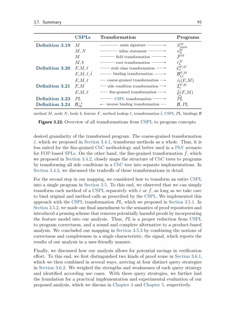
3.7. Summary 95
CSPLs Transformation Programs
Definition 3.19 M main signature SMmain
M,N inline statement sMNM field transformation FMM, b root transformation rMb
Definition 3.20 F M, ` stub class transformation CF M`
F M, `, t binding transformation BF M`,t
F M, ` coarse-grained transformation c`(F M)Definition 3.21 F M side condition transformation IF M
∗F M, ` fine-grained transformation f`(F M)
Definition 3.23 PL CSPL transformation PLDefinition 3.24 B−1PL
inverse binding transformation B,PL
method M , node N , body b, feature F , method lookup `, transformation t, CSPL PL, bindings B
Figure 3.22: Overview of all transformations from CSPL to program concepts.
desired granularity of the transformed program: The coarse-grained transformationc, which we proposed in Section 3.4.1, transforms methods as a whole. Thus, it isless suited for the fine-grained CbC methodology and better used in a PhV scenariofor FOP-based SPLs. On the other hand, the fine-grained transformation f , whichwe proposed in Section 3.4.2, closely maps the structure of CbC trees to programsby transforming all side conditions in a CbC tree into separate implementations. InSection 3.4.3, we discussed the tradeoffs of these transformations in detail.
For the second step in our mapping, we considered how to transform an entire CSPLinto a single program in Section 3.5. To this end, we observed that we can simplytransform each method of a CSPL separately with c or f , as long as we take careto bind original and method calls as prescribed by the CSPL. We implemented thisapproach with the CSPL transformation PL, which we proposed in Section 3.5.1. InSection 3.5.2, we made one final amendment to the semantics of proof repositories andintroduced a pruning scheme that removes potentially harmful proofs by incorporatingthe feature model into our analysis. Thus, PL is a proper reduction from CSPLto program correctness, and a sound and complete alternative to a product-basedanalysis. We concluded our mapping in Section 3.5.3 by combining the notions ofcorrectness and completeness in a single characteristic, the signal, which reports theresults of our analysis in a user-friendly manner.
Finally, we discussed how our analysis allows for potential savings in verificationeffort. To this end, we first distinguished two kinds of proof reuse in Section 3.6.1,which we then combined in several ways, arriving at four distinct query strategiesin Section 3.6.2. We weighed the strengths and weaknesses of each query strategyand identified according use cases. With these query strategies, we further laidthe foundation for a practical implementation and experimental evaluation of ourproposed analysis, which we discuss in Chapter 4 and Chapter 5, respectively.


4. Implementation
In Chapter 3, we gave a comprehensive formal description of our feature-family-basedanalysis for CSPL correctness. We implement this analysis on top of the deductiveverification system KeY in a prototype named KeYPR (KeY for Proof Repositories),which is publicly available in our GitHub repository.1 In this chapter, we describeour prototype and illustrate its mode of operation with an example.
Before, we deliberately omitted the discussion of some practical issues to ensurethat our analysis is applicable to a variety of languages and verification systems.With KeYPR, we instead focus on Java programs and contracts specified with JML,similar to Bubel et al. [2016] and Runge et al. [2019a]. Thus, we need a verificationsystem for Java/JML that conforms to Definition 3.14. Like Bubel et al. and Rungeet al., we choose KeY for this task, which is a platform for verifying Java programsagainst JML contracts [Ahrendt et al., 2014, 2016; Beckert et al., 2007]. However,the default distribution of KeY does not support partial proofs. This is why weinstead decided to use a modified variant of KeY 2.1 that is enhanced with abstractcontracts, a mechanism for partial proofs [Bubel et al., 2014; Hahnle et al., 2013;Pelevina, 2014]. We ported this modified variant to the latest version of KeY 2.7 (asof June 2020) to benefit from all its optimizations and new features. Note that weomit the technical details of abstract contracts described by Pelevina; instead, wefocus on their application within KeYPR.
In Figure 4.1, we show that KeYPR operates in several phases, which take a codedrepresentation of a CSPL and yield its signal according to Definition 3.27. Notethat this pipeline can be applied in an iterative fashion; in fact, developers areeven encouraged to do so following the CbC methodology. A typical developmentexperience with KeYPR may therefore look like this: A developer may start withan empty CbC tree for some method and run KeYPR to find that the CbC tree iscorrect (cf. Definition 3.10). Next, they may refine some abstract statement and runKeYPR again to find that, say, their refinement introduced a fault into the CbC tree.They may investigate the problem (as discussed in Section 3.4.3) and update their
1Available at: https://github.com/ekuiter/KeYPR

98 4. Implementation
Parse CSPLfrom DSL
CalculatePR Domain
GenerateCode
ConductProofs
CalculateSignal
Figure 4.1: Pipeline for evaluating CSPL correctness with KeYPR.
refinement, running KeYPR again to find that, say, their refinement is now correct.This feedback cycle may repeat indefinitely, which is only possible because we alsoconsider the correctness of incomplete CbC trees and methods in Section 3.2.2. Withappropriate IDE integration, this approach allows for an interactive conversationbetween the developer and the IDE that supports the CbC methodology [Rungeet al., 2019b]. Even without proper IDE integration (which KeYPR lacks as of now)it is still quite easy to derive a correct CbC tree in an interactive fashion due to ourtechnological choices, as we discuss below.
We demonstrate the inner workings of our prototype for an excerpt of our exampleCSPL in Figure 3.4. In particular, we proceed to discuss the method MList Insert
according to the phases shown in Figure 4.1.
Parse CSPL from DSL. In this first phase, KeYPR takes the developer’s input andtransforms it into an internal representation suitable for further processing in thenext phases. For reasons that we discuss below, we choose the Clojure programminglanguage [Hickey, 2008] to implement the concept we proposed in Chapter 3. Notethat Clojure is a Lisp dialect and therefore homoiconic, which means that there isbarely a distinction between code and data [McIlroy, 1960]; thus, Clojure can easilyparse and evaluate code written in itself. We leverage this property to define a simple,but powerful domain-specific language (DSL) for expressing CbC trees, methods,and entire CSPLs.
We exemplify this DSL in Figure 4.2, where we show the full CbC tree for MList Insert ,which we derived with the iterative approach discussed above. We embed MList Insert
into an (otherwise empty) scaffold for expressing the entire example CSPL fromFigure 3.4. Thus, Figure 4.2 also shows a snapshot of an early development stageof said CSPL. Note that the syntax of our DSL closely resembles our definitionsfrom Chapter 3. For example, a CSPL ({Fi}, {Ci},≺, {Mi}) can be expressed as(CSPL [F1 ...] [C1 ...] [] [] [M1 ...]), where the feature order ≺ is already en-coded in [F1 ...]. The two empty vectors [] [] encode additional settings (e.g.,strategy settings for KeY) as well as macros (i.e., convenient substitutions forfrequent FOL formulas). Similarly, methods and CbC trees can be expressedwith (M ...) and (T ...), where signatures can be supplied in a string represen-tation (e.g., "int[] ::List_Insert(int[] A, int x)") and local variables as vectors(e.g., ["int" "i"] for a local integer variable i). Due to Clojure’s code manipulationcapabilities, we can express a CbC tree in a hierarchical fashion, where (=> ...)
marks a refinement and each kind of statement in Definition 3.1 has its own syntax(e.g., (repetition I V G) for a repetition with invariant I, variant V , and guard G).Compared to a fully-fledged IDE like VarCorC [Bordis et al., 2020b; Kodetzki, 2020],this representation of CSPLs has some advantages: First, it is lightweight (the DSLtakes ≈ 50 SLOC), while allowing for reasonably intuitive usage nonetheless. Inaddition, we can leverage Clojure’s read-eval-print loop (REPL) (which is similar toa command line interface) to allow for interactive usage as described above as well.

99
(CSPL
["List" "Ordered" "Set"]
[["List"] ["List" "Ordered"] ["List" "Set"] ["List" "Ordered" "Set"]]
[[:strategy-property "NON_LIN_ARITH_OPTIONS_KEY = NON_LIN_ARITH_DEF_OPS"]]
[["in($A, $i)" ((in 0 :<= :<= "$A.length") "$i")]
["appAllIn($A’, $i, $j, $A)"
(forall (in "$i" :<= :< "$j") #(format "appIn($A’, $A[%s], $i, $j)" %))]
["appAll($A’, $A)" (forall (in "$A") #(format "app($A’, $A[%s])" %))]
["app($A, $x)" "appIn($A, $x, 0, $A.length)"]
["appIn($A, $x, $i, $j)"
(exists (in "$i" :<= :< "$j") #(format "$A[%s] == $x" %))]]
[(M "int[] ::List_Insert(int[] A, int x)"
"Inserts an integer into a list."
[["int" "i"]]
(T "A.length > 0" "app(_result, x) && appAll(_result, A)"
(let [inv (str "_result.length == A.length + 1"
" && _result[_result.length - 1] == x"
" && in(A, i) && appAllIn(_result, 0, i, A)")]
(=> (abstract-statement)
(=> (composition (str inv " && i == 0"))
(=> (assignment ["i" "_result" "_result[_result.length-1]"]
["0" "new int[A.length + 1]" "x"]))
(=> (repetition inv "A.length - i" "i < _result.length")
(=> (assignment ["_result[i]" "i"]
["A[i]" "i + 1"]))))))))])
Figure 4.2: Implementation of the CSPL in Figure 3.4 with the KeYPR DSL.
Calculate Proof Repository Domain. Based on the internal representation of a CSPL
PL, KeYPR calculates its pruned proof repository domain DPLPL next. Depending on
the utilized query strategy, this is also where a selection of the conducted proofs (e.g.,for late-splitting) may take place. We implement the entire business logic for CbC,CSPLs, and proof repositories as well as all transformations from Chapter 3 in Clojureas mentioned above. The reason why we choose Clojure (instead of, for example,Java) for this task is that Clojure has deep integration for immutable persistent datastructures, which allow for a functional programming style that closely resemblesour original definitions. Thus, our code2 is short and concise (≈ 250 SLOC) andless likely to contain implementation errors than if we had chosen another, moreimperative language (like Java). Clojure has the additional advantage that it runson the Java virtual machine (JVM), which facilitates interaction with KeY.
Generate Code. With the pruned proof repository domain at hand, we can movetowards conducting the actual proofs to build the pruned proof repository. As wewant to use KeY to conduct individual proofs, we must either generate a .problem
file for KeY or a .java class that models the program fragment we want to verify.Because of the way abstract contracts are implemented in our version of KeY, we optfor the latter approach (in contrast to VarCorC, which directly generates .problem
files without using abstract contracts). Because an imperative language is betterfitted for this code generation task, we implement it in Java, interfacing with the
2Annotated source code for the functional core is available at:https://github.com/ekuiter/KeYPR/blob/master/src/main/clojure/de/ovgu/spldev/keypr.clj
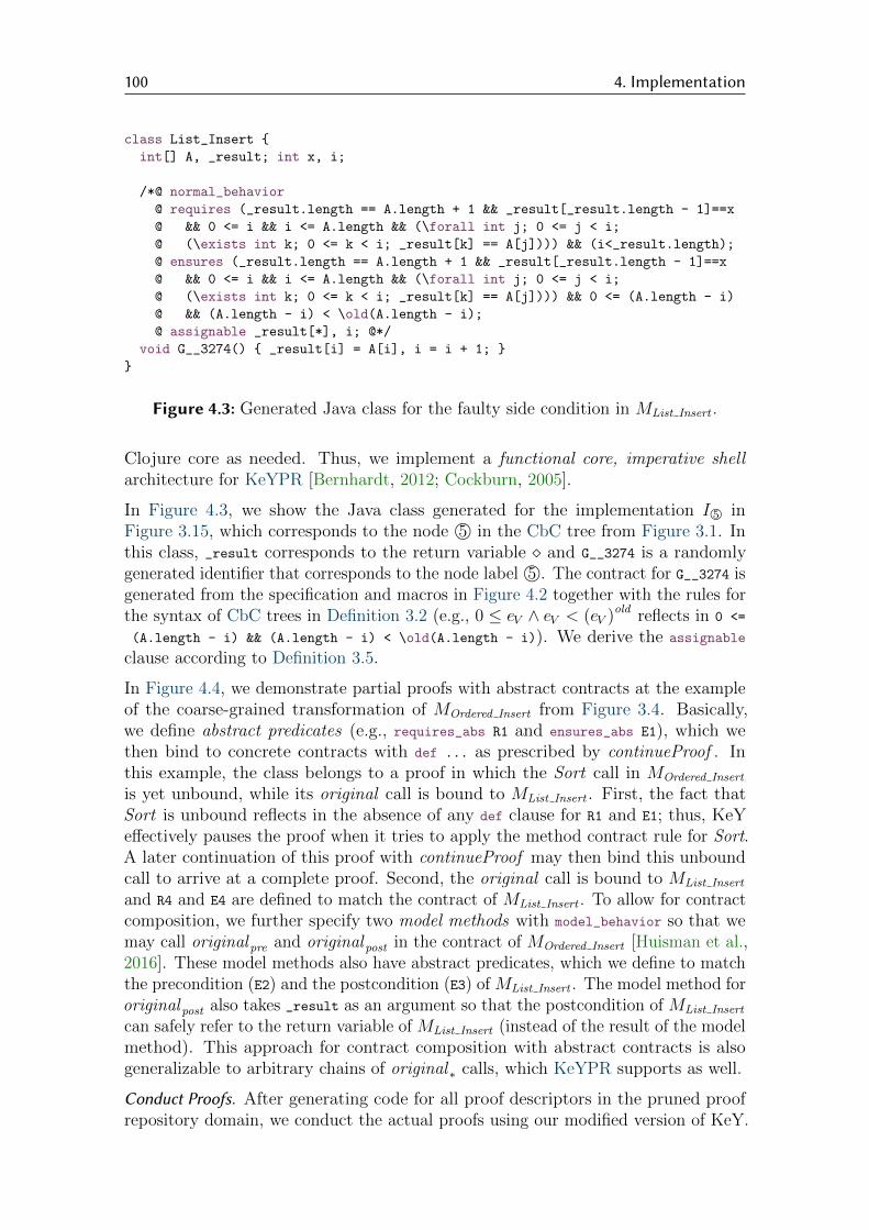
100 4. Implementation
class List_Insert {
int[] A, _result; int x, i;
/*@ normal_behavior
@ requires (_result.length == A.length + 1 && _result[_result.length - 1]==x
@ && 0 <= i && i <= A.length && (\forall int j; 0 <= j < i;
@ (\exists int k; 0 <= k < i; _result[k] == A[j]))) && (i<_result.length);
@ ensures (_result.length == A.length + 1 && _result[_result.length - 1]==x
@ && 0 <= i && i <= A.length && (\forall int j; 0 <= j < i;
@ (\exists int k; 0 <= k < i; _result[k] == A[j]))) && 0 <= (A.length - i)
@ && (A.length - i) < \old(A.length - i);
@ assignable _result[*], i; @*/
void G__3274() { _result[i] = A[i], i = i + 1; }
}
Figure 4.3: Generated Java class for the faulty side condition in MList Insert .
Clojure core as needed. Thus, we implement a functional core, imperative shellarchitecture for KeYPR [Bernhardt, 2012; Cockburn, 2005].
In Figure 4.3, we show the Java class generated for the implementation I 5© inFigure 3.15, which corresponds to the node 5© in the CbC tree from Figure 3.1. Inthis class, _result corresponds to the return variable � and G__3274 is a randomlygenerated identifier that corresponds to the node label 5©. The contract for G__3274 isgenerated from the specification and macros in Figure 4.2 together with the rules forthe syntax of CbC trees in Definition 3.2 (e.g., 0 ≤ eV ∧ eV < (eV )old reflects in 0 <=
(A.length - i) && (A.length - i) < \old(A.length - i)). We derive the assignable
clause according to Definition 3.5.
In Figure 4.4, we demonstrate partial proofs with abstract contracts at the exampleof the coarse-grained transformation of MOrdered Insert from Figure 3.4. Basically,we define abstract predicates (e.g., requires_abs R1 and ensures_abs E1), which wethen bind to concrete contracts with def ... as prescribed by continueProof . Inthis example, the class belongs to a proof in which the Sort call in MOrdered Insert
is yet unbound, while its original call is bound to MList Insert . First, the fact thatSort is unbound reflects in the absence of any def clause for R1 and E1; thus, KeYeffectively pauses the proof when it tries to apply the method contract rule for Sort.A later continuation of this proof with continueProof may then bind this unboundcall to arrive at a complete proof. Second, the original call is bound to MList Insert
and R4 and E4 are defined to match the contract of MList Insert . To allow for contractcomposition, we further specify two model methods with model_behavior so that wemay call originalpre and originalpost in the contract of MOrdered Insert [Huisman et al.,2016]. These model methods also have abstract predicates, which we define to matchthe precondition (E2) and the postcondition (E3) of MList Insert . The model method fororiginalpost also takes _result as an argument so that the postcondition of MList Insert
can safely refer to the return variable of MList Insert (instead of the result of the modelmethod). This approach for contract composition with abstract contracts is alsogeneralizable to arbitrary chains of original∗ calls, which KeYPR supports as well.
Conduct Proofs. After generating code for all proof descriptors in the pruned proofrepository domain, we conduct the actual proofs using our modified version of KeY.

101
class Ordered_Insert {
int[] A, _result; int x;
/*@ normal_behavior
@ requires_abs R1;
@ ensures_abs E1;
@ assignable \nothing; @*/
int[] Sort_in_main_body(int[] _1) {}
/*@ model_behavior
@ ensures_abs E2;
@ def E2 = \result == (A.length > 0);
@ model boolean original_pre_in_main_contract(int[] A, int x) {} @*/
/*@ model_behavior
@ ensures_abs E3;
@ def E3 = \result == ((\exists int j; 0 <= j < _result.length; ...) && ...);
@ model boolean original_post_in_main_contract
(int[] _result, int[] A, int x) {} @*/
/*@ normal_behavior
@ requires_abs R4;
@ def R4 = A.length > 0;
@ ensures_abs E4;
@ def E4 = (\exists int j; 0 <= j < _result.length; ...) && ...;
@ assignable \nothing; @*/
int[] original_in_main_body(int[] A, int x) {}
/*@ normal_behavior
@ requires original_pre_in_main_contract(A, x) && ...;
@ ensures original_post_in_main_contract(_result, A, x) && ...;
@ assignable _result; @*/
int[] main(int[] A, int x) {
_result = original_in_main_body(A, x);
return Sort_in_main_body(_result);
}
}
Figure 4.4: Generated Java class with abstract contracts for MOrdered Insert .
To this end, we utilize the Java class KeYBridge in KeYPR. As input, this classtakes a proof descriptor, its generated code, and whether abstract contracts shouldbe used (depending on the selected query strategy). Then, this class automaticallyruns a proof strategy of KeY to find a proof. Notably, we offer three different modesof operation for abstract contracts, which we refer to as optimization strategies:none, default, and strict. We derived these optimization strategies from the modifiedvariant KeY 2.1 implemented by Pelevina [2014]. Note that when partial proofs areconducted in this variant of KeY, abstract predicates are explicitly forbidden to beexpanded as long as their calls are unbound. However, this means that KeY willtry to apply other rules instead, which may lead to many unnecessary proof stepsand new opened proof obligations (corresponding to the none optimization strategy).Pelevina addressed this by disabling certain rules regarding proof cuts and splits (thedefault optimization strategy) and the simplification of first-order goals (the strict

102 4. Implementation
optimization strategy). Because the tradeoffs between these optimization strategiesare not immediately obvious, we implement all of them in KeYPR and compare themin Chapter 5.
Calculate Signal. Finally, after all proofs have been conducted, KeYPR (in its Clojureportion of code) evaluates the completeness and correctness of the given CSPL PL.Completeness is a syntactical property that can easily be derived by inspectingthe internal representation of a CSPL. Correctness is then easily determined bychecking whether of all conducted proofs, those that are complete are also closable(cf. Definition 3.25). With this information, KeYPR calculates the signal LPLM andyields it to the developer, along with diagnostic information as to which conductedproofs succeeded and which failed.
This concludes our discussion of the KeYPR pipeline shown in Figure 4.1. A developermay then continuously repeat this process to apply more refinements to a CbC treeor correct faults in a previous refinement. With proper IDE integration, this entireprocess may be completely hidden from the developer behind an intuitive signal, orexposed in any level of detail to provide the developer with debugging information.

5. Evaluation
In Chapter 3 and Chapter 4, we proposed a feature-family-based analysis for evaluat-ing CSPL correctness and described a prototypical implementation. In this chapter,we investigate whether our analysis actually allows for a reduction in verificationeffort. We do so by an empirical evaluation on a small case study, which we developinteractively with our prototype.
5.1 Study DesignTo evaluate the verification effort of our analysis, we first define concrete researchquestions. To answer these questions, we then develop a case study with our prototypeand describe the experimental setup for our evaluation.
Research �estions. With our evaluation, we want to address the following questions:
RQ1 Is it feasible to create CSPLs and guarantee their correctness with our analysis?
RQ2 Does the choice of parameters influence the required verification effort of ouranalysis, and if so, how?
RQ3 Does our analysis reduce verification effort compared to previous approachesfor guaranteeing CSPLs correctness?
With these questions, we aim to evaluate the feasibility and efficiency of our analysisand compare it with other approaches. We intend to answer these questions withour prototypical implementation KeYPR according to the following methodology:
RQ1 We construct a CSPL case study with KeYPR in an incremental fashion. Inour construction, we make an intentional mistake, observe whether KeYPR canactually detect it (as predicted by Theorem 3.7), and fix it afterwards.
RQ2 We compute several proof repositories for the case study from RQ1 and measurethe required verification effort. We then compare how KeYPR performs for thefollowing parameters: Transformation (coarse- or fine-grained, cf. Section 3.4),query strategy (exhaustive, late-splitting, complete, or product-based, cf. Sec-tion 3.6.2), and optimization strategy (strict, default, or none, cf. Chapter 4).
104 5. Evaluation
RQ3 We compare the verification effort required by KeYPR with that required bypreviously proposed approaches.
Experimental Setup. To perform the evaluation, we run our prototype KeYPR on anotebook with an Intel Core i7-8650U 1.9 GHz processor and 16 GB of RAM. Toanswer RQ1, we incrementally develop a case study and give a subjective assessmenton the usability and performance of our prototype for this task. To answer RQ2 andRQ3, we evaluate the correctness of the case study CSPL we develop for RQ1 usingall possible combinations (or runs) of the parameters mentioned above. We arrive at16 runs, which we list in the appendix (cf. Figure A.1).
To measure the required verification effort, we rely on two metrics: We count thenumber of proof steps (also referred to as proof nodes) and measure the verificationtime elapsed during a proof. Both metrics are commonly used to quantify verificationeffort [Ahrendt et al., 2016; Knuppel et al., 2018]. The major advantage of the proofnode metric is that it is stable across computers and, thus, reproducible. However,proof nodes are an abstract quantity that does not represent verification effortintuitively. Thus, we also consider verification time, which is not as reproducible asproof nodes, but it is a more practical estimation of verification effort. Both proofnodes and verification time are measured by KeY automatically for each individualconducted proof. In addition, we measure the total verification time for one runwith standard Java facilities, which includes all time spent in the KeYPR pipelinediscussed in Chapter 4. By subtracting the verification time spent in KeY from thetotal time spent in KeYPR, we can calculate the overhead time that is spent onlyon bookkeeping tasks (e.g., calculating the proof repository and generating code forproofs).
Recall that, to answer RQ2 and RQ3, we use the corrected version of our case studyfrom RQ1. Because our case study is then evidently correct, any complete, but openproof that occurs in any of the 16 runs is an erroneous proof that should actuallybe closable. In fact, such problematic proofs, should they occur, can run for anindefinite amount of time. To handle these problematic proofs, we must set a stopcondition in KeY (which, when fulfilled, causes KeY to cancel a proof early). Bydefault, KeY stops a proof after 10000 proof nodes; however, for some proofs, thismay still take time in the order of hours. After several iterations of designing ourexperimental setup, we found that setting an additional timeout of five minutes helpsto keep the total evaluation time in check, without this causing any legitimate proofto be cancelled early.
5.2 Results and DiscussionWe performed the evaluation according to the considerations from above and proceedto present and discuss the results for each research question individually.
RQ1: Feasibility. First, we investigate whether it is actually feasible to create andguarantee the correctness of CSPLs with our analysis. To this end, we manuallyconstructed a case study using KeYPR.3 We decided to base our case study on
3Available at: https://github.com/ekuiter/KeYPR/blob/master/evaluation/case-study.clj
5.2. Results and Discussion 105
the running example of this thesis, a CSPL that models several kinds of list datastructures (cf. Figure 3.4). We chose this particular example because it contains allimportant constructs and edge cases discussed throughout the thesis (e.g., faults,method calls, and contract composition). Further, our familiarity with the exampleallowed us to implement the case study in relatively short time and we could focuson the actual development with KeYPR.
Our basic procedure was to start with an empty CSPL (e.g., (CSPL [] [] [] [] []))and then to successively add features, configurations, and methods. For each method,we started with an empty CbC tree, which we refined step-by-step according to theCbC methodology. Because we were working with incomplete methods, we could notuse the coarse-grained transformation for this procedure; instead, we used the fine-grained transformation with the exhaustive query strategy and default optimizationstrategy. To accelerate the development of the methods, we followed existing CbCconstructions where possible: That is, our implementations of List Search andOrdered Search are loosely based on descriptions by Kourie and Watson [2012,p. 56ff., p. 66ff.]. In addition, we base our implementation of Ordered Sort on aselection sort algorithm that Ahrendt et al. [2016, p. 559] verified in a PhV fashion.To this end, we had to find suitable intermediate conditions (effectively reversingthe process that Watson et al. [2016] propose for combining CbC and PhV). Wealso had to introduce a new method into the CSPL, Ordered Min, that searches forthe minimum element in an array. This was necessary so we could avoid a nestedrepetition in Ordered Sort, which would have been hard to verify. For the remainingimplementations (List Insert, Ordered Insert, and Set Insert), we derived CbC treesmanually (cf. Figure 4.2). This was relatively easy, as none of these methods containsa repetition and, thus, no invariant condition had to be invented, which is one of thehardest tasks in deductive software verification [Ahrendt et al., 2016; Kourie andWatson, 2012].
We were forced to make some changes compared to the example CSPL shown inFigure 3.4 due to practical limitations of KeY: First, we implemented a weaker formof the helper predicate appAll. That is, appAll(A′, i, j, A), as we implement it, issatisfied if and only if the list A′ contains every integer in the subrange [i, j) of thelist A, where we ignore the number of occurrences of said integers (we show theimplementation in Figure 4.2). Taking into account the number of occurrences isrelatively complicated in pure FOL, and while KeY offers specific theories to specifysuch properties [Ahrendt et al., 2016], we did not pursue this any further as this wouldhave necessitated further extensions to KeYPR. Consequently, some of our methods(e.g., List Insert) do not have the strongest postcondition, which necessitates changesto their dependent methods (e.g., Set Insert). Thus, we adjusted the contracts ofall affected methods accordingly, without changing the actual code of the methods.Further, we had to make some changes that are logically nonsensical, but necessarynonetheless: For example, we encountered a situation where a proof with a conditionof the form A && B was not closable, but suddenly became closable for the conditionB && A. Similarly, we had a problem where a proof with a condition of the form (A
&& B) ==> C was not closable. We fixed this by weakening the condition to A ==> C,which was then easily closeable for some reason. These anecdotes show that KeY isvery sensitive to small changes in the input, even when they are logically negligible.
106 5. Evaluation
During our construction, we applied the interactive development cycle proposed inSection 3.5.3 and Chapter 4, mostly with success. The interactive nature of theClojure REPL allowed us to easily try a refinement, observe that it is incorrect, andretry a slightly different refinement until a correct refinement was found (similar tothe trial-and-error process proposed by [Runge et al., 2019b]). However, becauseKeYPR currently does not implement any evolution operators (which we mentionedin Section 3.4.3), we had to re-verify already completed parts of the CSPL for eachof these steps, which was a minor hindrance. Our workaround was to comment outCbC trees that were irrelevant for the currently developed method; but for practicalusage of KeYPR, proper support for evolution will be necessary.
Regarding the second part of RQ1, we observed that KeYPR correctly detected thefaulty guard condition originally introduced in Figure 3.1. Because we used thefine-grained transformation, we could also trace this fault back to the correspondingrefinement and fix it. The corrected CbC tree was then judged as correct by KeYPR,and so was the entire CSPL, as predicted by Theorem 3.7. From this, we infer that
Creating CSPLs and guaranteeing their correctness is feasible using our analysis.
RQ2: Choice of Parameters. For RQ2, we want to find out whether and how the successand efficiency of our analysis is influenced by several parameters. To this end, we usethe corrected CSPL from RQ1 and perform all 16 runs described above for differentcombinations of two transformations, four query strategies, and three optimizationstrategies. We publish all our results in our GitHub repository, including all generatedcode, KeY statistics, and raw data.4 In addition, we include raw data for all 16 runsregarding proof nodes (cf. Figure A.1) and verification time (cf. Figure A.2) in theappendix. In the following, we separately show and discuss the influence of the queryand optimization strategies on our analysis.
In Figure 5.1, we show in a bar chart how KeYPR performs for the query strategiesdefined in Section 3.6.2 with regard to proof nodes (cf. Figure 5.1a) and verificationtime (cf. Figure 5.1b) (we fix the default optimization strategy). We show boththe coarse- and fine-grained transformation to facilitate a comparison; however,keep in mind that the coarse-grained transformation is only applicable to completeCSPLs (which is the case for our fully developed case study). We further showthe verification effort of individual methods with differently colored bars and, inFigure 5.1b, we include the overhead time spent only in KeYPR. Note that some barsare colored lightly: These bars correspond to proofs that are open, but closable; forexample, because KeY could not apply any more rules or because the stop conditionwas triggered. In a perfect verification system, these proofs should have succeeded(because the CSPL is evidently correct); however, KeY has practical limitations andfails to conduct some proofs. We nonetheless include these proofs in our bar chartsbecause they still require verification effort and are necessary for the different runsto be comparable.
As for the actual results, we first observe that evaluating the correctness of our casestudy requires up to 82000 proof nodes or 12 minutes (in the worst-performing run),
4Available at: https://github.com/ekuiter/KeYPR/tree/master/evaluation
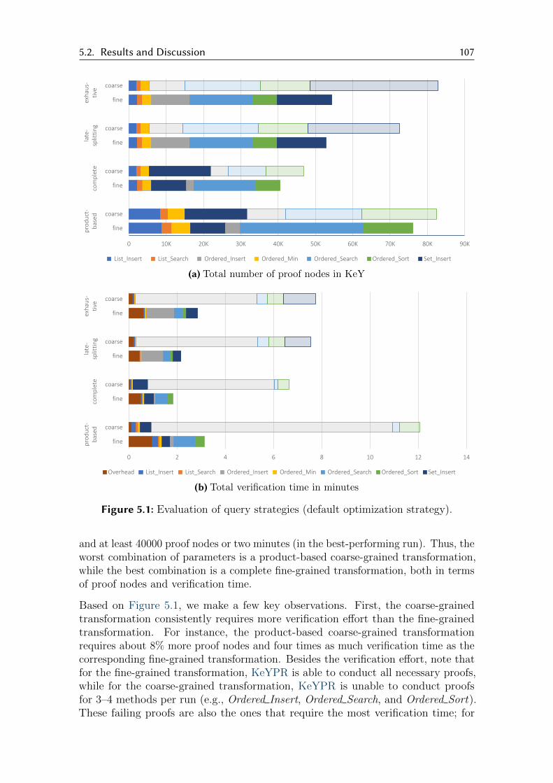
5.2. Results and Discussion 107
0 10K 20K 30K 40K 50K 60K 70K 80K 90K
fine
coarse
fine
coarse
fine
coarse
fine
coarsep
rod
uct
-b
ased
com
ple
tela
te-
split
tin
gex
hau
s-ti
ve
List_Insert List_Search Ordered_Insert Ordered_Min Ordered_Search Ordered_Sort Set_Insert
(a) Total number of proof nodes in KeY
0 2 4 6 8 10 12 14
fine
coarse
fine
coarse
fine
coarse
fine
coarse
pro
du
ct-
bas
edco
mp
lete
late
-sp
litti
ng
exh
aus-
tive
Overhead List_Insert List_Search Ordered_Insert Ordered_Min Ordered_Search Ordered_Sort Set_Insert
(b) Total verification time in minutes
Figure 5.1: Evaluation of query strategies (default optimization strategy).
and at least 40000 proof nodes or two minutes (in the best-performing run). Thus, theworst combination of parameters is a product-based coarse-grained transformation,while the best combination is a complete fine-grained transformation, both in termsof proof nodes and verification time.
Based on Figure 5.1, we make a few key observations. First, the coarse-grainedtransformation consistently requires more verification effort than the fine-grainedtransformation. For instance, the product-based coarse-grained transformationrequires about 8% more proof nodes and four times as much verification time as thecorresponding fine-grained transformation. Besides the verification effort, note thatfor the fine-grained transformation, KeYPR is able to conduct all necessary proofs,while for the coarse-grained transformation, KeYPR is unable to conduct proofsfor 3–4 methods per run (e.g., Ordered Insert, Ordered Search, and Ordered Sort).These failing proofs are also the ones that require the most verification time; for
108 5. Evaluation
instance, the failing and succeeding proofs for the product-based coarse-grainedtransformation have a verification time ratio of about 13:1. For example, the proofsfor Ordered Insert in the product-based coarse-grained transformation take aboutten minutes (five minutes twice because Ordered Insert occurs in two configurations)and, thus, 83% of the entire verification time of this run. This method is problematicin general for all coarse-grained query strategies, possibly because it contains twocalls (to original and Sort) instead of one and the contract of the Ordered Sortmethod (which the Sort call is bound to) is quite complex.
If we only compare the succeeding proofs for both transformations, we can calculatethat the fine-grained transformation, on average, requires 7% less proof nodes and8% less verification time than the coarse-grained transformation. However, whenwe also take into account the overhead time of KeYPR, we can calculate that thesucceeding proofs plus overhead of the fine-grained transformation require 17% moreverification time than the coarse-grained transformation. This is because we conductmore proofs for the fine-grained transformation (e.g., 83 proofs for the exhaustivequery strategy) than for the coarse-grained transformation (e.g., 35 proofs), andeach proof has constant overhead time for loading and saving. However, becausethis overhead is constant (cf. Section 3.4.3), we can neglect it for larger CSPLs. Insummary, we can conclude that
The coarse-grained transformation requires more verification effort than thefine-grained transformation and is less successful in conducting proofs.
Consequently, we recommend to use the fine-grained transformation for evaluatingCSPL correctness instead of the coarse-grained transformation. Recollecting ourdiscussion from Section 3.4.3, we suspect that this clear difference in verification effortis mostly due to the intermediate conditions, which cannot be leveraged as “steppingstones” by the coarse-grained transformation. We also experimented with blockcontracts and assertions in KeY [Huisman et al., 2016] to incorporate intermediateconditions in the coarse-grained transformation, but were not able to conduct theresulting proofs successfully.
Next, we compare the individual query strategies. As there are no large differencesin our data between the coarse- and fine-grained transformation when we onlyconsider the differences among our query strategies, we focus on the fine-grainedtransformation runs. Further, the data from the fine-grained transformation runs ismore reliable than the coarse-grained data because all fine-grained proofs actuallysucceed and do not trigger the stop condition. By comparison, we observe that
The query strategies require the following verification effort, ordered best toworst: complete, late-splitting, exhaustive, and product-based.
That is, the complete query strategy requires 23% less nodes and 16% less time thanthe late-splitting query strategy, which requires 3% less nodes and 24% less timethan the exhaustive query strategy, which in turn requires 29% less nodes and 9%less time than the product-based query strategy. That the complete query strategyperforms best is surprising, as this suggests that abstract contracts (as utilized by the

5.2. Results and Discussion 109
0 20K 40K 60K 80K 100K 120K
fine
coarse
fine
coarse
fine
coarsen
on
ed
efau
ltst
rict
List_Insert List_Search Ordered_Insert Ordered_Min Ordered_Search Ordered_Sort Set_Insert
(a) Total number of proof nodes in KeY
0 1 2 3 4 5 6 7 8 9
fine
coarse
fine
coarse
fine
coarse
no
ne
def
ault
stri
ct
Overhead List_Insert List_Search Ordered_Insert Ordered_Min Ordered_Search Ordered_Sort Set_Insert
(b) Total verification time in minutes
Figure 5.2: Evaluation of optimization strategies, using the exhaustive query strategy.
late-splitting and exhaustive query strategies) actually perform worse than concretecontracts (as utilized by the complete query strategy). This, however, contradictsthe potential benefits of partial proof reuse that we identified in Section 3.6.1. Wefurther discuss this in Section 5.3, where we list threats to validity regarding ourevaluation. The other findings are less surprising: First, the fine-grained late-splittingquery strategy performs slightly better (3% less nodes and 24% less time) than theexhaustive query strategy, as it identifies 9 (of 83) proofs that can safely be omitted.For the coarse-grained transformation, the late-splitting query strategy even identifies18 (of 35) omittable proofs, which is due to the larger size of connected components inthe DAGs for coarse-transformed programs (cf. Section 3.4.3). Second, the product-based query strategy performs worst of all four query strategies. This is as expected,as this query strategy is supposed to be the baseline for our evaluation.
Finally, we compare how the strict, default, and none optimization strategies influenceverification effort. To this end, we show another bar chart in Figure 5.2. In thischart, we fix the exhaustive query strategy because our optimization strategies onlyapply to the query strategies that utilize abstract contracts (i.e., exhaustive andlate-splitting). The results from this data are less clear: On the one hand, we canobserve for the coarse-grained transformation that the more we optimize, the lessproof nodes are required (strict has 29% less than default, which has 21% less than

110 5. Evaluation
none). On the other hand, verification time grows when we optimize more (by 62%from none to default and by 7% from default to strict). These results are onlypartially confirmed by the fine-grained transformation runs, however: Regardingverification time, we see a similar growth (16% from none to default and 7% fromdefault to strict), but only if we ignore the proof for Ordered Insert, which fails fornone and succeeds for default and strict. Regarding proof nodes, there are only smalldifferences between the optimization strategies when we ignore the failing proof forOrdered Insert, and a 14% reduction from none to default when we consider saidproof. To investigate further, we manually inspected the number of proof branches(i.e., points where KeY splits the proof into different cases) for the six runs shown inFigure 5.2. We found that stricter optimizations indeed corresponded with a smalleramount of branching: 2005/648 branches for none, 1078/515 for default, and 529/510for strict in the coarse-grained/fine-grained transformation. We infer that
Stricter optimization strategies tend to reduce proof nodes, but increase verifi-cation time in some cases.
Thus, we recommend to use the default optimization strategy, which served us wellfor our case study and seems to achieve a reasonable tradeoff between proof nodesand verification time. Note that no matter which optimization strategy we choose,the exhaustive query strategy cannot improve on the complete query strategy.
RQ3: Verification E�ort. After this in-depth discussion on how to choose parameterssuitably, we compare our approach for evaluating CSPL correctness with previous ap-proaches from the literature. To the best of our knowledge, there are three profoundlydifferent approaches for verifying SPLs (with several variants and combinations wedo not discuss here): First, and this is the most obvious approach, we can alwaysverify an entire SPL by verifying each product in isolation (product-based analy-ses). For large SPLs, this is infeasible; however, for small SPLs or by eliminatingredundant proofs, a product-based analysis can be acceptable. Such analyses havebeen implemented in the tools FeatureHouse [Apel et al., 2009; Benduhn, 2012;Bolle, 2017] and VarCorC [Bordis et al., 2020b; Kodetzki, 2020]. For the other twoapproaches, which both aim to reduce verification effort compared to a product-basedanalysis, there are two extreme positions we might take: Either we lift the entireSPL into the realm of the verification system (yielding a meta-product or productsimulator), so we essentially conduct one proof for the entire SPL; or we cut theSPL into many small “pieces”, which we verify separately to evaluate the correctnessafterwards. The meta-product approach corresponds to a pure family-based analysisand has been implemented by Thum et al. [2012a]. The latter approach correspondsto our feature-family-based analysis based on proof repositories and partial proofsand corresponds to the exhaustive and late-splitting query strategies in KeYPR.
To compare our analysis with previous work, we only consider approaches that allowverification of SPLs that were constructed with the CbC methodology (i.e., CSPLs).We know of only two SPL analyses that specifically take CbC into account; namelythe obvious product-based analysis as well as the optimized product-based analysisimplemented in VarCorC by Bordis et al. [2020b]. In particular, we do not know ofany meta-product approach (or purely family-based analysis in general) specificallytargeted towards CbC, which is why we omit this approach from our comparison.

5.3. Threats to Validity 111
We compare our analysis with the remaining two approaches by choosing a represen-tative run in our evaluation for each. First, we represent our feature-family-basedanalysis by the fine-grained late-splitting run, which is the best-performing run withpartial proof reuse. Second, we represent the unoptimized product-based analysis bythe fine-grained product-based run, which emulates an unoptimized product-basedanalysis as discussed in Section 3.6.2. Third, we represent the optimized product-based analysis implemented in VarCorC by the fine-grained complete run. This isbecause VarCorC also cuts the CSPL into small pieces that are verified separately(corresponding to the fine-grained transformation). Further, VarCorC does not allowfor partial proof reuse (corresponding to the complete query strategy).
Based on the data in Figure 5.1, we must then come to the conclusion that
Our feature-family-based analysis requires less verification effort than anunoptimized product-based analysis, but more verification effort than theoptimized product-based analysis implemented in VarCorC.
That is, the optimized product-based analysis requires 23% less nodes and 16% lesstime than the feature-family-based analysis, which requires 31% less nodes and 31%less time than the unoptimized product-based analysis. However, this result may beinaccurate in several ways, as we discuss below.
5.3 Threats to ValidityTo conclude, we discuss threats to the validity of our evaluation [Wohlin et al., 2012].
Internal Validity. Threats in this category mostly relate to measurement problems.First, our data in Figure 5.1 and Figure 5.2 is not averaged over several repetitions.We did perform several repetitions to design our experimental setup, but as KeYPRuses (unordered) set semantics, it was difficult to merge the evaluation results forthese repetitions. We argue, however, that this is not necessary because proof nodesare reproducible and we did not observe any noticeable differences in verificationtime across the repetitions we did perform. Second, the measurement of overheadtime is slightly off, because KeY and KeYPR use different mechanisms for measuringtime. This became apparent when we encountered a negative value for the overheadtime, which is theoretically impossible. However, we believe that this problem affectsall runs in the same way, so our arguments regarding the overhead time should bevalid nonetheless. Third, we set a stop condition for KeY that cancels a proof at alength of 10000 nodes or duration of five minutes. This makes it hard to draw anyconclusions from the lightly-colored bars in Figure 5.1 and Figure 5.2, as they canbe considered a lower bound for the verification effort of these proofs. However, weavoid the issue by focusing on the fine-grained transformation where possible, whichdoes not suffer from this problem (except for a single proof in Figure 5.2).
Construct Validity. Threats to construct validity indicate a mismatch between thetheory (i.e., Chapter 3) and construct (i.e., Chapter 4) of our evaluation. We discussone particular threat, which relates to our observation that abstract contracts performworse than concrete contracts in our evaluation. Throughout the thesis, we basically

112 5. Evaluation
assumed that a verification system with proper support for partial proofs is readily athand. However, abstract contracts as they are currently implemented in KeY do notallow for partial proof reuse, as we have observed by comparison with the completequery strategy. We believe that this is an implementation problem rather than aconceptual one, as previous evaluations of abstract contracts have shown potentialfor proof reuse [Bubel et al., 2014; Hahnle et al., 2013; Pelevina, 2014]. We identifiedtwo possible reasons why abstract contracts (and, thus, our feature-family-basedanalysis) does not perform as well as expected:
First, we make extensive use of model methods to implement our approach for contractcomposition, as model methods can be combined with abstract contracts. However,model methods also impose a high performance penalty, which we investigatedmanually on selected proofs from the complete query strategy. That is, by omittingmodel methods and performing string substitution similar to FeatureHouse instead,one proof become closable; for another proof, the number of proof nodes was halved.Possibly, this combination of model methods and abstract contracts simply does notblend well; or we introduced the problem by porting abstract contracts to KeY 2.7.
The second possible reason why abstract contracts do not perform well is moreconceptual: Pelevina [2014] notes that abstract contracts are most efficient whenemployed in complex programs with simple specifications. This is because the partialproof reuse with abstract contracts stems mostly from the symbolic execution ofcode and not from reasoning about first-order goals. However, the programs in ourevaluation have very simple code (by the nature of the fine-grained transformation,at most one statement) and complex specifications (due to contract composition),which is the precise opposite of the use case identified by Pelevina.
Thus, it is debatable whether the exhaustive and late-splitting query strategies mightperform better than the complete query strategy in a verification system with propersupport for partial proof reuse.
External Validity. Threats in this category relate to the generalizability of our findings.First, our evaluation focuses on a single case study, which is comparably small.Arguably, we could improve the external validity of our evaluation by developingmore case studies; however, this is a complex task itself and out of scope for this thesis.We argue that the size of our case study is not a problem per se, because a comparablysmall and complex codebase is realistic for applications of CbC in-field [Watson et al.,2015]. In fact, we expect that larger CSPLs only yield better results, as they havemore potential for structural and partial proof reuse. Second, our case study alsodoes not have much variability (i.e., only the method Set Insert has more than onevariant). This might be another explanation for the inefficiency of abstract contracts,as there is barely any potential for partial proof reuse in our case study. However,our justification from Section 5.2 on why we chose this particular case study stillapplies. Third, our results are only partially comparable with other implementationssuch as VarCorC and FeatureHouse. This is because KeYPR has a very specificcode generation process that has potentially big impact on verification effort. Inparticular, KeYPR cuts CbC tree in pieces and performs contract composition usingmodel methods. VarCorC, on the other hand, directly generates .problem files andthus, does not use JML or model methods at all, which hampers a direct comparison.

6. Related Work
In this thesis, we proposed a feature-family-based analysis for evaluating CSPLcorrectness that is based on the proof repository technique [Bubel et al., 2016]. Tothe best of our knowledge, our work is the first application of proof repositoriesin-field. Thus, we discuss related work that concerns CSPLs, proof reuse, and theverification of SPLs in general.
CSPLs. Pham [2017] propose an alternative approach to create CSPLs. They composePhV proof artifacts to generate products that are correct-by-construction. Thisdiffers from the approach of Bordis et al. [2020b] that we use, namely extending theCbC refinement rules themselves with support for variation. Further, Watson et al.[2016] describe a lightweight approach to reconcile the gap between CbC and PhV. Intheir approach, CbC is complemented with tools traditionally used in PhV scenariosto properly guarantee the correctness of all refinement steps. The tool CorC [Rungeet al., 2019a] is an implementation of this idea, as is our prototype KeYPR.
Proof Reuse. Steinhofel and Hahnle [2019] propose the abstract execution principle forproving properties about abstract programs, which contain abstract statements orexpressions (i.e., placeholders for concrete code). By verifying an abstract program,they can verify infinitely many concrete programs at once, which can be used, forinstance, to prove properties of program transformations (e.g., refactorings). Theirapproach has been implemented in the REFINITY workbench [Steinhofel, 2020]. Notethat abstract execution is a generalization of symbolic execution for concrete programsand also of abstract contracts [Bubel et al., 2014; Hahnle et al., 2013]. Thus, abstractexecution may be a viable alternative to abstract contracts for implementing ouranalysis. Further, as abstract execution allows abstract statements in the code, itmay allow for a generalization of our coarse-grained transformation to incompletemethods, which is infeasible with abstract contracts only.
Thum et al. [2011] introduce the proof composition approach, which uses partialproofs to reduce the verification effort of proofs in an SPL. While their goal issimilar to ours, namely achieving partial proof reuse, their notion of partial proofs isdifferent: That is, Thum et al. assign each proof step to one feature and compose

114 6. Related Work
proofs as one would compose products. In contrast, we consider proofs as black boxes(see verification states in Definition 3.14), in which we continuously bind methodcalls. Thus, our notion of partial proofs is less granular and flexible, but requires nohand-written proofs and therefore less expert knowledge in the verification system.Similarly, Klebanov [2007] proposes an approach for proof reuse that operates on aproof step level and allows for proof replay. This approach is suitable for developingand debugging a single proof, but does not address the issue of proof reuse acrossmany proofs, as required in a CSPL.
SPL Verification. Many techniques for SPL verification are known in the literature. Incontrast to our work, they focus on the PhV scenario and do not take into account theincremental nature of the CbC methodology. Thum et al. [2014a] perform a surveyand classification of such techniques, which can be grouped into product-based [Brunset al., 2010], family-based [Thum et al., 2012a], feature-product-based [Damiani et al.,2012; Thum et al., 2011], and feature-family-based [Hahnle and Schaefer, 2012]analyses. How to classify the analysis proposed in this thesis depends on the utilizedquery strategy as discussed in Section 3.6.2: The exhaustive and late-splitting querystrategies are feature-family-based analyses, while the complete and product-basedquery strategies are product-based analyses.
Note that with our proposed feature-family-based analysis, we pursue an approachthat can be considered to be opposite to family-based analyses. That is, on theone hand, family-based analyses aim to lift (or encode) the variability of an SPLinto a single meta-product, which may then be verified in one run [Apel et al., 2011,2013b; Post and Sinz, 2008; Thum et al., 2012a]. Our analysis, on the other hand,cuts the SPL into many small “pieces”, which we then verify separately. With ourapproach, the difficulty lies in identifying which pieces need to be verified (i.e., howmethod calls should be bound) and how large those pieces should be (i.e., coarse-vs. fine-grained transformation). Compared to pure family-based analyses, Thumet al. [2014a] note that feature-family-based analyses (such as ours) are better-suitedfor evolution scenarios, which usually involve only few or small changes at a time.In such a scenario, our analysis can potentially reuse many already-verified “pieces”(as mentioned in Section 3.4), while a family-based analysis either needs to re-verifythe entire meta-product or leverage reuse techniques on the verification system level(e.g., as proposed by Thum et al. [2011] and Klebanov [2007]).

7. Conclusion
The increased importance of safety-critical software systems in today’s softwareindustry necessitates new ways to guarantee software correctness. To this end, formalmethods and deductive software verification in particular can be employed. Becausesoftware is often customizable with configuration options, verification systems mustalso take variability into account and allow for the verification of entire SPLs. Verify-ing the correctness of an SPL in a post-hoc fashion, however, can be a complex taskbecause the code was not constructed with correctness in mind [Watson et al., 2016].CbC aims to solve this issue by advocating an incremental, stepwise methodology forconstructing a-priori correct programs from a given specification. It is then naturalto combine SPLs with CbC in form of CSPLs as done by Bordis et al. [2020b].
However, the potentially exponential number of products in an SPL hampers anyproduct-based analysis for evaluating CSPL correctness. In this thesis, we proposed,implemented, and evaluated a novel feature-family-based analysis for evaluatingCSPL correctness that allows for a reduction in verification effort and thereforeimproves the practical feasibility for creating CSPLs. We based our approach onproof repositories, a technique for verification-in-the-large for decoupling methodcalls from the actual called implementations [Bubel et al., 2016]. In Chapter 3,we leveraged this separation to reduce CSPLs to proof repositories, arriving at afeature-family-based analysis that allows for structural and partial proof reuse. Inaddition, our analysis (using the fine-grained transformation) is sound and complete,meaning that it can transparently replace a product-based analysis. We furtheridentified a special case of our analysis, the coarse-grained transformation, which issuitable for verifying FOP-based SPLs in a post-hoc fashion. We also discussed howour analysis may be integrated into full IDEs like VarCorC in a user-friendly manner.
In Chapter 4, we implemented our analysis in the prototype KeYPR, which can beused to interactively create CSPLs, ensuring the rule-compliance of all refinementsalong the way. KeYPR uses the verification system KeY as a backend and employsthe abstract contract mechanism for realizing partial proofs [Bubel et al., 2014;Hahnle et al., 2013]. It is possible to fully integrate KeYPR into tools like VarCorCto hide the details of the analysis from developers.
116 7. Conclusion
In Chapter 5, we evaluated our approach by creating a small case study CSPL withKeYPR and comparing our proof-repository-based analysis to previous approachesfor ensuring CSPL correctness. In the discussion of our results, we find that
• our feature-family-based analysis is feasible and can successfully be used to createand ensure the correctness of CSPLs,
• the fine-grained transformation is preferable over the coarse-grained transforma-tion for the creation of CSPLs,
• our feature-family-based analysis reduces verification effort compared to anunoptimized product-based analysis, and
• our feature-family-based analysis (at least when implemented using abstractcontracts) requires more verification effort than the optimized product-basedanalysis implemented in VarCorC.
We are optimistic that we can further accelerate our analysis in future versions ofKeYPR by revisiting the implementation of abstract contracts as discussed below,and by considering larger case studies.
Future Work. We conclude our thesis by discussing possible directions for future work.
First, we found in our evaluation that abstract contracts do not allow for the extentof partial proof reuse we had hoped for. Thus, one opportunity for future researchmight be to either improve the implementation of abstract contracts in KeY or toeven employ a different concept for partial proof reuse altogether. For instance, onepromising alternative to abstract contracts might be abstract execution [Steinhofeland Hahnle, 2019], as already discussed in Chapter 6.
Second, we only briefly discussed how to address CSPL evolution scenarios inSection 3.4.3. Evolution operators (e.g., adding and changing refinements in a CbCtree) add another dimension to the analysis, as we ideally want to achieve proof reuseover time as well. We already mentioned in Section 3.3 how this may be achievedwith “diffs” of proof repositories (or subprograms by Bubel et al.). However, toachieve proof reuse for all possible kinds of changes, more conceptual research onthis topic is needed.
Finally, we believe that there is still room for improving the proof repository tech-nique. For instance, we mentioned in Section 3.6.1 that proof repositories currentlyallow for structural and partial proof reuse inside a given method. However, proofreuse across methods (e.g., for methods with identical or very similar bodies orcontracts) is currently not supported, a restriction that future research could try tolift. Further, we showed that although the sound proof repository for a program isunique (cf. Theorem 3.2), some construction orders may be more efficient (in termsof total verification effort) than others. To take this perspective into account, ourlate-splitting heuristic proposed in Section 3.6.2 may be enhanced in future work.
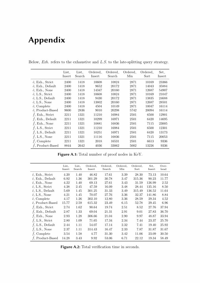
Appendix
Below, Exh. refers to the exhaustive and L.S. to the late-splitting query strategy.
ListInsert
ListSearch
OrderedInsert
OrderedSearch
OrderedMin
OrderedSort
SetInsert
c, Exh., Strict 2400 1418 10608 10824 2871 10169 23366c, Exh., Default 2400 1418 9652 20172 2871 14043 35884c, Exh., None 2400 1418 14347 20160 2871 12687 54907c, L.S., Strict 2400 1418 10608 10824 2871 10169 21047c, L.S., Default 2400 1418 9430 20172 2871 13835 24688c, L.S., None 2400 1418 13802 20160 2871 12687 28501c, Complete 2400 1418 4504 10149 2871 10047 16114c, Product-Based 9600 2836 9010 20298 5742 20094 16114
f , Exh., Strict 2211 1321 11210 16984 2501 6500 12901
f , Exh., Default 2211 1321 10299 16971 2501 6420 14695
f , Exh., None 2211 1321 10881 16836 2501 7115 23005
f , L.S., Strict 2211 1321 11210 16984 2501 6500 12301
f , L.S., Default 2211 1321 10251 16971 2501 6420 13173
f , L.S., None 2211 1321 11116 16836 2501 7115 20053
f , Complete 2211 1321 2018 16531 2501 6613 9336
f , Product-Based 8844 2642 4036 33062 5002 13226 9336
Figure A.1: Total number of proof nodes in KeY.
ListInsert
ListSearch
OrderedInsert
OrderedSearch
OrderedMin
OrderedSort
SetInsert
Over-head
c, Exh., Strict 4.20 1.40 46.82 17.61 3.39 28.30 73.13 10.64c, Exh., Default 6.92 1.36 301.29 30.78 3.47 315.36 90.23 11.77c, Exh., None 4.22 1.40 69.13 27.61 3.43 31.59 126.99 2.52c, L.S., Strict 4.38 2.45 47.59 16.09 3.48 28.44 135.16 8.50c, L.S., Default 5.69 1.45 301.25 31.33 3.49 315.49 136.52 11.64c, L.S., None 4.21 1.45 70.07 27.76 3.36 32.37 141.86 8.84c, Complete 4.17 1.26 302.10 12.80 3.36 28.59 29.34 4.52c, Product-Based 15.77 2.59 615.32 23.49 6.15 52.78 29.45 6.96
f , Exh., Strict 2.74 1.62 90.64 19.74 2.51 8.52 27.76 37.94
f , Exh., Default 2.87 1.33 69.04 21.31 2.91 9.01 27.83 36.70
f , Exh., None 2.93 1.28 306.66 21.04 2.90 9.97 48.87 33.94
f , L.S., Strict 2.80 1.09 71.65 17.34 2.34 7.44 23.37 25.70
f , L.S., Default 2.44 1.11 54.07 17.14 2.32 7.41 19.40 25.92
f , L.S., None 2.37 1.11 314.43 16.47 2.33 7.87 31.87 31.67
f , Complete 3.54 1.58 4.77 31.30 3.42 11.06 23.09 30.50
f , Product-Based 14.28 3.43 9.92 53.06 6.71 22.12 19.34 58.49
Figure A.2: Total verification time in seconds.


Bibliography
Wolfgang Ahrendt, Bernhard Beckert, Daniel Bruns, Richard Bubel, ChristophGladisch, Sarah Grebing, Reiner Hahnle, Martin Hentschel, Mihai Herda, VladimirKlebanov, Wojciech Mostowski, Christoph Scheben, Peter H. Schmitt, and MattiasUlbrich. The KeY Platform for Verification and Analysis of Java Programs. InProceedings of the Working Conference on Verified Software: Theories, Tools,and Experiments, pages 55–71. Springer, 2014. doi: 10.1007/978-3-319-12154-3 4.(cited on Page 1, 2, 6, and 97)
Wolfgang Ahrendt, Bernhard Beckert, Richard Bubel, Reiner Hahnle, Peter H.Schmitt, and Mattias Ulbrich, editors. Deductive Software Verification – The KeYBook. Springer, 2016. ISBN 9783319498126. (cited on Page 6, 7, 9, 10, 97, 104, and 105)
Sven Apel, Christian Kastner, and Christian Lengauer. FeatureHouse: Language-Independent, Automated Software Composition. In Proceedings of the InternationalConference on Software Engineering. IEEE, 2009. doi: 10.1109/icse.2009.5070523.(cited on Page 110)
Sven Apel, Hendrik Speidel, Philipp Wendler, Alexander von Rhein, and Dirk Beyer.Detection of Feature Interactions using Feature-Aware Verification. In Proceedingsof the International Conference on Automated Software Engineering, pages 372–375.IEEE, 2011. doi: 10.1109/ase.2011.6100075. (cited on Page 114)
Sven Apel, Don Batory, Christian Kastner, and Gunter Saake. Feature-OrientedSoftware Product Lines. Springer, 2013a. ISBN 9783642375217. (cited on Page 1, 5,
6, 8, and 24)
Sven Apel, Alexander von Rhein, Philipp Wendler, Armin Großlinger, and DirkBeyer. Strategies for Product-Line Verification: Case Studies and Experiments.In Proceedings of the International Conference on Software Engineering, pages482–491. IEEE, 2013b. doi: 10.1109/icse.2013.6606594. (cited on Page 2, 92, and 114)
Franz Baader and Tobias Nipkow. Term Rewriting and All That. CambridgeUniversity Press, 1998. ISBN 9781139172752. doi: 10.1017/CBO9781139172752.(cited on Page 41)
Don Batory. Feature Models, Grammars, and Propositional Formulas. In Proceedingsof the International Software Product Line Conference, pages 7–20. Springer, 2005.doi: 10.1007/11554844 3. (cited on Page 24)

120 Bibliography
Don Batory and Sean O’Malley. The Design and Implementation of HierarchicalSoftware Systems with Reusable Components. ACM Transactions on SoftwareEngineering and Methodology, 1(4):355–398, 1992. doi: 10.1145/136586.136587.(cited on Page 6 and 35)
Don Batory, Jacob Neal Sarvela, and Axel Rauschmayer. Scaling Step-Wise Re-finement. IEEE Transactions on Software Engineering, 30(6):355–371, 2004. doi:10.1109/TSE.2004.23. (cited on Page 6 and 35)
Bernhard Beckert, Reiner Hahnle, and Peter H. Schmitt, editors. Verification ofObject-Oriented Software. The KeY Approach. Springer, 2007. ISBN 9783540690610.(cited on Page 97)
Fabian Benduhn. Contract-Aware Feature Composition. Bachelor’s thesis, Otto-von-Guericke University Magdeburg, 2012. (cited on Page 110)
Gary Bernhardt. Functional Core, Imperative Shell. https://www.destroyallsoftware.com/screencasts/catalog/functional-core-imperative-shell, 2012. AccessedDecember 7, 2020. (cited on Page 100)
Yves Bertot and Pierre Casteran. Interactive Theorem Proving and Program Devel-opment. Springer, 2004. ISBN 978-3-642-05880-6. (cited on Page 6)
Stefanie Bolle. Feature-orientiertes Framing fur die Verifikation von Software-Produktlinien. Master’s thesis, Technische Universitat Braunschweig, 2017. (cited
on Page 110)
Tabea Bordis. Supporting Method Calls in CorC for Developing Correct-by-Construction Software Product Lines. Master’s thesis, Technische UniversitatBraunschweig, 2019. (cited on Page 25)
Tabea Bordis, Tobias Runge, Alexander Knuppel, Thomas Thum, and Ina Schaefer.Variational Correctness-by-Construction. In Proceedings of the InternationalWorking Conference on Variability Modelling of Software-Intensive Systems. ACM,2020a. doi: 10.1145/3377024.3377038. (cited on Page 2, 3, 14, 19, and 35)
Tabea Bordis, Tobias Runge, and Ina Schaefer. Correctness-by-Construction forFeature-Oriented Software Product Lines. In Proceedings of the InternationalConference on Generative Programming: Concepts & Experiences. ACM, 2020b.doi: 10.1145/3425898.3426959. (cited on Page 2, 3, 5, 11, 12, 17, 19, 21, 25, 35, 94, 98,
110, 113, and 115)
T. F. Bowen, F. S. Dworack, C. H. Chow, N. Griffeth, G. E. Herman, and Y.-J. Lin.The Feature Interaction Problem in Telecommunications Systems. In InternationalConference on Software Engineering for Telecommunication Switching Systems,pages 59–62. IET, 1989. (cited on Page 91)
Daniel Bruns, Vladimir Klebanov, and Ina Schaefer. Verification of Software ProductLines with Delta-Oriented Slicing. In Proceedings of the International Conferenceon Formal Verification of Object-Oriented Software, pages 61–75. Springer, 2010.doi: 10.1007/978-3-642-18070-5 5. (cited on Page 114)

Bibliography 121
Richard Bubel, Reiner Hahnle, and Maria Pelevina. Fully Abstract OperationContracts. In Tiziana Margaria and Bernhard Steffen, editors, Proceedings ofthe International Symposium On Leveraging Applications of Formal Methods,Verification and Validation, pages 120–134. Springer, 2014. doi: 10.1007/978-3-662-45231-8 9. (cited on Page 2, 36, 97, 112, 113, and 115)
Richard Bubel, Ferruccio Damiani, Reiner Hahnle, Einar Broch Johnsen, OlafOwe, Ina Schaefer, and Ingrid Chieh Yu. Proof Repositories for CompositionalVerification of Evolving Software Systems. In Bernhard Steffen, editor, Transactionson Foundations for Mastering Change I, pages 130–156. Springer, 2016. doi:10.1007/978-3-319-46508-1 8. (cited on Page 2, 3, 10, 11, 17, 36, 37, 40, 42, 48, 50, 88, 93,
94, 97, 113, 115, and 116)
Gunter Bockle, Peter Knauber, Klaus Pohl, and Klaus Schmid. Software-Produktlinien: Methoden, Einfuhrung und Praxis. dpunkt-Verlag, 2004. ISBN978-3-89864-257-6. (cited on Page 5)
Paul Clements and Linda Northrop. Software Product Lines: Practices and Patterns.Addison-Wesley, 2002. ISBN 9780201703320. (cited on Page 1 and 5)
Alistair Cockburn. Hexagonal Architecture. http://web.archive.org/web/20201101022836/https://alistair.cockburn.us/hexagonal-architecture/, 2005. AccessedDecember 7, 2020. (cited on Page 100)
Edgar F. Codd. A Relational Model of Data for Large Shared Data Banks. Com-munications of the ACM, 13(6):377–387, 1970. doi: 10.1007/978-3-642-48354-7 4.(cited on Page 22)
Ferruccio Damiani, Johan Dovland, Einar Broch Johnsen, Olaf Owe, Ina Schaefer,and Ingrid Chieh Yu. A Transformational Proof System for Delta-Oriented Pro-gramming. In Proceedings of the International Software Product Line Conference,pages 53–60. ACM, 2012. doi: 10.1145/2364412.2364422. (cited on Page 114)
Stijn de Gouw, Jurriaan Rot, Frank S. de Boer, Richard Bubel, and Reiner Hahnle.OpenJDK’s Java.utils.Collection.sort() Is Broken: The Good, the Bad and theWorst Case. In Proceedings of the International Conference on Computer AidedVerification, pages 273–289. Springer, 2015. doi: 10.1007/978-3-319-21690-4 16.(cited on Page 1)
Edsger W. Dijkstra. A Constructive Approach to the Problem of Program Correctness.BIT Numerical Mathematics, 8(3):174–186, 1968. doi: 10.1007/bf01933419. (cited
on Page 12)
Edsger W. Dijkstra. Guarded Commands, Nondeterminacy and Formal Derivationof Programs. Communications of the ACM, 18(8):453–457, 1975. doi: 10.1145/360933.360975. (cited on Page 12 and 20)
Edsger W. Dijkstra. A Discipline of Programming. Prentice Hall, 1976. ISBN978-0132158718. (cited on Page 1 and 6)
122 Bibliography
David S. Dummit and Richard M. Foote. Abstract Algebra. Wiley, 2003. ISBN978-0-471-43334-7. (cited on Page 49 and 84)
Christian Engel, Andreas Roth, Peter H. Schmitt, and Benjamin Weiß. Verificationof Modifies Clauses in Dynamic Logic with Non-rigid Functions. Research report 9,Universitat Karlsruhe, 2009. (cited on Page 6, 24, and 41)
Shannon Fischer, Lukas Linsbauer, Roberto E. Lopez-Herrejon, and AlexanderEgyed. Enhancing Clone-and-Own with Systematic Reuse for Developing SoftwareVariants. In Proceedings of the International Conference on Software Maintenanceand Evolution, pages 391–400. IEEE, 2014. doi: 10.1109/ICSME.2014.61. (cited on
Page 1)
Robert W. Floyd. Assigning Meanings to Programs. In Timothy R. Colburn, James H.Fetzer, and Terry L. Rankin, editors, Program Verification, pages 65–81. Springer,1993. doi: 10.1007/978-94-011-1793-7 4. (cited on Page 6 and 13)
David Gries. The Science of Programming. Springer, 1981. ISBN 3540964800. (cited
on Page 1 and 6)
Anthony Hall and Roderick Chapman. Correctness by Construction: Developing aCommercial Secure System. IEEE Software, 19(1):18–25, 2002. doi: 10.1109/52.976937. (cited on Page 12)
David Harel. First-Order Dynamic Logic. Springer, 1979. ISBN 3-540-09237-4. doi:10.1007/3-540-09237-4. (cited on Page 9)
Richard Helm, Ian M. Holland, and Dipayan Gangopadhyay. Contracts: SpecifyingBehavioral Compositions in Object-Oriented Systems. ACM SIGPLAN Notices,25(10):169–180, 1990. doi: 10.1145/97946.97967. (cited on Page 6)
Rich Hickey. The Clojure Programming Language. In Proceedings of the Symposiumon Dynamic Languages. ACM, 2008. doi: 10.1145/1408681.1408682. (cited on
Page 98)
C. A. R. Hoare. An Axiomatic Basis for Computer Programming. Communicationsof the ACM, 12(10):576–580, 1969. doi: 10.1145/363235.363259. (cited on Page 6
and 13)
Marieke Huisman, Wolfgang Ahrendt, Daniel Grahl, and Martin Hentschel. FormalSpecification with the Java Modeling Language. In Wolfgang Ahrendt, BernhardBeckert, Richard Bubel, Reiner Hahnle, Peter H. Schmitt, and Mattias Ulbrich,editors, Deductive Software Verification – The KeY Book, chapter 7, pages 193–241.Springer, 2016. doi: 10.1007/978-3-319-49812-6 7. (cited on Page 100 and 108)
Reiner Hahnle and Ina Schaefer. A Liskov Principle for Delta-Oriented Programming.In Proceedings of the International Symposium On Leveraging Applications ofFormal Methods, Verification and Validation, pages 32–46. Springer, 2012. doi:10.1007/978-3-642-34026-0 4. (cited on Page 114)

Bibliography 123
Reiner Hahnle, Ina Schaefer, and Richard Bubel. Reuse in Software Verificationby Abstract Method Calls. In Proceedings of the International Conference onAutomated Deduction, pages 300–314. Springer, 2013. doi: 10.1007/978-3-642-38574-2 21. (cited on Page 2, 36, 97, 112, 113, and 115)
IEEE. Systems and Software Engineering–Vocabulary. International Standard24765:2017(E), ISO/IEC/IEEE, 2017. (cited on Page 14 and 15)
Jean-Marc Jezequel and Betrand Meyer. Design by Contract: The Lessons of Ariane.IEEE Computer, 30(1):129–130, 1997. doi: 10.1109/2.562936. (cited on Page 1)
Kyo C. Kang, Sholom G. Cohen, James A. Hess, William E. Novak, and A. SpencerPeterson. Feature-Oriented Domain Analysis (FODA) Feasibility Study. TechnicalReport CMU/SEI-90-TR-21, Software Engineering Institute, Carnegie MellonUniversity, 1990. (cited on Page 5 and 24)
Vladimir Klebanov. Proof Reuse. In Bernhard Beckert, Reiner Hahnle, and Peter H.Schmitt, editors, Verification of Object-Oriented Software. The KeY Approach,pages 507–529. Springer, 2007. doi: 10.1007/978-3-540-69061-0 13. (cited on Page 88
and 114)
Peter Knauber, Jesus Bermejo Munoz, Gunter Bockle, Julio Cesar Sampaio do PradoLeite, Frank van der Linden, Linda Northrop, Michael Stark, and David M. Weiss.Quantifying Product Line Benefits. In Proceedings of the International Workshopon Software Product-Family Engineering, pages 155–163. Springer, 2001. doi:10.1007/3-540-47833-7 15. (cited on Page 1 and 5)
Alexander Knuppel, Thomas Thum, Carsten Padylla, and Ina Schaefer. Scalabilityof Deductive Verification Depends on Method Call Treatment. In Proceedingsof the International Symposium On Leveraging Applications of Formal Methods,Verification and Validation, pages 159–175. Springer, 2018. doi: 10.1007/978-3-030-03427-6 15. (cited on Page 10 and 104)
Maximilian Kodetzki. Variational Correctness-by-Construction fur Software-Produktlinien mit FeatureIDE. Bachelor’s thesis, Technische Universitat Braun-schweig, 2020. (cited on Page 25, 98, and 110)
Derrick G. Kourie and Bruce W. Watson. The Correctness-by-Construction Approachto Programming. Springer, 2012. ISBN 978-3-642-27918-8. doi: 10.1007/978-3-642-27919-5. (cited on Page 1, 12, 16, 17, 20, 25, 26, and 105)
Charles W. Krueger. New Methods in Software Product Line Development. InProceedings of the International Software Product Line Conference. IEEE, 2006.doi: 10.1109/spline.2006.1691581. (cited on Page 2)
Joseph B. Kruskal, Jr. On the Shortest Spanning Subtree of a Graph and theTraveling Salesman Problem. Proceedings of the American Mathematical Society,7(1):48–48, 1956. doi: 10.1090/s0002-9939-1956-0078686-7. (cited on Page 47)
Gary T. Leavens and Yoonsik Cheon. Design by Contract with JML. Technicalreport, 2006. (cited on Page 6 and 37)

124 Bibliography
Gary T. Leavens, Albert L. Baker, and Clyde Ruby. JML: a Java Modeling Language.Technical report, 1998. (cited on Page 6 and 37)
Barbara H. Liskov and Jeannette M. Wing. A Behavioral Notion of Subtyping. ACMTransactions on Programming Languages and Systems, 16(6):1811–1841, 1994. doi:10.1145/197320.197383. (cited on Page 2 and 27)
Jing Liu, Josh Dehlinger, and Robyn Lutz. Safety Analysis of Software ProductLines using State-Based Modeling. In Proceedings of the International Symposiumon Software Reliability Engineering, pages 10–30. IEEE, 2007. doi: 10.1109/issre.2005.36. (cited on Page 1)
Roberto E. Lopez-Herrejon and Don Batory. A Standard Problem for EvaluatingProduct-Line Methodologies. In Proceedings of the International Conference onGenerative and Component-Based Software Engineering, pages 10–24. Springer,2001. doi: 10.1007/3-540-44800-4 2. (cited on Page 25)
Saunders Mac Lane. Categories for the Working Mathematician. Springer, 1978.ISBN 978-1-4419-3123-8. (cited on Page 46)
M. Douglas McIlroy. Macro Instruction Extensions of Compiler Languages. Commu-nications of the ACM, 3(4):214–220, 1960. doi: 10.1145/367177.367223. (cited on
Page 98)
Marcilio Mendonca, Andrzej W ↪asowski, and Krzysztof Czarnecki. SAT-Based Analysisof Feature Models is Easy. In Proceedings of the International Software ProductLine Conference, pages 231–240. ACM, 2009. (cited on Page 24)
Bertrand Meyer. Applying “Design by Contract”. IEEE Computer, 25(10):40–51,1992. doi: 10.1109/2.161279. (cited on Page 6 and 12)
Maria Pelevina. Realization and Extension of Abstract Operation Contracts forProgram Logic. Bachelor’s thesis, Technische Universitat Darmstadt, 2014. (cited
on Page 2, 97, 101, and 112)
Thi-Kim-Dung Pham. Development of Correct-by-Construction Software usingProduct Lines. PhD thesis, CNAM Paris, 2017. (cited on Page 113)
Klaus Pohl, Gunter Bockle, and Frank van der Linden. Software Product LineEngineering: Foundations, Principles and Techniques. Springer, 2005. ISBN9783540243724. (cited on Page 1 and 5)
Emil L. Post. Recursively Enumerable Sets of Positive Integers and Their DecisionProblems. Bulletin of the American Mathematical Society, 50:284–316, 1944. doi:10.1090/S0002-9904-1944-08111-1. (cited on Page 71 and 85)
Hendrik Post and Carsten Sinz. Configuration Lifting: Verification meets SoftwareConfiguration. In Proceedings of the International Conference on AutomatedSoftware Engineering, pages 347–350. IEEE, 2008. doi: 10.1109/ase.2008.45. (cited
on Page 2 and 114)

Bibliography 125
Trygve Reenskaug, Egil P. Andersen, Arne Jorgen Berre, Anne Hurlen, AntonLandmark, Odd Arild Lehne, Else Nordhagen, Eirik Ness-Ulseth, Gro Oftedal,Anne Lise Skaar, and Pal Stenslet. OORASS: Seamless Support for the Creation andMaintenance of Object-Oriented Systems. Journal of Object-Oriented Programming,5(6):27–41, 1992. (cited on Page 25)
Tobias Runge, Ina Schaefer, Loek Cleophas, Thomas Thum, Derrick Kourie, andBruce W. Watson. Tool Support for Correctness-by-Construction. In Proceedings ofthe International Conference on Fundamental Approaches to Software Engineering,pages 25–42. Springer, 2019a. doi: 10.1007/978-3-030-16722-6 2. (cited on Page 2,
7, 14, 15, 75, 97, and 113)
Tobias Runge, Thomas Thum, Loek Cleophas, Ina Schaefer, and Bruce W. Watson.Comparing Correctness-by-Construction with Post-Hoc Verification—A QualitativeUser Study. In Proceedings of the International Symposium on Formal Methods,pages 388–405. Springer, 2019b. doi: 10.1007/978-3-030-54997-8 25. (cited on
Page 98 and 106)
Ina Schaefer, Lorenzo Bettini, Viviana Bono, Ferruccio Damiani, and Nico Tanzarella.Delta-Oriented Programming of Software Product Lines. In Proceedings of theInternational Software Product Line Conference, pages 77–91. Springer, 2010. doi:10.1007/978-3-642-15579-6 6. (cited on Page 2)
Pierre-Yves Schobbens, Patrick Heymans, and Jean-Christophe Trigaux. FeatureDiagrams: A Survey and a Formal Semantics. In Proceedings of the InternationalConference on Requirements Engineering, pages 139–148. IEEE, 2006. doi: 10.1109/RE.2006.23. (cited on Page 35)
Wolfgang Scholz, Thomas Thum, Sven Apel, and Christian Lengauer. AutomaticDetection of Feature Interactions using the Java Modeling Language. In Proceedingsof the International Software Product Line Conference. ACM, 2011. doi: 10.1145/2019136.2019144. (cited on Page 25)
Yannis Smaragdakis and Don Batory. Mixin Layers: An Object-Oriented Imple-mentation Technique for Refinements and Collaboration-Based Designs. ACMTransactions on Software Engineering and Methodology, 11(2):215–255, 2002. doi:10.1145/505145.505148. (cited on Page 6 and 25)
Dominic Steinhofel. REFINITY to Model and Prove Program Transformation Rules.In Asian Symposium on Programming Languages and Systems, pages 311–319.Springer, 2020. doi: 10.1007/978-3-030-64437-6 16. (cited on Page 113)
Dominic Steinhofel and Reiner Hahnle. Abstract Execution. In Proceedings of theInternational Symposium on Formal Methods, pages 319–336. Springer, 2019. doi:10.1007/978-3-030-30942-8 20. (cited on Page 113 and 116)
Maurice H. ter Beek, Reiner Hahnle, and Ina Schaefer. Correctness-by-Constructionand Post-hoc Verification: Friends or Foes? In Proceedings of the InternationalSymposium On Leveraging Applications of Formal Methods, Verification andValidation, pages 723–729. Springer, 2016. doi: 10.1007/978-3-319-47166-2 51.(cited on Page 16)

126 Bibliography
Thomas Thum, Don Batory, and Christian Kastner. Reasoning About Edits toFeature Models. In Proceedings of the International Conference on SoftwareEngineering, pages 254–264. IEEE, 2009. doi: 10.1109/ICSE.2009.5070526. (cited
on Page 35)
Thomas Thum, Ina Schaefer, Martin Kuhlemann, and Sven Apel. Proof Composi-tion for Deductive Verification of Software Product Lines. In Proceedings of theInternational Conference on Software Testing, Verification and Validation, pages270–277. IEEE, 2011. doi: 10.1109/icstw.2011.48. (cited on Page 37, 113, and 114)
Thomas Thum, Ina Schaefer, Sven Apel, and Martin Hentschel. Family-Based De-ductive Verification of Software Product Lines. In Proceedings of the InternationalConference on Generative Programming: Concepts & Experiences, pages 11–20.ACM, 2012a. doi: 10.1145/2371401.2371404. (cited on Page 37, 110, and 114)
Thomas Thum, Ina Schaefer, Martin Kuhlemann, Sven Apel, and Gunter Saake.Applying Design by Contract to Feature-Oriented Programming. In Proceedings ofthe International Conference on Fundamental Approaches to Software Engineering,pages 255–269. Springer, 2012b. doi: 10.1007/978-3-642-28872-2 18. (cited on
Page 75)
Thomas Thum, Sven Apel, Christian Kastner, Ina Schaefer, and Gunter Saake. AClassification and Survey of Analysis Strategies for Software Product Lines. ACMComputing Surveys, 47(1):1–45, 2014a. doi: 10.1145/2580950. (cited on Page 2, 35,
88, 90, 92, and 114)
Thomas Thum, Jens Meinicke, Fabian Benduhn, Martin Hentschel, Alexander vonRhein, and Gunter Saake. Potential Synergies of Theorem Proving and ModelChecking for Software Product Lines. In Proceedings of the International SoftwareProduct Line Conference, pages 177–186. ACM, 2014b. doi: 10.1145/2648511.2648530. (cited on Page 37)
Thomas Thum, Alexander Knuppel, Stefan Kruger, Stefanie Bolle, and Ina Schaefer.Feature-Oriented Contract Composition. Journal of Systems and Software, 152:83–107, 2019. doi: 10.1016/j.jss.2019.01.044. (cited on Page 1, 2, 27, 29, and 35)
Bruce W. Watson, Derrick G. Kourie, and Loek Cleophas. Experience withCorrectness-by-Construction. Science of Computer Programming, 97:55–58, 2015.doi: 10.1016/j.scico.2013.11.024. (cited on Page 112)
Bruce W. Watson, Derrick G. Kourie, Ina Schaefer, and Loek Cleophas. Correctness-by-Construction and Post-hoc Verification: A Marriage of Convenience? InProceedings of the International Symposium On Leveraging Applications of FormalMethods, Verification and Validation, pages 730–748. Springer, 2016. doi: 10.1007/978-3-319-47166-2 52. (cited on Page 7, 10, 16, 75, 105, 113, and 115)
Claes Wohlin, Per Runeson, Martin Host, Magnus C. Ohlsson, and Bjorn Regnell.Experimentation in Software Engineering. Springer, 2012. ISBN 9783642290435.(cited on Page 111)

I herewith assure that I wrote the present thesis independently, that the thesis hasnot been partially or fully submitted as graded academic work and that I have usedno other means than the ones indicated. I have indicated all parts of the work inwhich sources are used according to their wording or to their meaning.
Magdeburg, 24th December 2020