projet de fin d’etudes - insa...
TRANSCRIPT

Ecole Nationale Superieure de Physique de Strasbourg INSA de Strasbourg
Integration of a Pan-Tilt-Zoom camera in a multiRGB+D sensor system in order to get high
resolution data for behavior analysis of children andperform real-time tracking
Projet de Fin d’Etudes
Specialite Mecatronique
September 2012Arnaud Bruyas
Department of Computer Science and Engineering,Center of Distributed Robotics, University of Minnesota

INSA - ENSPS Arnaud Bruyas University of Minnesota
Abstract
This document was written in the scope of an internship for the National Superior Physics Schoolof Strasbourg (ENSPS) and the National Institut of Applied Sciences (INSA) of Strasbourg. This fivemonths project occurred in the Center for Distributed Robotics of the University of Minnesota, underthe supervision of Nikos Papanikolopoulos, professor at the University and director of the laboratory.This document has been writen to present the work achieved during the internship and to describethe results of the carried out research. The goal of the main project this internship is part of is,the monitoring of children and the detection of possible at-risk markers of mental illnesses using non-intrusive sensors in a lab-school (see appendix F). After introducing the context of the internship andpresenting the main project, this paper is focused on the subject of my project, and highlights somerelated projects and algorithms that act as a basis for the work. Then the work that had been achievedduring this period is explained, by presenting the implemented algorithms and analyzing the results.
The first part of the project had consisted in designing a software to control a PTZ camera alreadyavailable in the lab, and ensure the feasibility of a real-time tracking using this device. Then wedeveloped a simple tracking algorithm, using covariance descriptors as a way of representing objects.In the end, despite the low quality of the actual camera hardware, it appears that a real-time trackingis feasible, but highly related to the features used in the descriptor. So keeping in mind the real-timeobjective, an optimization algorithm has been performed over the descriptor composition. To solve thisMultiple Objectives Combinatorial problem, a Genetic Algorithm has been set up, using the trackingalgorithm described before as a black box which gives the performances of a descriptor. In the end,different tests had been run over several videos in order to observe the behaviour of the GA. Theresults are consistent but due to the nature of the GA, nothing ensure that the best combination hasbeen found.
Resume
Ce document a ete redige dans le cadre d’un stagee pour le compte de l’Ecole Nationale Superieure dePhysique de Strasbourg (ENSPS) et l’Institut National des Sciences appliquees (INSA) de Strasbourg.D’une duree de 5 mois, ce projet a ete realise au sein du departement d’Ingenierie Informatique etRobotique (Center for Distributed Robotics) de l’Universite du Minnesota, sous la tutel de MonsieurNikos Papanikolopoulos, professeur au sein de l’Univeriste. Ce document a ete redige dans le but depresenter le travail effectue et les resultats des recherches menees au cours du stage. Le projet presentedans ce document s’inscrit dans un projet plus large, qui a pour but l’observation d’enfants en bas-agel’aide de cameras, pour detecter de possibles signes de problemes mentaux (voir annexe F). Apresune description du contexte et du sujet du stage, ce document introduit quelques travaux similairesdont certains elements ont ete utilises au cours du projet. Ensuite, le travail realise durant le stage estdetaille et les differents outils utilises sont expliques.
La premiere partie du stage a ete consacree a la creation d’un programme informatique pourcontroler une PTZ camera, et s’assurer de la faisabilite d’un tracking en temps reel. Dans la suitedu projet, un programme a ete developpe pour le tracking, en utilisant des descripteurs bases surla covariance (covariance descriptors). Cependant, la rapidite de l’algorithme est fortement liee auxcaracteristiques de ce descripteur. Donc en gardant a l’esprit la contrainte temps reel, un AlgorithmGenetique a ete mis au point afin d’optimiser la composition des descripteurs en fonction de l’objetsuivi. Cet AG utilise l’algorithme de suivi developpe auparavant comme une boite noire. Les perfor-mances a optimiser sont la precision et la rapidite d’execution du suivi. Les resultats presentes a la finsemblent coherents, mais rien n’assure que le meilleur descripteur a ete trouve.
1

INSA - ENSPS Arnaud Bruyas University of Minnesota
Acknoledgments
I first want to thank Professor Nikos Papanikolopoulos, for accepting me in his laboratory during thisinternship, and trusting my abilities for researches. This internship would not have happen withouthim. He also let me conduct my own work about something I like, which is a proof of trust that Iappreciate. He also offered the opportunity to attend to ICRA 2012 and discover all the state of theart projects that are leaded in the robotic field nowadays.
I also want to give thanks to Josh, Nick and Bill, who are currently working on the project. Theyhelped me a lot all along the internship when I had difficulties or when I needed new ideas to solve aproblem. Their help and their knowledge in the programming field had been very helpful.
My thanks also go to all the people in the lab, for giving me a warm welcome and show me allthe amazing projects they are working on. I especially thank Duc, for showing me the University andthe lab in the beginning. I really appreciate to have someone nearby with who it was possible to talkFrench to.
I also acknowledge Mrs Cecilia Zanni-Merk, for reading all my weekly reports and giving me usefuladvices all along the project.
I also give thanks to Professor Jacque Gangloff, for giving me the opportunity to contact MrPapanikolopoulos. This great experience wouldn’t have been possible without him.
2

INSA - ENSPS Arnaud Bruyas University of Minnesota
Introduction
As part of my education plan at the National Institute of Applied Sciences (INSA) of Strasbourgand in order to get my engineer degree, I have to carry out a five months internship in a professionalinstitution. But I also took the opportunity offered to get a Master in partnership with the NationalSuperior Physics School of Strasbourg (ENSPS). This master was for me the opportunity to focus mystudies on the robotic and vision field, but also to discover the research area. Since USA is at thestate of the art in Computer Vision, I decided to search an internship in an American laboratory. Ihad the opportunity to be in contact with Nikos Papanikolopoulos, who is professor at the Universityof Minnesota, but also director of the Center of Distributed Robotics in this University. He agreed toreceive me in his laboratory and gave me the possibility to be part of a project at the cutting-edge ofthe Vision field. It concerns the monitoring of toddlers in order to detect possible at-risk markers thatcould highlight mental illnesses. For this purpose, the system is using several Kinect sensors in orderto be able to reconstruct a full 3D representation of the scene.
This document presents the project I worked on, by first introducing some helpful related work.Then the work carried out and the experiments run are explained. Finally, the results are exposedand some conclusions are made.
3

INSA - ENSPS Arnaud Bruyas University of Minnesota
Contents
I Presentation of the project and Definition of the problem 7
1 Current system presentation 71.1 Achievements . . . . . . . . . . . . . . . . . . . . . . . . . . . . . . . . . . . . . . . . . . 7
1.1.1 Calibration . . . . . . . . . . . . . . . . . . . . . . . . . . . . . . . . . . . . . . . 71.1.2 Methodology . . . . . . . . . . . . . . . . . . . . . . . . . . . . . . . . . . . . . . 71.1.3 Behavior analysis and results . . . . . . . . . . . . . . . . . . . . . . . . . . . . . 9
2 Definition and description of my work in the project 92.1 Definition of the subject . . . . . . . . . . . . . . . . . . . . . . . . . . . . . . . . . . . . 92.2 Related and similar projects . . . . . . . . . . . . . . . . . . . . . . . . . . . . . . . . . . 10
II Related Work 11
3 Project key points and related works 113.1 Master/Slave relation . . . . . . . . . . . . . . . . . . . . . . . . . . . . . . . . . . . . . 113.2 Calibration . . . . . . . . . . . . . . . . . . . . . . . . . . . . . . . . . . . . . . . . . . . 11
3.2.1 Camera model . . . . . . . . . . . . . . . . . . . . . . . . . . . . . . . . . . . . . 113.2.2 Intrinsic parameters . . . . . . . . . . . . . . . . . . . . . . . . . . . . . . . . . . 113.2.3 Extrinsic parameters . . . . . . . . . . . . . . . . . . . . . . . . . . . . . . . . . . 12
3.3 PTZ camera servoing . . . . . . . . . . . . . . . . . . . . . . . . . . . . . . . . . . . . . . 123.3.1 Pan-tilt control . . . . . . . . . . . . . . . . . . . . . . . . . . . . . . . . . . . . . 123.3.2 Zoom control . . . . . . . . . . . . . . . . . . . . . . . . . . . . . . . . . . . . . . 13
3.4 Target detection . . . . . . . . . . . . . . . . . . . . . . . . . . . . . . . . . . . . . . . . 133.4.1 Skin color detection . . . . . . . . . . . . . . . . . . . . . . . . . . . . . . . . . . 133.4.2 Movement detection . . . . . . . . . . . . . . . . . . . . . . . . . . . . . . . . . . 143.4.3 Covariance descriptors . . . . . . . . . . . . . . . . . . . . . . . . . . . . . . . . . 14
3.5 Optimization of the descriptors composition . . . . . . . . . . . . . . . . . . . . . . . . . 153.5.1 A Simulated Annealing method . . . . . . . . . . . . . . . . . . . . . . . . . . . . 153.5.2 A Genetic Algorithm . . . . . . . . . . . . . . . . . . . . . . . . . . . . . . . . . . 15
III Planning of the project 183.6 Considered work . . . . . . . . . . . . . . . . . . . . . . . . . . . . . . . . . . . . . . . . 183.7 Time schedule . . . . . . . . . . . . . . . . . . . . . . . . . . . . . . . . . . . . . . . . . . 18
IV Achieved Work, Results and Comments 19
4 Camera Setup and Control 194.1 Camera Specifications . . . . . . . . . . . . . . . . . . . . . . . . . . . . . . . . . . . . . 194.2 Camera Control . . . . . . . . . . . . . . . . . . . . . . . . . . . . . . . . . . . . . . . . . 204.3 Movements Calculation . . . . . . . . . . . . . . . . . . . . . . . . . . . . . . . . . . . . 23
5 Tracking Task 245.1 Computation of the Covariance Descriptor . . . . . . . . . . . . . . . . . . . . . . . . . . 245.2 Tracking Algorithm . . . . . . . . . . . . . . . . . . . . . . . . . . . . . . . . . . . . . . . 245.3 C++ Implementation . . . . . . . . . . . . . . . . . . . . . . . . . . . . . . . . . . . . . 245.4 Toward a real time tracking . . . . . . . . . . . . . . . . . . . . . . . . . . . . . . . . . . 24
4

INSA - ENSPS Arnaud Bruyas University of Minnesota
6 Optimization of the Descriptor’s composition 266.1 Definition of the Problem and creation of the ground truth . . . . . . . . . . . . . . . . 266.2 Creation of chromosomes as a good way to represent the descriptors . . . . . . . . . . . 276.3 Description of the steps of the GA . . . . . . . . . . . . . . . . . . . . . . . . . . . . . . 29
6.3.1 Initialisation . . . . . . . . . . . . . . . . . . . . . . . . . . . . . . . . . . . . . . 296.3.2 Selection and Reproduction . . . . . . . . . . . . . . . . . . . . . . . . . . . . . . 296.3.3 Termination Criterion . . . . . . . . . . . . . . . . . . . . . . . . . . . . . . . . . 30
6.4 C++ Implementation . . . . . . . . . . . . . . . . . . . . . . . . . . . . . . . . . . . . . 306.5 First Tests . . . . . . . . . . . . . . . . . . . . . . . . . . . . . . . . . . . . . . . . . . . . 33
6.5.1 Setup of the Experiment . . . . . . . . . . . . . . . . . . . . . . . . . . . . . . . . 336.5.2 Results . . . . . . . . . . . . . . . . . . . . . . . . . . . . . . . . . . . . . . . . . 346.5.3 Comments and chromosome composition . . . . . . . . . . . . . . . . . . . . . . . 35
6.6 Tests on real video set recorded in the Lab School . . . . . . . . . . . . . . . . . . . . . 386.6.1 Description of the Experiment . . . . . . . . . . . . . . . . . . . . . . . . . . . . 386.6.2 Results and Comments for the first video sequence . . . . . . . . . . . . . . . . . 396.6.3 Results and Comments for the second video sequence . . . . . . . . . . . . . . . 41
6.7 Conclusion on the GA performances . . . . . . . . . . . . . . . . . . . . . . . . . . . . . 41
V Conclusion 43
VI Appendices 44
A Evolution of the chromosome set using the first selection method on the coffee boxvideo 45
B Evolution of the chromosome set using the second selection method on the coffeebox video 49
C Details of several tests run using the new termination criterion 53
D Different set of chromosomes on the first video recorded at the lab-school, usingthe first selection method 55
E Different set of chromosomes on the first video recorded at the lab-school, usingthe second selection method 59
F New Scientist article about the project 63
G Description of the Center of Distributed Robotics 65
H Working in a laboratory of an American University 66
I ICRA 2012 in Saint Paul - Minneapolis: A unique experience 67
J ICRA paper 68
5

INSA - ENSPS Arnaud Bruyas University of Minnesota
List of Figures
1 Methodology (extracted from [3]) . . . . . . . . . . . . . . . . . . . . . . . . . . . . . . . 82 Time schedule for the project . . . . . . . . . . . . . . . . . . . . . . . . . . . . . . . . . 183 Size of the same square in the image for different zoom steps . . . . . . . . . . . . . . . 204 Size of the same square in different images after zoom in and a zoom out commands . . 215 Size of the same square in different images after zooming in 6x and a zooming out 3
times 2x . . . . . . . . . . . . . . . . . . . . . . . . . . . . . . . . . . . . . . . . . . . . . 216 Simulation of the preset positions method . . . . . . . . . . . . . . . . . . . . . . . . . . 227 Focal lenght on the X and Y axis depending on the zoom position . . . . . . . . . . . . 238 Graphic presenting the real positions (red) and the estimated positions using a linear
estimation (blue) . . . . . . . . . . . . . . . . . . . . . . . . . . . . . . . . . . . . . . . . 259 Graphic presenting the real positions (red) and the estimated positions using a polyno-
mial estimation (blue) . . . . . . . . . . . . . . . . . . . . . . . . . . . . . . . . . . . . . 2510 Graphic presenting the real positions (red) and the estimated positions (blue) . . . . . . 2811 Comparaison of the real and the estimated points over the time . . . . . . . . . . . . . . 2812 Diagram of the process for the creation of a chromosome . . . . . . . . . . . . . . . . . . 2913 Graphic of the different elements of the quality interpretation . . . . . . . . . . . . . . . 3114 Example of the display and the corresponding report . . . . . . . . . . . . . . . . . . . . 3215 Initial frame of the coffee box video, with a bounding box around the tracked object . . 3316 Diagram of the final set of chromosome using the first method . . . . . . . . . . . . . . . 3417 Diagram of the final set of chromosome using the second method . . . . . . . . . . . . . 3518 Diagram of the final set of chromosome using the second method and the tremination
criterion . . . . . . . . . . . . . . . . . . . . . . . . . . . . . . . . . . . . . . . . . . . . . 3619 Initial set of chromosomes using the first Selection method with 60 chromosomes . . . . 3620 Final set of chromosomes using the first Selection method with 60 chromosomes . . . . . 3621 Initial set of chromosomes using the second Selection method with 60 chromosomes . . . 3722 Final set of chromosomes using the second Selection method with 60 chromosomes . . . 3723 Initial frame of the first video sequence, with a bounding box on the target . . . . . . . 3824 Initial frame of the second video sequence, with a bounding box on the target . . . . . . 3825 Representation of the final chromosome set in the NOS, using the Selection/Reproduction
method 1 on a Real Data video . . . . . . . . . . . . . . . . . . . . . . . . . . . . . . . . 3926 Representation of the final chromosome set in the NOS, using the Selection/Reproduction
method 2 on a Real Data video . . . . . . . . . . . . . . . . . . . . . . . . . . . . . . . . 4027 Initial chromosome set for the second video sequence, using the first selection method . 4128 Final chromosome set for the second video sequence, using the first selection method . . 4129 Final set of Test 1 . . . . . . . . . . . . . . . . . . . . . . . . . . . . . . . . . . . . . . . 5430 Final set of Test 2 . . . . . . . . . . . . . . . . . . . . . . . . . . . . . . . . . . . . . . . 5431 Final set of Test 3 . . . . . . . . . . . . . . . . . . . . . . . . . . . . . . . . . . . . . . . 5432 Final set of Test 4 . . . . . . . . . . . . . . . . . . . . . . . . . . . . . . . . . . . . . . . 5433 Image issued from icra2012.org . . . . . . . . . . . . . . . . . . . . . . . . . . . . . . . . 67
List of Tables
1 Comparaison table . . . . . . . . . . . . . . . . . . . . . . . . . . . . . . . . . . . . . . . 272 Composition, Mct and Accuracy of several chromosomes which can be concidered as the
best . . . . . . . . . . . . . . . . . . . . . . . . . . . . . . . . . . . . . . . . . . . . . . . 373 Composition, MCT and Accuracy of several chromosomes which are concidered as the
best . . . . . . . . . . . . . . . . . . . . . . . . . . . . . . . . . . . . . . . . . . . . . . . 404 Composition, MCT and Accuracy of several chromosomes in the final set presented in
figure 28 . . . . . . . . . . . . . . . . . . . . . . . . . . . . . . . . . . . . . . . . . . . . . 42
6
INSA - ENSPS Arnaud Bruyas University of Minnesota
Part I
Presentation of the project and Definitionof the problemIn collaboration with the Shirley G. Moore Lab School, a pre-kindergarten program at the University ofMinnesota, a project has been begun in order to develop a system that automatically monitors toddlersin their natural environment and identifies potential markers of mental illnesses. It has started in June2011 and it is developed by the Center of Distributed Robotics of the University of Minnesota.
1 Current system presentation
Since the purpose is to observe toddlers in their natural environment, the designed system shouldbe non-intrusive. This means that no artificial markers on the kids are allowed. Moreover, the systemshould not catch the children’s attention (with noise, light, sudden movements...); otherwise, the studywould be skewed because of external stimuli.
Therefore, Microsoft Kinect RGB+Depth sensors had been chosen to record color and depth data.Since it is using near infrared light to detect depth, this low-priced device is robust to indoor illumina-tion variations. To meet the project expectations, several RGB+D sensors are used. It enables accessto more accurate data, minimizes the effects of occlusions and improves the area of observation. Sucha system allows data recording for further processing, and it also permits, at the end, to perform realtime processing.
1.1 Achievements
Since this project has started in June 2011, work has already been carried out, which is presentedin [1], [2] and [3]. This project presents an obvious interest for the medical community and has aninternational influence in the Computer Science and Vision area (see appendix F). The followingsection describes the different parts of the present system. It is partitioned as following: calibration,presentation of the methodology and current results.
1.1.1 Calibration
As several sensors are used in this system, a calibration needs to be achieved, in order to mergeeasily all the data from each sensor. First the cameras are calibrated regarding to their depth sensors.The standard Direct Linear Transform is used, in order to compute the intrinsic camera calibrationmatrices. Then, to calibrate the depth sensors, a rigid calibration rig marked at regular intervals isset up. Then, using the Gold Standard algorithm, the projection matrices with respect to the worldcoordinates can be computed. In this way, calibration can be achieved and a good 3D reconstructioncan be performed.
1.1.2 Methodology
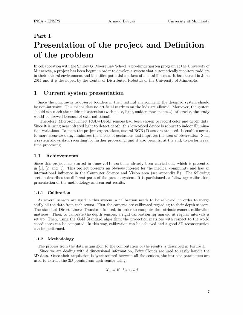
The process from the data acquisition to the computation of the results is described in Figure 1.Since we are dealing with 3 dimensional information, Point Clouds are used to easily handle the
3D data. Once their acquisition is synchronized between all the sensors, the intrinsic parameters areused to extract the 3D points from each sensor using:
Xw = K−1 ∗ xc ∗ d
7

INSA - ENSPS Arnaud Bruyas University of Minnesota
Figure 1: Methodology (extracted from [3])
where Xw is a 3D world point, K is the matrix of intrinsic parameters, xc the image coordinate andd the depth value from the sensor. Using the extrinsic matrices parameters, we can then carry all thedata from each sensor in a consistent common frame of reference.
In order to reduce the number of computable points and to delete the useless points from the pointcloud, a background subtraction is performed. After down-sampling the original point cloud by two,a background model is learned over a multitude of sample frames using the Robust PCA approach.After being vectorized, all the frames are concatenated in a matrix which is used to extract the stablebackground. At the end, a mask is created to filter out the background of the general Point Cloud.
After filtering the foreground points in order to reduce the noise, the next step consists in segmentingthose point clouds. Several algorithms have been tested. The first is based on the Euclidian distancebetween each point, to create clusters which represent each object of the foreground. Using thisdistance, a point’s neighbour may join its clusters if they are close enough. Once clusters are created,labels and bounding boxes are added to the depth image, and are used to attribute an RGB pixelinformation to each 3D point. Other segmentation methods have been explored and tested, such as agraph-based segmentation algorithm developed by Felzenszwalb et al. in [4]. In this case, each point isconsidered as a node which is a feature vector representing each point. It contains X,Y,Z location andRGB values of the point. The objects are considered as a group of supervoxels, which are computedusing the Euclidian distance between nodes.
In order to be easily tracked over time and space, Covariance Descriptors are computed for eachobjects (clusters) detected in the foreground. It is an efficient, robust and compact way to represent animage region, using features derived from the color and depth information (position, derivate of imageintensity for instance). Their size do not depend of the computed region, consequently, fast comparisonsare possible. More details about the covariance descriptors will be provided in the following sections(see 3.4.3 page 14).
In order to monitor toddlers’ behavior, the key issue is the tracking task. It is performed by twoalgorithms. The main tracking task uses a Kalman filter. Extracted objects are modelled by theircentroid position (x, y) and by an ellipsoid (6 parameters) to represent their shape. These parameters,as well as the velocity of the centroid are used as the state vector in the Kalman filter. Usual Kalmanequations are set up to perform the algorithm and insure the tracking task. However, this is not alwayssufficient and a covariance descriptor based algorithm may be set up to connect tracks of the sameindividual that happen to be broken. To compare two descriptors, The Log-Euclidean distance metricbetween them is used, by projecting those covariances onto a Euclidean tangent space [5].
Once all the parameters and all the algorithms have been set up, the next step consists in thebehavior analysis.
8

INSA - ENSPS Arnaud Bruyas University of Minnesota
1.1.3 Behavior analysis and results
Several experiments can be run with this system, from spatial occupancy to social interactions. Asurvey of previous run tests is developed in the following section.
Using tracking information, children spatial occupancy can be computed, in order to underline aneventual repetitive behavior, which is a common symptom of OCD [2]. An occupancy grid has beenset up and implemented using centroid positions. Indeed, frequent returns to a specific location in theroom, or a lack of movement in another one may highlight a behavior disorder.
The use of covariance descriptors combined with Kalman tracking also allows the access to thecentroid velocity. Those parameters can be used to quantify the children’s activity [3]. A high or aninsufficient level of motion could show physical handicaps or mental deficiencies.
In addition to these individual information, this system can also provide data about group behaviorand social interaction. In [1], a function has been set up to quantify the connectivity between twopeople, using their relative position and orientation at a given time. This instantaneous score is storedin an affinity matrix representing the interaction rate between observed people. Using this matrix,an embedding graph can be created, showing with segments and nodes the different interactions andtheir intensities. Moreover, using the ellipse shape attributed to each person, a differentiation couldbe made between adult and children, which allows analyzing toddler \ caregivers interactions. It couldbe useful to evaluate the impact of the caregiver related to interactions between a child and his peers.
Since the project and the current achievements are presented, the following sections will presentmy future work in this project, describe it and introduce his main parts.
2 Definition and description of my work in the project
This section is organized as follow. The first part introduces, explains and details the subjects of mywork. Then, a brief overview of similar researches is presented in the second part.
2.1 Definition of the subject
According to the studies described in [6] and [7], experiments can be run to focus on other at-risk markers or other behavior characterizations like arm and hand flapping or unsymmetrical armmovements. The current system doesn’t enable such studies because of the sensor specificities. Indeed,the cameras don’t have a high enough definition and don’t afford the opportunity of zooming oninteresting body parts, such as heads, hands, or even the full body.
That’s why, during my internship, I will focus my work on the following subject:
Integration of Pan-Tilt-Zoom camera in a multi RGB+D sensor system in order to gethigh resolution data for behavior analysis of children.
Several key issues can be highlighted in this project. One of my main focuses will be the control ofthe PTZ camera, regarding to the project needs and to the existing laws and algorithms. The servoingshould also take into consideration data acquisition requirements, which involve the setup of a robustperson tracker.
Moreover, as it will be a part of an existing system, the term ”Integration” is highly important. Itsuggests an accurate and synchronized calibration to get similar data. It also implies a communicationprocess between the existing system and the PTZ sensor. It results in the development of a master/slavetype relation, where the multiple RGB+D sensors system acts as the master and the PTZ camera asthe slave.
9
INSA - ENSPS Arnaud Bruyas University of Minnesota
Another key point is the gathering useful data regarding to the behavior analysis. A HD PTZcamera should allow to focus and track different members of the body and to collect data about it.This involves an accurate camera servoing and the setup of image processing to follow a kid in realtime.
2.2 Related and similar projects
This part lists and presents a few projects that are interesting due to their similarities with the one Iam working on.
In [8], a multiple sensor system is used to get biometric imagery of humans. It consists in a PTZslave camera monitored by a wide field of view master camera. While the master camera is used todetect humans, the PTZ camera tracks them and takes high resolution biometric imagery. Using twodevices allows monitoring a wide field of view and in the meantime, getting accurate biometric dataof a subject. This system is divided in three processes. The master process which takes continuouslyRGB information from the master camera, detects a person, computes several parameters about him,like his position, his velocity..., and transmits them to the Slave camera process. While it is listening tomaster camera process, this second process computes the slave camera information to track the personand control the Pan Tilt system. Then the third process consists in the control of the Pan-Tilt Unit(PTU) according to the parameters given by the Slave camera process. Although the Master processcould control the PTU process, this one could also be independent, using the Slave camera process. Itis an interesting hybrid Master/Slave relation that could be setup in our system.
With regards to the Master-Slave correlation, this system uses a special calibration. The purposeis to determine the relationship between the same spatial points projected in the image frame of bothcameras. The approach is as follows. For a set of actual points in the scene, their pixel positions inthe master camera image and their pan tilt angles used to center them in the slave camera image areboth recorded. Then, for any pixel points of the master image, an approximate pan tilt angle couldbe found using an interpolation between two sampled points. In this case, the knowledge of the realMaster/Slave relative position isn’t needed. However, the accuracy of the Pan Tilt control is reduced.But since a visual based detection and tracking is also performed by the slave camera process, thiskind of calibration is appropriate for this particular project.
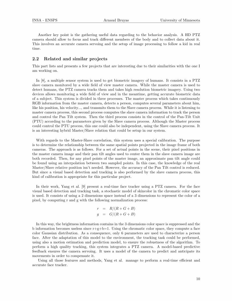
In their work, Yang et al. [9] present a real-time face tracker using a PTZ camera. For the facevisual based detection and tracking task, a stochastic model of skincolor in the chromatic color spaceis used. It consists of using a 2 dimensions space instead of a 3 dimensions to represent the color of apixel, by computing r and g with the following normalization process:
r = R/(R+G+B)
g = G/(R+G+B)
In this way, the brightness information contains in the 3 dimensions color space is suppressed and theb information becomes useless since r+g+b=1. Using the chromatic color space, they compute a facecolor Gaussian distribution. As a consequence, only 6 parameters are used to characterize a personface. After the adaptation of this model to the environment, the tracking task could be performed,using also a motion estimation and prediction model, to ensure the robustness of the algorithm. Toperform a high quality tracking, this system integrates a PTZ camera. A model-based predictivefeedback ensures the camera servoing. It uses a model of the camera to predict and anticipate itsmovements in order to compensate it.
Using all those features and methods, Yang et al. manage to perform a real-time efficient andaccurate face tracker.
10

INSA - ENSPS Arnaud Bruyas University of Minnesota
Part II
Related Work
3 Project key points and related works
This part focuses on the main issues highlighted in section 2.1 (see page 9) by explaining them andpresenting related researches and existing solutions.
3.1 Master/Slave relation
As the system will be composed of two different parts, a Master/Slave procedure is mandatory. Twokinds of relation can be set up: strict and hybrid.
The first one is a simple link where the PTZ camera doesn’t have any self-control. Position ordersare given by the master system and the slave only executes it. In this case, a 3D point data is providedby the RGB+D system and the PTZ camera sets its parameters (pan, tilt and zoom) according to it.Consequently, each time a movement of the PTZ camera is required, the master system needs to givean order.
In [8], a hybrid master/slave relation is developed. It is used to track a person and acquire biometricdata. It consists in a three-tier architecture. This system has already been described in a previoussection. It has the advantage of performing separatly the detecting, the tracking and the PTZ controltasks. Thus, the computation time is reduced, which could be useful for real-time applications.
3.2 Calibration
To insure a good integration of the PTZ camera and an accurate data acquisition, a good calibrationof the camera is required. Two different calibrations need to be achieved: the intrinsic parameters,which concern the camera itself, and the extrinsic parameters, which calibrate the geometric positionof the PTZ unit regarding to the other sensors.
3.2.1 Camera model
In [10], Sudipta et al. use a common model of camera called the pin-hole camera model. As assumedin [10], considering our use of the PTZ camera, we could also assume that the center of rotation of thecamera is fixed and coincides with the camera’s center of projection.
In this model, for the perspective camera, a point X in the 3D space is projected to x in the 2Dspace. It can be represented by : x = P.X, with P being the 3 ∗ 4 rank-3 camera projection matrix.The matrix P can be decomposed as follow:
P = K.[R−Rt] (1)
where K represents the intrinsic matrix, R the rotation and t the position of the camera regarding tothe world reference.
In this way, intrinsic and extrinsic parameters can be computed separately.
3.2.2 Intrinsic parameters
These parameters are independent of the camera position and orientation. In [10], the intrinsic pa-rameters are defined in a matrix as follow:
K =
αf s px0 f py0 0 1
11

INSA - ENSPS Arnaud Bruyas University of Minnesota
where px and py are the pixel coordinates of the principal point, f the focal length and α the camera’sx:y pixel aspect ratio. We assume that s, the camera’s x:y skew is equal to zero.
An important thing to consider is the variability of those parameters regarding to the value of thezoom. In [10], those intrinsic parameters are computed for discrete zoom levels, and the completeintrinsics are obtained by linear interpolation.
3.2.3 Extrinsic parameters
These parameters are used to find the geometric position of the camera in the world reference. Asdiscussed in [11], two kinds of geometric relation can be used. The first one use a look-up tablewhich links 3D world point with pan-tilt angles; whereas the second one computes the real geometricalposition of the camera with respect to the world reference.
The first method is also used in [8]. It needs a learning step, where the p, t z parameters and 3Dworld points are manually correlated in a look-up table by using different points of interest. Then forevery 3D world points, p,t and z parameters can be estimated by a linear interpolation.
The second method consists in computing the real geometrical position of the PTZ camera in theworld reference, which becomes the common frame between all the sensors. Several algorithms can beimplemented to estimate that position. First, the current method applied for the RGB+D sensors usesa rigid calibration rig. Since the size and the orientation of this rig are known, image of it with thePTZ camera can be used to approximate it position. A method is developed, in [12], using the DirectLinear Transform (DLT) algorithm. It consists in estimating the Camera Matrix P (see equation 1)knowing the 3D world and the image coordinates of a set of points. Moreover, another form of P canbe as follow:
P = K.[R| −R ∗ C] (2)
with K, the intrinsic matrix, R the rotational matrix between the two references and C the centre ofthe camera.
Moreover, since the Depth sensor system allows easy access to the 3D point position, they can beused to detect the PTZ camera and from there, estimate its position. This method implies that thePTZ unit is in the field of view of the Kinect sensors system.
Those methods would be implemented to estimate the position of the PTZ camera, but the ori-entation given by the camera optics’ axis, is related to the Pan and Tilt angles. Simple geometricfeatures ensure the correspondence between the 3D point coordinate (X’,Y’,Z’) and the p and t pa-rameters, such that the principal axis of the camera is oriented toward this point. It uses correlationequations between Cartesian and Spherical frames. The computed angles could also be used to controlthe camera.
The choice of one of these calibration methods is highly related to the chosen PTZ camera controllaw.
3.3 PTZ camera servoing
Two different parts should be considered: the pan-tilt angle to follow the target and the zoom to keepa correct field view.
3.3.1 Pan-tilt control
Currently, a lot of tracking system uses a visual servoing approach [13] and a lot of studies describeit [14], as well as tutorials [15] [16]. Judging by the results obtained in related works and by theapplication we want to design, a visual servoing approach can be a good solution to control our PTZsystem. The visual based approach consists in the minimization of an error e(t):
12

INSA - ENSPS Arnaud Bruyas University of Minnesota
e(t) = s(m(t), a)− s∗
where m(t) is a set of image measurements, a is a set of parameters that represent potential knowledgeabout the system, and s* the desired values of the features. In our case, m(t) is the pixel position xand y of the target at the instant t and s* is the center of the image frame. Considering our systemas a eye-in-hand robot, we could use this equation (described in [16]):
s = Js.q +δs
δt
and
Js = Ls.VN .J(q)
with Js being the feature Jacobian matrix; composed by VN , the transform matrix from the camerareference to the robot reference, J(q) the robot Jacobian and Ls the interaction matrix. Judging by thecamera geometry, J(q) could be calculate, and using the method describes in [15], we could computeLs.
Since an exponential decrease of e is to be ensured (e = λ.e), the following control law is obtain:
q = −λJ+e e− J+
eδe
δt
where Je = Js and J+e = (JT
e .Je)−1.JT
e , the pseudo-inverse of Je.It is important to notice that this law considers the time variation of e due to the generally unknown
target motion.Applied to a PTZ unit, this servoing method should give satisfying results regarding to time
computation and accuracy. Nevertheless, it needs an image processing algorithm to find the trackedtarget in the image frame and generate e.
3.3.2 Zoom control
In our system, the zoom feature is used to get close view of children. Therefore, a zoom servoing isneeded to ensure the same close focus on the child while he is moving in the room. This servoingcould be independent of Pan Tilt angles and only depends of the images of the camera. Or it could beadjusted judging by the Pan-Tilt parameters. Indeed, the p and t parameters carry information aboutthe camera orientation, and knowing it position, the z parameter could be adjusted.
3.4 Target detection
In our application, the target is a toddler or a part of his body, such as his hand or his head. Therefore,the selected method should be adjustable to different patterns, using a learning period or not. Eachdetection algorithm has a theoretical fundament, which could be prohibitive for a particular application.For instance, since the image field is moving, a background subtraction can’t be easily computed. Inthe following part, different types of algorithms are detailed, with a focus on covariance descriptors,because it is the method implemented in the current system.
3.4.1 Skin color detection
These types of algorithms are based on the skin color detection in the image. They are used for peopleidentification, or to track people’s faces. In [9], the authors show that a common skin-color patternexists in a normalized color space (as developed in 2.2 at page 10), that could be used to detect everypeople face. In [17], Stilmann et al. describe the shape of those histograms by a two dimensionalGaussian repartition. In this way, a face person is characterized by only five parameters, which allowsto perform a fast people identification.
13

INSA - ENSPS Arnaud Bruyas University of Minnesota
3.4.2 Movement detection
If the target is in motion, several algorithms can be applied using this time and space feature thatis the movement. For instance, Zhou et al [8] uses a combination of Frame Differencing and MotionHistory with sparse optic flow.
But for our system, motion detection may not be a good feature, because a child could stay at thesame place for a while, which is a problem for motion detection.
3.4.3 Covariance descriptors
As describe in section II, covariance descriptors are already used in this project to detect and tracktoddlers with RGB+D data. This type of region descriptors is computed on a region of interest.
In [18], Tuzel et al. describe a fast way to compute covariance descriptors, which can be used toperform real-time tracking, as it is shown in the study. Their paper presents several main contributions:the use of covariances as a feature, a fast way to compute covariances using integral images and newalgorithms for covariance features applications.
Covariance descriptors are a fast and powerful way to represent a point cloud. For each point cloudof an object, using image related data, a covariance descriptor is computed as follow:
CR =1
n− 1.
n∑k=1
(zk − µ)(zk − µ)T
where R is the region computed, n the number of pixels in R, zk the d-dimensional feature points, dthe number of features in the descriptor and µ the mean of the points for each features.
Using covariance descriptors as features to represent a point cloud is interesting because a singledescriptors of a region is enough to detect the same region in different views and poses. Moreover,covariance descriptors are low-dimensional and their size is independent of the computed region size.However, since covariance matrices do not lie on Euclidean space, the log-Euclidian distance metric(developed in [5])is used to compare them and perform identification or tracking tasks:
dist(C1, C2) = ‖logC1 − logC2‖ (3)
In [18], Tuzel et al. also present a fast way of covariance computation, using the d-dimensionalfeature image extracted F (x, y). Then covariance descriptors CR of the region R[(x′, y′), (x′′, y′′)]canalso be computed with the first order integral tensor P and the second order integral tensor Q of theimage, as shown below:
CR(x′,y′,x′′,y′′) =1
n− 1.[Qx′′,y′′ +Qx′,y′ −Qx′′,y′ −Qx′,y′′
− 1
n(Px′′,y′′ + Px′,y′ − Px′′,y′ − Px′,y′′)(Px′′,y′′ + Px′,y′ − Px′′,y′ − Px′,y′′)T ]
with P and Q defined as follow:
Px,y = [P (x, y, 1) . . . P (x, y, d)] with P (x′, y′, i) =∑
x<x′,y<y′
F (x, y, i)
Qx,y =
Q(x, y, 1, 1) · · · Q(x, y, 1, d)...
...Q(x, y, d, 1) · · · Q(x, y, d, d)
with Q(x′, y′, i, j) = sumx<x′,y<y′F (x, y, i).F (x, y, i)
14

INSA - ENSPS Arnaud Bruyas University of Minnesota
Depending on the information given by the sensors, covariance descriptors can be made up of differentfeatures. For a detection task, Tuzel et al use nine features: X and Y positions, RGB values and firstand second derivatives of color intensities. But in [3], 12 features are mentioned, including gradientorientation and gradient magnitude. In [2], 10 more features are added concerning distance data andtheir derivatives, which create a 22*22 covariance matrix.
3.5 Optimization of the descriptors composition
Obviously, the number of features is highly related to the computation time, but also to the efficiencyof those descriptors; because depending of the descriptor target, some features are more relevantthan other. So in order to perform an accurate and real-time covariance descriptor computation, thenumber and the type of features should be optimized. A lot of different combinations of features couldbe performed among all the possible one. The problem is to modify the composition of the covariancedescriptors in order to minimize the time of computation and maximize the efficiency of the trackingtask. This is a Multiple Objectives Combinatorial Optimization (MOCO) problem. In [19], severalalgorithms are introduced to solve optimization problems, but only a few could be applied in this case.Two of them are introduced in the following parts: a Simulated Annealing method and a GeneticAlgorithm.
3.5.1 A Simulated Annealing method
Judging by the difficulty of this problem and the areas of application developed for each algorithmin [19], the Simulated Annealing method may be a good optimization technique. After presenting ausual Simulated Annealing algorithm, Czynak et al. [20] propose an amelioration of this algorithmusing a sample of so-called generating solutions, in order to optimize several objectives.
In our case, we want an efficient and quickly computed covariance descriptor. So the parametersto optimize are the time of computation and the tracking accuracy. An overview of the algorithmextracted from [20] and adapted to our case is presented in Algorithm 1
In Algorithm 1 α is close to 1 and P (x, y,Λ, T ) is a multiple-objective rule for acceptance probability.Several laws could be used, such as:
P (x, y,Λ, T ) = min
{1, exp
(max
j(λj .(fj(x)− fj(y))/T )
)}
P (x, y,Λ, T ) = min
1,
2∑j=1
(max
j(λj .(fj(x)− fj(y))/T )
)In this algorithm, V (x) represents the neighbourhood of x. It is the set of possible solutions that
could be reached from x by making a simple variation. In our case, this variation would be thesubstitution or the addition of a feature in the covariance descriptor.
3.5.2 A Genetic Algorithm
Using a Genetic Algorithm can be another way to solve this MOCO problem. Genetic Algorithms(GA) were first implemented based on the model of biological Evolution. Usually, they consist of fourgeneral steps: Initialization, Selection, Reproduction and Termination and are performed on fictivechromosomes representing possible solutions. As many GA variations have been adapted to variousproblems, for our Multiple Objectives problem (MOp) different approaches are available (see [21] for apartial survey). The first possibility is to combine all the objectives into a single weighted sum. Thishowever can lead to compromised solutions. Since several objectives are involved, it becomes difficult
15

INSA - ENSPS Arnaud Bruyas University of Minnesota
Algorithm 1: Simulated Annealing Algorithm
Data: D: the set of all possible solution, regarding to features’ number and naturefj : Objectives to optimize, f1 time of computation and f2the efficiency of the tracker using thecomputed descriptorM : a set of potentially efficient solutionsT0: Initial temperature of the systemT : current temperature of the systemΛ = [λ1, λ2], the weighting vector
Select several solutions x ⊂ D and P0 ← x;
for i← 0 to sizeofP0 doM ← x;
T = T0;repeat
construct y ∈ V (x) a neighbour of x;if y better than x then
remove x and add y to M ;else
Select the solution x′ ∈ S closest to x but still better than x;if x′ don’t exist then
set random Λ such that λ1 + λ2 = 1;else
for each objectives fj do
λj =
{αλj if fj(x) ≥ fj(x′)λj/α if fj(x) ≤ fj(x′)
such that λ1 + λ2 = 1;
switch y and x in S according to P (x, y,Λ, T );
if the conditions of changing T are fulfilled thendecrease T ;
until the stop conditions are fulfilled ;
16
INSA - ENSPS Arnaud Bruyas University of Minnesota
to identify a single best solution, and depending of the importance accorded to each objective, severalmight be chosen.
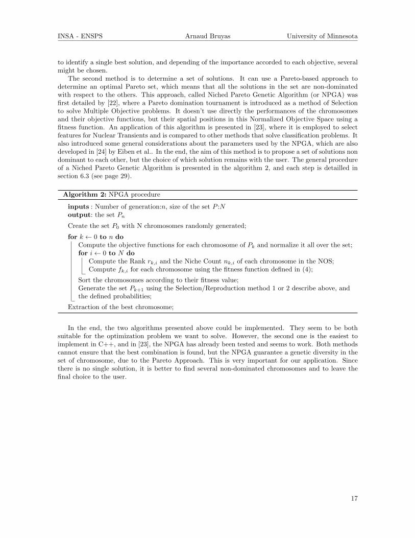
The second method is to determine a set of solutions. It can use a Pareto-based approach todetermine an optimal Pareto set, which means that all the solutions in the set are non-dominatedwith respect to the others. This approach, called Niched Pareto Genetic Algorithm (or NPGA) wasfirst detailed by [22], where a Pareto domination tournament is introduced as a method of Selectionto solve Multiple Objective problems. It doesn’t use directly the performances of the chromosomesand their objective functions, but their spatial positions in this Normalized Objective Space using afitness function. An application of this algorithm is presented in [23], where it is employed to selectfeatures for Nuclear Transients and is compared to other methods that solve classification problems. Italso introduced some general considerations about the parameters used by the NPGA, which are alsodeveloped in [24] by Eiben et al.. In the end, the aim of this method is to propose a set of solutions nondominant to each other, but the choice of which solution remains with the user. The general procedureof a Niched Pareto Genetic Algorithm is presented in the algorithm 2, and each step is detailled insection 6.3 (see page 29).
Algorithm 2: NPGA procedure
inputs : Number of generation:n, size of the set P :Noutput: the set Pn
Create the set P0 with N chromosomes randomly generated;
for k ← 0 to n doCompute the objective functions for each chromosome of Pk and normalize it all over the set;for i← 0 to N do
Compute the Rank rk,i and the Niche Count nk,i of each chromosome in the NOS;Compute fk,i for each chromosome using the fitness function defined in (4);
Sort the chromosomes according to their fitness value;Generate the set Pk+1 using the Selection/Reproduction method 1 or 2 describe above, andthe defined probabilities;
Extraction of the best chromosome;
In the end, the two algorithms presented above could be implemented. They seem to be bothsuitable for the optimization problem we want to solve. However, the second one is the easiest toimplement in C++, and in [23], the NPGA has already been tested and seems to work. Both methodscannot ensure that the best combination is found, but the NPGA guarantee a genetic diversity in theset of chromosome, due to the Pareto Approach. This is very important for our application. Sincethere is no single solution, it is better to find several non-dominated chromosomes and to leave thefinal choice to the user.
17

INSA - ENSPS Arnaud Bruyas University of Minnesota
Part III
Planning of the projectIn this section, the work I plan to achieve is presented, as well as an estimation of the time schedule.
3.6 Considered work
First, I will develop a program to connect the PTZ camera to the computer, which allows controllingit and getting images from it. Depending on the camera and its environment, the amount of workneedes for this task will be variable. Then I plan to achieve a detection algorithm in several imagescaptured by the camera, using covariance descriptors. In this way, the targeted pattern position canbe computed in the camera image. That position information should be used to perform an imagebased servoing using the PTZ camera, to follow a child for instance. In order to carry out real-timeservoing, an optimization algorithm will be computed to find the best features used by the covariancedescriptors.
3.7 Time schedule
Figure 2 shows an overview of the time schedule planned for this project.
Figure 2: Time schedule for the project
18

INSA - ENSPS Arnaud Bruyas University of Minnesota
Part IV
Achieved Work, Results and CommentsThis part describes the work carried out during my internship. First, the way of controlling thecamera will be presented. Then, working with this, a tracking algorithm has been implemented, usingcovariance descriptors. Finally, in order to perform a real-time tracking as efficient as possible, thefeatures used by the descriptors had been optimized using a Genetic Algorithm.
4 Camera Setup and Control
As detailed in [1], [2] and [3], the current system is using RGB+D sensors to collect video data. Thosedevices present several advantages. They are cheap, easy to setup in the classroom, non invasive andportable (they can be removed after the tests). The two last conditions are essentials because theyare mandatory and are mentioned in the grant specifications. The goal of the developed system is todetect at-risk markers that can highlights mental illnesses. Some of them are developed in [6] and [7].The current system allows the detection of several of them, but for others, another device is required,with a better definition and/or a zoom features.
So the idea is to add to the current sensors one or two PTZ cameras with High Definition images.Such a device allows close captions of objects or persons using the zoom, and by controlling the Panand Tilt angles, a tracking task can be performed.
4.1 Camera Specifications
Before buying a new PTZ device, my work was to use an old one to show that a real-time tracking isfeasible. Therefore, a Panasonic with an AXIS video converter had been used, both available in thelab. The AXIS device gives access to an API [25] to configure and control the camera. So by usingURL request as detailed in [25], the camera can be controlled and images and videos can be retrieved.To send the URL requests to the video server, a C++ library has been implemented in the project. Itis called libcurl and presented in [26]. It permits to easily submit URL request to the camera throughthe network, in order to move it. Then video streaming is handled using OpenCV [27]. The use ofthose two libraries enables a full control of the camera, from video recording to Pan, Tilt and Zoommovements.
However, only relative movements are possible with the driver provided on the AXIS website forthis particular camera. The zoom is moved by defining a number of mechanical steps, and the Pan andTilt actions are defined by the angle value of the movement in degrees. This is not a problem becausedepending on the feedback carried out thereafter, an absolute control can still be easily implementedin the software.
Then the first tests were run to see the performances of the camera : accuracy and repeatability.The following experiments have been designed in order to qualify the zoom of the camera. A patternsquare has been measured in different images grabbed at a zoom value incremented by 100 steps eachtime. The measured distance is in pixels. The goal of this experiment was first to observe the shape ofthe zoom magnification. Given a length in the image, what would be the zoom movement to enlargeit by a certain coefficient? Moreover, by running the same experiment several times, the repeatabilitycan be observed too.
As we can observe in Figure 3, the shape of the magnification is exponential. But the repeatabilityof the process seems to be variable, because the more important is the zoom value, the more differentthe length of the pattern is. Therefore, other experiments have been carried out, in order to evaluatethe repeatability of the zoom feature. In the first one, a zoom in and then a zoom out commands ofthe same amount are accomplished, and the size of a same pattern in the image is measured each time
19

INSA - ENSPS Arnaud Bruyas University of Minnesota
Figure 3: Size of the same square in the image for different zoom steps
Figure 4 displays those measures. As observed on the graphic, there is an important variation amongthe values. That implies a very bad repeatability, and makes impossible the creation of an absolutecontrol of the zoom. The same experiment has been run on the Pan and Tilt features and the sameconclusions can be made. Therefore, another way to control it needed to be setup, since the acquisitionof a new camera was planned, but only for the end of the summer.
4.2 Camera Control
First, another experiment has been designed, to figure out possible explanations to this inaccuracy. Aplausible reason is the delay between the moment the command to stop is sent and the moment thezoom device actually stop. So the following experiment has been designed. A zoom in (for instance+6x), and then a zoom out of the same amount divided in several steps (-2x, -2x and -2x) are performedseveral times in a row. Figure 5 shows the evolution of the size in pixels of a same pattern in thesedifferent frames.
As we can see, the distance decreases in the time. The same test has been run, but by zooming outfirst, and then zooming in several steps; and the reference length in the image increases. With theseresults, it seems that an offset appears each time that an URL request is sent to the camera. That’swhy a new control for the zoom has been tried, using only a unique request, repeated as many timeas needed. For example, to move the zoom to +3 units, the camera receives three times the command+1 unit. So the offset should compensate itself when the camera zooms out. But even this kind ofcommand didn’t work better than the previous since the offset is not constant.
Then a control by using the speed of the device instead of the position has been tried. By modifyingthe time between the command which sets a constant zoom speed and the one which sets it to zero,the zoom position can be controlled, and therefore the magnification. But this method presents aproblem. Another offset appears because there is a time difference between the moment the URLrequest is sent and the moment the camera really stops. Moreover, this time is not constant and it
20

INSA - ENSPS Arnaud Bruyas University of Minnesota
Figure 4: Size of the same square in different images after zoom in and a zoom out commands
Figure 5: Size of the same square in different images after zooming in 6x and a zooming out 3 times2x
21
INSA - ENSPS Arnaud Bruyas University of Minnesota
Figure 6: Simulation of the preset positions method
cannot be easily estimated. So unfortunately, this method is not better than the other one because wecan’t know exactly when the zoom’s movement starts and when it stops.
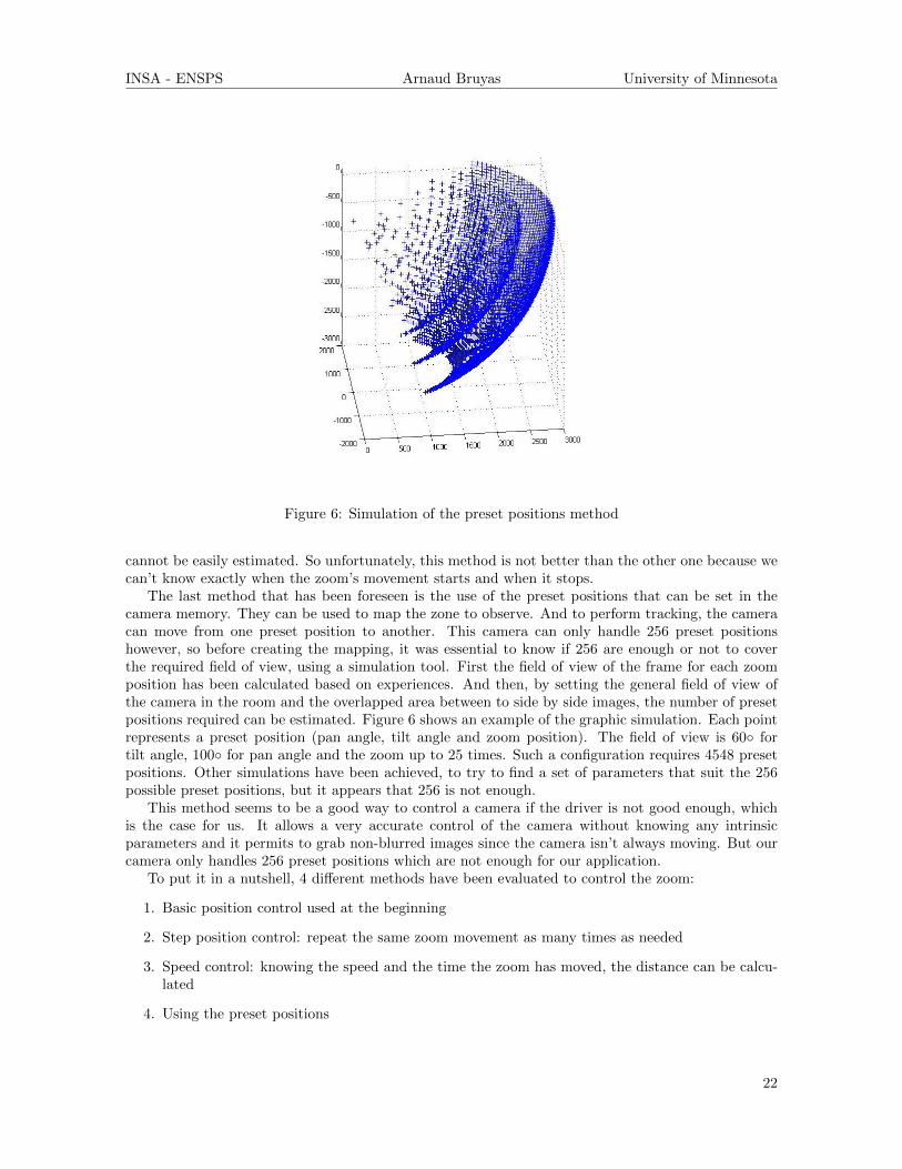
The last method that has been foreseen is the use of the preset positions that can be set in thecamera memory. They can be used to map the zone to observe. And to perform tracking, the cameracan move from one preset position to another. This camera can only handle 256 preset positionshowever, so before creating the mapping, it was essential to know if 256 are enough or not to coverthe required field of view, using a simulation tool. First the field of view of the frame for each zoomposition has been calculated based on experiences. And then, by setting the general field of view ofthe camera in the room and the overlapped area between to side by side images, the number of presetpositions required can be estimated. Figure 6 shows an example of the graphic simulation. Each pointrepresents a preset position (pan angle, tilt angle and zoom position). The field of view is 60◦ fortilt angle, 100◦ for pan angle and the zoom up to 25 times. Such a configuration requires 4548 presetpositions. Other simulations have been achieved, to try to find a set of parameters that suit the 256possible preset positions, but it appears that 256 is not enough.
This method seems to be a good way to control a camera if the driver is not good enough, whichis the case for us. It allows a very accurate control of the camera without knowing any intrinsicparameters and it permits to grab non-blurred images since the camera isn’t always moving. But ourcamera only handles 256 preset positions which are not enough for our application.
To put it in a nutshell, 4 different methods have been evaluated to control the zoom:
1. Basic position control used at the beginning
2. Step position control: repeat the same zoom movement as many times as needed
3. Speed control: knowing the speed and the time the zoom has moved, the distance can be calcu-lated
4. Using the preset positions
22

INSA - ENSPS Arnaud Bruyas University of Minnesota
Figure 7: Focal lenght on the X and Y axis depending on the zoom position
But any of these methods present the accuracy, the repeatability or the technical capacities neededfor an absolute zoom position. It appears that the problem is not the camera itself but the driver usedby the video encoder. So for an implementation in the lab-school, a new camera has to be purchased.
4.3 Movements Calculation
As shown before, the zoom device presents some weaknesses in the driver that make it unusable for anabsolute control. But, this absolute control is required for the calibration of the camera, since some ofthe intrinsic parameters depend on it, like the focal length. Indeed, a feedback is already performedby the camera itself in order to achieve the relative position control implemented. This can be used tocompute a relation between a position in the image and relative Pan and Tilt angles. This has beencarried out using a simple geometric relation.
This relation requires the knowledge of the intrinsic parameters, which have been computed usingOpenCV functions [27]. The values found are not accurate at all, since a good zoom control isimpossible. But the shape of the graphic of the focal length depending on the zoom value 7 seems tocorrespond to a typical one, and also match the values described in the datasheet of the camera.
Then some tests have been run to observe the results of the Pan and Tilt Command implemented.As expected, the accuracy is however very low due to the same problems mentioned before. Therefore,the implemented camera movement control can’t be evaluated with this camera.
23

INSA - ENSPS Arnaud Bruyas University of Minnesota
5 Tracking Task
The next step is the developement of a tracking algorithm. As mentionned before, it uses covariancedescriptor as a way to represent the target.
5.1 Computation of the Covariance Descriptor
As explain in [18], covariance descriptors are computed using image based feature. The image op-erations are made using OpenCV [27]. Those features can be of very different natures, for instancethe color channel, the pixel positions or any filter processing result. The color (R, G and B) featuresare directly extracted from the images, as well as the X and Y positions, and the first derivation arecalculated using Sobel filter. Then, all those information are put together to create the covariancematrix, using the formula described in 3.4.3 (see page 14).
Covariance descriptors present several advantages. They are compact, quickly computed and cancombined features of different natures. Therefore, they are a good way to represent any image.
The implementation in a C++ program is made so it can be easily computed. Each feature isapplied to the frame using a different function. The structure of this function is the same for all thefeatures. It has two arguments: the original frame and the feature related frame. The creation of thevector F as described in [18] is performed with a vector of pointers which are pointing on the featurefunction used. In this way, the choice of the features is made by adding or not the pointer to thevector.
5.2 Tracking Algorithm
A tracking task is the ability to recognize the same object in different time successive images. Forthe recognition task, the goal is to find the bounding box in the image for which the descriptor is theclosest to the model. Therefore, a way to measure the difference between two descriptors is required.In [18], it is explain that covariance descriptors are not lying on an Euclidian space, so the distancedetailled in 3 is used to compare two descriptor.
This is due to the special shape of the manifold. In [28], Cherian et al. develop a new distancebased on the Jensen-Bregman LogDet Divergence, and compare it to other distances. They prove thatthis distance is computed faster and that its performances are better. Consequently, it is the one usedin the algorithm.
add the distanceThe tracking algorithm is very simple. It looks for the best match in the image compare to the
model descriptor in each frame.
5.3 C++ Implementation
It has been carried out using imbricate FOR loops that generate at each iteration a new bounding boxin the frame, compute its descriptor and compare it to the model. Using a IF statement, the minimumdistance is recorded as well as the bounding box.
5.4 Toward a real time tracking
In order to make the tracking real-time, several improvements have been made on the implementationof the algorithm, using different techniques.
The first enhancement was on the computation of the descriptor. Indeed, 60% of the frame pro-cessing is dedicated to the calculation of the descriptor. So instead of calculating the features one afterthe other, a multi-threads task has been implemented to speed up the creation of the descriptor. Soat the end, instead of using 60% of the processing time, it was only 20% of it.
Then, the search for the best has also been enhanced, by defining a Region of Interest (RoI) inthe whole frame. Indeed, if the position in the last frame is known, and considering that the time
24

INSA - ENSPS Arnaud Bruyas University of Minnesota
between two frames is very small, we can compute an area in the image where the tracked object willbe. The definition of the RoI is based on the estimation of the position of the target in the next frame,knowing the previous positions. Two different models have been tested as position estimator. They arebased on the same principle: estimate a function that match the last positions and use it to determinethe next one. The first one uses a simple affine function and the second one uses a polynomial. Inboth methods, it is assume that the time between two frames is constant, and each position has beendecomposed on the X and Y axis.
For the first method, the hypothesis is that the speed of the target during 3 consecutive frames isconstant. So an affine relation between the two last positions can be calculated and used to estimatethe next one. This implies that 3 consecutive positions are on the same line, which can be true onlyif the time between two frames is very small.
On the other hand, the second method approximates that the acceleration is constant during acertain period, so the positions during this period respect a 2nd order polynomial equation. Hence,we have the following equations for the positions Pxi
according to the X axis:
Pxi= a0 + a1 ∗ xi + a2 ∗ x2i , i ∈ [1, 4]
Which can be turn into a matrix equation: ~Px = X ∗ ~a, with X a 4 by 3 matrix.Since the size of ~a is 3, 4 equations at least are needed to solve it, that’s why the 4 last points are
used. Then the solution is:~a = (XT ∗X)−1 ∗XT ∗ ~Px
Finally, knowing a0, a1, and a2, we can estimate the next position of the target.To test those two position estimation techniques, 150 consecutive target positions have been
recorded from a video and used to apply the two algorithms on Matlab. Figure 8 and 9 presentrespectively the two graphics obtained for the position projected on X axis.
Figure 8: Graphic presenting the real positions(red) and the estimated positions using a linear es-timation (blue)
Figure 9: Graphic presenting the real positions(red) and the estimated positions using a polyno-mial estimation (blue)
The average errors in pixels between the estimated positions and the real positions for the twomethods are as followed:
• Using a polynomial regression, the error is : 16.15 pix (X axis), 14.8 pix (Y axis)
• Using a linear estimation, the error is : 12.25 pix (X axis), 10.8 pix (Y axis)
25

INSA - ENSPS Arnaud Bruyas University of Minnesota
Results show that the linear estimation is better, which is confirmed by additional tests run withother tracking samples. Therefore, it is the method used to position the RoI. Its size has been adjustedby experimentation and has been found to be twice the size of the previous bounding box of the target.With respect to the size of the bounding box during the search, only three different sizes are testedin the algorithm: the same than the previous one, slightly larger and slightly smaller. Not all the sizehas to be tested, since the time between two frames is supposed to be very small. Regarding the scanof the RoI looking for the best match, not all the possible bounding boxes are tested. As mentionedbefore, only 3 different sizes are tested, and the positions are defined using steps in pixels. It createsa grid all over the RoI and reduces the number of comparisons.
Finally, it appears that moving the camera is also time consuming, since it implies to send an URLrequest and wait for the answer. So instead of performing a pin-point accurate tracking, the algorithmonly ensures that the target is in the field of view of the camera. Therefore, some theoretical limitshave been created in the image, and if the object goes past it, the camera is moving in order to centerthe image on the target. At the end, the algorithm implemented is presented in Algorithm 3.
Algorithm 3: Simple Tracking Algorithm
Initialisation of the position of the target and its covariance descriptor;
repeatGrab an image form the camera;Compute a Region of Interest where the target may be, using previous computed distanceand previous window size;Find the new target position in the RoI;if the target position is outside the fictitious limits then
Compute the Pan and Tilt angle;Move the camea;
until the stop condition is fulfilled ;
Using this algorithm, some tracking tasks have been tried to see the performance of the algorithm.It appears that the computing time for one frame is highly related to the nature and the number offeatures used in the object descriptor. Table 1 presents some examples in the tracking of a red cup.All of them present the same performance regarding to the accuracy of the tracking.
6 Optimization of the Descriptor’s composition
In this part is developed the implementation and the test of a Genetic Algorithm, designed to optimizethe combination of the features describing a given object. As explained before, this is a Combinatorialproblem. Knowing a set of possible features, the goal is to find the best one to describe an object inorder to perform the fastest and the most accurate tracking possible. For that purpose, the trackingalgorithm describes above is used as a black box with inputs and outputs.
6.1 Definition of the Problem and creation of the ground truth
As mentioned before, we chose to solve this combinatorial problem using a Genetic Algorithm. Thefollowing of this document assumes that the reader is familiar with the field of the GA, otherwise, aquick review is made in section 3.5 (see page 15). The objective function that compute the objectivevalues is the tracking algorithm describe before. For the necessity of the GA, it has been used as aBlack Box with inputs and outputs. In our case, the input is the combination of features used bythe covariance descriptor, and the outputs are the mean computational time of on frame (MCT), andthe Accuracy. The second output is the mean distance other all the frames, between the position of
26

INSA - ENSPS Arnaud Bruyas University of Minnesota
Features a MCT (s)
R,G,B,X,Y 0.049
R,G,B,X,Y,X’,Y’ 0.0754
R,G,B,X,Y,X’,Y’,X”,Y” 0.1096
R,G,B,X,Y,X’,Y’,X”,Y”,Mag 0.147
R,G,B,X,Y,X’,Y’,X”,Y”,Mag,Dir 0.1995
a X’ and Y’ are the first derivation of respectivelythe X and Y features, X” and Y” are the secondderivation of respectively the X and Y features,Mag is the magnitude of the gradient featureand Dir is the direction of the gradient feature.
Table 1: Comparaison table
the best match found in each frame and the ground truth position. Thus, the two objective values tooptimize are the MCT and the Accuracy. To perform the best tracking possible, both of them have tobe minimized.
To get the accuracy, the vector of reference positions for the tracked object in each frame has tobe known. It is created by pointing the object in each frame of the video sequence. But since thenumber of frame of each video is around 600, it would be very displeasing to point it out on everyframe, especially because the videos present a frame rate around 30 fps. So the position between twoframes is not very different. Thus, a method has been implemented using only the pointed positionsof the target every 10 frames. It assumes that between it, the object trajectory is linear and thatthe speed of the target is not too important. Then, the intermediate positions are computed using alinear regression. This technique divides by 10 the number of positions pointed, without affecting theaccuracy of the ground truth. Figure 10 presents the estimated positions in pixels and the approximateone, and Figure 11 shows the difference between them for each point. It doesn’t exceed six pixels,which can be ignored.
6.2 Creation of chromosomes as a good way to represent the descriptors
The first thing to define is a way to describe the problem using chromosomes. In our case, chromosomesare represented by a vector of Boolean, where each Boolean value is a gene, and each gene codes apossible feature. Hence, the size of a chromosome is fixed by the number of features that could be usedin the covariance descriptor. A ’0’ (false) in the gene sequence means that the corresponding featureis not used, and a ’1’ (true) means that it is. So a chromosome is then a fixed size vector containingBooleans that referring to features. This disposition implies an order between the features, whichprevent the creation of descriptors using the same features but in a different order. Moreover, it usesfixed length chromosomes, which are easier to handle than variable size one during the Reproductionstep. Figure 12 pictures an example of the process of chromosome creation.
Moreover, this representation enables an easy way for a random creation of chromosomes, which isthe first step of the GA. Using this representation, each chromosome is unique, and using the trackingalgorithm described before, its MCT and Accuracy can be determined as the objective values.
27

INSA - ENSPS Arnaud Bruyas University of Minnesota
Figure 10: Graphic presenting the real positions (red) and the estimated positions (blue)
Figure 11: Comparaison of the real and the estimated points over the time
28

INSA - ENSPS Arnaud Bruyas University of Minnesota
Figure 12: Diagram of the process for the creation of a chromosome
6.3 Description of the steps of the GA
As explained in the related work section, this is a Combinatorial Optimization with Multiple Objec-tive to minimize. The survey detailed in [21] highlights different methods to go through the multipleobjectives problem, and [23] presents a similar problem solved using a Niched Pareto Genetic Algo-rithm. Like all GA, it can be decomposed into 4 steps, describe in section ref3.5, starting with theinitialisation. A general view of the algorithm is settled in Algorithm 2.
6.3.1 Initialisation
The first step is the creation of the initial set of chromosomes. Its size is defined by the user and allchromosomes’ genotypes are generated randomly. Yet, some restrictions have been carried out. First,the minimum number of genes set to ’1’ in a chromosome is 3. Secondly, all the chromosomes of theinitial set are different to ensure the widest set possible.
6.3.2 Selection and Reproduction
This is the main process of the Algorithm, which lead the set toward the Pareto Front. First, theobjective values are computed for each chromosome, using the black boxdescribed before. Then, thesevalues are normalized all over the set, so they can be compared easily. After those two operations,each chromosome can be plotted in the Normalized Objective Space. This two dimensional space is agraphical interpretation of the set and acts as a basis for the computation of the fitness function. Theabscissa of it is the normalized MCT and the ordinate is the normalized Accuracy. Figure 14 displaysan example of a set in the NOS.
The next step is the computation of the fitness function for each chromosome, using the rank andthe niche count. As described in [21], there are several ways of assigning a rank to a chromosome, usingthe graphical representation of the set and the non-dominated criterion. In our case, a non-dominatedfront method is used. It attributes a rank of 1 to the chromosomes of the set that are non-dominated,virtually deletes them from the set and attributes a rank of 2 to the new dominant chromosomes.And so on until all the chromosomes are ranked. The fitness function also requires a niche countnumber. It is the number of chromosomes that are situated in the neighbourhood of a chromosome.This neighbourhood is defined by a circular region centred on the chromosome with a pre-determined
29

INSA - ENSPS Arnaud Bruyas University of Minnesota
radius. Then, using those two parameters, the Fitness function is calculated in the following way:
fi =2
ni + rki(4)
After being sorted from the best to the worse using the fitness value, the selection/reproductionis performed. Two different methods have been tested. The 1st one (called method 1) is classic.After computing the fitness values for each chromosome, they are sorted, starting with the best. ThenElitism is performed on the set, by keeping in the children set the best chromosomes of the fitnesssorted list. Then, reproduction is carried out on remaining chromosomes using crossover and mutation,according to preset probabilities.
The other approach (called Method 2) is based on High Elitism. It first selects all the chromosomeswith Rank 1 and adds them to the children set. Then, based on the fitness values computed for eachchromosome, Reproduction is performed. After being sorted, crossover is necessarily achieved on 2side by side chromosomes in the list. The number of permuted chromosomes during the crossover isproportional to the position of the chromosomes in the sorted list. In this way, only 1 gene is permutedon the best chromosomes, whereas half of the phenotype is modified for the worst one.
6.3.3 Termination Criterion
And the last step is the Termination. Different types of criterion can be defined to end the algorithm.The basic ones are the number of iterations or the computing time, but it can also be when there areno improvements in the solution quality. Using the last idea, a way to measure the set quality hasbeen set. Since we want to minimize the accuracy and the computational time, the closer to the axisin the Normalized Objective Space the chromosome will be, the better it is. That’s why the followingcriterion has been designed. It uses a point in the NOS, called the Quality Point. Projected all theway on the two dimensions of the graph, this point defined 2 zones with the axes: the Zone 1 withthe abscissa axis and the Zone 2 with the ordinate axis (see figure 13). Their sizes are defined by twoparameters, alpha1 and alpha2, which define the coordinates of the Quality Point. They both belongto [0, 1] since the objective space is normalized. By defining a minimum number of chromosomes ineach zone, a termination criterion can be created. Consequently, it requires 4 parameters:
• Alpha1: size of the zone1
• Alpha2: size of the zone 2
• %total: rate between the number of chromosomes in the zone1+zone2 and the total number ofchromosomes
• %zone1: amount of the previous number of chromosomes that are situated in zone1
Figure 13 presents a graphic display of this termination criterion. In the following, two differentend conditions will be tested: the one described above and a defined number of iterations.
6.4 C++ Implementation
All the steps described before have been implemented using C++ language, in order to be compatiblewith the tracking algorithm. A class have been created to represent the chromosome, with the followingattributes:
• A vector of Boolean, representing the genes
• Float : Accuracy
• Float : MCT
30

INSA - ENSPS Arnaud Bruyas University of Minnesota
Figure 13: Graphic of the different elements of the quality interpretation
• Float : Normalized Accuracy
• Float : Normalized MCT
• Int : Niche Count
• Int : Rank
• Float : Fitness Value
Several functions have also been created to compute random chromosome, set and get all theattributes, etc.
Regarding to the graphical display proposed, openCV [27] have been used. This graphical libraryallows to handle the image has matrices, and propose simple functions to draw line and circle and writetext on an image. Therefore, by knowing the size in pixel of the image, simple affine transformationsare required to adapt the NOS size to the image. OpenCV also integrate functions to deal with thevector.
Another tool has been developed as a complement of the graphical layout. A text file is generated foreach generation.It contains information about the chromosomes of the set: Genotype, MCT, Accuracy,Rank, Niche Count, and Fitness Value. It is used as a complement of the graphic, in order to ensurethe truthfulness of the results. Figure 14 presents an example of both tools. On the diagram, theabscissa is the Mean Time of Computation and the ordinate is the Accuracy, as defined above. In thisway, each chromosome can be plot in the NOS. The black dots are representing the chromosomes andthe green circle the Niche of the chromosome. The red number is used to identify the chromosome inthe report.
31

INSA - ENSPS Arnaud Bruyas University of Minnesota
Figure 14: Example of the display and the corresponding report
32

INSA - ENSPS Arnaud Bruyas University of Minnesota
Figure 15: Initial frame of the coffee box video, with a bounding box around the tracked object
6.5 First Tests
To test the algorithm and see its performances, the first tests have been run on a video not issued fromthe lab school video set. It was recorded with the PTZ camera presented before. A red cylinder (coffeebox) has been chosen as the target, because it presents a simple shape, a very recognizable colourand it is a non deformable object. Figure 15 presents the first frame of the video, with the boundingbox around the object. The use of this simple object is also a way to compare the different methodsimplemented for the Selection/Reproduction and for the termination criterion, since the results areeasier to interpret. Once the initial position of the object has been selected by the user, the NPGAcan be achieved.
Both Selection/Reproduction methods were tested, as well as both termination criteria.
6.5.1 Setup of the Experiment
The first tests have been carried out on an easy target (described in Figure 15), to observe the behaviourof the algorithm and examine its performances. The parameters have been adjusted experimentallyfor this video and are the following:
• Niche Radius = 0.1
• Crossover Probability = 0.5
• Mutation Probability = 0.05
• Number of chromosomes = 30
• Number of chromosomes selected by Elitism = 8
33

INSA - ENSPS Arnaud Bruyas University of Minnesota
Figure 16: Diagram of the final set of chromosome using the first method
6.5.2 Results
Since it is the first experiments, this part presents different Selection/Reproduction methods, as wellas different Termination Criterion, to find out which one seems the best for the NPGA.
The first test carried out was with the first method of selection and a defined number of generationsas the end condition. Figure 16 shows the final set in the NOS, and an evolution of the set is presentedin appendix A. Those 3 graphics emphasize the movement of the set toward the Pareto Front, andalso the expansion of the Front on his extremities. The shape of the front is consistent. Indeed, it isfollowing the two axes, and the goal is the minimization of both objectives, so the closer to the axis achromosome is, the better it is. Judging by the observations above, the first results of the NPGA arepromising.
The same test has been run using the second Selection method. The results are presented in Figure17 and in appendix B. The first observation is that some chromosomes are overlapping each other. Bycomparing their genotype, it happens that they are the same. This emphasizes the consistency of theobjective function (the tracking algorithm), since the same inputs give the same outputs.
It also appears that the concentration of chromosomes near the Pareto Front is more importantthan the first method. However, the repartition on this Front is way better for the final set of the firstmethod. Moreover, this technique seems faster than the first one, by comparing the graphical displayof the 20th Generation for both methods.
In order to compare in a better way these two methods, the termination criterion detailed in Figure13 has been implemented in the algorithm. Figure 18 presents an example of a final set using the secondSelection/Reproduction method and the following parameters:
• Alpha1 = 0.3
• Alpha2 = 0.4
• %total = 0.8
34

INSA - ENSPS Arnaud Bruyas University of Minnesota
Figure 17: Diagram of the final set of chromosome using the second method
• %zone1 = 0.5
More tests have been run, to observe the behaviour of new feature. They are presented in AppendixC. Despite the idea behind it, which was to monitor the shape of the Front, the results present someproblems. The first side-effect and the most unpleasant one is that if an outlier chromosome appears,because of the normalization process, the termination criterion will end the algorithm, even if it is thefirst generation.
Furthermore, the introduction of this new criterion implies the use of 4 more parameters to dealwith. So it seems that this termination criterion brings more trouble than solutions. Moreover, the useof Elitism in both selecting methods ensures that the best chromosomes are kept from a generation toanother. Therefore the convergeance toward a better set is mandatory. So the use of a large numberof generation as an end condition is suitable. The next test is using a set of 60 chromosomes over 80generations. For a more confortable display, the representations of the niches and the numerotationof the chromosomes have been deleted. Figure 19 and 20 respectively displays the initial and the finalset of chromosomses using the first method of selection.
Some observations can be made on the evolution of the set. The use of more chromosomes highlightsthe migration of the set toward the Pareto Front Zone , and propose at the end a better choice to theuser for the best chromosome. In comparaison, the second selecting method have been applied usingthe same parameters, and both initial and final sets are presented repectively in Figure 21 and 21.
The second method presents also good performances, since the concentration of chromosomes onthe Front is higher than in Figure 20. But the Front is not as wide and the Reproduction method usedcreate a lot of identical chromosomes in the set, which reduce the number of possibilities.
6.5.3 Comments and chromosome composition
Regarding to the chromosome composition, table 2 presents the results of the two methods presentedin Figure 16 and 17. It details the composition of some chromosomes which can be concidered as thebest by the user.
35

INSA - ENSPS Arnaud Bruyas University of Minnesota
Figure 18: Diagram of the final set of chromosome using the second method and the treminationcriterion
Figure 19: Initial set of chromosomes using the firstSelection method with 60 chromosomes
Figure 20: Final set of chromosomes using the firstSelection method with 60 chromosomes
36

INSA - ENSPS Arnaud Bruyas University of Minnesota
Figure 21: Initial set of chromosomes using the sec-ond Selection method with 60 chromosomes
Figure 22: Final set of chromosomes using the sec-ond Selection method with 60 chromosomes
Figure Chromosome Composition MCT (s) Accuracy
Fig.16
3 R B X 0.0345 31.37 pix
6 R G Y 0.0395 31.56 pix
15 R G Y Y’ 0.0546 16.34 pix
Fig.17
3 R B X Y 0.0565 11.99 pix
6 R G X 0.0498 20.97 pix
14 R G X Y 0.0572 12.13 pix
Table 2: Composition, Mct and Accuracy of several chromosomes which can be concidered as the best
37
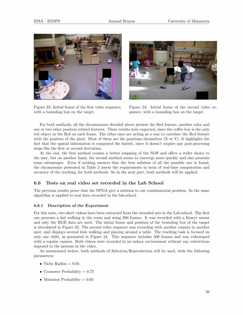
INSA - ENSPS Arnaud Bruyas University of Minnesota
Figure 23: Initial frame of the first video sequence,with a bounding box on the target
Figure 24: Initial frame of the second video se-quence, with a bounding box on the target
For both methods, all the chromosomes detailed above present the Red feature, another color andone or two other position related features. These results were expected, since the coffee box is the onlyred object in the RoI on each frame. The other ones are acting as a way to correlate the Red featurewith the position of the pixel. Most of them are the positions themselves (X or Y). It highlights thefact that the spatial information is computed the fastest, since it doesn’t require any post-procesingsteps like the first or second derivation.
At the end, the first method creates a better mapping of the NOS and offers a wider choice tothe user, but on another hand, the second method seems to converge more quickly and also presentssome advantages. Even if nothing ensures that the best solution of all the possible one is found,the chromosome presented in Table 2 meets the requirements in term of real-time computation andaccuracy of the tracking, for both methods. So in the next part, both methods will be applied.
6.6 Tests on real video set recorded in the Lab School
The previous results prove that the NPGA give a solution to our combinatorial problem. So the samealgorithm is applied to real data recorded in the lab-school.
6.6.1 Description of the Experiment
For this tests, two short videos have been extracted from the recorded sets in the Lab-school. The firstone presents a kid walking in the room and using 300 frames. It was recorded with a Kinect sensorand only the RGB data are used. The initial frame and position of the bounding box of the targetis introduced in Figure 23. The second video sequence was recording with another camera in anotherspot, and displays several kids walking and playing around a table. The tracking task is focused ononly one child, as presented in Figure 24. This sequence includes 500 frames and was videotapedwith a regular camera. Both videos were recorded in an indoor environment without any restrictionsimposed to the persons in the video.
As mentionned before, both methods of Selection/Reproduction will be used, with the followingparameters:
• Niche Radius = 0.05
• Crossover Probability = 0.75
• Mutation Probability = 0.05
38

INSA - ENSPS Arnaud Bruyas University of Minnesota
Figure 25: Representation of the final chromosome set in the NOS, using the Selection/Reproductionmethod 1 on a Real Data video
• Number of chromosomes = 60
• Number of chromosomes selected by Elitism = 24
6.6.2 Results and Comments for the first video sequence
Fig.25 and appendixDpresents the final configuration of the set using the first Selection/Reproductionmethod. From a qualitative observation, it seems that the shape of the Pareto Front appears moredistinctively. Moreover, the repartition of the set in the NOS is improved and the concentration aroundthe Pareto Front is augmented. Table 3 introduces the objective values of the chromosomes of the setselected as the best.
The second Selection/Reproduction method has also been applied on the same video sequence. Thefinal set configuration is exhibited in Fig.26 and Appendix E. It shows a Pareto Front with the sameshape than the previous one, even if the repartition of the chromosomes along it is unequal. However,the concentration of point in the interesting zone (close to the origin) is high, which can be interesting.The chromosomes chosen as the best are also described in Table 3.
Judging by the observations and charts specified below, several conclusions can be made regardingto the best descriptors composition. First, it seems that the use of color features is mandatory, andthat two of them at least are required. For this particular child in this particular environment, itseems that Red is the dominant color, since it is represented in nearly all the chromosomes of Table3. Moreover, regarding to the position features, the Y feature and its derivative is more representedamong the chromosomes than the X ones. It correlates the shape of a standing child, for which the Ydimension is more important than the X one.
By comparing the two Reproduction methods used, some distinctions can be made. As a result ofthe fitness-related selection performed, the repartition along the Pareto Front for the final set is betterwith the first method, which offer to the user a wider choice. The second method final set howeverpresents a better density of chromosomes around the area where the best chromosomes highlighted intable 3 are situated. In the end, it seems that both methods have some advantages, but as mentionned
39

INSA - ENSPS Arnaud Bruyas University of Minnesota
Figure 26: Representation of the final chromosome set in the NOS, using the Selection/Reproductionmethod 2 on a Real Data video
Figure Chromosomes Composition MCT (s) Accuracy
Fig.26
2, 11, 46 R B X Y Y’ 0.0864 33.64 pix
8, 57, 58 R B X Y 0.0652 43.72 pix
7, 43, 44 R G Y Y’ 0.0665 41.13 pix
5, 19, 50, 59 R G X 0.0555 45.71 pix
22 R B Y’ 0.0546 52.53 pix
Fig.25
26 G B X Y Y’ 0.0854 38.11 pix
11 12 42 R G Y Y” 0.0639 46.17 pix
8 R G Y’ 0.0571 48.07 pix
23 R X’ Y” 0.0580 76.52 pix
Table 3: Composition, MCT and Accuracy of several chromosomes which are concidered as the best
40

INSA - ENSPS Arnaud Bruyas University of Minnesota
Figure 27: Initial chromosome set for the secondvideo sequence, using the first selection method
Figure 28: Final chromosome set for the secondvideo sequence, using the first selection method
before, nothing ensure that the best combination possible is found, which is confirmed by table 3.Indeed, even if similarities can be highlight among the combinations displayed in table 3, there is nota single chromosome common to both method results.
6.6.3 Results and Comments for the second video sequence
The tracking child in this second vido sequence is described in figure 23. Since the results are moreconsistent using the first Selection method, it is the only one that had been implemented for this datasequence. The parameters used are the same than the previous video and the algorithm had been runover 48 generations. It leads to the final set presented in figure 28.
The final disposition of the set in the NOS is consistent, as well as the Pareto Front shape. Table3 highlights the composition of some of the chormosomes of the set.
As we can observe in the chart, the Blue feature is in every chromosome, which is consistentregarding to the tracked kid clothes. Moreover, the use of another colour features is strongly suggestedto reduce the number of features in the descriptor (see chromosome 0). But chromosomes 5 and 9 areshowing that the nature of this feature (R or G) is not very relevant.
Regarding to the position features, it seems that for this video, the axis (Y or X) is not veryimportant, which is relevant with the kid’s movements. He is not only walking, but also bending andrandomly playing. However, most of the chromosomes (8 out of 9) are using the first derivative of theposition (X’ and/or Y’) as a feature.
6.7 Conclusion on the GA performances
The results presented above are encouraging, since they highlight a selection of descriptors that seemsto match the tracked objects. The features selected in each case coincide with the object nature, suchas color for instance.Moreover, the chromosomes presented in the tables (2, 3 and 4) for each videosequence have similarities in their compositions, which is a proof of the convergence of the algorithm.
The creation of chromosomes as a very simple way to represent the descriptors helps a lot in thesetup of the Genetic Algorithm. Those fictive entities ensure an easy implementation of the different
41

INSA - ENSPS Arnaud Bruyas University of Minnesota
Figure Chromosomes Composition MCT (s) Accuracy
Fig.28
0 B X Y X’ Y’ 0.117 43.96 pix
1 R B X X’ Y’ X” 0.160 43.72 pix
2 R G Y Y’ 0.0665 36.9 pix
5 R B X’ Y’ 0.092 51.85 pix
9 G B X’ Y’ 0.093 53.28 pix
10 G B X’ Y” 0.109 61.48 pix
13 R B X’ 0.075 79.58 pix
14 R B Y 0.073 86.65 pix
15 R B X’ 0.074 82.5 pix
Table 4: Composition, MCT and Accuracy of several chromosomes in the final set presented in figure28
elements of the GA, like crossovers and mutations. They also make the principles of the algorithmmore understandable. Moreover, the use of a Normalized Objective Space as a way to get the fitnessfunction for each chromosome leads to a migration of the set toward the Pareto Front. According tothe selection method used, this front has different specifications in term of density and repartition. Thegraphical display also setup a tool for the final choice of one chromosome in the set by the user, sincethe NPGA presents at the end a whole set of chromosomes. The selection of a unique chromosome inthe set remains however to the user.
A possible continutation of this work can be the automatic selection of this chromosome. Indeed,methods like the boost method can use the combinations of the best chromosomes and create a newchromosomes using statistic tools and probabilities. Another improvement would be the use of newfeatures in the list, such as Gabor Filter, since one of the advantage of the covariance descriptortechnique combined with the NPGA is that any features can easily be added. This is emphazised bythe use of the OpenCV library which makes easier the computation of the features on any image.
42

INSA - ENSPS Arnaud Bruyas University of Minnesota
Part V
ConclusionDuring this internship, I had the chance to work on a cutting-edge project in Computer Science. As
part of the team my project was the integration in the system of a PTZ camera, in order to perform realtime tracking of a person. After developing a program that controls the camera, using URL requests,I focused my efforts on the design of an algorithm to perform a fast and accurate tracking. It employscovariance descriptors as a way to characterize the target. This fast and compact representationis computed using image based features. As developed in this document, the performances of thetracking are highly related to the features employed in the descriptor. Therefore, a Genetic Algorithmhas been carried out to solve this Multiple Output Combinatorial problem. It uses the trackingalgorithm achieved before as a way to compute the performances of a descriptor (the accuracy and thecomputational time). Then, by using chromosomes to represent a descriptor, a Niched Pareto GeneticAlgorithm is carried out, in order to optimize the composition of the covariance descriptors. The goalof this GA is to modify a set of chromosomes in order to improve it. In the end, this method givesto the user a set of chromosomes spread all along the Pareto Front, but the choice of a specific oneremains to the user.
Moreover, during this experience, I discovered the functioning of an American laboratory, which wasvery different from what I was expected. It is managed like a real company and the leaders expectsome results, like publications or journal papers. On the financial side, the amount of money involvedin the projects or received from national grants are around millions. As a consequence, there is someconstraint in the work to achieve. Furthermore, I also highly improve my technical English, since I hadto read and write all the documents in English. As a member of the Computer Science department,this internship was also the opportunity to improve my competences in this field. Therefore, I havebeen involved in other projects in which my program to control the PTZ camera has been used. I alsodiscovered many techniques and methods at the state of the art in the Computer Science, Vision orRobotics field.
However, the work is more personal than what I was thinking, since my supervisor was responsibleof 30 different people. Therefore, I had to figure out by myself how to define a subject. I also had tolearn by myself how to lead my research, even if the mutual help between all the students is important.In the end, the way of working is different. The students are more independant, and even if thesupervisors have an overview of every project, they let the students work by themselfes and trustthem.
Furthermore, the general chair of the ICRA 2012 was my supervisor. Thus I was present at theconference as a volunteer and I managed to attend to some talks and workshops. It was very rewardingto discover all the applications and all the possibilities in the Automation and in the Robotic fieldnowadays.
To put it in a nutshell, more than an internship, this experience was the opportunity for me to workin an American laboratory and discover its functioning. I also gain knowledge in the Computer Sciencefield and became familiar with the research process. It was for me a great experience and that’s whyI will pursue in the research area and begin a PhD in the IRCAD.
43

INSA - ENSPS Arnaud Bruyas University of Minnesota
Part VI
Appendices
44

INSA - ENSPS Arnaud Bruyas University of Minnesota
A Evolution of the chromosome set using the first selectionmethod on the coffee box video
45

INSA - ENSPS Arnaud Bruyas University of Minnesota
46

INSA - ENSPS Arnaud Bruyas University of Minnesota
47

INSA - ENSPS Arnaud Bruyas University of Minnesota
48

INSA - ENSPS Arnaud Bruyas University of Minnesota
B Evolution of the chromosome set using the second selectionmethod on the coffee box video
49

INSA - ENSPS Arnaud Bruyas University of Minnesota
50

INSA - ENSPS Arnaud Bruyas University of Minnesota
51

INSA - ENSPS Arnaud Bruyas University of Minnesota
52

INSA - ENSPS Arnaud Bruyas University of Minnesota
C Details of several tests run using the new termination cri-terion
53

INSA - ENSPS Arnaud Bruyas University of Minnesota
Figure 29: Final set of Test 1 Figure 30: Final set of Test 2
Figure 31: Final set of Test 3 Figure 32: Final set of Test 4
Test number alpha1 alpha2 %total) %zone1
1 0.3 0.4 0.8 0.4
2 0.3 0.4 0.8 0.5
3 0.3 0.3 0.9 0.5
4 0.3 0.35 0.8 0.4
54

INSA - ENSPS Arnaud Bruyas University of Minnesota
D Different set of chromosomes on the first video recorded atthe lab-school, using the first selection method
55

INSA - ENSPS Arnaud Bruyas University of Minnesota
56

INSA - ENSPS Arnaud Bruyas University of Minnesota
57
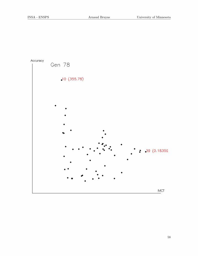
INSA - ENSPS Arnaud Bruyas University of Minnesota
58

INSA - ENSPS Arnaud Bruyas University of Minnesota
E Different set of chromosomes on the first video recorded atthe lab-school, using the second selection method
59

INSA - ENSPS Arnaud Bruyas University of Minnesota
60
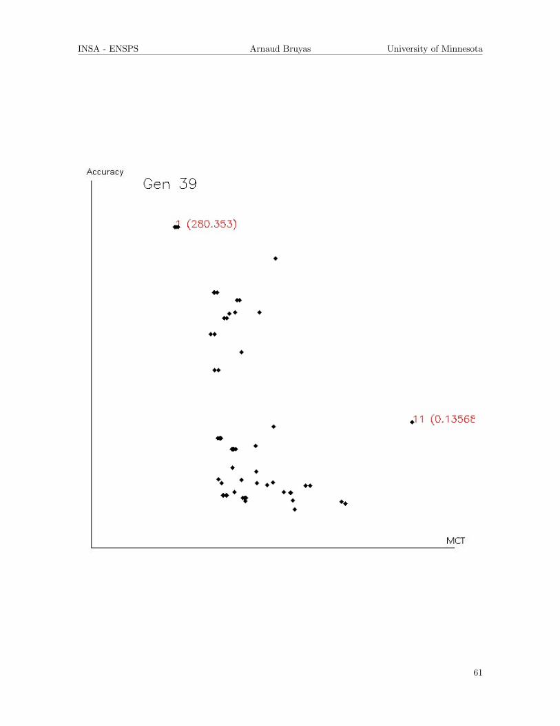
INSA - ENSPS Arnaud Bruyas University of Minnesota
61
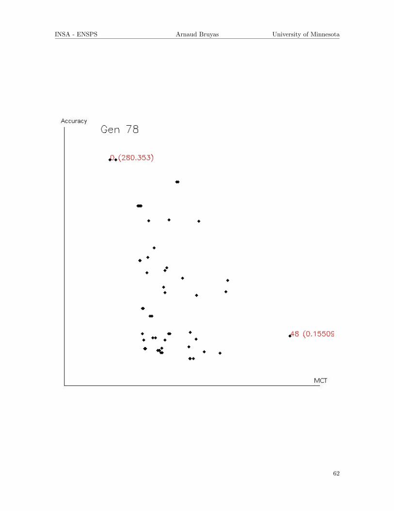
INSA - ENSPS Arnaud Bruyas University of Minnesota
62

INSA - ENSPS Arnaud Bruyas University of Minnesota
F New Scientist article about the project
63

INSA - ENSPS Arnaud Bruyas University of Minnesota
64

INSA - ENSPS Arnaud Bruyas University of Minnesota
G Description of the Center of Distributed Robotics
During this internship, I worked in the Center of Distributed robotics of the University of Minnesota.The major goal of the lab is the creation of robots, from the hardware to the software, but also thedevelopment of algorithms in the vision field.
The first robot developed by the lab was the UMN scout, in partnership with Honeywell, MTSand ATC. It is a two wheel cylindrical robot build for exploration. Nowadays, a company calledRecon Robotics has been founded to sell this robot. It is mainly used by the Army as an explorationdevice. Currently, more than 4000 Scout have been sold, and several improvements have been made tocreate other models, presented on the website (http://distrob.cs.umn.edu). Other mobile robots aredeveloped by the lab, like the Looper or the Adelopod, also presented on the website.
With the development of the Vision and Computer Science field, the lab also started to developalgorithms to monitor human activity (http://mha.cs.umn.edu). The application fields are the mon-itoring of the crowd in public area like train or bus station, but also activity detection and real-timetracking.
The lab is directed by Professor Nikos Papanikolopoulos, helped by Dr Vasilius Morelas, Dr VolkanIsler, Dr Maria Gini and Dr. Stergios Roumeliotis. About 30 graduate students are working in the lab,assisted by 30 undergraduate students. In the end, each professor supervises around 10 to 15 students.Their job is to find grants and projects for the lab and assign each project to the students.
The main outlines of the projects are discussed during brainstorming sessions with all the graduatestudents. But all the achievements and the computer implementations are made by the students. Inthe end, they are very independent. They can manage their day as they want and organise theirschedule as they want. The supervisors are informed only by weekly reports. I really appreciated thisway of studying because of the independence and the trust given by my supervisor.
65

INSA - ENSPS Arnaud Bruyas University of Minnesota
H Working in a laboratory of an American University
Working in an American lab was also part of the experience. I had the opportunity to discover anew way of studying and working.
First, all the students in the lab, stuying for a Master or a PhD, have to take classes. In US, studentscan choose their classes. Even if there are some restrictions, they can build their own curriculum, andtherefore they are more involved in their courses.
Secondly, the lab is part of the University and a lot of teachers are also involved in the researchfield. Thus, they are involving students in the lab by offering them projects to pass their classes. Inthe end, undergrad students are also part of the lab. They can help PhD students in order to maketheir researches easier. In this way, PhD students can work faster, and undergrad students can alsodiscover the research field. It is a way for the teachers to observe the undergrad students in order tooffer them or not a position for a Master in the lab.
For what I have seen, the lab was lead like a company. There are constraints in time and results,since the amounts of money involved are very significant. The grants that the lab is receiving are huge(about several millions of dollars), and in return, the results of the researches have to be consistentand important. Furthermore, someone is employed by the lab in order to find grants and projects forthe lab, but also in order to find real applications for the projects.
Regarding to the work in the lab, each student works on different projects, in order to diversify theirskills and find an area of interest. Therefore, each project is the result of the cooperation of severalstudents. It is very helpful, since ideas are coming from different people, with more or less experiencein the field. As a result, there is a kind of auto-training in the group, which is advantageous for bothstudents and professors. It generates a stimulating atmosphere in the lab.
66

INSA - ENSPS Arnaud Bruyas University of Minnesota
I ICRA 2012 in Saint Paul - Minneapolis: A unique experi-ence
The International Conference on Robotic and Automation is a world-known conference and oneof the most important in the field of Robotic in the world. Each year, the robotic community joinstogether in order to expose different projects and achievements.
Since my supervisor, Mr Papanikolopoulos was the general chair of ICRA 2012, I had to be avolunteer during the event, and therefore, I was able to assist to all the talks and workshops. Itwas an amazing opportunity to see the latest progresses in the robotic field and state of the artprojects developed in many different countries. This concerns many different area of application,such as nanotechnology, medicine, computer science, etc. Over 5 days, Professors and students meettogether to presents their latest achievements and discuss about it in the course of workshops, talksand various sessions. Moreover, this event also exhibits a lot of robotic companies, coming to showtheir latest products and innovations, such as Willow Garage and the PR2 robot, Intuitive Surgicaland the DaVinci chirurgical robot or the NASA and the Robonaut for instance. Hence, it was a greatopportunity for me to see the outcomes of the researches.
This conference was for me extremely impelling and I discovered so many new things that I didn’tthink was possible nowadays in the field of robotics. It motivates me to continue in the research field,and it is one of the reasons that I will start a PhD in Robotic.
Figure 33: Image issued from icra2012.org
67

INSA - ENSPS Arnaud Bruyas University of Minnesota
J ICRA paper
The following paper is only a draft of the article. The one that will be subimitted to the ICRAconference is still in correcting process.
68

INSA - ENSPS Arnaud Bruyas University of Minnesota
References
[1] J. Fasching, N. Walczak, R. Sivalingam, K. Culleny, B. Murphyz, G. Sapirox, V. Morellas, andN. Papanikolopoulos, “Detecting risk-markers in children in a preschool classroom.”
[2] N. Walczak, J. Fasching, W. Toczyski, R. Sivalingam, N. Bird, K. Cullen, V. Morellas, B. Murphy,G. Sapiro, , and N. Papanikolopoulos, “a nonintrusive system for behavioral analysis of childrenusing multiple rgb+depth sensors,” IEEE Workshop on Applications of Computer Vision, jan2012.
[3] R. Sivalingam, A. Cherian, J. Fasching, N. Walczak, N. Bird, V. Morellas, B. Murphy, K. Cullen,K. Lim, G. Sapiro, and N. Papanikolopoulos, “A multi-sensor visual tracking system for behaviormonitoring of at-risk children,” Perceptual and motor skills.
[4] P. Felzenszwalb and D. Huttenlocher, “Efficient graph-based image segmentation,” InternationalJournal of Computer Vision, vol. 59, no. 2, pp. 167–181, 2004.
[5] V. Arsigny, P. Fillard, X. Pennec, and N. Ayache, “Log-euclidean metrics for fast and simplecalculus on diffusion tensors,” Magnetic Resonance in Medicine, vol. 56, pp. 411–421, aug 2006.
[6] G. Esposito and P. Venuti, “Analysis of toddlers’ gait after six months of independent walking toidentify autism: a preliminary study,” Perceptual and motor skills, vol. 106, no. 1, pp. 259–269,2008.
[7] G. Esposito, P. Venuti, F. Apicella, and F. Muratori, “Analysis of unsupported gait in toddlerswith autism,” Brain and Development, vol. 33, no. 5, pp. 367–373, 2011.
[8] X. Zhou, R. Collins, T. Kanade, and P. Metes, “A master-slave system to acquire biometricimagery of humans at distance,” Proceeding IWVS ’03 First ACM SIGMM international workshopon Video surveillance, pp. 113–120, 2003.
[9] J. Yang and A. Waibel, “A real-time face tracker,” Applications of Computer Vision, 1996. WACV’96., Proceedings 3rd IEEE Workshop on, pp. 142–147, dec 1996.
[10] S. N. Sinha and M. Pollefeys, “Pantiltzoom camera calibration and high-resolution mosaic gener-ation,” Computer Vision and Image Understanding, vol. 103, no. 3, pp. 170–183, sept 2006.
[11] A. Senior, A. Hampapur, and M. Lu, “Acquiring multi-scale images by pan-tilt-zoom control andautomatic multi-camera calibration,” Application of Computer Vision, 2005. WACV/MOTIONS’05 Volume 1. Seventh IEEE Workshops on, vol. 1, pp. 443–448, Jan 2005.
[12] R. Hartley and A. Zisserman, Multiple view geometry in computer vision. Cambridge Univ Press,2000.
[13] X. Clady, F. Collange, F. Jurie, and P. Martinet, “Object tracking with a pan-tilt-zoom camera:application to car driving assistance,” Robotics and Automation Magazine, IEEE, vol. 2, pp.1653–1658, 2001.
[14] B. Espiau, “Effect of camera calibration errors on visual servoing in robotics,” ExperimentalRobotics III: Lecture Notes in Control and Information Sciences, vol. 200, pp. 182–192, 1994.
[15] F. Chaumette and S. Hutchinson, “Visual servo control part 1: Basic approaches,” Robotics andAutomation Magazine, IEEE, vol. 13, no. 4, pp. 82–90, dec 2006.
[16] ——, “Visual servo control part 2: Advanced approaches,” IEEE Robotics and Automation Mag-azine, vol. 14, no. 1, pp. 109–118, 2007.
69

INSA - ENSPS Arnaud Bruyas University of Minnesota
[17] S. Stillman, R. Tanawongsuwan, and I. Essa, “A system for tracking and recognizing multiplepeople with multiple cameras,” Georgia Institute of Technology, Tech. Rep. GIT-GVU-98-25,1998.
[18] O. Tuzel, F. Porikli, and P. Meer, “Region covariance: A fast descriptor for detection and classi-fication,” Computer Vision ECCV 2006, vol. 3952, pp. 589–600, 2006.
[19] T. Weise, “Global optimization algorithms: Theory and application,” 2009. [Online]. Available:http://www.it-weise.de/projects/book.pdf
[20] P. Czyzak and A. Jaszkiewicz, “Pareto simulated annealing: A metaheuristic technique formultiple-objective combinatorial optimization,” Journal of Multi-Criteria Decision Analysis,vol. 7, no. 1, pp. 34–47, jan 1998.
[21] A. Konaka, D. W. Coitb, and A. E. Smith, “Multi-objective optimization using genetic algorithms:A tutorial,” Reliability Engineering And System Safety, vol. 91, pp. 992–1007, Sept 2006.
[22] J. Horn, N. Nafpliotis, and D. E. Goldberg, “A niched pareto genetic algorithm for multiobjectiveoptimization,” IEEE World Congress on Computational Intelligence, vol. 1, pp. 82–87, 1994.
[23] E. Zio, P. Baraldi, and N. Pedroni, “Selecting features for nuclear transients classification bymeans of genetic algorithms,” IEEE Transactions on Nuclear Science, vol. 53, pp. 1479–1493,June 2006.
[24] A. E. Eiben, R. Hinterding, and Z. Michalewicz, “Parameter control in genetic algorithm,” IEEETransactions on Evolutionary Computation, vol. 3, no. 2, July 1999.
[25] “Vapix.” [Online]. Available: http://www.axis.com/techsup/cam servers/dev/cam http api index.php
[26] “libcurl.” [Online]. Available: http://curl.haxx.se/libcurl/
[27] “Opencv.” [Online]. Available: http://opencvlibrary.sourceforge.net
[28] A. Cherian, S. Sra, A. Banerjee, and N. Papanikolopoulos, “Efficient similarity search for co-variance matrices via the jensen-bregman logdet divergence,” IEEE International Conference onComputer Vision (ICCV), pp. 2399–2406, 2011.
70