galaxies

Article

Applications of a Particular Four-DimensionalProjective Geometry to Galactic Dynamics

Jacques L. Rubin

Institut de Physique de Nice—UMR7010-UNS-CNRS, Université de Nice Sophia Antipolis,Site Sophia Antipolis, 1361 route des lucioles, 06560 Valbonne, France; jacques.rubin@inphyni.cnrs.fr;Tel.: +33-(0)4-92-96-7323

Received: 25 June 2018; Accepted: 1 August 2018; Published: 3 August 2018

Abstract: Relativistic location systems that extend relativistic positioning systems show thatpseudo-Riemannian space-time geometry is somehow encompassed in a particular four-dimensionalprojective geometry. The resulting geometric structure is then that of a generalized Cartan space(also called Cartan connection space) with projective connection. The result is that locally non-linearactions of projective groups via homographies systematically induce the existence of a particularspace-time foliation independent of any space-time dynamics or solutions of Einstein’s equationsfor example. In this article, we present the consequences of these projective group actions andthis foliation. In particular, it is shown that the particular geometric structure due to this foliationis similar from a certain point of view to that of a black hole but not necessarily based on theexistence of singularities. We also present a modified Newton’s laws invariant with respect tothe homographic transformations induced by this projective geometry. Consequences on galacticdynamics are discussed and fits of galactic rotational velocity curves based on these modificationswhich are independent of any Modified Newtonian Dynamics (MOND) or dark matter theories arepresented.

Keywords: projective geometry; general relativity; relativistic localizing systems; relativisticpositioning systems; rotational velocity curve; hyperbolic space; Newton’s law; black hole

PACS: 04.20.-q; 04.20.Cv; 04.50.-h; 04.50.Kd; 04.80.-y; 04.90.+e; 98.10.+z; 95.30.-k; 95.30.Sf; 98.80.Jk

1. Introduction

In this paper, we present consequences of a local projective geometry of spacetime. This geometryis strongly suggested based on only purely metrological characteristics of systems of relativisticlocalization of events in spacetime [1–3]. The projective theory of relativity differs fundamentallyfrom a conformal theory of relativity, although they both share certain types of scale invariance. In aconformal theory, the local spacetime geometry is Euclidean (and pseudo-Riemannian only once aLorentzian metric is given, restricting the set of admissible changes of coordinates, and an affineconnection) and the changes of scale are due to the additional transformations that allow to passfrom the Poincaré group to the Weyl group. In the projective theory of relativity, the local spacetimegeometry is truly projective and not Euclidean and changes of scale are only invoked when passingfrom homogeneous coordinates of a point of spacetime to its inhomogeneous coordinates whichare its actual spacetime coordinates. In addition, the group of this theory is the five-dimensional,real projective group restricted to one of its projective sub-groups once a Lorentzian metric isgiven. As a result, considering in particular the normal Riemann coordinates that always exist on a(pseudo-)Riemannian manifold, then any change of Riemann normal coordinates attached to a givenfixed point is no longer only linear but can also be homographic. In fact, this geometric structure is that

Galaxies 2018, 6, 83; doi:10.3390/galaxies6030083 www.mdpi.com/journal/galaxies

Galaxies 2018, 6, 83 2 of 26

of a generalized Cartan space (projective Cartan connection space) initially formulated by O. Veblen,B. Hoffmann [4] then mainly by J.A. Schouten [5] among others and then truly conceptualized in allgenerality by C. Ehresmann [6,7] to other geometric structures (Euclidean, affine, conformal, projective,almost complex, affine complex, contact elements).

The three-dimensional projective geometry in spacetime is well-known for velocities which aretransformed by homographies (viz., the relativistic velocity-addition law), but the present projectivegeometry is a four-dimensional projective geometry relating exclusively to events. The projectivetheory of the relativity was mainly investigated during the first half of the 20th century, but it was atthat time impossible to identify the “projective” coordinates (rather called ‘homogeneous’ coordinates)to physical observables. That is certainly one of the reasons why it fell completely into oblivion [4,5].On the other hand, this mathematical theory was itself in full development and there was no realsimple and unified presentation of it; it was puzzle-like yet maturing. The mathematical formalism wasthen presented in a very little synthetic form and difficult to access except for some mathematicians inthe field.

This projective geometry that relativistic localization systems unveil is truly inherent in spacetimeand somehow superimposes itself on the underlying pseudo-Riemannian geometry. In addition, thisprojective geometry is not a consequence only of the localizing processes, otherwise they would haveno connection with spacetime at all. More precisely, quoting A. N. Whitehead (Chap. IX [8]), we can saythat “... something which is measured by a particular measure-system [the latter] may have a special relation tothe phenomenon whose law is being formulated. For example, the gravitational field due to a material object atrest in a certain time-system may be expected to exhibit in its formulation particular reference to spatial andtemporal quantities of that time-system.” This view is in a way the opposite of that of the other greatmathematician D. Hilbert and usually admitted in general relativity, viz. that the physics of spacetimeis somehow independent of its conditions of observations; and yet dependent on this physics.

The objective of this work is to determine the possible effects and geometric constraints imposedby this local projective geometry on the different physical fields, and how this geometry interfereswith relativistic or even classical processes as limit cases. The first question we naturally addressis to determine the types of possible metrics resulting from the transition between homogeneousand inhomogeneous coordinates. We give a result for a particular class of conformal metrics initiallyassociated with the canonical metric defining hyperbolic space. This could be generalized from amore general (−,−,−,−,+) type metric on the initial hyperbolic space. Secondly, an equally naturalapplication is that of possible modifications to Newton’s law of universal gravitation.

The paper is organized as follows. In Section 2, after a brief terminological introduction onthe notions of invariance, equivariance relations and covariance, and how these notions manifestthemselves specifically for tensors in a space with a projective structure, we present how homographiesact. Then, starting from a space-time not temporally oriented initially, and for this reason havinga Euclidean rather than pseudo-Euclidean structure, we identify this space-time to the hyperbolicRiemannian space on which the group of homographies acts transitively. Then, temporally orientingthe spacetime manifold, we can then univocally deduce a pseudo-Riemannian structure startingfrom the hyperbolic Riemannian structure, and that we call “pseudo-hyperbolic” identified withthe pseudo-Riemannian spacetime manifold. As a consequence of this pseudo-hyperbolic structure,only a subgroup of the projective group acts on the spacetime manifold in a non-transitive and notlocally transitive manner. The result is the existence of a particular spacetime foliation that is invariantwith respect to a subgroup of the group of homographies, as well as conformal classes of Lorentzianmetrics that are also invariant. The scalar curves of some of these metrics are given with someother characteristics.

Then, in Section 3, a basic presentation is given of the types of invariant tensors called “projectivetensors” in relation to the group of homographies. There are big differences between some classes ofthese tensors and those of the (pseudo-)Euclidean geometries. The major difference being that they areno longer elements belonging to R-modules but elements of modules defined on fields of homogeneous

Galaxies 2018, 6, 83 3 of 26

fractions of degree 0 in homogeneous coordinates. A particular type of vectors, the simplest, is givenas an example and applied to define modified Newtonian gravitational forces compatible with theprojective structure. A subsection follows on the interpretation of time and distance in relation tothese changes.

In Section 4, examples are given of the possible consequences of these changes in Newton’s law ofgravitation on rotational velocity fields such as those in galaxies. In Section 5, we discuss the particularstructure of the foliation identified and presented in the previous sections. The remarkable thing aboutthis foliation is that it indicates a structure very similar to what a black hole might have. In particular,the spacelike equatorial sphere S2, which is the singular manifold for all the projectively invariantLorentzian metrics, contained in the limit leaf S3 of the foliation could be identified with a so-calledclosed trapped surface of a black hole. We suggest in this section how the possible dynamics of massivebodies could be subjected, in a certain way, to this foliation. These are only preliminary suggestionsfor possible further works. In particular, the role of thermodynamic and/or non-ergodicity ratherthan metric trapping is suggested without further theoretical details. Finally, before concluding, wepresent in Section 6 rotational velocity curve fits for about 10 galaxies. We give details of the procedurefollowed to fit the galactic rotation curves from the possible modified Newton’s laws and the results ofthese fits on a random series of about 10 galaxies. We do not present the successful fits among those ofa larger set of galaxies fits but rather a single sequence of fits for galaxies that were taken at randomamong 175 galaxies in the SPARC database. Successive fits were systematically possible without anycriteria being invoked to select the galaxies other than a possible weak ellipticity.

Besides, we ought to mention Arcidiacono-Fantappié’s theory [9–11]. It is a projective theory ofrelativity constructed from de Sitter’s space. It was also applied by L. Chiatti [12] to produce fits ofgalaxies in good agreement with the observations. Nevertheless, the projective aspect of this theory istotally different and far removed from the historical mathematical approach of projective geometryapplied to relativity due to Veblen et al. and Schouten et al. In the present article, the proposedmodifications of Newton’s law are directly derived from homographic invariance and the spaceconsidered is not de Sitter’s space. In addition, in the Arcidiacono-Fantappié theory, the homogeneouscoordinates are directly the space-time coordinates with an additional coordinate which is not thecase in our approach. In this, we tried to follow as much as possible the historical approach of theAmerican and Dutch mathematics schools which historically mathematically conceptualized projectivedifferential geometry and its application to relativity. To quote Wojnar et al. [13], we obtain a muchsimpler and in our opinion more mathematically justified modification of Newton’s law.

Finally, we conclude in the last section in which we indicate in particular other motivations thatled to the publication of this note.

2. The Projective Structure

2.1. Some Elements of Terminology

In this first section, we first specify some terminology used throughout the article. To be brief,we will not present the rigorous mathematical definition of the well-known notion of equivarianceof invariant tensors but only how it manifests itself in the case of projective geometry. It differsnaturally and strongly from the notion of covariance which essentially expresses that a given geometricobject is covariant or contravariant if it is a tensor for the geometry considered. Many examples ofsuch equivariance of invariant tensors can be given, such as those whose components are sphericalharmonics associated with irreducible representations of the group of rotations. More generally, wehave this notion of equivariance for special functions or, equivalently, right-invariance of tensor fields

Galaxies 2018, 6, 83 4 of 26

defined on fibers of fiber bundles with respect to their structural groups. More precisely, in the case ofspherical harmonics Ym′

` (r), they are transformed under the action of a rotationR as follows:

Ym` (R

−1. r) =`

∑m′=−`

D(`)mm′(R)Ym′

` (r) (1)

where D(`)mm′(R) is an element of the Wigner matrix D(`)(R). Then, they define an SO(3)-invarianttensor field Y`(r) with values in R`. Then, equivariance only means that the components of the tensorfield Y`(r) satisfy the relations of equivariance (1) with respect to SO(3). Hence, an invariant tensorfield is said to have equivariant components. In the same context, a non-invariant tensor field T`(r)would be such that Tm

` (R−1. r) ≠ Sm` (R−1. r) ≡ ∑

`m′=−` D(`)mm′(R) Tm′

` (r), i.e., its components do notsatisfy the relations of equivariance although it remains covariant; in other words, its componentsare transformed linearly with respect to rotations and therefore it is indeed a tensor. In the case ofprojective invariance, we would have similar linear relations but in which the rotations R actinglinearly on r would be replaced by homographies acting on coordinates by birational transformationsgeneralizing the so-called Möbius transformations.

2.2. The Homographies on Projective Space

To fix the ideas on these homographies, we start from the following geometric situation. LetM bea four-dimensional differential manifold considered as the no-time oriented, time orientable spacetimemanifold, and A a maximal atlas onM constituted by systems of local coordinates ui (i = 1, . . . , 4)on the open sets of chart in A. Let U ⊂ M be one of these open sets and e any point in U. Then,we denote by Ve ⊂ U one of the open neighborhoods of e containing the point p ∈ Ve of coordinates ui

p.Among the local coordinates that can be considered are the Riemann normal coordinates attached tothe event e. Then, these Riemann normal coordinates ui are considered to be inhomogeneous coordinatescorresponding to the homogeneous coordinates Uα (α = 0, . . . , 4) such that ui ≡ Ui/Uα0 where α0 ∈

1, . . . , 4 is fixed and obviously Uα0 ≠ 0. In everything that follows, we will consider essentially andonly the case α0 ≡ 0. Then, let A ≡ (Aα

β) be an element of G ≡ GL(R, 5). In addition, we denote by AA

the sub-matrix of A such that AA ≡ (Aij).1 Then, the coordinates Uα are transformed by A into the new

homogeneous coordinates U′α as follows:

⎧⎪⎪⎪⎨⎪⎪⎪⎩

U′0 = A00 U0 +A0

j U j,

U′i = Ai0 U0 +Ai

j U j.(2)

The inhomogeneous coordinates ui are then obviously transformed into the new inhomogeneouscoordinates u′i by birational transformations [A] (homographies) such that u′ = [A](u), i.e., we have

u′ = [A](u) ∶ u′i =Ai

0 +Aij uj

A00 +A

0j uj . (3)

More generally, the group of such homographies [A] is the projective group PGL(5,R) = SL(5,R)

which acts transitively on the quotient homogeneous space G/G = RP4 of points (ui) where G is theparabolic subgroup of linear transformations A. The latter define the so-called (general) homologies[A] keeping fixed the origin e of coordinates ui

e = 0 (i.e., Ue ≡ (U0e , 0, 0, 0, 0) whatever U0

e ≠ 0 is). Thus,any matrix A ∈ G is such that Ai

0 = 0. In addition, the no-time oriented spacetime manifold is then locally

1 We shall throughout this paper adhere to the convention that Greek suffixes shall take on values from 0 to 4 and Latinsuffixes only the values 1 to 4.

Galaxies 2018, 6, 83 5 of 26

homeomorphic in a particular way to the hyperbolic space H4 ⊂ RP4 of which the definition we recallis the following.

2.3. The Hyperbolic and “Pseudo-Hyperbolic” Spaces

Let the non-degenerate quadratic form Q on R5 be such that Q(U) = (U0)2 −∑4i=1(Ui)2 and the

corresponding pseudo-Euclidean metric ds2 = ∑4i=1(dUi)2 − (dU0)2. In addition, let the canonical

projecting map π be such that π ∶ (Uα) ∈ R5 − 0Ð→ (ui) ∈ RP4 with, as a particular case, ui = Ui/U0

whenever U0 ≠ 0. Furthermore, we denote by Ω ⊂ RP4 the open set of lines in R5 generated by Usuch that Q(U) > 0.2 The variety Ω is homeomorphic to R4 noting besides that the cell-decompositionof RP4 is RP4 = R4 ∪RP3. Thus, we have also RP4 ≃ Ω ∪RP3. Then, Ω equipped with the metricds2 restricted to the submanifold Z of elements U such that Q(U) = 1 and U0 > 0 defines a (notpseudo-)Riemannian analytic submanifold of RP4 called hyperbolic space H4 ≡ (Ω, ds2/Z).

It is important to note that the projective space RP4 is the space of lines in R5 passing throughthe origin and that the lines in π−1(Ω) intersect the variety Z into a single point only thus univocally

representing a point of the projective space. More precisely, let U be such that U0 =√

1+∑4i=1(Ui)2 ≡

S(Ui), i.e., π(U) ∈ Ω and U ∈ Z. Then, the Euclidean metric ds2H ≡ ds2/Z defined on H4 is the pull-back

σ∗(ds2) of ds2 by the section σ ∶ u = (ui)Ð→ (S(ui), u) and then we obtain

ds2H =

∑4i=1(dui)2 +∑

4i=1<j(uj dui − ui duj)2

1+∑4i=1(ui)2

. (4)

In particular, we deduce also that det(ds2H) = (1 +∑4

i=1(ui)2)−1. The metric ds2H is a Euclidean

metric which is invariant, like H4, with respect to the restricted Lorentz group SO+(1, 4) ⊂ PGL(5,R)

of homographies. In addition, SO+(1, 4) acts transitively on H4. Hence, locally, we have also RP4 ≃

H4 ∪RP3.We could have started from a more general situation with a metric on hyperbolic space of the

(−,−,−,−,+) type. We consider in the whole article only the standard case at first for simplicity’s sake.Other metric classes could of course be considered later. The most general situation would have beento start with a metric ds2 of the form

ds2≡

4∑

α,β=0καβ(U) dUα dUβ, (5)

where the coefficients καβ(U) would have been homogeneous functions of degree 0 in the variables Uµ.The hyperbolic space H4 is a simply connected manifold contrarily to the not simply connected

anti-de Sitter spaces which therefore cannot be ascribed to R4 ≡ Ω ≃M. One may object that this wouldnot allow to define a Lorentzian metric onM. However, first, the metric ds2

H is only deduced from thedefinition of H4 itself defined from the quadratic form Q and notM. Second, we can easily define aLorentzian metric dτ2 onM from ds2

H onceM is time oriented, i.e., if there exists a nowhere vanishingvector field ξ0 onM ascribed to a cosmological time. Indeed, let ω0 be the differential 1-form onMdual to ξ0, i.e., such that ω0(ξ0) = 1, then it can be shown [14] that the metric

dτ2≡ 2 ω0 ⊗ω0 − ds2

H (6)

2 It is important to note for the continuation that the hyperbolic space is not the whole set of points u ∈ R4 such that thereexists a point U ∈ R4 such that u = π(U) and Q(U) > 0. This means that the hyperbolic space is not the image by sections µof π, i.e., such that π µ = id; although maps can be defined from the hyperbolic space to R5.

Galaxies 2018, 6, 83 6 of 26

is a Lorentzian metric whenever 0 < dτ2(ξ0, ξ0) < 2, i.e., whenever ξ0 is time-like. We can choose forinstance ω0 ≡ du1. Then, we obtain a Lorentzian metric such that

det(dτ2) = −

1+ 2 (u1)2

1+∑4i=1(ui)2

, (7)

and which is the Minkowski metric at the origin e ≡ (uie = 0) of the system of Riemann normal

coordinates. Moreover, this new metric dτ2 is the pull-back by σ (equivalently, the restriction to Z) ofthe pseudo-Euclidean metric

ds2≡ (dU0

)2+ (dU1

)2−

4∑i=2

(dUi)

2 (8)

which is invariant with respect to the pseudo-orthogonal group O(2, 3) associated with the quadraticform Q(U) ≡ (U0)2 + (U1)2 −∑

4i=2(Ui)2. Thus, because dτ2 is a pull-back by σ then dτ2 is defined on

the whole of Ω.

Definition 1. Let Q be a non-degenerate quadratic form on R5 and P one of the connected sets of points U ∈ R5

such that Q(U) = c (c = cst). In addition, let ρ be a homeomorphism from Ω to P and a subgroup K ⊆ GL(5,R)

keeping invariant Q. By action via ρ or ρ-action of a subgroup K ⊆ GL(5,R), we mean that if AA ∶PÐ→P isthe linear isometric action relative to Q of any A ∈ K on P, then the ρ-action of the subgroup [K] ⊆ PGL(5,R)

of homographies on Ω is defined by the homeomorphism JAKρ ≡ ρ−1 AA ρ ≡ Ad [ρ](AA). Furthermore,we agree to omit the index ρ whenever ρ ≡ σ or P ≡ Z.

Definition 2. Let V ⊂ Ω be a subset in Ω and A an element in GL(5,R). Then, the definition domainof homography [A] is ΩA ≡ Ω − HA where HA is the empty set or an affine hyperplane of codimension 1(i.e., the ‘singularities hyperplane’). Then, we denote also by VA the subset such that VA = V −HA for any givenset V ⊆ Ω.

Lemma 1. Let A be any element in R∗ × SO+(1, 4) and the four-dimensional open ball B4 ⊂ Ω and ∂B

4= S3.

Then, we have B4∩ HA = ∅, [A](B4) = B4, [A](S3) = S3 and [A](ΩA − B

4) = ΩA−1 − B

4.

Proof. From the definition of Z, we get first π(Z) = B4 ⊂ Ω. In addition, from the definition of[A] we have [A] π = π A. Then, because R∗ × SO+

(1, 4) keeps invariant the quadratic form Qand acts transitively on Z then the group of homographies SO+

(1, 4) acts also transitively on theopen ball B4. As a result, that means that the hyperplanes HA associated to each homography[A] ∈ SO+

(1, 4) are outside the open ball B4, i.e., B4 ∩ HA = ∅. Then, we deduce with B4 that[A](B4) = [A] (π(Z)) = π(AZ) = π(kA Z) = π(Z) = B4 where kA ∈ R∗. Also, because [A] and [A]−1 arecontinuous bijective maps on B4 there are both open-closed maps on B4.

Second, let A be any given element in R∗ × SO+(1, 4). Then, HA is the set of elements (ui) ∈ Ω

such that (I): ∑4i=1 A

0i ui +A0

0 = 0. Moreover, from the definition of R∗ × SO+(1, 4) we have necessarily

(II): Q(A0) ≡ (A00)

2 −∑4i=1(A

0i )

2 = ±µ2 where µ ≠ 0. Hence, because B4 ∩ HA = ∅ then if B4∩ HA ≠ ∅

there exists only a unique point such that u0 ≡ (ui0) ∈ S3 = ∂B4 in B

4∩ HA. Then, HA is the tangent

space of S3 at u0. Therefore, necessarily, there exists λ ≠ 0 such that (III): A0i = λ ui

0 with (IV):∑

4i=1(ui

0)2 = 1. It is then easy to show that there does not exist µ ≠ 0 such that all the conditions

(I), (II), (III) and (IV) are satisfied. Then, because [A] and [A]−1 are continuous on ΩA ∩ΩA−1 and

bijective maps then there are open-closed maps on ΩA ∩ ΩA−1 ⊃ B4. As a result, since we have

[A](B4) = B4 ⊆ [A](B4) ⊆ [A](B4) = B

4and [A] is a closed map on ΩA ∩ΩA−1 so that [A](B

4) is closed,

then B4⊆ [A](B

4) ⊆ B

4from which we deduce that [A](B

4) = B

4and then [A](S3) = S3. In addition,

because [A] and [A]−1 are continuous bijective maps on B4

there are both open-closed maps on B4.

Galaxies 2018, 6, 83 7 of 26

Third, because [A]−1 is defined on set [A](ΩA − B4) = [A](ΩA) − B

4⊆ Ω − B

4and not on HA−1 ,

then [A]−1 is defined on [A](ΩA − B4) = [A](ΩA)− B

4⊆ ΩA−1 − B

4. Hence, we have [A](ΩA − B

4) ⊆

ΩA−1 − B4

and similarly [A]−1(ΩA−1 − B4) ⊆ ΩA − B

4.

Property 1. Let ρ be a differentiable bijective map from Ω to Z and aρ the embedding (i.e., injective immersion)from Ω to the four-dimensional open ball B4 ⊂ Ω such that aρ ≡ π ρ. In full generality, aρ differs from identity.Then, we have aρ JAKρ = [A] aρ for any A ∈ R∗ × SO+

(1, 4).

Proof. Indeed, we have by definition [A] π = π A and JAKρ = ρ−1 AA ρ. Thus, we obtainaρ JAKρ = π AA ρ = [AA]π ρ = [A]π ρ = [A]aρ. Moreover, aρ is an embedding (not invertiblein full generality) from Ω to B4 because the restriction π/Z of π to Z is an injective immersion (to Ω ≃ R4)between manifolds of same dimensions and π(Z) = B4 ⊂ Ω.

Property 2. If ρ is a diffeomorphism then so is aρ.

Proof. The map π/Z from which the inverse of aρ can be defined as invertible. Indeed, let u be a pointin Ω, then the point U ≡ π−1

/Z(u) ∈ Z is such that Ui = U0 ui with Q(U) = 1 and U0 ⩾ 1. Therefore,

we deduce that U0 = 1/√

1−∑4i=1(ui)2 and therefore π−1

/Z is well defined and differentiable for any

u ∈ B4. Furthermore, as a result, it is a diffeomorphim between Z and B4.

As a result, the metric dτ2 remains invariant with respect to a ρ-action of the group SO+(2, 3) ⊂PGL(5,R) = SL(5,R) of homographies deduced from the quadratic form Q of the anti de Sitter spaceAdS4 ≡P ⊂ R5; the latter being defined by the relation Q(U) = s2 > 0 where s = cst. Indeed, formally,we obtain for any A ∈ R∗ ×O(2, 3): JAK∗ρ(dτ2) = (AA ρ)∗ ρ−1∗(dτ2) = ρ∗ A∗A(ds2) = ρ∗(ds2) = dτ2.However, the morphim ρ ∶ V ⊆ Ω Ð→ Ads4 cannot be defined globally on Ω and, moreover, in order toremain on the domain space Ω and Z defined from the quadratic form Q, we must rather consider thesubgroup [G+

τ ] ≡ SO+(2, 3)∩ SO+(1, 4) ⊂ PGL(5,R) only where G+τ ⊂ GL(5,R) acts linearly on R5 via

ρ ≡ σ and which is a non-compact group containing O(1, 3); the latter acting on the coordinates Uα forα = 0, 2, 3, 4. In addition, the homographic action of [G+

τ ] via σ and especially not via any section of π

on Ω is neither transitive nor even locally transitive as shown below.

2.4. The Foliations

Definition 3. Let K be a subgroup of GL(5,R). Then, we call π-orbits of [K] ∈ PGL(5,R) the orbits in PR4

defined from the homographic actions of homographies [A] where A ∈ K.

Let the quadratic form Q be such that Q(U) ≡ Q(U) + 2(U1)2 where Q(U) > 0. Then, we havealso Q(U) > 0. Moreover, the quadratic forms Q and Q are invariant with respect to G+

τ up to sameconformal factors; hence their ratio Q/Q which is defined on R4 ≃ Ω from the projecting map π.More precisely, we have Q(U)/Q(U) = 1 + 2(U1)2/Q(U) ≡ π∗(q(u)) = q π(U) ≡ k = cst ⩾ 1 whereu = π(U) which is invariant with respect to [G+

τ ]. Therefore, the π-orbits of [G+τ ] are subsets of points

u ∈ Ω such that q(u) = k. Note that we have q([A](u)) = q(u) for any A ∈ G+τ . Indeed, we have

π∗(q(u)) = q π(U) and, in addition, u′ = [A](u) = [A] π(U) = π(AU) where u = π(U). Hence, weobtain π∗(q(u′)) = π∗(q([A](u))) = q π(AU) = Q(AU)/Q(AU) = π∗(q(u)).

Then, two cases are deduced depending on whether k = 1 or k > 1:

• If k > 1, then, necessarily, U1 ≠ 0 and consequently from q(u) = k we obtain: α2 (u1)2+∑4i=2(ui)2 = 1

with u1 ≠ 0 where α2 ≡ (k + 1)/(k − 1) > 1, and• if k = 1, then 1) U1 = 0 and therefore u1 = 0 whatever the ui’s are for i = 2, 3, 4, or 2) Q(U) = +∞

and necessarily U0 = +∞ and ui = 0 for i = 1, . . . , 4.

Therefore, we obtain also that

Galaxies 2018, 6, 83 8 of 26

• u ∈ 0×R3 ≡ E0,3 whenever k = 1, and• u ∈ S3

α − E0,3 if k > 1 where S3α is a three-dimensional ellipsoid.

In addition, as a result, the π-orbits of [G+τ ] are subsets in the ellipsoids S3

α or E0,3.Note that a point u ∈ Ω is an element of an ellipsoid S3

α if and only if u ∈ B4 where B4 is theopen ball of points u such that ∑4

k=1(uk)2 < 1. In addition, the equatorial sphere S2 ⊂ E0,3 such that

∑4k=2(uk)2 = 1 and u1 = 0 is the common intersection in S3 = ∂B

4of ellipsoids S3

α.

Property 3. Let p be the function defined on Ω such that p ≡ q a = a∗(q) where a = π σ ∶ Ω Ð→ B4. Then,we have p(JAK(u)) = p(u) for any A ∈ G+

τ and p(u) = 1+ 2 (u1)2.

Proof. First, we can note that the definition domain Dq of q(u) ≡ 1 + 2 (u1)2/(1 −∑4k=1(uk)2) is Dq =

(Ω − S3)∪ E0,3. Then, from the definition of p and Property 1, we have q(a JAK(u)) = q([A] a(u)) =q(a(u)). Moreover, we obtain p(u) = 1+ 2 (u1)2 from a direct computation with a ∶ (ui) ∈ Ω Ð→ (vi) ∈

B4 ⊂ Dq where vi ≡ ui/√

1+∑4k=1(uk)2.

Remark 1. Then, from Property 3, we obtain if q(u) = k that p(u) = a∗(q)(u) = k = (α2 + 1)/(α2 − 1) ⩾ 1.

Definition 4. We call σ-orbits in Ω the orbits of [G+τ ] via σ and thus defined from the actions JAK of elements

A ∈ G+τ .

Theorem 1. The π-orbits of [G+τ ] in B4 ⊂ Ω are the three-dimensional, disjoint, simply connected and connected

sets H3+α , H3−

α and B3 ∩ E0,3 where H3+α (resp. H3−

α ) is the north (resp. south) hemisphere of S3α, i.e., the set of

points u ∈ S3α such that u1 > 0 (resp. u1 < 0). Note that B3 ∩ E0,3 is the limit case in B4 of H3±

α whenever α

tends to infinity. Then, we denote by H3∞ the leaf such that H3∞ ≡ B3 ∩ E0,3.

Proof. Let u be a point in H3±α . Then, because π/Z is a diffeomorphism between B4 and Z there exists a

unique point U ∈ Z such that π(U) = u. From the algebraic definition of S3α and the quadratic form Q

we find that U is necessarily such that (U1)2 = 1/(α2 − 1). Hence, the set of points U = π−1/Z(u) where

u ∈ H3±α are elements of the hyperboloid defined by equation (U0)2 −∑

4i=2(Ui)2 = α2/(α2 − 1). However,

G+τ ∩ SL(5,R) acts transitively on this hyperboloid. Thus, [G+

τ ] acts transitively on any H3±α . It is the

same for B3 ∩ E0,3 since it is the limit case α2/(α2 − 1)→ 1 whenever α →∞.

Corollary 1. The σ-orbits of [G+τ ] in Ω relative to the representation J K are the spacelike hyperplanes Hε

ksuch that p(u) = k ⩾ 1 and sgn(u1) = ε. Moreover, we have JAK∗(dτ2) = dτ2 on Ω for any A ∈ G+

τ and eachH±k is diffeomorphic to the leaf H3±

α such that k = (α2 + 1)/(α2 − 1).

Proof. These assertions come simply from the fact that map a ≡ π σ is a diffeomorphism and fromTheorem 1.

Corollary 2. Let O ≡ H3±α , 1 < ∣α∣ ⩽ +∞ be the topological leaf space of π-orbits (leaves) H3±

α in B4. Then,

the leaf space O is a Hausdorff space of which the leaves are not separated by closed neighborhoods on B4.

Moreover, the π-foliation on B4 is open, connected, transversally oriented (by ∣α∣− 1 ∈ R+∗) and saturated in B4.

Proof. Indeed, we have B4 = ⋃+∞∣α∣=1 H3±

α and [G+τ ] operates continuously on B4 via the representation

[ ]. Then, for the leaf space O ≡ B4/[G+τ ] to be Hausdorff, it is necessary and sufficient (§8, I.52 Prop. 1,

I.55 Prop. 8 [15]) that the graph set (u, u′) ∈ B4 × B4 /u′ = [g]. u, [g] ∈ [G+τ ] of the continuous action

of [G+τ ] is closed in B4 × B4, i.e., that each orbit H3±

α is closed; what they are on B4. Now, these leaves

H3±α are neither open nor closed in B

4since any neighborhood (in the topology on B

4induced by that

of Ω) in B4

of point u0 in the equatorial 2-sphere S2 ⊂ S3 = ∂B4

intersects all the leaves H3±α . Then the

latter are not separated by closed neighborhoods in B4. On the contrary, there would exist two closed

Galaxies 2018, 6, 83 9 of 26

neighborhoods U3±α of H3±

α and U3±α′ of H3±

α′ such that U3±α and U3±

α′ are disjoint. However, all such

closed neighborhoods contain the adherences H3±α that intersect in S2.

Moreover, we have the following inversions:

• the inversion between H3+α and H3−

α is obtained by the u1-time inversion T ∶ (u1, ui)Ð→ (−u1, ui)

(where i = 2, 3, 4),• the space inversion P ∶ u ≡ (u1, ui)Ð→ (u1,−ui) (where i = 2, 3, 4) on each leaf H3±

α , and• the inversion I in the 3-sphere S3 that is the map I ∶ (ui) ∈ B

4∗Ð→ (ui/R2) ∈ Ω − B4 where

R2 ≡ ∑4j=1(uj)2.

We can characterize more the matrices A of the group G+τ . They must preserve the two quadratic

forms Q and Q up to a same conformal factor. For this last reason, this implies that Q −Q and Q +Qare also preserved up to same conformal factors. Consequently, the spaces U1 = 0 and U0 = U2 = U3 =

U4 = 0 are proper spaces and the matrices A are then completely reducible. They are matrices suchthat A1

α = Aα1 = 0 whenever α ≠ 1 and A1

1 ≠ 0. In addition, their first minors, obtained by deleting thesecond raws and second columns associated with the coordinate U1 are elements of R∗ ×O(1, 3). Notethat the group O(1, 3) acts in two distinct ways on inhomogeneous coordinates: by homographiesand as invariance subgroup of the quadratic forms Q and Q, and linearly as invariance group of theLorentzian metric dτ2.

Furthermore, we restrict the group G to the subgroup G+τ ≡ G+

τ ∩G of which the matrices A ∈ G+τ

have their coefficients A0i and Ai

0 for i = 2, 3, 4 vanishing. Hence, considering the restriction to(0, 0)×R3 of the action of G+

τ , then G+τ restricts to the group R∗ ×O(3). Moreover, [G+

τ ] is the groupof (general) homologies preserving the origin e of the system of Riemann normal coordinates (note thatall homologies leaving variable fixed points do not form a group). Then, the coset space [G+

τ /G+τ ] is

the sub-group of elations (special homologies) preserving the origin e to which corresponds the groupG+

τ /G+τ of boosts analogous only to those in relativity.

Definition 5. We call “pseudo-hyperbolic space” H1,3 the pseudo-Riemannian manifold Ω equipped with theLorentzian metric dτ2.

We can note that this pseudo-Riemannian space H1,3 is neither a anti-de Sitter space nor any ofits projections on a particular projective space. In fact, we are in an unusual situation in which wehave the Euclidean space R5 on which is defined the metric ds2 which is the one used to define thenon-simply connected anti-de Sitter space AdS4, but we are not using the pull-back which defines thisspace as a variety of dimension 4; namely the pull-back by a section like the section (ui) ∈ R4 Ð→

(U0 =

√

1+∑42(ui)2 − (u1)2, Ui = ui) ∈ R5. In fact, we use the section σ resulting from the definition of

hyperbolic space H4 which is simply connected and advantageous from the topological point of viewto return to the entire simply connected space R4 specific to Riemann normal coordinates. The priceto pay is a non-transitive action of invariance groups and the existence of a foliation on R4. Thisis a disadvantage from the point of view of group actions but this disadvantage could turn into anadvantage in physics as we will see later.

In other words, there is a kind of competition between the pseudo-Riemannian structure on oneside and the projective structure on the other and, metaphorically, there is a kind of “peace agreement”along the leaves only.

In addition, we define the coefficients gij(u) such that

dτ2≡

4∑

i,j=1gij(u) dui duj. (9)

Galaxies 2018, 6, 83 10 of 26

Thus, we obtain⎧⎪⎪⎪⎪⎪⎪⎪⎪⎪⎪⎪⎪⎨⎪⎪⎪⎪⎪⎪⎪⎪⎪⎪⎪⎪⎩

g11 = 1+(u1)2

χ(u)2 ,

gii =(ui)2

χ(u)2 − 1, (i ≠ 1)

gij =ui uj

χ(u)2 , (i ≠ j)

(10)

where χ(u)2 ≡ 1 +∑4i=1(ui)2. Then, in particular, we obtain from dτ2 its determinant and the

non-negative scalar curvature Sc such that

det(dτ2) = −

(1+ 2 (u1)2)

χ(u)2 , Sc =12 (u1)2

(2 (u1)2 + 1)2 . (11)

Hence, our approach differs from those usually considered in general relativity with anti-de Sitterspaces. Then, it suffices to restrict the group of homographies to the group [G+

τ ] ⊂ SL(5,R) = PGL(5,R)

compatible with the invariance of the Lorentzian metric dτ2 on the σ-orbits of [G+τ ].

Finally, we give the following definition of a projective geometric object.

Definition 6. A geometric object, e.g., a tensor, is said projectively invariant if it is invariant with respect to[G+

τ ] on all σ-orbits of [G+τ ] in H1,3. It is said to be partially projectively invariant if it is invariant with respect

to a proper subgroup of [G+τ ].

In particular, a geometric object on the union Ω of σ-orbits, can be non-continuous on Ω butcontinuous only when restricted to any spacelike leaf H±k , i.e., we consider the case where only thediscrete topology on Ω with respect to the σ-foliation remains.

2.5. A Particular Discontinuous Projectively Invariant Lorentzian Metric

We have shown the map a ∶ Ω Ð→ B4 is a diffeomorphism and its inverse a−1 ∶ (ui) ∈ B4 Ð→ (u′i) ∈Ω is defined by the relations u′i ≡ a−1(u)i = ui/

√

1−∑4k=1(uk)2. Then, the metric dh2 ≡ a−1∗(dτ2)

defined on B4 is continuous and projectively invariant along each leaf H3±α with respect to the

group [G+τ ] with the representation [ ]. Indeed, from relation a JAK = [A] a, we deduce that

[A]∗(dh2) = [A]∗ a−1∗(dτ2) = a−1∗ JAK∗(dτ2) = a−1∗(dτ2) = dh2. However, dh2 is necessarily not

continuous on the equatorial sphere S2 ⊂ S3 = ∂B4

because the leaves H3±α cannot be separated by

closed neighborhoods on B4

and, more specifically, on any neigbhourhood of the spacelike equatorialsphere S2 ⊂ E0,3. Then, considering the inversion I in the 3-sphere S3, we define dh2 ≡ I−1∗(dh2) on

Ω − B4

which is therefore no more continuous on S2 but also projectively invariant along each leaf

I(H3±α ) ⊂ Ω − B

4with respect to the group [G+

τ ] with again the representation [ ]. Besides, we can

note that I(H3∞) = E0,3 − H3∞. Indeed, I commutes with [ ], i.e., for all A we have [A] I = I [A].

Then, Ω − S3 equipped with the metric dh2 ≡ (dh2, dh2) on (Ω − B4) × B4 is a Lorentzian metric that

diverges to infinity on S3; which can be shown by a direct calculation using a symbolic calculationsoftware (SCS). In addition, we find that dh2 is the Minkowski metric at u = 0, i.e., at the event e originof the Riemann normal coordinates. We can say that dh2 is topologically singular on S3. Furthermore,

we obtain a π-foliation and a representation [ ] of [G+τ ] which extend from B4 to Ω− B

4via inversion I.

A natural way to get around this singularity problem on S3 is to consider a class of conformalmetrics dν2 ≡ Ψ2(u) dh2 defined from dh2 and suitable functions Ψ. The latter must be invariant withrespect to [G+

τ ] with representation [ ] to preserve the π-foliation. Hence, Ψ must be a function Ξ(q)

Galaxies 2018, 6, 83 11 of 26

of the fraction q(u) from which the leaves were deduced. Besides, a direct computations using a SCSshows that the determinant of dh2 and its scalar curvature Sc are such that

det(dh2) = −

(R2 + 1)2((R2 − 1)2 + 2 (u1)2)

((R2 − 1)2 + R2)(R2 − 1)10 ≡

K(u)(R − 1)10 ,

Sc =12 (u1)2 (R2 − 1)2

((R2 − 1)2 + 2 (u1)2),

(12)

where R2 = ∑4k=1(uk)2 and K is then such that ∣K(u)∣ < +∞ on B

4. In addition, the metric dh2 is the

Minkowski metric at u ≡ 0. Therefore, from the algebraic expression for q(u) which is of the form

(u1)2/(1− R) in the vicinity of R = 1, to obtain a metric dν2 with a finite determinant on B4, then the

function Ξ must be such that

Ξ(q) ≡C(q)q5/4 , (13)

where C(q) is a continuous function, bounded on [1, +∞[ and such that C(+∞) = c∞ ≠ 0 wheneveru1 ≠ 0. Moreover, if ∣C(1)∣ = 1 then dν2 is the Minkowski metric at u = 0. Unfortunately, the finitenessof det(dν2) cannot be maintained if u1 = 0 and R ≠ 0, i.e., on the equatorial sphere S2 ⊂ E0,3. Hence,

the metric dν2 is defined on B4− S2 and we define dν2 ≡ I−1∗(dν2) on Ω − (B4 ∪ S2). Then, we define

the following particular pseudo-Riemanniann manifold.

Definition 7. We call “singular pseudo-hyperbolic space” H1,3s the pseudo-Riemannian manifold Ω equipped

with the Lorentzian metric dν2 ≡ (dν2, dν2) topologically singular on S2.

We then discuss in Section 5 a possible relationship between this singular pseudo-hyperbolicspace H1,3

s and the admissible metrics in black hole theory.In addition, we can say that the open ball B4 is equipped with an orbifold structure by considering

the finite group Γ having inversion I as generator. Then, we have B4 ≡ H1,3s /Γ.

3. The Invariant Tensors with Respect to Homographies

3.1. Introduction—Invariance of Families of Tensors or Tensors Fields

So far only one system of Riemann normal coordinates explicitly attached to point e has beenconsidered. The singular metrics dh2 or dν2 (resp. dτ2) are metric fields defined on the space Ωalso attached to this point. We have shown that these fields of metrics are invariant with respectto the group [G+

τ ] of homographies with representation [ ] (resp. J K). These fields therefore havecomponents that are equivariant with respect to this same group, i.e., we typically have relations suchas ωij([A].u) ≡ Mk

i (u)Mhj (u)ωkh(u) for their components ω and for any element A ∈ G+

τ where thematrices M such that detM ≠ 0 are the Jacobian matrices univocally defined from the homographies[A] (resp. JAK).

Now, if we consider the particular case of a force as the gravitational force, the latter is attached toa point, the “source” point e in this case, and it applies to another mass at a “target” point p ∈ Ω. Ofcourse, this is not a force field on Ω. Indeed, we can perfectly have a second mass at another target pointp′ and therefore we have a second gravitational force always attached to the single source point e. Sowe have a family of gravitational forces all attached to the same source point e. The fact that the generalmathematical expression of gravitational forces does not change according to the selected variabletarget point p means that we have a particular invariance of this family. It is therefore somehow agravitational force attached to the single source point e that is a field because parameterized by theselected target point p ∈ Ω but not a force field on Ω giving in that case only, a force vector attached toeach source point in Ω. This may seem unusual, but it is clear experimentally that several different

Galaxies 2018, 6, 83 12 of 26

forces can be applied to a mass. That only the single total applied force is considered does not changethe fact that originally several distinct forces apply, each associated with different target points p.This is especially true since the general formula for this single total force will not take the generalmathematical form of the different forces of which it is made up.

Naturally, the group of invariance that must be considered is the group [G+τ ] in order to define

this family of forces at e as a projective geometric object. In addition, this family will be associatedwith a family of equivariant components with respect to this same group applied on the set of targetpoints p ∈ Ω. Thereafter, choosing a particular force in this family, this force vector will be used insome way as a germ at the source point e to infer a particular force fields class defined on the spacetimemanifoldM. In what follows, we will focus only on the invariance of these force families with respectto group [G+

τ ] with representation [ ] attached to the single origin source point e ∈M.

3.2. Invariant Families of Tensors Attached to a Single, Given Point

Now, the objective is to determine invariant vectors with respect to [G+τ ] and representation [ ]

(from which invariance relative to representation J K is deduced with the map a) in order to determinea modification of Newton’s law compatible with the projective structure. However, the Newtonianforce being a 3-vector, only a group isomorphic to the group of rotations SO(3,R) will be considered.Hence, only the stronger invariance with respect to the group [G+

τ ] of homologies must be considered.In particular, the latter keeps conformally invariant the time dependent Euclidean spatial metric

d ˆ2=

4∑

i,j=2γij(u) dui duj, (14)

where γij ≡ ω1j ω1i/ω11 − ωij (i, j = 2, 3, 4) and ωαβ are the components of the metric dh2 defined in B4.Using a SCS, we find that

det(d ˆ2) =

(R2 + 1)2((R2 − 1)2 + 2 (u1)2)

(R2 − 1)6D(R, u1)

, (15)

where

D(R, u1) = R8

− (8 (u1)

2+ 3) R6

+ (8 (u1)

4+ 13 (u1

)2+ 4) R4

− (8 (u1)

4+ 10 (u1

)2+ 3) R2

+ 8 (u1)

4+ 5 (u1

)2+ 1, (16)

where R2 ≡ ∑4j=1(uj)2. Moreover, if u2 = u3 = u4 = 0 and (u1)2 < 1 then we obtain in particular:

d ˆ2≡

1

((u1)2 − 1)2

4∑k=2

d(uk)

2. (17)

It can be shown by direct numerical computations that D(R, u1) > 0 whenever R2 < 1 and (u1)2 < 1.Hence, det(d ˆ2) is positive in B4. In addition, its scalar curvature S` is of the form:

S`(R, u1) ≡

N(R, u1)

(R2 + 1)3((R2 − 1)2 + 2 (u1)2), (18)

where N(R, u1) is a polynomial with relative integer coefficients and of degree 14 with respect to Rand of degree 8 with respect to u1. Numerical computations again show that N(R, u1) is negativewhenever R < 1 and (u1)2 < 1 and vanishes for R = 1 and u1 = 0. In addition, we obtain N(R =

1, u1) = 768 (u1)6 ((u1)2 − 1) and thus S`(R = 1, u1) ≡ 48 (u1)4 ((u1)2 − 1) meaning, in particular, that S`

Galaxies 2018, 6, 83 13 of 26

vanishes on the spacelike equatorial sphere S2. Using inversion I, we deduce its counterpart d ˇ2 on

Ω − B4

from dh2 with also a negative scalar curvature since the inversion I is a conformal map. Hence,

S` is negative or null and bounded on B4. In addition, that the metric d ˆ2 is invariant with respect to

O(3) is well known. Its conformal invariance with respect to [G+τ ] comes simply from the fact that G+

τ

is isomorphic to (R∗)3 ×O(3) and that the three scale factors belonging to (R∗)3 are distinct in fullgenerality.

Now, we can define projective families of vectors attached to source origin point e as [G+τ ]-invariant

vector fields with respect to target points p starting from the following general framework.

3.2.1. General Framework for Invariant Projective Vector Fields

The general results presented in this paragraph are well known and are standard constructions.We present them briefly nevertheless to fix the ideas and the notations, and to indicate very elementarybut essential properties which will be used in part in the continuation. The fundamental and technicalaspects are related to the theory of moduli spaces of projective invariants [16,17] and projectiveschemes [18].

Let V be a vector field on R5 such as V(U) ∈ R5 for U ≡ (Uα) ∈ R5 given. Then, if we considerformulas (2) and setting V(U)α ≡ Uα, then V is naturally invariant with respect to GL(5,R) sincewe have V(AU) ≡ A V(U) whatever is A ∈ GL(5,R). Then, V(U) is an element of the fiber overU in the so-called tautological bundle over the base space R5. Thus, any vector field Wn such thatWn(U) ≡ V1(U)⊗⋯⊗ Vn(U) where each Vi is a copy of V, i.e., Vi ≡ V, is also invariant with respect toGL(5,R). As a result, for some indices n ∈ I ⊂ N∗, any analytical vector field IWn which is an irreduciblepart of Wn in R5 with respect to GL(5,R) is also invariant with respect to GL(5,R) and, moreover, itscomponents are homogeneous polynomials of degree n in the variables Uα.

We can generate an other class of invariant vector fields given any fixed element A0 ∈

GL(5,R) in full generality. The matrix A0 can depend in its definition on a set k of N arbitraryparameters k1, k2, . . . , kN independent of the points U unlike the most general matrices A which haveonly numerical fixed coefficients. Or, if nevertheless A0 depends on the points U, we consider itscoefficients as homogeneous functions of degree 0 to keep the homogeneity degrees of the componentsof the vectors involved in the various relations of equivariance. That also means that they can dependonly on the inhomogeneous coordinates ui.

In other words, we consider that the whole set of GL(5,R)-invariant vector fields is a finiteK0-module where K0 is the function field of homogeneous functions of degree zero with respect tovariables Uα.

Then, defining Z such that Z(U) ≡ A0 V(U) with A0 independent of U, we obtain for anyA ∈ GL(5,R) the relation of equivariance Z(AU) = ιA0(A) Z(U) where ιA0 is the inner automorphismassociated with A0, i.e., ιA0(A) ≡ A0 AA−1

0 . In addition, if A0(U) has coefficients that are homogeneousfunctions of degree 0 with respect to the variables Uα, then we obtain also a relation of equivarianceZ(AU) = ι∗A0

(A) Z(U) where ι∗A0(A) ≡ A0(AU)AA−1

0 (U) is homogeneous of degree 0. We refer to

these two cases denoting ι(∗).Then, in the same way as for vectors IWn, for some q ∈ I ⊂ N∗, we can obtain GL(5,R)-invariant,

analytical vector fields IZq on R5.In addition, we can obtain from W and Z analytical vector fields IW

r (U) and IZs (U) on R5,

with values in R4, irreducible with respect to the group GL(4,R). Their equivariance relations are thenIW

r (AU) = AA IWr (U) and IZ

s (AU) = ι(∗)AA0

(AA) IZs (U) for some indices r, s ∈ K ⊂ N∗ and where

A ∈ R∗ ×GL(4,R).Besides, if we project V onto V ≡ (Vi), we deduce also for p, m ∈ J ⊂ N∗, analytical invariant vector

fields IWm ≡ (IWim) and IZp ≡ (IZi

p) on R4 with values this time in R4 and irreducible with respect to

GL(4,R) such that IWm(AA u) = AA IWm(u) and IZp(AA u) = ι(∗)AA0

(AA) IZp(u) where u ≡ (ui) ∈ R4.

Galaxies 2018, 6, 83 14 of 26

To summarize, we have the following list of analytical GL(5,R)-invariant and GL(4,R)-invariantvector fields:

IWn (n ∈ I) ∶ IWn(AU) = A IWn(U),

IZq (q ∈ I) ∶ IZq(AU) = ι(∗)A0

(A) IZq(U),

IWr (r ∈ K) ∶ IW

r (AU) = AA IWr (U),

IZs (s ∈ K) ∶ IZ

s (AU) = ι(∗)AA0

(AA) IZs (U),

IWm (m ∈ J) ∶ IWm(AA u) = AA IWm(u),

IZp (p ∈ J) ∶ IZp(AA u) = ι(∗)AA0

(AA) IZp(u).

(19)

3.2.2. Invariant Projective Vector Fields on Ω

Previous vector fields are not vector fields on Ω except for vector fields IWm and IZp but theycan be nevertheless projectable on this space. For, we can consider the push-forward Kn = (Ki

n) of

the projectable, non-analytical vector field ( IWin/ IW

0n)i=1,...,4, of which the components are homogeneous

fractions of degree 0 with respect to the variables Uα, by the projecting map π, i.e., Kn(u) ≡

π∗ ( IWin/ IW

0n)(u). Then, the vector field Kn on H1,3

s is invariant with respect to homographies

[A] ∈ [G+τ ] only, i.e., we have

Kn([A](u)) = AA(u)Kn(u) (20)

where AA ≡ λA AA with λA a real scaling function is a frame field on H1,3s defined from A.

In the same way, we can define non-analytical, invariant vector fields Hq(u) ≡ π∗ ( IZiq/ IZ

0q)(u)

which satisfy the relations of equivariance

Hq([A](u)) = ι(∗)A0

(AA)(u) Hq(u) (21)

with respect to [G+τ ] only.

Similarly, the following analytical vectors on H1,3s are defined:

In ≡ π∗( IWn) (n ∈ I) ∶ In([A](u)) = A In(u),

Jq ≡ π∗( IZq) (q ∈ I) ∶ Jq([A](u)) = ι(∗)A0

(A) Jq(u),

Ir ≡ π∗(IWr ) (r ∈ K) ∶ Ir ([A](u)) = AA Ir (u),

Js ≡ π∗(IZs ) (s ∈ K) ∶ Js ([A](u)) = ι

(∗)AA0

(AA) Js (u).

(22)

These vectors are invariant with respect to GL(5,R). In addition, we set Im ≡ IWm and Jp ≡ IZp

which are GL(4,R)-invariant analytical vectors.Then, fields of conformally invariant polynomials or polynomial fractions on H1,3

s can bededuced associated with the groups [G+

τ ], [G+τ ] and G+4

τ ≡ GL(4,R)⋂G+τ (notation: conf. invts =

“conformally invariants”) :

[Gτ] = dν2

e (X, Y) / X, Y = Ir or Js , [G+τ ]-conf. invts,

[Gτ] = dνe(X, Y) / X, Y = Kn, Hq, Ir , or Js , [G+τ ]-conf. invts,

Gτ = dνe(X, Y) / X, Y = Im, Jp, Kn, Hq, Ir , or Js , G+4τ -conf. invts,

[G`] = d ˆe2(X, Y) / X, Y = Kn, Hq, Ir , or Js , [G+τ ]-conf. invts,

G` = d ˆe(X, Y) / X, Y = Im, Jp, Kn, Hq, Ir , or Js , G+4τ -conf. invts.

(23)

Note that dνe and d ˆe are, respectively, the Minkowski metric and the spatial canonical Euclideanmetric at e ≡ (ui = 0).

Galaxies 2018, 6, 83 15 of 26

These fields will be of great importance within this framework of projective geometry because itwill be the fields of functions onto which modified Newton’s forces will be defined.

3.3. A Particular Modified Newton’s Law

We can present an example of fractions deduced from the vector field H1 associated with thelinear map A0(k, U) such that

A0(k) =

⎛⎜⎜⎜⎜⎜⎜⎜⎝

a00(k, U) a0

1(k, U) a02(k, U) a0

3(k, U) a04(k, U)

0 1 0 0 00 0 1 0 00 0 0 1 00 0 0 0 1

⎞⎟⎟⎟⎟⎟⎟⎟⎠

, (24)

where a00(k, U)U0 ≠ 0,∑4

i=1 a0i (k, U)ui ≠ 0, k is a set of parameters and the functions a0

α are homogeneousfunctions of degree 0 with respect to the variables Uβ. Then, we obtain after the push-forwards by π:

H1(u) =1

(c0(k, u)+∑4i=1 ci(k, u)ui)

⎛⎜⎜⎜⎜⎝

u1

u2

u3

u4

⎞⎟⎟⎟⎟⎠

, (25)

where a0α ≡ cα. Therefore, from (17) at e, we deduce the the fraction in [G`]:

d2(u, k) =

∑4i=2(ui)2

(c0(k, u)+∑4i=1 ci(k, u)ui)

2 . (26)

Then, setting u1 ≡ t, u2 ≡ x, u3 ≡ y, u4 ≡ z, c1 ≡ ct(k, u), c2 ≡ cx(k, u), c3 ≡ cy(k, u), c4 ≡ cz(k, u) andr2 ≡ ∑

4i=2(ui)2 we obtain the fraction

d2(t, x, y, z) =

r2

(c0 + ct t + cx x + cy y + cz z)2 . (27)

Then, we deduce the modified Newton’s law#„F a/b invariant with respect to [G+

τ ]:

#„F a/b = Gma mb

(c0 + ct t + cx x + cy y + cz z)2

r2#„v , (28)

where G is the universal gravitational constant and #„v is the unit vector directed along the line joiningthe positions of the two punctual masses ma and mb.

We focus mainly on two particular classes of modified Newton’s laws, the first called “isotropic”class, and the other, naturally, “anisotropic” class.

3.3.1. The Isotropic Class

In this case, we want a force invariant with respect to rotations which is the most natural way tochange Newton’s law in a first approach. This also makes it possible to compare these modificationswith others already proposed such as those resulting from MOND theories for example. Thus,we can set for instance c0(k, u) ≡ k0 ≠ 0, ct(k, u) ≡ kt, cx(k, u) ≡ − kx r/x, cy(k, u) ≡ − ky r/y andcz(k, u) ≡ − kz r/z where the k’s are constant or depend only on the time t and radius r. These c

Galaxies 2018, 6, 83 16 of 26

functions clearly originate from homogeneous functions aα of degree 0 with respect to the variablesUα. Then, we obtain

#„F a/b = Gma mb

(k0 + kt t − k r)2

r2#„v , (29)

where k ≡ kx + ky + kz.

3.3.2. The Anisotropic Class

Out of curiosity, we also consider this case of a modified Newton’s law not invariant with respectto rotations, but nevertheless remaining conformally invariant with respect to [G+

τ ]. This case may seemirrelevant to consider given what we know about Newton’s force. However, in fact, some anisotropyof the modified Newton’s force could perhaps provide one of the causes to the shape of galaxies,and more particularly the fact that nearly two thirds of spiral galaxies are barred. The existence ofthese bars could be one of the signatures indicating some form of anisotropy in the causes that governthe dynamics of spiral galaxies. However, we also found an additional characteristic quite unexpectedat first sight and surprising, not related to the existence of the bars, which motivates in a certain waymore strongly the presentation of this singular case in the next sections.

Then, we simply set the functions c to be only constants k0, kt, kx, ky and kz and then we obtainthe following formula for the modified, anisotropic Newton force

#„∖Γ :

#„∖Γ a/b = Gma mb

(k0 + kt t − kx x − ky y − kz z)2

r2 v. (30)

3.4. Interpretation of Times and Distances

Common to these two classes, the time variable t in these modified laws must be interpretedcorrectly on the base of the following remarks. First, it must be independent of the radius r. Therefore,considering that these forces are those exerted by the mass ma on masses mb located at variabledistances rb ≡ r, then t does not vary when r varies. In other words, t is a variable independent of rand common to any mass mb whatever its distance from ma. Second, these values of t and r are thoseevaluated respective to the event e which is the origin event of the Riemann normal coordinates system(ui) used previously. However, it seems difficult to understand that this force varies according to atime of observation of the positions of the masses mb.

This means then that this time t cannot be a time of observation. In fact, it is deduced fromthe time orientation of the spacetime manifoldMmade when choosing the differential 1-form ω0 todefine the Lorentzian metric dτ2 from ds2

H . Then, this variable t, initially associated with u1 in ourexample, should actually be the variation of the cosmological time τC that we will finally note byt ≡ ∆τC. Conversely, observers’ times are given by “non-cosmological” clocks and they consequentlydiffer from ∆τC. Therefore, compared to the times of observers, the modified Newton’s laws varyslowly and can be considered constant in a first approximation.

However, if the variable τC is assigned a cosmological content, then the relative distance rmust also be cosmological, i.e., r ≡ rC. This would mean there are three nowhere vanishing spacevector fields defined everywhere on the spacetime manifold M. This is topologically perfectlyfeasible sinceM is homeomorphic to H1,3 (or H1,3

s ) unlike the anti-de Sitter spaces. However, this isprecisely the Newtonian view of observers who attribute to certain relative distances r an absolutecontent independent of the observer or a cosmological content with “cosmological” rulers to evaluatedistances (e.g., with for instance the Hubble constant, approaches using baryon acoustic oscillations; or,possibly more effective, relativistic localizing systems which extend the galactic, relativistic positioningsystems [19,20] recently implemented by an experiment on board the ISS using X-rays detectionemitted from pulsars [21]).

Therefore, since then the relative distance r ≡ rC between the two masses ma and mb must beinterpreted as a relative cosmological distance, and if we consider for example that these masses are

Galaxies 2018, 6, 83 17 of 26

inside a given galaxy, then rC is related to the relative distance ro (obtained for example by the parallaxmethod) observed by any observer by a function depending on the relative cosmological distance rG

Cof the galaxy. Then, similarly, as a first approximation, we can consider that in the case of galaxiesobservations, rC and ro are proportional, i.e., rC ≡ µ(rG

C , ∆τGC ) ro, and that the different constants in the

modified Newton formulas depend on the cosmological time ∆τGC at which the galaxy is observed and

its cosmological distance rGC from the observers.

Then, from now and throughout the paper, we consider r to be actually the relative distance ro

between the punctual masses observed by observers and t a constant, and the different constants inthe modified Newton’s laws depending only on the considered, observed galaxy.

4. Modified Newton’s Laws

4.1. The Modified, Isotropic Newton’s Law

Now, with this interpretation of the time variable t and considering that k0 + kt t ≡ α is constant,then we obtain:

#„F a/b(r) = Gma mb

(α + β r)2

r2#„v . (31)

Moreover, if we consider the case where α is vanishing, then we obtain also the formula

#„F a/b(r) = Gma mb β2 #„v , (32)

which seems at first sight incoherent. Surprisingly, one of the fits presented later could be in accordancewith this odd case.

Now, we consider that the fraction (27) is also the modified distance between the two masses whichmust be substituted to the distance r. Indeed, this fraction is obtained from the Euclidean metricd`2. Therefore, the centripetal acceleration modulus a must also be modified and must therefore bewritten as

a(r) = ∣α + β r∣v2

r, (33)

where v is the rotational velocity at distance r. Then, considering an infinite disk with mass densityρ(r) at r and assuming that the mass density is a projective invariant, we deduce that the mass M(r)enclosed in a disk of radius r is, up to a multiplicative constant, such that M(r) ≡ ∫

r0 s ρ(s) ds. Then,

up to a multiplicative constant, we deduce that the velocity function with respect to r is such that

v(r) ≡

√

∣α + β r∣M(r)

r. (34)

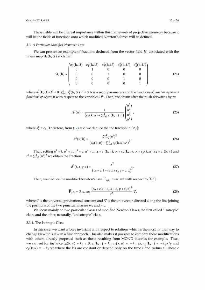
Taking, for instance, the values α = 1 and β = 0.1 with a mass density ρ(r) ≡ ρ1(r) = 1 if r ⩽ 1 and 0otherwise, then we obtain the following figures (see Figure 1) for v(r):

Figure 1. Case with ρ1, α = 1 and β = 0.1: the middle figure is a zoom view from above of the peakvisible on the left figure. The figure on the right is the figure in the middle seen from below.

Galaxies 2018, 6, 83 18 of 26

4.2. The Modified Anisotropic Newton’s Law

Following a similar reasoning to the previous isotropic case, we then obtain the following modifiedanisotropic Newton’s laws:

#„∖Γ a/b(r, φ) = Gma mb

(α + β r cos(φ))2

r2#„v (35)

and#„∖Γ a/b(r, φ) = Gma mb (β cos(φ))

2 #„v , (36)

where φ is the angle between a given reference (possibly “slowly” rotating) line passing through ma

and the line joining ma and mb. In addition, we deduce that

v(r, φ) ≡

√

∣α + β r cos(φ)∣M(r)

r. (37)

Taking, as previously in the isotropic case, the values α = 1 and β = 0.1 with a mass density ρ suchas ρ(r) ≡ ρ2(r) = exp(−r) then we obtain the following but smooth similar surfaces (see Figure 2) forv(r, φ):

Figure 2. Same as Figure 1 but with anisotropic Newton’s law and with ρ2.

Now, with α = 0 and β = 1, we also have with ρ1 (Figure 3) the symmetrical surfaces:

Figure 3. Same as Figure 1 but with anisotropic Newton’s law and with α = 0 and β = 1.

As can be seen from these examples, there is an area close to the center where rotational velocitiesare rapidly variable and both the lowest and almost zero at a central point surrounded by the highestvelocities. These two examples show an interest in these modified Newton’s laws if we relate theexistence of this central zone (some kind of “cyclone’s eye”) to the observed behavior of rotationalvelocities at the center of some galaxies. Now, if we want in particular to know the evolution of thevelocities with respect to the radius only, we compute the mean value of the velocity fields with respect

Galaxies 2018, 6, 83 19 of 26

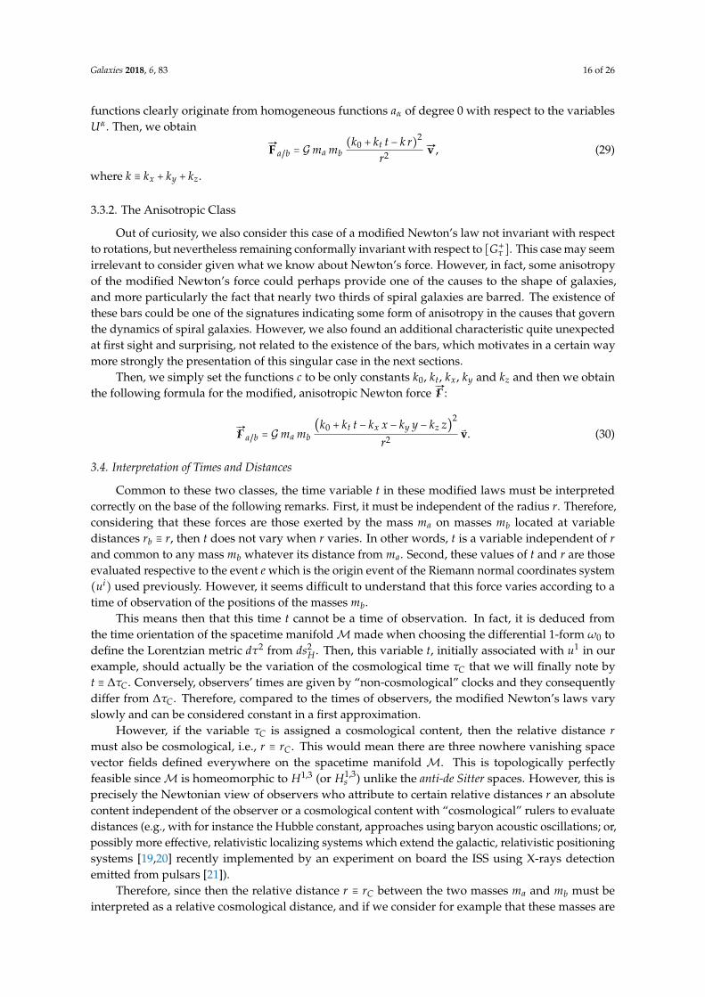
to the angle only. Then, with α = 1 and β = 0.1, we obtain the following variations (Figure 4) withrespect to the radius where <v>(r) ≡ 1

2π ∫2π

0 r v(r, φ) dφ:

Figure 4. Blue curve from ρ1, and red dashed curve from ρ2. Both curves with α = 1 and β = 0.1.

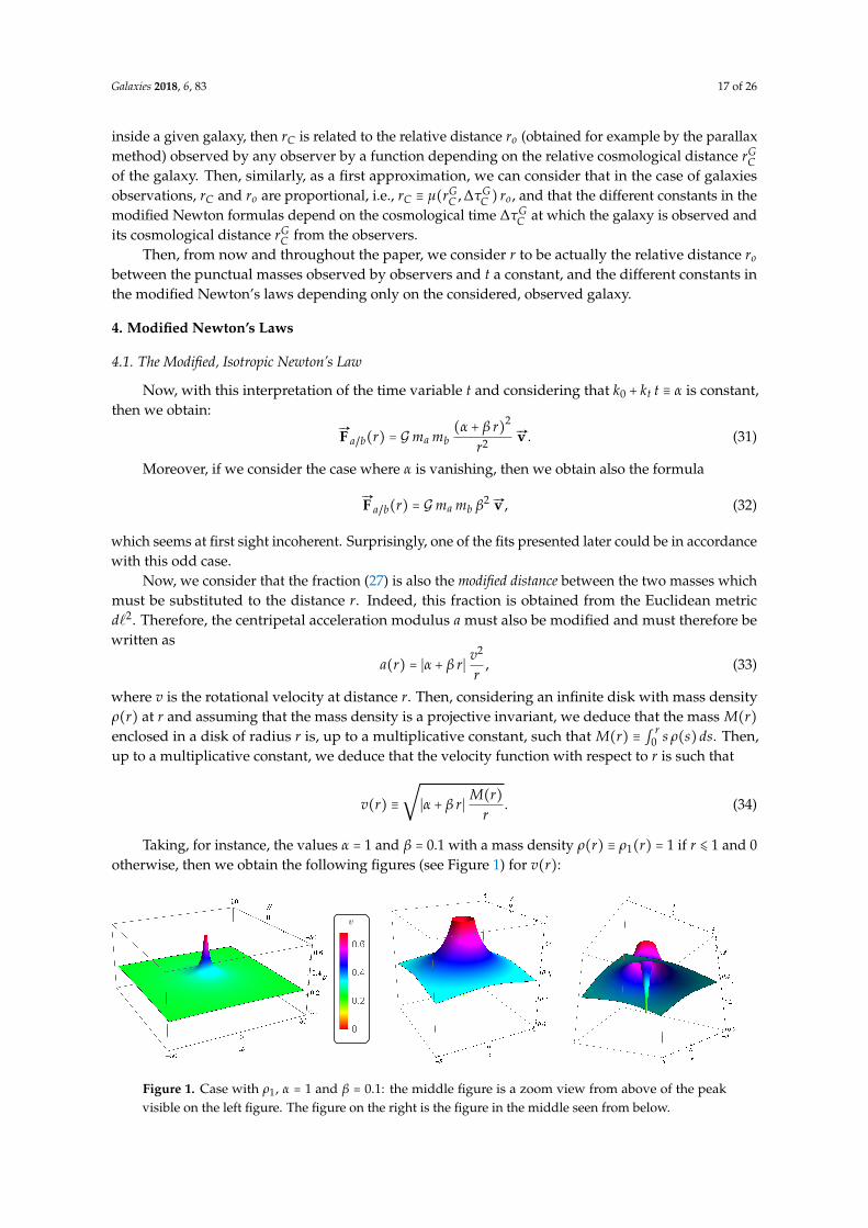
5. The “Central Zone” and a Structure Similar to a Black Hole

The previous figures indicating the rotational velocity fields were performed in a classical frame.However, naturally, as far as galaxies are concerned, the masses at stake need to take into account therelativistic effects whose consequences cannot manifest themselves in these figures. In this case, thismeans that the velocity fields of massive bodies will be subjected to the π-foliation O (Figure 5) if thesebodies are submitted to force fields invariant in addition with respect to [G+

τ ] with representation [ ].

Figure 5. Leaf space in spacetime and π-foliation O. Black disc: open ball B3.

This property with the leaves not ‘separated by closed neighborhoods’ on B4

or on the adherenceof its complementary and the spacelike equatorial sphere S2 (considered as a so-called closed trappedsurface) strongly suggest a particular structure very similar to that of the central black holes (of galaxiesin particular) (Chapter 8 [22]). Indeed, we obtain some of the very fundamental criteria to be satisfiedto obtain such black hole structure, even if some are not such as the singularity on S2 of the metric dh2

for instance contrarily to dν2. Besides, these metrics have no central punctual singularities contrarilyto Schwarzschild metric for instance. The various possible dynamics subjected to this structure

Galaxies 2018, 6, 83 20 of 26

might then be less the result of a particular metric as in black holes theory but rather of a loss ofergodicity or thermodynamic causes. Note that the Hawking-Penrose theorems [23,24] might not beapplicable within the present context with dynamics constrained by homographic invariance and theimplicit Cartan connexion space structure; the latter conceptualized in full general by Ehresmann andinvoked in black hole theory to address the problem of “b-completeness” via Schmidt’s construction(Chapter 8 [22]). These should modify space-time dynamics and/or the types of solutions to beconsidered from Einstein’s equations or their variants in other types of space-time geometrical theories.Moreover, the present black hole-like structure is not fully based on a spacetime dynamics but onlyon the ground, underlying projective geometry and foliation.Hence, we consider a flow of particlesdue to application of modified Newton’s laws of gravitation, the latter being the restricted spatialG+4

τ -conformally invariant parts of force 4-vectors. As a result, the particles would flow towards orfrom an “active center,” namely, the spacelike open ball B3 ⊂ E0,3.

We have seen that the spatial metric d`2 = (d ˇ2, d ˆ2) determines a negative curvature (vanishingon the equatorial sphere S2) and that as a consequence shock waves in fluids could exist. The existenceof such shock waves is proven in astrophysics such as so-called bow shocks for instance. However, herewe would be in the presence of a very particular case in which the shock wave front would be sphericalon a sphere corresponding to the equatorial sphere S2 and perhaps specifically stabilized in a sphericalshape because of the homographic foliation/invariance. However, several phenomena can then occurvery specific to the particular shape of the shock wave front because it is a spatially closed surface.

First of all, if the flow of particles goes from the outside towards the inside of this sphere,the crossing of the shock front is accompanied by an increase in entropy (inside shock fronts, entropycannot be decreased but can increase or not [25]). Moreover, the leaf space O of open π-orbits is theunion of leaves not separated by closed neighborhoods so that a loss of ergodicity is possible in avicinity of this sphere. The loss of ergodicity would also be enhanced from the negative curvatureof the spatial metrics d`2 which we know since Anosov’s works that it reinforces the instability ofgeodesic flows. They would reflect in some way mathematically a stochastic redistribution of dynamicson the equatorial sphere. In other words, we would have a branching process on the equatorial spherebut without rules and which would be the expression of a sudden increase, associated with the shockfront, of the dimension of the unstable submanifold of an Anosov flow. Unfortunately, to the author’sknowledge, there do not seem to be any studies on the ergodic/non-ergodic properties of “singular”Asonov flows with branching or not in four-dimensional manifolds.

This evokes the theory of sonic black holes but with the difference that massive or non particlescan perfectly circulate from the inside to the outside. On the other hand, particles remain particles andare not metaphorically associated with sound waves. Moreover, the fluid is assimilated in the theoryof sonic black holes to a kind of space-time ether whereas here it would rather be a flow circulatingbetween the leaves H3±

α which constrain it as if they were the walls of a nozzle. Metaphorically,we could say that we have a fluid in a supersonic nozzle with a shock wave at the bottleneck.

The thermodynamic consequences would then be as follows. The system beingthermodynamically closed and somehow isolated precisely because of the spherical shape of theshock front, no thermodynamic sources or sinks allow a fluid enclosed by this sphere to decrease itsentropy and then, eventually, to cross against the current the barrier constituted by the shock front.In addition, any non-massive particles (produced by the thermalization of the particles inside the holeas they slow down) that could nevertheless move from inside to outside the sphere would be trappedby the radiative interactions with the non-ergodic entering fluid in a vicinity of the sphere. One canimagine for this a trapping process such as that encountered in Anderson’s diffusion for example withthe difference nevertheless that the diffusion medium has a non-ergodic behavior. However, aftera certain threshold of radiative energy density, some of these non-massive particles could suddenlyescape as lightning bolts and produce a phenomenon similar to that of the firewall on the equatorialsphere. This turbulent dynamic behavior could be similar to the one suggested by Hawking [26].

Galaxies 2018, 6, 83 21 of 26

Thus, such a scenario in such a thermodynamically closed structure would resemble the behaviorof a black hole whose origin would be weakly but not completely related to the spacetime metric.Such a description would therefore suggest that black holes could be some kinds of entropic/ergodicconfining traps produced by a closed surface in the vicinity of which physical processes would bethermodynamically irreversible and/or non-ergodic.

6. The Fits of Rotational Velocity Curves and the Fitting Procedure

In the case of the curve fits we present (Figures 6–12), the point e will always be attached to apoint in space that will be the “center” of the galaxy. Furthermore, the possible constants determiningthe modified Newton’s laws will therefore be dependent only on the galaxy considered and on theobserver who collected the data.

As a result, the intensities FM of the modified Newton’s laws of gravitation have the followinggeneral form up to a multiplicative constant (r ≡ (x, y, z)):

FM(r) ≡ m M(r)(

c0(r)+ cx(r) x + cy(r) y + cz(r) zr

)

2

, (38)

where M(r) is the mass enclosed in a disk of radius r and the functions c depend on ∆τGC and rG

C .It should be noted that this modification nevertheless preserves the action/reaction principle contrarilyto the modifications given in MOND theories [27].

We use the isotropic Formula (34) to make the fits and observational data provided by the SPARCdatabase [28,29] with explanations of how the surface brightness densities are obtained from theARCHANGEL software [30]. Actually, we used two sort of files directly available online on theSPARC database website, namely, the Bulge-Disk Decompositions files ‘XXXXXX.dens’ and the MassModels files ‘XXXXXX_rotmond.dat’ all grouped together and stored respectively in the zip filesBulgeDiskDec_LTG.zip and Rotmod_LTG.zip.

Then, from the ‘XXXXXX.dens’ files, we have the surface brightness densities SBdisk andSBbulge of, respectively, the disks and the bulges of the galaxies XXXXXX with respect to the radius.These densities are also partially given in the files ‘XXXXXX_rotmond.dat’ but these files give lesspoints/data to make good fits. Therefore, we use in ‘XXXXXX_rotmond.dat’ files only the rotationalvelocity values Vobs with their error bars errV as functions of the radius Rad, i.e., the variable r.

In addition, we consider that the mass M(r) is given, up to a multiplicative constant, by theformula (Frederico Lelli; private communication):

M(r) ≡ ∫r

0[SBdisk(x)+ SBbulge(x)] x dx. (39)

This formula is based on the assumption that (1) the disks of the galaxies with their possiblebulges have negligible thicknesses with respect to their diameters, and (2) that the circularity defect(circular symmetry of the disks) is negligible except perhaps for extremely elliptical galaxies. Therefore,this integral is the integral of a density on a disk of radius r up to the multiplicative constant 2π

coming from the integration on the polar angle. Then, given a galaxy XXXXXX, we apply the followingsequence to produce the fit of the rotational velocity Vobs with respect to the radius r:

(i) We make a fit of the total surface brightness density SB(r) = SBdisk(r)+ SBbulge(r). Typically,the functions used to make the fit are sums of functions such as p(r) eq(r) or u(r)/w(r) where p(r),q(r), u(r) and w(r) are polynomials.

(ii) We compute the integral (39) as a function of the primitive functions of the functions used in step (i)to make the SB fits. In other words, we compute M(r) as the primitive function of the SB function.

(iii) Then, we fit the model functions M(r) to experimental data Vobs(r)2, i.e., we seek for constants α

and β which minimize the least-square errors defined from the following differences:

Galaxies 2018, 6, 83 22 of 26

Vobs(r)2−

(α + β r)r

M(r). (40)

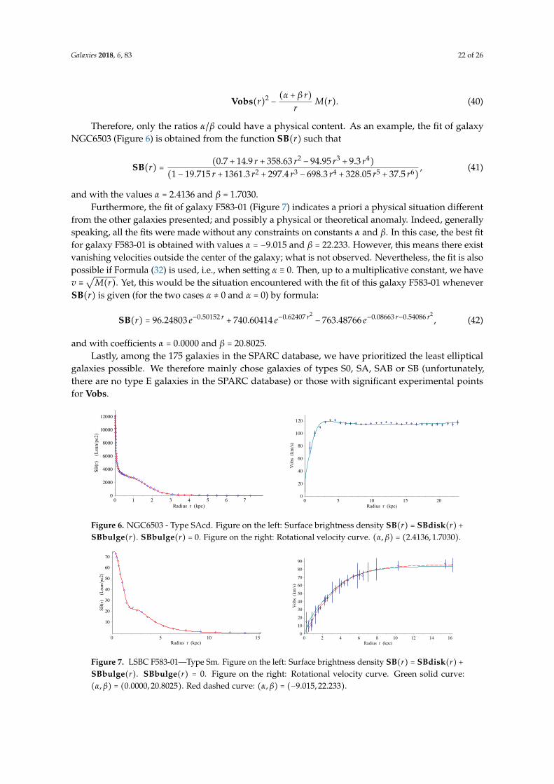
Therefore, only the ratios α/β could have a physical content. As an example, the fit of galaxyNGC6503 (Figure 6) is obtained from the function SB(r) such that

SB(r) =(0.7+ 14.9 r + 358.63 r2 − 94.95 r3 + 9.3 r4)

(1− 19.715 r + 1361.3 r2 + 297.4 r3 − 698.3 r4 + 328.05 r5 + 37.5 r6), (41)

and with the values α = 2.4136 and β = 1.7030.Furthermore, the fit of galaxy F583-01 (Figure 7) indicates a priori a physical situation different

from the other galaxies presented; and possibly a physical or theoretical anomaly. Indeed, generallyspeaking, all the fits were made without any constraints on constants α and β. In this case, the best fitfor galaxy F583-01 is obtained with values α = −9.015 and β = 22.233. However, this means there existvanishing velocities outside the center of the galaxy; what is not observed. Nevertheless, the fit is alsopossible if Formula (32) is used, i.e., when setting α ≡ 0. Then, up to a multiplicative constant, we havev ≡

√M(r). Yet, this would be the situation encountered with the fit of this galaxy F583-01 whenever

SB(r) is given (for the two cases α ≠ 0 and α = 0) by formula:

SB(r) = 96.24803 e−0.50152 r+ 740.60414 e−0.62407 r2

− 763.48766 e−0.08663 r−0.54086 r2, (42)

and with coefficients α = 0.0000 and β = 20.8025.Lastly, among the 175 galaxies in the SPARC database, we have prioritized the least elliptical

galaxies possible. We therefore mainly chose galaxies of types S0, SA, SAB or SB (unfortunately,there are no type E galaxies in the SPARC database) or those with significant experimental pointsfor Vobs.

Figure 6. NGC6503 - Type SAcd. Figure on the left: Surface brightness density SB(r) = SBdisk(r)+SBbulge(r). SBbulge(r) = 0. Figure on the right: Rotational velocity curve. (α, β) = (2.4136, 1.7030).

Figure 7. LSBC F583-01—Type Sm. Figure on the left: Surface brightness density SB(r) = SBdisk(r)+SBbulge(r). SBbulge(r) = 0. Figure on the right: Rotational velocity curve. Green solid curve:(α, β) = (0.0000, 20.8025). Red dashed curve: (α, β) = (−9.015, 22.233).

Galaxies 2018, 6, 83 23 of 26

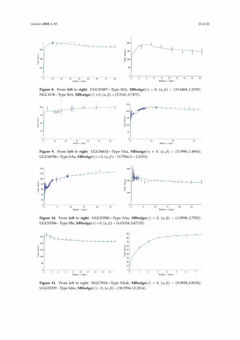
Figure 8. From left to right: UGC02487—Type S0A, SBbulge(r) ≠ 0, (α, β) = (19.4404, 1.2193).NGC4138 - Type S0A, SBbulge(r) ≠ 0, (α, β) = (5.5141, 0.7475).

Figure 9. From left to right: UGC06614—Type SAa, SBbulge(r) ≠ 0, (α, β) = (5.3990, 1.4964).UGC06786—Type SAa, SBbulge(r) ≠ 0, (α, β) = (9.7584, b = 2.0333).

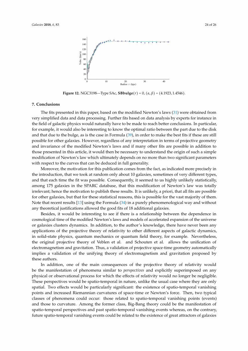
Figure 10. From left to right: UGC03580—Type SAa, SBbulge(r) ≠ 0, (α, β) = (1.8598, 3.7529).UGC03546 - Type SBa, SBbulge(r) ≠ 0, (α, β) = (6.03334, 0.67135).

Figure 11. From left to right: NGC7814—Type SAab, SBbulge(r) ≠ 0, (α, β) = (9.0958, 0.8154).UGC02259 - Type Sdm, SBbulge(r) = 0, (α, β) = (38.5594, 12.2014).

Galaxies 2018, 6, 83 24 of 26

Figure 12. NGC3198—Type SAc, SBbulge(r) = 0, (α, β) = (4.1923, 1.4546).

7. Conclusions

The fits presented in this paper, based on the modified Newton’s laws (31) were obtained fromvery simplified data and data processing. Further fits based on data analysis by experts for instance inthe field of galactic physics would naturally have to be made to reach better conclusions. In particular,for example, it would also be interesting to know the optimal ratio between the part due to the diskand that due to the bulge, as is the case in Formula (39), in order to make the best fits if these are stillpossible for other galaxies. However, regardless of any interpretation in terms of projective geometryand invariance of the modified Newton’s laws and if many other fits are possible in addition tothose presented in this article, it would then be necessary to understand the origin of such a simplemodification of Newton’s law which ultimately depends on no more than two significant parameterswith respect to the curves that can be deduced in full generality.

Moreover, the motivation for this publication comes from the fact, as indicated more precisely inthe introduction, that we took at random only about 10 galaxies, sometimes of very different types,and that each time the fit was possible. Consequently, it seemed to us highly unlikely statistically,among 175 galaxies in the SPARC database, that this modification of Newton’s law was totallyirrelevant; hence the motivation to publish these results. It is unlikely, a priori, that all fits are possiblefor other galaxies, but that for these statistical reasons, this is possible for the vast majority of them.Note that recent results [13] using the Formula (34) in a purely phenomenological way and withoutany theoretical justifications allowed the good fits of 18 additional galaxies.

Besides, it would be interesting to see if there is a relationship between the dependence incosmological time of the modified Newton’s laws and models of accelerated expansion of the universeor galaxies clusters dynamics. In addition, to the author’s knowledge, there have never been anyapplications of the projective theory of relativity to other different aspects of galactic dynamics,in solid-state physics, quantum mechanics or quantum field theory, for example. Nevertheless,the original projective theory of Veblen et al. and Schouten et al. allows the unification ofelectromagnetism and gravitation. Thus, a validation of projective space-time geometry automaticallyimplies a validation of the unifying theory of electromagnetism and gravitation proposed bythese authors.

In addition, one of the main consequences of the projective theory of relativity wouldbe the manifestation of phenomena similar to perspectives and explicitly superimposed on anyphysical or observational process for which the effects of relativity would no longer be negligible.These perspectives would be spatio-temporal in nature, unlike the usual case where they are onlyspatial. Two effects would be particularly significant: the existence of spatio-temporal vanishingpoints and increased Riemannian curvatures of space-time or Newton’s force. Then, two typicalclasses of phenomena could occur: those related to spatio-temporal vanishing points (events)and those to curvature. Among the former class, Big-Bang theory could be the manifestation ofspatio-temporal perspectives and past spatio-temporal vanishing events whereas, on the contrary,future spatio-temporal vanishing events could be related to the existence of great attractors of galaxies

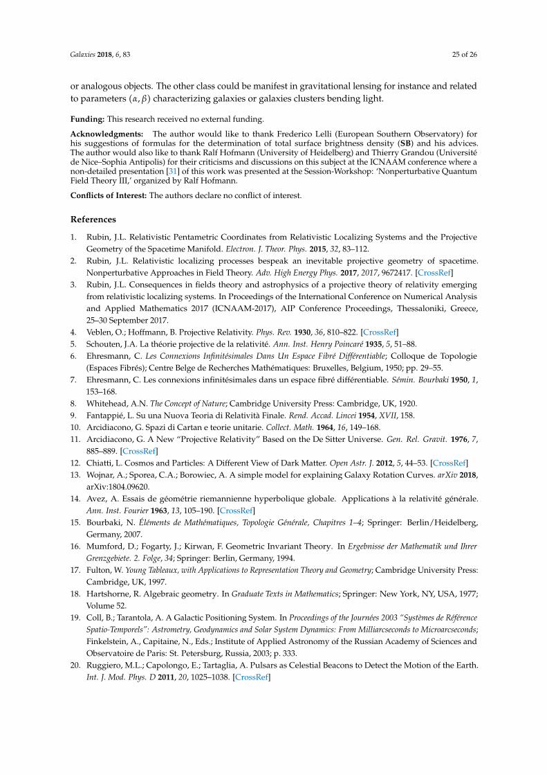
Galaxies 2018, 6, 83 25 of 26

or analogous objects. The other class could be manifest in gravitational lensing for instance and relatedto parameters (α, β) characterizing galaxies or galaxies clusters bending light.

Funding: This research received no external funding.

Acknowledgments: The author would like to thank Frederico Lelli (European Southern Observatory) forhis suggestions of formulas for the determination of total surface brightness density (SB) and his advices.The author would also like to thank Ralf Hofmann (University of Heidelberg) and Thierry Grandou (Universitéde Nice–Sophia Antipolis) for their criticisms and discussions on this subject at the ICNAAM conference where anon-detailed presentation [31] of this work was presented at the Session-Workshop: ‘Nonperturbative QuantumField Theory III,’ organized by Ralf Hofmann.

Conflicts of Interest: The authors declare no conflict of interest.

References

1. Rubin, J.L. Relativistic Pentametric Coordinates from Relativistic Localizing Systems and the ProjectiveGeometry of the Spacetime Manifold. Electron. J. Theor. Phys. 2015, 32, 83–112.

2. Rubin, J.L. Relativistic localizing processes bespeak an inevitable projective geometry of spacetime.Nonperturbative Approaches in Field Theory. Adv. High Energy Phys. 2017, 2017, 9672417. [CrossRef]

3. Rubin, J.L. Consequences in fields theory and astrophysics of a projective theory of relativity emergingfrom relativistic localizing systems. In Proceedings of the International Conference on Numerical Analysisand Applied Mathematics 2017 (ICNAAM-2017), AIP Conference Proceedings, Thessaloniki, Greece,25–30 September 2017.

4. Veblen, O.; Hoffmann, B. Projective Relativity. Phys. Rev. 1930, 36, 810–822. [CrossRef]5. Schouten, J.A. La théorie projective de la relativité. Ann. Inst. Henry Poincaré 1935, 5, 51–88.6. Ehresmann, C. Les Connexions Infinitésimales Dans Un Espace Fibré Différentiable; Colloque de Topologie

(Espaces Fibrés); Centre Belge de Recherches Mathématiques: Bruxelles, Belgium, 1950; pp. 29–55.7. Ehresmann, C. Les connexions infinitésimales dans un espace fibré différentiable. Sémin. Bourbaki 1950, 1,

153–168.8. Whitehead, A.N. The Concept of Nature; Cambridge University Press: Cambridge, UK, 1920.9. Fantappié, L. Su una Nuova Teoria di Relatività Finale. Rend. Accad. Lincei 1954, XVII, 158.10. Arcidiacono, G. Spazi di Cartan e teorie unitarie. Collect. Math. 1964, 16, 149–168.11. Arcidiacono, G. A New “Projective Relativity” Based on the De Sitter Universe. Gen. Rel. Gravit. 1976, 7,

885–889. [CrossRef]12. Chiatti, L. Cosmos and Particles: A Different View of Dark Matter. Open Astr. J. 2012, 5, 44–53. [CrossRef]13. Wojnar, A.; Sporea, C.A.; Borowiec, A. A simple model for explaining Galaxy Rotation Curves. arXiv 2018,

arXiv:1804.09620.14. Avez, A. Essais de géométrie riemannienne hyperbolique globale. Applications à la relativité générale.

Ann. Inst. Fourier 1963, 13, 105–190. [CrossRef]15. Bourbaki, N. Éléments de Mathématiques, Topologie Générale, Chapitres 1–4; Springer: Berlin/Heidelberg,

Germany, 2007.16. Mumford, D.; Fogarty, J.; Kirwan, F. Geometric Invariant Theory. In Ergebnisse der Mathematik und Ihrer

Grenzgebiete. 2. Folge, 34; Springer: Berlin, Germany, 1994.17. Fulton, W. Young Tableaux, with Applications to Representation Theory and Geometry; Cambridge University Press:

Cambridge, UK, 1997.18. Hartshorne, R. Algebraic geometry. In Graduate Texts in Mathematics; Springer: New York, NY, USA, 1977;

Volume 52.19. Coll, B.; Tarantola, A. A Galactic Positioning System. In Proceedings of the Journées 2003 “Systèmes de Référence

Spatio-Temporels”: Astrometry, Geodynamics and Solar System Dynamics: From Milliarcseconds to Microarcseconds;Finkelstein, A., Capitaine, N., Eds.; Institute of Applied Astronomy of the Russian Academy of Sciences andObservatoire de Paris: St. Petersburg, Russia, 2003; p. 333.

20. Ruggiero, M.L.; Capolongo, E.; Tartaglia, A. Pulsars as Celestial Beacons to Detect the Motion of the Earth.Int. J. Mod. Phys. D 2011, 20, 1025–1038. [CrossRef]

Galaxies 2018, 6, 83 26 of 26

21. Winternitz, L.B.; Hassouneh, M.A.; Mitchell, J.W.; Price, S.R.; Yu, W.H.; Semper, S.R.; Ray, P.S.; Wood, K.S.;Arzoumanian, Z.; Gendreau, K.C. SEXTANT X-ray Pulsar Navigation Demonstration: Additional On-OrbitResults. In Proceedings of the 2018 SpaceOps Conference, SpaceOps Conferences, (AIAA 2018-2538), Marseille,France, 28 May 2018. [CrossRef]

22. Hawking, S.W.; Ellis, G.F.R. The Large Scale Structure of Space–time. In Cambridge Monographs on MathematicalPhysics; Cambridge University Press: New York, NY, USA, 1973.

23. Penrose, R. Gravitational collapse and spacetime singularities. Phys. Rev. Lett. 1965, 14, 57–59. [CrossRef]24. Hawking, S.W.; Penrose, R. The singularities of Gravitational Collapse and Cosmology. Proc. Roy. Soc. Lond. A

1970, 314, 529–548. [CrossRef]25. Kluwick, A. Shock discontinuities: from classical to non-classical shocks. Acta Mech. 2018, 229, 515–533.

[CrossRef]26. Hawking, S.W. Information Preservation and Weather Forecasting for Black Holes. arXiv 2014,

arXiv:1401.5761.27. Famaey, B.; McGaugh, S.S. Modified Newtonian Dynamics (MOND): Observational Phenomenology and

Relativistic Extensions. Living Rev. Relativ. 2012, 15, 10. [CrossRef] [PubMed]28. SPARC Database Is Maintained by Federico Lelli. Available online: http://astroweb.cwru.edu/SPARC/

(accessed on 17 July 2017).29. Lelli, F.; McGaugh, S.S.; Schombert, J.M. SPARC: Mass Models for 175 Disk Galaxies with Spitzer Photometry

and Accurate Rotation Curves. Astro. J. 2016, 152, 157. [CrossRef]30. Schombert, J. ARCHANGEL: Galaxy Photometry System. Astrophysics Source Code Library, ASCL Record:

1107.011, July 2011. Available online: http://abyss.uoregon.edu/∼js/archangel/ (accessed on 1 January 2018).31. Rubin, J.L. Rotational Velocity Fields of Galaxies and Projective Geometry of Spacetime. 2017. Available

online: https://hal.inria.fr/hal-01637022 (accessed on 3 August 2018).

© 2018 by the author. Licensee MDPI, Basel, Switzerland. This article is an open accessarticle distributed under the terms and conditions of the Creative Commons Attribution(CC BY) license (http://creativecommons.org/licenses/by/4.0/).