projection-based curve clustering
TRANSCRIPT

Projection-based curve clustering
Benjamin AUDER
DEN/DER/SESI/LCFR
CEA Cadarache
13108 SAINT PAUL LEZ DURANCE Cedex, FRANCE
Aurélie FISCHER∗
Laboratoire de Statistique Théorique et Appliquée
Université Pierre et Marie Curie – Paris VI
Boîte 158, couloir 15–16, 2e étage
4 place Jussieu, 75252 PARIS Cedex 05, FRANCE
Abstract – This paper focuses on unsupervised curve classification in the contextof nuclear industry. At the Commissariat à l’Energie Atomique (CEA), Cadarache(France), the thermal-hydraulic computer code CATHARE is used to study the re-liability of reactor vessels. The code inputs are physical parameters and the outputsare time evolution curves of a few other physical quantities. As the CATHARE codeis quite complex and CPU-time consuming, it has to be approximated by a regres-sion model. This regression process involves a clustering step. In the present paper,CATHARE output curves are clustered using a k-means scheme, with a projectiononto a lower dimensional space. We study the properties of the empirically optimalcluster centers found by the clustering method based on projections, compared tothe “true” ones. The choice of the projection basis is discussed, and an algorithmis implemented to select the best projection basis among a library of orthonormalbases. The approach is illustrated on a simulated example and then applied to theindustrial problem.
Index Terms — Clustering, basis expansion, projections, k-means, wavelet packets.
∗Corresponding author. E-mail: [email protected]
1

1 Introduction
1.1 The CATHARE code
A major concern in nuclear industry is the life span of reactor vessels. To go onusing the current nuclear reactors, their reliability has to be proved. For this pur-pose, complex computer codes are developed to simulate the behavior of the vesselunder different sequences of accidents. At the Commissariat à l’Energie Atomique(CEA), Cadarache (France), one of the main types of accident under study is thepressurized thermal shock. This is a problem due to the combined stresses from arapid temperature and pressure change. More specifically, as a reactor vessel getsolder, the potential for failure by cracking when it is cooled rapidly at high pressureincreases greatly. The analysis of pressurized thermal shock is made of two mainsteps. First, a thermal-hydraulic analysis is done to determine the temporal evolu-tions of temperature, pressure and thermal exchange coefficient in the vessel annularspace, since these features have an influence on the mechanical and thermal chargeon the vessel inner surface. Some evolution curves x1(t), . . . , xn(t) corresponding tothe thermal exchange coefficient are depicted in Figure 1 (n = 66). Each curve xi(t)is obtained as the simulation result for a certain vector of input physical parameters.The curves of temperature, pressure and thermal exchange coefficient obtained dur-ing this first step are then used as limit conditions in the second part of the analysis,which is a mechanical investigation aiming at checking if some defects on the ves-sel annular space could propagate and gain importance to such an extent that thiswould cause a break of the vessel inner surface. For further details on the reliabilityof reactor vessels, we refer the reader to Auder, De Crecy, Iooss, and Marquès [5].
The simulation step relies on a computer code called CATHARE (Code Avancé deTHermohydraulique pour les Accidents des Réacteurs à Eau, in English Code forAnalysis of THermalhylaudrics during an Accident of Reactor and safety Evalua-tion). The CATHARE code is a system code for pressurized water reactors safetyanalysis, accident management, definition of plant operating procedures and forresearch and development. The project is a result of a joint effort of the reac-tor vendor AREVA, the CEA, EDF (Electricité de France) and the IRSN (Institutde Radioprotection et de Sûreté Nucléaire). The first delivered version V1.3L wasavailable in 1997. The CEA team CATHARE located in Grenoble (France) is incharge of the development, the assessment and the maintenance of the code. (Seehttp://www-cathare.cea.fr.)
The CATHARE code allows to simulate the evolution of temperature, pressure andthermal exchange coefficient, given the physical parameters as inputs. However, thiscode is so slow (about 6 to 10 hours for one run) that it cannot be used directlyfor reliability calculations. To bypass this obstacle, the strategy drawn up by theCEA is to build a so-called metamodel which is a fast approximation of the originalcode, precise enough to carry out statistical computations. The term “metamodel”indicates that a computer code approximating a physical process has already beendeveloped, and now this code is modeled in turn. Here, the purpose is the con-struction of a regression model based on a few hundreds CATHARE code outputs,
2

Figure 1: 66 evolution curves of thermal exchange coefficient in a nuclear vessel.
Input physical parametersϕ1, . . . , ϕn ∈ R
p
(pumps rotation speed,fluid velocities, batteryliquid volume, massfraction of nitrogenin battery liquid. . . )
Output curvesx1(t), . . . , xn(t)
CATHARE
Computer code
Metamodel
Clustering + RegressionNew inputϕ ∈ R
pPredicted curve
x(t)
Figure 2: Flowchart of the CATHARE code.
3

obtained during one week of computation on a supercomputer in 2007. The inputswere sampled randomly by latin hypercube methods (see, e.g., McKay, Conover,and Beckman [28] and Loh [26]), so that we have no control over the inputs inthe learning sample. As different kinds of behavior for temperature, pressure andthermal exchange coefficient may be observed depending on the physical parame-ters, a preliminary unsupervised classification of CATHARE code output curves isessential. Once the curves have been clustered in meaningful classes, the regressionmodel can be adjusted for each group of outputs separately. The clustering step isthe object of the present paper.
1.2 Clustering
Clustering is the problem of partitioning data into a finite number of groups (de-noted hereafter by k), or clusters, so that the data items inside each of them arevery similar among themselves and as different as possible from the elements of theother clusters (Duda, Hart, and Stork [14, Chapter 10]). In our industrial context,the data is made of evolution curves of temperature, pressure or thermal exchangecoefficient. Using a probabilistic point of view, these curves can be seen as indepen-dent draws X1(t), . . . , Xn(t) with the same distribution as a generic random variableX(t) taking values in a functional space (E, ‖ · ‖) — typically, the Hilbert space ofsquare integrable functions.
A widely used clustering method is the so-called k-means clustering, which consistsin partitioning the random observations X1, . . . , Xn ∈ E into k classes by minimizingthe empirical distortion
W∞,n(c) =1
n
n∑
i=1
min`=1,...,k
‖Xi − c`‖2,
over all possible cluster centers c = (c1, . . . , ck) ∈ Ek. Here, µn denotes the empiricalmeasure associated with the sample X1, . . . , Xn, i.e.,
µn(A) =1
n
n∑
i=1
1{Xi∈A}
for every Borel subset A of E. In other words, we look for a Voronoi partition of E.The Voronoi partition C1, . . . , Ck associated with c = (c1, . . . , ck) ∈ Ek is defined byletting an element x ∈ E belong to C` if it is closer (with respect to the norm ‖ · ‖)to c` than to any other cj (ties are broken arbitrarily). The `-th cluster is made ofthe observations Xi assigned to c`, or equivalently, falling in the Voronoi cell C`. Inthis framework, the accuracy of the clustering scheme is assessed by the distortionor mean squared error
W∞(c) = E
[
min`=1,...,k
‖X − c`‖2]
,
where E stands for expectation with respect to the distribution of X. This clusteringmethod is in line with the more general theory of quantization. More specifically, it
4

corresponds to the empirical version of nearest neighbor quantization (Linder [24],Gersho and Gray [18], Graf and Luschgy [21]). However, the problem of finding aminimizer of the criterion W∞,n(c) is in general NP-hard, and there is no efficientalgorithm to find the optimal solution in reasonable time. That is why severaliterative algorithms have been developed to give approximate solutions. One of thefirst to be described historically is Lloyd’s algorithm (Lloyd [25]).
The challenge is to adapt the k-means clustering method to our setting. The maindifficulty here is the high dimensionality of the data, which casts the problem intothe general class of functional statistics. For a comprehensive introduction to thistopic, see Ramsay and Silverman [32] and Ferraty and Vieu [15]. A possible approachto reduce the infinite dimension of the observations X1, . . . , Xn consists in project-ing them onto a lower-dimensional subspace. In this context, Abraham, Cornillon,Matzner-Løber, and Molinari [1] project the curves on a B-spline basis, and get clus-ters with the k-means algorithm applied to the coefficients. These authors argue thatprojecting onto a smooth spline basis plays the role of a denoising procedure, giventhat the observed curves could contain measurement errors, and also allows to dealwith curves which were not measured at the same time. James and Sugar [23] use aB-spline basis to model the centers of the clusters and write each curve in cluster ` asa main effect defined by spline coefficients plus an error term. This allows for somedeviations around a model curve specific to cluster `. The authors add a Gaussianerror term to model the individual variations among one cluster. This way, the maineffect is enriched, and the model can take into account more complex behaviors. Themethod in Gaffney [17] is similar, also with a B-spline basis. Another option is touse a Self-Organizing Map algorithm on the coefficients (Rossi, Conan-Guez, and ElGolli [33]), again obtained by projecting the functions onto a B-spline basis. Thesebases are often used because they are easy to implement, and require a relativelyminimal number of parametric assumptions. Besides, Biau, Devroye, and Lugosi [6]examine the theoretical performance of clustering with random projections basedon the Johnson-Lindenstrauss Lemma, which represent a sound alternative to or-thonormal projections thanks to their distance-preserving properties. Chiou and Li[7] propose a method which generalizes the k-means algorithm to some extent, byconsidering covariance structures via functional principal component analysis. Inthe approach of these authors, each curve is decomposed on an adaptive local basis(valid for the elements in the cluster), and the clusters are determined according tothe full approximation onto each basis. In the wavelet-based method for functionaldata clustering developed in Antoniadis, Brossat, Cugliari, and Poggi [3], a smoothcurve is reduced to a finite number of representative features, by considering thecontribution of each wavelet coefficient to the global energy of the curve.
In the present contribution, we propose to investigate the problem of clusteringoutput curves X1, . . . , Xn of the CATHARE code, assuming that they arise from arandom variable X taking its values in some subset of the space of square integrablefunctions. As a general strategy, we reduce the infinite dimension ofX by consideringonly the first d coefficients of the expansion on a Hilbertian basis, and then performclustering in R
d. We study the theoretical properties of this clustering method withprojection. A bound expressing what is lost when replacing the empirically optimal
5

cluster centers by the centers obtained by projection is offered (Section 2). Sincethe result may depend on the basis choice, several projection bases are used inpractice, and we look for the best one minimizing a given criterion. To this end, analgorithm based on Coifman and Wickerhauser [9] is implemented, searching for anoptimal basis among a library of wavelet packet bases available in the R packagewmtsa, and this “optimal basis” is compared with the Fourier basis, the Haar basis,and the functional principal component basis (Section 3). Finally, this algorithm isapplied to a simulated example and to our industrial problem (Section 4). Proofsare postponed to Section 5.
2 Finite-dimensional projection for clustering
As mentioned earlier, we are concerned with square integrable functions. Since allresults can be adapted to L2([a, b]) by an appropriate rescaling, we consider for thesake of simplicity the space L2([0, 1]). As an infinite-dimensional separable Hilbertspace, L2([0, 1]) is isomorphic via the choice of a Hilbertian basis to the space `2 ofsquare-summable sequences. We focus more particularly on functions in L2([0, 1])whose coefficients in the expansion on a given Hilbertian basis belong to the subsetS of `2 given by
S ={
x = (xj)j≥1 ∈ `2 :+∞∑
j=1
ϕjx2j ≤ R2
}
, (1)
where R > 0 and (ϕj)j≥1 is a nonnegative increasing sequence such that
limj→+∞
ϕj = +∞.
It is worth pointing out that S is closely linked with the basis choice, even if thebasis does not appear explicitly in the definition. To illustrate this important fact,three examples are discussed below.
Example 2.1 (Sobolev ellipsoids). For β ∈ N∗ and L > 0, the periodic
Sobolev class W per(β, L) is the space of all functions f ∈ [0, 1]→ R such that f (β−1)
is absolutely continuous,∫ 1
0 (f (β)(t))2dt ≤ L2 and f (`)(0) = f (`)(1) for ` = 0, . . . , β−1. Let (ψj)j≥1 denote the trigonometric basis. Then a function f =
∑+∞j=1 xjψj is in
W per(β, L) if and only if the sequence x = (xj)j≥1 of its Fourier coefficients belongsto
S =
{
x ∈ `2 :+∞∑
j=1
ϕjx2j ≤ R2
}
,
where
ϕj =
{
j2β for even j(j − 1)2β for odd j
and R =L
πβ.
For the proof of this result and further details about Sobolev classes, we refer thereader to the book of Tsybakov [36]. Note that the set S could also be defined byϕj = jreαj with α > 0 and r ≥ −α (Tsybakov [35]).
6

Example 2.2 (Reproducing Kernel Hilbert Spaces). Let K : [0, 1] ×[0, 1] → R be a Mercer kernel, i.e., K is continuous, symmetric and positive def-inite. Recall that a kernel K is said to be positive definite if for all finite sets{x1, . . . , xm}, the matrix A defined by aij = K(xi, xj) for 1 ≤ i, j ≤ m is positive
definite. For example, the Gaussian kernel K(x, y) = exp(− (x−y)2
σ2 ) and the kernelK(x, y) = (c2 + (x − y)2)−a with a > 0 are Mercer kernels. For x ∈ [0, 1], letKx : y 7→ K(x, y). Then, Moore-Aronszajn’s Theorem (Aronszajn [4]) states thatthere exists a unique Hilbert space (HK , 〈·, ·〉) of functions on [0, 1] such that:
1. For all x ∈ [0, 1], Kx ∈ HK .
2. The span of the set {Kx, x ∈ [0, 1]} is dense in HK.
3. For all f ∈ HK and x ∈ [0, 1], f(x) = 〈Kx, f〉.The Hilbert space HK is said to be the reproducing kernel Hilbert space (for short,RKHS) associated with the kernel K. Next, the operator K defined by
Kf : y 7→∫ 1
0K(x, y)f(x)dx
is self-adjoint, positive and compact. Consequently, there exists a complete orthonor-mal system (ψj)j≥1 of L2([0, 1]) such that Kψj = λjψj , where the set of eigenvalues{λj, j ≥ 1} is either finite or a sequence tending to 0 at infinity. Moreover, theλj are nonnegative. Suppose that K is not of finite rank — so that {λj, j ≥ 1} isinfinite — and that the eigenvalues are sorted in decreasing order, that is λj ≥ λj+1for all j ≥ 1. Clearly, there is no loss of generality in assuming that λj > 0 forall j ≥ 1. Indeed, if not, L2([0, 1]) is replaced by the linear subspace spanned by theeigenvectors corresponding to non-zero eigenvalues.
According to Mercer’s theorem, K has the representation
K(x, y) =+∞∑
j=1
λjψj(x)ψj(y),
where the convergence is absolute and uniform (Cucker and Smale [10, Chapter III,Theorem 1]). Moreover, HK may be characterized through the eigenvalues of theoperator K by
HK ={
f ∈ L2([0, 1]) : f =+∞∑
j=1
xjψj ,+∞∑
j=1
x2j
λj<∞
}
,
with the inner product
⟨ +∞∑
j=1
xjψj ,+∞∑
j=1
yjψj
⟩
=+∞∑
j=1
xjyjλj
(Cucker and Smale [10, Chapter III, Theorem 4]). Then, letting
S ={
x ∈ `2,+∞∑
j=1
x2j
λj≤ R2
}
,
the set S is of the desired form (1), with ϕj = 1/λj.
7

Example 2.3 (Besov ellipsoids and wavelets). Let α > 0. For f ∈ L2([0, 1]),the Besov semi-norm |f |Bα
2(L2) is defined by
|f |Bα2(L2) =
( +∞∑
j=0
[2jαωr(f, 2−j , [0, 1])2]
2)1/2
where ωr(f, t, [0, 1])2 denotes the modulus of smoothness of f, as defined for instancein DeVore and Lorentz [12], and r = bαc+ 1. Let Λ(j) be an index set at resolutionlevel j and (xj,`)j≥0,`∈Λ(j) the coefficients of the expansion of f in a suitable waveletbasis. Then, for f such that |f |Bα
2(L2) ≤ ρ, the coefficients xj,` satisfy
+∞∑
j=0
∑
`∈Λ(j)
22jαx2j,` ≤ ρ2C2,
where C > 0 depends only on the basis. We refer to Donoho and Johnstone [13] formore details.
Let us now come back to the general setting
S ={
x = (xj)j≥1 ∈ `2 :+∞∑
j=1
ϕjx2j ≤ R2
}
,
and consider the problem of clustering the sample X1, . . . , Xn with values in S. Somenotation and assumptions are in order. First, we will suppose that P {‖X‖ ≤ R} =1. Notice that the fact that X takes its values in S is in general not enough to implyP {‖X‖ ≤ R} = 1. Secondly, let j0 be the smallest integer j such that ϕj > 0. Toavoid technical difficulties, we require in the sequel d ≥ j0. For all d ≥ 1, we willdenote by Πd the orthogonal projection on R
d and let Sd = Πd(S). Lastly, observethat Sd identifies with the ellipsoid
{
x = (x1, . . . , xd) ∈ Rd :
d∑
j=1
ϕjx2j ≤ R2
}
.
As explained in the introduction, the criterion to minimize is
W∞,n(c) =1
n
n∑
i=1
min`=1,...,k
‖Xi − c`‖2,
and the performance of the clustering obtained with the centers c = (c1, . . . , ck) ∈ Skis measured by the distortion
W∞(c) = E
[
min`=1,...,k
‖X − c`‖2]
.
The quantityW ∗∞ = inf
c∈SkW∞(c)
8

represents the optimal risk we can achieve. With the intention of performing cluster-ing in the projection space Sd, we also introduce the “finite-dimensional” distortion
Wd(c) = E
[
min`=1,...,k
‖Πd(X)− Πd(c`)‖2]
and its empirical counterpart
Wd,n(c) =1
n
n∑
i=1
min`=1,...,k
‖Πd(Xi)− Πd(c`)‖2,
as well asW ∗d = inf
c∈SkWd(c).
Let us observe that, as the support of the empirical measure µn contains at most npoints, there exists an element cd,n which is a minimizer of Wd,n(c) on Sk. Moreover,in view of its definition, Wd,n(c) only depends on the centers projection Πd(c) (onehas Wd,n(c) = Wd,n(Πd(c)) for all c) and we can thus assume that cd,n ∈ (Sd)k.Notice also that for all c ∈ S,
‖Πd(X)− Πd(c)‖2 ≤ ‖X − c‖2
(the projection Πd is 1-Lipschitz), which implies that
Wd(c) ≤ W∞(c)
for all c.
The following lemma provides an upper bound for the maximal deviation
supc∈Sk
[W∞(c)−Wd(c)].
Lemma 2.1. We have
supc∈Sk
[W∞(c)−Wd(c)] ≤ 4R2
ϕd.
We are now in a position to state the main result of this section.
Theorem 2.1. Let cd,n ∈ (Sd)k be a minimizer of Wd,n(c). Then,
E[W∞(cd,n)]−W ∗∞ ≤ E[Wd(cd,n)]−W ∗d +8R2
ϕd. (2)
Theorem 2.1 expresses the fact that the expected excess clustering risk in the infinitedimensional space is bounded by the corresponding “finite-dimensional risk” plus anadditional term representing the price to pay when projecting onto Sd. Yet, the firstterm in the right-hand side of inequality (2) above is known to tend to 0 when ngoes to infinity. More precisely, as P {‖Πd(X)‖ ≤ R} = 1, we have
E[Wd(cd,n)]−W ∗d ≤Ck√n,
9
where C = 12R2 (Biau, Devroye, and Lugosi [6]). In our setting, to keep the samerate of convergence O(1/
√n) in spite of the extra term 8R2/ϕd, ϕd must be of
the order√n. For Sobolev ellipsoids (Example 2.1), where ϕj ≥ (j − 1)2β, this
means a dimension d of the order n1/4β . When ϕj = jreαj , the rate of convergenceis O(1/
√n) as long as d is chosen of the order lnn/(2α). In the RKHS context
(Example 2.2), consider the case of eigenvalues {λj, j ≥ 1} with polynomial orexponential-polynomial decay, which covers a broad range of kernels (Williamson,Smola, and Schölkopf [38]). If λj = O(j−(α+1)), α > 0, then 1/ϕd = O(d−(α+1)),and d must be of the order n1/(2α+2), whereas λj = O(e−αj
p
), α, p > 0, leads to aprojection dimension d of the order (lnn/(2α))1/p. Obviously, the upper bound (2)is better for large ϕd, and consequently large d. Nevertheless, from a computationalpoint of view, the projection dimension should not be chosen too large.
Remark 2.1. Throughout, we assumed that P {‖X‖ ≤ R} = 1. This requirement,called the peak power constraint, is standard in the clustering and signal processingliterature. We do not consider in this paper the case where this assumption is notsatisfied, which is feasible but leads to technical complications (see Merhav andZiv [29], Biau, Devroye, and Lugosi [6] for results in this direction). Besides, thenumber of clusters is assumed to be fixed throughout the paper. Several methodsfor estimating k have been proposed in the literature (see, e.g., Milligan and Cooper[31] and Gordon [20]).
As already mentioned, the subset of coefficients S is intimately connected to theunderlining Hilbertian basis. As a consequence, all the results presented stronglydepend on the orthonormal system considered. Therefore, the choice of a properbasis is crucial and is discussed in the next section.
3 Basis selection
Wavelet packet best basis algorithm In this section, we describe an algorithmsearching for the best projection basis among a “library”. If {ψα, α ∈ I} ⊂ L2([0, 1])is a collection of elements in L2([0, 1]) which span L2([0, 1]) and allow to build severaldifferent bases by choosing various subsets {ψα, α ∈ Iβ} ⊂ L2([0, 1]), the collectionof bases built this way is called a library of bases. Here, I is some index set, and βruns over some other index set.
More specifically, we focus on the best basis algorithm of Coifman and Wickerhauser[9] (see also Wickerhauser [37]), which yields an optimal basis among a library ofwavelet packets. Wavelets are functions which cut up a signal into different fre-quency components to study each component with a resolution matched to its scale.Unlike the Fourier basis, wavelets are localized both in time and frequency. Hence,they have advantages over traditional Fourier methods when the signal contains dis-continuities as well as noise. For detailed expositions of the mathematical aspectsof wavelets, see the books of Daubechies [11], Mallat [27] and Meyer [30].
10

Let the sequence of functions (ψν)ν≥0 be defined by
ψ0(t) = Hψ0(t),∫
R
ψ0(t)dt = 1,
ψ2ν(t) = Hψν(t) =√
2∑
p∈Z
h(p)ψν(2t− p),
ψ2ν+1(t) = Gψν(t) =√
2∑
p∈Z
g(p)ψν(2t− p),
where H and G are orthogonal quadrature filters, i.e., convolution-decimation op-erators satisfying some algebraic properties (see, e.g., Wickerhauser [37]). Let Λνdenote the closed linear span of the translates ψν(· − p), p ∈ Z, of ψν , and
σsΛν = {2−s/2x(2−st), x ∈ Λν}.
To every such subspace of L2(R) corresponds a dyadic interval
Isν =[
ν
2s,ν + 1
2s
[
.
For all (s, ν), these subspaces give an orthogonal decomposition
σsΛν = σs+1Λ2ν � σs+1Λ2ν+1.
Observe that for ν = 0, . . . , 2s − 1, the Isν are dyadic subintervals of [0, 1[ .
The next proposition provides a library of orthonormal bases built with functions ofthe form ψsνp = 2−s/2ψν(2
−st−p), called wavelet packets of scale index s, frequencyindex ν and position index p.
Proposition 3.1 (Wickerhauser [37]). If s ≤ L for some finite maximum L, H andG are orthogonal quadrature filters and I is a collection of disjoint dyadic intervalswhose union is R
+, then BI = {ψsνp, p ∈ Z, Isν ∈ I} is an orthonormal basis forL2(R). Moreover, if I is a disjoint dyadic cover of [0, 1[, then BI is an orthonormalbasis of Λ0.
This construction yields orthonormal bases of L2(R). Some changes must be madeto obtain bases of L2([0, 1]). Roughly, they consist in considering not all scalesand shifts, and adapting the wavelets which overlap the boundary of [0, 1] (see forinstance Cohen, Daubechies, and Vial [8]).
The library can be seen as a binary tree whose nodes are the spaces σsΛν (Figure 3and 4). An orthonormal basis is given by the leaves of some subtree. Figure 5 and6 show two examples of bases which can be obtained in this way.
To define an optimal basis, a notion of information cost is needed. Coifman andWickerhauser [9] propose to use Shannon entropy. In our context, the basis choicewill be done with respect to some reference curve x0 which has to be representativeof the data. We compute, for each basis in the library, the Shannon entropy of thecoefficients of x0 in this basis, and select the basis minimizing this entropy. The
11

Λ0
σ1Λ0 σ1Λ1
σ2Λ0 σ2Λ1 σ2Λ2 σ2Λ3
σ3Λ0 σ3Λ1 σ3Λ2 σ3Λ3 σ3Λ4 σ3Λ5 σ3Λ6 σ3Λ7
Figure 3: Tree structure of wavelet packet bases.
[0, 1[
[0, 12[ [ 1
2, 1[
[0, 14[ [ 1
4, 1
2[ [ 1
2, 3
4[ [ 3
4, 1[
[0, 18[ [ 1
8, 1
4[ [ 1
4, 3
8[ [ 3
8, 1
2[ [ 1
2, 5
8[ [ 5
8, 3
4[ [ 3
4, 7
8[ [ 7
8, 1[
Figure 4: Correspondence with dyadic covers of [0,1[ .
12

Λ0
σ1Λ0 σ1Λ1
σ2Λ0 σ2Λ1 σ2Λ2 σ2Λ3
σ3Λ0 σ3Λ1 σ3Λ2 σ3Λ3 σ3Λ4 σ3Λ5 σ3Λ6 σ3Λ7
Figure 5: The wavelet basis.
Λ0
σ1Λ0 σ1Λ1
σ2Λ0 σ2Λ1 σ2Λ2 σ2Λ3
σ3Λ0 σ3Λ1 σ3Λ2 σ3Λ3 σ3Λ4 σ3Λ5 σ3Λ6 σ3Λ7
Figure 6: An example of fixed level wavelet packet basis.
13

construction of this best basis, relying on the binary tree structure of the library, isachieved by comparing, at each node, starting from the bottom of the tree, parentswith their two children. We decided to take for x0 the median curve in the samplein the L2 norm sense. Indeed, it is more likely to present characteristic behaviorsof the other curves than the mean, because the mean curve is a smooth averagerepresentative, which is probably too easy to approximate with a few basis functions.However, we observed that these two functions surprisingly give rise to almost thesame basis. Both choices are thus possible. The mean curve is useful if we knowthat some noise has to be removed, whereas the median curve seems a better choiceto reflect the small-scale irregularities.
We have implemented the algorithm in R, and it has been run through all filtersavailable in the R package wmtsa. These filters belong to four families, extremalphase family (Daubechies wavelets), including Haar basis, least asymmetric family(Symmlets), “best localized” wavelets and Coiflets. For example, the least asym-metric family contains ten different filters “s2”, “s4”, “s6”, “s8”, “s10”, “s12”, “s14”,“s16”, “s18”, “s20”. Finally, we keep the clustering result obtained with the basisminimizing the distortion among the various filters. In the sequel, this basis will becalled Best-Entropy basis.
In the applications, the performance of the Best-Entropy basis will be compared withthe Haar wavelet basis, the Fourier basis and the functional principal componentanalysis basis. For the sake of completeness, we recall here the definition of thesebases.
The Haar wavelet basis Let φ(t) = 1[0,1](t) and ψ(t) = 1[0,1/2[(t) − 1[1/2,1](t).Then, the family {φ, ψj,`}, where
ψj,`(t) = 2j/2ψ(2jt− `), j ≥ 0, 0 ≤ ` ≤ 2j − 1,
constitutes a Hilbertian basis of L2([0, 1]), called Haar basis.
Figure 7: Haar scaling function φ and mother wavelet function ψ.
14

The Fourier basis The Fourier basis on [0, 1] is the complete orthonormal systemof L2([0, 1]) built with the trigonometric functions
ψ1(t) = 1, ψ2j(t) =√
2 cos(2πjt), ψ2j+1(t) =√
2 sin(2πjt), j ≥ 1.
Functional principal component analysis Principal component analysis for func-tional data (for short, functional PCA) is the generalization of the usual principalcomponent analysis for vector data. The Euclidean inner product is replaced by theinner product in L2([0, 1]). More precisely, functional PCA consists in writing Xi(t)under the form
Xi(t) = EX(t) ++∞∑
j=1
xijψj(t),
where the (xij)j≥1 and the functions (ψj)j≥1 are defined as follows. At the first step,the function ψ1 is chosen to maximize
1
n
n∑
i=1
x2i1 =
1
n
n∑
i=1
[
∫
ψ1(t)Xi(t)dt
]2
subject to∫
ψ1(t)2dt = 1.
Then, each ψj is computed by maximizing
1
n
n∑
i=1
x2ij
subject to∫
ψj(t)2dt = 1
and to the orthogonality constraints∫
ψ`(t)ψj(t)dt = 0, 1 ≤ ` ≤ j − 1.
Functional PCA can be characterized in terms of the eigenanalysis of covarianceoperators. If (λj)j≥1 denotes the eigenvalues and (ψj)j≥1 the eigenfunctions of theoperator C defined by C(f)(s) =
∫ 10 C(s, t)f(t)dt, where C(s, t) = cov(X(s), X(t)),
then
Xi(t) = EX(t) ++∞∑
j=1
xijψj(t),
where the xj are uncorrelated centered random variables with variance E[x2ij ] = λj .
There are similarities with the context of Example 2.2, but here the kernel dependson X. In practice, the decomposition can easily be computed with discrete matrixoperations, replacing C(s, t) by the covariance matrix of the Xi. This basis has somenice properties. In particular, considering a fixed number of coefficients, it minimizesamong all orthogonal bases the average squared L2 distance between the originalcurve and its linear representation (see, e.g., the book of Ghanem and Spanos [19]).
15

For more details on functional PCA, we refer the reader to Ramsay and Silverman[32].
Observe that since the functional PCA basis is a stochastic basis and the Best-Entropy basis algorithm also uses the data, rigorously the sample should be dividedinto two subsamples, one to build the basis, and the other for clustering.
4 Experimental results and analysis
We evaluated the performance of the clustering method with projection, using thevarious bases described in the previous section, for two different kinds of curves.First, a simulated example where the right clusters are known is discussed, to illus-trate the efficiency of the method. Then, we focus on our industrial problem andcluster output curves of a “black box” computer code.
Observe that, although the curves considered in Section 2 and Section 3 were truefunctions, in practice, we have to deal with curves sampled on a finite number ofdiscretization points. Therefore, a preprocessing step based on spline interpolationis necessary.
4.1 Synthetic control chart time series
Control chart time series are used for monitoring process environments, to achieveappropriate control and to produce high quality products. Different types of seriescan be encountered, but only one, a kind of white noise, indicates a normal working.All the other types of series must be detected, because they correspond to abnormalbehavior of the process.
The data set contains a few hundreds to a few thousands curves generated by theprocess described in Alcock and Manolopoulos [2], discretized on 128 time points.There are six types of curves: normal, cyclic, increasing trend, decreasing trend,upward shift and downward shift, which are represented in Figure 8. The equationswhich generated the data are indicated below.
(A) Normal pattern: y(t) = m+ rs where m = 30, s = 2 and r ∼ U(−3, 3).
(B) Cyclic pattern: y(t) = m+ rs+ a sin 2πtT
where a, T ∼ U(10, 15).
(C) Increasing shift: y(t) = m+ rs+ gt with g ∼ U(0.2, 0.5).
(D) Decreasing shift: y(t) = m+ rs− gt.
(E) Upward shift: y(t) = m + rs + hx where x ∼ U(7.5, 20), h = 1[t0,D], t0 ∼U(
D3, 2D
3
)
, and D is the number of discretization points.
(F) Downward shift: y(t) = m+ rs− hx.
16

Figure 8: 10 example curves for each of the 6 types of control chart.
The two main advantages using this synthetic data set is that we can simulate asmany curves as we wish and we know the right clusters.
The k-means algorithm on the projected coefficients has been run for all four bases(Best-Entropy, Haar, functional PCA and Fourier basis), with varying sample size nand projection dimension d. Since the result of a k-means algorithm may depend onthe choice of the initial centers, the algorithm is restarted 100 times. The maximumnumber of iterations per run is set to 500. This program tries to globally minimizethe projected empirical distortion Wd,n(c). To evaluate its performance, we computean approximation W (d, n) of the distortion W∞(cd,n) using a set of 18000 samplecurves. This is possible in this simulated example, since we can generate as manycurves as we want. The distortion W (d, n) is computed for d varying from 2 to 50and n ranging from 100 to 3100. We restricted ourselves to the case d ≤ 50, sincethere are only 128 discretization points. Moreover, as pointed out earlier, d must notbe too large for computational complexity reasons. Indeed, a projection dimensiond = 50 is already high for a practical use.
Figures 9 and 10 show the contours plots corresponding to the evolution of W (d, n)as a function of d and n, for the functional PCA and the Haar basis. We remark thatthe norm of the gradient of W (d, n) vanishes when d and n are close to their maximalvalues. Hence, as expected according to Theorem 2.1, W (d, n) is decreasing in d andn. When d or n is too small (for instance d = 2 or n = 100), the clustering resultsare inaccurate. Besides, they are not stable with respect to the n observationschosen. However, for larger values of these parameters, the partitions obtainedquickly become satisfactory. The choice n ≥ 300 together with d ≥ 6 generally
17

Figure 9: Contour plot of W (d, n) for the functional PCA basis.
Figure 10: Contour plot of W (d, n) for the Haar basis.
18
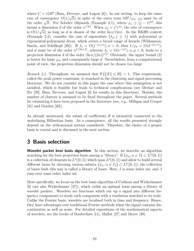
provides good results and is reasonably low for many applications.
Figure 11 shows the curve corresponding to the evolution of W (d, n) as a functionof d for n = 500, for all four bases, whereas Figure 12 represents the evolution ofW (d, n) versus n for d = 10. According to Section 2, ϕd must be of the order
√n.
For n = 500,√n is about 22. Considering that ϕd and d are approximately of the
same order, a projection dimension close to 22 should thus be suitable. Indeed, wesee via Figure 11 that W (d, n) does not decrease much more after this value.
Figure 11: Evolution of W (d, n) for n = 500 and d ranging from 2 to 50, for (a)functional PCA basis, (b) Haar basis, (c) Fourier basis and (d) Best-Entropybasis.
Figure 12: Evolution of W (d, n) for d = 10 and n ranging from 100 to 3100, for (a)functional PCA basis, (b) Haar basis, (c) Fourier basis and (d) Best-Entropybasis.
The evolution of the distortion for the Fourier basis looks quite odd: it shows a firstdecreasing step before increasing again. However, this increasing can be explainedin the following way. The centers chosen first are wrong, but seem to give a betterdistortion than the “real” clustering. When the dimension grows large enough, thesefirst wrong centers no longer represent a local minimum, and the k-means algorithmmoves slowly toward the “right” clustering, although losing a bit in distortion. Thisinterpretation is confirmed if we look at the clusters corresponding to each distortion.Furthermore, when the dimension is high relatively to the number of discretization
19

points, some basis functions which oscillate a lot may not be sampled correctly.As a result, the coefficients estimated by approximating the inner products canbecome very inaccurate as d increases. For very high d, these computed coefficientsconfound with some noise. Consequently, data becoming more noisy without addingany information, the distortion will increase. The other bases tend to oscillate too,so that they would probably show the same behavior if d were increased above 50.Besides, the small fluctuations observed for the Best-Entropy basis indicate thatthis basis is not suitable for clustering of control chart time series. The functionalPCA basis always gives the lowest distortion. However, the distortions obtained forthe three other bases are quite similar, with a preference for the Haar basis overthe Best-Entropy wavelet basis, the Fourier basis being the worst choice. As anexample, Table 1 gives the values of W (d, n) for n = 1100 and d = 30.
Basis Fourier Functional PCA Haar Best-Entropy
Distortion 35.3 32.3 32.8 33.4
Table 1: Distortion W (d, n) for n = 1100 and d = 30.
Figure 13 represents the 6 clusters for the Fourier basis, for n = 300 and d =10, whereas Figure 14 shows them for d = 30. The classes obtained with thealgorithm are shown in colors, and the real clusters are indicated in the caption.For relatively small values of d, the normal and cyclic patterns are merged into onebig cluster, and one cluster corresponding to increasing (or decreasing) shift patternis split in two. For large enough d, the normal and cyclic designs are well detected,and the overall clustering is correct despite some mixing increasing-upward shift ordecreasing-downward shift. We also tested the algorithm for smaller values of thenumber k of classes. As expected, for the particular choice k = 3, clusters A and Bare merged into one single group, and the same occurs for the cluster pairs {C,E}and {D,F}.
a) b)
Figure 13: (a) Clusters A and B in green, cluster E in red and black. (b) Clusters C,D and F in brown, light blue and blue respectively. (Fourier basis, n = 300,d = 10.)
20

a) b)
Figure 14: (a) Clusters A, C and E in green, blue, black. (b) Clusters B, D and F inbrown, light blue and red. (Fourier basis, n = 300, d = 30.)
4.2 Industrial code examples
Let us now turn to the industrial issue which motivated our study. As explained inthe introduction, the computer codes used in nuclear engineering have become verycomplex and costly in CPU-time consumption. That is why we try to approximatethem with a cheap function substituted to the code. In order to build a regressionmodel, a preliminary analysis of the different types of outputs is essential. This leadsto data clustering, applied here to a computer code with functional outputs. Twodifferent kinds of outputs are presented, the temperature evolution with a data setcontaining 100 curves, and the thermal exchange coefficient evolution with a dataset of 200 curves.
Temperature curves The data is made of 100 CATHARE code outputs represent-ing the evolution of the temperature in the vessel annular space (Figure 15). Here,the sample size is fixed to n0 = 100. However, the discretization can be controlledto some extent with spline interpolation. In this case, 256 discretization points areused.
Figure 15: The 100 temperature curves.
21

Observe that all curves converge in the long-time limit to the same value, corre-sponding to the temperature of the cold water injected. These curves have beenclustered, for physical reasons pertaining to nuclear engineering, in two groups.More precisely, there is a critical set of physical parameters beyond which the ther-mal shock is more violent and the temperature changes more rapidly (see Auder,De Crecy, Iooss, and Marquès [5] for more details). The algorithm on the projectedcoefficients has been run for the Best-Entropy, Haar, functional PCA and Fourierbases, with varying dimension, with the same settings as before. Since we considerreal-life data, it is not possible to compute an approximation of W∞(cd,n) as in thesimulated example. Hence, the distortion W (d, n0) is simply the output Wd,n0
(cd,n0)
of the clustering algorithm, with fixed n0 = 100. This distortion is computed for dvarying from 2 to 50. Figure 16 shows the curve corresponding to the evolution ofW (d, n) as a function of d. As expected, it is decreasing in d.
Figure 16: Evolution of W (d, n0) for the 100 temperature curves, d ranging from 2 to50, for (a) functional PCA basis, (b) Haar basis, (c) Fourier basis and (d)Best-Entropy basis.
Basis Fourier Functional PCA Haar Best-Entropy
Distortion 480.8 125.3 254.9 151.5
Table 2: Distortion values for d = 30.
We note that until d = 16, the Haar basis provides lower distortion, but for largervalues of d, the Best-Entropy basis is better. As before, the Fourier basis is the worstand the functional PCA basis is the best. This can also be checked from Table 2,which presents the distortion obtained for each basis. Although the functional PCAbasis gives the best result in terms of distortion, we see that using any of the otherthree bases is not that bad. Indeed, the same partitioning is found every time(Figure 17).
22

Figure 17: The temperature curves divided in two groups.
Finally, Figure 18 shows the two centers representing the classes obtained for d = 30with the Fourier basis, functional PCA basis, Haar basis and Best-Entropy basis.The two curves obtained with the functional PCA basis characterize with an espe-cially good accuracy the shape of the data items in the corresponding clusters.
a) b)
c) d)
Figure 18: The two centers for d = 30 for (a) Fourier, (b) functional PCA, (c) Haarand (d) Best-Entropy basis.
Thermal exchange coefficient curves Figure 19 shows all 200 CATHARE codeoutputs. Here, the number of discretization points is set to 1024. The data has beenpartitioned in three groups. As for the temperature curves, W (d, n0) is computedfor d varying from 2 to 50 (n0 = 200).
23
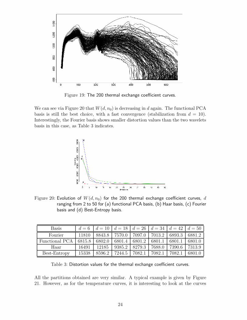
Figure 19: The 200 thermal exchange coefficient curves.
We can see via Figure 20 that W (d, n0) is decreasing in d again. The functional PCAbasis is still the best choice, with a fast convergence (stabilization from d = 10).Interestingly, the Fourier basis shows smaller distortion values than the two waveletsbasis in this case, as Table 3 indicates.
Figure 20: Evolution of W (d, n0) for the 200 thermal exchange coefficient curves, dranging from 2 to 50 for (a) functional PCA basis, (b) Haar basis, (c) Fourierbasis and (d) Best-Entropy basis.
Basis d = 6 d = 10 d = 18 d = 26 d = 34 d = 42 d = 50
Fourier 11810 8843.8 7570.0 7097.0 7013.2 6893.3 6881.2Functional PCA 6815.8 6802.0 6801.4 6801.2 6801.1 6801.1 6801.0
Haar 16491 12185 9385.2 8279.3 7688.0 7390.6 7313.9Best-Entropy 15338 8596.2 7244.5 7082.1 7082.1 7082.1 6801.0
Table 3: Distortion values for the thermal exchange coefficient curves.
All the partitions obtained are very similar. A typical example is given by Figure21. However, as for the temperature curves, it is interesting to look at the curves
24

selected as centers. Figure 22 shows the three centers obtained with the Fourierbasis, functional PCA basis, Haar basis and Best-Entropy basis, for d = 30.
Figure 21: Three clusters obtained with d = 14, functional PCA basis.
a) b)
c) d)
Figure 22: The three centers with (a) Fourier, (b) functional PCA, (c) Haar and (d)Best-Entropy basis, for d = 30.
5 Conclusion
These clusters allow to build accurate models for the industrial application. Thepartitioning method presented in this article has been integrated in our metamodelwritten in R. More specifically, given an array of n input vectors corresponding to noutput curves, the purpose is to learn a function φ : z 7→ x mapping an input vectorto a continuous curve. In order to improve the accuracy of this task, we begin with
25

a clustering step and then look for a regression model in each cluster separately.The metamodel lets the user choose between several clustering techniques, eitherassuming some clusters shapes (like this projected k-means) or trying to discoverthem in data (like the ascendant hierarchical clustering). The latter are attractiveas they do not make assumptions about the results, but they generally need arelatively good sampling of the data. Consequently, the k-means-like techniques areuseful in many of our industrial applications, where only a few samples are available.Moreover, these methods provide easily interpretable clusters. In each cluster, aftera dimension reduction step, which can either be achieved through the decompositionon an orthonormal basis (linear), or any manifold learning algorithm (nonlinear, withthe assumption that the outputs lie on a functional manifold), a statistical learningmethod is applied to predict representation within this cluster. The mainly usedmethod at this stage is the Projection Pursuit Regression algorithm (see Friedman,Jacobson, and Stuetzle [16]). Finally, a simple k-nearest neighbors classifier givesthe most probable cluster for a new input, the corresponding regression function isapplied, and the curve can be reconstruct from its predicted representation.
For the moment, our metamodel with the clustering method presented have success-fully been used on two different scenarios involving the CATHARE code (minor ormajor break, for each we get temperature, pressure and thermal exchange coefficientcurves).
Another research track could consist in considering other types of distances be-tween curves. Distances involving derivatives might be hard to estimate on thethermal exchange coefficient dataset, because several curves are varying rapidlyover short period of time, contrasting for instance with the Tecator dataset (http:
//lib.stat.cmu.edu/datasets/tecator), on which such distances proved success-ful (Ferraty and Vieu [15, Chapter 8], Rossi and Villa [34]). However, further inves-tigations are needed to know if a smoothing step before clustering based on m-orderderivatives would lead to improved results. As the “true” classes are unknown, sucha procedure can only be validated within a cross validation framework involvingthe full metamodel. Experiments with the L1 distance or some mixed distances re-lated to functions shapes (Heckman and Zamar [22]) could also be studied in futureresearch.
26

6 Proofs
6.1 Proof of Lemma 2.1
If we define the remainder Rd by Rd(x) = x − Πd(x) for all x ∈ S, then for(x,y) ∈ S2,
‖Rd(x− y)‖2 ≤ 2‖Rd(x)‖2 + 2‖Rd(y)‖2
= 2+∞∑
j=d
x2j + 2
+∞∑
j=d
y2j
= 2+∞∑
j=d
ϕjx2j
ϕj+ 2
+∞∑
j=d
ϕjy2j
ϕj
(ϕj > 0 for all j ≥ d, since d > j0)
≤ 2+∞∑
j=d
ϕjx2j
ϕd+ 2
+∞∑
j=d
ϕjy2j
ϕd
≤ 4R2
ϕd.
Thus, for c ∈ Sk,
W∞(c)−Wd(c) = E
[
min`=1,...,k
‖X − c`‖2 − min`=1,...,k
‖Πd(X)− Πd(c`)‖2]
= E
[
min`=1,...,k
‖Πd(X) +Rd(X)− Πd(c`)− Rd(c`)‖2
− min`=1,...,k
‖Πd(X)−Πd(c`)‖2]
= E
[
min`=1,...,k
(
‖Πd(X)− Πd(c`)‖2 + ‖Rd(X)− Rd(c`)‖2)
− min`=1,...,k
‖Πd(X)−Πd(c`)‖2]
(since Πd is the orthogonal projection on Rd)
≤ E
[
max`=1,...,k
‖Rd(X)− Rd(c`)‖2]
≤ 4R2
ϕd.
Hence,
supc∈Sk
[W∞(c)−Wd(c)] ≤ 4R2
ϕd,
as desired.
6.2 Proof of Theorem 2.1
We have
W∞(cd,n)−W ∗∞ = W∞(cd,n)−Wd(cd,n) +Wd(cd,n)−W ∗d +W ∗d −W ∗∞.
27

According to Lemma 2.1, on the one hand,
W∞(cd,n)−Wd(cd,n) ≤ supc∈Sk
[W∞(c)−Wd(c)]
≤ 4R2
ϕd,
and on the other hand,
W ∗d −W ∗∞ = infc∈Sk
Wd(c)− infc∈Sk
W∞(c)
≤ supc∈Sk
[W∞(c)−Wd(c)]
≤ 4R2
ϕd,
and the theorem is proved.
References
[1] C. Abraham, P. A. Cornillon, E. Matzner-Løber, and N. Molinari. UnsupervisedCurve Clustering using B-Splines. Scandinavian Journal of Statistics, 30:581–595, 2003.
[2] R. J. Alcock and Y. Manolopoulos. Time-series similarity queries employing afeature-based approach. In 7th Hellenic Conference on Informatics, Ioannina,Greece, 1999.
[3] A. Antoniadis, X. Brossat, J. Cugliari, and J-M. Poggi. Clustering functionaldata with wavelets. In Y. Lechevallier and G. Saporta, editors, e-Book COMP-STAT 2010, pages 697–704. Springer, 2010.
[4] N. Aronszajn. Theory of reproducing kernel. Transactions of American Math-ematical Society, 68:337–404, 1950.
[5] B. Auder, A. De Crecy, B. Iooss, and M. Marquès. Screening and metamodel-ing of computer experiments with functional outputs. Application to thermal-hydraulic computations. http://hal.archives-ouvertes.fr/docs/00/52/
54/91/PDF/ress_samo10_BA.pdf.
[6] G. Biau, L. Devroye, and G. Lugosi. On the performance of clustering in Hilbertspaces. IEEE Transactions on Information Theory, 2008.
[7] J. M. Chiou and P. L. Li. Functional Clustering of Longitudinal Data. InS. Dabo-Niang and F. Ferraty, editors, Functional and Operatorial Statistics,Contributions to Statistics, chapter 17, pages 103–107. Physica-Verlag, Heidel-berg, 2008.
[8] A. Cohen, I. Daubechies, and P. Vial. Wavelets on the interval and fast wavelettransforms. Applied and Computational Harmonic Analysis, 1:54–81, 1993.
28

[9] R. R. Coifman and M. V. Wickerhauser. Entropy-based algorithms for bestbasis selection. IEEE Transactions on Information Theory, 38:713–718, 1992.
[10] F. Cucker and S. Smale. On the mathematical foundations of learning. Bulletinof the American Mathematical Society, 39:1–49, 2002.
[11] I. Daubechies. Ten Lectures on Wavelets. Society for Industrial and AppliedMathematics, Philadelphia, 1992.
[12] R. A. DeVore and G. G. Lorentz. Constructive Approximation. Springer-Verlag,Berlin, 1993.
[13] D. L. Donoho and I. M. Johnstone. Minimax estimation via wavelet shrinkage.Annals of Statistics, 26:879–921, 1998.
[14] R. O. Duda, P. E. Hart, and D. G. Stork. Pattern Classification. Wiley-Interscience, New York, second edition, 2000.
[15] F. Ferraty and P. Vieu. Nonparametric Functional Data Analysis: Theory andPractice. Springer Series in Statistics. Springer-Verlag, New York, 2006.
[16] J. H. Friedman, M. Jacobson, and W. Stuetzle. Projection pursuit regression.Journal of the American Statistical Association, 76:817–846, 1981.
[17] S. Gaffney. Probabilistic Curve-Aligned Clustering and Prediction with MixtureModels. PhD thesis, Department of Computer Science, University of Califor-nia, Irvine, 2004. http://www.ics.uci.edu/~sgaffney/papers/sgaffney_
thesis.pdf.
[18] A. Gersho and R. M. Gray. Vector Quantization and Signal Compression.Kluwer Academic Publishers, Norwell, 1992.
[19] R. G. Ghanem and P. D. Spanos. Stochastic Finite Elements: A Spectral Ap-proach. Springer-Verlag, New York, 1991.
[20] A. D. Gordon. Classification. Monographs on Statistics and Applied Probabil-ity. Chapman and Hall/CRC, London, second edition, 1999.
[21] S. Graf and H. Luschgy. Foundations of Quantization for Probability Distribu-tions. Lecture Notes in Mathematics. Springer-Verlag, Berlin, 2000.
[22] N.E. Heckman and R.H. Zamar. Comparing the shapes of regression functions.Biometrika, 87:135–144, 2000.
[23] G. M. James and C. A. Sugar. Clustering for sparsely sampled functional data.Journal of the American Statistical Association, 98:397–408, 2003.
[24] T. Linder. Learning-Theoretic Methods in Vector Quantization. In L. Györfi,editor, Principles of Nonparametric Learning, CISM lecture Notes. Springer,Wien, New York, 2002.
29

[25] S. P. Lloyd. Least squares quantization in PCM. IEEE Transactions on Infor-mation Theory, 28:129–137, 1982.
[26] W. L. Loh. On latin hypercube sampling. The Annals of Statistics, 24:2058–2080, 1996.
[27] S. Mallat. A wavelet tour of signal processing, The Sparse Way. AcademicPress, Burlington, third edition, 2009.
[28] M. D. McKay, W. J. Conover, and R. J. Beckman. A comparison of threemethods for selecting values of input variables in the analysis of output from acomputer code. Technometrics, 21:239–245, 1979.
[29] N. Merhav and J. Ziv. On the amount of statistical side information requiredfor lossy data compression. IEEE Transactions on Information Theory, 43,1997.
[30] Y. Meyer. Wavelet and Operators. Cambridge University Press, Cambridge,1992.
[31] G. W. Milligan and M. C. Cooper. An examination of procedures for determin-ing the number of clusters in a data set. Psychometrika, 50:159–79, 1985.
[32] J. O. Ramsay and B. W. Silverman. Functional Data Analysis. Springer, NewYork, second edition, 2006.
[33] F. Rossi, B. Conan-Guez, and A. El Golli. Clustering functional data withthe som algorithm. In ESANN’2004 proceedings - European Symposium onArtificial Neural Networks, pages 305–312, Bruges (Belgium), 28-30 April 2004.
[34] F. Rossi and N. Villa. Support vector machine for functional data classification.Neurocomputing, 69:730–742, 2006.
[35] A. B. Tsybakov. On the best rate of adaptive estimation in some inverse prob-lems. Comptes-rendus de l’Académie des Sciences, Paris, 2000.
[36] A. B. Tsybakov. Introduction to Nonparametric Estimation. Springer Series inStatistics. Springer, New York, 2009.
[37] M. V. Wickerhauser. Adapted Wavelet Analysis from Theory to Software. A. K.Peters/CRC Press, Wellesley, 1996.
[38] R. C. Williamson, A. J. Smola, and B. Schölkopf. Generalization performanceof regularization networks and support vector machines via entropy numbers ofcompact operators. IEEE Transactions on Information Theory, 47:2516–2532,2001.
30