project: wireless sensor network for smartgrid applications
TRANSCRIPT

PROJECT: Wireless Sensor Network for SmartgridApplications
(Rede de Sensores sem Fios para Aplicacoes de Smartgrid)
Joao Pedro Taveira Pinto da Silva
Thesis to obtain the Master of Science Degree in
Information Systems and Computer Engineering
Supervisors: Prof. Rui Antonio dos Santos CruzDr. Berend Willem Martijn Kuipers
Examination Committee
Chairperson: Prof. Daniel Jorge Viegas GoncalvesSupervisor: Prof. Rui Antonio dos Santos Cruz
Member of the Committee: Prof. Alberto Manuel Ramos da Cunha
October 2017


Acknowledgments
Acknowledgements
The author would like to thank his supervisors Prof. Mario Serafim Nunes and Prof. Rui Cruz, his
external advisor and colleague Martijn Kuipers and his other colleagues at Inesc Inovacao (INOV) for
the fruitful cooperation and pleasant working environment.


Abstract
The use of voltage and current control in the Low Voltage grid has become indispensable to the Distribu-
tion System Operator in order to manage the grid. The e-Balance project, an EU funded project, focused
on this challenge. This work was executed as part of the e-Balance project and the author developed
the software for a wireless approach to Low Voltage grid monitoring.
Communication between the data collector and the Wireless Sensor Network nodes is based on
DLMS using logical name references, which is the most common used standard for energy monitoring.
In this work a novel implementation of a specification compliant DLMS/COSEM server is implemented
with a focus on low resource usage.
The author proposed to use the Contiki OS running on a low-cost Atmega Microcontroller Unit with
at least 128kB of flash for the Wireless Mesh Node. The author also proposed to use a commercially
of the shelf OpenWRT capable device for the Wireless Mesh Gateway, adapted to use with the XBee
transceivers.
The performance of the Wireless Sensor Network was considered very good, taking into account
the foreseen applications and a success rate higher than 99% was obtained. Three different sensor
configurations are supported, using the same code-base. In this work, 51 information objects were
implemented using 7 different classes.
The developed system was evaluated for a prolonged period in a realistic test-bed installed in the
Batalha region of Portugal and obtained very good feedback and praise from the project reviewers.
Keywords
smartgrid; sensorization; wireless mesh networks; DLMS; COSEM; RPL; 6LowPAN
iii


Resumo
O uso de mecanismos de controlo do nıvel de tensao e fluxo de corrente em redes de distribuicao de
electricidade tem-se mostrado indispensaveis para a gestao de operacao dos operadores de distribuicao.
O Projecto e-Balance, co-financiado pela Uniao Europeia, enquadra-se neste desafio, sendo o trabalho
apresentado neste relatorio parte deste projecto, tendo sido o autor responsavel por desenvolver um
sistema informatico de monitorizacao da rede electrica de baixa tensao, usando como base uma rede
de sensores sem fios.
Visando normas de troca de informacao amplamente adoptadas pela industria, a troca de informacao
entre sensores e sistemas de monitorizacao e feita usando protocolo DLMS/COSEM. Neste trabalho e
apresentada uma implementacao de servidor deste protocolo, tendo em conta restricoes de utilizacao
de memoria e baixo consumo de sensores.
Foi proposto pelo autor a utilizacao de um processador de baixo custo, usando a plataforma Con-
tiki, para suporte a rede de sensores. Para a Gateway de rede sem fios foi proposto pelo autor um
dispositivo baseado no OpenWRT, que permite adaptacao e utilizacao de modulos de comunicacoes
XBee.
A avaliacao da performance da rede sem fios demonstrou resultados muito positivos, atingindo
disponibilidades da rede de 99%. O codigo base desenvolvido suporta tres versoes diferentes de sen-
sores e implementa 51 diferentes indicadores informativos de 7 classes distintas.
O sistema desenvolvido foi avaliado durante um longo perıodo de tempo num ambiente real instalado
na regiao da Batalha, em Portugal. O projecto foi avaliado muito positivamente da parte da comissao
avaliadora da Comissao Europeia.
v

Palavras Chave
redes inteligentes; monitorizacao; redes de sensores sem fios; DLMS; COSEM; RPL; 6LowPAN
vi

Contents
1 Introduction 1
1.1 e-Balance Objective: a Portuguese perspective . . . . . . . . . . . . . . . . . . . . . . . . 1
1.2 Overall architecture of the e-Balance LV Grid Monitor Solution . . . . . . . . . . . . . . . . 2
1.3 System Components Analysis . . . . . . . . . . . . . . . . . . . . . . . . . . . . . . . . . . 3
1.3.1 Sensorization of the LV Grid . . . . . . . . . . . . . . . . . . . . . . . . . . . . . . . 4
1.3.2 LV Grid Fault Detection and Location . . . . . . . . . . . . . . . . . . . . . . . . . . 5
1.4 Contributed Work . . . . . . . . . . . . . . . . . . . . . . . . . . . . . . . . . . . . . . . . . 6
2 System Requirements 7
2.1 Data Acquisition and Control . . . . . . . . . . . . . . . . . . . . . . . . . . . . . . . . . . 7
2.2 Networking . . . . . . . . . . . . . . . . . . . . . . . . . . . . . . . . . . . . . . . . . . . . 8
2.3 Sensing . . . . . . . . . . . . . . . . . . . . . . . . . . . . . . . . . . . . . . . . . . . . . . 9
2.4 Reliability . . . . . . . . . . . . . . . . . . . . . . . . . . . . . . . . . . . . . . . . . . . . . 9
2.5 Hardware Platforms . . . . . . . . . . . . . . . . . . . . . . . . . . . . . . . . . . . . . . . 10
2.5.1 Sensor node . . . . . . . . . . . . . . . . . . . . . . . . . . . . . . . . . . . . . . . 10
2.5.2 Sensor Base Firmware . . . . . . . . . . . . . . . . . . . . . . . . . . . . . . . . . 10
2.5.3 Wireless Mesh Gateway . . . . . . . . . . . . . . . . . . . . . . . . . . . . . . . . . 11
3 Technical Specification 13
3.1 Design Goals and Principles . . . . . . . . . . . . . . . . . . . . . . . . . . . . . . . . . . 14
3.2 System Overview . . . . . . . . . . . . . . . . . . . . . . . . . . . . . . . . . . . . . . . . . 14
3.3 Network Architecture . . . . . . . . . . . . . . . . . . . . . . . . . . . . . . . . . . . . . . . 14
3.4 Acquisition and Control . . . . . . . . . . . . . . . . . . . . . . . . . . . . . . . . . . . . . 16
3.4.1 DLMS . . . . . . . . . . . . . . . . . . . . . . . . . . . . . . . . . . . . . . . . . . . 16
3.4.2 CoAP . . . . . . . . . . . . . . . . . . . . . . . . . . . . . . . . . . . . . . . . . . . 16
3.5 Mesh Network . . . . . . . . . . . . . . . . . . . . . . . . . . . . . . . . . . . . . . . . . . 17
3.5.1 Network stack . . . . . . . . . . . . . . . . . . . . . . . . . . . . . . . . . . . . . . 17
3.5.2 Availability and Synchronisation . . . . . . . . . . . . . . . . . . . . . . . . . . . . . 17
3.5.3 Pilot related network considerations . . . . . . . . . . . . . . . . . . . . . . . . . . 18
vii

3.6 Sensing Mechanisms . . . . . . . . . . . . . . . . . . . . . . . . . . . . . . . . . . . . . . 18
3.7 Hardware Characteristics . . . . . . . . . . . . . . . . . . . . . . . . . . . . . . . . . . . . 20
3.7.1 Sensing Node . . . . . . . . . . . . . . . . . . . . . . . . . . . . . . . . . . . . . . 20
3.7.2 Wireless Mesh Gateway . . . . . . . . . . . . . . . . . . . . . . . . . . . . . . . . . 21
4 System Implementation 25
4.1 Sensing Modules . . . . . . . . . . . . . . . . . . . . . . . . . . . . . . . . . . . . . . . . . 26
4.1.1 modbus Driver . . . . . . . . . . . . . . . . . . . . . . . . . . . . . . . . . . . . . . 26
4.1.2 LV Sensor . . . . . . . . . . . . . . . . . . . . . . . . . . . . . . . . . . . . . . . . . 26
4.1.3 Fault Detector Driver . . . . . . . . . . . . . . . . . . . . . . . . . . . . . . . . . . . 28
4.2 Networking Modules . . . . . . . . . . . . . . . . . . . . . . . . . . . . . . . . . . . . . . . 28
4.2.1 XBee Communication Transceiver Driver . . . . . . . . . . . . . . . . . . . . . . . 28
4.2.2 TimeSync: NTP reference broadcast and RPL Parent Probing . . . . . . . . . . . 29
4.2.3 3G Connection Checker . . . . . . . . . . . . . . . . . . . . . . . . . . . . . . . . . 29
4.2.4 pingstats . . . . . . . . . . . . . . . . . . . . . . . . . . . . . . . . . . . . . . . . . 30
4.2.5 meshstats . . . . . . . . . . . . . . . . . . . . . . . . . . . . . . . . . . . . . . . . . 30
4.2.6 Network Event Notifications . . . . . . . . . . . . . . . . . . . . . . . . . . . . . . . 30
4.3 DLMS/COSEM Server . . . . . . . . . . . . . . . . . . . . . . . . . . . . . . . . . . . . . . 31
4.3.1 Requirements related choices . . . . . . . . . . . . . . . . . . . . . . . . . . . . . . 31
4.3.2 Implemented Classes and OBIS Lists . . . . . . . . . . . . . . . . . . . . . . . . . 31
4.3.3 Considerations related to Server Program Code . . . . . . . . . . . . . . . . . . . 40
4.4 CoAP Services . . . . . . . . . . . . . . . . . . . . . . . . . . . . . . . . . . . . . . . . . . 43
4.5 Wireless Flash . . . . . . . . . . . . . . . . . . . . . . . . . . . . . . . . . . . . . . . . . . 50
5 System Validation 53
5.1 Hardware Appliance Robustness and Reliability Evaluation . . . . . . . . . . . . . . . . . 53
5.1.1 Reliability: graceful and non-graceful reboot tests . . . . . . . . . . . . . . . . . . . 53
5.1.2 Diagnostics Self-test and Calibration . . . . . . . . . . . . . . . . . . . . . . . . . . 55
5.1.3 Appliance power failure mechanisms tests . . . . . . . . . . . . . . . . . . . . . . . 55
5.1.4 Gateway WAN Connectivity tests . . . . . . . . . . . . . . . . . . . . . . . . . . . . 57
5.2 System Performance and Availability Evaluation . . . . . . . . . . . . . . . . . . . . . . . . 57
5.2.1 Mesh Stats Analysis . . . . . . . . . . . . . . . . . . . . . . . . . . . . . . . . . . . 58
5.2.2 Measurements Availability . . . . . . . . . . . . . . . . . . . . . . . . . . . . . . . . 58
5.3 Demonstrator Operation System Evaluation . . . . . . . . . . . . . . . . . . . . . . . . . . 60
6 Conclusion 67
viii

A MonitorBT: Survey on communications technologies 77
A.1 PLC . . . . . . . . . . . . . . . . . . . . . . . . . . . . . . . . . . . . . . . . . . . . . . . . 80
A.2 Infrastructure-based Wireless Networks . . . . . . . . . . . . . . . . . . . . . . . . . . . . 81
A.3 RF-Mesh . . . . . . . . . . . . . . . . . . . . . . . . . . . . . . . . . . . . . . . . . . . . . 83
A.4 Summary . . . . . . . . . . . . . . . . . . . . . . . . . . . . . . . . . . . . . . . . . . . . . 87
B Bandwidth Estimation Tests 89
B.1 Procedure 1: Ping-test . . . . . . . . . . . . . . . . . . . . . . . . . . . . . . . . . . . . . . 89
B.2 Procedure 2: Differential Ping-test . . . . . . . . . . . . . . . . . . . . . . . . . . . . . . . 90
C Code 91
C.1 Non-graceful Reboot Test Script . . . . . . . . . . . . . . . . . . . . . . . . . . . . . . . . 91
C.2 Complete List of COSEM objects . . . . . . . . . . . . . . . . . . . . . . . . . . . . . . . . 94
D DLMSWeb 99
ix

x

List of Figures
1.1 Overall architecture of the e-Balance. . . . . . . . . . . . . . . . . . . . . . . . . . . . . . 3
3.1 System Overview in e-Balance Architecture . . . . . . . . . . . . . . . . . . . . . . . . . . 15
3.2 System Overview Block Diagram . . . . . . . . . . . . . . . . . . . . . . . . . . . . . . . . 15
3.3 System Wireless Network Stack. . . . . . . . . . . . . . . . . . . . . . . . . . . . . . . . . 17
3.4 Network Stack between WMG and INOV networks. . . . . . . . . . . . . . . . . . . . . . . 18
3.5 iBee Block Diagram . . . . . . . . . . . . . . . . . . . . . . . . . . . . . . . . . . . . . . . 19
3.6 Wireless Mesh Gateway Block Diagram . . . . . . . . . . . . . . . . . . . . . . . . . . . . 22
4.1 Voltages Thresholds . . . . . . . . . . . . . . . . . . . . . . . . . . . . . . . . . . . . . . . 27
4.2 Currents Thresholds . . . . . . . . . . . . . . . . . . . . . . . . . . . . . . . . . . . . . . . 27
4.3 Wireless Flash Sequence Diagram . . . . . . . . . . . . . . . . . . . . . . . . . . . . . . . 51
5.1 Test reboot: Root Node (Sensor 5c60) . . . . . . . . . . . . . . . . . . . . . . . . . . . . . 54
5.2 Test reboot: Leaf #1 (Sensor c99d) . . . . . . . . . . . . . . . . . . . . . . . . . . . . . . . 54
5.3 Test reboot: Leaf #2 (Sensor c95a) . . . . . . . . . . . . . . . . . . . . . . . . . . . . . . . 54
5.4 Test reboot: Leaf #3 (Sensor c999) . . . . . . . . . . . . . . . . . . . . . . . . . . . . . . . 55
5.5 Gateway update 6in4 endpoints service . . . . . . . . . . . . . . . . . . . . . . . . . . . . 58
5.6 Gateway Mesh Nodes: Overview web page . . . . . . . . . . . . . . . . . . . . . . . . . . 59
5.7 Measurements Availability May 2017 . . . . . . . . . . . . . . . . . . . . . . . . . . . . . . 59
5.8 Monitoring the LV grid (comprising public lighting) in Golpilheira . . . . . . . . . . . . . . . 61
5.9 Monitoring the LV grid in Jardoeira . . . . . . . . . . . . . . . . . . . . . . . . . . . . . . . 62
5.10 Layout of the main project units serving a secondary substation . . . . . . . . . . . . . . . 63
5.11 Close-up of a gateway . . . . . . . . . . . . . . . . . . . . . . . . . . . . . . . . . . . . . . 64
5.12 Deployment of a 3-phase sensor in a pole . . . . . . . . . . . . . . . . . . . . . . . . . . . 65
5.13 Close-up of a 3-phase sensor in a pole . . . . . . . . . . . . . . . . . . . . . . . . . . . . . 65
6.1 Internals of the Wireless Mesh Node . . . . . . . . . . . . . . . . . . . . . . . . . . . . . . 69
xi

6.2 Internals of the Wireless Mesh Gateway . . . . . . . . . . . . . . . . . . . . . . . . . . . . 69
6.3 Demonstrator with the secondary substation at Golpilheira . . . . . . . . . . . . . . . . . . 70
6.4 Demonstrator with the secondary substation at Jardoeira . . . . . . . . . . . . . . . . . . 70
A.1 InovGrid System Architecture. . . . . . . . . . . . . . . . . . . . . . . . . . . . . . . . . . . 78
D.1 DLMS Web LV Grid . . . . . . . . . . . . . . . . . . . . . . . . . . . . . . . . . . . . . . . 100
D.2 DLMS Web Wireless Mesh Node interface . . . . . . . . . . . . . . . . . . . . . . . . . . . 100
xii
List of Tables
4.1 Data (class id: 1, version: 0) . . . . . . . . . . . . . . . . . . . . . . . . . . . . . . . . . . 32
4.2 Register (class id: 3, version: 0) . . . . . . . . . . . . . . . . . . . . . . . . . . . . . . . . 33
4.3 Demand Register (class id: 5, version: 0) . . . . . . . . . . . . . . . . . . . . . . . . . . . 33
4.4 Profile Generic (class id: 7, version: 1) . . . . . . . . . . . . . . . . . . . . . . . . . . . . . 34
4.5 Association LN (class id: 15, version: 2) . . . . . . . . . . . . . . . . . . . . . . . . . . . . 35
4.6 Sensor Manager (class id: 67, version: 0) . . . . . . . . . . . . . . . . . . . . . . . . . . . 36
4.7 Extended Register (class id: 4, version: 0) . . . . . . . . . . . . . . . . . . . . . . . . . . . 37
4.8 Register Monitor (class id: 21, version: 0) . . . . . . . . . . . . . . . . . . . . . . . . . . . 38
4.9 Firmware sizes . . . . . . . . . . . . . . . . . . . . . . . . . . . . . . . . . . . . . . . . . . 42
4.10 Get Firmware Release Version and build date CoAP Service . . . . . . . . . . . . . . . . 43
4.11 Reset/Erase persistent data from sensor modules CoAP Service . . . . . . . . . . . . . . 43
4.12 Force Non-graceful Reboot of the sensor CoAP Service . . . . . . . . . . . . . . . . . . . 44
4.13 Get Radio module statistics CoAP Service . . . . . . . . . . . . . . . . . . . . . . . . . . . 44
4.14 Set radio module transmit power CoAP Service . . . . . . . . . . . . . . . . . . . . . . . . 44
4.15 Trigger DLMS/COSEM Event Notification CoAP Service . . . . . . . . . . . . . . . . . . . 45
4.16 Get LV Sensor calibration parameters CoAP Service . . . . . . . . . . . . . . . . . . . . . 46
4.17 Set LV Sensor calibration parameters CoAP Service . . . . . . . . . . . . . . . . . . . . . 47
4.18 Get Current Fault Detector calibration parameters CoAP Service . . . . . . . . . . . . . . 48
4.19 Set Current Fault Detector calibration parameters CoAP Service . . . . . . . . . . . . . . 49
4.20 Trigger RF-Mesh topology re-establishment (RPL repair) CoAP Service . . . . . . . . . . 50
5.1 Reboot Test Time Results . . . . . . . . . . . . . . . . . . . . . . . . . . . . . . . . . . . . 54
5.2 Self Test and Calibration Check-list . . . . . . . . . . . . . . . . . . . . . . . . . . . . . . . 56
5.3 Measurements Availability Results . . . . . . . . . . . . . . . . . . . . . . . . . . . . . . . 60
A.1 Comparison between Smart Grid Local Area Network (LAN) communication Technologies 87
xiii

xiv

List of Listings
4.1 Example of COSEM objects list definition . . . . . . . . . . . . . . . . . . . . . . . . . . . 41
4.2 Example of COSEM objects list instantiation . . . . . . . . . . . . . . . . . . . . . . . . . . 41
4.3 Example of IC1 get attribute function . . . . . . . . . . . . . . . . . . . . . . . . . . . . . . 42
C.1 Non-graceful Reboot test script . . . . . . . . . . . . . . . . . . . . . . . . . . . . . . . . . 93
C.2 Complete list of COSEM objects definition . . . . . . . . . . . . . . . . . . . . . . . . . . . 98
xv

xvi

Acronyms
2G 2nd Generation
3G 3rd Generation
6LoWPAN IPv6 over Low power WPAN
AA Application Association
AMR Automatic Meter Reading
AMR Automatic Meter Reading
AODV Ad-hoc On-Demand Distance Vector
ARIB Association of Radio Industries and Businesses
AVR modified Harvard architecture 8-bit RISC single-chip microcontroller
BAA Building Automation Applications
BB Broadband
BGA Ball Grid Array
BPL Broadband Over Power Line
CENELEC European Committee for Electrotechnical Standardization
CEPRI China’s Electric Power Research Institute
CIM Common Information Model
COSEM Companion Specification for Energy Metering
CSMA/CA Carrier Sense Multiple Access with Collision Avoidance
DCSK Differential Chaos Shift Keying
xvii

DER Distributed Energy Resources
DLMS Device Language Message Specification
DMS Distribution Management System
DODAGs Destination Oriented Directed Acyclic Graphs
DSO Distribution System Operator
DSSS Direct-Sequence Spread Spectrum
DTC Distribution Transformer Controllers
EB Energy Box
EDC Electric Distribution Cabinets
EEPROM Electrically Erasable Programmable Read-Only Memory
EPC Electric Protection Cabinets
ETX Expected Number of Transmissions
EUTC European Utilities Telecom Council
FCC Federal Communications Commission
FHSS Frequency Hop Spread Spectrum
GPRS General Packet Radio Service
GPRS General Packet Radio Service
GSM Global System for Mobile Communications
GSM Global System for Mobile Communications
HAN Home Area Network
HF High Frequency
HSDPA High-Speed Downlink Packet Access
HSUPA High-Speed Uplink Packet Access
HV High Voltage
HWMP Hybrid Wireless Mesh Protocol
xviii

IC Integrated Circuit
ICs Interface classes
ICMP Internet Control Message Protocol
ICT Information and Communication Technologies
IEC International Electrotechnical Commission
IETF Internet Engineering Task Force
INOV Inesc Inovacao
IP Internet Protocol
IPv4 Internet Protocol version 4
IPv6 Internet Protocol version 6
ISA International Society for Automation
ISM Industrial, Scientific and Medical
ITU International Telecommunication Union
IoT Internet-of-Things
LAN Local Area Network
LF Low Frequency
LLNs Low Power and Lossy Networks
LoS Line of Sight
LQFP Low profile Quad Flat Pack
LTE Long-Term Evolution
LV Low Voltage
MAC Media Access Control
MCU Microcontroller Unit
MIMO multiple-input and multiple-output
MTU Maximum Transmission Unit
xix

MV Medium Voltage
NB Narrowband
NIST National Institute of Standards and Technology
NTP Network Time Protocol
OBIS OBject Identification System
OFDM Orthogonal Frequency Division Multiplexing
OFDMA Orthogonal Frequency Division Multiple Access
PDU Protocol Data Unit
PEV Plug-in Electric Vehicle
PHY Physical Layer Protocol
PL public lighting
PLC Power Line Communications
PLMN Public Land Mobile Network
PRIME PoweRline Intelligent Metering Evolution
PV Photovoltaic
QoS Quality Of Service
RAM Random-Access Memory
RF Radio-frequency
RF-Mesh Radio-frequency Mesh
ROLL Routing Over Low power and Lossy networks
RPL Routing Protocol for Low-Power and Lossy Networks
RTT round-trip time
S-FSK Spread Frequency Shift Keying
SC-FDMA Single-Carrier Frequency Division Multiple Access
SCADA Supervisory Control and Data Acquisition
xx

SLIP Serial Line Internet Protocol
SPI Serial Peripheral Interface
SSC Smart Substation Controller
SUN Smart Utility Networks
SoC System-On-Chip
TCP Transport Control Protocol
TDMA Time Division Multiple Access
TETRA Terrestrial Trunked Radio
TTL Time-to-Live
UART Universal Asynchronous Receiver-Transmitter
UDP User Datagram Protocol
UHF Ultra-High Frequency
UMTS Universal Mobile Telecommunications System
UMTS Universal Mobile Telecommunication System
UNB Ultra Narrowband
VHF Very High Frequency
VLF Very Low Frequency
WAN Wide Area Network
WLAN Wireless Local Area Network
WMG Wireless Mesh Gateway
WMN Wireless Mesh Nodes
WSN Wireless Sensor Network
µG micro-generation
xxi

xxii
1Introduction
The work presented in this document corresponds to components of a European Union funded
project named “e-Balance”, a European funded project with several international partners [1]. The work
of the author at Inesc Inovacao (INOV) was focused on the wireless sensor nodes developed in the
project by INOV. The e-Balance project is the international follow-up to the Monitor BT project, which
allowed to develop an improved wireless sensor based on the Monitor BT sensor also developed by the
author.
The developed devices and fault detection and location functionalities are to be integrated in a pilot
Grid area of EDP Distribuicao (the Portuguese Distribution System Operator (DSO)) in the region of
Batalha, Portugal, whose infrastructure provides a realistic demonstrator for validating the solution.
1.1 e-Balance Objective: a Portuguese perspective
The Smart Grid concept is innovative concerning the use of Information and Communication Tech-
nologies (ICT) in the management and control of the electric power grid, including all of its grid segments:
generation, transmission, distribution and consumption. According to this concept, the Smart Grid will
1
provide features, such as integration of micro-producers (which may also be consumers), automatic fault
detection and service restoration, and the reconfiguration of the grid according to the energy offer/de-
mand at each instant.
These features require the electric power grid to be sensorized first (i.e., integrate sensors for relevant
measuring of the electric power grid state with the systems responsible for its processing). Furthermore,
the grid has to incorporate electro-mechanic actuators, which are used for grid reconfiguration. Due to
the dimension of the grid infrastructure already installed, a gradual evolution from the traditional grid to
the Smart Grid is expected.
At the lower end, the Low Voltage (LV) network currently has a passive character due to the lack of
suitable equipment to allow gathering of information on the infrastructure’s operational status, as well as
to allow any kind of remote actuation. Currently there is motivation for the deployment of smart meters
and communication interfaces up to costumer’s equipment level in the context of Smart Grids. Based on
these trends, there is an opportunity to research and develop a set of advanced monitoring and control
functionalities for the LV network, which are currently associated with the concept of the Smart Grid.
Operational data collected along the LV feeders by wireless meshed sensors enable fault detection
and location, as well as fuse-blown detection in distribution cabinets and in secondary substations,
leading to a reduction on LV grid downtime, improving Quality Of Service (QoS).
Furthermore, last-gasp alarms from sensors allow the management system to react faster, improving
maintenance teams response.
1.2 Overall architecture of the e-Balance LV Grid Monitor Solution
Figure 1.1 presents the overall architecture of the e-Balance LV Grid Monitor Solution. This architec-
ture matches smart grid requirements as it copes with distributed monitoring and control, by including
open communication protocols deployed over proven Radio-frequency Mesh (RF-Mesh) and Power Line
Communications (PLC)1. The mentioned criterion arises from the intention to cope with the require-
ments of EDP Distribuicao (the Portuguese distribution system operator), as stated in all EDP’s InovGrid
projects. EDP hosted a real pilot demonstrator - to be deployed within the “e-Balance” project - in its
LV distribution grid, in the region of Batalha. This pilot supports communications (Device Language
Message Specification (DLMS) protocol over RF-Mesh) between master units and their sensor devices,
supporting fault detection and location in the LV grid and in public lighting feeders. The proposed archi-
tecture also enables the integration of other devices, such as smart meters (communicating via DLMS
over PLC Prime), deployed for consumption or micro-generation (µG) PV stakeholders. These players
didn’t participate in the real pilot demonstrator. Nevertheless, µG power control, a major issue for volt-
1PLC and Photovoltaic (PV) are out of scope of this work.
2

age regulation, was demonstrated in laboratory. The PLC Prime standard - out of scope of this project -
will support the communications between the master units and the smart meters, these bridging the µG
inverter’s controller.
A thorough state-of-the-art survey of the LV grid monitoring systems and technologies was previously
written by the author for the purpose of inclusion in a Monitor BT deliverable. The survey can be found
in Appendix A.
Inverter proprietary
DLMS overRF MESH
DLMS overRF MESH
DLMS overPLC PRIME
DLMS
Modbus
DLMS overPLC PRIME
IEC 60870-5-104Web Services
SCADA/DMS
DTC
Smart Meter(PV)
PV inverter
Smart Meter(home user)
Smart Meter(home user)
PV controller
Public Lighting sensors
DTC
FEATURESIntelligentAlarmManagement
FEATURESPublicLightingManagement-FaultDetectionandLocation-FusedLampss ss
DA sensors
FEATURESLVGridFaultDetection
andLocation
FEATURESPVInjectedPowerControl/
VoltageRegulation
Legend
LV–LowVoltageDA–DistributionAutomationPV–Photovoltaicgenerator
CommunicationLinks
RelatedFeaturesGatewayGway
DA sensors
Figure 1.1: Overall architecture of the e-Balance.
1.3 System Components Analysis
One of the main objectives of the project is to provide from sensors in the Grid, an automatic detec-
tion and localisation of faults in the LV power network. The sensorization of the LV network shall be also
carried out in order to support these functionalities. Highlights shall be given to the activities related with
3

the research and development of the communication network, as well as of advanced algorithms for the
optimisation of LV network operations. The main result of the project shall consist of a joint solution com-
prising equipment and functionalities that shall provide the LV network with intelligence. Other important
results comprise all the deliverables and technical specification documents of the developed modules,
as well as the functional and performance test reports. All developed functionalities were integrated in a
real network whose infrastructure provides the interfaces and information required for the creation of a
realistic scenario for the validation of the implemented solution. It is expected that this solution and the
respective technical specifications shall provide a basis for the development of innovative commercial
products in the context of Smart Grids, which fits the interests of national and international electrical
utility operators.
The results of this project, in line with the “e-Balance” project, is a step toward the accomplishment
of the Smart Grid, aiming at demonstrating a subset of the advanced features already described. As a
global result, prototypes of devices were developed with firmware that meets the main goal, which will
improve the Smart Grid once they enter in their commercial phase.
The sub-goals of the project are to add the following functionalities to the power grid sensors:
• Sensorization of the LV Grid
• LV Grid fault detection and location
These functionalities will be described in more detail in the following subsections.
1.3.1 Sensorization of the LV Grid
The High Voltage (HV) and Medium Voltage (MV) grid sensing and remote control infra-structure is
already significantly developed. Yet, the LV grid sensing and remote control level is reduced and almost
non-existent, except some precise LV zones in Lisbon or Oporto. LV fault detections rely on customer
calls informing EDP Distribuicao about outages and on visual inspections made by routine maintenance
crews. Regarding “e-Balance” project, it aims at bringing active strategies for incident detection and
characterisation. These tasks over the LV grid should be proactive, therefore this work aims at bringing
sensing devices to that segment of the grid so that it would be possible to read grid field data, process
it and identify alarm events related to anomalous behaviour of the LV distribution grid. The sensoriza-
tion and fault detection process over the LV grid equipment and lines would then be more efficient if it
could be performed automatically and remotely, through the inclusion of sensors and appropriate com-
munication modules in LV Electric Protection Cabinets (EPC) and Electric Distribution Cabinets (EDC).
The “e-Balance” sensors would perform measuring of voltage, current, power factor, temperature and
humidity. From software point of view, the development of an efficient communication network able
to interconnect those sensors with the control and monitoring central system (the control centre), via
4

Distribution Transformer Controllers (DTC), is fundamental for the implementation of a sensing solution
for the LV grid. The use of several communication technologies of these sensors brings the need for
their integration, so that a single communication network is the outcome.
Therefore, the LV grid sensorization entails the following tasks:
• Development or adaptation of sensing nodes, so that they become self-powered when possible:
– EPC and EDC sensorization.
• Development of the communication network for sensor node interconnection:
– Selection of the communication technologies. One foresees the evaluation of new devices
featuring new communication standards adequate for the scenarios described above.
– Development of the communication protocols for the sensing infrastructure, including require-
ments for self-configuration, self-healing and safety.
– Planning of the sensing infrastructure coping with the requirements of connectivity between
the DTC, EPC and EDC.
• Development of interfaces between the sensing infrastructure and the DTC, as well as specific
features for the data acquisition and control of those sensors.
1.3.2 LV Grid Fault Detection and Location
As already stated, fault detection and location in the LV grid is still inefficient due to the lack of LV grid
sensorization. The latter will enable the automation of the fault detection and location, sending alarm
notifications once a fault is impending or detected. Existing mechanisms for polling of smart meters can
still play a role, increasing the knowledge about the nature and location of faults, but at this time the
process will be optimised based on the input received from field sensors. This will greatly optimize the
operation of the maintenance crews, significantly reducing the recovery times.
Therefore, the LV grid fault detection and location entails the following tasks:
• Development of more efficient algorithms for local fault detection to be executed by EPC and EDC
sensor nodes, as well as the mechanisms that are needed for the transmission of the respective
alarm notifications.
• Development of algorithms for automatic fault location, based on the alarms received from EPCs
and EDCs. These algorithms may also use additional data, such as that provided by meters
through the existing polling mechanisms.
• Transmission and graphical representation of detected faults in the monitoring central systems for
use by human operators.
5
1.4 Contributed Work
The author, integrated in the “e-Balance” team at INOV, was responsible for the software platform
and communication infrastructure of the sensors. The sensors hardware are newly developed by the
team at INOV, but the hardware development is not in the scope of work for the thesis presented in this
document. Some parts of the software were developed in cooperation with the other team-members,
and an assessment was made for each item where the author would be involved.
The author is responsible for the task of Sensorization of the LV Grid. Although some of the require-
ments will come from the task related to LV Grid fault detection and location.
The sensorization task can be divided into three groups or views:
• Sensing
• Networking
• Data Acquisition and Control
The blocks to be implemented in the sensing view are responsible to provide the sensor node with
measurements. These blocks are the interfaces to sensor hardware, such as thermometer, fault de-
tectors, etc. The task of these blocks are to provide the system with an abstracted interface to mea-
surements. The author was responsible for the implementation of blocks that provide measurements of:
temperature of the surroundings; voltage, current and active power measurements; and for the forward-
ing of voltage and current fault events.
The networking-view deals with all the elements needed for participating in the network. Examples of
these blocks are adaptive routing protocols and time synchronisation mechanisms. This view is also en-
tirely the responsibility of the author. The author was responsible for the implementation of the following
blocks that were required for the sensor nodes: Network Adaptive Routing and Time Synchronisation.
The Data Acquisition and Control blocks are the interfaces to the sensor node used to collect data,
control and setup sensor nodes’ operation. The sensor nodes provide at least two interfaces: CoAP and
DLMS. The author was responsible for the CoAP interface and for the adaptation of the DLMS server to
the chosen hardware platform and operating system.
Finally, given the purpose of fault detection and alarm notifications, it is considered that sensing and
networking components of sensors network should ensure and/or maximize: Wireless Sensor Network
(WSN) availability, disaster recovery and power outage backup. The author was responsible for the
implementation of mechanisms that intercept, process and forward all asynchronous events triggered by
the sensor to the upward e-Balance platform.
6

2System Requirements
The first phase of any project is identifying the requirements, even though in many projects the set of
requirements has a tendency to be fluid. The “e-Balance” project is no exception and during the project
many extensions were added on demand. Upon start of the “e-Balance” project, there was a short time
to get a working prototype. The advantage of this method, is that the first sensors could be deployed
early and that the sensor could be rid of child-diseases in a timely manner. It also means that factors,
such as availability of, and experience with the components were important factors for their choice. This
chapter addresses the reasoning for choosing the components as they are used in the project.
2.1 Data Acquisition and Control
The “e-Balance” project uses DLMS/COSEM as the interface to the sensor-nodes for obtaining mea-
surements and for configuring the sensors. Since there is no standard-compliant DLMS/COSEM server
available for embedded systems, it was decided to write one from scratch. Although at the start of the
project a small number of objects was to be implemented, it became clear that there was great need to
extend this number. As such, care needs to be taken to write a compact (compile size), but extendable
7
DLMS/COSEM server. The GuruX based DLMS/COSEM client (de-facto reference implementation of
client) was extended to support UDP and IPv6 in order to be able to verify the server implementation.
In order to test the DLMS/COSEM server, a second interface was implemented in order to be able to
trigger events and verify the actions of the sensor node. The CoAP protocol was used for this purpose.
Some functionalities, such as restoring the sensor-node to factory defaults, was also implemented in
CoAP. Later in the project, the CoAP interface was extended to allow for auto-calibration of the current
and voltage monitors in order to get a better accuracy in order to aid the LV Fault Detection and Location
algorithms.
2.2 Networking
One of the most important choices, with respect to the wireless sensor network, is which radio system
to use. In section A.3, a thorough overview of the various wired and wireless protocols can be found.
The radio-technology used in this work is a XBee 868MHz module [2] from Digi International. Despite
using a proprietary protocol, it provides similar frame as IEE 802.15.4. The XBee module was chosen
due to its superior range of up to 40Km Line of Sight (LoS). This module also provide MAC layer upon
which the data is transmitted.
Since the PLC-Prime based solutions, coexisting in the project, use IPv6 addressing it was only
logical to use the same type of addressing in the wireless network. The DTC in the project use a DLMS
client to connect to the various end-points and using the same addressing, would make it easier for the
project partner responsible (Efacec) to obtain measurements from the different devices. As such, IPv6
was adopted in the wireless mesh network in the form of IPv6 over Low power WPAN (6LoWPAN).
The most promising routing protocol for wireless and lossy networks, is the one standardised in the
IETF Routing Over Low power and Lossy networks (ROLL) group in the IETF. This protocol uses a
directive graph as its routing trees, allowing the nodes to choose alternative intermediate nodes, if the
network topology or quality changes. The author of this work already had a in-depth experience with the
Routing Protocol for Low-Power and Lossy Networks (RPL), as he is the sole author and responsible for
the RPL implementation on Linux [3].
The LV Grid Fault detection and Location algorithms require knowledge on the exact time of a mea-
surement is taken in different nodes. Therefore, the sensor nodes need to be synchronised to sub-
second accuracy. Since it was already established to use the IPv6 protocol, in the form of 6LoWPAN, it
seemed a logical extension to use Network Time Protocol (NTP) and/or adopt NTP mechanisms to work
in the wireless mesh.
8

2.3 Sensing
The group at INOV involved with the “e-Balance” project, of which the thesis work is an integral
part, already has a large experience with voltage, current and power measurements. In order to have
certified readings, certified components must be used, or newly developed component must be certified.
In previous project, the group used off the shelf energy meters with a RS-485 based modbus interface
to obtain the measurements. In previous project, the energy meter from IME Italy was used, and it was
established that this meter would also fulfil the required measurements for this project.
Although the previous measurements, give reliable measurements for voltages and currents, the
mode of operation of modbus is polling. Since one of the requirements of the sensor node is to detect
voltage failures and current faults as soon as possible, another solution was needed.
However, voltage detection is a simple process and as such a voltage detector was designed in
house around a optocoupler and some basic electronics to transform the presence of voltage into a
logical input for the microprocessor system. One such detector was added for each of the 3 phases.
The current fault detector is a circuit that should detect short-circuits, which can be detected by the
(short) presence of very high currents. INOV designed a current fault detector based on small current
transformers, which set off a signal to the controller unit, when a short circuit was detected.
There were no particular requirements for the temperature sensor, other than it should have 1 to 2 C
accurate measurements and should be available off-the-shelf for a reasonable price. Whether to use
I2C, SPI or any other interface, depends on the choice of sensor node platform and availability of free
pins.
2.4 Reliability
The main tasks of the sensor nodes is operational monitoring and send alarms in the case of power
failures. It is especially important that the nodes are able to communicate in case of a power failure,
which could leave a single node of parts of the network without connectivity if this is not addressed. The
choice of RPL as routing protocol allows the nodes to connect to a different node in case it’s previous
intermediate node disappears from the network.
Of course, a node that has a power failure needs to remain visible for at least 30 seconds in order
to be able to inform the DTC that a problem was detected. This 30s window is also enough to relay any
message received from other nodes that use it as a forwarder. This allows the LV Fault Detection and
Localisation algorithms to narrow down the point of failure in the electrical grid.
Any embedded system is prone to errors, especially newly developed system. In order to guarantee
that the node is working correctly checks need to be performed in software and if any of the checks fails,
meaning the sensor is not working as it was intended to, the sensor should reboot and initialise freshly.
9

2.5 Hardware Platforms
The sections above describe the chosen components, each dealing with a certain task. Based on
these tasks, a controller unit has to be chosen in order to stitch all the tasks together. The project devel-
oped 2 distinct nodes: sensor node and Wireless Mesh Gateway (WMG), each with different component
sets and requirements.
2.5.1 Sensor node
The sensor node should be operated from one of the three phases it monitors, but at the same
time being able to operate long enough after a power failure. The project defines a 30s window as the
minimum time a sensor needs to be able to transmit it own messages or act as a forwarder. There
are basically 2 options to operate a certain time on battery power: larger batteries or reduced energy
consumption. The operator is very reluctant to install batteries in secondary substations or mounted
high up in a pole, such that it was opted to embrace a system with low power consumption and use
super-capacitors as the only means of backup-battery power.
This still leaves a large number of architectures to use for the sensor node, such as ARM based Cor-
tex M3 system, PICs or AVR. The Cortex M3 systems come in difficult to prototype with SMD packages,
either using Ball Grid Array (BGA) or very narrow spaced Low profile Quad Flat Pack (LQFP) housings
(0.2mm pin spacing). This kind of packaging did not allow for in-house production of prototypes and thus
were abandoned as a solution.
Since the author already has a good experience with Atmel’s AVR micro-controller, it made it an
obvious choice, although by choosing open standards for communication it should be easy to port the
solution to another micro-controller architecture. First estimation deemed a version with 128KB of flash
as sufficient, and if needed be could easily be changed for a 64KB or 256KB version in the final product.
2.5.2 Sensor Base Firmware
“Contiki is an open source operating system for the Internet of Things. Contiki connects tiny low-cost,
low-power micro-controllers to the Internet.” [4] Beyond the availability for large number of Microcontroller
Unit (MCU) platforms, Contiki provides a complete Internet Protocol (IP) stack, which includes UDP,
Transport Control Protocol (TCP) and RPL over any of Internet Protocol version 4 (IPv4), IPv6 and
6LoWPAN. Under e-Balance project, at time of decision, Contiki was the MCU software platform with
more stable RPL implementation, which is also the RPL reference implementation.
Contiki architecture consists in C language small blocks of code called “Processes”. These “Pro-
cesses” share the processor in pseudo-thread way using Protothreads [5]. “All Contiki programs are
processes. A process is a piece of code that is executed regularly by the Contiki system. Processes in
10

Contiki are typically started when the system boots, or when a module that contains a process is loaded
into the system. Processes run when something happens, such as a timer firing or an external event
occurring.” One of core processes is event process which responsible to deliver async and synced
events among running processes. All application programs, network stack and hardware control drivers
are processes.
Contiki build system allows one to configure profiles of processes, including network stack configura-
tions, base MCU platform, device drivers and applications which results in specific firmwares, depending
on hardware and/or programs, always reusing up to date pieces of code on different appliances. This
allows to develop and test each program separately.
2.5.3 Wireless Mesh Gateway
The WMG act as a gateway/router between the DTC and the sensor nodes, as well as a debug-
interface for deployed systems in the pilot stage of the project. The WMG should at least support
100Mbit fixed Ethernet to connect with the DTC, a wireless interface based on the XBee module and a
3rd Generation (3G) interface for the debugging. The latter is only required for the pilot stage and can be
omitted in the final product stage. These requirements made it unfeasible to use the same platform as for
the sensor nodes and it was decided to use a OpenWRT capable router, with an extension board for the
XBee interface either via USB or via a serial port. Local suppliers offered a TP-Link MR3020 wireless
router that fulfils all the requirements and was readily available. The wireless router with OpenWRT
offered 3G support via a USB 3G Modem and a 100Mbit Ethernet port. The router also houses an
unpopulated serial port, used as the routers serial console, which could easily be converted to use as a
normal serial interface.
11

12

3Technical Specification
This chapter describes the technical specification of the various components of the system. The
components are divided into 7 parts:
Design Goals and Principles: The main goals and principles that guided the design of the system.
System Overview: Presentation of the system overview within overall platform.
Network Architecture: Specification of the network architecture and topology.
Acquisition and Control: Specification of acquisition and control mechanisms.
Mesh Network: Specification of mesh network stack and quality of service mechanisms.
Sensing Mechanisms: Specification of Sensing Mechanisms and observation context.
Hardware Characteristics: Presentation and description of hardware characteristics of sensors used
in this work.
13

3.1 Design Goals and Principles
The main goal of this work was to create a system that makes possible the acquisition of mea-
surements from LV using low power sensors, using network standard protocols, providing acquisition
interfaces highly adopted by industry, maximising availability and reliability of network on power outage
situations. The following design principles were considered:
• Dynamic scalability: new sensors nodes could be deployed in terrain without the need of changing
already installed devices settings;
• Network self-healing: the system must ensure the best conditions of network to sensors nodes to
operate, detecting and repairing connectivity issues or report them by alert otherwise;
• Power Outage: several platform devices, which depend on grid’s power supply, require backup
power supplies, which must be rationalised and recover quickly to operational state when power
distribution is restored;
• Deploy environment: easy deployment and remote management are critical. Sensors nodes may
be deployed in sites with highly dangerous conditions, requiring power grid specialised personal
with no sensing devices knowledge. Post deployment maintenance, update and setup should be
possible remotely, minimising physical access to device to situations which strictly require to.
3.2 System Overview
The system provides end-to-end communication between a central monitoring application and re-
mote sensors, providing real-time alerts and grid operational information for LV and public lighting (PL)
equipped feeders. Regarding to “e-Balance” architecture presented in Figure 1.1, the author will focus
on the elements show in Figure 3.1.
3.3 Network Architecture
The Figure 3.2 shows correlation between “e-Balance” architecture and the system.
DTC is the management unit of the Secondary Substation. This equipment will be connected to the
WMG through Ethernet. The application layer protocol used for communication between the DTC and
the several Wireless Mesh Nodes (WMN) is DLMS [6], with the DTC acting as DLMS client and WMN as
DLMS servers. WMN represent points to be monitored in the LV or PL feeders. In order to INOV team
be able to monitor and analyse the system in operation, the WMG is connected to Internet using USB
broadband modem. The IPv6 connectivity is achieved by IPv6 tunnelling, over IPv4 connection.
14

Figure 3.1: System Overview in e-Balance Architecture
Figure 3.2: System Overview Block Diagram
15

3.4 Acquisition and Control
3.4.1 DLMS
All interactions between DTC and the sensing locations of the LV Grid were required to be per-
formed using the DLMS protocol and Logical Name referencing method of COSEM interface. Given the
constraints of RF-Mesh networks, namely extremely low MTU, narrow bandwidth and dynamic network
conditions, the communications of DLMS use UDP. All WMN provide DLMS interface which implements
the following services:
• GET
• SET
• Action
• EventNotification
The objects available for inquiry are dependent from sensing sensors, sensors type and/or the availability
of physical sensors.
3.4.2 CoAP
In order to control and setup WMN and WMG internal mechanisms and processes, which are out
of scope of DTC operation, it is provided a CoAP interface. The availability of the CoAP services de-
pends on the type of node (WMN or WMG), internal hardware and/or device capabilities. The possible
operations available are:
• Get Firmware Release Version
• Reset/Erase persistent data from sensor modules (settings, watchdog counters)
• Force Non-graceful Reboot of the sensor
• Get radio module statistics
• Set radio module transmit power
• Trigger DLMS/COSEM Event Notification service indication on DLMS Server. Destination will be
last client that performed a successful application association.
• Get LV Sensor calibration parameters
• Set LV Sensor calibration parameters
16
• Get Current Fault Detector calibration parameters
• Set Current Fault Detector calibration parameters
• Trigger RF-Mesh topology re-establishment (RPL repair)
3.5 Mesh Network
3.5.1 Network stack
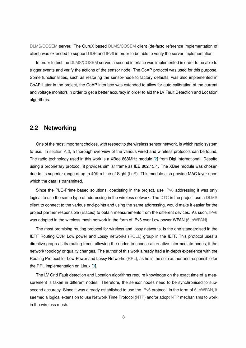
Figure 3.3 presents the stack of protocols to be used in the wireless mesh network. In the DTC,
there is a DLMS client running over UDP/IP and physically attached to the WMG through Ethernet. The
protocols used in the Radio-frequency (RF) network below the application layer are common Internet-of-
Things (IoT) standards, which are used in this type of networks, where power constrains and redundan-
cies are very important requirements. RPL provides routing in Low Power and Lossy Networks (LLNs),
enabling further stability through route optimisation and self-healing functionalities.
Figure 3.3: System Wireless Network Stack.
3.5.2 Availability and Synchronisation
To ensure a good operation of RF-Mesh, the WMG checks for connectivity issues by observing
activity from and to WMN, and by periodically issuing ping requests to a set of WMN. When possible
connectivity issues are detected, the WMG triggers RPL repair and schedule a check task to evaluate the
effect of RPL repair. If same issues are found, it’s issued an event notification about the unrecoverable
situation. The event notification might be system logger or a event notification by mail.
17
Since WMN require a time reference to timestamp sensor‘s readings, the WMG periodically sends
NTP reference to RF-Mesh. To allow the time synchronisation to be propagated in mesh depth, each
WMN must forward the time reference to current neighbours.
Although one might try to optimize this process by using a multicast mechanism to broadcast time
reference to all nodes, the system requires that time synchronisation use unicast mechanisms to each
neighbour. Since RPL protocol requires definition of nodes links quality evaluation function, joining a
RPL link weight evaluation function based on Expected Number of Transmissions (ETX) and the syn-
chronisation by unicast, will force the dynamic topology of RF-Mesh to stabilise quicker [7].
This operation scheme ensures that best links between nodes are selected as preferred RF-Mesh
routes.
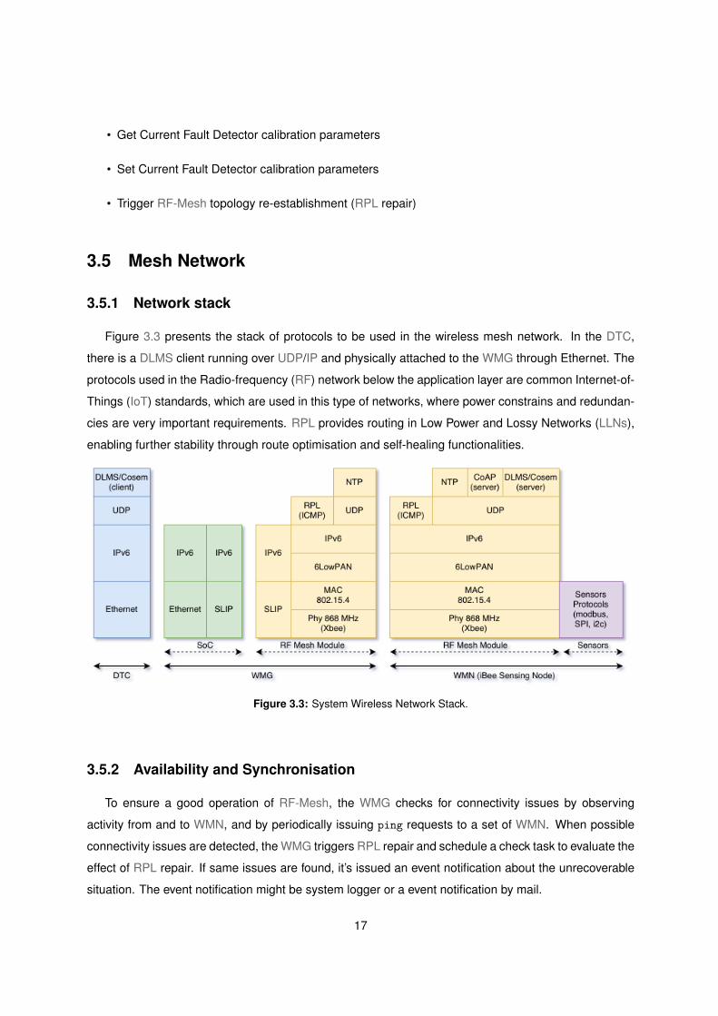
3.5.3 Pilot related network considerations
Since this system is part joint project, in order to allow debug of deployed sensors and to validate
software and hardware components before deployment, it has required special considerations on pilot
operation and test-bed environments. The Figure 3.4 show the connectivity between pilot and INOV
test-bed networks.
Figure 3.4: Network Stack between WMG and INOV networks.
3.6 Sensing Mechanisms
The WMN is responsible for providing DTC, any LV Grid measurements, whenever such request
arrive. It‘s noteworthy that on-demand readings and/or asynchronous readings are worthless if com-
pared or linked with any other readings. By this, it is very important to sense the LV Grid in discrete,
18

synchronised and time marked way.
The WMN is expected to gather all measurements by polling the several physical sensors at fixed,
but configurable, time interval. This time interval must be such that modulus of 60 by time interval is
zero. The WMN must also align the regular readings to each instant zero seconds of each minute, of
synchronised time reference from NTP.
The Figure 3.5 highlight the WMN physical sensors. There are sensors which must be requested
for readings and others that signal WMN for changes in the grid by interrupt. Since the hardware suffer
changes over time, there were versions that quickly signal by interrupt but others which performed better
in some aspect but failed to trigger MCU interrupt system.
Figure 3.5: iBee Block Diagram
To accomplish all types of sensors, hardware versions and measurements, the WMN simply polls
sensors in “on-demand” way, but using precise timer which triggers the readings on right time, likewise
for interrupt versions of sensors. The system then access to any sensor by common interface. The
mechanism of sensing continues with readings filtering and/or validation.
The WMN is also responsible for the detection of deviations of measurements to outbound limits
previously set. This is achieved by chaining the acquisition with basic predicate interface, provided in
the sensors common interface. These predicate interfaces provide simple way to detected the required
fault situations.
The sensing mechanisms of WMN merge the several nature of physical sensors, providing readings
19

validation, outbound value situations and asynchronous events.
The WMN will do synchronised measurements and be able to detect:
• Voltage outage in any phase by predicate function or interrupt sensor version
• Overload current in any phase by predicate function or interrupt sensor version
• Monitor battery limits in last-gasp situations
• Out of limits of voltage in any phase
• Out of limits of current in any phase
• Validate and/or filter faulty readings using hysteresis
• Case temperature conditions
3.7 Hardware Characteristics
3.7.1 Sensing Node
The Sensing Node developed at INOV is called iBee. The iBee nodes are designed around the
following requirements:
• low-power platform, with 30s last-gasp
• IPv6 (6LoWPAN) support
• RPL support
• 6 Digital I/O lines for the fault detector (fast detection of voltage and current faults)
• Serial port for modbus communication (and debug)
• 1 Digital I/O line for modbus communication
• Serial port for communication with the RF-module
Based on the above requirements, the iBee node is based on XBee communication module con-
trolled by an Integrated Circuit (IC) from the Atmel modified Harvard architecture 8-bit RISC single-chip
microcontroller (AVR) family, which is capable of running the Contiki OS. The later already has support
for IPv6 and RPL.
The block diagram of the iBee sensor node is given in Figure 3.5.
The central controller unit is based on the ATmega1284P AVR IC, which has 128kB Flash, 16kB
RAM and 4kB EEPROM. Furthermore it can runs with a frequency of up to 20MHz, although the iBee
20

uses a 8MHz clock to further reduced the power consumption. The AVR also has 2 hardware Universal
Asynchronous Receiver-Transmitter (UART), multiple Serial Peripheral Interface (SPI) ports, supports a
32kHz real-time clock and has a built-in watchdog timer.
The XBee communication module is connected to the central controller unit using a UART interface.
I/O lines are used to be able to reset the XBee when needed and an extra I/O line is used to be able to
remotely apply maintenance tasks on the main central unit.
The energy monitor unit is a standalone module, which measures voltages, currents and powers of
a 3-phase power system. The module communicates with the central controller unit using the modbus
protocol over a RS-485 serial interface, connected via a RS-485/UART converter to a separate UART of
the controller unit. This protocol is a master/slave bus and a header is added to the board for future ex-
tensions and as a debug interface. As the RS-485 is a master/slave system, where the central controller
unit is the master, the data is requested using polling. This module requires mains power and current
transformers to be able to monitor the power lines.
However, since fast detection of current and voltage faults are essential, a fault-detector module was
developed, which uses 6 I/O lines to communicate faults to the controller unit; three for voltages and
three for currents. These faults trigger an interrupt in the central controller unit, which can immediately
take the requires action.
When the iBee node looses the mains power (power outage) it still must be able to transmit this
failure to the DTC using the wireless mesh network. The aim is to provide communication for up to 30s
after a power failure. This is achieved using a 5F super-capacitor, which will take over the power supply
to the central controller unit and the XBee module.
The iBee sensor furthermore houses a digital thermometer IC and serial Electrically Erasable Pro-
grammable Read-Only Memory (EEPROM), both sharing the same SPI interface, but with different
chip-select I/O lines.
3.7.2 Wireless Mesh Gateway
The WMG was developed at INOV. The WMG was designed around the following requirements:
• IPv6-only gateway;
• RPL Root role;
• Monitoring, detection and repairing any issues related with mesh network;
• In pilot environment, provide network connectivity between INOV facilities over Internet and the
system for debugging purposes only. The WMG role does not requires Internet connectivity, on
the contrary, the WMG is meant to operate on secured and trusted network, only requiring a NTP
service within secured network.
21
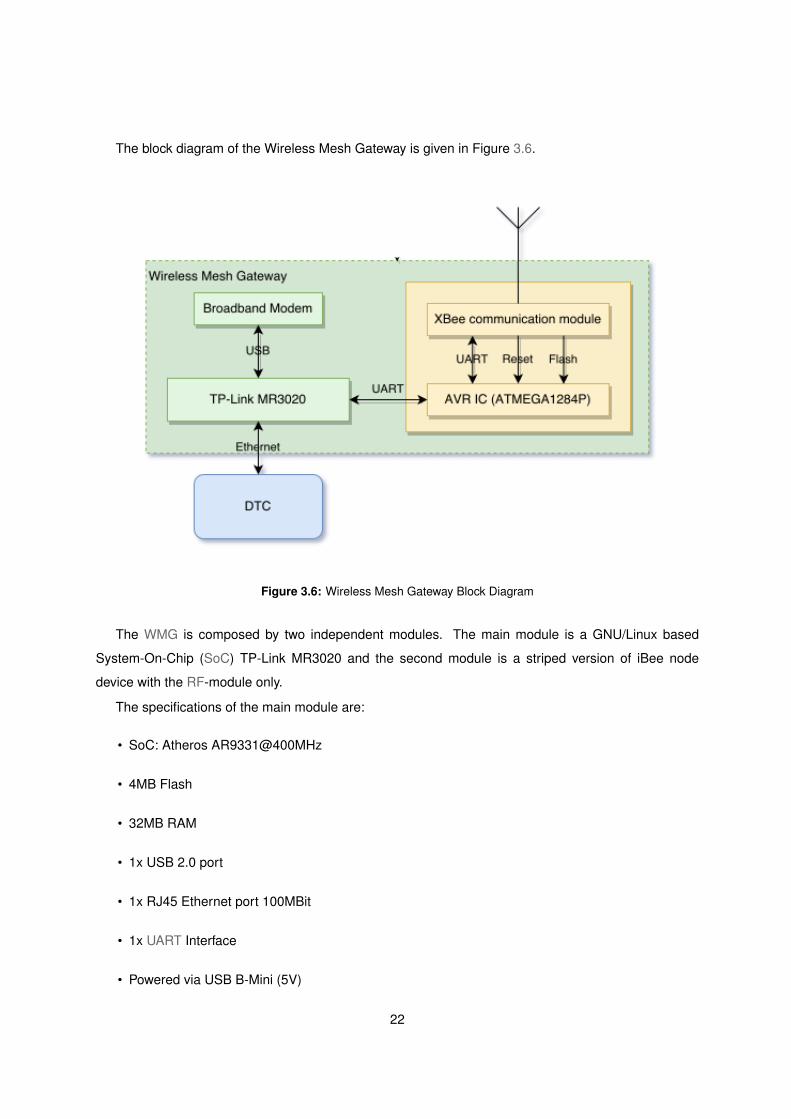
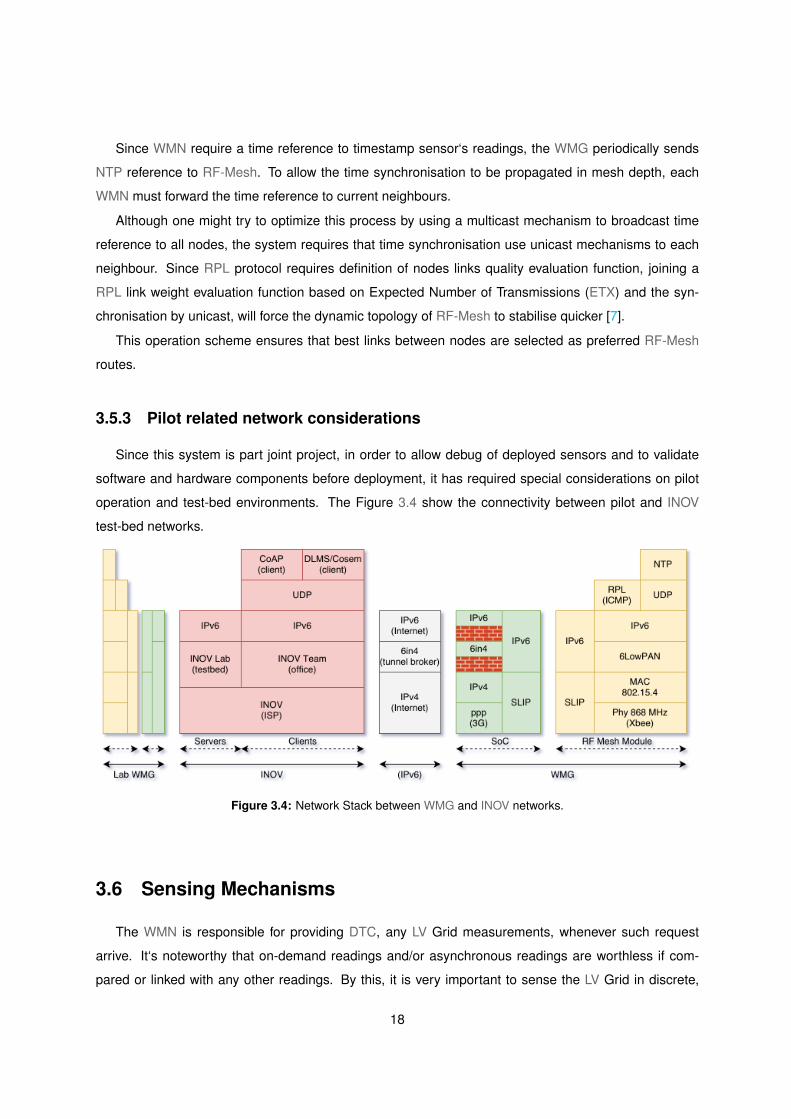
The block diagram of the Wireless Mesh Gateway is given in Figure 3.6.
Figure 3.6: Wireless Mesh Gateway Block Diagram
The WMG is composed by two independent modules. The main module is a GNU/Linux based
System-On-Chip (SoC) TP-Link MR3020 and the second module is a striped version of iBee node
device with the RF-module only.
The specifications of the main module are:
• SoC: Atheros AR9331@400MHz
• 4MB Flash
• 32MB RAM
• 1x USB 2.0 port
• 1x RJ45 Ethernet port 100MBit
• 1x UART Interface
• Powered via USB B-Mini (5V)
22

The main module features GNU/Linux based operation system, OpenWrt. OpenWrt is described as
a Linux distribution for embedded devices. Although ready to use builds of OpenWrt are available for
installation in many embedded devices, the WMG operates on a customised build of this distribution.
The OpenWrt system features a highly customisable build system, which allows to create a GNU/Linux
system with selective functionalities, such as, Linux base network stack, 3G/GPRS connectivity support,
basic command line tools, SSH server, HTTP server, firewall, web-page interface for configuration, etc.
Besides the basic GNU/Linux router functionalities and configuration tools, it was also included the WMG
related tools, features and mechanisms developed in this work, using the OpenWrt package system
and respective build system. One of the added features is related with communication with secondary
module using Serial Line Internet Protocol (SLIP) protocol. This link bridges all packets between RF
network and the DTC.
The specifications of the secondary module, striped version of iBee, are:
• AVR IC: ATmega1284P@8MHz
• 128kB Flash
• 16kB Random-Access Memory (RAM)
• 4kB EEPROM
• 2x UART Interfaces
• XBee RF-module
Likewise described in 3.7.1, the XBee communication module is connected to the AVR IC using a
UART interface. The second UART interface is linked to main module as IP bridge over SLIP protocol.
23

24

4System Implementation
This chapter describes the implementation of the various components of the system. The compo-
nents are divided into 5 parts:
Sensing modules: The drivers to connect the physical signals to sensor node
Networking modules Wireless transceiver driver and the various mechanisms developed to be able to
validate the reliability of the system
DLMS/COSEM server: A standards compliant server for DLMS/COSEM written from scratch.
CoAP Services: Standards compliant CoAP service (RFC 7252)
Wireless Flash: A mechanism to perform firmware updates without physical access to the nodes
Each node runs 2 services for interacting with the nodes. The first one is a standards compliant
DLMS/COSEM server written specifically with the aim for low computational resources (described in
Section 4.3 and the second one are the CoAP services (Section 4.4) that allows to interact with the
nodes more directly.
25

4.1 Sensing Modules
4.1.1 modbus Driver
Communication with the energy monitoring module takes place using the modbus protocol over
a RS-485 interface. The RS-485 protocol utilises a master/slave arrangement, where the monitoring
module is the slave and the central controller unit the master. The AVR does not have a native RS-485
interface, such that a RS-485 line-driver is used in half-duplex RS-485 mode, such that the direction of
transmission on the RS-485 transceiver by the central controller unit is controlled by an extra I/O line.
Given both WMN UART interfaces have dedicated functions, the RS-485 interface is also used for a
debug mode, which redirects any textual data over the RS-485 interface when LV sensor module is not
requesting data. Another advantage of using this interface is that RS-485 is a bus-protocol, allowing to
connect multiple slaves to the available interface.
4.1.2 LV Sensor
The LV sensor module is a Contiki Process responsible for obtaining the periodical measurements
from the energy monitoring modules, using the aforementioned modbus Driver. The process uses polling
to fetch measures from the available energy monitoring modules in short 30s intervals. For each energy
monitoring module, several measurements are requested, validated and processed.
The measurements requested are:
• Voltage
• Current
• Active Power
• Apparent Power
• Reactive Power
• Total Active Energy
The measurements above are requested for each channel available. The energy monitoring modules
may provide data for:
• one phase (L1)
• three phases (L1, L2, L3)
• four phases (L1, L2, L3 and Street Light)
26

The LV sensor module is also responsible for validating and process the measurements received. For
Voltage measurements and Current measurements, the process classify each value by level, based on
a set of thresholds pre-configured on the system. Thereafter, conditional actions may apply depending
on values levels.
Voltages are classified using 5 levels:
• Low Voltage
• Low Proximity Voltage
• Nominal
• High Proximity Voltage
• High Voltage
Nominal
Low ProximityVoltage
Low Voltage High VoltageHigh Proximity
Voltage
Figure 4.1: Voltages Thresholds
Currents only check for high current levels, since no minimal load (current draw) can be considered
as a fault. The currents classification uses the following 3 level:
• Nominal
• Low Overload
• High Overload
Nominal
High OverloadLow Overload
Figure 4.2: Currents Thresholds
Each boundary in level classification is checked using hysteresis.
By this, the LV sensor module can trigger an internal notification if a measurement level changes.
The trigger is performed depending on the alarm configuration. Each level can be pre-configured as
alarm enabled or alarm disabled.
27

All pre-configured settings on LV sensor module are persisted in EEPROM of WMN in order to survive
reboots and they are all editable by external control mechanisms. The LV sensor module settings are:
• Voltages Thresholds
• Current Thresholds
• Alarm Setting
• Hysteresis Parameters
The Last level classification status are also persisted.
4.1.3 Fault Detector Driver
The Fault Detector module is developed at INOV and is capable of detecting voltage faults and current
fault in 3 phases. When the voltage of a phase drops below a certain threshold, the module sets the
corresponding I/O line high, which causes an interrupt in the central controller unit. The current fault
detector follows a similar process, except triggers an interrupt when the current surpasses a certain limit
(short-circuit detection).
The Fault Detector Driver is a Contiki Process which is responsible for tracking I/O line levels. During
the development process and respective testing process it was used different hardware modules with
different signalling approaches. By this, the Fault Detector Driver also features a polling mode which
doesn’t make use of MCU interrupt system. In polling mode, the Fault Detector Driver keep track of
timings of I/O line levels changes. For each channel being tracked, a pre-configured time-out value is
used to classify I/O line levels changes as valid or noise.
The time-out values settings in Fault Detector Driver are also persisted in EEPROM of WMN and are
editable by external control mechanisms.
4.2 Networking Modules
4.2.1 XBee Communication Transceiver Driver
The XBee Communication Transceiver Driver is a Contiki Process which is responsible to translate
Contiki’s radio interface to Digi XBee API [2]. This driver is also responsible for conveying if a packet is
successfully delivered, whenever possible. This information is crucial for RPL mesh stability. The XBee
Communication Transceiver Driver allows the transmission power of XBee transceiver to be changed and
persisted. This setting is persisted in EEPROM of WMN and is editable by external control mechanisms.
28

4.2.2 TimeSync: NTP reference broadcast and RPL Parent Probing
The e-Balance project utilises data post-processing on the measured data to detect and locate errors,
and electricity fraud in the distribution network. This requires that the measured data is provided with a
sub-second accuracy in all nodes. The gateway uses a NTP-server to maintain its clock accurate and
periodically sends synchronization broadcast into the mesh.
Given limited resources in MCU, in order to get distribute a common time reference within mesh
network, a basic broadcast of authority rated time reference was used, directed downwards the mesh
tree, using each node’s preferred parent as the authority reference. The NTP client for Contiki was
already developed and has low overhead on firmware size [8].
Given the mesh availability requirements and the constrained use cases in power outages, it is critical
for mesh network nodes to recover quickly. The RPL stability convergence based on mesh network
traffic, delays considerably the reactive mechanisms which are required to guarantee mesh availability.
In order to allow each node to know the presence of neighbouring nodes, some periodic data exchange
between WMN is used, which triggers reactive RPL mechanisms [7].
In this case the TimeSync Module is developed as a Contiki Process responsible for probing all IPv6
neighbours for each WMN. Since RPL objective functions rely on the packet acknowledgement signal,
unicast transmissions are used. To make use of the periodic transmission between nodes, several data
is exchanged on probing packets.
Information included in TimeSync frames:
• authority level - analogous to NTP stratum [9]
• seconds - time reference timestamp
• collect period - time interval of debug appliances to be pushed to a data collector
• sink address - IPv6 address of debug data collector
4.2.3 3G Connection Checker
Given the deployment requirements of WMG and WMN, which are extremely restrictive in terms of
physical access to the equipments for safety reasons and, on the other hand, for security reasons of the
power grid, it was necessary to install broadband connectivity to WMG for remote debug, analysis and
testing purposes. In order to guarantee permanent connectivity using 3G USB modems and to be to
reset USB modems firmwares (due to some bugs in the USB models), it was required to reset USB bus
of WMG by disconnecting the USB opening circuit from the power supply.
The 3G Connection Checker module is responsible to periodically check direct connectivity of WMG
to INOV services and/or Google servers using Internet Control Message Protocol (ICMP). If no connec-
29

tivity is detected, the USB power is switched off for a few seconds to force the USB Modems to correctly
reset. This procedure guarantees that broadband connectivity is restored if service provider resets 3G
service.
4.2.4 pingstats
The pingstats module resides in WMG. This module is a small program that periodically issues
pings to a pre-configured list of WMN by IPv6 address to collect mesh network statistics data. For each
WMN is issued two pings with predefined sizes, respectively 20 and 60 bytes of ICMP payload, see
Section pingstats.
This module computes the follow data for each WMN:
• round-trip time (RTT)
• Bandwidth
• Depth in mesh tree
If some nodes do not reply to the periodic ping requests after a pre-configured number of tries, this
module send a RPL global repair to fix connectivity issues within mesh network. Unless the nodes are
without power, this is usually sufficient. The RPL global repair message has no negative impact on
correctly operating nodes in the same mesh.
4.2.5 meshstats
The meshstats module resides in WMG and is a program that make use of Linux nf conntrack to infer
WMN traffic with the DTC, simultaneous connections outbound/inbound mesh network and trace DLM-
S/COSEM request and responses sequences. This allows to trace, debug and improve mechanisms
and implementation of the DLMS/COSEM Server and DLMS/COSEM Clients.
4.2.6 Network Event Notifications
The Network Event Notification module resides in INOV network services. This module consists in
a variant of pingstats. The process is exactly the same as pingstats but with wider request periods.
In case of some node fail to reply ping requests for a pre-configure count of retries, this module sends
notification by mail to INOV team notifying the issue. An email is also send if unreachable nodes became
available.
30

4.3 DLMS/COSEM Server
DLMS is the most commonly used communication protocol in the area of (smart) metering across
the world [10]. DLMS is the Device Language Message specification, which defines the generalized
concepts for abstract modelling of communication entities. COSEM, the COmpanion Specification for
Energy Metering, is a set of rules for data exchange with energy meters . The DLMS/COSEM specifica-
tion is fully described in the DLMS UA coloured books, with the most interesting parts for the implemen-
tation in the Blue Book (COSEM meter object model and object identification system) [11, 12] and the
Green Book (application architecture, layers and transport protocols) [13]. As the service has to interact
with third-party DLMS/COSEM clients, it is vital that the service is standards compliant. DLMS uses
the XDR/ASN.1 [14,15] interface description language for defining data structures that can be serialized
and de-serialized in a standard, cross-platform way.
4.3.1 Requirements related choices
Recalling the requirements stated in previous chapters, the DLMS/COSEM server must provide a
service to get measurements from sensor, provide a service to set operation parameters, provide a
service to perform actions in the server and provide a service that send asynchronous notifications to
the client. These services must be served using a IPv6/UDP interface. It is also required that internal
state and internal configuration parameters to be persisted in external memory to be able to recover
from power outage situations. The server must restore it’s previous state on every system boot up, and
setup all configuration parameters in order to start to serve client requests.
The DLMS protocol defines that a server may support several clients, in particular to UDP wrapper,
several ports are available but only “Client Management Process” (0x0001) was defined. Any request re-
ceived with other destination is silently discarded. Since only one client (the DTC) was initially expected
to interact with DLMS/COSEM Server, only one Application Association (AA) is supported at same time.
Upon establishment of AA, client information is persisted. Upon graceful release of AA, client informa-
tion is cleared from persistent memory. Any successfully established AA is kept as active and valid even
if power outage and/or reboots take place. The current AA and client information might be updated upon
a successfully establishment of a new AA from the same or a different client.
4.3.2 Implemented Classes and OBIS Lists
As described in BlueBook [11,12], COSEM Interface classes (ICs) are defined by basic principles on
which ICs are build. This reference also documents how interface objects – instantiations of the ICs –
are used for communication purposes. The purpose of this specification is that it allows data collection
31

systems and metering equipment from different vendors, following these specifications, exchange and
interpret data seamless.
An object is a collection of attributes and methods, where attributes represent the characteristics
of an object. The value of an attribute may affect the behaviour of an object. The first attribute of
any object is the logical name. It is one part of the identification of the object. An object may offer a
number of methods to either examine or modify the values of the attributes. Objects that share common
characteristics are generalized as an interface class, identified with a class id. Within a specific ICs, the
common characteristics (attributes and methods) are described once for all objects. Instantiations of ICs
are called COSEM interface objects.
The BlueBook [11, 12] also defines how attributes and methods are referenced. There are two
different methods to reference attributes and methods of COSEM objects:
• Logical Names (LN referencing): In this case, the attributes and methods are referenced via the
identifier of the COSEM object instance to which they belong. The reference for an attribute is:
class id, value of the logical name attribute, attribute index.
• Short Names (SN referencing): This kind of referencing is intended for use in simple devices. In
this case, each attribute and method of a COSEM object is identified with a 13-bit integer.
Although it may seem that SN referencing is more ideal for the low resources node used in the
project, the third party client used by the partners in the project required that the DLMS/COSEM Server
uses the LN referencing method.
The class description notation used in BlueBook [11,12] describes the functionality and application of
the ICs. An overview of the ICs including the class name, the attributes, and the methods are presented
in tables 4.1 - 4.8. Each attribute and method is described in detail below.
The DLMS/COSEM Server implements the following ICs:
• IC 1: Data (See Table 4.1)Table 4.1: Data (class id: 1, version: 0)
Data 0..n class id = 1, version = 0
Attributes Data type Description
1. logical name octet-string Identifies the instantiation (COSEM object) of this IC.
2. value CHOICE Contains the data.
32

• IC 3: Register (See Table 4.2)Table 4.2: Register (class id: 3, version: 0)
Register 0..n class id = 3, version = 0
Attributes Data type Description
1. logical name octet-string Identifies the instantiation (COSEM object) of this IC.
2. value CHOICE Contains the current process or status value.
3. scaler unit scal unit type Provides information on the unit and the scaler of the value.
• IC 5: Demand Register (See Table 4.3)Table 4.3: Demand Register (class id: 5, version: 0)
Demand Register 0..n class id = 5, version = 0
Attributes Data type Description
1. logical name octet-string Identifies the instantiation (COSEM object) of this IC.
2. current average value CHOICE Provides the current value (running demand) of the energy accu-
mulated since start time, divided by number of periods*period.
3. last average value CHOICE Provides the value of the energy accumulated (over the last num-
ber of periods*period) divided by number of periods*period.
4. scaler unit scal unit type Provides information on the unit and the scaler of the value.
5. status CHOICE Provides “Demand register” specific status information.
6. capture time octet-string Provides the date and time when the last average value has
been calculated.
7. start time current octet-string Provides the date and time when the measurement of the cur-
rent average value has been started.
8. period double-long-unsigned Period is the interval between two successive updates of the
last average value.
9. number of periods long-unsigned The number of periods used to calculate the last average value.
33

• IC 7: Profile Generic (See Table 4.4)Table 4.4: Profile Generic (class id: 7, version: 1)
Profile Generic 0..n class id = 7, version = 1
Attributes Data type Description
1. logical name octet-string Identifies the instantiation (COSEM object) of this IC.
2. buffer compact-array or array Contains a sequence of entries.
3. capture objects array Specifies the list of capture objects that are assigned to the object
instance.
4. capture period double-long-unsigned Specifies the capturing period in seconds.
5. sort method enum Specifies the sort method.
6. sort object capture object definition If the profile is sorted, this attribute specifies the register or clock
that the ordering is based upon.
7. entries in use double-long-unsigned Counts the number of entries stored in the buffer.
8. profile entries double-long-unsigned Specifies how many entries shall be retained in the buffer.
Specific Methods m/o
1. reset(data) o Clears the buffer.
34

• IC 15: Association LN (See Table 4.5)Table 4.5: Association LN (class id: 15, version: 2)
Association LN 0..n class id = 15, version = 2
Attributes Data type Description
1. logical name octet-string Identifies the instantiation (COSEM object) of this IC.
2. object list object list type Contains the list of visible COSEM objects with their
class id, version, logical name and the access rights to
their attributes and methods within the given AA.
3. associated partners id associated partners type Contains the identifiers of the COSEM client and server
(logical device) APs within the physical devices hosting
these APs, which belong to the AA modelled by the “As-
sociation LN” object.
4. application context name application context name In the COSEM environment, it is intended that an appli-
cation context pre-exists and is referenced by its name
during the establishment of an AA.
5. xDLMS context info xDLMS context type Contains all the necessary information on the xDLMS
context for the given association.
6. authentication mechanism name mechanism name Contains the name of the authentication mechanism for
the association.
7. secret octet-string Contains the secret for the LLS or HLS authentication
process.
8. association status enum Indicates the current status of the association.
9. security setup reference octet-string References a “Security setup” object by its logical name.
10. user list array Contains the list of users allowed to use the AA managed
by the given instance of the “Association LN” class.
11. current user structure Holds the identifier of the current user.
35

• IC 67: Sensor Manager interface class (See Table 4.6)Table 4.6: Sensor Manager (class id: 67, version: 0)
Sensor Manager 0..n class id = 67, version = 0
Attributes Data type Description
1. logical name octet-string Identifies the instantiation (COSEM object) of this IC.
2. serial number octet-string Identifies the sensor.
3. metrological identification octet-string Describes metrologically relevant information of the sen-
sor.
4. output type enum Describes the physical output of the sensor.
5. adjustment method octet-string Describes the sensor adjustment method.
6. sealing method enum Type of seals applied to the sensor.
7. raw value CHOICE Physical value from the sensor.
8. scaler unit scal unit type The scaler and the unit of the raw value.
9. status CHOICE Status of last raw value captured (definition of status as
defined for “Extended register”).
10. capture time octet-string Provides a “Sensor manager” object specific date and
time information showing when the value of the attribute
raw value has been captured.
11. raw value thresholds array Provides the threshold values to which the raw value at-
tribute is compared.
12. raw value actions array Defines the scripts to be executed when the raw value
crosses the corresponding threshold.
13. processed value processed value definition References the attribute holding the processed value of
the raw data provided by the sensor.
14. processed value thresholds array Provides the threshold values to which the processed
value is compared.
15. processed value actions array Defines the scripts to be executed when the processed
value crosses the corresponding threshold.
Specific Methods m/o
1. reset(data) o This method resets the raw value to the default value.
The specification of IC 67 also required the implementation of function of the following ICs:
36

• IC 4: Extended Register (See Table 4.7)Table 4.7: Extended Register (class id: 4, version: 0)
Extended Register 0..n class id = 4, version = 0
Attributes Data type Description
1. logical name octet-string Identifies the instantiation (COSEM object) of this IC.
2. value CHOICE Contains the current process or status value.
3. scaler unit scal unit type Provides information on the unit and the scaler of the value.
4. status CHOICE Provides “Extended register” specific status information.
5. capture time octet-string Provides an “Extended register” specific date and time information showing when
the value of the attribute value has been captured.
37

• IC 21: Register Monitor (See Table 4.8)Table 4.8: Register Monitor (class id: 21, version: 0)
Register Monitor 0..n class id = 21, version = 0
Attributes Data type Description
1. logical name octet-string Identifies the instantiation (COSEM object) of this IC.
2. thresholds array Provides the threshold values to which the attribute of the referenced register is
compared.
3. monitored value value definition Defines which attribute of an object is to be monitored. Only values with simple
data types are allowed.
4. actions array Defines the scripts to be executed when the monitored attribute of the referenced
object crosses the corresponding threshold.
Each of the implemented COSEM objects are connected to one of the previously defined ICs. The
DLMS/COSEM Server provides the following COSEM objects instances with following ICs:
• IC 1: Data (version: 0)
– 0.0.96.7.0.255: Power Failure Monitor, last gasp count
– 0.128.97.97.0.255: Watchdog: failures counters
– 1.0.0.4.10.255: Ct Factor 3-phase meter
– 1.0.0.4.11.255: Ct Factor street-light meter
– 0.0.96.1.4.255: Device ID5
• IC 3: Register (version: 0)
– 0.0.67.128.9.255: Sensor Transmission Power
– 0.0.96.9.0.255: Enclosure Surface Temperature
– 0.0.96.12.5.255: RSSI
– 1.0.21.7.0.255: Instantaneous Active Power Phase 1
– 1.0.23.7.0.255: Instantaneous Reactive Power Phase 1
– 1.0.29.7.0.255: Instantaneous Apparent Power Phase 1
– 1.0.31.7.0.255: Instantaneous Current Phase 1
– 1.0.32.7.0.255: Instantaneous Voltage Phase 1
– 1.0.41.7.0.255: Instantaneous Active Power Phase 2
– 1.0.43.7.0.255: Instantaneous Reactive Power Phase 2
– 1.0.49.7.0.255: Instantaneous Apparent Power Phase 2
– 1.0.51.7.0.255: Instantaneous Current Phase 2
38

– 1.0.52.7.0.255: Instantaneous Voltage Phase 2
– 1.0.61.7.0.255: Instantaneous Active Power Phase 3
– 1.0.63.7.0.255: Instantaneous Reactive Power Phase 3
– 1.0.69.7.0.255: Instantaneous Apparent Power Phase 3
– 1.0.71.7.0.255: Instantaneous Current Phase 3
– 1.0.72.7.0.255: Instantaneous Voltage Phase 3
– 1.0.21.7.1.255: Instantaneous Active Power Street Light
– 1.0.23.7.1.255: Instantaneous Reactive Power Street Light
– 1.0.29.7.1.255: Instantaneous Apparent Power Street Light
– 1.0.31.7.1.255: Instantaneous Current Street Light
– 1.0.32.7.1.255: Instantaneous Voltage Street Light
– 1.0.1.8.0.255: Active energy import (+A)
• IC 5: Demand Register (version: 0)
– 1.0.32.5.0.255: Last Average Voltage L1
– 1.0.52.5.0.255: Last Average Voltage L2
– 1.0.72.5.0.255: Last Average Voltage L3
– 1.0.32.5.1.255: Last Average Street Light Voltage
– 1.0.31.5.1.255: Last Average Street Light Current
• IC 7: Profile Generic (version: 1)
– 0.0.97.98.1.255: Sensor Alarm Status
– 1.0.99.1.0.255: Load Profile
– 0.0.67.128.10.255: Instantaneous Voltage
– 0.0.67.128.11.255: Instantaneous Current
– 0.0.67.128.12.255: Instantaneous Active Power
– 0.0.67.128.13.255: Instantaneous Reactive Power
– 0.0.67.128.14.255: Instantaneous Apparent Power
• IC 67: Sensor Manager interface class (version: 0)
– 0.0.67.128.0.255: Current Alarm Phase 1
39

– 0.0.67.128.1.255: Current Alarm Phase 2
– 0.0.67.128.2.255: Current Alarm Phase 3
– 0.0.67.128.3.255: Voltage Alarm Phase 1
– 0.0.67.128.4.255: Voltage Alarm Phase 2
– 0.0.67.128.5.255: Voltage Alarm Phase 3
– 0.0.67.128.6.255: Temperature Alarm
– 0.0.67.128.7.255: Street Light Current Alarm
– 0.0.67.128.8.255: Street Light Voltage Alarm
• IC 15: Association LN (version: 2)
– 0.0.40.0.0.255: List of objects
4.3.3 Considerations related to Server Program Code
The design and implementation of the DLMS/COSEM server was surrounded by several software
and hardware limitations. Since the DLMS/COSEM specifications are extremely extend, only the mini-
mum required functionalities were implemented. The implementation should use program code instead
of RAM memory, given the low memory resources. At the same time, program code should be optimized
to allow a complete implementation of the services and provide acquisition of all measurements.
In order to keep track of available RAM memory during development and implementation of software,
a stack buffer overflow protection scheme was implemented. The protection scheme implemented was
a stack canary based scheme. Although stack canary schemes are commonly used for malicious code
detection, the adopted scheme was used to track unused RAM space. This was achieved by spraying all
free RAM with a well-known value on boot, and during operation, by periodical counting the unused RAM
addresses (unchanged well-known value). The untouched RAM count is obtain via the debug interface.
To minimize the usage of RAM, it was adopted a static method to encode the server behaviour.
Instead the use of iteration of RAM with the objects list, the list was declared and completely encoded
using C pre-compiler macros and C enumerations, in such way that objects could be referenced using
a simple integer instead the respective interface class and OBIS (which would take 8 bytes, otherwise).
Making use of C language switch control keyword, all objects were encoded flatten in program code.
This way, the server implementation also spare several bytes on heap during functions invocations
and eventual recursions, and also gets performance given direct jump of switch case control and the
absence of string lookups. The down side of this approach is that objects references pre-defined by C
pre-compiler could change between versions. New re-configuration is required if objects list change.
40

1 #ifndef DLMS_OBJECTS_H_2 #define DLMS_OBJECTS_H_34 #include <dlms-types.h>56 #define OBIS_OBJECTS \7 /* Sensor Transmission Power */ \8 OBIS(3,0,0,67,128,9,255,AT_DOUBLE_LONG) \9 /* Street Light Current Alarm */ \
10 OBIS(67,0,0,67,128,7,255,AT_LONG_UNSIGNED) \11 /* Street Light Voltage Alarm */ \12 OBIS(67,0,0,67,128,8,255,AT_LONG_UNSIGNED) \13 \14 /* Device ID5 */ \15 OBIS(1,0,0,96,1,4,255,AT_OCTET_STRING) \16 /* Load Profile */ \17 OBIS(7,1,0,99,1,0,255,AT_ARRAY) \18 \19 /* Power Failure Monitor, last gasp */ \20 OBIS(1,0,0,96,7,0,255,AT_DOUBLE_LONG) \21 /* Sensor Alarm Status */ \22 OBIS(7,0,0,97,98,1,255,AT_ARRAY) \23 \24 /* Last Average Street Light Voltage */ \25 OBIS(5,1,0,32,5,1,255,AT_LONG_UNSIGNED) \26 /* Last Average Street Light Current */ \27 OBIS(5,1,0,31,5,1,255,AT_LONG_UNSIGNED) \28 \29 /* List of objects */ \30 OBIS(15,0,0,40,0,0,255,AT_ARRAY) \31 /* Watchdog: conditional failures counters */ \32 OBIS(1,0,128,97,97,0,255,AT_OCTET_STRING)3334 #define OBIS(ic,a,b,c,d,e,f,g) OBISCODE_##a##_##b##_##c##_##d##_##e##_##f,35 enum obis_ids 36 OBIS_CODE_DUMMY = -1,37 OBIS_OBJECTS38 OBISCODE_LAST39 ;40 #undef OBIS4142 extern const __attribute__((__progmem__)) dlms_objects_t obis_codes[];4344 #endif /* DLMS_OBJECTS_H_ */
Listing 4.1: Example of COSEM objects list definition
1 #include <dlms-objects.h>23 #define OBIS(ic,a,b,c,d,e,f,g) ic,a,b,c,d,e,f,4 const __attribute__((__progmem__)) dlms_objects_t obis_codes[] = 5 OBIS_OBJECTS6 ;7 #undef OBIS
Listing 4.2: Example of COSEM objects list instantiation
1 data_access_result_t get_ic1(uint8_t *resp_buf, uint16_t *response_len, int obiscode, uint8_tattr_id) →
2 if (attr_id > 2) 3 return DATA_ACCESS_OBJECT_CLASS_INCONSISTENT;4 5 uint8_t *pData = resp_buf;6 uint32_t value = 0;7 uint16_t max_len = DLMS_MSG_MAX_SIZE - *response_len;8 char id5str[14]; UNUSED(id5str);9 linkaddr_t eui64; UNUSED(eui64);
1011 #if PLATFORM_HAS_WATCHDOGCONDITIONAL12 uint8_t wdcnt[8];13 int cnts;14 int i;15 uint8_t *pStruct;16 #endif1718 PRINTF("> get_ic1: len: %u obiscode: %d (%d)\n",*response_len,obiscode,attr_id);1920 switch (obiscode)
41

21 #if PLATFORM_HAS_WATCHDOGCONDITIONAL22 case OBISCODE_0_128_97_97_0_255:23 cnts = watchdog_get_failed_conditions(wdcnt, 8);2425 pStruct = create_seq(&pData, max_len, NULL, ATTR_TYPE(AT_STRUCTURE));26 for(i=0;i<cnts;i++) 27 push_unsigned(&pData, max_len, pStruct, UNSIGNED(wdcnt[i]));28 2930 break;31 #endif32 #if PLATFORM_HAS_IBEE33 case OBISCODE_0_0_96_1_4_255:34 ibee_get_eui64(eui64.u8);35 sprintf(id5str,"INO%02x%02x%02x%02x%02x",36 eui64.u8[3], eui64.u8[4], eui64.u8[5], eui64.u8[6], eui64.u8[7]);37 push_octet_str(&pData, max_len, NULL, OCTET_STR(id5str, sizeof(id5str) - 1));38 break;39 #endif /* PLATFORM_HAS_IBEE */40 case OBISCODE_0_0_96_7_0_255:41 value = power_failure_count;42 push_double_long_unsigned(&pData, max_len, NULL, &value);43 break;44 case OBISCODE_1_0_0_4_10_255:45 #if PLATFORM_HAS_IME46 value = get_kta_meter(1);47 push_double_long_unsigned(&pData, max_len, NULL, &value);48 #else49 return DATA_ACCESS_READ_WRITE_DENIED;50 #endif51 break;52 #ifdef ENABLE_STREET_LIGHT53 case OBISCODE_1_0_0_4_11_255:54 #if PLATFORM_HAS_IME55 value = get_kta_meter(2);56 push_double_long_unsigned(&pData, max_len, NULL, &value);57 #else58 return DATA_ACCESS_READ_WRITE_DENIED;59 #endif60 break;61 #endif62 63 *response_len += (pData - resp_buf); // Total response length64 PRINTF("< get_ic1: len: %u obiscode: %d (%d)\n",*response_len,obiscode,attr_id);65 return DATA_ACCESS_SUCCESS;66
Listing 4.3: Example of IC1 get attribute function
Given the several configurations and features available within the several variations of hardware of INOV
sensor, the configuration of build process and compilation of firmware activates or disables program
code when not required by hardware variations. The complete definition of objects list depending on
sensor is available in Appendix B, listing C.2.
Table 4.9: Firmware sizes
Build version Program (max. 126 kBytes) Data (max. 16 kBytes) DLMS Objects(.text + .data) (.data + .bss + .noinit)
3 phases firmware 122938 bytes (95.3 %) 14728 bytes (89.9 %) 413 phases + street light firmware 125536 bytes (97.3 %) 15222 bytes (92.9 %) 513 phases without modbus interface 120544 bytes (93.4 %) 14701 bytes (89.7 %) 41test firmware with dummy sensor 113720 bytes (88.1 %) 14657 bytes (89.5 %) 41
Although Program Code available in MCU is 128 kBytes, the sensor requires 2048 bytes to be reserved
to boot-loader. Thus the firmware code must not exceed 98.44% (129028 of 131072 bytes) of MCU
Program Code space.
42

4.4 CoAP Services
• Get Firmware Release Version and build dateTable 4.10: Get Firmware Release Version and build date CoAP Service
Title Get Firmware Release Version and build date.
URL /root
Method GET
Success Response Example:
Code: 205 CONTENT
Content: “Contiki-915fb1988 (Feb 14 2017 11:30:14)”
Error Response Not applicable. Success response is guaranteed.
Sample Call $ coap-client coap://dummy0.pt000.mbt.sgwg.inov.pt/root
Contiki-915fb1988 (Jan 5 2017 11:05:59)
• Reset/Erase persistent data from sensor modules (settings, watchdog counters)Table 4.11: Reset/Erase persistent data from sensor modules CoAP Service
Title Reset/Erase persistent data from sensor modules (settings, watchdog counters).
URL /root?format=:storage&please=:confirm flag
Method POST
URL Params Required:
storage=[“settings” | “wdtcnts”]
confirm flag=“yes”
example: format=settings&please=yes
Success Response Example:
Code: 205 CONTENT
Content: “Contiki-915fb1988 (Feb 14 2017 11:30:14)”
Error Response Example:
Code: 405 METHOD NOT ALLOWED
Reason: The sensor has no storage support.
OR
Code: 406 NOT ACCEPTABLE
Reason: Confirm flag provided with wrong value.
OR
Code: 400 BAD REQUEST
Reason: Storage value provided is not valid or not supported by the sensor.
Sample Call $ coap-client -m post coap://pl0.pt000.mbt.sgwg.inov.pt/root?format=settings&please=yes
Contiki-915fb1988 (Jan 5 2017 11:05:59)
43

• Force Non-graceful Reboot of the sensorTable 4.12: Force Non-graceful Reboot of the sensor CoAP Service
Title Force Non-graceful Reboot of the sensor.
URL /reboot
Method POST | PUT
Success Response Example:
Code: 205 CONTENT
Content: “initiating reboot”
Error Response Not applicable. Success response is guaranteed.
Sample Call $ coap-client -m post coap://dummy0.pt000.mbt.sgwg.inov.pt/reboot
initiating reboot
• Get radio module statisticsTable 4.13: Get Radio module statistics CoAP Service
Title Get radio module statistics: power level, duty-cycle and temperature.
URL /tx
Method GET
Success Response Example:
Code: 205 CONTENT
Content: “pl: 2 dc: 5 t: 48”
Error Response Not applicable. Success response is guaranteed.
Sample Call $ coap-client coap://dummy0.pt000.mbt.sgwg.inov.pt/tx
pl:2 dc:5 t:48
• Set radio module transmit powerTable 4.14: Set radio module transmit power CoAP Service
Title Set radio module transmit power.
URL /tx?pl=:power level
Method POST
URL Params Required:
power level=[integer 0..4]
example: pl=2
Success Response Example:
Code: 205 CONTENT
Error Response Example:
Code: 400 BAD REQUEST
Reason: Provided power level out of boundaries.
OR
Code: 500 INTERNAL SERVER ERROR
Reason: Some error occur applying power-level changes.
Sample Call $ coap-client -m post coap://root.pt000.mbt.sgwg.inov.pt/tx?pl=2
44

• Trigger DLMS/COSEM Event Notification service indication on DLMS Server. Destination will be
last client that performed a successful application association.Table 4.15: Trigger DLMS/COSEM Event Notification CoAP Service
Title Trigger DLMS/COSEM Event Notification service indication on DLMS Server.
URL /dlms ev?s=:class obis attr
Method POST
URL Params Required:
class obis attr=IC.A.B.C.D.E.F.attr where IC is class, A..F is OBIS and attr is attribute index as described
in BlueBook [11, 12] sections Class description notation, Relation to OBIS and COSEM Object Iden-
tification System (OBIS).
example: s=7.0.0.97.98.1.255.2
Success Response Example:
Code: 205 CONTENT
Content: “Done”
Error Response Not applicable. Success response is guaranteed.
Sample Call $ coap-client -m post coap://dummy5.pt000.mbt.sgwg.inov.pt/dlms ev?s=7.0.0.97.98.1.255.2
Done
45

• Get LV Sensor calibration parametersTable 4.16: Get LV Sensor calibration parameters CoAP Service
Title Get LV Sensor calibration parameters.
URL /lvcal?v=:get voltages factors&i=:get currents factors&e=:get energy factor
Method GET
URL Params Optional:
get voltages factors=[alphanumeric]
example: v=1
get currents factors=[alphanumeric]
example: i=1
get energy factor=[alphanumeric]
example: e=1
Success Response Example:
Code: 205 CONTENT
Content:
“1: 1.000000
2: 1.000000
3: 1.000000
4: 1.000000”
Error Response One of optional parameters is expected. Success response is guaranteed. If none of optional
parameters is provided and/or energy factor requested but unsupported, the following response
is returned:
Code: 205 CONTENT
Content: “select v=1 or i=1”
Sample Call $ coap-client coap://dummy1.pt000.mbt.sgwg.inov.pt/lvcal?v=1
1: 0.999102
2: 0.999551
3: 1.001351
4: 1.000000
46

• Set LV Sensor calibration parametersTable 4.17: Set LV Sensor calibration parameters CoAP Service
Title Set LV Sensor calibration parameters.
URL /lvcal?p=:phase&v=:voltage&vf=:voltage factor&i=:current&if=:current factor
Method POST
URL Params Required:
phase=[integer]
example: p=1
Optional:
voltage=[integer]
example: v=2310
voltage factor=[integer]
example: vf=1001
current=[integer]
example: i=50
current factor=[integer]
example: if=1000
Success Response Example:
Code: 205 CONTENT
Content: “Updated phase 1”
Error Response Example:
Code: 400 BAD REQUEST
Reason: Wrong parameters provided and/or missing parameters.
Sample Call $ coap-client -m post coap://dummy0.pt000.mbt.sgwg.inov.pt/lvcal?p=1&v=2300
Updated phase 1
47

• Get Current Fault Detector calibration parametersTable 4.18: Get Current Fault Detector calibration parameters CoAP Service
Title Get Current Fault Detector calibration parameters.
URL /lvf?v=:get values
Method GET
URL Params Optional:
get values=[alphanumeric]
example: v=1
Success Response Example:
Code: 205 CONTENT
Content:
“t:2450
h:4
d:996
m:E4”
OR
Code: 205 CONTENT
Content:
“0:970
1:183
2:275”
Error Response Not applicable. Success response is guaranteed.
Sample Call $ coap-client coap://dummy1.pt000.mbt.sgwg.inov.pt/lvf
t:2450
h:4
d:996
m:E4
48
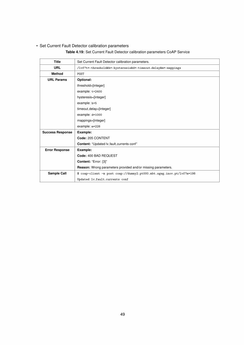
• Set Current Fault Detector calibration parametersTable 4.19: Set Current Fault Detector calibration parameters CoAP Service
Title Set Current Fault Detector calibration parameters.
URL /lvf?t=:threshold&h=:hysteresis&d=:timeout delay&m=:mappings
Method POST
URL Params Optional:
threshold=[integer]
example: t=2400
hysteresis=[integer]
example: h=5
timeout delay=[integer]
example: d=1000
mappings=[integer]
example: m=228
Success Response Example:
Code: 205 CONTENT
Content: “Updated lv fault currents conf”
Error Response Example:
Code: 400 BAD REQUEST
Content: “Error: [3]”
Reason: Wrong parameters provided and/or missing parameters.
Sample Call $ coap-client -m post coap://dummy2.pt000.mbt.sgwg.inov.pt/lvf?m=198
Updated lv fault currents conf
49

• Trigger RF-Mesh topology re-establishment (RPL repair)
Table 4.20: Trigger RF-Mesh topology re-establishment (RPL repair) CoAP Service
Title Trigger RF-Mesh topology re-establishment (RPL repair).
URL /repair
Method POST
Success Response Example:
Code: 205 CONTENT
Content: “calling repair”
Error Response Example:
Code: 404 NOT FOUND
Reason: This service is only available in gateway nodes.
Sample Call $ coap-client -m post coap://root.pt000.mbt.sgwg.inov.pt/repair
calling repair
4.5 Wireless Flash
The iBee sensor is to installed in places with difficult physical access, such as high up in a utility pole
of the low-voltage energy network, or inside a distribution cabinet. Therefore it must be possible to
update the firmware via the wireless interface, but without the need of a working network. This allows
the sensor to be updated, even if it has become unresponsive or has not joined a network. This requires
the wireless module to be able to reset the controller unit and put it in firmware uploading mode, which
is depicted in the Figure 4.3.
The XBee Transceiver Module operates independent from the main iBee MCU. Therefore, even if the
main iBee MCU locks up or ends up in a boot-loop, it is still possible to take over control via the Wireless
Flash interface. The remote Xbee Transceiver Module sets a flash-signal and subsequently resets the
iBee MCU. Upon every boot, the MCU boot-loader checks if the flash-signal is set and changes the
internal boot-loader to receive the firmware update via the XBee Transceiver Module. The remote Xbee
Transceiver resets the flash-signal and then reboots the iBee MCU if the process has ended.
50

Figure 4.3: Wireless Flash Sequence Diagram
51

52
5System Validation
The developed system from this work is validated in three parts: sensor components, the sensor as a
whole and the system as being operated in the demonstrator.
5.1 Hardware Appliance Robustness and Reliability Evaluation
This section validates the various components of the developed wireless sensor.
5.1.1 Reliability: graceful and non-graceful reboot tests
To test the RPL recovery and correct boot after non-graceful reboots a test-bed was prepared to stress
the nodes’ hardware. An Arduino is used to control a relay, which switched the power to sensors on
and off. The time to all sensors to respond to pings, which can only occur after the sensor has correctly
booted and joined the mesh network, was measured. The sensors were rebooted 1000 times and
successfully recovered every time. The script used to monitor this process is given in Appendix C.1.
A test-bed was prepared with a root node and three leaf nodes. The script waits for the root to boot
53

and reply to pings. When the RPL mesh is ready, the script proceeds with pings to leafs nodes. The
results for the root are given in Figure 5.1 and for the leaf-nodes 1, 2 and 3 in Figures 5.2, 5.3 and 5.4,
respectively.
200 400 600 800sample
10
20
30
40
50
total(s)
Figure 5.1: Test reboot: Root Node (Sensor 5c60)
200 400 600 800sample
10
20
30
40
50
60
70
total(s)
Figure 5.2: Test reboot: Leaf #1 (Sensor c99d)
200 400 600 800sample
50
100
150
200
total(s)
Figure 5.3: Test reboot: Leaf #2 (Sensor c95a)
Table 5.1: Reboot Test Time Results
Sensor Average Std Deviation
Root Node (Sensor 5c60) 20.521s 4.838
Leaf #1 (Sensor c99d) 21.493s 5.728
Leaf #2 (Sensor c95a) 22.276s 9.880
Leaf #3 (Sensor c999) 23.095s 7.130
54

200 400 600 800sample
25
50
75
100
125
total(s)
Figure 5.4: Test reboot: Leaf #3 (Sensor c999)
The normalization delay of the RPL root is given in Table 5.1. The delay until the root replies to pings
is justified by the bootstrap time of the root node, which includes the setup of the SLIP interface, ini-
tialization of the IPv6 prefix, update of the system time and the RPL initialization. As soon as the root
node finishes the bootstrapping, leaf nodes can join the RPL mesh and all nodes start replying to pings
consistently along reboots.
5.1.2 Diagnostics Self-test and Calibration
Diagnostic information from the sensors can be obtained with the RS485 interface, four leds of the
sensor and a single button. In order to simplify the deployment process and implement a quality check
for the sensors, a special firmware mode was developed that checks all internal functionalities of the
sensors and automatically calibrates internal sensor with a trusted external reference.
A test sequence and check-list is used to check all sensors to aid in the detecting of any errors or faulty
sensors before they are delivered to partners and before they are deployed in the demonstrator site.
The test and calibration mode requires the use of the RS485 interface, shared with a laptop used for
debugging the internal sensors and external reference sensor. The reference sensor uses the modbus
protocol, which makes it possible to connect several devices to the same bus and get debug output. The
test and calibration mode is divided into several test stages. The operator uses the debug button to enter
and forward each stage. The check-list specifies the operator inputs and which outputs are expected for
each stage and is given in Table 5.2.
5.1.3 Appliance power failure mechanisms tests
As described in the system requirements, the sensor must be able to relay and/or transmit any failures
or power outage situations for at least 30s after the outage. This time-window is referred to as last-gasp
time.
During the design, development and testing stages the last-gasp time was daily observed when sensors
55

Table 5.2: Self Test and Calibration Check-list
Stage Description External Action Expected Results1 Leds None Observable 1s pace leds sequence:
1. all OFF2. led 1 ON3. leds 1 and 2 ON4. leds 1,2 and 3 ON5. all ON6. leds 2,3 and 4 ON7. leds 3 and 4 ON8. led 4 ON9. sequence restart
2.1 Voltage FaultDetection L1
1. Simulate non fault L12. Simulate fault L1
Observable:1. Led 1 turns ON2. Led 1 turns OFF
2.2 Voltage FaultDetection L2
1. Simulate non fault L22. Simulate fault L2
Observable:1. Led 2 turns ON2. Led 2 turns OFF
2.3 Voltage FaultDetection L3
1. Simulate non fault L32. Simulate fault L3
Observable:1. Led 3 turns ON2. Led 3 turns OFF
3.1 Current FaultDetection L1
1. Simulate non overload L12. Simulate overload L1
Observable:1. Led 1 turns ON2. Led 1 turns OFF
3.2 Current FaultDetection L2
1. Simulate non overload L22. Simulate overload L2
Observable:1. Led 2 turns ON2. Led 2 turns OFF
3.3 Current FaultDetection L3
1. Simulate non overload L32. Simulate overload L3
Observable:1. Led 3 turns ON2. Led 3 turns OFF
4 Xbee None Observable messages output sequence:1. Init: “Xbee initialized OK”2. MAC: “EUI64: XX:XX:XX:XX:XX:XX:XX:XX OK”3. Temp: “Temp: dd OK”4. VCC: “VCCin: ddd OK”5. DutyCycle: “Duty: dd OK”6. Sequence continues from 2.
5 IME None Observable messages output sequence:1.“L1 V: ddd I: ddd”“L2: V: ddd I: ddd”“L3: V: ddd I: ddd”“OK”2.“L1 Act: ddd React: ddd”“L2: Act: ddd React: ddd”“L3: Act: ddd React: ddd”“OK”
6 Temperature None Observable messages output,such as 15.000 <ddddd <30.000:“Temperature: ddddd”
where disconnected from the grid or when the power failure mechanisms where activated. The time
observed was always larger than 2 minutes, after which the sensor could not guarantee a minimum of
3 volts to operate the Xbee communication module. When this voltage boundary is crossed, the sensor
can no longer communicate and all peripherals are switched off before entering a sleep mode.
The sleep mode allows the sensor to maintain all mesh data in memory, optimizing the recover process
when power is restored as it does not have to reconfigure the network. Most of the times, the network
56
has not changes as all sensors in the project are stationary.
The sleep mode is maintained until the MCU consumed all energy from super-capacitors or its power
is restored. It was verified that the sensor shuts down completely when the voltage is lower than 1.8V.
During the sleep mode, a distinct led composition is activated every 5s indicating the super capacitor
status. The sensor can be kept in sleep mode for over 4 hours.
As the observed last-gasp time was very much superior to the 30s requirement, no statistical testing
were deemed necessary.
5.1.4 Gateway WAN Connectivity tests
As some of the USB modems do not correctly reset, a band-aid solution had to be implemented. The
correct reset of the USB modems is guaranteed by switching off the power to the USB bus. This guar-
antees the correct recovery of the 3G Connection and respective USB dongle. The USB bus resets
are logged in a file on the gateway, which is located in RAM. This means that this information is not
persistent over reboots of the gateway. At the time of writing the log-file has the following occurrences:
Tue Oct 10 13:30:40 WEST 2017
Tue Oct 10 13:32:43 WEST 2017
Wed Oct 11 11:02:14 WEST 2017
Since the 3G ISP provider does not provide IPv6 connectivity, a 6in4 tunnel was setup to a Tunnel Broker.
The gateway firmware adopted provided a service to update the dynamically assigned IPv4 address of
the 3G dongle, which is needed to update the 6in4 tunnel endpoints, see Figure 5.5.
5.2 System Performance and Availability Evaluation
In contrast to the previous section, this section looks into the tests, which where performed to quantify
the performance of the system.
The radio modules of the e-Balance Mesh network devices have a throughput of 24kb/s, according to the
manufacturers data-sheet. However, European law limits the duty-cycle of equipment operating in the
868MHz bands to 10%, effectively reducing the throughput to 2.4kb/s. This report estimates the latency
and bandwidth of the mesh network, both in a laboratory setup at INOV and in the field and compares
them to the values from the manufacturer.
57
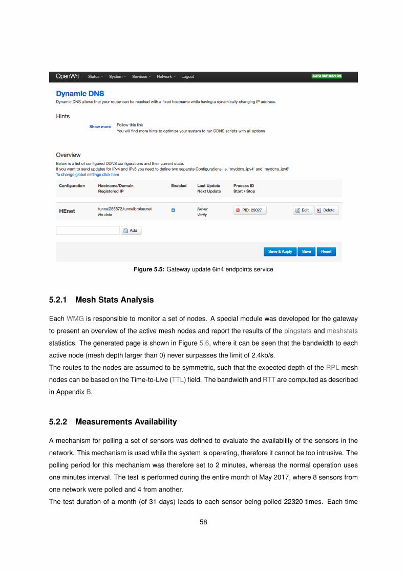
Figure 5.5: Gateway update 6in4 endpoints service
5.2.1 Mesh Stats Analysis
Each WMG is responsible to monitor a set of nodes. A special module was developed for the gateway
to present an overview of the active mesh nodes and report the results of the pingstats and meshstats
statistics. The generated page is shown in Figure 5.6, where it can be seen that the bandwidth to each
active node (mesh depth larger than 0) never surpasses the limit of 2.4kb/s.
The routes to the nodes are assumed to be symmetric, such that the expected depth of the RPL mesh
nodes can be based on the Time-to-Live (TTL) field. The bandwidth and RTT are computed as described
in Appendix B.
5.2.2 Measurements Availability
A mechanism for polling a set of sensors was defined to evaluate the availability of the sensors in the
network. This mechanism is used while the system is operating, therefore it cannot be too intrusive. The
polling period for this mechanism was therefore set to 2 minutes, whereas the normal operation uses
one minutes interval. The test is performed during the entire month of May 2017, where 8 sensors from
one network were polled and 4 from another.
The test duration of a month (of 31 days) leads to each sensor being polled 22320 times. Each time
58

Figure 5.6: Gateway Mesh Nodes: Overview web page
a node is polled, a IC7 with load profile and IC3 with Total Positive Active Energy are requested. An
attempt is only recorded as successful, when both request give the proper response. The results for the
test of May 2017 are given in Figure 5.7.
2017-05-04 2017-05-11 2017-05-18 2017-05-25Date
0
2,5
5
7,5
10
SuccessfulSamplesCount
Figure 5.7: Measurements Availability May 2017
The results of this test also allow to obtain the success ratio within the expected sample count, as shown
in Table 5.3.
The Table 5.3 shows that 21724 times out of 22320 all 12 sensors responded correctly, 434 times one
sensor did not respond and in 42 cases none of the sensors responds correctly. This gives an availability
59

Table 5.3: Measurements Availability Results
Sensors Count Samples Count Overall ratio0 42 0.188%1 2 0.009%3 1 0.004%4 1 0.004%6 4 0.017%7 5 0.022%8 32 0.143%9 19 0.085%10 43 0.192%11 434 1.944%12 21724 97.329%
for the entire network of 97.33% and a single sensor availability, the probability that a sensor responds
successfully to the 2 requests of 99.75%.
5.3 Demonstrator Operation System Evaluation
The demonstrator is installed in the EDP Distribuicao electrical distribution grid in the municipality of
Batalha in Portugal [16]. The e-balance project defined an extensive set of use cases, which reflect the
capabilities of the e-balance platform mechanisms for:
i neighbourhood monitoring in the Low-Voltage (LV) distribution grid;
ii smart MV distribution grid;
iii energy balancing;
iv customer data handling and customer interaction.
The sensors described in this thesis are part of the 2nd use case dealing with the LV distribution grid.
The e-balance demonstrator for the LV segment of the grid focuses on creating the means to enable a
Distribution System Operator to:
• Measure in a near real-time approach, consumption power flows;
• Measure in a near real-time approach, production power flows from distributed energy resources;
• Detect and locate commercial losses (frauds);
• Locate and detect faults within the LV grid;
• Calculate energy distribution losses;
• Calculate quality of service performance indicators with more accuracy.
60

Overall, this set of objectives will lead to a significant improvement in the LV grid service quality and
resilience.
The sensors developed in this work are involved in the measuring of Neighbourhood power flows, which
has as its main goal to get a macro view of power flows along the LV feeders. The sensors are also used
for LV fault detection and location, which firstly has to detect faults in the LV grid and secondly determine
the fault location. Some of the sensors are equipped with a public lighting monitor, which can be used
to detect and locate public lighting faults and blown light bulbs.
The sensors can send an event notification when detecting various voltage thresholds, which is used
to prevent voltage limit violations based on voltage measurements of the LV grid and control of the
power injection by micro-producers. Additionally, it also prevents thermal limit violations in secondary
substations’ and street distribution cabinets’ protective fuses.
The demonstrator was deployed in the EDP LV distribution grid in the Batalha municipality of Portugal.
Two villages were chosen: Golpilheira and Jardoeira. In both villages, most of the grid power cables are
overhead. In Golpilheira, 149 customers are supplied by a circuit from the secondary substation named
BTL 0011, see Figure 5.8 . In this village, one Photovoltaic energy producer is feeding energy into the
electrical grid near PL4.
Figure 5.8: Monitoring the LV grid (comprising public lighting) in Golpilheira
In Jardoeira, 43 customers are connected to circuit 5, while 17 customers are connected to circuit 6 from
another secondary substation named BTL 0054, see Figure 5.9.
There are two types of components represented in the figures: 3 or 4-phase LV sensors (the sensors
61

Figure 5.9: Monitoring the LV grid in Jardoeira
developed in this work) and 3-phase EDP Box (EB) smart meters. The 3-phase LV sensors measure
and calculate electrical values (current, voltage, power) in the three phases at the circuit points where
they are located. Moreover, they generate current and voltage alarms.
The data from the different sensors is collected by the Low Voltage Grid Management Unit (LVGMU)
installed in the secondary substations. The LVGMU is a commercial product from one of the project
partners, which collects the sensor data via their DLMS/COSEM client. It consists of 2 parts, connected
via a dedicated Ethernet link, and are depicted in Figure 5.10 as G-Smart and the Embedded PC. The
Mbox is a commercial GPRS enabled smart-meter used to verify the data from the wireless sensor inside
of the PT.
A close-up of the gateway installed in the secondary substation is shown in Figure 5.11.
In Figure 5.12, an example of the deployment of a pole-mounted 3-phase sensor box is shown and
close-up of the sensor with the door open in Figure 5.13.
62

Figure 5.10: Layout of the main project units serving a secondary substation
63
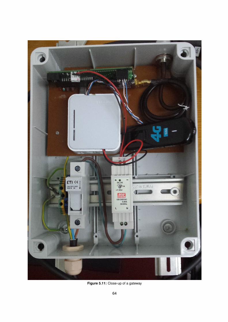
Figure 5.11: Close-up of a gateway
64

Figure 5.12: Deployment of a 3-phase sensor in a pole
Figure 5.13: Close-up of a 3-phase sensor in a pole
65

66

6Conclusion
This report contains the project for the final course work of the author. The author was an active part
of the e-Balance team at INOV and was responsible for the software of the iBee sensors and gateways.
The e-Balance project allowed to validate the sensors in a real deployment.
Managing and maintaining LV grids is becoming increasingly challenging for DSOs due to the complex
layout of the grid and the changing energy demands. With the introduction of Distributed Energy Re-
sources (DER) in the grid, due to low carbon housing regulations, the LV grid has become bidirectional.
The use of voltage and current control in the LV grid has become indispensable to the DSO in order to
manage the grid.
Up to now the DSO has had a passive approach to maintaining the LV grid due to the lack of suitable
equipment to gather the much needed information on the infrastructure’s operational status. Currently
there is a renewed interest and motivation from the DSOs, in the context of Smart Grids, to deploy
network connected sensors along the LV network.
There is no prevalent communication solution is to install a data collector at the secondary substation
and use a polling system to communicate with remote sensors on the grid powered by the substation.
Nowadays, it is not uncommon to find the DSO use PLC to communicate with smart meters located at
67

customers premises, using the feeder cables as the communication medium. However, in the case of
a fault in the feeder, e.g., a short circuit, the communication is lost, while if a wireless communication
solution was used vital information on the fault location and dimension could be obtained.
The sensor and gateway developed in this work are the basis for such a wireless communication system
in the form of a Wireless Mesh Network. The WSN nodes are typically deployed in distribution cabinets
along the streets or in energy poles belonging to the circuits connected to the secondary substations.
The WSN nodes receive query requests and report their data back to a collector via the WSN gateway.
The latter, is placed next to the collector at the secondary substation and here is connected to it through
an Ethernet link.
Communication between the collector and the WSN nodes is based on DLMS, which is the most
common used standard for energy monitoring. In this work a novel implementation of a specification
compliant DLMS/COSEM server is implemented with a focus on low resource usage. The newly de-
veloped DLMS/COSEM server supports 7 different Interface Classes and has 51 OBject Identification
System (OBIS) object implemented. The implementation is easily extended and allows to add new OBIS
to the set, without a large increase in reused resources or efforts.
The communication with the DLMS/COSEM server inside each Wireless Mesh Node is encapsulated in-
side UDP and IPv6 headers. The wireless links of the WMN use 6LoWPAN for IPv6 header compression
and make use of the RPL to support multi hop communication for a robust and self-healing network.
The WSN node is depicted in Figure 6.1 and contains a circuit developed by INOV, which includes
processing and communication modules, voltage/current fault detectors and a temperature sensor. The
author proposed to use the Contiki OS running on a low-cast Atmega MCU with at least 128kB of flash
for the WMN. The WSN nodes developed in e-balance are based on the the XBee Wireless Transceiver
implementing the IEEE 802.15.4 physical layer, operating in the 868 MHz frequency band. The author
also proposed to use a commercially of the shelf OpenWRT capable device for the Wireless Mesh
Gateway, adapted to use with the XBee transceivers. These modules support a raw RF data rate of
24 kbit/s. This results into 2.4 kbit/s of usable data rate due to the mandatory duty cycle of 10%. The
radio range in urban environments can reach a few hundreds of meters, which is easily extended using
multi-hop communications between the WSN gateway and the most distant nodes if needed.
The WSN gateway (see Figure 6.2) connects to the collector through an Ethernet port. Since the collec-
tor does not use IPv6, the gateway also acts as a router between IPv4 and the IPv6 mesh. The gateway
is also equipped with a XBee transceiver and a protocol conversion driver has to be implemented. A
3/4G module is included in the gateway to allow remote access for testing and management purposes,
but is not required to operate the WMN.
The performance of the WSN was considered very good, taking into account the foreseen applications.
A typical RTT of 270.21 ms per hop is obtained, leading to an effective throughput of 2.1 kbit/s. A re-
68

Figure 6.1: Internals of the Wireless Mesh Node
Figure 6.2: Internals of the Wireless Mesh Gateway
69

transmission mechanism implemented at the DLMS level, allowing a maximum of 2 retries per packet,
ensuring a success ratio was higher than 99%.
Three different sensor configurations are supported, which can monitor a single phase, 3 or 4 phases.
All these sensors use the same code-base and the correct selection is based on some configuration
settings, including only the required objects for the configuration. In this work, 51 OBIS objects were
implemented. A proposal was made to extend the COSEM specification with new LV related objects
defined in this work [17].
The developed system was evaluated in a realistic test-bed installed in the Batalha region of Portugal.
Two gateways are installed in two Secondary Substations, see Figure 6.3 and Figure 6.4, monitoring 3
different circuits with a total of 15 Wireless Mesh Nodes.
Figure 6.3: Demonstrator with the secondary substation at Golpilheira
Figure 6.4: Demonstrator with the secondary substation at Jardoeira
During the project, there was an on-site demonstration of the LV Grid monitoring system, where the
project reviewers participated. The wireless monitoring system was extremely well received by the
reviewers, which was confirmed during the final project review.
The author has found working on this solution very rewarding, and has spend copious time debugging
corner cases. This has resulted in a very stable and satisfying solution.
As future work, this type of systems using fixed address schemes for sensors, should allow roaming
schemes of sensors topologies. In this system, if a WMG looses power, all the child nodes are unacces-
sible. It creates a out of reach shadow zone of the grid. It’s a feature of RPL that nodes can join different
70

mesh networks, but these are assigned different IPv6 addresses. In order to nodes keep being identified
as same sensor but with different address, a new registration and joining mechanism should be in place
in Supervisory Control and Data Acquisition (SCADA) application layers. Using power backup systems
in gateways, a DSO would be able to reuse the operational infra-structure on sectional failures of the
grid, and optimize the quality of service.
71

72

Bibliography
[1] eBalance Consortium, “ebalance project website,” 2017, accessed: 2017-11-07. [Online].
Available: http://ebalance-project.eu/
[2] “XBee-PRO 868 - Digi International,” accessed: 2017-11-07. [Online]. Available: http:
//www.digi.com/products/xbee-rf-solutions/modules/xbee-pro-868
[3] “RPL: IPv6 Routing Protocol for Low-Power and Lossy Networks for Linux,” accessed: 2017-11-07.
[Online]. Available: https://github.com/joaopedrotaveira/linux-rpl
[4] A. Dunkels, B. Gronvall, and T. Voigt, “Contiki - A lightweight and flexible operating system for tiny
networked sensors,” Proceedings - Conference on Local Computer Networks, LCN, pp. 455–462,
2004.
[5] A. Dunkels, “Protothreads - Lightweight, Stackless Threads in C. http://dunkels.com/adam/pt/,” no.
March, 2012, accessed: 2017-11-07. [Online]. Available: http://dunkels.com/adam/pt/
[6] “DLMS User Association,” accessed: 2017-11-07. [Online]. Available: http://www.dlms.com
[7] S. Dawans, S. Duquennoy, and O. Bonaventure, “On link estimation in dense RPL deployments,”
Proceedings - Conference on Local Computer Networks, LCN, pp. 952–955, 2012.
[8] J. Lusticky, “Contiki NTP Client,” Ph.D. dissertation, Brno University of Technology, 2012.
[9] D. Mills, J. Martin, J. Burbank, and W. Kasch, “RFC 5905 - Network Time Protocol,”
Internet Engineering Task Force (IETF), pp. 1–111, 2010. [Online]. Available: http:
//www.rfc-editor.org/info/rfc5905
[10] Kalki Communication Technologies Limited, “Implementing DLMS Protocol in Meters,” White Paper.
[11] Electricity metering – Data exchange for meter reading, tariff and load control – Part 6-1: OBIS
Object Identification System, International Electrotechnical Commission (IEC) Std. IEC 62 056-6-1,
2013, originated from DLMS UA - Blue Book.
73

[12] Electricity metering data exchange - The DLMS/COSEM suite - Part 6-2: COSEM interface classes,
International Electrotechnical Commission (IEC) Std. IEC 62 056-6-2, 2013, originated from DLMS
UA - Blue Book.
[13] Electricity metering data exchange – The DLMS/COSEM suite – Part 5-3: DLMS/COSEM applica-
tion layer, International Electrotechnical Commission (IEC) Std. IEC 62 056-5-3, 2013, originated
from DLMS UA - Green Book.
[14] Distribution automation using distribution line carrier systems - Part 6: A-XDR encoding rule, Inter-
national Electrotechnical Commission (IEC) Std. IEC IEC 61 334-6, 2000.
[15] Distribution automation using distribution line carrier systems - Part 4: Data communication pro-
tocols - Section 41: Application protocol - Distribution Line Message Specification, International
Electrotechnical Commission (IEC) Std. IEC 61 334-4-41, 1996.
[16] J. P. Almeida, “D6.3 deployment of demonstrators,” eBalance Consortium, Tech. Rep., 2017.
[17] M. Kuipers, J. P. Taveira, and M. S. Nunes, “ebalance extension to standards,” eBalance Consor-
tium, Tech. Rep., 2016.
[18] Z. Fan, P. Kulkarni, S. Gormus, C. Efthymiou, G. Kalogridis, M. Sooriyabandara, Z. Zhu,
S. Lambotharan, and W. H. Chin, “Smart Grid Communications: Overview of Research
Challenges, Solutions, and Standardization Activities,” pp. 1–19, 2011. [Online]. Available:
http://arxiv.org/abs/1112.3516
[19] X. Fang, S. Misra, G. Xue, and D. Yang, “Smart Grid – The New and Improved Power Grid:
A Survey,” IEEE Communications Surveys & Tutorials, vol. Preprint, pp. 1–37, 2011. [Online].
Available: http://ieeexplore.ieee.org/xpls/abs all.jsp?arnumber=6099519
[20] I. H. Cavdar, “A solution to remote detection of illegal electricity usage via power line communica-
tions,” IEEE Transactions on Power Delivery, vol. 19, pp. 1663–1667, 2004.
[21] M. Nassar, J. Lin, Y. Mortazavi, A. Dabak, I. H. Kim, and B. L. Evans, “Local utility power line
communications in the 3-500 kHz band: Channel impairments, noise, and standards,” IEEE Signal
Processing Magazine, vol. 29, no. 5, pp. 116–127, 2012.
[22] H. C. Ferreira, L. Lampe, J. Newbury, and T. G. Swart, Power Line Communications: Theory and
Applications for Narrowband and Broadband Communications over Power Lines, 2010.
[23] ITU-T, “G.9955 Narrowband orthogonal frequency division multiplexing power line communication
transceivers - Physical layer specification,” 2011.
74

[24] ——, “G.9956 - Narrowband orthogonal frequency division multiplexing power line communication
transceivers - Data link layer specification,” 0.
[25] IEEE, “1901.2-2013 - IEEE Standard for Low-Frequency (less than 500 kHz) Narrowband
Power Line Communications for Smart Grid Applications,” 2013. [Online]. Available: http:
//ieeexplore.ieee.org/servlet/opac?punumber=6679208
[26] ITU-T, “G.9963 Unified high-speed wireline-based home networking transceivers - Multiple input/-
multiple output specification.”
[27] IEEE, IEEE Std 802.16j-2009: IEEE Standard for Local and metropolitan area networks Part 16:
Air Interface for Broadband Wireless Access Systems, 2009.
[28] B. Lichtensteiger, B. Bjelajac, C. Muller, and C. Wietfeld, “RF Mesh Systems for Smart Metering:
System Architecture and Performance,” Smart Grid Communications (SmartGridComm), 2010 First
IEEE International Conference on, pp. 379–384, 2010.
[29] V. Gungor, B. Lu, and G. Hancke, “Opportunities and Challenges of Wireless Sensor Networks in
Smart Grid,” IEEE Transactions on Industrial Electronics, vol. 57, no. 10, pp. 3557–3564, 2010.
[Online]. Available: http://ieeexplore.ieee.org/ielx5/41/5567234/05406152.pdf?tp=&arnumber=
5406152&isnumber=5567234
[30] B. Akyol, H. Kirkham, S. Clements, and M. Hadley, “A survey of wireless communications for the
electric power system,” Prepared for the US Department of Energy, no. January, pp. 1–33, 2010.
[Online]. Available: https://www.pnnl.gov/nationalsecurity/technical/secure cyber systems/pdf/
power grid wireless.pdf
[31] N. Saputro, K. Akkaya, and S. Uludag, “A survey of routing protocols for smart grid
communications,” Computer Networks, vol. 56, no. 11, pp. 2742–2771, 2012. [Online]. Available:
http://www.sciencedirect.com/science/article/pii/S1389128612001429
[32] IEEE, IEEE Standard for Information technology–Telecommunications and information exchange
between systems Local and metropolitan area networks–Specific requirements Part 11: Wireless
LAN Medium Access Control (MAC) and Physical Layer (PHY) Specifications, 2012, vol. 2012, no.
March. [Online]. Available: http://ieeexplore.ieee.org/servlet/opac?punumber=6178209
[33] C. Perkings, E. Belding-Royer, and S. Das, “Ad hoc On-Demand Distance Vector (AODV) Routing,”
IETF RFC 3561, pp. 1–37, 2003. [Online]. Available: http://tools.ietf.org/pdf/rfc3561.pdf
[34] T. Clausen and P. Jacquet, “RFC 3626 - Optimized Link State Routing Protocol (OLSR),” p. 75,
2003.
75

[35] T. Winter, P. Thubert, A. Brandt, T. H. Clausen, J. W. Hui, R. Kelsey, P. Levis,
K. Pister, R. Struik, and J. Vasseur, “Rpl: Ipv6 routing protocol for low power and lossy
networks,” Work In Progress), http://tools. ietf. org/html/draft-ietf-roll-rpl-19, no. July, pp. 1–164,
2011. [Online]. Available: http://scholar.google.com/scholar?hl=en&btnG=Search&q=intitle:
RPL:+IPv6+Routing+Protocol+for+Low+power+and+Lossy+Networks#0
[36] Nist, N. S. Publication, and National Institute of Standards and Technology, “NIST
Special Publication 1108 NIST Framework and Roadmap for Smart Grid Interoperability
Standards,” Nist Special Publication, vol. 0, no. October, pp. 1–90, 2010. [Online]. Available:
http://www.nist.gov/public affairs/releases/upload/smartgrid interoperability final.pdf
[37] H. Farhangi, “The path of the smart grid,” IEEE Power and Energy Magazine, vol. 8, no. 1, pp.
18–28, 2010.
[38] P. Yi, A. Iwayemi, and C. Zhou, “Developing ZigBee deployment guideline under WiFi interference
for smart grid applications,” IEEE Transactions on Smart Grid, vol. 2, no. 1, pp. 98–108, 2011.
[39] IEC, “IEC 61970: Energy management system application program interface (EMS-API): Part 301:
Common information model (CIM) base,” 2009.
[40] P. Kulkarni, S. Gormus, Z. Fan, and B. Motz, “A mesh-radio-based solution for smart
metering networks,” IEEE Communications Magazine, vol. 50, no. 7, pp. 86–95, 2012.
[Online]. Available: http://ieeexplore.ieee.org/ielx5/35/6231266/06231284.pdf?tp=&arnumber=
6231284&isnumber=6231266
[41] “Smart Grid Standards,” Silver Spring Networks, no. whitepaper, 2012.
[42] EUTC, “Spectrum needs for Utilities EUTC position paper,” no. 1.0. [Online]. Available:
http://eutc.org/system/files/UTC private file/EUTCSpectrumPositionPaper-9April2013.pdf,
76
AMonitorBT: Survey on
communications technologies
In the recent past, the concept of Smart Grid has gained relevance as a paradigm for the future energy
grids. In Portugal, in the year of 2008, EDP Distribuicao launched the InovGrid project with the support
of Portuguese industrial and scientific partners, focused on the development of a fully active distribution
network based on a smart grid infrastructure, following the need to introduce more intelligence to man-
age and control distribution networks with large-scale integration of micro-generation and responsive
loads. The InovGrid project encompasses the deployment of a test site in Evora, Portugal (Inovcity),
where a smart grid infrastructure exploiting different ICT solutions was implemented with more than
30’000 smart meters. A reference architecture for smart grids, shown in Figure A.1, has been devel-
oped within the framework of InovGrid, encompassing all the chain elements of the distribution system.
This architecture is based on a hierarchical control approach in which each control layer is able to collect
and process data related to the operation of the network downstream. This is supported by the commu-
nication infrastructure that enables refreshing and/or updating the status of the network since all layers
77

have pre-processing capabilities. This structure follows closely the organization of the physical distribu-
tion grid. At the top level, central systems such as the SCADA / Distribution Management System (DMS)
manage the whole distribution network through two intermediate control layers:
• One control layer at the HV/ MV substation level, where a Smart Substation Controller (SSC)
manages the MV network through a set of control functionalities, including several DER that are
directly connected at the MV level;
• One control layer at the MV/ LV substation level with a DTC that is in charge of the LV network,
managing a set of LV prosumers (clients that not only consume energy but also produce energy
through µG) via the corresponding smart meter, which, within InovGrid, is known as energy box
Energy Box (EB).
Figure A.1: InovGrid System Architecture.
The EB and the DTC are the main components of the InovGrid infrastructure. The EB is a device
installed at the consumer / producer premises that includes a measurement module, control module and
communications module. The DTC is a local control device installed in MV/ LV secondary substations
comprising a measurement module, control module and communications module. It collects data from
EBs and MV/ LV substation and performs data analysis functions, monitors the grid and provides an
interface with commercial and technical central systems.
78

Several communication technologies have been presented in the literature as candidates to provide
the underlying support for the Smart Grid functionalities. However, given the dimension, complexity
and scenario diversity of the Smart Grid, it is doubtful that the market will converge to a single winner,
since all technologies have advantages and disadvantages with respect to this or that evaluation metric
or scenario peculiarity. In fact, some published papers consider the possibility of integrating several
technologies, from low-rate short-range wireless communications to fiber optic segments capable of
aggregating data rates in the order of Mbit/s or Gbit/s spanning distances in the order of many kilometres
[18,19].
Monitor BT final solution aims to sensorize and monitor utility’s field devices, as well as to control µG
equipment at the customer premises, with both of them being located in the LV section of the electricity
distribution grid. In terms of the InovGrid architecture, this corresponds mainly to the Local Area Network
(LAN) section of the communications infrastructure.
Although some of the sensor data is to be monitored by remote central systems - which also involves
the Wide Area Network (WAN) - the project shall here rely on existing communications infrastructure.
This state-of-the-art will thus restrict its scope to the technologies that are considered suitable for LAN
deployment:
• PLC
• Infrastructure-based Wireless Networks
• RF-Mesh
The reasons why these technology groups are here more relevant have mainly to do with the following
factors:
• Since the LAN is already located at the edge of the Smart Grid, the amount of traffic is much lower
in comparison with the WAN, since the latter must aggregate traffic from several LAN islands.
• For cost-effectiveness reasons, the footprint of the communications network in terms of additional
equipment and/or requirement for changes in existing grid equipment must be minimized. Wireless
technologies avoid the deployment of cabled infrastructure RF-Mesh or employ existing infrastruc-
ture from a telecom operator (Public Land Mobile Network (PLMN)). On the other hand, PLC also
avoids the deployment of cabled infrastructure, since the latter already exists in the electricity grid.
This document shall analyse these three groups of candidate technologies, presenting their advantages,
disadvantages and constraints.
79

A.1 Power Line Communications (PLC)
This technology is used since the 1950s by the electricity distribution companies in order to remotely
perform some control functions on electric network equipment [20]. Recently, this technology has earned
more relevance because the technology evolution has led to an increase of the achieved data rates,
both in medium and low voltage. The advantage of PLC comes from the fact that it uses the same
infrastructure for both energy distribution and communications, which greatly reduces the deployment
costs.
The PLC systems are usually classified according to three different bandwidth classes: Ultra Narrow-
band (UNB), Narrowband (NB) and Broadband (BB) [21, 22]. Although the attained data rates and
ranges are highly dependent on the specific characteristics and transient conditions of the network (e.g.,
the impedance is highly dependent on the number and characteristics of attached electrical devices),
some approximate figures shall be provided as a reference to allow a better comparison between the
different classes.
The UNB-PLC systems operate in the Very Low Frequency (VLF) band, which corresponds to 0.3-3.0
kHz. The attained bit rates are usually in the order of 100 bit/s, with ranges of up to 150 km. The relevant
UNB-PLC applications comprise Automatic Meter Reading (AMR), fault detection in the distribution grid,
as well as voltage monitoring.
The NB systems operate in the Low Frequency (LF) band, which corresponds to 3-500 kHz. In Europe,
the European Committee for Electrotechnical Standardization (CENELEC) has defined four frequency
bands for PLC use: CENELEC-A (3-95 kHz), CENELEC-B (95-125 kHz), CENELEC-C (125-140 kHz)
and CENELEC-D (140-148.5 kHz). CENELEC-A is reserved for exclusive use by energy providers,
while CENELEC-B, CENELEC-C and CENELEC-D are open for end user applications. In the USA, the
Federal Communications Commission (FCC) has specified operation in the 10-490 kHz frequency band.
In Japan, the Association of Radio Industries and Businesses (ARIB) band was defined in the range 10-
450 kHz, while in China an unregulated single band in the range 3-500 kHz was defined, with a sub-band
in the range 3-90 kHz being preferred by China’s Electric Power Research Institute (CEPRI). In NB-PLC,
the attained data rates span from a few kbit/s to around 800 kbit/s - depending on the technology, band-
width and channel conditions - while the range is in the order of some kilometres. Some standards for
Building Automation Applications (BAA), such as BacNet (ISO 16484-5) and LonTalk (ISO/IEC 14908-3),
employ NB-PLC with a single carrier. The IEC 61334 standard for low-speed reliable power line com-
munications by electricity meters, water meters and SCADA, uses the 60-76 kHz frequency band, being
able to achieve 1.2-2.4 kbit/s with Spread Frequency Shift Keying (S-FSK) modulation. Yitran Communi-
cations Ltd. and Renesas Technology provide solutions based on Differential Chaos Shift Keying (DCSK)
- a form of Direct-Sequence Spread Spectrum (DSSS) -, which are able to achieve bitrates as high as 60
80

kbit/s in the CENELEC-A band. On the other hand, PoweRline Intelligent Metering Evolution (PRIME)1
and G32 are multi-carrier systems based on Orthogonal Frequency Division Multiplexing (OFDM), which
allows them to support higher data rates. PRIME operates within the CENELEC-A frequency band,
more specifically in the 42-89 kHz range, and is able to achieve 21-128 kbit/s. G3 may operate in the
CENELEC-A, CENELEC-B, ARIB and FCC bands, being able to achieve 2.4-46 kbit/s. The G3-PLC
Media Access Control (MAC) layer is based on the IEEE 802.15.4 MAC. In order to unify the OFDM-
based NB-PLC systems, International Telecommunication Union (ITU) has approved recommendations
G.9955 (G.hnem physical layer) [23] and G.9956 (G.hnem data link layer) [24], while IEEE has approved
standard P1901.2 [25].
BB-PLC systems operate in the High Frequency (HF) and Very High Frequency (VHF) bands, which
corresponds to 1.8-250 MHz. The achievable data rates may be as high as 500 Mbit/s, but the range
is significantly (about ten times) shorter than for NB-PLC. Consequently, BB-PLC is usually used for
local connectivity in the Home Area Network (HAN) or as a broadband access technology. The most
recent BB-PLC standards are IEEE P1901 also designated Broadband Over Power Line (BPL)3 and ITU
G.996x (G.hn), which are based on OFDM. The ITU G.9963 recommendation [26] also incorporates
some multiple-input and multiple-output (MIMO) concepts through the use of multiple cables.
Despite the advantages of PLC for Smart Grid applications, namely the reduced costs and easier man-
agement of a single infrastructure (i.e. energy distribution plus communications in a single network),
PLC faces many obstacles and challenges, which are often similar to the ones faced by RF-Mesh (see
below):
• The shared medium is subject to significant attenuation and noise, which limit the data rates and
ranges that can be effectively achieved. The shared medium is also the cause of security issues,
since it is very easy to plug a device to the LV section of the grid.
• A failure in the energy distribution infrastructure usually means that the communications cannot
take place while the malfunction rests unresolved, which may negatively affect some applications.
Another consequence of the latter is that a communications failure may be wrongly interpreted as
a malfunction in the energy distribution infrastructure.
A.2 Infrastructure-based Wireless Networks
The technologies that fall on this category rely on a fixed infrastructure of base stations, together with
switching equipment and management systems in order to provide wide coverage communications ser-
vice to the end user. Fixed wireless access and mobile cellular networks, both fit into this category.1PoweRline Intelligent Metering Evolution: http://www.prime-alliance.org2http://www.maxim-ic.com/products/powerline/g3-plc3IEEE P1901 is based on the HomePlug AV system developed by the HomePlug Powerline Alliance
81

The WiMAX technology is defined in the IEEE 802.16 standard for fixed and mobile broadband wireless
access [27], being able to achieve a coverage range in the order of 50 km and data rates in the order
of tens or even hundreds of Mbit/s. Despite its advantages, the widespread adoption of Long-Term
Evolution (LTE) by mobile operators has brought down the initial popularity that WiMax was for some
time able to enjoy. Moreover, the lack of WiMax networks and operators in Portugal constitutes significant
obstacles to the adoption of this technology to support Smart Grid functionalities in this country, since
the energy provider would have to deploy its own WiMax infrastructure. WiMAX shall be addressed
again in this document, but in the context of RF-Mesh technologies.
The mobile cellular communications technologies divide the covered territory into smaller areas desig-
nated cells, each served by a base station. If the base station is equipped with directional antennas,
the cell may be further sectorized, which increases the frequency reuse and hence its capacity to sup-
port more users. Before a call is established, the mobile user terminal is tracked as it moves between
different sectors or cells, allowing the mobile terminal to be paged at any time. Moreover, handover sig-
nalling procedures allow the user to move even while a call is taking place. Mobile cellular technologies
have already spanned three digital generations starting on the 2nd Generation (2G) and are already in
their fourth generation. Examples of 2G technologies available in Europe (and Portugal in particular) are
Global System for Mobile Communications (GSM)/General Packet Radio Service (GPRS) and Terrestrial
Trunked Radio (TETRA). GPRS is the packet switched complement of GSM and supports effective data
rates up to 177.6 kbit/s in the downlink and 118.4 kbit/s in the uplink. The effective data rate depends on
the required error protection, class of terminal and sharing with other users using the same frequency
channel. The TETRA technology is primarily used by security and civilian protection entities, as well
as transportation services, due to the support of specific functionalities like direct mode operation and
group calls. The supported data rates span from 2.4 kbit/s to 28 kbit/s, depending on the required error
protection and channel allocation.
The 3G arrived in the beginning of this century with the Universal Mobile Telecommunication Sys-
tem (UMTS), which offered 2 Mbit/s (shared) in urban areas. UMTS suffered a number of upgrades
to increase the supported data rates, namely the High-Speed Downlink Packet Access (HSDPA) and
HSDPA+ for the downlink, and High-Speed Uplink Packet Access (HSUPA) for the uplink. HSDPA is
offered with data rates up to 42 Mbit/s, though later releases specify higher data rates up to 337 Mbit/s
with HSDPA+. In the opposite direction, HSUPA supports data rates up to 23 Mbit/s, though existing
mobile operators have not offered more than 5.76 Mbit/s.
CDMA450 is also a 3G technology, based on the adaptation of the American standard CDMA2000 to
operate in the 450-470 MHz frequency band. The supported total bitrates depend on the specific mode
of operation. For Multicarrier EV-DO, overall bitrates may be as high as 9.3 Mbps for downlink and 5.4
Mbps for uplink, with average rates per user in the order of 1.8-4.2 Mbps for downlink and 1.5-2.4 Mbps
82

for uplink. This technology was offered in Portugal by the Zapp operator until 2011, being abandoned
afterwards. This means that in order to use CDMA450 as a Smart Grid infrastructure, the utility will have
to deploy its own network infrastructure, like for WiMax. Currently, most European mobile operators
already offer LTE, including the Portuguese mobile operators. Although marketed as 4G, LTE does not
satisfy all the 4G requirements defined by 3GPP, being instead classified as a 3.9G technology. LTE
employs Orthogonal Frequency Division Multiple Access (OFDMA) in the downlink and Single-Carrier
Frequency Division Multiple Access (SC-FDMA). Supported peak data rates are 299.6 Mbit/s for the
downlink and 75.4 Mbit/s for the uplink.
Given their proven reliability, technology maturity and extensive coverage, mobile cellular networks con-
stitute important candidates to support the Smart Grid communications infrastructure, being used al-
ready in applications such as AMR. However, these technologies face the following challenges:
• The difficulties related with RF penetration inside buildings constitute sometimes an obstacle for
its use for some Smart Grid applications, namely AMR.
• The fact that the mobile cellular network is most of the time managed by an external opera-
tor, means that the utility will have to pay the latter for the provisioning of communications ser-
vices. Alternatively, the utility might deploy its own communications infrastructure (e.g., WiMax
or CDMA450), though that would certainly constitute a substantial investment on communication
systems.
A.3 Radio-frequency Mesh (RF-Mesh)
An RF-Mesh is a network formed by RF capable nodes, which are self-organized in a mesh topol-
ogy [28–31]. This self-organization capability brings several advantages in the context of Smart Grid
communications, namely deployment flexibility and automatic connection re-establishment and topology
reconfiguration in the presence of link or node failure. This explains why this family of technologies is so
popular in the USA, where it is used to support Smart Metering applications. Within the RF-Mesh family,
we can distinguish between broadband and narrowband technologies.
The most representative broadband technologies are currently WiFi [32] and IEEE 802.16j [27]. Even
if the IEEE 802.11s mesh extension is not used, IEEE 802.11 can be configured to operate as a mesh
by performing ad-hoc routing at the network layer (e.g., IP layer). These technologies support com-
munication ranges in the order of hundreds (IEEE 802.11) or thousands (IEEE 802.16) of meters, as
well as high data rates in the order of Mbit/s, which makes them multimedia capable. Besides physi-
cal and MAC aspects, IEEE 802.11s specifies the routing protocol, which is the Hybrid Wireless Mesh
Protocol (HWMP). The latter is a hybrid between a tree routing protocol and the Ad-hoc On-Demand
Distance Vector (AODV) protocol [33]. In case IEEE 802.11 is used without the mesh extension, a myr-
83

iad of routing protocols such as AODV, OLSR [34], or RPL [35] can be used at the network layer. As to
IEEE 802.16j, it does not specify how the path evaluation and selection is done, there being freedom for
manufacturer specific implementations. However, it constrains the topology to be tree based. Although
the high bitrates supported by broadband RF-Mesh allow the support of virtually any Smart Grid appli-
cations, both real-time and non-real-time, these technologies also have some disadvantages that can
hinder their global applicability:
• Broadband communications means operating at higher frequencies, which are more vulnerable to
path loss and other causes of signal attenuation.
• Broadband RF-Mesh transceivers often present higher energy consumption in comparison with
narrowband RF-Mesh. This is made even worse by the need to increase the transmit power in
order to compensate for path loss and attenuation. The deployment of a huge number of nodes
means that the energy overhead introduced by the Smart Grid communications may start to be
non-negligible.
• High bitrates demand a corresponding processing and storage capacity to be available on the
network nodes, which will likely be translated into an increase of the unit cost.
• The deployment of these technologies by the utility requires the choice of the operating frequency.
IEEE 802.11 operates mainly on the unlicensed bands of 2.4 GHz or 5 GHz. The 2.4 GHz band
is cluttered, since it is subject to the interference of both private and public Wireless Local Area
Network (WLAN)s. On the other hand, the 5 GHz band has a reduced range for the same transmit
power. IEEE 802.16 supports frequency bands between 2 GHz and 66 GHz, both licensed and
unlicensed. Besides the problems related with spectrum occupancy, the use of unlicensed bands
also raises the problem of communications security. On the other hand, the use of licensed bands
usually represents additional costs for the utility.
The narrowband RF-Mesh technologies correspond to those that belong to the WSN and IoT domains.
These are usually characterized by simpler hardware and operating systems, leading to a lower unit
cost [29]. The lower power consumption that characterizes these technologies allows greater autonomy
and effectiveness of energy harvesting techniques, which can feed the network nodes in case they
cannot be directly fed by the LV network (e.g., MV power line sensors).
In the context of WSNs, the IEEE 802.15.4 standard is nowadays prominent, constituting the base
(Physical Layer Protocol (PHY) and MAC layers) of several protocol stacks such as ZigBee, Wire-
lessHART, ISA100.11a and IoT, which are recommended for industrial and Smart Utility Networks (SUN)
applications [30]. The IEEE 802.15.4 MAC protocol is based on Carrier Sense Multiple Access with Col-
lision Avoidance (CSMA/CA), but also includes an optional Time Division Multiple Access (TDMA) op-
erational mode. The latter is reserved for traffic that requires stringent access delay guarantees. While
84

the original IEEE 802.15.4 standard restricted operation to the unlicensed frequency bands of 868-870
MHz (Europe), 902-928 MHz (USA) and 2.4 GHz, the IEEE 802.15.4g standard for SUN extends the set
of supported Ultra-High Frequency (UHF) bands, adds new transmission modes (e.g., OFDM) and ex-
tends the MAC layer functionalities to allow the efficient and fair coexistence of networks using different
transmission modes within the same frequency range. IEEE 802.15.14g can achieve a maximum bitrate
of 1094 kbit/s and maximum ranges in the order of tens of kilometres.
ZigBee is a standard protocol stack brought forth by the ZigBee Alliance consortium, which includes
IEEE 802.15.4 at the lower layers, but defining its own network and application support layers. ZigBee,
together with its ZigBee Smart Energy application profile, were defined by the National Institute of Stan-
dards and Technology (NIST) in USA as standards for communications within the HAN domain of the
Smart Grid [36]. ZigBee was also selected by many energy companies as the communication technol-
ogy for smart meters, since it provides a standard platform for data exchange between the latter and
HAN devices [37]. The functionalities supported by the Smart Energy profile include load management,
AMR, real-time billing and text messaging [38]. The ZigBee Alliance also developed an IP networking
specification called ZigBee IP which is based on existing Internet Engineering Task Force (IETF) proto-
cols defined for IoT (see below). The ZigBee Smart Energy version 2.0 specifications already make use
of ZigBee IP. It is an enhancement of the ZigBee Smart Energy version 1 specifications, adding services
for Plug-in Electric Vehicle (PEV) charging, installation, configuration and firmware download, prepaid
services, user information and messaging, load control, demand response and common information
and application profile interfaces for wired and wireless networks. The application function sets imple-
mented in this release were mapped to the International Electrotechnical Commission (IEC) Common
Information Model (CIM) [39].
WirelessHART is another protocol stack, based on a TDMA MAC protocol, being IEEE STD 802.15.4-
2006 compatible at Physical Layer and MAC Protocol Data Unit (PDU). It was developed as an adap-
tation of the HART protocol defined for wired industrial networks. While it was initially developed by a
private consortium, the stack was standardized by the IEC as IEC 62591. ISA100.11a is a standard
protocol stack developed by the International Society for Automation (ISA), which is functionally very
similar to WirelessHART [30].
In the meantime, IETF has defined a protocol stack adapted to the characteristics of the IoT, which is
suitable to support Smart Grid applications in a way that is more compatible with the standard Internet
Protocol stack [40]. The core of the IoT protocol stack is 6LoWPAN, which specifies how to support
the IPv6 protocol over low bitrate wireless technologies, such as IEEE 802.15.4. 6LoWPAN specifies
the protocols and procedures needed for address assignment and deconfliction, IPv6 and higher layer
header compression and fragmentation. Energy efficiency lies at the core of 6LoWPAN. Header com-
pression exploits the redundancy between the MAC and IPv6 header fields - namely the addresses -,
85

and/or simplifies the range of IPv6 header field value options in order to achieve higher compression
rates. Regarding the routing function, the ROLL group in IETF has specified the already mentioned RPL
protocol [35]. RPL is based on the formation of routing trees designated Destination Oriented Directed
Acyclic Graphs (DODAGs), supporting the overlapping between two or more of these, possibly with dif-
ferent root nodes. RPL is designed to minimize the routing overhead in stable networks, which is done
by increasing the routing message period exponentially when there are no topology changes. On the
other hand, the protocol keeps its responsiveness to topology changes by restoring the initial routing
update period once a topology change is detected. As already seen, ZigBee Smart Energy version 2.0
already takes advantage of these IP-oriented functionalities.
Besides the standard RF-Mesh solutions described above, there are a number of proprietary RF-Mesh
solutions that were developed in the USA and have been enjoying significant popularity among energy
operators. These products usually operate within the Industrial, Scientific and Medical (ISM) frequency
band of 902-928 MHz and employ Frequency Hop Spread Spectrum (FHSS) to increase the robustness
and security of the links, namely to prevent jamming attacks and interference from other equipment
operating in the same ISM band. Offered bitrates range between 9.6 kbps and 300 kbps, with ranges in
the order of 2 km with 1 W of transmit power. An example is the Landis+Gyr’s Gridstream, which employs
a proprietary geographical based routing protocol in order to minimize the routing overhead [28]. Another
example is the Silver Spring Networks solution [41], which is used in the InovGrid project (see below).
The advantages of narrowband RF-Mesh solutions are mostly related with deployment flexibility, in-
creased range and use of less cluttered ISM frequency bands such as the 900 MHz in the USA and 868
MHz in Europe. The main disadvantage is, of course, the reduced bitrates as compared with broadband
RF-Mesh solutions.
Some additional disadvantages can be identified for RF-Mesh solutions in general, which are the follow-
ing:
• Performance is highly dependent on the propagation and interference environment.
• Depending on the scenario and inter-node distances, the deployment of additional relay nodes
may be needed, which adds to the deployment costs.
• Wireless communications propagate through a shared medium, which poses significant threats
in terms of security. The protocol stack must implement security mechanisms that are able to
meet the requirements of the Smart Grid applications. These requirements are often different from
application to application.
It should be noted that the European Utilities Telecom Council (EUTC) is seeking to reserve 6 MHz in
the 450-470 MHz frequency band for use by grid utility operators, together with a frequency band above
1 GHz (e.g., 1.5 GHz band spanning 10 MHz) [42]. In this way, both low rate and high rate applications
86

would be supported.
A.4 Summary
This chapter has presented the state-of-the-art of communication technologies for the Smart Grid, fo-
cusing on the LAN section of the InovGrid architecture reference model. Three types of communication
technologies were analysed: PLC, Infrastructure-based Wireless Networks and RF-Mesh. The main
characteristics of these technologies are listed in Table A.1, as well as the results of InovGrid perfor-
mance tests for the tested technologies, in order to facilitate the comparison.
Table A.1: Comparison between Smart Grid LAN communication Technologies
Type Subtype CAPEX OPEX MaximumBitrate
Rangea
InovGridPerfor-mance
test(Serv. Load
Diagram)
InovGridPerfor-mance
test(Serv. DailyTotalizers)
PLC UNB Low Negligible 100 bit/s 150 km
NB Low Negligible 128 kbit/s(CENELEC-A) Several km
1m26sec(PRIME)3m12sec(DCSK)
17sec(PRIME)
45sec(DCSK)
Infrastructure-based
WirelessNetworksb
2.5G(GPRS) Low High
177.6 kbit/sdownlink
118.4 kbit/suplink
Coveragedepen-
dent1m10sec 31sec
3G(HSDPA,HSUPA)
Low High
42 Mbit/sdownlink
5.76 Mbit/suplink
Coveragedepen-
dent
4G(WiMAX,
LTE)Low High
299.6 Mbit/sdownlink
75.4 Mbit/suplink
Coveragedepen-
dent
RF-Mesh
Broadband(IEEE
802.11n/s)High Negligible 600 Mbit/s Hundreds
of meters
Narrowband(SilverSpring
Networks)
High
High (iflicense isrequired
fromANA-
COM4)
100 kbit/s Several km 1m02sec 17s
Narrowband(IEEE
802.15.4g)Medium Negligible 1094 bit/s
Severalkm
(e.g.XbeePro868 @
24kbit/s [2])
a Maximum ranges usually achieved with the lowest bitrates only.b Assumed hired from a Service Provider.
From the Table A.1, it can be concluded that NB RF-Mesh and NB PLC offer the best compromise
87

between bitrate, range and cost, especially if the supported Smart Grid services require a low bitrate.
Mobile cellular solutions are easy to deploy, since mobile cellular coverage is very extensive. However
this communications service must be paid to the operator, which may result into significant operational
costs.
88

BBandwidth Estimation Tests
The Sensor nodes are low-power nodes, with limited processing capacity and memory as compared to
the average desktop computer. The sensor nodes do not have any special bandwidth measurements
software, limiting the options to obtain bandwidth estimates to passive procedures, such as the ones
here using ping-commands. Two different, but related, procedures have been used to estimate the
bandwidth of the link.
B.1 Procedure 1: Ping-test
In this test, a fixed size ping packet is sent and the round-trip times are used to calculate the throughput.
The formula used to estimate the bandwidth, Cp1, is:
Cp1 =8L
1000Trtt[kb/s] (B.1)
where L is the packet-size in bytes (including headers) and Trtt is the measured round-trip time. The
packet-size is multiplied by 8 to obtain the packet size in bits. The result divided by 1000 in order to
89

show the results in the more common unit of kb/s.
In order to prevent fragmentation, the fixed packet size (including headers) needs to be less than the
frame-size of the MAC layer. The packet-size is set to 60 bytes. The disadvantage of this test is that the
round-trip time includes the processing time of the ICMP Echo Request in the sensor-node, however, it
is very easy and fast to perform.
B.2 Procedure 2: Differential Ping-test
This test aims to eliminate the processing overhead of the ICMP Echo Request in the sensor-node by
transmitting a small and a large-size ping packet and using the differences. The formula to estimate the
bandwidth, Cp2, is given by
Cp2 =8(Lb − Ls)
1000(Trtt,b − Trtt,s)[kb/s] (B.2)
Where Ls and Lb are the packet-sizes for the small and big packet, respectively. The round-trip time
for the small packet-size is given by Trtt,b and by Trtt,s for the large packet-size. The small-size ping
packet, Ls, is set to 20 bytes, whereas the large-size ping packet, Lb, is set to 60 bytes (same as in
Procedure 1).
90

CCode
C.1 Non-graceful Reboot Test Script
1 #!/usr/bin/python23 import sys4 import getopt5 import time6 import serial7 import os8 import ping69 import subprocess
1011 usage_string = 'usage: boot.py -s <serialport> -l <localipv6>'1213 node_array = []14 node_array.append([])15 node_array[0].append('aaaa::213:a200:4094:5c60')16 node_array[0].append('aaaa::213:a200:408b:c99d')17 node_array[0].append('aaaa::213:a200:408b:c95a')18 node_array[0].append('aaaa::213:a200:408b:c999')1920 def main(argv):21 serialport = ''22 remoteip = ''23 localip = ''24 logfile = 'boot_gw_mult_multihop.log'25 try:26 opts, args = getopt.getopt(argv,"hs:l:",["port=", "localip="])27 except getopt.GetoptError:28 print usage_string29 sys.exit(2)30 if len(sys.argv) < 5:31 print usage_string32 sys.exit(2)33
91

34 for opt, arg in opts:35 if opt == '-h':36 print usage_string37 sys.exit()38 elif opt in ("-s", "--port"):39 serialport = arg40 elif opt in ("-l", "--localip"):41 localip = arg4243 print 'Serial Port is ', serialport44 print 'Local IPV6 is ', localip4546 # configure the serial connections (the parameters differs on the device you are connecting to)47 ser = serial.Serial(48 port=serialport,49 baudrate=9600,50 parity=serial.PARITY_NONE,51 stopbits=serial.STOPBITS_ONE,52 bytesize=serial.EIGHTBITS53 )5455 if ser.isOpen() == True:56 ser.close();57 try:58 ser.open()59 except Exception, e:60 print "error opening serial port: " + str(e)61 sys.exit(2)6263 # open log file64 if os.path.isfile(logfile):65 os.remove(logfile)6667 file = open(logfile, "w")68 logstring = "#start: " + time.strftime("%Y-%m-%d %H:%M:%S", time.localtime()) + '\n'69 file.write(logstring)70 print logstring7172 retries = 173 timeout = 074 control = 17576 # turn power on77 ser.write('l')78 #time.sleep(15) # 15 seconds wait79 starttime = time.time();8081 try:82 while retries < 1001:83 for i in range(len(node_array[0])):84 print node_array[0][i]85 resulttime = time.time();8687 while 1:88 file.flush()89 # ping for each PING_PERIOD seconds untill an answer or timeout90 result = 091 pingtime = time.time();92 result = ping6.ping(localip, node_array[0][i])9394 # got answer95 if result:96 timeout = 097 endtime = time.time();98 totaltime = int(endtime - starttime)99 epoch = int(time.time() - 946684800)
100 logstring = str(epoch) + ',' + node_array[0][i] + ',' + str(retries) + ','+ str(totaltime) + ',' + str(int(endtime - resulttime)) + ',' + 'OK' +'\n'
→→
101 file.write(logstring)102 print logstring103 break;104 # no answer105 else:106 while (time.time() - pingtime) < 10:107 time.sleep(1) # N seconds wait108 timeout = int(time.time() - resulttime)109 if timeout > 180:110 endtime = time.time();111 totaltime = int(endtime - starttime)112 epoch = int(time.time() - 946684800)113 logstring = str(epoch) + ',' + node_array[0][i] + ',' + str(retries) +
',' + str(totaltime) + ',' + str(timeout) + ',' + 'ERROR' + '\n'→114 file.write(logstring)115 print logstring116 break117118 if control == 0:119 break120 if control == 0:
92

121 break122 if control == 0:123 break124 file.flush()125 ser.write('d')126 time.sleep(30)127 retries = retries + 1;128 # turn power on again129 ser.write('l')130 starttime = time.time();131132 except KeyboardInterrupt:133 # abort134 logstring = "#aborted: " + time.strftime("%Y-%m-%d %H:%M:%S", time.localtime()) + '\n'135 file.write(logstring)136 print logstring137 control = 0138139 logstring = "#end: " + time.strftime("%Y-%m-%d %H:%M:%S", time.localtime()) + '\n'140 file.write(logstring)141 print logstring142143 ser.write('d')144145 file.close()146147 if __name__ == "__main__":148 main(sys.argv[1:])
Listing C.1: Non-graceful Reboot test script
93

C.2 Complete List of COSEM objects
1 #ifndef DLMS_OBJECTS_H_2 #define DLMS_OBJECTS_H_34 #include <dlms-types.h>56 /* Objects List for DEBUG purposes */7 #if 0 && defined MBTSENSOR8 #define OBIS_OBJECTS \9 /* Sensor Transmission Power */ \
10 OBIS(3,0,0,67,128,9,255,AT_DOUBLE_LONG) \11 /* Current Alarm Phase 1 */ \12 OBIS(67,0,0,67,128,0,255,AT_LONG_UNSIGNED) \13 /* Current Alarm Phase 2 */ \14 OBIS(67,0,0,67,128,1,255,AT_LONG_UNSIGNED) \15 /* Current Alarm Phase 3 */ \16 OBIS(67,0,0,67,128,2,255,AT_LONG_UNSIGNED) \17 /* Voltage Alarm Phase 1 */ \18 OBIS(67,0,0,67,128,3,255,AT_LONG_UNSIGNED) \19 /* Voltage Alarm Phase 2 */ \20 OBIS(67,0,0,67,128,4,255,AT_LONG_UNSIGNED) \21 /* Voltage Alarm Phase 3 */ \22 OBIS(67,0,0,67,128,5,255,AT_LONG_UNSIGNED) \23 /* Street Light Current Alarm */ \24 OBIS(67,0,0,67,128,7,255,AT_LONG_UNSIGNED) \25 /* Street Light Voltage Alarm */ \26 OBIS(67,0,0,67,128,8,255,AT_LONG_UNSIGNED) \27 \28 /* Device ID5 */ \29 OBIS(1,0,0,96,1,4,255,AT_OCTET_STRING) \30 /* Load Profile */ \31 OBIS(7,1,0,99,1,0,255,AT_ARRAY) \32 \33 /* Power Failure Monitor, last gasp */ \34 OBIS(1,0,0,96,7,0,255,AT_DOUBLE_LONG) \35 /* Sensor Alarm Status */ \36 OBIS(7,0,0,97,98,1,255,AT_ARRAY) \37 /* Street Light Current Alarm */ \38 OBIS(67,0,0,67,128,7,255,AT_LONG_UNSIGNED) \39 /* Street Light Voltage Alarm */ \40 OBIS(67,0,0,67,128,8,255,AT_LONG_UNSIGNED) \41 \42 /* Instantaneous Voltage Phase 1 */ \43 OBIS(3,1,0,32,7,0,255,AT_LONG_UNSIGNED) \44 /* Instantaneous Voltage Phase 2 */ \45 OBIS(3,1,0,52,7,0,255,AT_LONG_UNSIGNED) \46 /* Instantaneous Voltage Phase 3 */ \47 OBIS(3,1,0,72,7,0,255,AT_LONG_UNSIGNED) \48 /* Instantaneous Current Phase 1 */ \49 OBIS(3,1,0,31,7,0,255,AT_LONG_UNSIGNED) \50 /* Instantaneous Current Phase 2 */ \51 OBIS(3,1,0,51,7,0,255,AT_LONG_UNSIGNED) \52 /* Instantaneous Current Phase 3 */ \53 OBIS(3,1,0,71,7,0,255,AT_LONG_UNSIGNED) \54 /* Instantaneous Active Power Phase 1*/ \55 OBIS(3,1,0,21,7,0,255,AT_DOUBLE_LONG) \56 /* Instantaneous Active Power Phase 2*/ \57 OBIS(3,1,0,41,7,0,255,AT_DOUBLE_LONG) \58 /* Instantaneous Active Power Phase 3*/ \59 OBIS(3,1,0,61,7,0,255,AT_DOUBLE_LONG) \60 \61 /* Last Average Street Light Voltage */ \62 OBIS(5,1,0,32,5,1,255,AT_LONG_UNSIGNED) \63 /* Last Average Street Light Current */ \64 OBIS(5,1,0,31,5,1,255,AT_LONG_UNSIGNED) \65 \66 /* List of objects */ \67 OBIS(15,0,0,40,0,0,255,AT_ARRAY) \68 /* Power Failure Monitor, last gasp */ \69 OBIS(1,0,128,97,97,0,255,AT_OCTET_STRING)7071 #elif defined(MBTSENSOR) && defined(ENABLE_STREET_LIGHT)72 #define OBIS_OBJECTS \73 /* Sensor Transmission Power */ \74 OBIS(3,0,0,67,128,9,255,AT_DOUBLE_LONG) \75 /* Power Failure Monitor, last gasp */ \76 OBIS(1,0,0,96,7,0,255,AT_DOUBLE_LONG) \77 /* Sensor Alarm Status */ \78 OBIS(7,0,0,97,98,1,255,AT_ARRAY) \79 /* Enclosure Surface Temperature */ \80 OBIS(3,0,0,96,9,0,255,AT_DOUBLE_LONG) \81 /* RSSI */ \82 OBIS(3,0,0,96,12,5,255,AT_DOUBLE_LONG) \
94

83 /* Instantaneous Active Power Phase 1*/ \84 OBIS(3,1,0,21,7,0,255,AT_DOUBLE_LONG) \85 /* Instantaneous Reactive Power Phase 1*/ \86 OBIS(3,1,0,23,7,0,255,AT_DOUBLE_LONG) \87 /* Instantaneous Apparent Power Phase 1*/ \88 OBIS(3,1,0,29,7,0,255,AT_DOUBLE_LONG) \89 /* Instantaneous Current Phase 1 */ \90 OBIS(3,1,0,31,7,0,255,AT_LONG_UNSIGNED) \91 /* Instantaneous Voltage Phase 1 */ \92 OBIS(3,1,0,32,7,0,255,AT_LONG_UNSIGNED) \93 /* Instantaneous Active Power Phase 2*/ \94 OBIS(3,1,0,41,7,0,255,AT_DOUBLE_LONG) \95 /* Instantaneous Reactive Power Phase 2*/ \96 OBIS(3,1,0,43,7,0,255,AT_DOUBLE_LONG) \97 /* Instantaneous Apparent Power Phase 2*/ \98 OBIS(3,1,0,49,7,0,255,AT_DOUBLE_LONG) \99 /* Instantaneous Current Phase 2 */ \
100 OBIS(3,1,0,51,7,0,255,AT_LONG_UNSIGNED) \101 /* Instantaneous Voltage Phase 2 */ \102 OBIS(3,1,0,52,7,0,255,AT_LONG_UNSIGNED) \103 /* Instantaneous Active Power Phase 3*/ \104 OBIS(3,1,0,61,7,0,255,AT_DOUBLE_LONG) \105 /* Instantaneous Reactive Power Phase 3*/ \106 OBIS(3,1,0,63,7,0,255,AT_DOUBLE_LONG) \107 /* Instantaneous Apparent Power Phase 3*/ \108 OBIS(3,1,0,69,7,0,255,AT_DOUBLE_LONG) \109 /* Instantaneous Current Phase 3 */ \110 OBIS(3,1,0,71,7,0,255,AT_LONG_UNSIGNED) \111 /* Instantaneous Voltage Phase 3 */ \112 OBIS(3,1,0,72,7,0,255,AT_LONG_UNSIGNED) \113 /* Instantaneous Active Power Street Light */ \114 OBIS(3,1,0,21,7,1,255,AT_DOUBLE_LONG) \115 /* Instantaneous Reactive Power Street Light */ \116 OBIS(3,1,0,23,7,1,255,AT_DOUBLE_LONG) \117 /* Instantaneous Apparent Power Street Light */ \118 OBIS(3,1,0,29,7,1,255,AT_DOUBLE_LONG) \119 /* Instantaneous Current Street Light */ \120 OBIS(3,1,0,31,7,1,255,AT_LONG_UNSIGNED) \121 /* Instantaneous Voltage Street Light */ \122 OBIS(3,1,0,32,7,1,255,AT_LONG_UNSIGNED) \123 /* Active energy import (+A) */ \124 OBIS(3,1,0,1,8,0,255,AT_DOUBLE_LONG_UNSIGNED) \125 /* Alarm Logbook */ \126 OBIS(7,0,0,67,128,15,255,AT_ARRAY) \127 /* Instantaneous Voltage */ \128 OBIS(7,0,0,67,128,10,255,AT_ARRAY) \129 /* Instantaneous Current */ \130 OBIS(7,0,0,67,128,11,255,AT_ARRAY) \131 /* Instantaneous Active Power */ \132 OBIS(7,0,0,67,128,12,255,AT_ARRAY) \133 /* Instantaneous Reactive Power */ \134 OBIS(7,0,0,67,128,13,255,AT_ARRAY) \135 /* Instantaneous Apparent Power */ \136 OBIS(7,0,0,67,128,14,255,AT_ARRAY) \137 /* Current Alarm Phase 1 */ \138 OBIS(67,0,0,67,128,0,255,AT_LONG_UNSIGNED) \139 /* Current Alarm Phase 2 */ \140 OBIS(67,0,0,67,128,1,255,AT_LONG_UNSIGNED) \141 /* Current Alarm Phase 3 */ \142 OBIS(67,0,0,67,128,2,255,AT_LONG_UNSIGNED) \143 /* Voltage Alarm Phase 1 */ \144 OBIS(67,0,0,67,128,3,255,AT_LONG_UNSIGNED) \145 /* Voltage Alarm Phase 2 */ \146 OBIS(67,0,0,67,128,4,255,AT_LONG_UNSIGNED) \147 /* Voltage Alarm Phase 3 */ \148 OBIS(67,0,0,67,128,5,255,AT_LONG_UNSIGNED) \149 /* Temperature Alarm*/ \150 OBIS(67,0,0,67,128,6,255,AT_DOUBLE_LONG) \151 /* Street Light Current Alarm */ \152 OBIS(67,0,0,67,128,7,255,AT_LONG_UNSIGNED) \153 /* Street Light Voltage Alarm */ \154 OBIS(67,0,0,67,128,8,255,AT_LONG_UNSIGNED) \155 /* List of objects */ \156 OBIS(15,0,0,40,0,0,255,AT_ARRAY) \157 /* Ct Factor 3-phase meter */ \158 OBIS(1,1,0,0,4,10,255,AT_DOUBLE_LONG) \159 /* Ct Factor streetlight meter */ \160 OBIS(1,1,0,0,4,11,255,AT_DOUBLE_LONG) \161 /* Device ID5 */ \162 OBIS(1,0,0,96,1,4,255,AT_OCTET_STRING) \163 /* Load Profile */ \164 OBIS(7,1,0,99,1,0,255,AT_ARRAY) \165 /* Last Average Voltage L1 */ \166 OBIS(5,1,0,32,5,0,255,AT_LONG_UNSIGNED) \167 /* Last Average Voltage L2 */ \
95

168 OBIS(5,1,0,52,5,0,255,AT_LONG_UNSIGNED) \169 /* Last Average Voltage L3 */ \170 OBIS(5,1,0,72,5,0,255,AT_LONG_UNSIGNED) \171 /* Last Average Street Light Voltage */ \172 OBIS(5,1,0,32,5,1,255,AT_LONG_UNSIGNED) \173 /* Last Average Street Light Current */ \174 OBIS(5,1,0,31,5,1,255,AT_LONG_UNSIGNED) \175 /* Power Failure Monitor, last gasp */ \176 OBIS(1,0,128,97,97,0,255,AT_OCTET_STRING)177 #elif defined(MBTSENSOR)178 #define OBIS_OBJECTS \179 /* Sensor Transmission Power */ \180 OBIS(3,0,0,67,128,9,255,AT_DOUBLE_LONG) \181 /* Power Failure Monitor, last gasp */ \182 OBIS(1,0,0,96,7,0,255,AT_DOUBLE_LONG) \183 /* Sensor Alarm Status */ \184 OBIS(7,0,0,97,98,1,255,AT_ARRAY) \185 /* Enclosure Surface Temperature */ \186 OBIS(3,0,0,96,9,0,255,AT_DOUBLE_LONG) \187 /* RSSI */ \188 OBIS(3,0,0,96,12,5,255,AT_DOUBLE_LONG) \189 /* Instantaneous Active Power Phase 1*/ \190 OBIS(3,1,0,21,7,0,255,AT_DOUBLE_LONG) \191 /* Instantaneous Reactive Power Phase 1*/ \192 OBIS(3,1,0,23,7,0,255,AT_DOUBLE_LONG) \193 /* Instantaneous Apparent Power Phase 1*/ \194 OBIS(3,1,0,29,7,0,255,AT_DOUBLE_LONG) \195 /* Instantaneous Current Phase 1 */ \196 OBIS(3,1,0,31,7,0,255,AT_LONG_UNSIGNED) \197 /* Instantaneous Voltage Phase 1 */ \198 OBIS(3,1,0,32,7,0,255,AT_LONG_UNSIGNED) \199 /* Instantaneous Active Power Phase 2*/ \200 OBIS(3,1,0,41,7,0,255,AT_DOUBLE_LONG) \201 /* Instantaneous Reactive Power Phase 2*/ \202 OBIS(3,1,0,43,7,0,255,AT_DOUBLE_LONG) \203 /* Instantaneous Apparent Power Phase 2*/ \204 OBIS(3,1,0,49,7,0,255,AT_DOUBLE_LONG) \205 /* Instantaneous Current Phase 2 */ \206 OBIS(3,1,0,51,7,0,255,AT_LONG_UNSIGNED) \207 /* Instantaneous Voltage Phase 2 */ \208 OBIS(3,1,0,52,7,0,255,AT_LONG_UNSIGNED) \209 /* Instantaneous Active Power Phase 3*/ \210 OBIS(3,1,0,61,7,0,255,AT_DOUBLE_LONG) \211 /* Instantaneous Reactive Power Phase 3*/ \212 OBIS(3,1,0,63,7,0,255,AT_DOUBLE_LONG) \213 /* Instantaneous Apparent Power Phase 3*/ \214 OBIS(3,1,0,69,7,0,255,AT_DOUBLE_LONG) \215 /* Instantaneous Current Phase 3 */ \216 OBIS(3,1,0,71,7,0,255,AT_LONG_UNSIGNED) \217 /* Instantaneous Voltage Phase 3 */ \218 OBIS(3,1,0,72,7,0,255,AT_LONG_UNSIGNED) \219 /* Active energy import (+A) */ \220 OBIS(3,1,0,1,8,0,255,AT_DOUBLE_LONG_UNSIGNED) \221 /* Alarm Logbook */ \222 OBIS(7,0,0,67,128,15,255,AT_ARRAY) \223 /* Instantaneous Voltage */ \224 OBIS(7,0,0,67,128,10,255,AT_ARRAY) \225 /* Instantaneous Current */ \226 OBIS(7,0,0,67,128,11,255,AT_ARRAY) \227 /* Instantaneous Active Power */ \228 OBIS(7,0,0,67,128,12,255,AT_ARRAY) \229 /* Instantaneous Reactive Power */ \230 OBIS(7,0,0,67,128,13,255,AT_ARRAY) \231 /* Instantaneous Apparent Power */ \232 OBIS(7,0,0,67,128,14,255,AT_ARRAY) \233 /* Current Alarm Phase 1 */ \234 OBIS(67,0,0,67,128,0,255,AT_LONG_UNSIGNED) \235 /* Current Alarm Phase 2 */ \236 OBIS(67,0,0,67,128,1,255,AT_LONG_UNSIGNED) \237 /* Current Alarm Phase 3 */ \238 OBIS(67,0,0,67,128,2,255,AT_LONG_UNSIGNED) \239 /* Voltage Alarm Phase 1 */ \240 OBIS(67,0,0,67,128,3,255,AT_LONG_UNSIGNED) \241 /* Voltage Alarm Phase 2 */ \242 OBIS(67,0,0,67,128,4,255,AT_LONG_UNSIGNED) \243 /* Voltage Alarm Phase 3 */ \244 OBIS(67,0,0,67,128,5,255,AT_LONG_UNSIGNED) \245 /* Temperature Alarm*/ \246 OBIS(67,0,0,67,128,6,255,AT_DOUBLE_LONG) \247 /* List of objects */ \248 OBIS(15,0,0,40,0,0,255,AT_ARRAY) \249 /* Ct Factor 3-phase meter */ \250 OBIS(1,1,0,0,4,10,255,AT_DOUBLE_LONG) \251 /* Device ID5 */ \252 OBIS(1,0,0,96,1,4,255,AT_OCTET_STRING) \
96

253 /* Load Profile */ \254 OBIS(7,1,0,99,1,0,255,AT_ARRAY) \255 /* Last Average Voltage L1 */ \256 OBIS(5,1,0,32,5,0,255,AT_LONG_UNSIGNED) \257 /* Last Average Voltage L2 */ \258 OBIS(5,1,0,52,5,0,255,AT_LONG_UNSIGNED) \259 /* Last Average Voltage L3 */ \260 OBIS(5,1,0,72,5,0,255,AT_LONG_UNSIGNED) \261 /* Power Failure Monitor, last gasp */ \262 OBIS(1,0,128,97,97,0,255,AT_OCTET_STRING)263 #else264 #define OBIS_OBJECTS \265 /* Sensor Transmission Power */ \266 OBIS(3,0,0,67,128,9,255,AT_DOUBLE_LONG) \267 /* Power Failure Monitor, last gasp */ \268 OBIS(1,0,0,96,7,0,255,AT_DOUBLE_LONG) \269 /* Sensor Alarm Status */ \270 OBIS(7,0,0,97,98,1,255,AT_ARRAY) \271 /* Enclosure Surface Temperature */ \272 OBIS(3,0,0,96,9,0,255,AT_DOUBLE_LONG) \273 /* RSSI */ \274 OBIS(3,0,0,96,12,5,255,AT_DOUBLE_LONG) \275 /* Instantaneous Active Power Phase 1*/ \276 OBIS(3,1,0,21,7,0,255,AT_DOUBLE_LONG) \277 /* Instantaneous Reactive Power Phase 1*/ \278 OBIS(3,1,0,23,7,0,255,AT_DOUBLE_LONG) \279 /* Instantaneous Apparent Power Phase 1*/ \280 OBIS(3,1,0,29,7,0,255,AT_DOUBLE_LONG) \281 /* Instantaneous Current Phase 1 */ \282 OBIS(3,1,0,31,7,0,255,AT_LONG_UNSIGNED) \283 /* Instantaneous Voltage Phase 1 */ \284 OBIS(3,1,0,32,7,0,255,AT_LONG_UNSIGNED) \285 /* Instantaneous Active Power Phase 2*/ \286 OBIS(3,1,0,41,7,0,255,AT_DOUBLE_LONG) \287 /* Instantaneous Reactive Power Phase 2*/ \288 OBIS(3,1,0,43,7,0,255,AT_DOUBLE_LONG) \289 /* Instantaneous Apparent Power Phase 2*/ \290 OBIS(3,1,0,49,7,0,255,AT_DOUBLE_LONG) \291 /* Instantaneous Current Phase 2 */ \292 OBIS(3,1,0,51,7,0,255,AT_LONG_UNSIGNED) \293 /* Instantaneous Voltage Phase 2 */ \294 OBIS(3,1,0,52,7,0,255,AT_LONG_UNSIGNED) \295 /* Instantaneous Active Power Phase 3*/ \296 OBIS(3,1,0,61,7,0,255,AT_DOUBLE_LONG) \297 /* Instantaneous Reactive Power Phase 3*/ \298 OBIS(3,1,0,63,7,0,255,AT_DOUBLE_LONG) \299 /* Instantaneous Apparent Power Phase 3*/ \300 OBIS(3,1,0,69,7,0,255,AT_DOUBLE_LONG) \301 /* Instantaneous Current Phase 3 */ \302 OBIS(3,1,0,71,7,0,255,AT_LONG_UNSIGNED) \303 /* Instantaneous Voltage Phase 3 */ \304 OBIS(3,1,0,72,7,0,255,AT_LONG_UNSIGNED) \305 /* Instantaneous Active Power Street Light */ \306 OBIS(3,1,0,21,7,1,255,AT_DOUBLE_LONG) \307 /* Instantaneous Reactive Power Street Light*/ \308 OBIS(3,1,0,23,7,1,255,AT_DOUBLE_LONG) \309 /* Instantaneous Apparent Power Street Light*/ \310 OBIS(3,1,0,29,7,1,255,AT_DOUBLE_LONG) \311 /* Instantaneous Current Street Light */ \312 OBIS(3,1,0,31,7,1,255,AT_LONG_UNSIGNED) \313 /* Instantaneous Voltage Street Light */ \314 OBIS(3,1,0,32,7,1,255,AT_LONG_UNSIGNED) \315 /* Alarm Logbook */ \316 OBIS(7,0,0,67,128,15,255,AT_ARRAY) \317 /* Instantaneous Voltage */ \318 OBIS(7,0,0,67,128,10,255,AT_ARRAY) \319 /* Instantaneous Current */ \320 OBIS(7,0,0,67,128,11,255,AT_ARRAY) \321 /* Instantaneous Active Power */ \322 OBIS(7,0,0,67,128,12,255,AT_ARRAY) \323 /* Instantaneous Reactive Power */ \324 OBIS(7,0,0,67,128,13,255,AT_ARRAY) \325 /* Instantaneous Apparent Power */ \326 OBIS(7,0,0,67,128,14,255,AT_ARRAY) \327 /* Current Alarm Phase 1 */ \328 OBIS(67,0,0,67,128,0,255,AT_LONG_UNSIGNED) \329 /* Current Alarm Phase 2 */ \330 OBIS(67,0,0,67,128,1,255,AT_LONG_UNSIGNED) \331 /* Current Alarm Phase 3 */ \332 OBIS(67,0,0,67,128,2,255,AT_LONG_UNSIGNED) \333 /* Voltage Alarm Phase 1 */ \334 OBIS(67,0,0,67,128,3,255,AT_LONG_UNSIGNED) \335 /* Voltage Alarm Phase 2 */ \336 OBIS(67,0,0,67,128,4,255,AT_LONG_UNSIGNED) \337 /* Voltage Alarm Phase 3 */ \
97

338 OBIS(67,0,0,67,128,5,255,AT_LONG_UNSIGNED) \339 /* Temperature Alarm*/ \340 OBIS(67,0,0,67,128,6,255,AT_DOUBLE_LONG) \341 /* Street Light Current Alarm */ \342 OBIS(67,0,0,67,128,7,255,AT_LONG_UNSIGNED) \343 /* Street Light Voltage Alarm */ \344 OBIS(67,0,0,67,128,8,255,AT_LONG_UNSIGNED) \345 /* List of objects */ \346 OBIS(15,0,0,40,0,0,255,AT_ARRAY) \347 /* Ct Factor 3-phase meter */ \348 OBIS(1,1,0,0,4,10,255,AT_DOUBLE_LONG) \349 /* Ct Factor streetlight meter */ \350 OBIS(1,1,0,0,4,11,255,AT_DOUBLE_LONG) \351 /* Device ID5 */ \352 OBIS(1,0,0,96,1,4,255,AT_OCTET_STRING) \353 /* Load Profile */ \354 OBIS(7,1,0,99,1,0,255,AT_ARRAY) \355 /* Last Average Voltage L1 */ \356 OBIS(5,1,0,32,5,0,255,AT_LONG_UNSIGNED) \357 /* Last Average Voltage L2 */ \358 OBIS(5,1,0,52,5,0,255,AT_LONG_UNSIGNED) \359 /* Last Average Voltage L3 */ \360 OBIS(5,1,0,72,5,0,255,AT_LONG_UNSIGNED) \361 /* Last Average Street Light Voltage */ \362 OBIS(5,1,0,32,5,1,255,AT_LONG_UNSIGNED) \363 /* Last Average Street Light Current */ \364 OBIS(5,1,0,31,5,1,255,AT_LONG_UNSIGNED) \365 /* Power Failure Monitor, last gasp */ \366 OBIS(1,0,128,97,97,0,255,AT_OCTET_STRING) \367 /* Active energy import (+A) */ \368 OBIS(3,1,0,1,8,0,255,AT_DOUBLE_LONG_UNSIGNED)369 #endif /* MBTSENSOR */370371 #define OBIS(ic,a,b,c,d,e,f,g) OBISCODE_##a##_##b##_##c##_##d##_##e##_##f,372 enum obis_ids 373 OBIS_CODE_DUMMY = -1,374 OBIS_OBJECTS375 OBISCODE_LAST376 ;377 #undef OBIS378379 /*380 * The DLMS_PACKET_MAX_SIZE needs to store the maximum dlms-message (before381 * creating blocks).382 *383 * Longest request is list-of-objects (ic15, 0.0.40.0.0.255)384 *385 * tcp-wrapper: 8386 * response_init: 4387 * array-type: 2 (array of "objects")388 * ----------------------------------------389 * Bytes for message: 14+"number of objects"*array_elem_size390 *391 * array_elem:392 * sequence: 2393 * long unsigned 1+4394 * unsigned 1+2395 * obis 1+1+6396 * sequence (access) 2397 * attr-access-desc 2398 * method-access-desc 2399 * ------------------------------------400 * Bytes for encoding 1 object: 24401 */402403 #define MAX_MESSAGE_SIZE (14+(OBISCODE_LAST * 24))404405 extern const __attribute__((__progmem__)) dlms_objects_t obis_codes[];406407 #endif /* DLMS_OBJECTS_H_ */
Listing C.2: Complete list of COSEM objects definition
98

DDLMSWeb
The officially supported client of the e-Balance project is the one provided by Efacec. However, in order
to facilitate the development a dlms-client was developed, which was connected to a nodejs powered
web-interface.
This interface was extremely useful when deploying sensors as it allowed the operators in the field real-
time information on the sensors. However, as it was not one of the goals of the project to provide a
DLMS-client, this implementation is not discussed in detail.
This interface allows real-time monitoring of the entire grid, see Figure D.1. Real-time even notification
are supported using web-sockets, which allows the client to receive the notification initiated by the server.
Beside the grid information, which shows a overview of all the current flows, the DLMS web interface
call also display detailed information on each sensor. This interface is shown in Figure D.2. In this case
the data is updated when the user selects (clicks) on a measurement. The DLMS request is initiated
at the web-server and reaches the Wireless Mesh Nodes of the Batalha demonstrator through an IPv6
network. This allows to perform various tests on the sensors remotely. The website uses a responsive
patterns, such that it remains user friendly on small displays, such as smart phones. Alas, in the field,
the smart phone was often used to perform tests.
99

Figure D.1: DLMS Web LV Grid
Figure D.2: DLMS Web Wireless Mesh Node interface
100

101