project of end of studies - laura artigas aranda
TRANSCRIPT

PROJECT OF END OF STUDIES
TFG TITLE: Optimization of airport operations at Boston Logan Airport
DEGREE: Degree in Air Navigation Engineering
AUTHOR: Laura Artigas Aranda
ADVISOR: Jerome Le Ny
DATE: July 27, 2015


Title : Optimization of airport operations at Boston Logan Airport
Author: Laura Artigas Aranda
Advisor: Jerome Le Ny
Date: July 27, 2015
Overview
Airport surface congestion results in significant increases in taxi times, fuel burn and emis-sions at major airports. This thesis proposes a control strategy to improve the performanceof airport operations at Boston Logan International Airport.
First of all, an Eulerian model of the airport is built in order to be used for the purpose ofcontrol. This model can be used with different control strategies, however, in this projecta strategy based in Model Predictive Control is chosen, which allows to include somefeedback in the decision algorithms.
This approach determines which are the optimal moments to release aircraft from thegates (pushback) in order to prevent the airport surface from entering congested statesand to reduce the time that flights spend with engines on while taxiing to the runway.
Finally, simulations results are shown in order to compare the efficiency of the proposedapproach versus the current strategy used in ATC, the well-known First Come, First Servedpolicy. The results demonstrate that lots of benefits are obtained through the proposedmethod in situations with high demand.
Key words: Airport congestion, Taxi time, Gate hold, Airport operations, Model predictivecontrol, Eulerian model, Air Traffic Control.

Tıtol: Optimitzacio d’operacions aeroportuaries a l’aeroport de Boston
Autor: Laura Artigas Aranda
Director: Jerome Le Ny
Data: 27 de juliol de 2015
Resum
La congestio a la superfıcie dels aeroports comporta un augment en els temps de taxi, enel consum de combustible i en les emissions produıdes a tots els grans aeroports. Aquestprojecte proposa una estrategia de control per tal de millorar l’eficiencia de les operacionsaeroportuaries, la qual s’ha basat en l’aeroport de Boston.
En primer lloc, es construeix un model euleria de l’aeroport amb l’objectiu de poder aplicar-hi cert control. Aquest model pot ser utilitzat amb diverses estrategies de control; arabe, l’estrategia escollida en aquest projecte esta basada en el Control Predictiu basat enModel, el qual permet afegir una certa realimentacio en els algoritmes de decisio.
Aquest metode determina quins son els moments optims per deixar que els avions surtindel gate (pushback) per tal de prevenir que la superfıcie de l’aeroport entri en estats decongestio i aixı reduir el temps en que els avions tenen els motors engegats en tot elproces d’enlairament.
Per acabar, es mostren els resultats de les simulacions per tal de comparar l’eficienciadel metode proposat vers l’estrategia utilitzada actualment en ATC, el conegut First Come,First Served (primer a arribar, primer a ser servit). Els resultats demostren que s’obtenenmolts beneficis utilitzant el metode proposat en situacions d’alta demanda.
CONTENTS
Acknowledgements . . . . . . . . . . . . . . . . . . . . . . . . . . . . . . . 1
Introduction . . . . . . . . . . . . . . . . . . . . . . . . . . . . . . . . . . . . 3
0.1. Motivation . . . . . . . . . . . . . . . . . . . . . . . . . . . . . . . . . . . . 3
0.2. Task of the project and related work . . . . . . . . . . . . . . . . . . . . . 4
CHAPTER 1. The Airport System . . . . . . . . . . . . . . . . . . . . . . 7
1.1. Components of the airport system . . . . . . . . . . . . . . . . . . . . . . 7
1.2. Flow constraints at the airport system . . . . . . . . . . . . . . . . . . . . 8
CHAPTER 2. Overview of Logan Airport . . . . . . . . . . . . . . . . . 9
2.1. Choice of the runway configuration (22L, 27 / 22R, 22L) and simplification 9
2.2. Interactive queuing system . . . . . . . . . . . . . . . . . . . . . . . . . . 112.2.1. Queues for the departure segment . . . . . . . . . . . . . . . . . . 11
2.2.2. Queues for the arrival segment . . . . . . . . . . . . . . . . . . . . 12
2.3. Queuing system for the simplified model . . . . . . . . . . . . . . . . . . . 13
2.4. Characterization of our model . . . . . . . . . . . . . . . . . . . . . . . . . 152.4.1. Taxi times and minimum separation . . . . . . . . . . . . . . . . . . 15
2.4.2. Interaction between arrivals, departures and runway crossing queues 17
2.4.3. Gates . . . . . . . . . . . . . . . . . . . . . . . . . . . . . . . . . 17
CHAPTER 3. Eulerian Model of Logan airport . . . . . . . . . . . . . 19
3.1. Dynamics of the system . . . . . . . . . . . . . . . . . . . . . . . . . . . . 20
3.2. Restrictions and interactions . . . . . . . . . . . . . . . . . . . . . . . . . 223.2.1. Maximum throughput . . . . . . . . . . . . . . . . . . . . . . . . . 22
3.2.2. Interactions between control Volumes . . . . . . . . . . . . . . . . . 23
3.2.3. Capacity of the queues . . . . . . . . . . . . . . . . . . . . . . . . 23
3.3. Summary of the model . . . . . . . . . . . . . . . . . . . . . . . . . . . . . 24
CHAPTER 4. Control Strategies . . . . . . . . . . . . . . . . . . . . . . . 25

4.1. First Come, First Served Policy . . . . . . . . . . . . . . . . . . . . . . . . 25
4.2. Model Predictive Control . . . . . . . . . . . . . . . . . . . . . . . . . . . . 254.2.1. Definition of MPC . . . . . . . . . . . . . . . . . . . . . . . . . . . 25
4.2.2. Formulation . . . . . . . . . . . . . . . . . . . . . . . . . . . . . . 26
4.2.3. Cost function . . . . . . . . . . . . . . . . . . . . . . . . . . . . . . 28
4.2.4. Solution of the optimization problem . . . . . . . . . . . . . . . . . 31
CHAPTER 5. Simulation and Results . . . . . . . . . . . . . . . . . . . 33
5.1. FCFS in nominal conditions . . . . . . . . . . . . . . . . . . . . . . . . . . 34
5.2. FCFS and MPC when demand exceeds capacity . . . . . . . . . . . . . . . 36
Conclusions . . . . . . . . . . . . . . . . . . . . . . . . . . . . . . . . . . . . 43
Bibliography . . . . . . . . . . . . . . . . . . . . . . . . . . . . . . . . . . . . 45
APPENDIX A. Expanded Matrices for the Restrictions . . . . . . . . 49
A.1. Maximum Throughput . . . . . . . . . . . . . . . . . . . . . . . . . . . . . 49
A.2. Interactions between Control Volumes . . . . . . . . . . . . . . . . . . . . 49
A.3. Capacity of the Control Volumes . . . . . . . . . . . . . . . . . . . . . . . 50
LIST OF FIGURES
1 The Departure Planner Concept [1] . . . . . . . . . . . . . . . . . . . . . . . 4
1.1 Schematic of the airport system components [2] . . . . . . . . . . . . . . . . . 7
2.1 BOS Runway Configuration Usage [3] . . . . . . . . . . . . . . . . . . . . . . 92.2 Flow pattern under 22L, 27 / 22R, 22L configuration [1] . . . . . . . . . . . . . 102.3 Queuing network under the 22L, 27 / 22R, 22L runway configuration [1] . . . . 112.4 Queuing network for our model, adapted from [1] for the 22L, 27 / 22R, 22L
configuration . . . . . . . . . . . . . . . . . . . . . . . . . . . . . . . . . . . 142.5 Flow pattern in our configuration, adapted from [1] for 22L, 27 / 22R, 22L con-
figuration . . . . . . . . . . . . . . . . . . . . . . . . . . . . . . . . . . . . . 14
3.1 Schema of the control volumes and their interactions . . . . . . . . . . . . . . 20
4.1 Mathematical piecewise linear functions in our objective . . . . . . . . . . . . . 30
5.1 Simulation of an scenario with balanced capacity and demand using FCFS(7dep - 4arr / 15min) . . . . . . . . . . . . . . . . . . . . . . . . . . . . . . . 34
5.2 Simulation of an scenario with capacity higher than demand using FCFS (7dep- 3arr / 15min) . . . . . . . . . . . . . . . . . . . . . . . . . . . . . . . . . . . 35
5.3 Simulation of an scenario with high demand using FCFS (8dep - 4arr / 15min) . 375.4 Simulation of an scenario with high demand using MPC (8dep - 4arr / 15min) . 405.5 Performance over 90 simulations in which demand exceeds capacity) . . . . . 42


LIST OF TABLES
2.1 Average of an approximate unimpeded taxi-out time coming from each Terminal 162.2 Characteristics of aircraft considered in this thesis . . . . . . . . . . . . . . . . 162.3 Interactions due to departures and arrivals . . . . . . . . . . . . . . . . . . . . 172.4 Number of gates in reality and in the model . . . . . . . . . . . . . . . . . . . 18
4.1 Values of the coefficients in the objective function . . . . . . . . . . . . . . . . 29
5.1 Example of some allowed operations in a 15 minute interval . . . . . . . . . . 335.2 Important data to analyse the performance . . . . . . . . . . . . . . . . . . . 42


ACKNOWLEDGEMENTS
First of all, I would like to express my sincere gratitude to Jerome Le Ny, my supervisorand guide in all this thesis, for his help, support and patience during all the developmentof this study. Also, I would like to thank him for giving me the huge opportunity of doing aproject on this topic, which perfectly matches my interests. I hope this is just an start tocontinue developing my career in this direction.
Secondly, I would really like to thank my parents for their support and encouragementthroughout my life and specially for this golden opportunity of expanding my horizons overthe world; an experience that I am sure I am not going to forget.
1

2 Optimization of airport operations at Boston Logan Airport

INTRODUCTION
While the demand in the air transportation industry is continuously growing, the AirspaceSystem all over the world is reaching capacity limitations. This effect is particularly trueat airports, which are usually the bottlenecks of the system, as they need an specific andreally expensive infrastructure which is not as flexible to changes as the other parts of thesystem.
At major airports, the capacity of the runway is usually the most restricting element, assometimes it is not able to support all the demand, specially when weather conditions arenot ideal. The consequences of this unbalance between capacity and demand producean increase in the airport surface congestion, which result in significant increases in taxitimes, fuel burn and emissions.
The taxi-out time is defined as the time between the actual pushback and takeoff time. Thisquantity represents the amount of time that the aircraft spends on the airport surface withengines on and includes the time spent on the taxiway system and in the runway queue.At major congested airports, the taxi times tend to be much longer than the unimpededtaxi times, due to the high state of congestion that they support.
However, some observations in the behavior of the departure process were done in previ-ous works. The most important is that this increase in the taxi-out time is basically causedby the queues that are formed at the departure runways, not on the taxiway system it-self. Therefore, an interesting question appeared: why all these aircraft are waiting in therunway queue with the engines on instead of waiting in the gate without wasting fuel andproducing emissions? It was seen that by addressing the inefficiencies in surface opera-tions, it may be possible to decrease taxi times and surface emissions.
Considering this, the idea of gate-hold started to take more relevance, which consistson forcing the aircraft to absorb the delays in the gate instead of queuing in the taxi-outprocess.
This thesis presents the development of a decision aiding system which helps air trafficcontrollers in managing the traffic at congested airports. This system is based in a feed-back control strategy that allows to consider the uncertainty of the system. Finally, somefast-time simulations are done in order to evaluate the quantitative effects of the proposedmethod in a specific scenario.
0.1. Motivation
As I said, airport surface congestion is a fact at major airports over the world, which pro-duces an increase in taxi-out times and, consequently, fuel burn and emissions.
Drastic solutions to increase capacity of airports like adding new runways or creating newairports are expensive, require a lot of time and changes in the global system, as well asthey have big social and environmental impacts. Consequently, other ways to improve theefficiency of the system without changing the existing infrastructure are being considered,as decision aiding systems that assist air traffic controllers in managing traffic at congestedairports.
3
4 Optimization of airport operations at Boston Logan Airport
Therefore, the main motivation of this project came from the need of reducing congestion atairports without changing the existing infrastructure. In other words, the need of optimizingairport operations, particularly departure operations, to better exploit the current capacityof airport resources.
0.2. Task of the project and related work
The main goal of this project is to develop a decision aiding system which helps air trafficcontrollers in managing the traffic at congested airports.
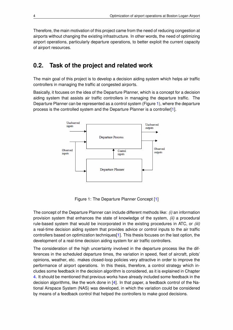
Basically, it focuses on the idea of the Departure Planner, which is a concept for a decisionaiding system that assists air traffic controllers in managing the departure traffic. TheDeparture Planner can be represented as a control system (Figure 1), where the departureprocess is the controlled system and the Departure Planner is a controller[1].
Figure 1: The Departure Planner Concept [1]
The concept of the Departure Planner can include different methods like: (i) an informationprovision system that enhances the state of knowledge of the system, (ii) a proceduralrule-based system that would be incorporated in the existing procedures in ATC, or (iii)a real-time decision aiding system that provides advice or control inputs to the air trafficcontrollers based on optimization techniques[1]. This thesis focuses on the last option, thedevelopment of a real-time decision aiding system for air traffic controllers.
The consideration of the high uncertainty involved in the departure process like the dif-ferences in the scheduled departure times, the variation in speed, fleet of aircraft, pilots’opinions, weather, etc. makes closed-loop policies very attractive in order to improve theperformance of airport operations. In this thesis, therefore, a control strategy which in-cludes some feedback in the decision algorithm is considered, as it is explained in Chapter4. It should be mentioned that previous works have already included some feedback in thedecision algorithms, like the work done in [4]. In that paper, a feedback control of the Na-tional Airspace System (NAS) was developed, in which the variation could be consideredby means of a feedback control that helped the controllers to make good decisions.

5
Also, another task of the thesis is to develop a model of the airport which can be usedto apply the control strategy proposed. In [4], a model based on aggregate flows wasalso developed, which simulate the behavior of the system as well as it is tractable for thepurpose of control. This type of models are gaining popularity nowadays due to their lotsof advantages, so in this project is decided to develop a model of this type to simulate thedynamics of the studied airport.
Finally, it is also needed to chose an airport in order to evaluate the results of the model andthe proposed control strategy. Then, the requirements for the selection of the airport arebasically two: (i) The airport has to be congested and (ii) enough data has to be availablein order to be able to build a simulation and an adequate model. Considering all this, thechosen airport is Boston Logan Airport, because it has been already studied in differentprevious works like [1, 5] and also because it has high congestion in certain periods of theday.
Actually, the work done in [5] consists on the development and field test of a strategywhich controls the rate in which pushbacks are done in order to reduce taxi-times, whichis also the purpose of this thesis. However, it did not model other interesting parts ofthe airport that should also be managed efficiently, like intersecting and merging points,runway crossings, etc., effects that are considered in this thesis.
To summarize, the tasks that have been done in this project are shown in the list below:
• Understanding of the general departure process.
• Study of the specific characteristics of Boston Logan Airport as well as collect therequired data to build a realistic model.
• Building of the model that will be used in the control strategy.
• Selection of the control strategy to be applied in the departure process.
• Simulation of the departure process at Boston Logan Airport, using the current con-trol policy in airport operations (FCFS) and the proposed strategy in this project.
• Analysis of the results.


CHAPTER 1. THE AIRPORT SYSTEM
In this section, the main components of the airport system that affect to the departureprocess are defined, as well as its interactions with the NAS.
1.1. Components of the airport system
As this project focuses on studying the departure process, it is important to know how theairport systems works and which are its main components.
The main components of the airport system are shown in Figure 1.1, which are the gates,the ramp area around the gates, the taxiways that connect the ramp (or directly the gates)with the runway and the runway system. Also, there are the entry and exit fixes, which arethe points where the aircraft enter and exit the airport system, going or coming from theNAS.
Figure 1.1: Schematic of the airport system components [2]
Basically, the process is as follows: aircraft enter to the system by an entry fix (comingfrom the NAS), they use the runways to land and, after it, they go through the taxiwaysand the ramp area in order to arrive to the gate. Once they are in the gate the turnaroundoperations take place, which means that aircraft are converted into departing aircraft.
When aircraft are ready to depart, they ask for pushback and start the departure process.They leave the gate and they move through the ramp and taxis in order to arrive to thetakeoff runway. Once there, they depart and exit the system by an exit fix.
Throughout all this process, aircraft are under the orders of ATC, another resource of theairport system as its shown in Figure 1.1. This component is of extremely importance inthe scope of this project, as it is responsible of ordering the aircraft to move or not andfollow certain paths in the airport surface. Also, it is the component that has more flexibilityto change, as it is formed by air traffic controllers and they orders can be easily modifiedin order to improve efficiency. As it has been already said, the objective of this project is to
7
8 Optimization of airport operations at Boston Logan Airport
help controllers to improve the efficiency of this orders.
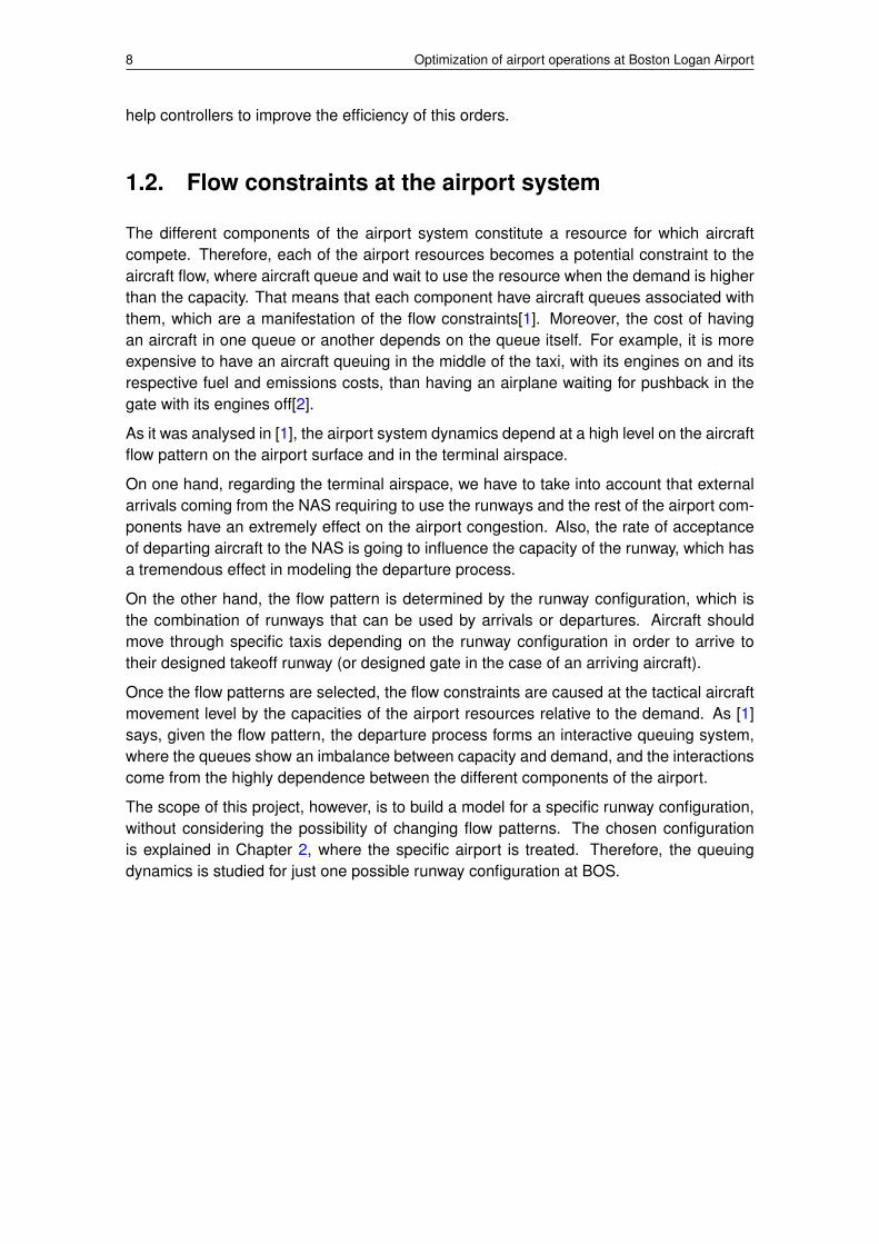
1.2. Flow constraints at the airport system
The different components of the airport system constitute a resource for which aircraftcompete. Therefore, each of the airport resources becomes a potential constraint to theaircraft flow, where aircraft queue and wait to use the resource when the demand is higherthan the capacity. That means that each component have aircraft queues associated withthem, which are a manifestation of the flow constraints[1]. Moreover, the cost of havingan aircraft in one queue or another depends on the queue itself. For example, it is moreexpensive to have an aircraft queuing in the middle of the taxi, with its engines on and itsrespective fuel and emissions costs, than having an airplane waiting for pushback in thegate with its engines off[2].
As it was analysed in [1], the airport system dynamics depend at a high level on the aircraftflow pattern on the airport surface and in the terminal airspace.
On one hand, regarding the terminal airspace, we have to take into account that externalarrivals coming from the NAS requiring to use the runways and the rest of the airport com-ponents have an extremely effect on the airport congestion. Also, the rate of acceptanceof departing aircraft to the NAS is going to influence the capacity of the runway, which hasa tremendous effect in modeling the departure process.
On the other hand, the flow pattern is determined by the runway configuration, which isthe combination of runways that can be used by arrivals or departures. Aircraft shouldmove through specific taxis depending on the runway configuration in order to arrive totheir designed takeoff runway (or designed gate in the case of an arriving aircraft).
Once the flow patterns are selected, the flow constraints are caused at the tactical aircraftmovement level by the capacities of the airport resources relative to the demand. As [1]says, given the flow pattern, the departure process forms an interactive queuing system,where the queues show an imbalance between capacity and demand, and the interactionscome from the highly dependence between the different components of the airport.
The scope of this project, however, is to build a model for a specific runway configuration,without considering the possibility of changing flow patterns. The chosen configurationis explained in Chapter 2, where the specific airport is treated. Therefore, the queuingdynamics is studied for just one possible runway configuration at BOS.

CHAPTER 2. OVERVIEW OF LOGAN AIRPORT
In this chapter, a description of the chosen runway configuration for the airport of studyand its posterior simplification is explained. Also, a dynamic queuing network to representthis configuration is designed and explained.
Firstly, I would like to briefly mention why this airport is chosen. As it is said in the intro-duction, the proposed method has the goal of dealing with congested situations in majorairports, that’s why a congested airport like BOS needs to be chosen. Moreover, the de-sire to build a model as realistic as possible requires to chose an airport which has enoughavailable data; in other words, an airport which has already been studied. These twoneeds are the main reasons why Boston Logan International Airport was chosen.
Secondly, I would like to comment that all the analysis done in this chapter are focused oncharacteristics of the airport which are relevant for the construction of the model (Chapter3), the one is used to apply the proposed control policy. Also, as this project has thegoal of doing an initial test to verify if the proposed method is able to optimize the currentoperations, the real runway configuration and operations in the airport are simplified. Thatmeans that, as we are not interested in building a large model for a first approach, thecomplexity of the studied flow pattern is not too high and so the Eulerian model that it isdeveloped in Chapter 3, which has just a small number of queues.
2.1. Choice of the runway configuration (22L, 27 / 22R,22L) and simplification
In order to adapt a congestion management strategy for an airport, it is important to identifywhich are the most common runway configurations in that airport, because it would not bereally useful to study a runway configuration which is rarely used.
In Figure 2.1, the use of the different runway configurations at BOS in the summer monthsof 2011 derived from ASDE-X data are shown [3].
Figure 2.1: BOS Runway Configuration Usage [3]
9

10 Optimization of airport operations at Boston Logan Airport
It is clear that there are two main configurations at BOS: 22L, 27 / 22R, 22L1 and 4R, 4L /9, 4R. In this thesis, the first one is chosen due to more available data.
Also, as it is said in Section 1.2., once the runway configuration is chosen, the flow patternis determined. In Figure 2.2, the flow pattern corresponding to this configuration is shown.
Figure 2.2: Flow pattern under 22L, 27 / 22R, 22L configuration [1]
In this configuration, runways 27 and 22L are the arrival runways and runways 22R and22L are used for departures. However, not all of them are used equally because each ofthem has its functionality. As it is said, this model serves to obtain a first approach, sothe runway configuration is going to be simplified taking into account which parts are moreimportant to consider.
As it is said in [1], runway 22R is the primary departure runway, while the longer 22Lrunway is only used for heavy departures. Therefore, it is considered that assign all depar-tures to runway 22R is a good approach which allow to treat runway 22L only for landings.Also, it is important to take into account that runways 22R and 22L are dependent par-allel runways (they are separated less than 2500ft), which means that specific operatingrules, as separation minims, have to be applied. This interaction is explained in more de-tail in Section 2.4.. Finally, it is desired to assign all the arrivals to one runway in order tosimplify even more the configuration. The fact of testing if the proposed model is able torepresent the interaction between dependent parallel runway is considered interesting, sofinally runway 22L is chosen as the landing runway whereas runway 27 is discarded.
1The runway configuration symbol starts with the list of arrival runways separated by commas, then aslash, then the list of departure runways separated by commas.

CHAPTER 2. OVERVIEW OF LOGAN AIRPORT 11
2.2. Interactive queuing system
As it is said, the aircraft movement in the airport system can be represented as a networkof queues, where aircraft wait to operate on the airport resources. In this section, therefore,the queuing behavior of the airport system is described in detail.
In order to do that, a figure taken from [1], which shows the queue formations on the airportsurface in configuration 22L, 27 / 22R, 22L , is shown (Figure 2.3) and explained. In orderto better understand this Figure, a color code is used to differentiate the different types ofqueues.
Figure 2.3: Queuing network under the 22L, 27 / 22R, 22L runway configuration [1]
2.2.1. Queues for the departure segment
First of all, it is really important to understand how the dynamic queuing system shownin Figure 2.3 works, which represents the departure and arrival processes in the airportsurface. Also, it is important to remember that the task of the controllers is to manage theaircraft movement over these queues in order to maintain safe operations. Some of their

12 Optimization of airport operations at Boston Logan Airport
tasks include to sequence the aircraft at merging points and intersections as well as askingfor holding if is is necessary.
The departure process starts when an aircraft is ready for pushback and the pilot asks fora clearance to the controller. At that point, the aircraft enters the pushback queue (shownin pink). In the model built in this thesis, as it is explained in chapter 3, this queue is theentrance to the airport system for all departing aircraft.
Nowadays, controllers deliver the pushback clearance to aircraft according to a First ComeFirst Served (FCFS) sequence in order to be fair with all the airlines, even if this strategy isnot the most efficient. It is extremely important to take into account this concept of fairnessin during all the project if the objective is to develop a control strategy which has to beaccepted for the airlines as well as airport operators.
Once the controllers allow a pushback, aircraft enter to the ramp queue (shown in orange)before to move to the departure taxi queues (shown in yellow), in which they move to thedeparture runway.
In the case of BOS, controllers usually assign all the departing aircraft to taxi Kilo (the outerone) and the arriving aircraft to taxi Alpha (the inner one)[1], letters K and A in Figure 2.3.Doing this, they allow to separate opposite flows as much as possible and the interactionsare much less.
After this, all departing aircraft move to taxiway November (shown with letter N) wheredifferent flows merge in order to join the takeoff queues (shown in green). In these queuesis where aircraft wait until runways 22R or 22L are available for takeoff. In this specificconfiguration, there is also a runway crossing queue for departing aircraft that need todepart in runway 22L (shown in light green). Finally, we can consider that aircraft leave theairport system once they have departed.
2.2.2. Queues for the arrival segment
In the arrival segment, we start with landing queues, where aircraft who want to land atBOS wait for availability of the runway 22L. Once they receive the clearance to land fromthe controller, they land and exit the runway for one of the exits, depending on the distancethey need to carry out the landing. In the case of study, we see that arriving aircraft needto cross the departure runway in order to get to their gates. So, as it is shown, aircraft jointhe arrival runway crossing queues after the landing.
In these queues, aircraft have to wait until the departure runway is empty and they cancross and enter the taxiway system, where they join the arrival taxi queues (light blue) andmix with departing traffic. As it is indicated in Figure 2.3, after that, aircraft taxi to the rampin order to get to the assigned gate and perform the turnaround. If the assigned gate isoccupied by another aircraft or the gate alley leading to the gate is blocked, the aircrafthave to wait and form a gate-occupied or alley blocked queue (shown in violet).
Finally, once they get to their respective gate, they perform the turnaround (white in Figure2.3) and are converted into departing aircraft.
CHAPTER 2. OVERVIEW OF LOGAN AIRPORT 13
2.3. Queuing system for the simplified model
In this section, the final simplification of the queuing system for the chosen model is ex-plained.
First of all, just remember that runway 22L has been already neglected as a departurerunway, which means that the departure runway crossing queue can be eliminated of thequeuing network.
Secondly, it is important to remember that this project focus on the departure process.Therefore, although we cannot forget about arrivals because they have high influence inthe departure process2, the model can be simplified considering only the parts of thearrival process that highly affect the departures.
For example, on one hand, it has been said that in this configuration controllers tend to as-sign all departing aircraft to taxiway Kilo and arriving ones to taxiway Alpha, which reducesinteraction. Also, [5] says that gate conflicts at BOS are relatively infrequent. Therefore,eliminating the arrival taxi and gate occupied queues in order to reduce the size of the net-work of queues is considered a good approach which will not influence too much the result.On the other hand, however, the great influence of having dependent parallel runways forthe departures and landings and the need for arrival aircraft to cross the departure runwayto get to their gates requires the consideration of these two types of queues, as they havea huge influence in the departure process.
So, to sum up, the arriving aircraft are treated from the landing queue until they havecrossed the departure runway, where they are not considered anymore because it is sup-posed that they arrive to their assigned gates without causing too much problems to thedeparting process. The only way they can interact with the departing taxiing aircraft is that,if the queue in taxiway Kilo is too big, aircraft cannot cross the departure runway in orderto move to taxiway Alpha; but this interaction is going to be treated in Section 4.2.3..
Doing this, it can be said that this model does not consider explicitly the turnaround oper-ations, as arrivals and departures are treated separately. However, as gate conflicts rarelyhappens at BOS, it is supposed that turnaround operations are done without problemsand, when aircraft are ready for pushback, they ask for clearance while they wait in thepushback queue.
Moreover, the ramp queues has also been neglected and it is supposed that after pushbackaircraft directly move to the taxis.
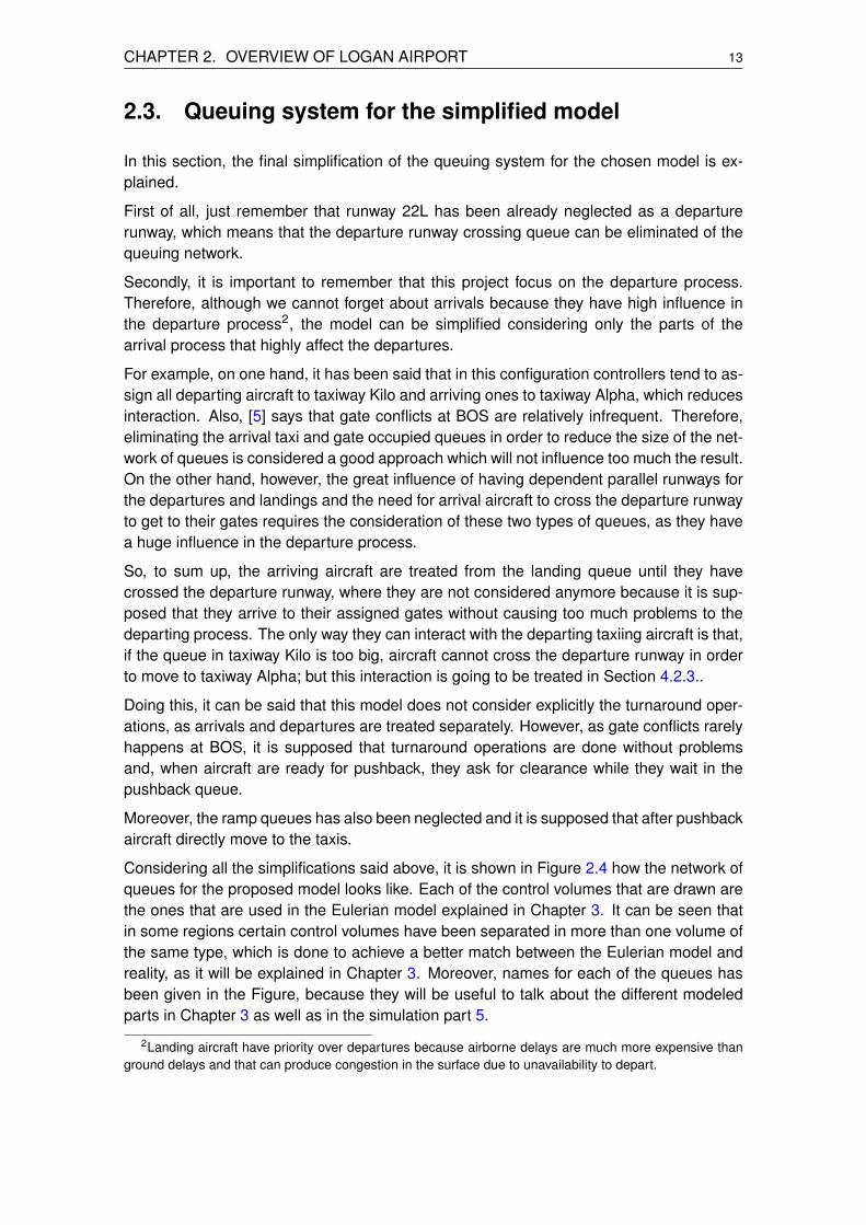
Considering all the simplifications said above, it is shown in Figure 2.4 how the network ofqueues for the proposed model looks like. Each of the control volumes that are drawn arethe ones that are used in the Eulerian model explained in Chapter 3. It can be seen thatin some regions certain control volumes have been separated in more than one volume ofthe same type, which is done to achieve a better match between the Eulerian model andreality, as it will be explained in Chapter 3. Moreover, names for each of the queues hasbeen given in the Figure, because they will be useful to talk about the different modeledparts in Chapter 3 as well as in the simulation part 5.
2Landing aircraft have priority over departures because airborne delays are much more expensive thanground delays and that can produce congestion in the surface due to unavailability to depart.
14 Optimization of airport operations at Boston Logan Airport
Figure 2.4: Queuing network for our model, adapted from [1] for the 22L, 27 / 22R, 22Lconfiguration
The flow pattern resulting from the runway configuration simplified it is also shown in Figure2.5. We can easily see how arrival aircraft interact with departing taxing aircraft just afterthey have crossed the runway 22R, however, we can also see that after that, they do nothave any other important interaction.
Figure 2.5: Flow pattern in our configuration, adapted from [1] for 22L, 27 / 22R, 22Lconfiguration
CHAPTER 2. OVERVIEW OF LOGAN AIRPORT 15
Finally, I would like to summarize all the hypothesis and simplifications that have beenconsidered in this chapter in the following list:
• Runway 22L is only for arrivals.
• Runway 27 is not considered.
• Turnaround operation are supposed to be done without problems.
• Taxi queues for arrivals are not considered
• After pushback, aircraft directly move to taxi queues, which means that ramp queuesare not considered.
• As gate conflicts rarely happens, gate occupied queues are neglected.
• Only two runway crossing queues are considered, as only an idea of their effect onthe system is required.
• Missed approaches are not considered.
• Possible failures when an aircraft is already taking off is not considered. Once theyhave left the gate, they move until the departure runway if there are not other aircraftwhich are blocking the path.
• Downstream queues in the exit fixes are not considered. Therefore, once an aircrafthave left the runway queue, it leaves the airport system.
2.4. Characterization of our model
In this section, some important data of Boston Logan Airport is shown. This information iscompletely necessary in order to model the airport, as certain values need to be consid-ered to achieve a realistic model. This section includes data regarding regulations, airportdimensions, typical speeds, etc.
2.4.1. Taxi times and minimum separation
To model the taxiways of BOS, it is necessary to know which are the unimpeded taxi times,the regulations that have to be applied in the taxi (like the minimum separation betweenaircraft) as well as which are the typical velocities in the process of taxiing.
First of all, it is interesting to get some information about the unimpeded taxi times at BOS,as it is really important to have some realistic data to compare the obtained results andbe able to evaluate the degree of reliability of the simulations. By using data from theAviation System Performance Metrics (ASPM) database [6] and from [5, 7], an estimationof the unimpeded taxi-out time for aircraft coming from each of the terminals is computed.However, it is really important to take into account that this data is just an approximation,as the data analysed does not consider all the simplifications that have been done in this
16 Optimization of airport operations at Boston Logan Airport
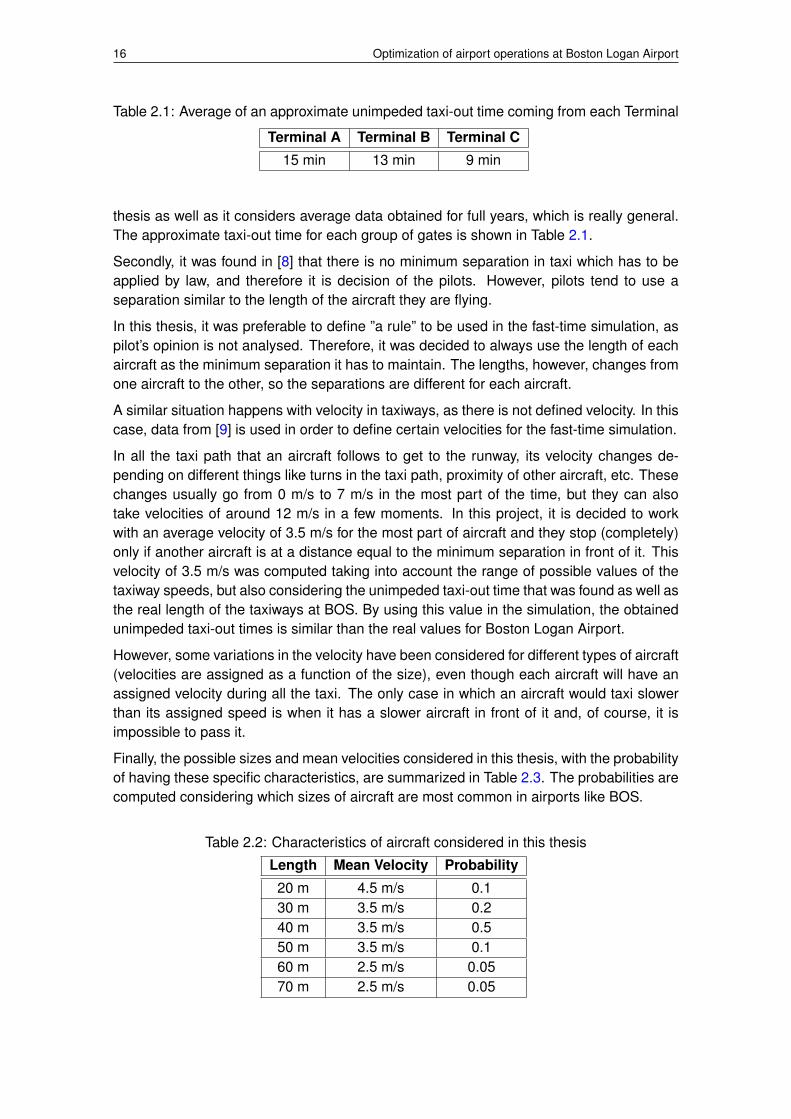
Table 2.1: Average of an approximate unimpeded taxi-out time coming from each Terminal
Terminal A Terminal B Terminal C
15 min 13 min 9 min
thesis as well as it considers average data obtained for full years, which is really general.The approximate taxi-out time for each group of gates is shown in Table 2.1.
Secondly, it was found in [8] that there is no minimum separation in taxi which has to beapplied by law, and therefore it is decision of the pilots. However, pilots tend to use aseparation similar to the length of the aircraft they are flying.
In this thesis, it was preferable to define ”a rule” to be used in the fast-time simulation, aspilot’s opinion is not analysed. Therefore, it was decided to always use the length of eachaircraft as the minimum separation it has to maintain. The lengths, however, changes fromone aircraft to the other, so the separations are different for each aircraft.
A similar situation happens with velocity in taxiways, as there is not defined velocity. In thiscase, data from [9] is used in order to define certain velocities for the fast-time simulation.
In all the taxi path that an aircraft follows to get to the runway, its velocity changes de-pending on different things like turns in the taxi path, proximity of other aircraft, etc. Thesechanges usually go from 0 m/s to 7 m/s in the most part of the time, but they can alsotake velocities of around 12 m/s in a few moments. In this project, it is decided to workwith an average velocity of 3.5 m/s for the most part of aircraft and they stop (completely)only if another aircraft is at a distance equal to the minimum separation in front of it. Thisvelocity of 3.5 m/s was computed taking into account the range of possible values of thetaxiway speeds, but also considering the unimpeded taxi-out time that was found as well asthe real length of the taxiways at BOS. By using this value in the simulation, the obtainedunimpeded taxi-out times is similar than the real values for Boston Logan Airport.
However, some variations in the velocity have been considered for different types of aircraft(velocities are assigned as a function of the size), even though each aircraft will have anassigned velocity during all the taxi. The only case in which an aircraft would taxi slowerthan its assigned speed is when it has a slower aircraft in front of it and, of course, it isimpossible to pass it.
Finally, the possible sizes and mean velocities considered in this thesis, with the probabilityof having these specific characteristics, are summarized in Table 2.3. The probabilities arecomputed considering which sizes of aircraft are most common in airports like BOS.
Table 2.2: Characteristics of aircraft considered in this thesis
Length Mean Velocity Probability
20 m 4.5 m/s 0.130 m 3.5 m/s 0.240 m 3.5 m/s 0.550 m 3.5 m/s 0.160 m 2.5 m/s 0.0570 m 2.5 m/s 0.05
CHAPTER 2. OVERVIEW OF LOGAN AIRPORT 17
Finally, regarding the minimum separation and the considered velocities, the maximumthroughput of each of the control volumes that represent a part of the taxiway is computed.In order to do it, the most common values for velocities and sizes are used, as it is notpossible to know how many aircraft of each type there will be at a certain control volume ateach time. Therefore, it is preferred to consider a constant maximum throughput computedwith the mean values. By using a speed of 3.5 m/s, a separation of 40 m and an aircraftsize of 40 m, the maximum throughput from a taxiway control volume in one minute givesa result of 3 acc/min.
2.4.2. Interaction between arrivals, departures and runway crossingqueues
Another important thing to consider in order to model the airport are the regulations thatapply to arrivals and departures.
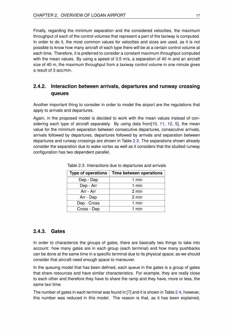
Again, in the proposed model is decided to work with the mean values instead of con-sidering each type of aircraft separately. By using data from[10, 11, 12, 5], the meanvalue for the minimum separation between consecutive departures, consecutive arrivals,arrivals followed by departures, departures followed by arrivals and separation betweendepartures and runway crossings are shown in Table 2.3. The separations shown alreadyconsider the separation due to wake vortex as well as it considers that the studied runwayconfiguration has two dependent parallel.
Table 2.3: Interactions due to departures and arrivals
Type of operations Time between operations
Dep - Dep 1 minDep - Arr 1 minArr - Arr 2 minArr - Dep 2 min
Dep - Cross 1 minCross - Dep 1 min
2.4.3. Gates
In order to characterize the groups of gates, there are basically two things to take intoaccount: how many gates are in each group (each terminal) and how many pushbackscan be done at the same time in a specific terminal due to its physical space; as we shouldconsider that aircraft need enough space to maneuver.
In the queuing model that has been defined, each queue in the gates is a group of gatesthat share resources and have similar characteristics. For example, they are really closeto each other and therefore they have to share the ramp and they have, more or less, thesame taxi time.
The number of gates in each terminal was found in [7] and it is shown in Table 2.4, however,this number was reduced in this model. The reason is that, as it has been explained,

18 Optimization of airport operations at Boston Logan Airport
turnaround operations are not explicitly considered, however, it should be considered thatsome gates should be reserved for these kind of operations.
Finally, considering data from [1], it was considered reasonable to allow a maximum of twopushbacks in each terminal at each minute.
Table 2.4: Number of gates in reality and in the model
Terminal Real number of gates Considered number of gates
A 15 10B 38 25C 24 16
CHAPTER 3. EULERIAN MODEL OF LOGANAIRPORT
In this section, I propose an Eulerian Model of Boston Logan Airport (BOS) that allowsdifferent control approaches, based on the model developed in [4] to represent the NationalAirspace System (NAS) dynamics. However, this time the model will be used to representthe dynamics of the departure process at BOS, although it could be used to represent anyairport by modeling adequately the corresponding data.
Eulerian models are control volume based, which means that the important thing is tocontrol the aircraft counts in certain control volumes instead of following individual aircraft(Lagrangian models). Nowadays, models based on control volumes are preferred in TrafficFlow Management improvement techniques basically for two reasons: (i) They are compu-tationally tractable, and their computational complexity does not depend on the number ofaircraft, but only on the size of the physical problem of interest. (ii) Their control theoreticstructure enables the use of standard methodologies to analyse them[13].
As it is done in [4], I start by deciding the points where the traffic flow needs to be controlled,which will correspond with the boundaries of the control volumes. So, it seems clear thata good approach is to use as a control volumes the different queues that I have describedin section 2.3., where aircraft wait to operate on airport resources such as gate, ramp,taxiways and runways. The controls of my model, therefore, correspond to give or notaccess to certain airport resource.
However, there are some important features that I have to take into account in modelingthe airport surface instead of the airspace of the NAS as it is done in [4]: (i) Paths to followare fixed as well as their distance is constant, (ii) just one airplane fits in width in a taxi (anaircraft cannot pass another one) and (iii) aircraft velocity in taxi cannot have big changes(so the unimpeded time to cross a control volume cannot be decreased).
Considering this, we can think that having big control volumes in the airport surface canproduce high uncertainty in knowing where the aircraft is placed inside the volume. Forexample, if we have a part of the taxi that needs approximately 6 minutes to be crossed(as Taxi B) and we want to compute the aircraft counts each minute (discretization time),we cannot know if the aircraft has just entered the control volume and consequently stillneeds 5 minutes to cross all the volume or if this aircraft is going to exit the volume in thenext minute.
That means that different control volumes should have similar dimensions and the timerequired to cross them should be coherent with the discretization time of the dynamic sys-tem. Adding control volumes increase precision, because the knowledge about the airportsurface is more accurate, as well as provides more decision support. However, increasingthe number of volumes makes the system bigger, which means that computational costincreases (the number of states increases) and flexibility to adapt decreases, because Ihave to consider that I have to be able to count the number of aircraft in each volume inrelatively small periods of time. Therefore, a balance between size of the control volumesand number of queues in the system is required, because having a high number of statescan produce lots of problems when trying to solve the system in attempts to find optimalcontrols.
19
20 Optimization of airport operations at Boston Logan Airport
In section 2.4. the unimpeded time to pass through each control volume was analysed.Considering all that was said, it was supposed that a good time-discretization could be1 minute (T=1min), as it is the time between consecutive departures, which is a goodreference, and also it is small enough to avoid that aircraft can enter and leave the controlvolume in the same period. So, in the following sections all the numbers will be adapted tothis time-discretization. Also, this number determines the time between each decision ofthe controllers, which means that they have to give instructions to the pilots of the aircraftevery minute.
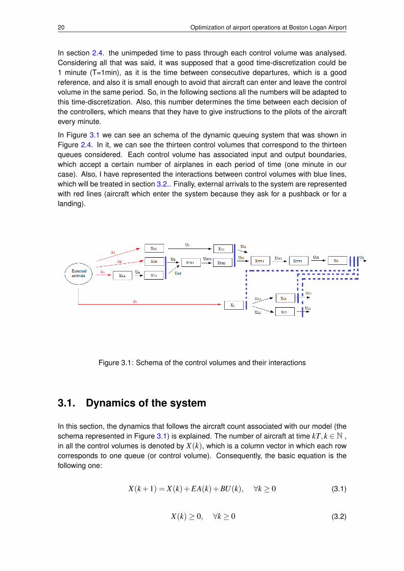
In Figure 3.1 we can see an schema of the dynamic queuing system that was shown inFigure 2.4. In it, we can see the thirteen control volumes that correspond to the thirteenqueues considered. Each control volume has associated input and output boundaries,which accept a certain number of airplanes in each period of time (one minute in ourcase). Also, I have represented the interactions between control volumes with blue lines,which will be treated in section 3.2.. Finally, external arrivals to the system are representedwith red lines (aircraft which enter the system because they ask for a pushback or for alanding).
Figure 3.1: Schema of the control volumes and their interactions
3.1. Dynamics of the system
In this section, the dynamics that follows the aircraft count associated with our model (theschema represented in Figure 3.1) is explained. The number of aircraft at time kT,k ∈ N ,in all the control volumes is denoted by X(k), which is a column vector in which each rowcorresponds to one queue (or control volume). Consequently, the basic equation is thefollowing one:
X(k+1) = X(k)+EA(k)+BU(k), ∀k ≥ 0 (3.1)
X(k)≥ 0, ∀k ≥ 0 (3.2)
CHAPTER 3. EULERIAN MODEL OF LOGAN AIRPORT 21
U(k)≥ 0, ∀k ≥ 0 (3.3)
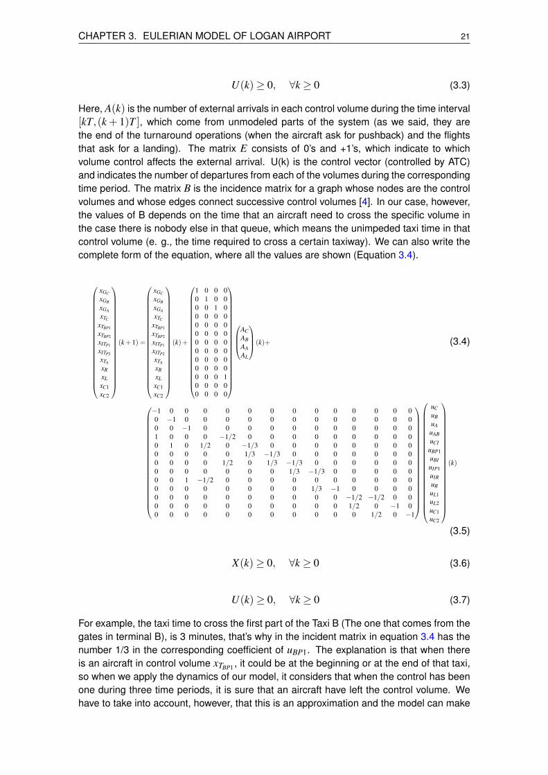
Here, A(k) is the number of external arrivals in each control volume during the time interval[kT,(k + 1)T ], which come from unmodeled parts of the system (as we said, they arethe end of the turnaround operations (when the aircraft ask for pushback) and the flightsthat ask for a landing). The matrix E consists of 0’s and +1’s, which indicate to whichvolume control affects the external arrival. U(k) is the control vector (controlled by ATC)and indicates the number of departures from each of the volumes during the correspondingtime period. The matrix B is the incidence matrix for a graph whose nodes are the controlvolumes and whose edges connect successive control volumes [4]. In our case, however,the values of B depends on the time that an aircraft need to cross the specific volume inthe case there is nobody else in that queue, which means the unimpeded taxi time in thatcontrol volume (e. g., the time required to cross a certain taxiway). We can also write thecomplete form of the equation, where all the values are shown (Equation 3.4).
xGC
xGB
xGA
xTC
xTBP1
xTBP2
xITP1
xITP2
xTA
xRxLxC1xC2
(k+1) =
xGC
xGB
xGA
xTC
xTBP1
xTBP2
xITP1
xITP2
xTA
xRxLxC1xC2
(k)+
1 0 0 00 1 0 00 0 1 00 0 0 00 0 0 00 0 0 00 0 0 00 0 0 00 0 0 00 0 0 00 0 0 10 0 0 00 0 0 0
ACABAAAL
(k)+ (3.4)
−1 0 0 0 0 0 0 0 0 0 0 0 0 00 −1 0 0 0 0 0 0 0 0 0 0 0 00 0 −1 0 0 0 0 0 0 0 0 0 0 01 0 0 0 −1/2 0 0 0 0 0 0 0 0 00 1 0 1/2 0 −1/3 0 0 0 0 0 0 0 00 0 0 0 0 1/3 −1/3 0 0 0 0 0 0 00 0 0 0 1/2 0 1/3 −1/3 0 0 0 0 0 00 0 0 0 0 0 0 1/3 −1/3 0 0 0 0 00 0 1 −1/2 0 0 0 0 0 0 0 0 0 00 0 0 0 0 0 0 0 1/3 −1 0 0 0 00 0 0 0 0 0 0 0 0 0 −1/2 −1/2 0 00 0 0 0 0 0 0 0 0 0 1/2 0 −1 00 0 0 0 0 0 0 0 0 0 0 1/2 0 −1
uCuBuAuABuCI
uBP1uBIuIP1uIRuRuL1uL2uC1uC2
(k)
(3.5)
X(k)≥ 0, ∀k ≥ 0 (3.6)
U(k)≥ 0, ∀k ≥ 0 (3.7)
For example, the taxi time to cross the first part of the Taxi B (The one that comes from thegates in terminal B), is 3 minutes, that’s why in the incident matrix in equation 3.4 has thenumber 1/3 in the corresponding coefficient of uBP1. The explanation is that when thereis an aircraft in control volume xTBP1 , it could be at the beginning or at the end of that taxi,so when we apply the dynamics of our model, it considers that when the control has beenone during three time periods, it is sure that an aircraft have left the control volume. Wehave to take into account, however, that this is an approximation and the model can make
22 Optimization of airport operations at Boston Logan Airport
mistakes due to the uncertainty caused by the size of the control volume. For all the othernumbers the explanation is the same, if the unimpeded time cross the control volume is 2minutes, the coefficient in matrix B will be 1/2, and if it is 1 minute the coefficient will be1. Also, depending if the control affects the the entering aircraft to a control volume or thedeparting ones, that number will be positive or negative.
Finally, we can also see that there are non-negativity constraints, because clearly thenumber of aircraft in a control volume cannot be negative as well as the number of aircraftwhich depart from a control volume.
3.2. Restrictions and interactions
In this section, all the restrictions as maximum throughput, maximum capacity and interac-tions between different volumes of the system are explained. The equation that models thedynamics of the system (3.1) is the basic equation of the model, however, this dynamics isrestricted for different physical factors that need to be taken into account.
3.2.1. Maximum throughput
First of all, we need to know which is the maximum throughput in each control volume,which means the maximum number of departures accepted in each volume.
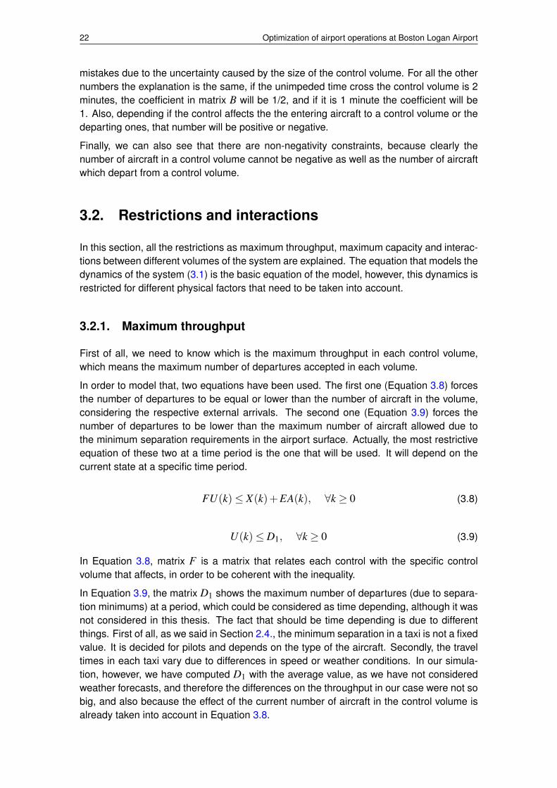
In order to model that, two equations have been used. The first one (Equation 3.8) forcesthe number of departures to be equal or lower than the number of aircraft in the volume,considering the respective external arrivals. The second one (Equation 3.9) forces thenumber of departures to be lower than the maximum number of aircraft allowed due tothe minimum separation requirements in the airport surface. Actually, the most restrictiveequation of these two at a time period is the one that will be used. It will depend on thecurrent state at a specific time period.
FU(k)≤ X(k)+EA(k), ∀k ≥ 0 (3.8)
U(k)≤ D1, ∀k ≥ 0 (3.9)
In Equation 3.8, matrix F is a matrix that relates each control with the specific controlvolume that affects, in order to be coherent with the inequality.
In Equation 3.9, the matrix D1 shows the maximum number of departures (due to separa-tion minimums) at a period, which could be considered as time depending, although it wasnot considered in this thesis. The fact that should be time depending is due to differentthings. First of all, as we said in Section 2.4., the minimum separation in a taxi is not a fixedvalue. It is decided for pilots and depends on the type of the aircraft. Secondly, the traveltimes in each taxi vary due to differences in speed or weather conditions. In our simula-tion, however, we have computed D1 with the average value, as we have not consideredweather forecasts, and therefore the differences on the throughput in our case were not sobig, and also because the effect of the current number of aircraft in the control volume isalready taken into account in Equation 3.8.

CHAPTER 3. EULERIAN MODEL OF LOGAN AIRPORT 23
We can also expand both matrices considering all that was said in section 2.4., regardingminimum separation between airplanes in the taxis, the physical space at the ramp in orderto carry out the pushbacks, the minimum time between consecutive departures or arrivals,etc. The expanded matrices of all the restrictions are shown in Appendix A.
3.2.2. Interactions between control Volumes
In this section the interactions between control volumes due to merging flows, dependentparallel runways and runway crossing queues are modeled.
On one hand, we have the interactions in the taxiways that are shown in Figure 3.1. Forexample, it is shown that aircraft coming from the volumes XTC and XT B2 merge in thevolume XIT P1, which means that the output boundary of the first two volumes coincideswith the input boundary of the last one. In the previous section, we have analysed themaximum throughput of each volume independently, however, in this case we have totake into account the the flow coming from XTC and XT B2 have to be accepted for XIT P1.That means that increasing the departures from one control volume forces to reduce thedepartures of the other one. Therefore, an extra restriction is required, that could bemodeled as follows:
uCI(k)+uBI ≤ r1, ∀k ≥ 0 (3.10)
In Equation 3.10, uCI(k) represents the number of aircraft departing from XTC, uBI theones coming from XT B2 and r1 the maximum number of aircraft that can enter in volumeXIT P1 in a specific period.
On the other hand, we have all the restrictions that affect the departure runway. Firstly, aswe have seen in Section 2.4., there is a required minimum separation between departureand arrivals due to the creation of flow vortexes. Secondly, there is an interaction betweenthe runway crossing queues and the departures, as the runway need to be clear of aircraftin order to allow a runway crossing.
Finally, the equation used to model these interactions is the following one:
CU(k)≤ R, ∀k ≥ 0 (3.11)
Here, C is a matrix which relates the controls that interact, U(k) is a column vector withall the control in the system and R is a column vector with the maximum value accepted ineach interaction. Again, the expanded matrix is shown in the Appendix A.
Also, matrix R could be time depending, because the interactions between arrivals anddepartures, for example, depend on the weather forecast, the type of aircraft, etc. In ourmodel, however, we have considered a mean value, without considering big changes inthe weather.
3.2.3. Capacity of the queues
The big difference between modeling the airport surface instead of the airspace, as in [4],is that the airport has a much more limited physical space. In other words, the number of

24 Optimization of airport operations at Boston Logan Airport
aircraft that fit in the pushback queues is determined by the number of gates in the airport,the number or aircraft in a certain taxiway also depends in the length of it, etc. Therefore,capacity limits in each control volume are considered.
This constraint is represented as follows:
X(k)≤ S, ∀k ≥ 0 (3.12)
where S is a column vector which contains the maximum capacity of each queue. Again,the expanded equation is shown in Appendix A.
3.3. Summary of the model
Finally, this section is just to join all the equations of the model, dynamics and restrictions,that have been explained in the previous two sections. The purpose of represent all theequations together here is that, in all the following chapters, will be extremely useful tohave all this information easily accessible, as it is a key part in all of them.
So finally, our model is represented by:
X(k+1) = X(k)+EA(k)+BU(k), ∀k ≥ 0 (3.13)
FU(k)≤ X(k)+EA(k), ∀k ≥ 0 (3.14)
U(k)≤ D1, ∀k ≥ 0 (3.15)
CU(k)≤ R, ∀k ≥ 0 (3.16)
X(k)≤ S, ∀k ≥ 0 (3.17)
X(k)≥ 0, ∀k ≥ 0 (3.18)
U(k)≥ 0, ∀k ≥ 0 (3.19)

CHAPTER 4. CONTROL STRATEGIES
In this chapter, two control strategies are explained. The first one is the strategy usednowadays for air traffic controllers, which is the well-known First Come, First Served(FCFS) policy. The second one is the control strategy proposed in this thesis in orderto improve the efficiency of airport operations, which is based in Model Predictive Control(MPC).
These strategies have been used in a fast time simulation in order to analyse their effect inairport management. This simulation will help us to evaluate the performance of the pro-posed method (which uses the Eulerian Model built in Chapter 3 with an MPC approach)and compare it with the current FCFS policy.
4.1. First Come, First Served Policy
First-come, first-served (FCFS) is a service policy whereby the requests of customers (inour case aircraft) are attended to in the order that they arrived to the queues (in our casethe airport resources). Nowadays, this is the policy used for air traffic controllers, becauseit is known as the fair queue discipline[14], and that is something so important to have theacceptance of the airlines.
This policy, although it is possibly one of the fairest ones for the airlines, is clearly not theoptimal. It does not allow congestion control (like feedback mechanisms) as well as it doesnot consider the different cost of waiting in different queues [4], like the difference of waitingin the gate with the engines off or in the runway queue with the engines on. Basically, inthis policy aircraft are moved forward once they are ready to move. For example, if anaircraft is ready for pushback, it will obtain a clearance to move to the departure runwayas soon as possible even if there is a big queue in the takeoff runway.
However, the good points of this policy are that does not require a lot of information tobe applied, it is easy to implement by air traffic controllers and it usually works fine undernominal conditions.
In order to compute this strategy in the fast simulation, the use of the Eulerian Model thathas been built is not necessary, because information about each one of the queues is notrequired. Therefore, in order to implement it, what is done is to suppose that the aircraft arealways going to move forward, except when they cannot move because there is anotherairplane in front of it and the minimum separation would be violated or if the flow vortexlegislation does not allow it. In other words, the only case in which they will not moveforward is for safety restrictions.
4.2. Model Predictive Control
4.2.1. Definition of MPC
First of all, it is important to define what Model Predictive Control (MPC) exactly is. As it isdescribed in [15], MPC is a form of control in which the current control action is obtained
25

26 Optimization of airport operations at Boston Logan Airport
by solving on-line, at each sampling instant, a finite-horizon open-loop optimal controlproblem, using a dynamic model of the system to predict its future behavior as well as thecurrent state of the plant as the initial state. The result of the optimization yields an optimalcontrol sequence and the first control in this sequence is the one that will be applied to theplant.
As the future behavior of the system depends on the actions (controls) applied through thefinite-horizon, these are the variables with respect the ones we will optimize our objective[16].As it is been said, the application of these actions give us an open loop, which does nottake into account the variation of our system. However, MPC allows us to decrease theeffect of the variation by incorporating a feedback; which allows to recalculate the controlsat each sampling period considering the current state and, therefore, the variation that hasoccurred between the predicted state and the actual state.
Usually, MPC is a general tool which gives good results in constrained systems with vari-ation like the one we have (3.13-3.19) [4]. It is true that it has higher implementation andinformation requirements respect the current methods, but we have to take into accountthat we are working with a system that has a lot of uncertainty and MPC is a better ap-proach for that.
4.2.2. Formulation
In this section, the procedure to obtain a feedback control law for our system is explained.
First of all, a finite-time horizon K ≥ 0 is fixed, which in our case is 25 sampling periods,which is equivalent to 25 minutes (as T=1min). In order to choose the time horizon, themost important thing that is taken into account is the unimpeded taxi time in the airportof study. Basically, the only constraint I have is to consider a time horizon which is higherthan the unimpeded taxi time, as I want a control system able to calculate which is the bestmoment for an aircraft to leave the gate in order to arrive at the runway threshold at the bestmoment (a time when there is not too much queue, but without having an empty runwayqueue in order to profit the maximum throughput). At BOS, the longest unimpeded taxi-time is 15 minutes, which is for aircraft coming from Terminal A. From here, we proceed toincrease the horizon until better results are obtained, but taking all the time into accountthat we need a control able to solve the optimization in a few seconds, as an update isrequired each minute. Finally, in our case was found that horizons higher than 25 minutesdo not give better performance and they just slow the computation.
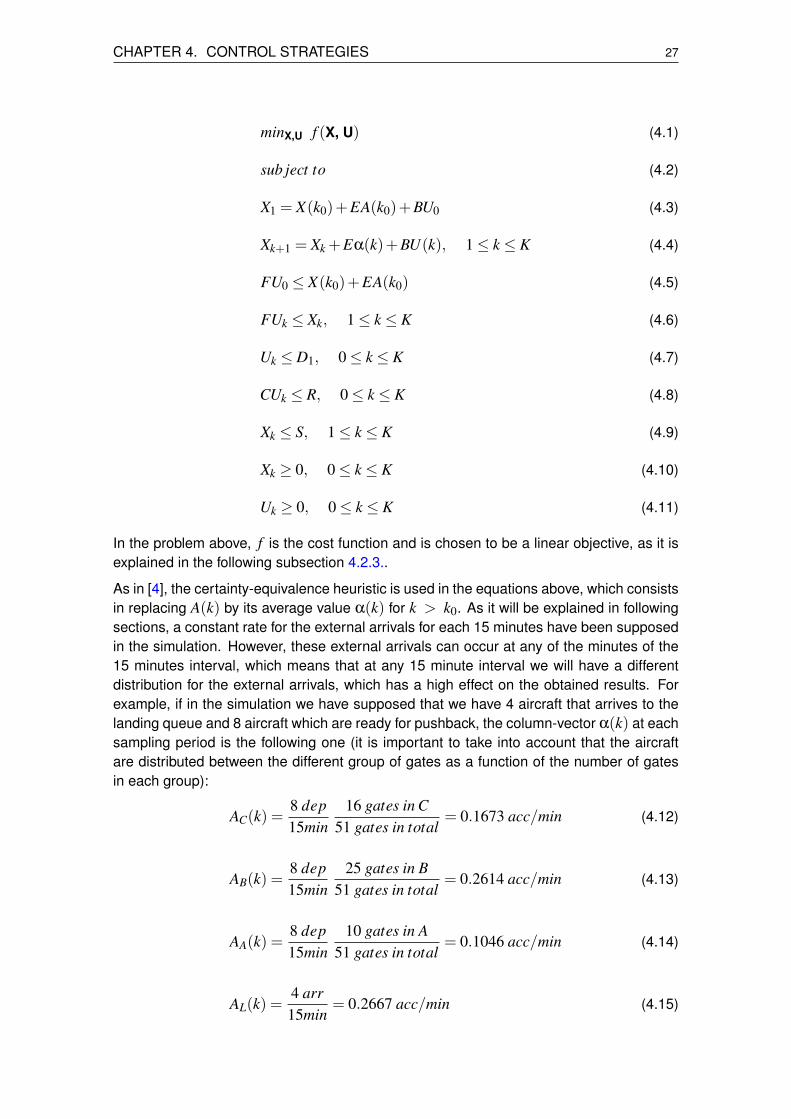
Secondly, in order to apply the MPC, it is necessary to observe, at period k0, the currentstate X(k0) in all the control volumes and the number of external arrivals A(k0). After it,we determine the controls for the current period U(k0) by solving the following problemwith variables X ={Xk}1≤k≤K+1,U ={Uk}0≤k≤K :
CHAPTER 4. CONTROL STRATEGIES 27
minX,U f (X, U) (4.1)
sub ject to (4.2)
X1 = X(k0)+EA(k0)+BU0 (4.3)
Xk+1 = Xk +Eα(k)+BU(k), 1≤ k ≤ K (4.4)
FU0 ≤ X(k0)+EA(k0) (4.5)
FUk ≤ Xk, 1≤ k ≤ K (4.6)
Uk ≤ D1, 0≤ k ≤ K (4.7)
CUk ≤ R, 0≤ k ≤ K (4.8)
Xk ≤ S, 1≤ k ≤ K (4.9)
Xk ≥ 0, 0≤ k ≤ K (4.10)
Uk ≥ 0, 0≤ k ≤ K (4.11)
In the problem above, f is the cost function and is chosen to be a linear objective, as it isexplained in the following subsection 4.2.3..
As in [4], the certainty-equivalence heuristic is used in the equations above, which consistsin replacing A(k) by its average value α(k) for k > k0. As it will be explained in followingsections, a constant rate for the external arrivals for each 15 minutes have been supposedin the simulation. However, these external arrivals can occur at any of the minutes of the15 minutes interval, which means that at any 15 minute interval we will have a differentdistribution for the external arrivals, which has a high effect on the obtained results. Forexample, if in the simulation we have supposed that we have 4 aircraft that arrives to thelanding queue and 8 aircraft which are ready for pushback, the column-vector α(k) at eachsampling period is the following one (it is important to take into account that the aircraftare distributed between the different group of gates as a function of the number of gatesin each group):
AC(k) =8 dep15min
16 gates in C51 gates in total
= 0.1673 acc/min (4.12)
AB(k) =8 dep15min
25 gates in B51 gates in total
= 0.2614 acc/min (4.13)
AA(k) =8 dep15min
10 gates in A51 gates in total
= 0.1046 acc/min (4.14)
AL(k) =4 arr15min
= 0.2667 acc/min (4.15)

28 Optimization of airport operations at Boston Logan Airport
Where the numbers 16, 25 and 10 are the number of gates that have been considered ineach terminal for our simulation as it has been said in section 2.4.3..
4.2.3. Cost function
In this section, the chosen cost function is explained in detail in order to show which is thedifferent cost of having aircraft in each queue as well as to explain which are the effectsthat are considered totally undesired.
First of all, as it has been said in the previous subsection, the objective function has beenchosen to be linear or, at least, piecewise linear in order to be able to apply the optimizationmethods used in this thesis. Secondly, just remember that the cost function shown hereis just an example of a possible objective, but it can be changed in order to adjust theimportance of each queue and the negative effects as it is desired for the designer of thecontroller.
The chosen objective is the following one:
f (X, U) :=K
∑k=1
(σ Xk +L(4− xRk)++M(xC1k−5)++M(xC2k−5)++ (4.16)
+H(xT BP1k−7)+)+K
∑k=0
G(1− (uRk +uL1k +uL2k))+
Where σ is a vector of 13 elements which contains the weighting for each queue andM,H,L and G are scalars which add a cost for undesired situations as will be explained.
Therefore, it is possible to separate the function in two parts in order to explain betterits functionality: (i) one part which gives a cost of having aircraft in the different queues,containing the term of the vector σ multiplied by the states and (ii) one part to penalizeundesired effects to help the controller to manage certain situations in this specific airport.
The first part is quite simple, it just gives different weights depending on the part of theairport system involved: having aircraft taxiing (with the engine on), having aircraft in thegate waiting for pushback (with the engine off but ready for departure), having an aircraftin the landing queue (with the engine on and in the air, which is always more expensive),etc.
In the second part four different undesired situations are considered. The first one (termwith the L) adds a cost for having less than 4 aircraft in the runway queue. Actually, thiseffect should be undesired only if the queue is empty, however, it was seen in differentsimulations that putting a one instead of a four gives empty queues lots of times due tothe uncertainty of our system. Therefore, it was preferred to increase this margin even ifthe aircraft have to do a little bit of queue before departure, as losing performance in therunway throughput was considered worse than having a queue a little bit smaller.
The second penalization(term with the M) considers the fact of having crossing queueswith more than 5 aircraft. As it is shown in figure 2.4, the length of the taxiways wherethere are the runway crossing queues are really small, and it was found that they cancontain a maximum of approximately 5 aircraft each one. If the aircraft start to accumulatein this part of the taxiway, what is going to happen is that they will cross the runway 22L
CHAPTER 4. CONTROL STRATEGIES 29
and, therefore, the arrival aircraft will not be able to land and will start to accumulate in theair, which is totally undesired.
The third one (term with the H) considers the fact of having more than 7 aircraft in the partof the taxiway K that goes from the intersection between aircraft coming from terminals Band C until the part of the taxiway that is in front of the crossing queues. Here, what isconsidered is that if there is a high congestion in this part of the airport, the aircraft in thecrossing queues cannot move until taxiway A, which is the inner taxiway designed for thearrival aircraft. Therefore, aircraft will start to accumulate in crossing queues, which thenegative effect that this cause.
Finally, the effect of exploiting the capacity envelope of the airport as much as possible isconsidered. It means that the runway utilization have to be maintained all the time, eitherfor departures or arrivals. Therefore, it was considered that one of the controls allowing adeparture or an arrival have to be active at every minute. The only exception to this ruleis having all the controls equal to zero due to safety reasons. For example, if an aircraft isallowed to land, it will need two minutes and, therefore, we will have all the controls equalsto 0 at the beginning of the second minute.
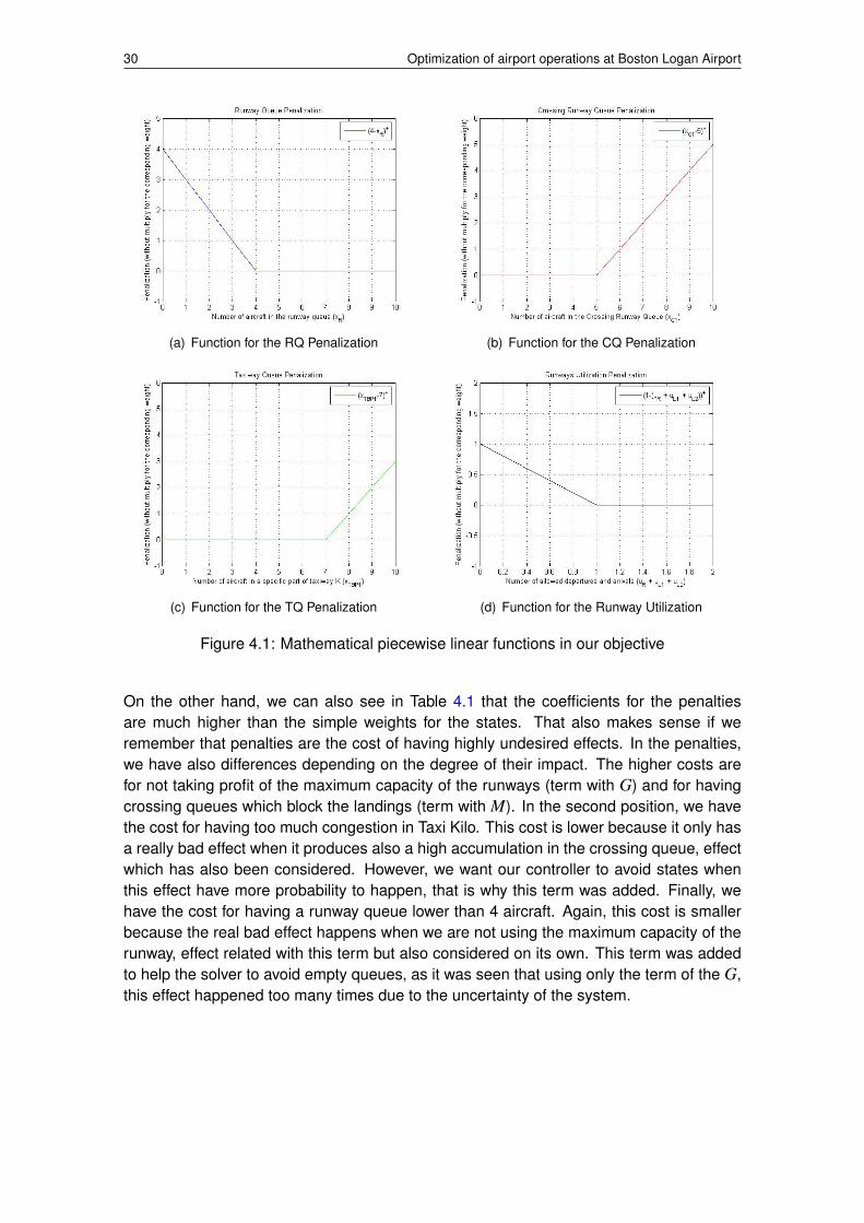
Figure 4.1 shows the piecewise linear form of the four different penalties that I have justmentioned, but without considering the scalar number that should multiply it, as my goal isjust to show its behavior. Also, the penalization for the crossing queues is shown just forone of them, as they are exactly equal.
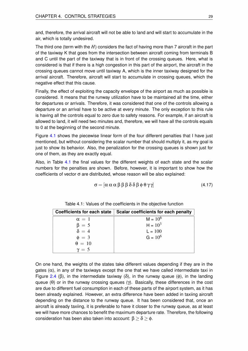
Also, in Table 4.1 the final values for the different weights of each state and the scalarnumbers for the penalties are shown. Before, however, it is important to show how thecoefficients of vector σ are distributed, whose reason will be also explained:
σ = [α α α β β β δ δ β φ θ γ γ] (4.17)
Table 4.1: Values of the coefficients in the objective function
Coefficients for each state Scalar coefficients for each penalty
α = 1 M = 106
β = 5 H = 103
δ = 4 L = 100φ = 3 G = 106
θ = 10γ = 5
On one hand, the weights of the states take different values depending if they are in thegates (α), in any of the taxiways except the one that we have called intermediate taxi inFigure 2.4 (β), in the intermediate taxiway (δ), in the runway queue (φ), in the landingqueue (θ) or in the runway crossing queues (γ). Basically, these differences in the costare due to different fuel consumption in each of these parts of the airport system, as it hasbeen already explained. However, an extra difference have been added in taxiing aircraftdepending on the distance to the runway queue. It has been considered that, once anaircraft is already taxiing, it is preferable to have it closer to the runway queue, as at leastwe will have more chances to benefit the maximum departure rate. Therefore, the followingconsideration has been also taken into account: β≥ δ≥ φ.
30 Optimization of airport operations at Boston Logan Airport
(a) Function for the RQ Penalization (b) Function for the CQ Penalization
(c) Function for the TQ Penalization (d) Function for the Runway Utilization
Figure 4.1: Mathematical piecewise linear functions in our objective
On the other hand, we can also see in Table 4.1 that the coefficients for the penaltiesare much higher than the simple weights for the states. That also makes sense if weremember that penalties are the cost of having highly undesired effects. In the penalties,we have also differences depending on the degree of their impact. The higher costs arefor not taking profit of the maximum capacity of the runways (term with G) and for havingcrossing queues which block the landings (term with M). In the second position, we havethe cost for having too much congestion in Taxi Kilo. This cost is lower because it only hasa really bad effect when it produces also a high accumulation in the crossing queue, effectwhich has also been considered. However, we want our controller to avoid states whenthis effect have more probability to happen, that is why this term was added. Finally, wehave the cost for having a runway queue lower than 4 aircraft. Again, this cost is smallerbecause the real bad effect happens when we are not using the maximum capacity of therunway, effect related with this term but also considered on its own. This term was addedto help the solver to avoid empty queues, as it was seen that using only the term of the G,this effect happened too many times due to the uncertainty of the system.

CHAPTER 4. CONTROL STRATEGIES 31
4.2.4. Solution of the optimization problem
Once the formulation of the problem is clear, the only thing that remains is to solve theoptimization problem. As it has been explained, by using the MPC a sequence of controlvectors (U0,U1, ...,UK) is obtained, but only the first one is used in the current period asa control directive whereas the others are discarded. At the next period, the problem issolved again after observing the current state X and the current external arrivals A andalso just the first control vector is used.
However, there is an important thing that has to be mentioned. We are solving an opti-mization problem that works with real values and, consequently, it gives a control vectorU0 that is also real-valued. In order to convert this value in an integer value, it has tobe processed after the optimization is solved. What it is done is to round all the controlscontained in U0 and check that any of the constraints of the problem is broken. In the casethat a constraint is broken by just rounding the values to the nearest integer, usually whatit is done is to round them to the next smaller integer, as it is known that the previous statewas valid, so rounding-down to smaller integers has more chances to give a valid state. Ithas to be mentioned, however, that this approximations are done taking into account whichstates and controls are more desired, which means that in case of having troubles with theconstraints, good decisions are made.
As it is said in [4], an alternative approach would be to solve the program as an integerprogram, producing directly an integer solution. However, this method would take toomuch time, as adding integer constraint makes the job much more difficult for the solvers.Considering that we need a system able to compute new directives each minute (as wellas giving enough time to the controllers to implement them), it was considered that aninteger program was not adequate as the solver was not able to finish the optimization inthe required time.


CHAPTER 5. SIMULATION AND RESULTS
In order to compare the performance of our proposed approach versus the current controlstrategy in ATC, a fast-time simulation has been done. As the idea of our approach is to beused in situations with an unbalance between capacity and demand, the studied scenariois a situation where the expected demand, considering arrivals and departures, exceedsthe capacity envelope of the airport. It means that a situation of congestion is created andour idea is to manage it in the best possible way in order to reduce the taxi time as muchas possible and also use the maximum capacity of the resources all the time (e.g., withoutleaving periods where the runways are not used).
As we said in section 2.4., we have modeled the throughput of the runways as follows: (i) Adeparture needs 1 minute to leave the airport system and allow another operation (anotherdeparture, an arrival or a runway crossing), and (ii), an arrival needs 2 minutes to befinished and allow another operation that interacts with it (another arrival or a departure).To understand it better, in the table 5.1 some examples of operations allowed in a 15minutes interval are shown. Basically, if the demand is lower or equal than the maximumcapacity (operations shown in the Table, between others) the current management methodFCFS will be enough, but if not, FCFS is really inefficient.
Table 5.1: Example of some allowed operations in a 15 minute interval
Some possible cases Number of departures Number of arrivals
1 15 departures 0 arrivals2 13 departures 1 arrival3 11 departures 2 arrivals4 7 departures 4 arrivals5 1 departure 7 arrivals
Moreover, it is desired to choose an scenario as much realistic as possible in order totest the developed controller. Therefore, information and data from [5] is used, paper thatcontains real data of BOS. As it is said in [5], there are two main departure pushes eachday at BOS. The evening departure push differs from the morning one because of thelarger arrival demand in the evenings. The morning departure push, however, presentsa large number of flights with controlled departure times [5], which is something that isnot considered in this thesis. Therefore, it is decided to simulate an scenario similar tothe ones that take place in the evening pushes at BOS, where there is high demand fordepartures and arrivals and we can forget about controlled departure times, which is anextra challenge that could be studied in future work. Finally, the chosen scenario was a 2hperiod (between 18h and 20h for example) with a constant demand of 8 aircraft which askfor pushback and 4 aircraft which ask for a landing for each 15 minute period.
Finally, I would like to comment that, for each simulation, the initial state is the followingone1:
1The meaning of each subindex is the one used in Figures 2.4 and 3.1
33
34 Optimization of airport operations at Boston Logan Airport
• xGC = 0
• xGB = 0
• xGA = 0
• xTC = 0
• xTBP1 = 1
• xTBP2 = 3
• xITP1 = 2
• xITP2 = 2
• xTA = 0
• xR = 1
• xL = 2
• xC1 = 0
• xC2 = 0
5.1. FCFS in nominal conditions
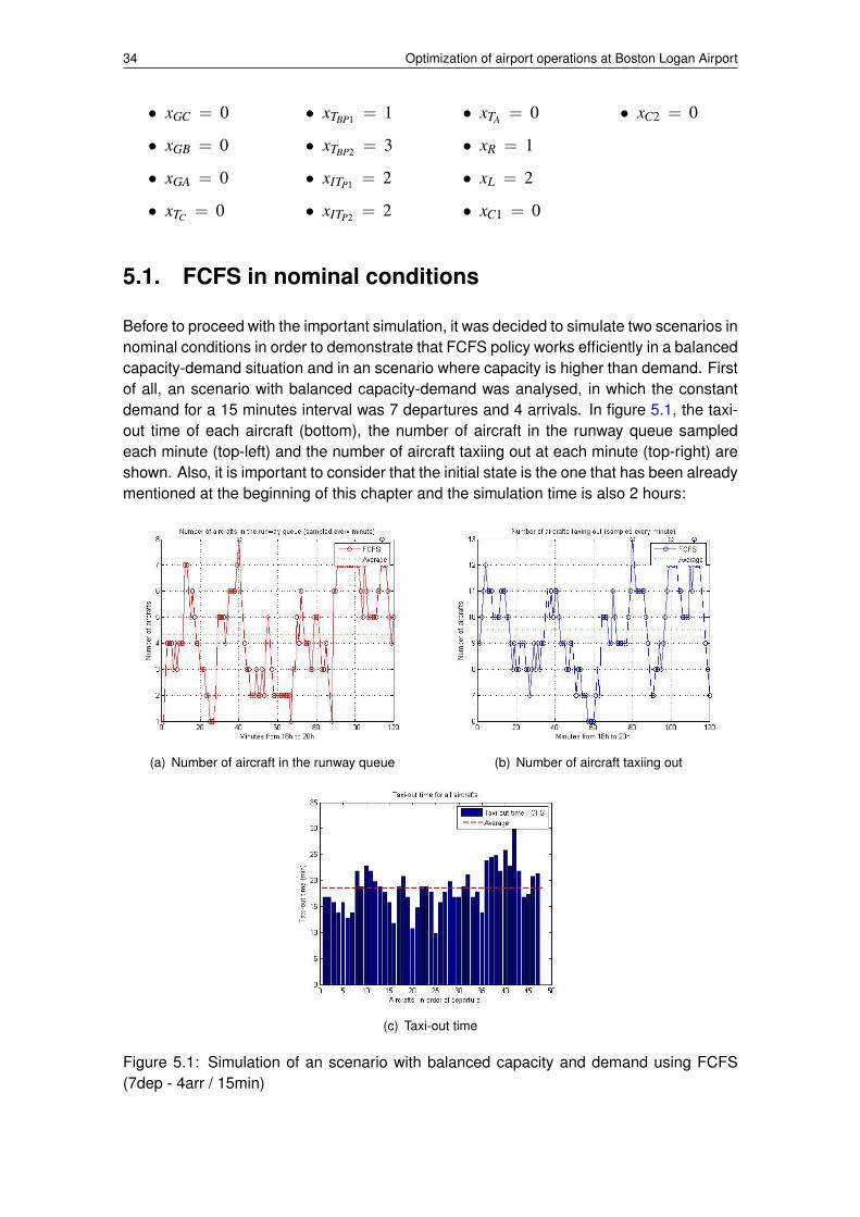
Before to proceed with the important simulation, it was decided to simulate two scenarios innominal conditions in order to demonstrate that FCFS policy works efficiently in a balancedcapacity-demand situation and in an scenario where capacity is higher than demand. Firstof all, an scenario with balanced capacity-demand was analysed, in which the constantdemand for a 15 minutes interval was 7 departures and 4 arrivals. In figure 5.1, the taxi-out time of each aircraft (bottom), the number of aircraft in the runway queue sampledeach minute (top-left) and the number of aircraft taxiing out at each minute (top-right) areshown. Also, it is important to consider that the initial state is the one that has been alreadymentioned at the beginning of this chapter and the simulation time is also 2 hours:
(a) Number of aircraft in the runway queue (b) Number of aircraft taxiing out
(c) Taxi-out time
Figure 5.1: Simulation of an scenario with balanced capacity and demand using FCFS(7dep - 4arr / 15min)

CHAPTER 5. SIMULATION AND RESULTS 35
As we can see, FCFS is able to stabilize the system when it is working in nominal con-ditions of demand, without creating high congestion states. First of all, we can see thatthe average taxi-out time is around 18 minutes, which is close to the unimpeded taxi time,which was determined in section 2.4.1.. The small increment that it suffers in respect tothe unimpeded taxi time is due to the interactions between aircraft on the airport surfaceas well as the different velocities of each aircraft.
Moreover, we can see that the number of aircraft taxiing-out and specifically the number ofaircraft in the runway queue are stable, as they do not increase with the time. The numberof aircraft in the runway queue varies around 4 aircraft during all the test, which meansthat, in this scenario, aircraft will have to do a little bit of queue before departure but nottoo much. This queue is caused for the different distribution of arrivals and departures ineach period of 15 minutes, as we do not know in which of the minutes the external arrivalswill happen. Based on these observations, it can be said, therefore, that there is a balancebetween the external arrivals to the system and the rate in which the aircraft can leave theairport system using FCFS for this scenario.
Secondly, an scenario where capacity is higher than demand was analysed, in which theconstant demand is 7 departures and 3 arrivals. The results are shown in Figure 5.2
(a) Number of aircraft in the runway queue (b) Number of aircraft taxiing out
(c) Taxi-out time
Figure 5.2: Simulation of an scenario with capacity higher than demand using FCFS (7dep- 3arr / 15min)
Of course, in this second scenario the taxi-out time is reduced, as there are less aircraft
36 Optimization of airport operations at Boston Logan Airport
asking for departure and therefore the congestion is even less. In this case, the taxi-outtime is around 14 minutes, which is really close to the unimpeded taxi time, although thereare still some differences due to interactions between aircraft in the surface, as they cannotbe completely eliminated even if there are just a few aircraft taxiing-out at the same time.We can also see that, in this case, there are lots of moments where the number of aircraftin the runway queue is zero, as the current demand is lower than the maximum capacityof the runways and, therefore, they do not have to be used all the time as in the previouscase.
5.2. FCFS and MPC when demand exceeds capacity
Once the good behavior of FCFS in nominal conditions has been proven, it is time to moveto the case in which demand exceeds the capacity, which is the problematic scenario andthe one that requires an improvement. This is basically the objective of this thesis.
In this section, the used scenario is the one described at the beginning of this chapter,with a constant demand of 8 departures and 4 arrivals per 15 minutes period and the initialstate that has been already specified.
In Figure 5.3, the results for this situation by using FCFS are shown, where we can seethe total taxi-out time for all the aircraft (top-left), the taxi-out time for aircraft coming fromterminal C (top-right), the taxi-out time for aircraft coming from terminal B (middle-left),the taxi-out time for aircraft coming from terminal A (middle-right), the number of aircrafttaxiing out (bottom-left) and the number of aircraft which are taxiing out but have alreadyarrived to the runway queue (bottom-right). The reason of showing also the taxi times forthe aircraft coming from each different terminals is to also analyse the fairness betweenairlines by using FCFS or MPC.

CHAPTER 5. SIMULATION AND RESULTS 37
(a) Taxi-out time for each of the aircraft (b) Taxi-out time for aircraft from Terminal C
(c) Taxi-out time for aircraft from Terminal B (d) Taxi-out time for aircraft from Terminal A
(e) Number of aircraft taxiing out at each minute (f) Number of aircraft in the runway queue at eachminute
Figure 5.3: Simulation of an scenario with high demand using FCFS (8dep - 4arr / 15min)
As we can see in Figure 5.3(a), the average taxi-out time in this scenario is around 31minutes, which is a really high value respect to the unimpeded taxi time. This value is dueto the larges queues that take place at the runway threshold, as it is shown in Figure 5.3(f).
Basically, what happens is that the airport cannot meet the departure demand and aircraftstart to accumulate at the runway queue, as FCFS release aircraft from gates once theyare ready for pushback and they taxi until the runway to wait there for the take off. We can

38 Optimization of airport operations at Boston Logan Airport
see that this queue increases with time. The reason is that we have supposed a constantdemand which exceeds the capacity, therefore, each aircraft that cannot take off in itsrespective period because saturation is achieved, remains in the queue. Each 15 minuteperiod there are airplanes which cannot takeoff and, therefore the numbers of aircraft inthe runway queue increases all the time.
Consequently, not only the number of aircraft in the runway queue increases, but also thetaxi-out time, as large delays are absorbed while queuing in the runway. All this extra timein the queue with the engines on, produces a high fuel consumption, which emits a lot ofpolluting emissions to the environment as well as increases the expenses in fuel for theairlines; in fuel that is totally lost just due to an inefficient management.
Also, we can see in Figure 5.3(e) that this instability in the runway queue also occurs in thecount of the aircraft in surface. We have to consider, however, that the number of aircrafton the surface includes the number of aircraft in queue, and hence, this result is totallylogic.
Finally, Figures 5.3(b), 5.3(c) and 5.3(d) shows the taxi-out time but separating the aircraftdepending on the terminal they come from. As it has been already explained in Section4.1., FCFS is a control strategy which is fair with the different airlines, because it releasesaircraft from the gates in the order as they are ready for pushback, which allows them tostart taxiing to the runway and take off in more or less the same order as they were ready.This fairness is also an important factor to analyse, as the objective of this thesis is todevelop a controller that has to be accepted not only for ATC, but also for the airlines.
It is shown in this Figures that there are not aircraft specially injured due to the terminalthey come from. The aircraft that have longer taxi-out times are due to the high queuein the runway, but this effect will have to be faced for aircraft coming from any of theterminals. We can also see that there is a small difference in the average taxi-out time ofthe different terminals; however, this difference is due to the different distance from eachgroup of gates to the runway, as the unimpeded taxi time is already different. Terminal C,which is the closest terminal, has the smallest average taxi-out time and terminal A hasthe biggest, as it is the one that is further.
We just have seen that results obtained for this scenario with FCFS strategy are really bad,as the runway queue is totally unstable and it is reflected in the taxi-out time. Therefore,now a possible solution to this issue by using the proposed method in this thesis is shown.
The dynamics and constraints are the ones that have been explained in section 3. Theexternal arrivals are modeled as explained in Section 4.2.2., with the respective values forthis scenario, which are shown just below.
Rate of pushback from the gates:
AC(k) = 0.1673 acc/minAB(k) = 0.2614 acc/minAA(k) = 0.1046 acc/min
Rate of how the aircraft enter the landing queue:
AL(k) = 0.2667 acc/min
Also, in order to carry out a better analysis, the real external arrivals considered in thefast-time simulation for the MPC will take place at the same minutes than in the FCFS
CHAPTER 5. SIMULATION AND RESULTS 39
simulation. For example, if in the FCFS simulation we had external arrivals to the landingqueue in minutes 34, 55 and 110 from the beginning of the simulation (between others), inthe MPC simulation we will have external arrivals in minutes 34, 55 and 110 too. Therefore,the only differences between the simulations will be the velocities and sizes of the aircraft,which are created in real time following the probability explained in 2.4.1., and the controlvariables.
One last comment about the MPC simulation is that an extra calculation was done in orderto increase the fairness between airlines, as applying only the defined dynamics and theobjective function, the method did not take into account this important factor. This calcula-tion is done at each period of time after the solver has computed the optimal control for thecurrent period and forces the controller to maintain the order in which the aircraft asked thepushback. Basically, it consists in calculating the number of aircraft that should pushbackin that moment (considering the controls of the three groups of gates) and checking whichare the airplanes that have been more time in the gate waiting for the departure. After that,the same number of pushbacks is assigned in the current period, however, it is possiblethat the specific aircraft that are allowed to release change, as fairness has priority. It istrue that these changes can affect the performance of the strategy, because maybe thesolver has predicted to release an aircraft from terminal A (unimpeded taxi time of 15 min-utes), but instead we give the clearance to another one of terminal C (unimpeded time of9 minutes) in order to be fair and, due to that, it arrives to the runway queue when there isstill too much queue. However, even the lose of performance, a calculation to be fair anddo not injure specific aircraft is completely necessary in order to develop a system thatcould be accepted for the airlines.
Furthermore, it should be mentioned that MPC algorithm involves solving a linear programat each period of time, as it was explained in Section 4.2.. The linear program in the caseof study has hundreds of variables and thousand of constraints, but its computation haveto be done in a few seconds. In order to achieve it, it was decided to use Matlab and theoptimization modeling package CVX [17, 18] with the Gurobi solver, which is able to finishthe optimization with less than 3 seconds.
Finally, once all these considerations have been explained, the obtained results for theMPC simulation are shown in Figure 5.4.
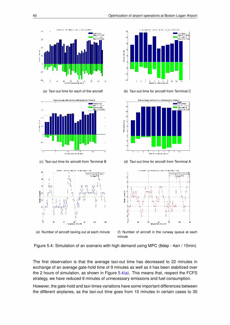
40 Optimization of airport operations at Boston Logan Airport
(a) Taxi-out time for each of the aircraft (b) Taxi-out time for aircraft from Terminal C
(c) Taxi-out time for aircraft from Terminal B (d) Taxi-out time for aircraft from Terminal A
(e) Number of aircraft taxiing out at each minute (f) Number of aircraft in the runway queue at eachminute
Figure 5.4: Simulation of an scenario with high demand using MPC (8dep - 4arr / 15min)
The first observation is that the average taxi-out time has decreased to 22 minutes inexchange of an average gate-hold time of 9 minutes as well as it has been stabilized overthe 2 hours of simulation, as shown in Figure 5.4(a). This means that, respect the FCFSstrategy, we have reduced 9 minutes of unnecessary emissions and fuel consumption.
However, the gate-hold and taxi-times variations have some important differences betweenthe different airplanes, as the taxi-out time goes from 10 minutes in certain cases to 30

CHAPTER 5. SIMULATION AND RESULTS 41
minutes in another ones. This variation, however, does not have special repercussions ata certain terminal, it is produced directly by the special situation that takes place in thesimulation. For example, sometimes the landing aircraft arrive all together at the sametime and consequently the runway queue increases; due to that, aircraft that were alreadytaxiing will start to accumulate at the runway queue and will have to wait until all the aircraftin front of them can take off. This situation can also be the opposite, when there are nolandings and a sequence of departures can take place, decreasing the taxi time for someaircraft. However, that is something that cannot be controlled, as it is caused for theuncertainty of the system.
Gate-holds, on its side, vary from 1 minute to 19 minutes, but just in a few cases, asthe most part of the aircraft wait at the gate for around 10 minutes. We can see that,at the beginning, the gate-holds are really short, due to the low congestion at the firstminutes, but they become longer later on, where the effects of the high demand start tohave consequences.
In Figures 5.4(e) and 5.4(f) we can also see how the MPC control has been able to stabilizethe number of aircraft in the surface and the number of aircraft in the queue. Whereas in theFCFS simulation the runway queue had constantly increased until really undesired stateslike having around 18 aircraft in the runway queue, the MPC strategy has maintained thenumber of aircraft in the runway queue around 6 during all the simulation. Moreover, thenumber of aircraft on the surface has been also stabilized around 11.5 aircraft.
Again, we can see in Figures 5.4(b), 5.3(c) and 5.4(d) that there is not a terminal speciallyaffected. The differences in their average taxi-out time are caused for the same reasonas in the FCFS case: different distances to the runway queue. In this case, however, thedifferences between terminals C, B and A are a little bit higher than in the FCFS case.That is produced because, in the calculation to maintain the order in the pushbacks, it wasconsidered that in case of different aircraft ask for pushback at exactly the same minute,aircraft from terminal C have preference over B and A, and aircraft from terminal B havepreference over terminal A.
Considering only these two simulations, it is clear that we have obtained a far better resultwith the MPC approach. However, the drawbacks of this controller is that its implemen-tation requires a lot of information to be sent to a central computing location at the be-ginning of each period, like the number of aircraft counts in each queue, and the externalarrivals[4].
To help evaluate the performance of MPC versus FCFS, 90 sample simulations (with differ-ent external arrivals distributions for the same demand) were done and its results analysed.In Figure 5.5 the average taxi-out time for each one of the 90 simulations using FCFS andMPC is shown, as well as the total average. Moreover, other important features consid-ering the performance were analysed, like the standard deviation in the average taxi-outtimes, the number of minutes in which the runway queue is empty and the number of sim-ulations in which this undesired effect happens. These characteristics are shown in Table5.2.
In Figure 5.5, we can see that the average taxi-out times for both policies does not differtoo much from their mean in any of the 90 simulations. This fact can also be seen in thecomputed standard deviation shown in Table 5.2, where both deviations are quite small.Specially, we can realize that the approach proposed in this thesis is really reliable, as itsstandard deviation is 0.8664 over 90 simulations. Also, we can also see in the Figure 5.5
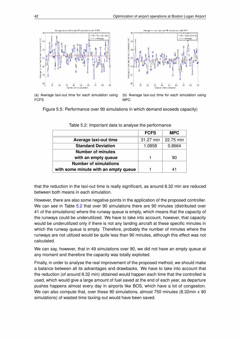
42 Optimization of airport operations at Boston Logan Airport
(a) Average taxi-out time for each simulation usingFCFS
(b) Average taxi-out time for each simulation usingMPC
Figure 5.5: Performance over 90 simulations in which demand exceeds capacity)
Table 5.2: Important data to analyse the performance
FCFS MPC
Average taxi-out time 31.27 min 22.75 minStandard Deviation 1.0858 0.8664Number of minuteswith an empty queue 1 90
Number of simulationswith some minute with an empty queue 1 41
that the reduction in the taxi-out time is really significant, as around 8.32 min are reducedbetween both means in each simulation.
However, there are also some negative points in the application of the proposed controller.We can see in Table 5.2 that over 90 simulations there are 90 minutes (distributed over41 of the simulations) where the runway queue is empty, which means that the capacity ofthe runways could be underutilized. We have to take into account, however, that capacitywould be underutilized only if there is not any landing aircraft at these specific minutes inwhich the runway queue is empty. Therefore, probably the number of minutes where therunways are not utilized would be quite less than 90 minutes, although this effect was notcalculated.
We can say, however, that in 49 simulations over 90, we did not have an empty queue atany moment and therefore the capacity was totally exploited.
Finally, in order to analyse the real improvement of the proposed method, we should makea balance between all its advantages and drawbacks. We have to take into account thatthe reduction (of around 8.32 min) obtained would happen each time that the controlled isused, which would give a large amount of fuel saved at the end of each year, as departurepushes happens almost every day in airports like BOS, which have a lot of congestion.We can also compute that, over these 90 simulations, almost 750 minutes (8.32min x 90simulations) of wasted time taxiing-out would have been saved.
CONCLUSIONS
This thesis presented a decision aiding system for air traffic controllers that helps to im-prove the performance of airport operations, specially to reduce taxi-times and conse-quently unnecessary fuel burn and emissions.
Basically, the underlying dynamics of the developed controller requires the building of anEulerian model to represent the dynamics of the airport of study in a specific runway config-uration. With this model, which is tractable for the purpose of control, different closed-loopcontrol policies can be used. In this thesis, the proposed method was based in MPC, whichallowed to analyze the variation occurred and make good decisions in response to it.
An scenario with an unbalance between capacity and demand was studied and simulationresults using the proposed method (MPC) and the current control strategy in ATC (FCFS)were presented. It was demonstrated that when the maximum throughput of the runwayis not enough to serve all the aircraft that want to take off, the airport can reach high con-gestion states, as aircraft starts to accumulate. However, this congestion can be managedefficiently in order to reduce undesired effects as much as possible.
On one hand, it was shown that, using FCFS, the congestion of the airport was mainlymanifested in the queue of the runway, as all the aircraft were sent there as soon asthey were ready to depart. This management produced long queues at the runway and,consequently, huge taxi-out times of around 31 minutes. On the other hand, it was shownthat MPC was able to reduce the congestion on the surface by keeping the aircraft in thegates. Doing this, the high level of congestion could be distributed over the airport surface,leaving the most part of the aircraft in the gates, where the cost of having aircraft queuesis much less, as they have the engines off and do not waste fuel. In this second case, theaverage taxi-out time was reduced to around 23 minutes, which means that each aircraftsaved around 8 minutes of queue in the runway.
The variability of this control strategies was also analyzed and it was shown that the pro-posed improved strategy is highly reliable, as it has a standard deviation of 0.866 over 90simulations, which is a really small value. Another observation is that the worst taxi-outtime obtained with MPC is 26 minutes, which is still better than any of the results obtainedwith FCFS.
The only point in which FCFS obtains better results than MPC is in exploiting the maximumcapacity of the runway all the time. The MPC produced empty queues in 90 minutes over90 simulations, which in average gives 1 minute per simulation.
Considering all these results, I strongly believe that the proposed method is really usefulin managing high demand situations even with the lost of one minute of runway utilizationeach two hours of simulation. The high reduction in the taxi times is really significant andwe will have lots of savings over the year, which is something that ATC should consider.Moreover, the fact of maintaining the order of the pushbacks as the different aircraft entersthe queue has also been considered, so the proposed method takes also into account thefairness between airlines, which has always been the most remarkable feature of FCFS.
It is true that the information requirements of this controller require to modify a little bitthe underlying dynamics of ATC. However, the new implementation does not require bigchanges, as only systems able to calculate the aircraft count in certain control volumes
43

44 Optimization of airport operations at Boston Logan Airport
are needed, as follow individual aircraft is not necessary to apply this type of control policy.Considering the high benefices of using MPC, the investment for developing systems toobtain the required data could be really worth if we are able to design a real controller thatgives the same benefits than in the simulations.
However, it is important to remark that the proposed method requires minimum levelsof congestion to be really useful, as it was proven that FCFS is efficient in managingsituations with nominal conditions. Therefore, studies should be done to know which is thereal percentage of time in which the application of our controller should be worth.
I would like to comment some future work that could be done to continue testing this con-trol strategy. First of all, the real model should include time-varying restrictions, becausethe throughput of control volumes vary during the day due to different things like weatherconditions. In [4], the introduction of weather forecasts in the model was explained, whichdemonstrates that the proposed Eulerian model is able to include variation in its defini-tion, a part of consider it through the closed-loop nature of the MPC strategy. Also, morecomplicated configurations should be modeled, as well as new challenges included likeconsidering aircraft affected for ground delay programs or any other strategy that is al-ready in use in the airport management.
Finally, I would like to comment that there is still a lot of work to do in order to improvethe performance of airport operations, as demand in air transportation industry is growingevery day and its capacity should increase accordingly. This thesis shows a possibleimprovement to better manage the current capacity, but lots of other options should bealso studied and considered in order to enhance air traffic management, which is essentialfor the possible growth of the aeronautics industry.
BIBLIOGRAPHY
[1] Husni R Idris and R John Hansman. Observation and analysis of departure planningoperations at boston logan international airport. 2011. ix, 4, 5, 8, 10, 11, 12, 14, 18
[2] Ioannis Simaiakis. Modeling and control of airport departure processes for emissionsreduction. PhD thesis, Massachusetts Institute of Technology, 2009. ix, 7, 8
[3] Melanie Sandberg, Tom Reynolds, Harshad Khadilkar, and Hamsa Balakrishnan.Airport characterization for the adaptation of surface congestion management ap-proaches. Technical report, DTIC Document, 2013. ix, 9
[4] Jerome Le Ny and Hamsa Balakrishnan. Feedback control of the national airspacesystem. Journal of Guidance, Control, and Dynamics, 34(3):832–846, 2011. 4, 5, 19,21, 23, 25, 26, 27, 31, 41, 44
[5] Ioannis Simaiakis, Harshad Khadilkar, Hamsa Balakrishnan, Tom G Reynolds, andR John Hansman. Demonstration of reduced airport congestion through pushbackrate control. Transportation Research Part A: Policy and Practice, 66:251–267, 2014.5, 13, 15, 17, 33
[6] Federal Aviation Administration. Aviation system performance metrics (aspm).https://aspm.faa.gov/. Accessed: 2014-01-20. 15
[7] Massport. Logan airport. http://www.massport.com/logan-airport/inside-the-airport/logan-interactive-maps/. Accessed: 2014-01-20. 15,17
[8] http://www.pprune.org/archive/index.php/t-243524.html. Accessed:2015-02-01. 16
[9] Harshad Khadilkar and Hamsa Balakrishnan. Estimation of aircraft taxi fuel burnusing flight data recorder archives. Transportation Research Part D: Transport andEnvironment, 17(7):532–537, 2012. 16
[10] PANS-ATM ICAO. Air traffic management doc. 4444, 2007. 17
[11] Hamsa Balakrishnan. Lecture 10: Terminal Area Operations. 17
[12] Hamsa Balakrishnan. Lecture 12: Surface Operationcs. 17
[13] Issam S Strub and Alexandre M Bayen. Optimal control of air traffic networks usingcontinuous flow models. In AIAA Paper 2006-0228, AIAA Conference on Guidance,Control and Dynamics, 2006. 19
[14] Ronen Perry and Tal Z Zarsky. Queues in law. Iowa L. Rev., 99:1595, 2013. 25
[15] Eduardo F Camacho and Carlos A Bordons. Model predictive control in the processindustry. Springer-Verlag New York, Inc., 1997. 25
[16] Jose Ramon Domınguez Frejo. Control Predictivo cooperativo para el control deredes de trafico mediante el uso de senales ITS. 26
45

[17] Michael Grant, Stephen Boyd, and Yinyu Ye. cvx users’ guide, 2009. 39
[18] Implementing mpc using cvx. Technical report. 39

APPENDICES


APPENDIX A. EXPANDED MATRICES FOR THERESTRICTIONS
In this appendix, the expanded matrix for the restrictions and interactions are shown ex-plicitly.
A.1. Maximum Throughput
The expanded matrices here, as it has been said in Section 3.2.1. correspond to equations3.8 and 3.9 respectively, considering always that they are valid for k ≥ 0 :
1 0 0 0 0 0 0 0 0 0 0 0 0 00 1 0 0 0 0 0 0 0 0 0 0 0 00 0 1 0 0 0 0 0 0 0 0 0 0 00 0 0 0 1 0 0 0 0 0 0 0 0 00 0 0 0 0 1 0 0 0 0 0 0 0 00 0 0 0 0 0 1 0 0 0 0 0 0 00 0 0 0 0 0 0 1 0 0 0 0 0 00 0 0 0 0 0 0 0 1 0 0 0 0 00 0 0 1 0 0 0 0 0 0 0 0 0 00 0 0 0 0 0 0 0 0 1 0 0 0 00 0 0 0 0 0 0 0 0 0 1/2 1/2 0 00 0 0 0 0 0 0 0 0 0 0 0 1 00 0 0 0 0 0 0 0 0 0 0 0 0 1
uCuBuAuABuCI
uBP1uBIuIP1uIRuRuL1uL2uC1uC2
(k)≤
xGC
xGB
xGA
xTC
xTBP1
xTBP2
xITP1
xITP2
xTA
xRxLxC1xC2
(k)+
1 0 0 00 1 0 00 0 1 00 0 0 00 0 0 00 0 0 00 0 0 00 0 0 00 0 0 00 0 0 00 0 0 10 0 0 00 0 0 0
ACABAAAL
(k)
(A.1)
uCuBuAuABuCI
uBP1uBIuIP1uIRuRuL1uL2uC1uC2
(k)≤
22233333311111
(A.2)
A.2. Interactions between Control Volumes
The expanded matrix here, as we said in section 3.2.2. corresponds to equation 3.11:
49
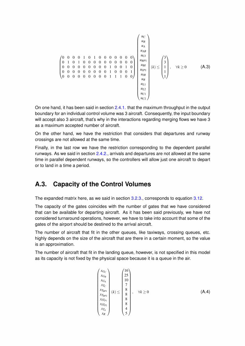
0 0 0 0 1 0 1 0 0 0 0 0 0 00 1 0 1 0 0 0 0 0 0 0 0 0 00 0 0 0 0 0 0 0 0 1 0 0 1 00 0 0 0 0 0 0 0 0 1 0 0 0 10 0 0 0 0 0 0 0 0 1 1 1 0 0
uCuBuAuABuCI
uBP1uBIuIP1uIRuRuL1uL2uC1uC2
(k)≤
33111
, ∀k ≥ 0 (A.3)
On one hand, it has been said in section 2.4.1. that the maximum throughput in the outputboundary for an individual control volume was 3 aircraft. Consequently, the input boundarywill accept also 3 aircraft, that’s why in the interactions regarding merging flows we have 3as a maximum accepted number of aircraft.
On the other hand, we have the restriction that considers that departures and runwaycrossings are not allowed at the same time.
Finally, in the last row we have the restriction corresponding to the dependent parallelrunways. As we said in section 2.4.2., arrivals and departures are not allowed at the sametime in parallel dependent runways, so the controllers will allow just one aircraft to departor to land in a time a period.
A.3. Capacity of the Control Volumes
The expanded matrix here, as we said in section 3.2.3., corresponds to equation 3.12.
The capacity of the gates coincides with the number of gates that we have consideredthat can be available for departing aircraft. As it has been said previously, we have notconsidered turnaround operations, however, we have to take into account that some of thegates of the airport should be destined to the arrival aircraft.
The number of aircraft that fit in the other queues, like taxiways, crossing queues, etc.highly depends on the size of the aircraft that are there in a certain moment, so the valueis an approximation.
The number of aircraft that fit in the landing queue, however, is not specified in this modelas its capacity is not fixed by the physical space because it is a queue in the air.
xGC
xGB
xGA
xTC
xTBP1
xTBP2
xITP1
xITP2
xTA
xR
(k)≤
1625107888845
, ∀k ≥ 0 (A.4)